High order approximations of the log-Heston process semigroup

Abstract.

We present weak approximations schemes of any order for the Heston model that are obtained by using the method developed by Alfonsi and Bally (2021). This method consists in combining approximation schemes calculated on different random grids to increase the order of convergence. We apply this method with either the Ninomiya-Victoir scheme (2008) or a second-order scheme that samples exactly the volatility component, and we show rigorously that we can achieve then any order of convergence. We give numerical illustrations on financial examples that validate the theoretical order of convergence, and present also promising numerical results for the multifactor/rough Heston model.

1. Introduction

The Heston model [16] is one of the most popular model in mathematical finance. It describes the dynamics of an asset and its instantaneous volatility by the following stochastic differential equations:

$$\begin{cases}dS^{s,y}_{t}&=rS^{s,y}_{t}dt+\sqrt{Y^{y}_{t}}S^{s,y}_{t}(\rho dW_{t}+\sqrt{1-\rho^{2}}dB_{t}),\ S^{s,y}_{0}=s>0,\\ dY^{y}_{t}&=(a-bY^{y}_{t})dt+\sigma\sqrt{Y^{y}_{t}}dW_{t},\ Y^{y}_{0}=y\geq 0,\end{cases}$$ (1.1)

where $W$ and $B$ are two independent Brownian motions, $a\geq 0$, $b\in{\mathbb{R}}$, $\sigma>0$ and $\rho\in[-1,1]$. For the financial application, it is typically assumed in addition that $b>0$ so that the volatility mean reverts towards $a/b$, but this is not needed in the present paper.

The goal of the paper is to propose high order weak approximation for this model and to prove their convergence. Let us recall first that exact simulation methods have been proposed for the Heston model by Broadie and Kaya [12] and then by Glasserman and Kim [15]. However, these methods usually require more computation time than simulation schemes. Besides, when considering variants or extensions of the Heston model, it is not clear how to simulate them exactly while approximation schemes can more simply be reused or adapted. There exists in the literature many approximation schemes of the Heston model, we mention here the works of Andersen [9], Lord et al. [17], Ninomiya and Victoir [18] and Alfonsi [2]. Few of them study from a theoretical point of view the weak convergence of these schemes. While [2] focuses on the volatility component, Altmayer and Neuenkirch [8] proposes up to our knowledge the first analysis of the weak error for the whole Heston model. They essentially obtain for a given Euler/Milstein scheme a weak convergence rate of $1$ under the restriction $\sigma^{2}<a$ on the parameter.

Like [8], we will work with the log-Heston model that solves the following SDE

$$\begin{cases}dX^{x,y}_{t}&=(r-\frac{1}{2}Y^{y}_{t})dt+\sqrt{Y^{y}_{t}}(\rho dW_{t}+\sqrt{1-\rho^{2}}dB_{t}),\ X^{x,y}_{0}=x=\log(s)\in{\mathbb{R}},\\ dY^{y}_{t}&=(a-bY^{y}_{t})dt+\sigma\sqrt{Y^{y}_{t}}dW_{t},\ Y^{y}_{0}=y.\end{cases}$$ (1.2)

This log transformation of the asset price is standard to carry mathematical analyses: it allows to get an SDE with bounded moments since its coefficients have at most a linear growth. Our goal is to propose approximations of any order of the semigroup $P_{T}f(x,y)={\mathbb{E}}[f(X^{x,y}_{T},Y^{y}_{T})]$, where $f:{\mathbb{R}}\times{\mathbb{R}}_{+}\to{\mathbb{R}}$ is a sufficiently smooth function such that $|f(x,y)|\leq C(1+|x|^{L}+y^{L})$ for some $L\in{\mathbb{N}}$. More precisely, we want to apply the recent method proposed by Alfonsi and Bally [5] that allows to boost the convergence of an approximation scheme by using random time grids. We consider here either the Ninomiya-Victoir scheme for $\sigma^{2}\leq 4a$ or a scheme that simulate exactly $Y$ for any $\sigma>0$. In a previous work [7], we have applied the method of [5] to the only Cox-Ingersoll-Ross component $Y$ and we want to extend our result to the full log-Heston model. One difficulty with respect to the general framework developed in [5] is to deal with the singularity of the diffusion coefficient. In particular, we need some analytical results on the Cauchy problem associated to the log-Heston model that have been obtained recently by Briani et al. [11]. Our main theoretical result (Theorem 2.1) states that we obtain, for any $\nu\geq 1$, semigroup approximations of order $2\nu$ by using the mentioned scheme with the boosting method of [5].

The paper is structured as follows. Section 2 presents the precise framework and in particular the functional spaces that we consider to carry our analysis. It introduces the approximation schemes and briefly presents the boosting method using random grids proposed in [5]. The main result of the paper is then stated precisely. Section 3 is dedicated to the proof of the main theorem. Last, Section 4 explains how to implement our approximations and illustrates their convergence on numerical experiments motivated by the financial application. As an opening for future research, we show that our approximations can be used for the multifactor Heston model under some parameter restrictions and give very promising convergence results.

2. Main results

We start by introducing some functional spaces that are used through the paper. For $k\in{\mathbb{N}}$, we denote by ${\mathcal{C}}^{k}({\mathbb{R}}\times{\mathbb{R}}_{+})$ the space of continuous functions $f:{\mathbb{R}}\times{\mathbb{R}}_{+}\to{\mathbb{R}}$ such that the partial derivatives $\partial^{\alpha}_{x}\partial^{\beta}_{y}f(x,y)$ exist and are continuous with respect to $(x,y)$ for all $(\alpha,\beta)\in{\mathbb{N}}^{2}$ such that $\alpha+2\beta\leq k$. We then define for $L\in{\mathbb{N}}$,

$${\bf f}_{L}(x,y)=(1+x^{2L}+y^{2L}),\ x\in{\mathbb{R}},y\in{\mathbb{R}}_{+},$$ (2.1)

and introduce

$${\mathcal{C}}^{k,L}_{{\mathbf{pol}}}({\mathbb{R}}\times{\mathbb{R}}_{+})=\{f\in{\mathcal{C}}^{k}({\mathbb{R}}\times{\mathbb{R}}_{+})\mid\exists C>0\text{ such that }\forall(\alpha,\beta)\in{\mathbb{N}}^{2},\alpha+2\beta\leq k,\\ |\partial^{\alpha}_{x}\partial^{\beta}_{y}f(x,y)|\leq C{\bf f}_{L}(x,y)\},$$ (2.2)

the space of continuously differentiable functions up to order $k$ with derivatives with polynomial growth of order $2L$. Note that we assume twice less differentiability on the $y$ component. Furthermore, we set

$${\mathcal{C}}^{k}_{{\mathbf{pol}}}({\mathbb{R}}\times{\mathbb{R}}_{+})=\cup_{L\in{\mathbb{N}}}{\mathcal{C}}^{k,L}_{{\mathbf{pol}}}({\mathbb{R}}\times{\mathbb{R}}_{+})\text{ and }{\mathcal{C}}^{\infty}_{{\mathbf{pol}}}({\mathbb{R}}\times{\mathbb{R}}_{+})=\cap_{k\in{\mathbb{N}}}{\mathcal{C}}^{k}_{{\mathbf{pol}}}({\mathbb{R}}\times{\mathbb{R}}_{+}).$$

Last, we endow ${\mathcal{C}}^{k,L}_{{\mathbf{pol}}}({\mathbb{R}}\times{\mathbb{R}}_{+})$ with the following norm:

$$\|f\|_{k,L}=\sum_{\alpha+2\beta\leq k}\sup_{(x,y)\in{\mathbb{R}}\times{\mathbb{R}}_{+}}\frac{|\partial^{\alpha}_{x}\partial^{\beta}_{y}f(x,y)|}{{\mathbf{f}}_{L}(x,y)}.$$ (2.3)

2.1. Second order schemes for the log-Heston process

Having in mind [3, Theorem 2.3.8], there are three properties to check to get a second-order scheme for the weak error:

1. polynomial estimates for the derivatives of the solution of the Cauchy problem,

2. uniformly bounded moments of the approximation scheme,

3. a potential second order scheme, which roughly means that we have a family of random variables $(\hat{X}^{x,y}_{t},\hat{Y}^{y}_{t})_{t\geq 0}$ such that $|{\mathbb{E}}[f(\hat{X}^{x,y}_{t},\hat{Y}^{y}_{t})]-f(x,y)-t\mathcal{L}f(x,y)-\frac{t^{2}}{2}\mathcal{L}f(x,y)|=_{t\to 0}O(t^{3})$.

Let us precise this in our context. We consider a time horizon $T>0$ and a time step $h=T/n$, with $n\in{\mathbb{N}}^{*}$. We note $(\hat{X}^{x,y}_{h},\hat{Y}^{y}_{h})$ an approximation scheme for the SDE (1.2) starting from $(x,y)$ with time-step $h$, and

$$\hat{P}_{h}f(x,y)={\mathbb{E}}[f(\hat{X}^{x,y}_{h},\hat{Y}^{y}_{h})]$$

the associated semigroup approximation. The weak error analysis proposed by Talay and Tubaro [19] consists in writing

$$\hat{P}^{[n]}_{h}-P_{T}=\hat{P}^{[n]}_{h}-P_{h}^{[n]}=\sum_{i=0}^{n-1}\hat{P}_{h}^{[n-(i+1)]}(\hat{P}_{h}-P_{h})P_{h}^{[i]}=\sum_{i=0}^{n-1}\hat{P}_{h}^{[n-(i+1)]}(\hat{P}_{h}-P_{h})P_{ih},$$ (2.4)

where $\hat{P}_{h}^{[0]}=Id$ and $\hat{P}_{h}^{[i]}=\hat{P}_{h}^{[i-1]}\hat{P}_{h}$ for $i\geq 1$, and $P_{h}^{[i]}=P_{ih}$ by the semigroup property. Let us assume that the three properties hold

1. $\forall k,L\in{\mathbb{N}},\ \exists C\in{\mathbb{R}}_{+},\ \forall i\in\{0,\dots,n\},\ \|P_{ih}f\|_{k,L}\leq C\|f\|_{k,L}$,

2. $\forall L\in{\mathbb{N}},\exists C_{L}\in{\mathbb{R}}_{+},\ \max_{0\leq i\leq n}\hat{P}_{h}^{[i]}{\mathbf{f}}_{L}(x,y)\leq C_{L}{\mathbf{f}}_{L}(x,y)$,

3. $\|\hat{P}_{h}f-P_{h}f\|_{0,L+3}\leq Ch^{3}\|f\|_{12,L}.$

Then, for $f\in{\mathcal{C}}^{12,L}_{{\mathbf{pol}}}({\mathbb{R}}_{+})$, we have for each $i\in\{0,\dots,N-1\},$

$$\|(\hat{P}_{h}-P_{h})P_{ih}f\|_{0,L+3}\leq Ch^{3}\|P_{ih}f\|_{12,L}\leq C^{2}h^{3}\|f\|_{12,L},$$

by using the first and third properties. Then, we use that

$$|(\hat{P}_{h}-P_{h})P_{ih}f(x,y)|\leq C^{2}\|f\|_{12,L}h^{3}{\mathbf{f}}_{L+3}(x,y),$$

together with the second property to get that $|\hat{P}^{[n-(i+1)]}(\hat{P}_{h}-P_{h})P_{ih}f(x,y)|\leq C_{L}C^{2}h^{3}{\mathbf{f}}_{L}(x,y)$. This bound is uniform with respect to $i$, and we get

$$|\hat{P}^{[n]}_{h}f(x,y)-P_{T}f(x,y)|\leq C_{L}C^{2}T{\mathbf{f}}_{L+3}(x,y)\times\left(\frac{T}{n}\right)^{2},$$ (2.5)

since $h=T/n$.

Before concluding this paragraph, we comment briefly how to get the three properties (a–c). For the log-Heston SDE, the Cauchy problem has been studied by Briani et al. [11] and their analysis allow to get (a). Their result is reported in Proposition 3.2. Property (b) can generally be checked by simple but sometimes tedious calculation. Property (c) is the crucial one and can be obtained by using splitting technique, see [3, Paragraph 2.3.2]. We check this property in Corollary 3.7 for the schemes presented in this paper.

2.2. From the second order scheme to higher orders by using random grids

We continue the analysis and present, in our framework, the method developed by Alfonsi and Bally [5] to get approximations of any orders by using random grids. For $\ell\in{\mathbb{N}}^{*}$, let us define the time step $h_{l}=\frac{T}{n^{l}}$. We set $Q_{l}=\hat{P}_{h_{l}}$ the operator obtained by using the approximation scheme with the time step $h_{l}$. The principle is to iterate the identity (2.4). Namely, we get from (2.4)

$$\hat{P}_{h_{1}}^{[i]}-P_{ih_{1}}=\sum_{i_{1}=0}^{i-1}\hat{P}^{[i-(i_{1}+1)]}_{h_{1}}(\hat{P}_{h_{1}}-P_{h_{1}})P^{[i_{1}]}_{h_{1}}$$

and

$$\hat{P}_{h_{2}}^{[n]}-P_{h_{1}}=\hat{P}_{h_{2}}^{[n]}-P_{h_{2}}^{[n]}=\sum_{j=0}^{n-1}\hat{P}^{[n-(j+1)]}_{h_{2}}(\hat{P}_{h_{2}}-P_{h_{2}})P^{[j]}_{h_{2}}.$$

Plugging these two identities successively in (2.4), we obtain

$$\hat{P}^{[n]}_{h_{1}}-P_{T}=\sum_{i=0}^{n-1}\hat{P}_{h_{1}}^{[n-(i+1)]}(\hat{P}_{h_{1}}-\hat{P}_{h_{2}}^{[n]})\hat{P}^{[i]}_{h_{1}}+R,$$ (2.6)

with the remainder given by

$$R= \sum_{i=0}^{n-1}\hat{P}_{h_{1}}^{[n-(i+1)]}\left(\sum_{j=0}^{n-1}\hat{P}^{[n-(j+1)]}_{h_{2}}(\hat{P}_{h_{2}}-P_{h_{2}})P^{[j]}_{h_{2}}\right)\hat{P}^{[i]}_{h_{1}}$$

$$-\sum_{i=0}^{n-1}\hat{P}_{h_{1}}^{[n-(i+1)]}(\hat{P}_{h_{1}}-P_{h_{1}})\sum_{i_{1}=0}^{i-1}\hat{P}^{[i-(i_{1}+1)]}_{h_{1}}(\hat{P}_{h_{1}}-P_{h_{1}})P^{[i_{1}]}_{h_{1}}.$$

Let us assume that we have the two following properties

$$\forall l,k,L\in{\mathbb{N}},\exists C>0,\forall f\in{\mathcal{C}}^{k+12,L}_{{\mathbf{pol}}}({\mathbb{R}}_{+})({\mathbb{R}}\times{\mathbb{R}}_{+}),\,\|(P_{h_{l}}-Q_{l})f\|_{k,L+3}\leq C\|f\|_{k+12,L}h_{l}^{3}, \overline{H_{1}}$$ ()

$$\forall l,k,L\in{\mathbb{N}},\exists C>0,\forall f\in{\mathcal{C}}^{k,L}_{{\mathbf{pol}}}({\mathbb{R}}_{+})({\mathbb{R}}\times{\mathbb{R}}_{+}),\,\max_{0\leq j\leq n^{l}}\|Q^{[j]}_{l}f\|_{k,L}+\sup_{t\leq T}\|P_{t}f\|_{k,L}\leq C\|f\|_{k,L}. \overline{H_{2}}$$ ()

Then, we can upper bound the remainder for $f\in{\mathcal{C}}^{k+24,L}_{{\mathbf{pol}}}({\mathbb{R}}_{+})({\mathbb{R}}\times{\mathbb{R}}_{+})$ by

$$\|Rf\|_{k,L+6}\leq C^{3}n^{2}\|f\|_{k+12,L+3}h_{2}^{3}+C^{5}\frac{n(n-1)}{2}\|f\|_{k+24,L}(h_{1}^{3})^{2}\leq\tilde{C}\|f\|_{k+24,L}\left(\frac{T}{n}\right)^{4},$$

where we have used twice ($\overline{H_{2}}$) and once ($\overline{H_{1}}$) for the first sum, and three times ($\overline{H_{2}}$) and twice ($\overline{H_{1}}$) for the second one. Therefore, we get from (2.6) that

$$\hat{\mathcal{P}}^{2,n}:=\hat{P}^{[n]}_{h_{1}}+\sum_{i=0}^{n-1}\hat{P}_{h_{1}}^{[n-(i+1)]}(\hat{P}_{h_{2}}^{[n]}-\hat{P}_{h_{1}})\hat{P}^{[i]}_{h_{1}}$$ (2.7)

is an approximation of order $4$. Namely, we get

$$\forall f\in{\mathcal{C}}^{24}_{{\mathbf{pol}}}({\mathbb{R}}\times{\mathbb{R}}_{+}),\ \exists C>0,L\in{\mathbb{N}},\ \|\hat{\mathcal{P}}^{2,n}f-P_{T}f\|_{0,L+6}\leq C\|f\|_{24,L}\left(\frac{T}{n}\right)^{4}.$$ (2.8)

Let us note that $\hat{P}_{h_{1}}^{[n-(i+1)]}\hat{P}_{h_{2}}^{[n]}\hat{P}_{h_{1}}^{[i]}$ corresponds to the scheme on a time grid that is uniform, but uniformly refined on the $(i+1)$-th time step. This time grid has thus $2n$ time steps, and if one should calculate all the terms in the sum of (2.7), this would require a computational time in $O(n^{2})$. Thus, the method would not be more efficient that using the second-order scheme with a time step $n^{2}$. This is why we use random grids and use a random variable $\kappa$ that is uniformly distributed on $\{0,\dots,n-1\}$. We have

$$\hat{\mathcal{P}}^{2,n}=\hat{P}^{[n]}_{h_{1}}+n{\mathbb{E}}[\hat{P}_{h_{1}}^{[n-(\kappa+1)]}(\hat{P}_{h_{2}}^{[n]}-\hat{P}_{h_{1}})\hat{P}^{[\kappa]}_{h_{1}}].$$ (2.9)

Thus, for the correcting term, we consider a random time grid that is the obtained from the uniform time grid with time step $T/n$ by refining uniformly the $(\kappa+1)$-th time step with a time step $h_{2}=T/n^{2}$.

We have presented here how $\hat{\mathcal{P}}^{2,n}$ improves the convergence of $\hat{\mathcal{P}}^{1,n}=\hat{P}^{[n]}_{h_{1}}$. Then, for $\nu\geq 2$, it is possible to define by induction approximations $\hat{\mathcal{P}}^{\nu,n}$, such that

$$\forall f\in{\mathcal{C}}^{12\nu}_{{\mathbf{pol}}}({\mathbb{R}}\times{\mathbb{R}}_{+}),\ \exists C>0,L\in{\mathbb{N}},\ \|\hat{\mathcal{P}}^{\nu,n}f-P_{T}f\|_{0,L+3\nu}\leq C\|f\|_{12\nu,L}\left(\frac{T}{n}\right)^{2\nu}.$$ (2.10)

Unfortunately, the induction cannot be easily described and involves a tree structure. We refer to [5] for the details and to [7, Eq. (2.8)] for an explicit expression of $\hat{\mathcal{P}}^{3,n}$.

2.3. A second-order scheme for the log-Heston model

Before presenting the scheme, it is interesting to point similarities and difference between the weak error analysis of Subsection 2.1 and the present one to get higher order approximations. Property ($\overline{H_{1}}$) is a generalization of (c), while ($\overline{H_{2}}$) is stronger than properties (a) and (b). We now point an important difference between the two error analysis. In Equation (2.4), the difference between the semigroup and its approximation appears only once and there is no need to have regularity properties for the function $(\hat{P}_{h}-P_{h})P_{ih}f$: only a polynomial bound is needed. In contrast, for the approximation $\hat{\mathcal{P}}^{2,n}$ we need some regularity to iterate and upper bound the remainder. This difference has an important incidence in the case of the log-Heston process. It is proposed in [2] a second-order scheme for the log-Heston process for any $\sigma\geq 0$. When $\sigma^{2}\geq 4a$, this scheme relies for the Cox-Ingersoll-Ross (CIR) part on bounded random variables that match the first moments of the standard normal distribution. Unfortunately, these moment-matching variables prevent us to get ($\overline{H_{2}}$): in a recent work on high order approximations for the CIR process, we have shown in [7, Theorem 5.16] that it was not possible to use these moment-matching variables together with our analysis in order to get ($\overline{H_{2}}$). We do not repeat here the analysis that would be quite similar for the log-Heston model, and consider either the Ninomiya-Victoir scheme for $\sigma^{2}\leq 4a$ or the exact CIR simulation for any $\sigma>0$. We now present this in detail.

We present in this subsection the approximations scheme that we will study in this paper. It is constructed by using the splitting technique. Let $\overline{\rho}=\sqrt{1-\rho^{2}}$, the infinitesimal generator associated to the log-Heston SDE (1.2) is given by

$${\mathcal{L}}=\frac{y}{2}(\partial^{2}_{x}+2\rho\sigma\partial_{x}\partial_{y}+\sigma^{2}\partial_{y})+(r-\frac{y}{2})\partial_{x}+(a-by)\partial_{y}.$$ (2.11)

We split this operator as the sum ${\mathcal{L}}={\mathcal{L}}_{B}+{\mathcal{L}}_{W}$ where

$${\mathcal{L}}_{B}=\big{(}(r-\frac{\rho a}{\sigma})+(\frac{\rho b}{\sigma}-\frac{1}{2})y\big{)}\partial_{x}+\frac{y}{2}\overline{\rho}^{2}\partial_{x}^{2}$$ (2.12)

is the infinitesimal generator of the SDE

$$\begin{cases}dX_{t}&=\big{(}(r-\frac{\rho a}{\sigma})+(\frac{\rho b}{\sigma}-\frac{1}{2})Y_{t}\big{)}dt+\overline{\rho}\sqrt{Y_{t}}dB_{t},\\ dY_{t}&=0,\end{cases}$$ (2.13)

and

$${\mathcal{L}}_{W}=\frac{y}{2}(\rho^{2}\partial^{2}_{x}+2\rho\sigma\partial_{x}\partial_{y}+\sigma^{2}\partial^{2}_{y})+(a-by)(\frac{\rho}{\sigma}\partial_{x}+\partial_{y})$$ (2.14)

is the infinitesimal generator of

$$\begin{cases}dX_{t}&=(\frac{\rho a}{\sigma}-\frac{\rho b}{\sigma}Y_{t})dt+\rho\sqrt{Y_{t}}dW_{t},\\ dY_{t}&=(a-bY_{t})dt+\sigma\sqrt{Y_{t}}dW_{t}.\end{cases}$$ (2.15)

This splitting is slightly different from the one considered in [2, Subsection 4.2]: one should remark that it is chosen in order to have in (2.15) $dX_{t}=\frac{\rho}{\sigma}dY_{t}$. This is not particularly useful to get a second order scheme. However, it avoids to introduce a third coordinate corresponding to the integrated CIR process, which is more parsimonious for the mathematical analysis.

We now present two different second order schemes for the log-Heston process, for which we will be able to prove the effectiveness of the higher order approximations. The first one simply consists in sampling exactly each SDE and then using the scheme composition introduced by Strang, see e.g. [3, Corollary 2.3.14]. More precisely, let $P^{B}$ (resp. $P^{W}$) denote the semigroup associated to the SDE (2.13) (resp. (2.15)). We define

$$\hat{P}_{t}^{Ex}=P^{B}_{t/2}P^{W}_{t}P^{B}_{t/2}.$$ (2.16)

Let us note that the exact scheme for (2.13) is explicit and given by

$$\varphi_{B}(t,x,y,N)=(x+(r-\rho a/\sigma)t-(1/2-\rho b/\sigma)yt+\overline{\rho}\sqrt{ty}N,~{}y),\ \text{ with }N\sim{\mathcal{N}}(0,1).$$ (2.17)

We indeed have $P^{B}_{t}f(x,y)={\mathbb{E}}[f(\varphi_{B}(t,x,y,N))]$ for all $f\in{\mathcal{C}}^{0}_{{\mathbf{pol}}}({\mathbb{R}}\times{\mathbb{R}}_{+})$. For the SDE (2.15), we have $P^{W}_{t}f(x,y)={\mathbb{E}}[f(x+\frac{\rho}{\sigma}(Y^{y}_{t}-y),Y^{y}_{t})]$, where $Y^{y}$ is the solution of (1.2). Thus, it amounts to simulate exactly the $Y^{y}_{t}$, and we refer to [3, Section 3.1] for a presentation of different exact simulation methods.

However, in practice, the exact simulation of the Cox-Ingersoll-Ross process is longer than a simple Gaussian random variable, and it can be interesting to use an approximation scheme. We use here the one introduced by Ninomiya and Victoir [18]. Following Theorem 1.18 in [2], we rewrite ${\mathcal{L}}_{W}={\mathcal{L}}_{0}+{\mathcal{L}}_{1}$ where

$${\mathcal{L}}_{0}=(a-\frac{\sigma^{2}}{4}-by)(\frac{\rho}{\sigma}\partial_{x}+\partial_{y}),\qquad{\mathcal{L}}_{1}=\frac{y}{2}(\rho^{2}\partial^{2}_{x}+2\rho\sigma\partial_{x}\partial_{y}+\sigma^{2}\partial^{2}_{y})+\frac{\rho\sigma}{4}\partial_{x}+\frac{\sigma^{2}}{4}\partial_{y},$$ (2.18)

are the infinitesimal generator respectively associated to

$$\begin{cases}dX_{t}&=(\frac{\rho}{\sigma}(a-\sigma^{2}/4)-\frac{\rho b}{\sigma}Y_{t})dt\\ dY_{t}&=(a-\sigma^{2}/4-bY_{t})dt\end{cases}\text{ and }\begin{cases}dX_{t}&=\frac{\rho\sigma}{4}dt+\rho\sqrt{Y_{t}}dW_{t}\\ dY_{t}&=\frac{\sigma^{2}}{4}dt+\sigma\sqrt{Y_{t}}dW_{t}.\end{cases}$$

Let $\psi_{b}(t)=\frac{1-e^{-bt}}{b}$ (convention $\psi_{b}(t)=t$ for $b=0$) and define

$$\varphi_{0}(t,x,y) =\Big{(}x-\frac{\rho b}{\sigma}\psi_{b}(t)y+\frac{\rho}{\sigma}\psi_{b}(t)(a-\frac{\sigma^{2}}{4}),~{}e^{-bt}y+\psi_{b}(t)(a-\frac{\sigma^{2}}{4})\Big{)},$$ (2.19)

$$\varphi_{1}(t,x,y) =\Big{(}x+\frac{\rho}{\sigma}\big{(}(\sqrt{y}+\frac{\sigma t}{2})^{2}-y\big{)},~{}(\sqrt{y}+\frac{\sigma t}{2})^{2}\Big{)}.$$ (2.20)

We have for $t\geq 0$ and $f\in{\mathcal{C}}^{0}_{{\mathbf{pol}}}({\mathbb{R}}\times{\mathbb{R}}_{+})$,

$$P^{0}_{t}f(x,y)=f(\varphi_{0}(t,x,y))\text{ and }P^{1}_{t}f(x,y)={\mathbb{E}}[f(\varphi_{1}(\sqrt{t}G,x,y))],\text{ with }G\sim\mathcal{N}(0,1).$$ (2.21)

Indeed, $\varphi_{0}$ is the exact solution of the ODE associated to $\mathcal{L}_{0}$, starting from $(x,y)$ at time $0$, and we can show by Itô calculus that $\varphi_{1}(W_{t},x,y)$ is an exact solution of the SDE associated to $\mathcal{L}_{1}$, starting from $(x,y)$ at time $0$, and with the Brownian motion $d\tilde{W}_{t}=\text{sgn}\left(\sqrt{y}+\frac{\sigma}{2}W_{t}\right)dW_{t}$. The Ninomiya-Victoir scheme [18] for $\mathcal{L}_{W}$ is then $P^{0}_{t/2}P^{1}_{t}P^{0}_{t/2}$, and we define

$$\hat{P}_{t}^{NV}=P^{B}_{t/2}P^{0}_{t/2}P^{1}_{t}P^{0}_{t/2}P^{B}_{t/2},\text{ when }\sigma^{2}\leq 4a.$$ (2.22)

This scheme is well defined only for $\sigma^{2}\leq 4a$, otherwise $\varphi_{0}$ may send the $y$ component to negative values, and the composition is not well defined. This problem was pointed in [2] that introduces a second order scheme for any $\sigma\geq 0$. For this scheme, the normal variable $G$ in (2.21) is replaced by a bounded random variable that matches the five first moments of $G$ and besides, an ad hoc discrete scheme is used in the neighbourhood of $0$. However, as indicated in the introduction of this subsection, this prevents us with our analysis to get ($\overline{H_{2}}$) and thus approximations of higher order. This is why we only consider the Ninomiya-Victoir scheme here.

We now state the main theorem of the paper.

Theorem 2.1.

Let $\hat{P}_{t}$ be either $\hat{P}_{t}^{Ex}$ defined by (2.16) or $\hat{P}_{t}^{NV}$ by (2.22). Let $T>0$, $n\in{\mathbb{N}}^{*}$ and $h_{l}=T/n^{l}$. Let $\hat{\mathcal{P}}^{1,n}=\hat{P}_{h_{1}}^{[n]}$, $\hat{\mathcal{P}}^{2,n}$ be defined by (2.7) and $\hat{\mathcal{P}}^{\nu,n}$ the further approximations developed in [5]. Let $\nu\geq 1$. For any $f\in{\mathcal{C}}^{12\nu}_{{\mathbf{pol}}}({\mathbb{R}}\times{\mathbb{R}}_{+})$ $x\in{\mathbb{R}}$ and $y\geq 0$, we have

$$\hat{\mathcal{P}}^{\nu,n}f(x,y)-P_{T}f(x,y)=O(1/n^{2\nu}).$$

Proof.

Property ($\overline{H_{1}}$) is proved in Corollary 3.7 and ($\overline{H_{2}}$) in Lemma 3.4. For $f\in{\mathcal{C}}^{12\nu}_{{\mathbf{pol}}}({\mathbb{R}}\times{\mathbb{R}}_{+})$, there exists $L$ such that $f\in{\mathcal{C}}^{12\nu,L}_{{\mathbf{pol}}}({\mathbb{R}}\times{\mathbb{R}}_{+})$. Let $\nu=1$. We get from (2.4),

$$\|\hat{\mathcal{P}}^{1,n}f-P_{T}f\|_{0,L}=\|\sum_{i=0}^{n-1}\hat{P}_{h_{1}}^{[n-(i+1)]}(\hat{P}_{h_{1}}-P_{h_{1}})P_{i{h_{1}}}f\|_{0,L}\leq C^{3}T\|f\|_{12,L+3}\left(\frac{T}{n}\right)^{2},$$

since $\|\hat{P}_{h_{1}}^{[n-(i+1)]}(\hat{P}_{h_{1}}-P_{h_{1}})P_{i{h_{1}}}f\|_{0,L}\leq C\|(\hat{P}_{h_{1}}-P_{h_{1}})P_{i{h_{1}}}f\|_{0,L}\leq C^{2}\|P_{i{h_{1}}}f\|_{12,L+3}h_{1}^{3}\leq C^{3}\|f\|_{12,L+3}h_{1}^{3}$ by using ($\overline{H_{2}}$), then ($\overline{H_{1}}$) and again ($\overline{H_{2}}$). This shows the claim for $\nu=1$. For $\nu=2$ (resp. $\nu\geq 3$), the claim is a consequence of (2.8) (resp. (2.10)). ∎

3. Proof of the main result

3.1. Preliminary results on the norm

The next lemma gathers basic properties of the family of norms $\|\cdot\|_{k,L}$ defined in Equation (2.3).

Lemma 3.1.

Let $k,L\in{\mathbb{N}}$. We have the following basic properties:

1. ${\mathcal{C}}^{k+1,L}_{{\mathbf{pol}}}({\mathbb{R}}\times{\mathbb{R}}_{+})\subset{\mathcal{C}}^{k,L}_{{\mathbf{pol}}}({\mathbb{R}}\times{\mathbb{R}}_{+})$. For $f\in{\mathcal{C}}^{k+1,L}_{{\mathbf{pol}}}({\mathbb{R}}\times{\mathbb{R}}_{+})$, we have $\|f\|_{k,L}\leq\|f\|_{k+1,L}$.

2. Let $k,\alpha^{\prime},\beta^{\prime}\in{\mathbb{N}}$. For $f\in{\mathcal{C}}^{k+\alpha^{\prime}+2\beta^{\prime},L}_{{\mathbf{pol}}}({\mathbb{R}}\times{\mathbb{R}}_{+})$ one has $\|\partial_{x}^{\alpha^{\prime}}\partial_{y}^{\beta^{\prime}}f\|_{k,L}\leq\|f\|_{k+\alpha^{\prime}+2\beta^{\prime},L}$.

3. ${\mathcal{C}}^{k,L}_{{\mathbf{pol}}}({\mathbb{R}}\times{\mathbb{R}}_{+})\subset{\mathcal{C}}^{k,L+1}_{{\mathbf{pol}}}({\mathbb{R}}\times{\mathbb{R}}_{+})$ and $\|f\|_{k,L+1}\leq 3\|f\|_{k,L}$ for $f\in{\mathcal{C}}^{k,L}_{{\mathbf{pol}}}({\mathbb{R}}\times{\mathbb{R}}_{+})$.

4. Let ${\mathcal{M}}_{1}$ be the operator defined by ${\mathcal{M}}_{1}f(x,y)=yf(x,y)$. For $f\in{\mathcal{C}}^{k,L}_{{\mathbf{pol}}}({\mathbb{R}}\times{\mathbb{R}}_{+})$, we have ${\mathcal{M}}_{1}f\in{\mathcal{C}}^{k,L+1}_{{\mathbf{pol}}}({\mathbb{R}}\times{\mathbb{R}}_{+})$ and $\|{\mathcal{M}}_{1}f\|_{k,L+1}\leq\frac{3}{2}(k+1)\|f\|_{k,L}$.

5. Let ${\mathcal{L}}$, ${\mathcal{L}}_{B}$, ${\mathcal{L}}_{W}$, ${\mathcal{L}}_{0}$ and ${\mathcal{L}}_{1}$ the infinitesimal generators defined in Equations (2.11), (2.12), (2.14) and (2.18). Then, for all $k\in{\mathbb{N}}$, there exists a constant $C(k)$ such that

   $$\forall L\in{\mathbb{N}},f\in{\mathcal{C}}^{k+4,L}_{{\mathbf{pol}}}({\mathbb{R}}\times{\mathbb{R}}_{+}),\ \|{\mathcal{L}}f\|_{k,L+1}+\|{\mathcal{L}}_{W}f\|_{k,L+1}+\|{\mathcal{L}}_{1}f\|_{k,L+1}\leq C(k)\|f\|_{k+4,L},$$

   $$\forall L\in{\mathbb{N}},f\in{\mathcal{C}}^{k+2,L}_{{\mathbf{pol}}}({\mathbb{R}}\times{\mathbb{R}}_{+}),\ \|{\mathcal{L}}_{B}f\|_{k,L+1}+\|{\mathcal{L}}_{0}f\|_{k,L+1}\leq C(k)\|f\|_{k+2,L}.$$

Proof.

Property (1)-(2) are straightforward. We prove only (3), (4) and (5).

(3) Let $a>0$ than $a^{2L}\leq 1+a^{2L+2}$. So, we get ${\mathbf{f}}_{L}(x,y)=1+x^{2L}+y^{2L}\leq 3(1+x^{2(L+1)}+y^{2(L+1)})=3{\mathbf{f}}_{L+1}(x,y)$ and then $\frac{1}{{\mathbf{f}}_{L+1}(x,y)}\leq 3\frac{1}{{\mathbf{f}}_{L}(x,y)}$. This gives immediately the claim.

(4) Let $f\in{\mathcal{C}}^{k,L}_{{\mathbf{pol}}}({\mathbb{R}}\times{\mathbb{R}}_{+})$. Applying Leibniz rule, one obtains $\partial^{\alpha}_{x}\partial_{y}^{\beta}{\mathcal{M}}_{1}f=\beta\partial^{\alpha}_{x}\partial_{y}^{\beta-1}f+{\mathcal{M}}_{1}\partial^{\alpha}_{x}\partial_{y}^{\beta}f$ for $\alpha,\beta\in{\mathbb{N}}$. Now, we write

$$\frac{|\partial^{\alpha}_{x}\partial_{y}^{\beta}[yf(x,y)]|}{{\mathbf{f}}_{L+1}(x,y)} \leq\frac{\beta|\partial^{\alpha}_{x}\partial_{y}^{\beta-1}f(x,y)|}{{\mathbf{f}}_{L+1}(x,y)}+\frac{y|\partial^{\alpha}_{x}\partial_{y}^{\beta}f(x,y)|}{{\mathbf{f}}_{L+1}(x,y)}$$

$$\leq\frac{3\beta|\partial^{\alpha}_{x}\partial_{y}^{\beta-1}f(x,y)|}{{\mathbf{f}}_{L}(x,y)}+\frac{3|\partial^{\alpha}_{x}\partial_{y}^{\beta}f(x,y)|}{2{\mathbf{f}}_{L}(x,y)},$$

where we used the comparison above between ${\mathbf{f}}_{L}$ and ${\mathbf{f}}_{L+1}$ for the first term and, for the second term, $y{\mathbf{f}}_{L}(x,y)=y+y^{2L+1}+yx^{2L}+\leq 1+y^{2L+2}+\frac{1+y^{2}}{2}x^{2L}\leq\frac{3}{2}{\mathbf{f}}_{L+1}(x,y)$ by using $y+y^{2L+1}\leq 1+y^{2L+2}$ and then Young’s inequality. Then, we obtain

$$\|{\mathcal{M}}_{1}f\|_{k,L+1} \leq\sum_{\alpha+2\beta\leq k}\left(3\beta\sup_{(x,y)\in{\mathbb{R}}\times{\mathbb{R}}_{+}}\frac{3\beta|\partial^{\alpha}_{x}\partial_{y}^{\beta-1}f(x,y)|}{{\mathbf{f}}_{L}(x,y)}+\frac{3}{2}\sup_{(x,y)\in{\mathbb{R}}\times{\mathbb{R}}_{+}}\frac{3\beta|\partial^{\alpha}_{x}\partial_{y}^{\beta}f(x,y)|}{{\mathbf{f}}_{L}(x,y)}\right)$$

$$\leq 3\left(\lfloor k/2\rfloor+1/2\right)\|f\|_{k,L}.$$

(5) We prove only the estimate for ${\mathcal{L}}$, the others are obtained using the same arguments. We have $\|{\mathcal{L}}f\|_{k,L+1}\leq\frac{1}{2}\|{\mathcal{M}}_{1}(\partial_{x}^{2}+2\rho\sigma\partial_{x}\partial_{y}+\sigma^{2}\partial_{y}^{2}-\partial_{x}-2b\partial_{y})f\|_{k,L+1}+\|(r\partial_{x}+a\partial_{y})f\|_{k,L+1}$, by using linearity of derivatives and the triangular inequality. We conclude using property (4) and (2) for the first term, (2) and (3) for the second and finally property number (1) to upper bound $\|{\mathcal{L}}f\|_{k,L+1}$ by $C(k)\|f\|_{k+4,L+1}$, where $C(k)$ is a constant depending on $k$ and on the parameters ($r,\rho,a,b$ and $\sigma$). ∎

3.2. The Cauchy problem of the Log-Heston SDE

In this subsection, we aim at proving the estimates on the derivatives of the Cauchy problem. The representation formula presented below is a result of Briani, Caramellino and Terenzi [11].

Proposition 3.2.

Let $k,L\in\mathbb{N}$ and suppose that $f\in{\mathcal{C}}^{k,L}_{{\mathbf{pol}}}({\mathbb{R}}\times{\mathbb{R}}_{+})$. Let $\lambda\geq 0$, $c,d\in{\mathbb{R}}$. Let $(X^{t,x,y},Y^{t,y})$ be the solution to the SDE, for $s\geq t$,

$$\begin{cases}X^{t,x,y}_{s}&=x+\int_{t}^{s}(c+dY^{y}_{r})dr+\int_{t}^{s}\lambda\sqrt{Y^{y}_{r}}(\rho dW_{r}+\sqrt{1-\rho^{2}}dB_{r})\\ Y^{t,y}_{s}&=y+\int_{t}^{s}(a-bY^{y}_{r})dr+\sigma\int_{t}^{s}\sqrt{Y^{y}_{r}}dW_{r}.\end{cases}$$ (3.1)

and set

$$u(t,x,y)={\mathbb{E}}[f(X_{T}^{t,x,y},Y_{T}^{t,y})]=P_{T-t}f(x,y).$$

Then, $u(t,\cdot,\cdot)\in{\mathcal{C}}^{k,L}_{{\mathbf{pol}}}({\mathbb{R}}\times{\mathbb{R}}_{+})$ and the following stochastic representation holds for $\alpha+2\beta\leq k$,

$$\partial_{x}^{\alpha}\partial_{y}^{\beta}u(t,x,y)={\mathbb{E}}\bigg{[}e^{-\beta b(T-t)}\partial_{x}^{\alpha}\partial_{y}^{\beta}f\big{(}X_{T}^{\beta,t,x,y},Y_{T}^{\beta,t,y}\big{)}\\ \quad+\beta\int_{t}^{T}e^{-\beta b(s-t)}\Big{(}\frac{\lambda^{2}}{2}\partial_{x}^{\alpha+2}\partial_{y}^{\beta-1}u+d\partial_{x}^{\alpha+1}\partial_{y}^{\beta-1}u\Big{)}\big{(}s,X_{s}^{\beta,t,x,y},Y_{s}^{\beta,t,y}\big{)}ds\bigg{]},$$ (3.2)

where $\partial_{x}^{\alpha}\partial_{y}^{\beta-1}u:=0$ when $\beta=0$ and $(X^{\beta,t,x,y},Y^{\beta,t,y}),\beta\geq 0$, denotes the solution starting from $(x,y)$ at time $t$ to the SDE (3.1) with parameters

$$\rho_{\beta}=\rho,\quad a_{\beta}=a+\beta\frac{\sigma^{2}}{2},\quad b_{\beta}=b,\quad c_{\beta}=r+\beta\rho\sigma\lambda,\quad d_{\beta}=d,\quad\sigma_{\beta}=\sigma.$$ (3.3)

Moreover, one has the following norm estimation for the semigroup

$$\forall k,L\in{\mathbb{N}},T>0,\ \exists C,\forall f\in{\mathcal{C}}^{k,L}_{{\mathbf{pol}}}({\mathbb{R}}\times{\mathbb{R}}_{+}),t\in[0,T],\ \|P_{t}f\|_{k,L}\leq\|f\|_{k,L}e^{Ct}.$$ (3.4)

Proof.

Proposition 3.2 basically restates [11, Proposition 5.3] in our framework (note that our space ${\mathcal{C}}^{k,L}_{{\mathbf{pol}}}({\mathbb{R}}\times{\mathbb{R}}_{+})$ already includes twice more derivatives in $x$ than in $y$ and that we have added the scaling factor $\lambda$ for convenience). The only additional result is the norm estimate, which we prove now.

Let $f\in{\mathcal{C}}^{k,L}_{{\mathbf{pol}}}({\mathbb{R}}\times{\mathbb{R}}_{+})$. We will prove that for all $(\alpha,\beta)$ such that $\alpha+2\beta\leq k$, there exists a constant $C\in{\mathbb{R}}_{+}$ such that

$$\sup_{x\in{\mathbb{R}}y\in{\mathbb{R}}_{+}}\frac{|\partial_{x}^{\alpha}\partial_{y}^{\beta}u(t,x,y)|}{{\mathbf{f}}_{L}(x,y)}\leq\sup_{x\in{\mathbb{R}}y\in{\mathbb{R}}_{+}}\frac{|\partial_{x}^{\alpha}\partial_{y}^{\beta}f(x,y)|}{{\mathbf{f}}_{L}(x,y)}e^{C(T-t)}+C\|f\|_{k,L}(T-t).$$ (3.5)

Let us note that this implies $\sup_{x\in{\mathbb{R}}y\in{\mathbb{R}}_{+}}\frac{|\partial_{x}^{\alpha}\partial_{y}^{\beta}u(t,x,y)|}{{\mathbf{f}}_{L}(x,y)}\leq\tilde{C}\|f\|_{k,L}$, with $\tilde{C}=e^{CT}+CT$.

For $\beta=0$, the estimate is straightforward : from (3.2) and $f\in{\mathcal{C}}^{k,L}_{{\mathbf{pol}}}({\mathbb{R}}\times{\mathbb{R}}_{+})$, one has

$$|\partial_{x}^{\alpha}u(t,x,y)|\leq\left(\sup_{x^{\prime}\in{\mathbb{R}}y^{\prime}\in{\mathbb{R}}_{+}}\frac{|\partial_{x}^{\alpha}f(x^{\prime},y^{\prime})|}{{\mathbf{f}}_{L}(x^{\prime},y^{\prime})}\right){\mathbb{E}}\big{[}{\mathbf{f}}_{L}(X^{t,x,y}_{T},Y_{T}^{t,y})\big{]},$$

and we get easily (3.5) by using the estimate on moments (3.6) that we prove below.

Suppose now that the estimate (3.5) is true up to $\beta-1$, and let us prove it for $\beta$. Using (3.2) and the induction hypothesis for the integral term, we get

$$|\partial_{x}^{\alpha}\partial_{y}^{\beta}u(t,x,y)|\leq e^{-\beta b(T-t)}\left(\sup_{x^{\prime}\in{\mathbb{R}}y^{\prime}\in{\mathbb{R}}_{+}}\frac{|\partial_{x}^{\alpha}\partial_{y}^{\beta}f(x^{\prime},y^{\prime})|}{{\mathbf{f}}_{L}(x^{\prime},y^{\prime})}\right){\mathbb{E}}\left[{\mathbf{f}}_{L}(X^{\beta,t,x,y}_{T},Y^{\beta,t,y}_{T})\right]$$

$$+\beta\frac{\lambda^{2}+|d|}{2}e^{\beta|b|T}\tilde{C}\|f\|_{k,L}\int_{t}^{T}{\mathbb{E}}[{\mathbf{f}}_{L}(X^{\beta,t,x,y}_{s},Y^{\beta,t,y}_{s})]ds.$$

This gives (3.5) by using again the estimate on the moments (3.6). This shows (3.5) by induction, and we finally sum (3.5) over $\alpha+2\beta\leq k$ to get

$$\|P_{T-t}f\|_{k,L}\leq\|f\|_{k,L}e^{C(T-t)}+C(k+1)^{2}\|f\|_{k,L}(T-t)\leq\|f\|_{k,L}e^{C(1+(k+1)^{2})(T-t)},$$

proving the claim. ∎

Lemma 3.3.

Let $(X^{x,y},Y^{y})$ be the solution of (3.1) starting from $(x,y)$ at time $0$. Let $T>0$. For any $L\in{\mathbb{N}}$, there is a constant $C\in{\mathbb{R}}_{+}$ depending on $T$, $L$ and the SDE parameters, such that

$${\mathbb{E}}[{\mathbf{f}}_{L}(X^{x,y}_{t},Y^{y}_{t})]\leq e^{Ct}{\mathbf{f}}_{L}(x,y),\ t\in[0,T].$$ (3.6)

Proof.

We use the affine (and thus polynomial) property of the extended log-Heston process (3.1), see [13, Example 3.1]. By [13, Theorem 2.7], we get that the log-Heston semigroup acts as a matrix exponential on the polynomial functions of degree lower than $2L$. This gives ${\mathbb{E}}[(X^{x,y}_{t})^{2L}+(Y^{y}_{t})^{2L}]=x^{2L}+y^{2L}+\sum_{i+j\leq 2L}\varphi_{i,j}(t)x^{i}y^{j}$, with $\varphi_{i,j}\in\mathcal{C}^{1}([0,T],{\mathbb{R}})$ such that $\varphi_{i,j}(0)=0$. Using that $|x|^{i}y^{j}\leq|x|^{i+j}+y^{i+j}\leq 2{\mathbf{f}}_{L}(x,y)$ for $i+j\leq 2L$ and using that $\varphi^{\prime}_{i,j}$ is bounded on $[0,T]$, we get

$${\mathbb{E}}[{\mathbf{f}}_{L}(X^{x,y}_{t},Y^{y}_{t})]\leq{\mathbf{f}}_{L}(x,y)+Ct{\mathbf{f}}_{L}(x,y)\leq{\mathbf{f}}_{L}(x,y)e^{Ct},$$

with $C=2\sum_{i,j\leq 2L}\max_{[0,T]}|\varphi^{\prime}_{i,j}|$. ∎

3.3. Proof of ($\overline{H_{1}}$) and  ($\overline{H_{2}}$)

We start by proving the property ($\overline{H_{2}}$) in the next lemma.

Lemma 3.4.

Let $t\in[0,T]$, $k,L\in{\mathbb{N}}$ and $f\in{\mathcal{C}}^{k,L}_{{\mathbf{pol}}}({\mathbb{R}}\times{\mathbb{R}}_{+})$. Let $\varphi_{0}$ be the function defined in Equation (2.19). Then, there exists $C$ such that, for $I\in\{0,1,B,W\}$, $\|P^{I}_{t}f\|_{k,L}\leq e^{Ct}\|f\|_{k,L}$, for $t\in[0,T]$. The semigroup approximations $\hat{P}^{Ex}_{t}$ and $\hat{P}^{NV}_{t}$ enjoy the same property and satisfy ($\overline{H_{2}}$).

Proof.

We apply four times Proposition 3.2 with

• $\tilde{a}=a-\frac{\sigma^{2}}{4}$, $\tilde{b}=b$, $\tilde{c}=\frac{\rho}{\sigma}\left(a-\frac{\sigma^{2}}{4}\right)$, $\tilde{d}=-b\frac{\rho}{\sigma}$, $\tilde{\lambda}=0$, $\tilde{\sigma}=0$ for $P^{0}$,

• $\tilde{a}=\frac{\sigma^{2}}{4}$, $\tilde{b}=0$, $\tilde{c}=\frac{\rho\sigma}{4}$, $\tilde{d}=0$, $\tilde{\lambda}=\rho$, $\tilde{\sigma}=\sigma$, $\tilde{\rho}=1$ for $P^{1}$,

• $\tilde{a}=0$, $\tilde{b}=0$, $\tilde{c}=r-\frac{\rho a}{\sigma}$, $\tilde{d}=\frac{\rho b}{\sigma}-\frac{1}{2}$, $\tilde{\lambda}=\bar{\rho}$, $\tilde{\sigma}=0$, $\tilde{\rho}=0$ for $P^{B}$,

• $\tilde{a}=a$, $\tilde{b}=b$, $\tilde{c}=\frac{\rho a}{\sigma}$, $\tilde{d}=-\frac{\rho b}{\sigma}$, $\tilde{\lambda}=\rho$, $\tilde{\sigma}=\sigma$, $\tilde{\rho}=1$ for $P^{W}$,

where the tilde parameters are the ones used in Equation (3.1). This gives the first claim. Then, we deduce easily that $\|\hat{P}^{Ex}_{t}f\|_{k,L}\leq e^{Ct/2}\|P^{W}_{t}P^{B}_{t/2}f\|_{k,L}\leq e^{2Ct}\|f\|_{k,L}$ by using twice the estimate for $P^{B}$ and once for $P^{W}$. Similarly, we obtain $\|\hat{P}_{t}f\|_{k,L}\leq e^{3Ct}\|f\|_{k,L}$, by using the estimates for $P^{B}$, $P^{0}$ and $P^{1}$.

Now, the property ($\overline{H_{2}}$) follows easily: consider $l\geq 1$ and $Q_{l}=\hat{P}^{NV}_{\frac{T}{n^{l}}}$, we have for $f\in{\mathcal{C}}^{k,L}_{{\mathbf{pol}}}({\mathbb{R}}\times{\mathbb{R}}_{+})$, $\|Q_{l}f\|_{k,L}\leq e^{3C\frac{T}{n^{l}}}$ and thus for any $j\leq n^{l}$, $\|Q^{[j]}_{l}f\|_{k,L}\leq e^{3C\frac{jT}{n^{l}}}\leq e^{3CT}$, which gives ($\overline{H_{2}}$). The same result holds for $\hat{P}^{Ex}$. ∎

We now turn to the proof of the property ($\overline{H_{1}}$). We first state a general result on the composition of approximation schemes that fits our framework with the norm family $\|\cdot\|_{k,L}$. It can be seen as a variant of [3, Proposition 2.3.12] and says, heuristically, that the composition of schemes works as a composition of operators.

Lemma 3.5.

(Scheme composition). Let $\nu\in{\mathbb{N}}$ and $T>0$. Let $V_{i}$, $i\in\{1,\dots,I\}$, be infinitesimal generators such that there exists $k_{i},L_{i}\in{\mathbb{N}}$ such that

$$\forall k\in{\mathbb{N}},\exists C\in{\mathbb{R}}_{+},\forall f\in{\mathcal{C}}^{k+k_{i},L}_{{\mathbf{pol}}}({\mathbb{R}}\times{\mathbb{R}}_{+}),V_{i}f\in{\mathcal{C}}^{k,L+L_{i}}_{{\mathbf{pol}}}({\mathbb{R}}\times{\mathbb{R}}_{+})\text{ and }\|V_{i}f\|_{k,L+L_{i}}\leq C\|f\|_{k+k_{i},L}.$$ (3.7)

Let $k^{\star}=\max_{1\leq i\leq I}k_{i}$ and $L^{\star}=\max_{1\leq i\leq I}L_{i}$. We assume that for any $i$, $\hat{P}^{i}_{t}:{\mathcal{C}}^{0,L}_{{\mathbf{pol}}}({\mathbb{R}}\times{\mathbb{R}}_{+})\to{\mathcal{C}}^{0,L}_{{\mathbf{pol}}}({\mathbb{R}}\times{\mathbb{R}}_{+})$ is such that

$$\forall k,L\in{\mathbb{N}},0\leq\bar{q}\leq\nu+1, \ \exists C,\ \forall f\in{\mathcal{C}}^{k+\bar{q}k_{i},L}_{{\mathbf{pol}}}({\mathbb{R}}\times{\mathbb{R}}_{+}),\forall t\in[0,T],$$

$$\|\hat{P}^{i}_{t}f-\sum_{q=0}^{\bar{q}-1}\frac{t^{q}}{q!}V_{i}^{q}f\|_{k,L+\bar{q}L_{i}}\leq Ct^{\bar{q}}\|f\|_{k+\bar{q}k_{i},L}.$$ (3.8)

Then, we have for $\lambda_{1},\dots,\lambda_{I}\in[0,1]$,

$$\forall k,L\in{\mathbb{N}},0\leq\bar{q}\leq\nu+1,\ \exists C,\forall f\in{\mathcal{C}}^{k+\bar{q}k^{\star},L}_{{\mathbf{pol}}}({\mathbb{R}}\times{\mathbb{R}}_{+}),\forall t\in[0,T]$$

$$\left\|\hat{P}^{I}_{\lambda_{I}t}\dots\hat{P}^{1}_{\lambda_{1}t}f-\sum_{q_{1}+\dots+q_{I}\leq\bar{q}-1}\frac{\lambda_{1}^{q_{1}}\dots\lambda_{I}^{q_{I}}t^{q_{1}+\dots+q_{I}}}{q_{1}!\dots q_{I}!}V_{I}^{q_{I}}\dots V_{1}^{q_{1}}f\right\|_{k,L+\bar{q}L^{\star}}\leq Ct^{\bar{q}}\|f\|_{k+\bar{q}k^{\star},L}.$$ (3.9)

Proof.

For readability, we make the proof with $I=2$ operators. Let $\bar{q}\leq\nu+1$ and $f\in{\mathcal{C}}^{k+\bar{q}k^{\star},L}_{{\mathbf{pol}}}({\mathbb{R}}\times{\mathbb{R}}_{+})$. We define $R^{1}f=\hat{P}^{1}_{\lambda_{1}t}f-\sum_{q_{1}=0}^{\bar{q}-1}\frac{\lambda_{1}^{q_{1}}t^{q_{1}}}{q_{1}!}V_{1}^{q_{1}}f$. For $t\in[0,T]$, we have $\lambda_{1}t\in[0,T]$ since $\lambda_{1}\in[0,1]$ and by assumption (3.8), we have $R^{1}f\in{\mathcal{C}}^{k+\bar{q}k^{\star}-\bar{q}k_{1},L+\bar{q}L_{1}}_{{\mathbf{pol}}}({\mathbb{R}}\times{\mathbb{R}}_{+})$ and

$$\|R^{1}f\|_{k+\bar{q}k^{\star}-\bar{q}k_{1},L+\bar{q}L_{1}}\leq Ct^{\bar{q}}\|f\|_{k+\bar{q}k^{\star},L}.$$

We now write

$$\hat{P}^{2}_{\lambda_{2}t}\hat{P}^{1}_{\lambda_{1}t}f=\sum_{q_{1}=0}^{\bar{q}-1}\frac{\lambda_{1}^{q_{1}}t^{q_{1}}}{q_{1}!}\hat{P}^{2}_{\lambda_{2}t}V_{1}^{q_{1}}f+\hat{P}^{2}_{\lambda_{2}t}R^{1}f.$$

Since $V_{1}^{q_{1}}f\in{\mathcal{C}}^{k+\bar{q}k^{\star}-q_{1}k_{1},L+q_{1}L_{1}}_{{\mathbf{pol}}}({\mathbb{R}}\times{\mathbb{R}}_{+})$, we apply (3.8) to get

$$\hat{P}^{2}_{\lambda_{2}t}V_{1}^{q_{1}}f=\sum_{q_{2}=0}^{\bar{q}-q_{1}-1}\frac{\lambda_{2}^{q_{2}}t^{q_{2}}}{q_{2}!}V_{2}^{q_{2}}V_{1}^{q_{1}}f+R^{2}_{q_{1}}f,$$

with $\|R^{2}_{q_{1}}f\|_{k+\bar{q}k^{\star}-q_{1}k_{1}-(\bar{q}-q_{1})k_{2},L+q_{1}L_{1}+(\bar{q}-q_{1})L_{2}}\leq Ct^{\bar{q}-q_{1}}\|f\|_{k+\bar{q}k^{\star},L}$ by (3.7) and (3.8). We also have $\|\hat{P}^{2}_{\lambda_{2}t}R^{1}f\|_{k+\bar{q}k^{\star}-\bar{q}k_{1},L+\bar{q}L_{1}}\leq Ct^{\bar{q}}\|f\|_{k+\bar{q}k^{\star},L}$ by (3.8). Since

$$k+\bar{q}k^{\star}-q_{1}k_{1}-(\bar{q}-q_{1})k_{2}\geq k,\ L+q_{1}L_{1}+(\bar{q}-q_{1})L_{2}\leq L+\bar{q}L^{\star},$$

for all $0\leq q_{1}\leq\bar{q}-1$, and using Lemma 3.1 (1 and 3), we get

$$\left\|\hat{P}^{2}_{\lambda_{2}t}\hat{P}^{1}_{\lambda_{1}t}f-\sum_{q_{1}+q_{2}\leq\bar{q}-1}\lambda_{1}^{q_{1}}\lambda_{2}^{q_{2}}\frac{t^{q_{1}}t^{q_{2}}}{q_{1}!q_{2}!}V_{2}^{q_{2}}V_{1}^{q_{1}}f\right\|_{k,L+\bar{q}L^{\star}}\leq Ct^{\bar{q}}\|f\|_{k+\bar{q}k^{\star},L}.\qed$$

Lemma 3.6.

Let $L_{0}=L_{1}=L_{B}=L_{W}=L_{H}=1$, $k_{0}=k_{B}=2$, $k_{1}=k_{W}=k_{H}=4$. Let denote ${\mathcal{L}}_{H}={\mathcal{L}}$ and $P^{H}_{t}=P_{t}$ the log-Heston semigroup. Let $i\in\{0,1,B,W,H\}$. We have

$$\forall k,L\in{\mathbb{N}},\exists C\in{\mathbb{R}}_{+},\forall f\in{\mathcal{C}}^{k+k_{i},L}_{{\mathbf{pol}}}({\mathbb{R}}\times{\mathbb{R}}_{+}),\ \|\mathcal{L}_{i}f\|_{k,L+L_{i}}\leq C\|f\|_{k+k_{i},L}.$$

Besides, for any $\bar{q}\in{\mathbb{N}}$, we have

$$\forall k,L\in{\mathbb{N}},\ \exists C,\ \forall f\in{\mathcal{C}}^{k+\bar{q}k_{i},L}_{{\mathbf{pol}}}({\mathbb{R}}\times{\mathbb{R}}_{+}),\|P^{i}_{t}f-\sum_{q=0}^{\bar{q}-1}\frac{t^{q}}{q!}\mathcal{L}_{i}^{q}f\|_{k,L+\bar{q}L_{i}}\leq Ct^{\bar{q}}\|f\|_{k+\bar{q}k_{i},L}.$$

Proof.

The first part of the statement is proved in Lemma 3.1. For $\bar{q}=0$, the estimate is simply the one given by Lemma 3.4 (or Proposition 3.2 for $P^{H}_{t}$).

We now consider $\bar{q}\geq 1$. As already pointed in the proof of Lemma 3.4, each operator is the infinitesimal generator of (3.1) with a suitable choice of parameter. Then, by applying Itô’s formula and taking the expectation, we get $P^{i}_{t}f(x,y)=f(x,y)+\int_{0}^{t}P^{i}_{s}\mathcal{L}_{i}f(x,y)ds$. By iterating, we obtain for $f\in{\mathcal{C}}^{k+\bar{q}k_{i},L}_{{\mathbf{pol}}}({\mathbb{R}}\times{\mathbb{R}}_{+})$,

$$P^{i}_{t}f(x,y)=\sum_{j=0}^{\bar{q}-1}\frac{t^{j}}{j!}{\mathcal{L}}_{i}^{j}f(x,y)+\int_{0}^{t}\frac{(t-s)^{\bar{q}-1}}{(\bar{q}-1)!}P^{i}_{s}{\mathcal{L}}^{\bar{q}}_{i}f(x,y)ds.$$ (3.10)

We have $\|{\mathcal{L}}^{\bar{q}}_{i}f\|_{k,L+\bar{q}L_{i}}\leq C^{\bar{q}}\|f\|_{k+\bar{q}k_{i},L}$ by Lemma 3.1-(5) and thus $\|P^{i}_{s}{\mathcal{L}}^{\bar{q}}_{i}f\|_{k,L+\bar{q}L_{i}}\leq C^{q+1}\|f\|_{k+\bar{q}k_{i},L}$ for $s\in[0,T]$, by using the result for $\bar{q}=0$. Therefore, we get by the triangle inequality

$$\left\|P^{i}_{t}f-\sum_{j=0}^{\bar{q}-1}\frac{t^{j}}{j!}{\mathcal{L}}_{i}^{j}f\right\|_{k,L+\bar{q}L_{i}}\leq\int_{0}^{t}\frac{(t-s)^{\bar{q}-1}}{(\bar{q}-1)!}C^{\bar{q}+1}\|f\|_{k+\bar{q}k_{i},L}ds=\frac{t^{\bar{q}}}{\bar{q}!}C^{\bar{q}+1}\|f\|_{k+\bar{q}k_{i},L}.\quad\qed$$

Corollary 3.7.

Let $T>0$. Let $\hat{P}_{t}$ denote either $\hat{P}_{t}^{Ex}$ or $\hat{P}_{t}^{NV}$. We have, for $\bar{q}\leq 3$,

$$\forall k,L\in{\mathbb{N}},\ \exists C,\ \forall f\in{\mathcal{C}}^{k+4\bar{q},L}_{{\mathbf{pol}}}({\mathbb{R}}\times{\mathbb{R}}_{+}),\forall t\in[0,T],\|\hat{P}_{t}f-\sum_{q=0}^{\bar{q}-1}\frac{t^{q}}{q!}\mathcal{L}^{q}f\|_{k,L+\bar{q}}\leq Ct^{\bar{q}}\|f\|_{k+4\bar{q},L},$$

and ($\overline{H_{1}}$) holds.

Proof.

We prove the result for $\hat{P}_{t}^{Ex}$, the argument is similar for $\hat{P}^{NV}_{t}$. We use Lemma 3.6 for $P^{W}_{t}$ and $P^{B}_{t}$ and apply then Lemma 3.5. For $\bar{q}=0,1,2$, we get easily the claim. For $\bar{q}=3$, we get since $\hat{P}^{Ex}_{t}=P^{B}_{t/2}P^{W}_{t/2}P^{B}_{t/2}$,

$$\left\|\hat{P}^{Ex}_{t}f-\sum_{q_{1}+q_{2}+q_{3}\leq 2}\frac{(1/2)^{q_{1}+q_{3}}t^{q_{1}+q_{2}+q_{3}}}{q_{1}!q_{2}q_{3}!}\mathcal{L}_{B}^{q_{3}}\mathcal{L}_{W}^{q_{2}}\mathcal{L}_{B}^{q_{1}}f\right\|_{k,L+3}\leq Ct^{3}\|f\|_{k+12,L}.$$

The term of order two is

$$\frac{1}{8}\mathcal{L}_{B}^{2}f+\frac{1}{4}\mathcal{L}_{B}^{2}f+\frac{1}{8}\mathcal{L}_{B}^{2}f+\frac{1}{2}\mathcal{L}_{B}\mathcal{L}_{W}+\frac{1}{2}\mathcal{L}_{W}\mathcal{L}_{B}+\frac{1}{2}\mathcal{L}_{W}^{2}f=\frac{1}{2}(\mathcal{L}_{B}+\mathcal{L}_{W})^{2}f,$$

and thus $\sum_{q_{1}+q_{2}+q_{3}\leq 2}\frac{(1/2)^{q_{1}+q_{3}}t^{q_{1}+q_{2}+q_{3}}}{q_{1}!q_{2}q_{3}!}\mathcal{L}_{B}^{q_{3}}\mathcal{L}_{W}^{q_{2}}\mathcal{L}_{B}^{q_{1}}f=\sum_{q=0}^{2}\frac{t^{q}}{q!}(\mathcal{L}_{B}+\mathcal{L}_{W})^{q}f=\sum_{q=0}^{2}\frac{t^{q}}{q!}\mathcal{L}^{q}f$.

Now, we use Lemma 3.6 to get $\left\|P_{t}f-\sum_{q=0}^{2}\frac{t^{q}}{q!}\mathcal{L}^{q}f\right\|_{k,L+3}\leq Ct^{3}\|f\|_{k+12,L}$. The triangular inequality then gives

$$\left\|P_{t}f-\hat{P}^{Ex}_{t}\right\|_{k,L+3}\leq Ct^{3}\|f\|_{k+12,L},$$

which is precisely ($\overline{H_{1}}$). ∎

4. Numerical results

4.1. Implementation

We explain in this subsection the implementation of the schemes associated to $\hat{P}_{t}^{Ex}$ and $\hat{P}_{t}^{NV}$, and then of the Monte-Carlo estimator of $\hat{\mathcal{P}}^{\nu,n}$, $\nu\in\{1,2\}$. We will note either $\hat{\mathcal{P}}^{Ex,\nu,n}$ or $\hat{\mathcal{P}}^{NV,\nu,n}$ to emphasize what semigroup approximation is used.

On a single time step, the scheme associated to $\hat{P}_{t}^{NV}$ is given by

$$\hat{X}^{x,y}_{t} =x+(r-\frac{\rho}{\sigma}a)t+\frac{\rho}{\sigma}(\hat{Y}^{y}_{t}-y)+(\frac{\rho}{\sigma}b-\frac{1}{2})\frac{y+\hat{Y}^{y}_{t}}{2}t+\sqrt{(1-\rho^{2})\frac{t}{2}}\bigg{(}\sqrt{y}N_{1}+\sqrt{\hat{Y}^{y}_{t}}N_{2}\bigg{)},$$

$$\hat{Y}^{y}_{t} =(a-\frac{\sigma^{2}}{4})\psi_{b}(\frac{t}{2})+e^{-b\frac{t}{2}}\bigg{(}\sqrt{(a-\frac{\sigma^{2}}{4})\psi_{b}(\frac{t}{2})+e^{-b\frac{t}{2}}y}+\frac{\sigma\sqrt{t}}{2}G\bigg{)}^{2},$$

where $N_{1},N_{2},G$ are three independent random variables with the standard normal distribution. It is obtained from the composition (2.22) and by using accordingly the maps $\varphi_{0}$, $\varphi_{1}$ and $\varphi_{B}$ that represent the semigroups, see Equations (2.17) and (2.21).

One should remark however that the conditional law of $\hat{X}^{(s,y)}_{t}$ given $Y^{y}_{t}$ is normal with mean $x+\frac{\rho}{\sigma}(\hat{Y}^{y}_{t}-y)+(r-\frac{\rho}{\sigma}b)t+(\frac{\rho}{\sigma}b-\frac{1}{2})\frac{y+\hat{Y}^{y}_{t}}{2}t$ and variance $t(1-\rho^{2})(y+\hat{Y}^{y}_{t})/2$. Therefore, we rather consider the following probabilistic representation, that has the same law and requires to simulate one standard Gaussian random variable $N$ instead of the couple $(N_{1},N_{2})$ for the first component:

$$\hat{X}^{x,y}_{t} =x+(r-\frac{\rho}{\sigma}a)t+\frac{\rho}{\sigma}(\hat{Y}^{y}_{t}-y)+(\frac{\rho}{\sigma}b-\frac{1}{2})\frac{y+\hat{Y}^{y}_{t}}{2}t+\sqrt{(1-\rho^{2})\frac{y+\hat{Y}^{y}_{t}}{2}t}N,$$

$$\hat{Y}^{y}_{t} =(a-\frac{\sigma^{2}}{4})\psi_{b}(\frac{t}{2})+e^{-b\frac{t}{2}}\bigg{(}\sqrt{(a-\frac{\sigma^{2}}{4})\psi_{b}(\frac{t}{2})+e^{-b\frac{t}{2}}y}+\frac{\sigma\sqrt{t}}{2}G\bigg{)}^{2}.$$

We note $\varphi^{NV}(t,x,y,N,G):=(\hat{X}^{x,y}_{t},\hat{X}^{x,y}_{t})$ this map. The same trick can be used for $\hat{P}^{Ex}_{t}$ when the exact simulation is used for the CIR component, and we define

$$\varphi_{X}^{Ex}(t,x,y,N,Y^{y}_{t})=x+(r-\frac{\rho}{\sigma}a)t+\frac{\rho}{\sigma}(Y^{y}_{t}-y)+(\frac{\rho}{\sigma}b-\frac{1}{2})\frac{y+Y^{y}_{t}}{2}t+\sqrt{(1-\rho^{2})\frac{y+Y^{y}_{t}}{2}t}N,$$

the map that gives the log-stock component.

We now explain how to get the Monte-Carlo estimator for $\hat{\mathcal{P}}^{1,n}$ and then $\hat{\mathcal{P}}^{2,n}$. We start with the simulation scheme for $\hat{P}^{Ex}_{t}$. Let us consider $T>0$, $h_{1}=T/n$ and the regular time grid $\Pi^{0}=\{kh_{1},\ 0\leq k\leq n\}$. We simulate exactly $Y_{kh_{1}}$, $1\leq k\leq n$, the CIR component starting from $Y_{0}=y$, and we set

$$\hat{X}^{Ex,0}_{kh_{1}}=\varphi_{X}^{Ex,0}(h_{1},\hat{X}^{Ex,0}_{(k-1)h_{1}},Y_{(k-1)h_{1}},N_{k},Y_{kh_{1}}),\ 1\leq k\leq n,$$

where $(N_{k})_{1\leq k\leq N}$ are standard normal random variable such that $N_{k}$ is independent from $(N_{k^{\prime}})_{k^{\prime}<k}$ and the process $Y$. The Monte-Carlo estimator of $\hat{\mathcal{P}}^{Ex,1,n}$ is then

$$\frac{1}{M_{1}}\sum_{m=1}^{M_{1}}f(\hat{X}^{Ex,0,(m)}_{T},Y^{(m)}_{T}),$$

where $M_{1}$ is the number of independent samples. We now present how to calculate the correcting term in $\hat{\mathcal{P}}^{2,n}$. To do so, we draw an independent random variable $\kappa$ that is uniformly distributed on $\{0,\dots,n-1\}$ and selects the time-step to refine. We note $\Pi^{1}=\Pi^{0}\cup\{\kappa h_{1}+k^{\prime}h_{2},1\leq k^{\prime}\leq n-1\}$ the refined (random) grid, where $h_{2}=T/n^{2}$. We simulate exactly $Y$ on this time grid and define the scheme $\hat{X}^{Ex,1}$ as follows:

$$\hat{X}^{Ex,1}_{kh_{1}}=\hat{X}^{Ex,0}_{kh_{1}}\text{ for }k\leq\kappa,$$

$$\hat{X}^{Ex,1}_{\kappa h_{1}+k^{\prime}h_{2}}=\varphi_{X}^{Ex}(h_{2},\hat{X}^{Ex,1}_{\kappa h_{1}+(k^{\prime}-1)h_{2}},Y_{\kappa h_{1}+(k^{\prime}-1)h_{2}},\tilde{N}_{k^{\prime}},Y_{\kappa h_{1}+k^{\prime}h_{2}}),\ 1\leq k^{\prime}\leq n,$$

$$\hat{X}^{Ex,1}_{kh_{1}}=\varphi_{X}^{Ex,1}(h_{1},\hat{X}^{Ex,1}_{(k-1)h_{1}},Y_{(k-1)h_{1}},N_{k},Y_{kh_{1}}),\ \kappa+1<k\leq n,$$

where $(\tilde{N}_{k^{\prime}})_{1\leq k^{\prime}\leq N}$ are i.i.d. random normal variable, independent from $\kappa$ and $(N_{k},Y_{kh_{1}})_{k\leq\kappa}$. We then define the Monte-Carlo estimator of $\hat{\mathcal{P}}^{Ex,2,n}$ (see Eq. (2.9)) by

$$\frac{1}{M_{1}}\sum_{m=1}^{M_{1}}f(\hat{X}^{Ex,0,(m)}_{T},Y^{(m)}_{T})+\frac{1}{M_{2}}\sum_{m=1}^{M_{2}}n\left(f(\hat{X}^{Ex,1,(m)}_{T},Y^{(m)}_{T})-f(\hat{X}^{Ex,0,(m)}_{T},Y^{(m)}_{T})\right).$$

Note that we reuse the same Monte-Carlo samples in the two sums as it has been observed in [7, Subsection 6.3] that it is more efficient. The tuning of the parameters $M_{1}$ and $M_{2}$ is made to minimize the computational cost to achieve a given precision, see [7, Eq. (6.11)] for the details. Let us stress here that it is important for the variance of the estimator to use the same noise for the simulations of $\hat{X}^{Ex,1}$ and $\hat{X}^{Ex,0}$. In particular, the normal random variable $N_{\kappa+1}$ should depend on $(\tilde{N}_{k})_{1\leq k\leq N}$. A natural choice is to take

$$N_{\kappa+1}=N^{\textup{st}}_{\kappa+1}\text{ where }N^{\textup{st}}=\frac{1}{\sqrt{n}}\sum_{k=1}^{n}\tilde{N}_{k},$$

if we think of Brownian increments. We will discuss this choice later on in Subsection 4.3.

Let us now present the scheme for $\hat{P}^{NV}_{t}$, that is well defined for $\sigma^{2}\leq 4a$. The scheme on the coarse grid $\Pi^{0}$ is defined by

$$(\hat{X}^{NV,0}_{kh_{1}},\hat{Y}^{NV,0}_{kh_{1}})=\varphi^{NV}(h_{1},\hat{X}^{NV,0}_{(k-1)h_{1}},\hat{Y}^{NV,0}_{(k-1)h_{1}},N_{k},G_{k}),\ 1\leq k\leq n,$$

where $N_{k},G_{k}$, $1\leq k\leq n$, are two independent standard normal variables independent of $(N_{k^{\prime}},G_{k^{\prime}})_{k^{\prime}<k}$. The Monte-Carlo estimator of $\hat{\mathcal{P}}^{NV,1,n}$ is then $\frac{1}{M_{1}}\sum_{m=1}^{M_{1}}f(\hat{X}^{NV,0,(m)}_{T},\hat{Y}^{NV,0,(m)}_{T})$. The scheme on the refined random grid $\Pi^{1}$ is defined by

$$(\hat{X}^{NV,1}_{kh_{1}},\hat{Y}^{NV,1}_{kh_{1}})=(\hat{X}^{NV,0}_{kh_{1}},\hat{Y}^{NV,0}_{kh_{1}})\text{ for }k\leq\kappa,$$

$$(\hat{X}^{NV,1}_{\kappa h_{1}+k^{\prime}h_{2}},\hat{Y}^{NV,1}_{\kappa h_{1}+k^{\prime}h_{2}})=\varphi^{NV}(h_{2},\hat{X}^{NV,1}_{\kappa h_{1}+(k^{\prime}-1)h_{2}},\hat{Y}^{NV,1}_{\kappa h_{1}+(k^{\prime}-1)h_{2}},\tilde{N}_{k^{\prime}},\tilde{G}_{k^{\prime}}),\ 1\leq k^{\prime}\leq n,$$

$$(\hat{X}^{NV,1}_{kh_{1}},\hat{Y}^{NV,1}_{kh_{1}})=\varphi^{NV}(h_{1},\hat{X}^{NV,1}_{(k-1)h_{1}},\hat{Y}^{NV,1}_{(k-1)h_{1}},N_{k},G_{k}),\ \kappa+1<k\leq n,$$

where $(\tilde{N}_{k^{\prime}},\tilde{G}_{k^{\prime}})_{1\leq k^{\prime}\leq N}$, are independent standard normal variables that are also independent of $\kappa$ and $(N_{k},G_{k})_{k\leq\kappa}$. The Monte-Carlo estimator of $\hat{\mathcal{P}}^{NV,2,n}$ is then defined by

$$\frac{1}{M_{1}}\sum_{m=1}^{M_{1}}f(\hat{X}^{NV,0,(m)}_{T},Y^{NV,0,(m)}_{T})+\frac{1}{M_{2}}\sum_{m=1}^{M_{2}}n\left(f(\hat{X}^{NV,1,(m)}_{T},\hat{Y}^{NV,1,(m)}_{T})-f(\hat{X}^{NV,0,(m)}_{T},Y^{NV,0,(m)}_{T})\right).$$

Again, to reduce the variance of the estimator, it is important to use the same noise for the coarse and the refined grids. In particular, we take for the scheme $(\hat{X}^{NV,0}_{kh_{1}},\hat{Y}^{NV,0}_{kh_{1}})$ on the coarse grid

$$N_{\kappa+1}=N^{\textup{st}}\text{ and }G_{\kappa+1}=G^{\textup{st}}:=\frac{1}{\sqrt{n}}\sum_{k=1}^{n}\tilde{G}_{k}.$$

Another choice will be considered for $N_{\kappa+1}$ in Subsection 4.3, but we will always use $G_{\kappa+1}=G^{\textup{st}}_{\kappa+1}$ in our experiments.

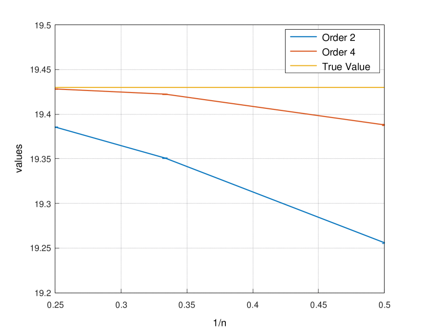
(a) Values plot

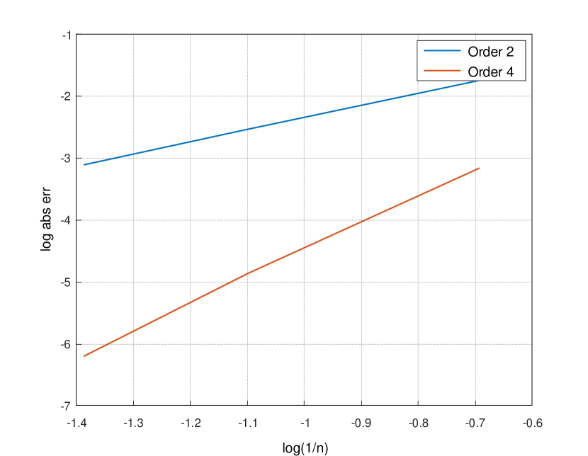
(b) Log-log plot

Figure 1. Test function: $f(x,y)=(K-e^{x})^{+}$. Parameters: $S_{0}=e^{x}=100$, $r=0$, $y=0.2$, $a=0.2$, $b=1$, $\sigma=0.5$, $\rho=-0.7$, $T=1$, $K=105$. Statistical precision $\varepsilon=5$e-4. Graphic (a) shows the Monte Carlo estimated values of $\hat{\mathcal{P}}^{NV,1,n}f$, $\hat{\mathcal{P}}^{NV,2,n}f$ as a function of the time step $1/n$ and the exact value. Graphic (b) draws $\log(|\hat{\mathcal{P}}^{NV,\nu,n}f-P_{T}f|)$ in function of $\log(1/n)$: the regressed slopes are 1.89 and 4.27 for the second and fourth order respectively.

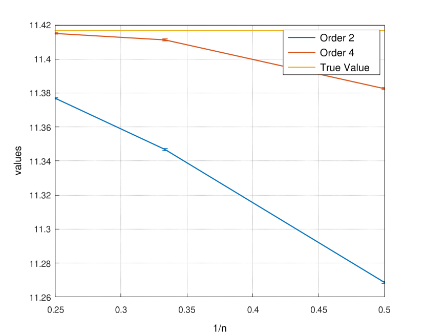
(a) Values plot

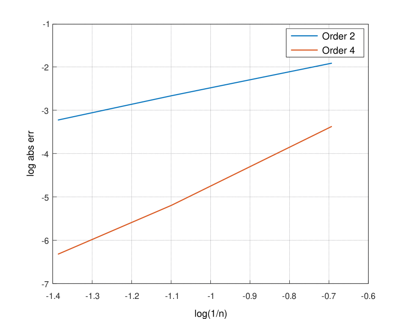
(b) Log-log plot

Figure 2. Test function: $f(x,y)=(K-e^{x})^{+}$. Parameters: $S_{0}=e^{x}=100$, $r=0$, $y=0.1$, $a=0.1$, $b=1$, $\sigma=1.0$, $\rho=-0.9$, $T=1$, $K=105$. Statistical precision $\varepsilon=5$e-4. Graphic (a) shows the Monte Carlo estimated values of $\hat{\mathcal{P}}^{Ex,1,n}f$, $\hat{\mathcal{P}}^{Ex,2,n}f$ as a function of the time step $1/n$ and the exact value. Graphic (b) draws $\log(|\hat{P}^{Ex,\nu,n}f-P_{T}f|)$ in function of $\log(1/n)$: the regressed slopes are 1.89 and 4.26 for the second and fourth order respectively.

4.2. Pricing of European and Asian options

We present in Figure 1 the convergence of the approximations $\hat{\mathcal{P}}^{NV,1,n}$ and $\hat{\mathcal{P}}^{NV,2,n}$ for the price of a European option in a case where $\sigma^{2}\leq 4a$. On the left graphic, we draw the values in function of the time step and the exact value of the option price $P_{T}f$, that can be calculated with Fourier transform techniques. On the right graphic is plotted the log error in function of the log time step: the estimated slopes are in line with the theoretical order of convergence (2 and 4), even though the test function $f(x)=(K-e^{x})_{+}$ is not as regular as required by Theorem 2.1. In Figure 2, we illustrate similarly the convergence of the approximations $\hat{\mathcal{P}}^{Ex,1,n}$ and $\hat{\mathcal{P}}^{Ex,2,n}$ for the price of a European option in a case where $\sigma^{2}\gg 4a$. Again, we observe the theoretical rates of convergence given by Theorem 2.1.

We now consider the case of Asian options, for which we need to simulate a third coordinate: $\mathcal{I}_{t}=\int_{0}^{t}S^{s,y}_{u}du=\int_{0}^{t}e^{X^{x,y}_{u}}du$. We explain how to simulate this coordinate for $\hat{P}^{Ex}$, and we do exactly the same then for $\hat{P}^{NV}$. We approximate the integral $\mathcal{I}_{t}$ by the trapezoidal rule. This gives

$$\hat{{\mathcal{I}}}^{Ex,0}_{kh_{1}}=\frac{e^{\hat{X}^{Ex,0}_{(k-1)h_{1}}}+e^{\hat{X}^{Ex,0}_{kh_{1}}}}{2}h_{1},\ 1\leq k\leq n,$$

$$\hat{{\mathcal{I}}}^{Ex,1}_{kh_{1}}=\hat{{\mathcal{I}}}^{Ex,0}_{kh_{1}},\ 0\leq k\leq\kappa,$$

$$\hat{{\mathcal{I}}}^{Ex,1}_{\kappa h_{1}+k^{\prime}h_{2}}=\frac{e^{\hat{X}^{Ex,1}_{\kappa h_{1}+(k^{\prime}-1)h_{2}}}+e^{\hat{X}^{Ex,1}_{\kappa h_{1}+k^{\prime}h_{2}}}}{2}h_{2},\ 1\leq k^{\prime}\leq n,$$

$$\hat{{\mathcal{I}}}^{Ex,1}_{kh_{1}}=\frac{e^{\hat{X}^{Ex,1}_{(k-1)h_{1}}}+e^{\hat{X}^{Ex,1}_{kh_{1}}}}{2}h_{1},\ \kappa+1<k\leq n,$$

with $\hat{I}^{Ex,0}_{0}=\hat{I}^{Ex,1}_{0}=0$. Let us mention here that the trapezoidal rule corresponds to the Strang splitting for the generator $\mathcal{L}+e^{x}\partial_{\mathcal{I}}$. Our formalism would allow to analyse the convergence rate for the Strang splitting for $\mathcal{L}+h(x)\partial_{\mathcal{I}}$, when $h$ is smooth with derivatives of polynomial growth. The exponential function does not fit this condition, and we analyse here the convergence on numerical experiments.

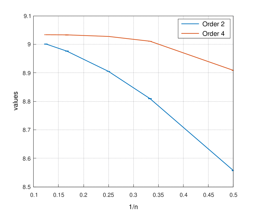
(a) Values plot

(b) Log-log plot

Figure 3. Test function: $f(x,y,i)=(K-i/T)^{+}$. Parameters: $e^{x}=100$, $r=0$, $y=0.2$, $a=0.2$, $b=2$, $\sigma=0.5$, $\rho=-0.7$, $T=1$, $K=100$. Statistical precision $\varepsilon=5$e-4. Graphic (a) shows the Monte Carlo estimated values of $\hat{\mathcal{P}}^{NV,1,n}f$, $\hat{\mathcal{P}}^{NV,2,n}f$ as a function of the time step $1/n$. Graphic (b) draws $\log(|\hat{\mathcal{P}}^{NV,\nu,2n}f-\hat{\mathcal{P}}^{NV,\nu,n}f|)$ in function of $\log(1/n)$: the regressed slopes are 1.85 and 4.30 for the second and fourth order respectively.

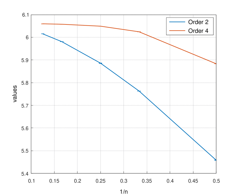
(a) Values plot

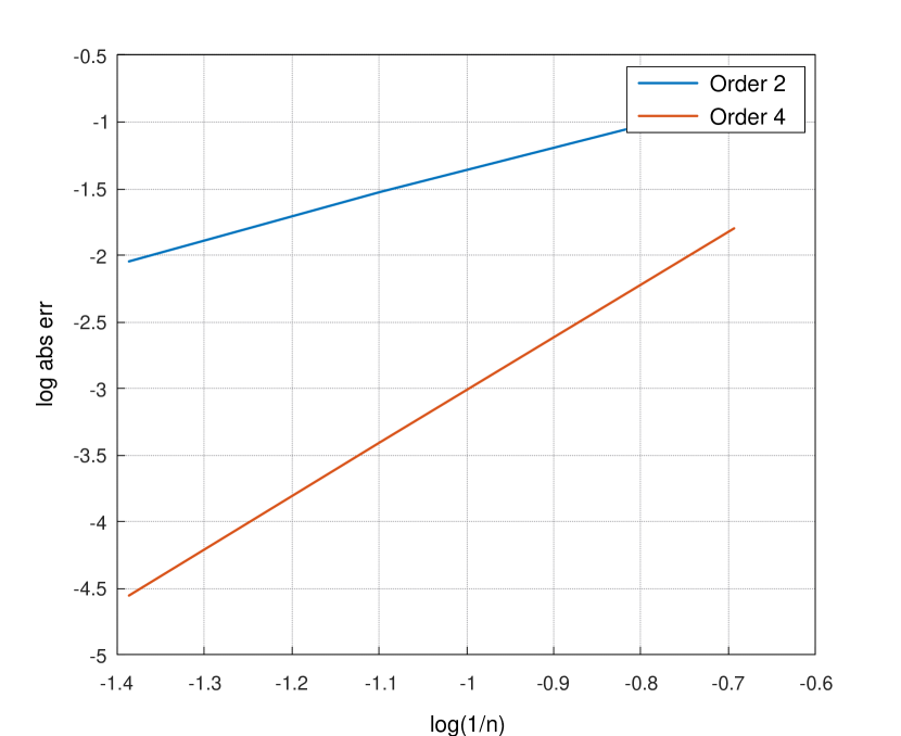
(b) Log-log plot

Figure 4. Test function: $f(x,y,i)=(K-i/T)^{+}$. Parameters: $e^{x}=100$, $r=0$, $y=0.1$, $a=0.1$, $b=1$, $\sigma=1.0$, $\rho=-0.9$, $T=1$, $K=100$. Statistical precision $\varepsilon=5$e-4. Graphic (a) shows the Monte Carlo estimated values of $\hat{\mathcal{P}}^{Ex,1,n}f$, $\hat{\mathcal{P}}^{Ex,2,n}f$ as a function of the time step $1/n$. Graphic (b) draws $\log(|\hat{\mathcal{P}}^{Ex,\nu,2n}f-\hat{\mathcal{P}}^{Ex,\nu,n}f|)$ in function of $\log(1/n)$: the regressed slopes are 1.72 and 3.98 for the second and fourth order respectively.

Figure 3 shows the convergence of the approximations $\hat{\mathcal{P}}^{NV,1,n}$ and $\hat{\mathcal{P}}^{NV,2,n}$ to calculate the Asian option price $P_{T}f={\mathbb{E}}[(K-{\mathcal{I}}_{T})^{+}]$, with $f(x,y,i)=(K-i)^{+}$. The left graphic draws the obtained value in function of the time step. This time, we do not have an exact value, and we draw in the log-log plot the logarithm of the difference between $\hat{\mathcal{P}}^{NV,\nu,2n}$ and $\hat{\mathcal{P}}^{NV,\nu,n}$. If $\hat{\mathcal{P}}^{NV,\nu,n}=P_{T}f+\frac{c}{n^{\eta}}+o(n^{-\eta})$ for some $\eta>0$, then $\log(|\hat{\mathcal{P}}^{NV,\nu,2n}-\hat{\mathcal{P}}^{NV,\nu,n}|)=\log(|c|(1-2^{-\eta}))-\eta\log(n)+o(\log(n))$, and therefore the slope of the log-log plot can be seen as an estimation of the rate of convergence. Again, we find empirical rates that are close to 2 for $\nu=1$ and 4 for $\nu=2$, which is in line with the theoretical results. The same observation holds in Figure 4 for $\hat{\mathcal{P}}^{Ex,\nu,n}$ in a case where $\sigma^{2}\geq 4a$.

4.3. Estimators variance and schemes coupling

In this paragraph, we discuss how to couple the refined path and the coarse one in order to minimize the variance of the correction term

$$n\left(f(\hat{X}^{SCH,1}_{T},\hat{Y}^{SCH,1}_{T})-f(\hat{X}^{SCH,0}_{T},\hat{Y}^{SCH,0}_{T})\right),$$

where $SCH\in\{Ex,NV\}$ indicates the scheme used. We will note

$$\mathbf{V}(n)=\text{Var}\left(n\left(f(\hat{X}^{SCH,1}_{T},\hat{Y}^{SCH,1}_{T})-f(\hat{X}^{SCH,0}_{T},\hat{Y}^{SCH,0}_{T})\right)\right).$$

While it is rather natural to take the same driving noise for the other time steps, the difficulty is to find a good coupling on $[\kappa h_{1},(\kappa+1)h_{1}]$ between the noise used on the refined time grid and the one of the coarse grid. This issue does not exist for $Y$ when it is simulated exactly, and for the Ninomiya-Victoir scheme we always take $G_{\kappa+1}=\frac{1}{\sqrt{n}}\sum_{k=1}^{n}\tilde{G}_{k}$. We therefore discuss the choice of $N_{\kappa+1}$ that is used for the simulation of $X$. We consider the two following choices:

$$N_{\kappa+1}=N^{\textup{st}}=\frac{1}{\sqrt{n}}\sum_{k=1}^{n}\tilde{N}_{k},\ \text{ or }N_{\kappa+1}=N^{\textup{av}}=\frac{\sum_{k=1}^{n}\sqrt{\hat{Y}^{SCH,1}_{\kappa h_{1}+(k-1)h_{2}}+\hat{Y}^{SCH,1}_{\kappa h_{1}+kh_{2}}}\tilde{N}_{k}}{\sqrt{\sum_{k=1}^{n}\hat{Y}^{SCH,1}_{\kappa h_{1}+(k-1)h_{2}}+\hat{Y}^{SCH,1}_{\kappa h_{1}+kh_{2}}}}.$$

Note that $N^{\textup{av}}\sim\mathcal{N}(0,1)$, since the normal variables $\tilde{N}_{k}$, $1\leq k\leq n$, are independent of the $Y$ component. This second choice is also rather natural since it weights each normal variable with the corresponding volatility on each fine time-step. A similar coupling has been proposed by Zheng [20] in a context of Multi-Level Monte-Carlo for the Heston model.

Besides this choice of coupling, we also consider another scheme for the Heston model. In fact, an alternative of Strang’s scheme is to introduce a Bernoulli random variable of parameter $1/2$ that selects which scheme is used first. We want to see if this additional random variable has an incidence on the variance of the correcting term. This scheme is given by

$$\hat{X}^{SCH,x,y}_{t}=x+(r-\frac{\rho}{\sigma}a)t+\frac{\rho}{\sigma}(\hat{Y}^{y}_{t}-y)+(\frac{\rho}{\sigma}b-\frac{1}{2})\frac{y+\hat{Y}^{y}_{t}}{2}t+\sqrt{y+B(1-\rho^{2})(\hat{Y}^{SCH,y}_{t}-y)t}N,$$

where $N\sim\mathcal{N}(0,1)$ and $B\sim\mathcal{B}(1/2)$ is an independent Bernoulli random variable. The random variable $\hat{Y}^{SCH,y}_{t}$ is either equal to $Y^{y}_{t}$ for $SCH=Ex$ or to $\hat{Y}^{y}_{t}$ for $SCH=NV$. This scheme has been used in the numerical experiments of [7] and is indicated with ”Bernoulli” in the following tables.

Scheme	Coupling	$n=2$	$n=4$	$n=8$	$n=16$	$n=32$
$NV$	$N^{\textup{st}}$	12.13	18.48	21.85	23.56	24.41
		(0.01)	(0.01)	(0.01)	(0.02)	(0.02)
$NV$	$N^{\textup{av}}$	8.31	9.08	8.91	8.70	8.57
		(0.01)	(0.01)	(0.01)	(0.01)	(0.01)
$NV$, Bernoulli	$N^{\textup{st}}$	33.27	41.96	46.14	48.27	49.37
		(0.02)	(0.03)	(0.03)	(0.04)	(0.04)
$NV$, Bernoulli	$N^{\textup{av}}$	25.11	28.55	30.74	32.13	32.85
		(0.02)	(0.02)	(0.03)	(0.03)	(0.03)
$Ex$	$N^{\textup{st}}$	30.19	30.19	28.09	26.74	26.02
		(0.02)	(0.02)	(0.02)	(0.02)	(0.02)
$Ex$	$N^{\textup{av}}$	26.35	20.80	15.17	11.88	10.18
		(0.01)	(0.01)	(0.01)	(0.01)	(0.01)

Table 1. Variance $\mathbf{V}(n)$ estimated with $10^{8}$ samples, the 95% confidence precision is indicated below in parentheses. Test function: $f(x,y)=(K-e^{x})^{+}$. Parameters: $e^{x}=100$, $r=0$, $x=0.2$, $a=0.2$, $b=1.0$, $\sigma=0.5$, $\rho=-0.7$, $T=1$, $K=105$.

Scheme	Coupling	$n=2$	$n=4$	$n=8$	$n=16$	$n=32$
$Ex$	$N^{\textup{st}}$	38.69	39.51	36.96	35.23	34.32
		(0.03)	(0.03)	(0.03)	(0.03)	(0.03)
$Ex$	$N^{\textup{av}}$	32.49	26.01	19.16	15.20	13.17
		(0.02)	(0.02)	(0.02)	(0.01)	(0.01)
$Ex$, Bernoulli	$N^{\textup{st}}$	65.66	68.93	66.95	65.47	65.01
		(0.04)	(0.05)	(0.05)	(0.05)	(0.05)
$Ex$, Bernoulli	$N^{\textup{av}}$	61.04	57.45	50.98	47.03	45.12
		(0.04)	(0.04)	(0.04)	(0.04)	(0.04)

Table 2. Variance $\mathbf{V}(n)$ estimated with $10^{8}$ samples, the 95% confidence precision is indicated below in parentheses. Test function: $f(x,y)=(K-e^{x})^{+}$. Parameters: $S_{0}=100$, $r=0$, $x=0.1$, $a=0.1$, $b=1.0$, $\sigma=1.0$, $\rho=-0.9$, $T=1$, $K=105$.

We have reported in Tables 1 and 2 the variance of the correcting term for the different schemes, the two different choices for $N_{\kappa+1}$ and different values of $n$. Table 1 reports a case with $\sigma^{2}\leq 4a$ where the Ninomiya-Victoir scheme is well defined, while Table 2 reports a case with $\sigma^{2}>4a$. In both cases, we have taken the example of a European Put option. In both tables, we observe that the scheme using a Bernoulli random variable has a correcting term of higher variance. Besides, it requires to simulate one more random variable. Thus, the schemes based on the Strang composition are better suited with the convergence acceleration using random grids.

We now comment the coupling of the schemes. In all our experiments, the coupling using $N^{\textup{av}}$ gives a lower variance than the one using $N^{\textup{st}}$. Besides, we observe that the gain factor between the two choices is increasing with $n$. We have a gain factor of $\frac{24.41}{8.57}\approx 2.85$ in Table 1 for the Ninomiya-Victoir scheme and $n=32$, and of $2.32$ in Table 2 for the scheme $Ex$ with $n=16$. As a consequence, we recommend the use of $N^{\textup{av}}$ to couple the schemes on the coarse and fine grids.

4.4. Towards higher order approximations of Rough Heston process

In this last paragraph, we propose to investigate numerically the approximations with random grids in the case of the rough Heston model. We first recall that the rough Heston model proposed by El Euch and Rosenbaum [14] is given by $S_{t}=e^{X^{x,y}_{t}}$, where

$$X^{x,y}_{t} =x+\int_{0}^{t}\left(r-\frac{1}{2}Y^{y}_{u}\right)du+\int_{0}^{t}\sqrt{Y^{y}_{u}}(\rho dW_{u}+\sqrt{1-\rho^{2}}dB_{u}),$$ (4.1)

$$Y^{y}_{t} =y+\int_{0}^{t}K(t-u)(a-bY^{y}_{u})du+\int_{0}^{t}K(t-u)\sigma\sqrt{Y^{y}_{u}}dW_{u},$$ (4.2)

where $K$ is the fractional kernel given by

$$K(t)=\frac{t^{H-1/2}}{\Gamma(H+1/2)}$$ (4.3)

with Hurst parameter $H\in(0,1/2)$. The convolution through the kernel $K$ in (4.2) introduces a dependence of the volatility $Y$ on the past, and the process $(X,Y)$ is not Markovian. Despite this, it is possible to find a process in larger dimension that is Markovian and approximates the rough process well. It is well known (see e.g. Alfonsi and Kebaier [6, Proposition 2.1]) that if we replace the rough kernel $K$ in (4.2) by a discrete completely monotone kernel

$$\tilde{K}(t)=\sum_{k=1}^{d}\gamma_{k}e^{-\rho_{k}t},\qquad\gamma_{k},\rho_{k}\geq 0,\,k\in\{1,\ldots,d\},$$ (4.4)

then the solution of the Stochastic Volterra Equation

$$\tilde{Y}_{t}=y+\int_{0}^{t}\tilde{K}(t-u)(a-b\tilde{Y}^{y}_{u})du+\int_{0}^{t}\tilde{K}(t-u)\sigma\sqrt{\tilde{Y}^{y}_{u}}dW_{u},$$ (4.5)

is given by $\tilde{Y}_{t}=y+\sum_{k=1}^{d}\gamma_{k}\tilde{Y}^{k}_{t}$, where $\tilde{\mathbf{Y}}=(\tilde{Y}^{1},\ldots,\tilde{Y}^{d})$ solves the SDE in ${\mathbb{R}}^{d}$:

$$\tilde{Y}^{k}_{t}=-\rho_{k}\int_{0}^{t}\tilde{Y}^{k}_{u}du+\int_{0}^{t}(a-b\tilde{Y}_{u})du+\int_{0}^{t}\sigma\sqrt{\tilde{Y}_{u}}dW_{u},\quad k\in\{1,\ldots,d\},t\geq 0.$$ (4.6)

We want to build a second order scheme for (4.6) along with

$$\tilde{X}_{t}=x+\int_{0}^{t}(r-\frac{1}{2}\tilde{Y}_{u})du+\int_{0}^{t}\sqrt{\tilde{Y}_{u}}(\rho dW_{u}+\sqrt{1-\rho^{2}}dB_{u}).$$

This multifactor model has been first developed by Abi Jaber and El Euch [1] and can be seen under a suitable choice of $\tilde{K}(t)=\sum_{k=1}^{d}\gamma_{k}e^{-\rho_{k}t}$ as an approximation of the rough Heston model.

We present here a second order approximation scheme for the couple $(\tilde{X},\tilde{Y})$ that preserve the positivity of $\tilde{Y}$ as proved by Alfonsi in [4, Theorem 4.2 and Subsection 4.3]. The infinitesimal generator of the $d+1$ dimensional process $(\tilde{X},\tilde{\mathbf{Y}})$ is given by

$${\mathcal{L}}f(x,{\mathbf{y}})=(r-\frac{1}{2}y^{\prime})\partial_{x}f(x,{\mathbf{y}})+\sum_{k=1}^{d}(a-\rho_{k}y_{k}-by^{\prime})\partial_{y_{k}}f(x,{\mathbf{y}})\\ +\frac{1}{2}\partial_{x}^{2}f(x,{\mathbf{y}})+\sum_{k=1}^{d}2\rho\sigma\partial_{x}\partial_{y_{k}}f(x,{\mathbf{y}})+\frac{1}{2}\sum_{k,l=1}^{d}\sigma^{2}y^{\prime}\partial_{y_{k}}\partial_{y_{l}}f(x,{\mathbf{y}}),$$ (4.7)

where ${\mathbf{y}}=(y_{1},\ldots,y_{d})$ and $y^{\prime}=y+\sum_{j=1}^{d}\gamma_{j}y_{j}$. We use the following splitting ${\mathcal{L}}={\mathcal{L}}_{1}+{\mathcal{L}}_{2}$, where ${\mathcal{L}}_{1}f=-\sum_{k=1}^{d}\rho_{k}y_{k}\partial_{y_{k}}f$ is the infinitesimal generator associated to

$$dX_{t} =0,$$ (4.8)

$$dY^{k}_{t} =-\rho_{k}Y^{k}_{t}dt,\qquad k\in\{1,\ldots,d\},$$

and ${\mathcal{L}}_{2}$ is associated to

$$dX_{t} =(r-\frac{1}{2}Y_{t})d_{t}+\sqrt{Y_{t}}(\rho dW_{t}+\sqrt{1-\rho^{2}}dB_{t}),$$ (4.9)

$$dY^{k}_{t} =(a-bY_{t})dt+\sigma\sqrt{Y_{t}}dW_{t},\text{ with }Y_{t}=y+\sum_{k=1}^{d}\gamma_{k}Y^{k}_{t}\quad k\in\{1,\ldots,d\}.$$

The linear ODE (4.8) has the exact solution

$$\psi_{1}(t,x,{\bf y})=(x,{\bf y}_{t}),\text{ with }{\bf y}_{t}=(y_{1}e^{-\rho_{1}t},\ldots,y_{d}e^{-\rho_{d}t}).$$ (4.10)

From (4.9), we obtain that $(X_{t},Y_{t})$ satisfies the following log-Heston SDEs

$$X_{t} =x+\int_{0}^{t}(r-\frac{1}{2}Y_{u})d_{t}+\int_{0}^{t}\sqrt{Y_{u}}(\rho dW_{u}+\sqrt{1-\rho^{2}}dB_{u}),$$ (4.11)

$$Y_{t} =y^{\prime}+\int_{0}^{t}K(0)(a-bY_{u})du+\int_{0}^{t}K(0)\sigma\sqrt{Y_{u}}dW_{u},$$

and $dY^{k}_{t}=\frac{1}{K(0)}dY_{t}$ (note that $K(0)=\sum_{j=1}^{d}\gamma_{j}$). So, having a second order scheme $(\hat{X}^{x,y^{\prime}}_{t},\hat{Y}^{y^{\prime}}_{t})$ for $(X_{t},Y_{t})$, we can build a second order scheme for (4.9) by

$$(\hat{X}^{x,y}_{t},\hat{Y}^{1,y}_{t},\dots,\hat{Y}^{1,y}_{t})=(\hat{X}^{x,y^{\prime}}_{t},A_{\mathbf{y}}(\hat{Y}^{y^{\prime}}_{t})),$$ (4.12)

where

$$A_{\mathbf{y}}(z)=\left(y_{1}+\frac{z-y^{\prime}}{K(0)},\ldots,y_{d}+\frac{z-y^{\prime}}{K(0)}\right).$$ (4.13)

In the end, we use again the Strang composition to get the second order scheme for (4.7) starting from $(x,{\bf y})$ and time-step $t>0$:

$$\psi_{1}\left(t/2,\hat{X}^{x,y^{\prime}_{t/2}}_{t},A_{{\mathbf{y}}_{t/2}}(\hat{Y}^{y^{\prime}_{t/2}}_{t})\right),$$ (4.14)

where $y^{\prime}_{t/2}=y+\sum_{j=1}^{d}\gamma_{j}y_{j}e^{-\rho_{j}t/2}$.

Now that we have defined the approximation scheme (4.14) for the multifactor Heston model, we want to use it to test numerically the convergence acceleration provided by the random grids. The construction of the estimators is identical to the one of $\hat{\mathcal{P}}^{NV,1,n}$ and $\hat{\mathcal{P}}^{NV,2,n}$ in Subsection 4.1 and we do not reproduce it here. Also, by a slight abuse of notation, we still denote by $\hat{\mathcal{P}}^{NV,1,n}$ and $\hat{\mathcal{P}}^{NV,2,n}$ these estimators that are well defined $\tilde{K}(0)\sigma^{2}<4a$. Unfortunately, there does not exist yet – up to our knowledge – efficient exact simulation method for the multifactor Cox-Ingersoll-Ross process. It it were the case, we could then define the corresponding estimators $\hat{\mathcal{P}}^{Ex,1,n}$ and $\hat{\mathcal{P}}^{Ex,2,n}$ exactly as in Subsection 4.1, for any $\sigma>0$. Here, we thus present only simulation in the case $\tilde{K}(0)\sigma^{2}<4a$. These simulations are intended to be a first attempt to get higher order approximations of the multifactor Heston model. We let the case $\tilde{K}(0)\sigma^{2}>4a$ as well as theoretical proofs of convergence in this model for future studies.

Multi exponential approximations of the rough kernel are available in literature, see e.g. Abi Jaber, El Euch [1] and Alfonsi, Kebaier [6]. In our simulation we will use the algorithm BL2 suggested by Bayer and Breneis in [10], that optimizes the ${\mathbb{L}}^{2}([0,T])$-error between $K$ and $\tilde{K}$ while limiting high values of $\rho_{k}$. In particular, we will use the approximate BL2 Kernel with $d=3$ exponential factors, that has been proven to approximate a whole volatility surface of rough Heston call prices with approximately 1% of maximal relative error [10, Table 4, third column]. When the Hurst parameter $H=0.1$ the nodes and weights are resumed following table

$\rho_{1}=0.08399474$	$\rho_{2}=5.64850577$	$\rho_{3}=118.00624702$
$\gamma_{1}=0.80386099$	$\gamma_{2}=1.60786461$	$\gamma_{3}=8.80775525$

We consider European put option prices and present in Figure 5(a) a plot of the values of $\hat{\mathcal{P}}^{NV,1,n}f$ and $\hat{P}^{NV,2,n}f$ as a function of the time step with the exact value obtained by Fourier techniques. In Figure 5(b), we draw a log-log plot to quantify the order of convergence. First, we observe that we obtain a much larger bias than in our previous numerical experiments for the Heston process, Figure 2(a). This is mainly due to the map $\psi_{1}$ that has a relatively large nodes, namely $\rho_{2}$ and especially $\rho_{3}$. The contribution of these exponential factors in the dynamics of the scheme gets more important when the time step is sufficiently small. However, even if the bias is more important, the speed of convergence are still in line with the theoretical ones. The regressed slopes for $\hat{\mathcal{P}}^{NV,1,n}f$ and $\hat{P}^{NV,2,n}f$ are respectively 1.89 and 3.98, showing that the scheme is indeed a second-order scheme and that the boosting technique with random grids works again in this case.

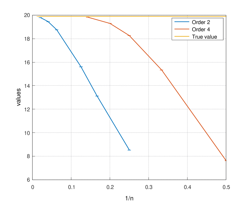
(a) Values plot

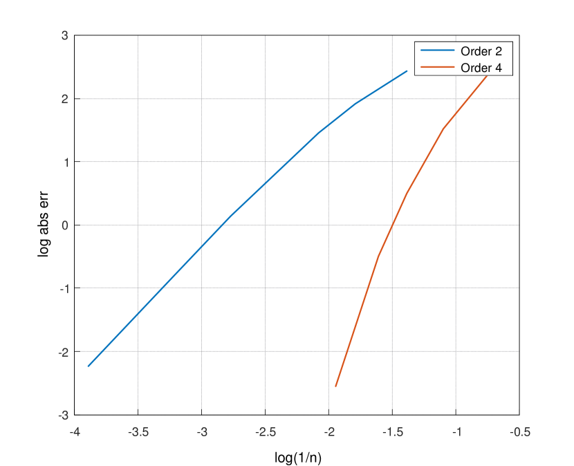
(b) Log-log plot

Figure 5. Test function: $f(x,y)=(K-e^{x})^{+}$. Parameters: $S_{0}=e^{x}=100$, $r=0$, $y=0.1$, $a=0.3$, $b=1$, $\sigma=0.1$, $\rho=-0.7$, $T=1$, $K=105$. Statistical precision $\varepsilon=2$e-3. Graphic (a) shows the Monte Carlo estimated values of $\hat{\mathcal{P}}^{NV,1,n}f$, $\hat{\mathcal{P}}^{NV,2,n}f$ as a function of the time step $1/n$ and the exact option value. Graphic (b) draws $\log(|\hat{\mathcal{P}}^{NV,\nu,n}f-P_{T}f|)$ in function of $\log(1/n)$: the regressed slopes are 1.89 and 3.98 for the second and fourth order respectively.

References

• [1] E. Abi Jaber and O. El Euch. Multifactor approximation of rough volatility models. SIAM journal on financial mathematics, 10(2):309–349, 2019.
• [2] A. Alfonsi. High order discretization schemes for the CIR process: application to affine term structure and Heston models. Math. Comp., 79(269):209–237, 2010.
• [3] A. Alfonsi. Affine diffusions and related processes: simulation, theory and applications, volume 6 of Bocconi & Springer Series. Springer, Cham; Bocconi University Press, Milan, 2015.
• [4] A. Alfonsi. Nonnegativity preserving convolution kernels. application to stochastic volterra equations in closed convex domains and their approximation. arXiv preprint arXiv:2302.07758, 2023.
• [5] A. Alfonsi and V. Bally. A generic construction for high order approximation schemes of semigroups using random grids. Numer. Math., 148(4):743–793, 2021.
• [6] A. Alfonsi and A. Kebaier. Approximation of stochastic volterra equations with kernels of completely monotone type. Mathematics of Computation, 93(346):643–677, 2024.
• [7] A. Alfonsi and E. Lombardo. High order approximations of the Cox–Ingersoll–Ross process semigroup using random grids. IMA Journal of Numerical Analysis, page drad059, 2023.
• [8] M. Altmayer and A. Neuenkirch. Discretising the Heston model: an analysis of the weak convergence rate. IMA J. Numer. Anal., 37(4):1930–1960, 2017.
• [9] L. Andersen. Simple and efficient simulation of the Heston stochastic volatility model. Journal of Computational Finance, 11(3), 2008.
• [10] C. Bayer and S. Breneis. Weak markovian approximations of rough heston. arXiv preprint arXiv:2309.07023, 2023.
• [11] M. Briani, L. Caramellino, and G. Terenzi. Convergence rate of Markov chains and hybrid numerical schemes to jump-diffusion with application to the Bates model. SIAM J. Numer. Anal., 59(1):477–502, 2021.
• [12] M. Broadie and O. Kaya. Exact simulation of stochastic volatility and other affine jump diffusion processes. Oper. Res., 54(2):217–231, 2006.
• [13] C. Cuchiero, M. Keller-Ressel, and J. Teichmann. Polynomial processes and their applications to mathematical finance. Finance Stoch., 16(4):711–740, 2012.
• [14] O. El Euch and M. Rosenbaum. The characteristic function of rough heston models. Mathematical Finance, 29(1):3–38, 2019.
• [15] P. Glasserman and K.-K. Kim. Gamma expansion of the Heston stochastic volatility model. Finance Stoch., 15(2):267–296, 2011.
• [16] S. L. Heston. A closed-form solution for options with stochastic volatility with applications to bond and currency options. Rev. Financ. Stud., 6(2):327–343, 1993.
• [17] R. Lord, R. Koekkoek, and D. Van Dijk. A comparison of biased simulation schemes for stochastic volatility models. Quant. Finance, 10(2):177–194, 2010.
• [18] S. Ninomiya and N. Victoir. Weak approximation of stochastic differential equations and application to derivative pricing. Appl. Math. Finance, 15(1-2):107–121, 2008.
• [19] D. Talay and L. Tubaro. Expansion of the global error for numerical schemes solving stochastic differential equations. Stochastic Anal. Appl., 8(4):483–509 (1991), 1990.
• [20] C. Zheng. Multilevel Monte Carlo using approximate distributions of the CIR process. BIT, 63(2):Paper No. 38, 39, 2023.