Exact and asymptotic dissipative spectral form factor for elliptic Ginibre unitary ensemble

Abstract

The dissipative spectral form factor (DSFF) has recently emerged as a diagnostic tool for assessing non-integrability or chaos in non-Hermitian systems. It extends the concept of the spectral form factor (SFF), a widely used measure for similar investigations in Hermitian systems. In this study, we concentrate on the elliptic Ginibre unitary ensemble (eGinUE), which interpolates between the non-Hermitian limit of Ginibre unitary ensemble (GinUE) and the Hermitian limit of Gaussian unitary ensemble (GUE) by varying a symmetry parameter. We derive exact finite-dimension expression and large-dimension approximation for the DSFF of eGinUE. A key finding of this work is a compelling “scaling relationship” between the DSFF of eGinUE and that of the GUE or GinUE. This scaling relationship also reveals a previously unobserved connection between the DSFF of GinUE and the SFF of GUE. The DSFF for eGinUE displays a dip-ramp-plateau structure in the GinUE and GUE limits, as well as in the crossover region, with differences in time scales that are well-explained by the aforementioned scaling relationship. Additionally, depending on the symmetry regime within the crossover, we provide various estimates for the Thouless time ($T_{\mathrm{Th}}$) and Heisenberg time ($T_{\mathrm{H}}$), which correspond to the dip-ramp and ramp-plateau transitions, respectively. Our analytical results are compared with Monte Carlo simulations of the eGinUE random matrix model, showing excellent agreement.

I Introduction

Among the various measures employed to examine the spectral behavior of different systems and reveal information about their integrable or chaotic nature, the spectral form factor (SFF) is particularly powerful. In its basic form, the SFF is defined as the Fourier transform of the two-level correlation function with respect to the energy difference, although generalizations have also been proposed. While the concept of utilizing the Fourier transform to analyze spectral correlations is relatively old [1], it has gained significant attention in recent years due to the insights it provides in many-body physics [2]. One examines the SFF as a function of the time variable, which is conjugate to the energy difference. For random matrices, the SFF exhibits a dip-ramp-plateau shape, which serves as a diagnostic for detecting non-integrability or chaos [3, 4, 5, 6, 7, 8]. Specifically, when comparing with the SFF of a complex or chaotic system, the behavior after the Thouless time ($T_{\mathrm{Th}}$) [9] is of interest, where the ramp feature is observed. This indicates the onset of random matrix behavior, eventually saturating to the plateau region at the Heisenberg time ($T_{\mathrm{H}}$) [10], which corresponds to the scale of mean-level spacing in the energy domain. The SFF has been found to remain robust even in noisy environments [11, 12, 13, 14, 15]. For these reasons, it has been applied to a plethora of systems, including quantum spin chains, various disordered systems, and topological insulators [16, 17, 18, 19, 20].

Conventionally, the spectral form factor (SFF) has been applied to Hermitian systems, which naturally have a real eigenspectrum. However, with the recent surge of interest in non-Hermitian physics [21, 22, 23, 24, 25, 26, 27, 28, 29, 30, 31, 32, 33, 34, 35, 36, 37, 38], as well as non-Hermitian RMT [39, 40, 41], there is a growing need to identify suitable platforms and diagnostics for probing non-Hermitian systems, including open systems. This increased focus has led to the generalization of certain spectral traits for non-Hermitian Hamiltonians to better understand non-integrability and chaos [42, 43, 44]. Alongside the generalization of short-range correlations, the concept of the dissipative spectral form factor (DSFF) has extended the notion of spectral correlations at all scales to the complex plane [45, 46, 47]. The DSFF captures universal signatures of dissipative quantum chaos, and exact solutions for it within RMT are now known for both dissipative and integrable systems [48, 49, 48].

In this study, we derive finite-dimension exact as well as large-dimension approximate expressions for the DSFF of elliptic Ginibre unitary ensemble (eGinUE) [50, 51]. This ensemble interpolates between the two extreme of the Ginibre unitary ensemble (GinUE) [39] and the Gaussian unitary ensemble (GUE) [52, 53], as a symmetry parameter is varied. Introduced in Refs. [54, 55], the eGinUE was initially examined in the context of local correlation functions [56]. It serves as a natural random matrix ensemble for modeling systems experiencing Hermiticity breaking. In addition to providing both exact and approximate solutions, we reveal a surprisingly simple exact “scaling” relation between the DSFF of the eGinUE and the SFF of the GUE. This relation holds for all matrix-dimensions and permissible values of the symmetry parameter. Consequently, it allows one to map all known results for the SFF of the GUE onto the corresponding DSFF results for the eGinUE, and hence GinUE. By utilizing large-dimension approximations for DSFF, we also provide estimates for $T_{\mathrm{Th}}$ and $T_{H}$ that can be applied depending on the degree of Hermiticity breaking in the eGinUE model.

The rest of the paper is organized as follows. In Sec. II, we review the quantity of interest, namely the dissipative spectral form factor (DSFF), and related quantities. Section III describes the eGinUE model that we analyze. In Sec. IV, we discuss the DSFF for eGinUE, deriving its exact finite-dimension analytical expression as well as the associated large-dimension approximations. Finally, in V, we conclude with a brief summary of our work. Outlines of some derivations are provided in the Appendices.

II Spectral form factor (SFF) and dissipative spectral form factor (DSFF)

In this section, we review the quantity of interest, namely the dissipative spectral form factor. However, prior to that, we recall the definition of the spectral form factor. Consider an ensemble comprising sets of real eigenspectra $\{E_{1},...,E_{D}\}$, then in its basic form, the ensemble averaged SFF is given by

$${}\mathrm{SFF}(t)=\left\langle\left|\sum_{n=1}^{D}e^{itE_{n}}\right|^{2}\right\rangle=\left\langle\sum_{n,m=1}^{D}e^{it(E_{n}-E_{m})}\right\rangle,$$ (1)

where ‘$t$’ is the time variable and $\langle{\cdot\rangle}$ represents the ensemble average. The SFF defined in Eq. (1) can be seen as a special case $g(0,t)$ of the quantity $g(\beta,t)$ which is defined in terms of the analytic continuation of thermal partition function $Z(\beta)$ [57, 58], i.e.,

$${}g(\beta,t) \equiv|Z(\beta+it)|^{2}$$

$$=\sum_{n,m=1}^{D}e^{-\beta(E_{n}+E_{m})+it(E_{n}-E_{m})},$$ (2)

where $\beta$ is the inverse temperature. Also, the Boltzmann constant $k_{B}$ and Planck’s constant $\hbar$ have been set to unity. The spectral form factor $\mathrm{SFF}(t)$ generally exhibits complex temporal behavior since it involves sum incorporating different energy differences $(E_{n}-E_{m})$.

A generalization of SFF to the non-Hermitian systems, which involve complex eigenvalues in general, has been proposed in Ref. [48]. As pointed out above, it has been dubbed dissipative spectral form factor (DSFF) and defined as follows. Consider an ensemble of a set of complex spectra $\{z_{1},...,z_{D}\}$, where $z_{n}=x_{n}+iy_{n};x_{n},y_{n}\in\mathbb{R}$. These complex eignvalues may belong to a generic $D$-dimensional non-Hermitian Hamiltonian. The ensemble averaged and scaled DSFF is then defined as [48],

$$\mathcal{F}(t,s) =\frac{1}{D}\left\langle\sum_{n,m=1}^{D}e^{it(x_{n}-x_{m})+is(y_{n}-y_{m})}\right\rangle$$

$$=1+\frac{1}{D}\left\langle\sum_{n,m=1\atop(n\neq m)}^{D}e^{it(x_{n}-x_{m})+is(y_{n}-y_{m})}\right\rangle.$$ (3)

Here, $t$ and $s$ are two generalized time variables conjugate to the real $(x_{n}-x_{m})$ and imaginary $(y_{n}-y_{m})$ parts of the difference between two eigenvalues, $z_{n}$ and $z_{m}$. When the spectrum is real, the SFF($t$) of Eq. (1) is recovered from $\mathcal{F}(t,s)$ as a function of $t$ for all finite $s$. One may express DSFF in terms of the complex time variable, $T=t+is\equiv|T|e^{i\varphi}$ as [48],

$${}\mathcal{F}(T,T^{*})=\frac{1}{D}\left\langle\left|\sum_{n=1}^{D}e^{i(z_{n}T^{*}+z_{n}^{*}T)/2}\right|^{2}\right\rangle.$$ (4)

In Ref. [48], the authors have established that analogous to the SFF for closed systems, the DSFF also exhibits a dip-ramp-plateau behavior as a function of $|T|$, for the standard non-Hermitian Gaussian ensembles, i.e., the Ginibre orthogonal, unitary, and symplectic ensembles (GinOE, GinUE, GinSE). For the GinUE, the DSFF turns out to be independent of $\varphi$, which is a consequence of the rotationally symmetric spectrum of GinUE. On the other hand, for GinOE and GinSE, one does observe the angular dependence due to the occurrence of real and complex-conjugate pairs of eigenvalues. The precise DSFF for Poissonian case, which regards the uncorrelated complex spectrum as the minimal model of integrable systems, is also given in Ref. [48].

III Elliptic Ginibre Unitary Ensemble (eGinUE)

Elliptic Ginibre random matrix ensemble was conceived in order to model the crossover between Hermitian random matrices [54], characterized by the Wigner-Dyson statistics of real eigenvalues, and non-Hermitian random matrices, which result in complex eigenvalues as initially studied by Ginibre [39]. This crossover is facilitated by a symmetry-breaking parameter. As this parameter is varied; the eigenvalues transition from the complex plane (non-Hermitian case) to the real line (Hermitian case), resulting in a corresponding change in spectral correlations. The eGinUE can be physically interpreted in terms of a two-dimensional one-component plasma in a quadrupolar field [59, 52], which extends Dyson’s log-gas interpretation for the eigenvalues of Hermitian random matrix ensembles. Recently, higher-dimensional generalizations of the eGinUE have also been considered, with studies analyzing its local and global spectral statistics [60].

The non-Hermitian random matrix belonging to eGinUE can be decomposed in terms of its Hermitian and skew-Hermitian parts [54], viz.,

$${}\textbf{H}=\textbf{S}+i\textbf{A}.$$ (5)

Here S and A are $(D\times D)$-dimensional statistically independent Hermitian matrices chosen from GUE with probability densities,

$$\mathcal{P}_{S}(\textbf{S})=2^{-\frac{D}{2}}\left(\frac{2D}{\pi(1+\tau)v^{2}}\right)^{\frac{D^{2}}{2}}e^{-\frac{D}{(1+\tau)v^{2}}\mathrm{tr}\textbf{S}^{2}},$$ (6)

and

$$\mathcal{P}_{A}(\textbf{A})=2^{-\frac{D}{2}}\left(\frac{2D}{\pi(1-\tau)v^{2}}\right)^{\frac{D^{2}}{2}}e^{-\frac{D}{(1-\tau)v^{2}}\mathrm{tr}\textbf{A}^{2}},$$ (7)

respectively. In Eq. (5), essentially, the symmetry of the “primary” Hamiltonian S is broken by the “perturbing” Hamiltonian A, and the degree of this symmetry breakage is being regulated by the crossover parameter $\tau$. The additional parameter $v^{2}(>0)$ fixes scale of the problem. With the aid of distributions of ${\bf S}$ and ${\bf A}$, one can obtain the probability density function for ${\bf H}$ describing the eGinUE as,

$${}\mathcal{P}_{H}(\textbf{H})=\left(\frac{D}{\pi v^{2}\sqrt{1-\tau^{2}}}\right)^{D^{2}}e^{-\frac{D}{(1-\tau^{2})v^{2}}\mathrm{tr}(\textbf{H}\textbf{H}^{\dagger}-\tau\mathrm{Re}(\textbf{H}^{2}))},$$ (8)

where $\mathrm{Re}(X)$ represents the real part of $X$. In the limits of $\tau\to 0$ and $\tau\to 1$, we obtain GinUE and GUE, respectively, with the density function for ${\bf H}$ reducing to $\mathcal{P}_{H}(\textbf{H})\propto e^{-\frac{D}{v^{2}}\mathrm{tr}{\bf H}{\bf H}^{\dagger}}$ and $\mathcal{P}_{H}(\textbf{H})\propto e^{-\frac{D}{2v^{2}}\mathrm{tr}{\bf H}^{2}}$. The term “elliptic” has to do with the fact that as $D\rightarrow\infty$, the eigenvalues $(z_{n}=x_{n}+iy_{n};x_{n},y_{n}\in\mathbb{R})$ of H in bulk get confined to an ellipse in the complex plane [61, 40],

$${}\frac{x^{2}}{(1+\tau)^{2}}+\frac{y^{2}}{(1-\tau)^{2}}\leq v^{2}.$$ (9)

When $\tau=0$, the eigenvalues are distributed uniformly over the disk of radius $v$, whereas $\tau\to 1$ makes the eigenvalues collapse to the real line. In the following we set $v=1$ for the sake of simplicity.

IV Calculation and results for ${\bf eGinUE}$ DSFF

In this section, we present exact finite-dimension DSFF expression for the eGinUE as well as the corresponding large-dimension approximations. Since computation of the DSFF involves distribution of eigenvalues, our starting point relies on utilizing the results derived in Ref. [54]. Based on the distribution over the set of matrices, Eq. (8), the joint probability density $\mathcal{P}_{D}(\{z\})$ of the complex eigenvalues $\{z\}\equiv{z_{1},...,z_{D}}$ can be derived to be

$$\mathcal{P}_{D}(\{z\})=\frac{D^{D(D+1)/2}}{\pi^{N}(1-\tau^{2})^{D/2}(\prod_{m=1}^{D}m!)}\,\prod_{j>k}|z_{j}-z_{k}|^{2}$$

$$~{}~{}~{}~{}~{}~{}~{}\times\exp\left[\frac{-D}{(1-\tau^{2})}\sum_{l=1}^{D}\{|z_{l}|^{2}-\frac{\tau}{2}(z_{l}^{2}+z_{l}^{*2})\}\right].$$ (10)

The standard Dyson-Mehta procedure based on orthogonal polynomials then enables one to write down the $n$-eigenvalue correlation function,

$${}R_{n}(z_{1},...,z_{n})=\frac{D!}{(D-n)!}\int d^{2}z_{n+1}\cdots d^{2}z_{D}\mathcal{P}_{D}(\{z\}),$$ (11)

in terms of a determinant, viz.,

$${}R_{n}(z_{1},...,z_{n})=\text{det}[\mathcal{K}(z_{j},z_{k}^{*})]_{j,k=1}^{n},$$ (12)

where the kernel $\mathcal{K}(z_{j},z_{k}^{*})$ is given by

$$\mathcal{K}(z_{j},z_{k}^{*})=w{(z_{j})}w{(z_{k}^{*})}\sum_{n=0}^{D-1}p_{n}(z_{j})p_{n}(z_{k}^{*}),$$ (13)

with the weight function

$${}w^{2}{(z)}=\exp\left[-\frac{D}{1-\tau^{2}}\left(|z|^{2}-\frac{\tau}{2}(z^{2}+z^{*2})\right)\right].$$ (14)

The polynomials $p_{j}(z)$ are expressible in terms of scaled Hermite polynomials ($H_{j}(u)$) with complex argument [62], viz.,

$$p_{j}(z)=\frac{\sqrt{D}}{\sqrt{\pi\,j!}\,(1-\tau^{2})^{1/4}}\left(\frac{\tau}{2}\right)^{j/2}H_{j}\left(\sqrt{\frac{D}{2\tau}}\,z\right),$$ (15)

where $j=0,1,2,\ldots$. These satisfy the orthonormality relation,

$$\int d^{2}z\,w^{2}(z)p_{j}(z)p_{k}(z^{*})=\delta_{jk},$$ (16)

where $d^{2}z=|z|\,d|z|\,d(\mathrm{arg}(z))=dx\,dy$, with the integral extending over the entire complex plane. The one-eigenvalue correlation function $R_{1}(z)$, serves as the 2d-density of states, and therefore $\int d^{2}z\,R_{1}(z)=D$.

The DSFF in Eq. (II) can be computed using the two-point correlation function as,

$$\mathcal{F}(t,s)=1+\frac{1}{D}\int d^{2}z_{1}d^{2}z_{2}e^{it(x_{1}-x_{2})+is(y_{1}-y_{2})}R_{2}(z_{1},z_{2})$$

$$=1+\frac{1}{D}\int d^{2}z_{1}d^{2}z_{2}e^{it(x_{1}-x_{2})+is(y_{1}-y_{2})}\mathcal{K}(z_{1},z_{1}^{*})\mathcal{K}(z_{2},z_{2}^{*})$$

$$~{}~{}~{}~{}~{}-\frac{1}{D}\int d^{2}z_{1}d^{2}z_{2}e^{it(x_{1}-x_{2})+is(y_{1}-y_{2})}\mathcal{K}(z_{1},z_{2}^{*})\mathcal{K}(z_{2},z_{1}^{*})$$

$$\equiv\mathcal{F}_{\text{cont}}(t,s)+\mathcal{F}_{\text{dis}}(t,s)-\mathcal{F}_{\text{conn}}(t,s).$$ (17)

The three terms on the RHS of the above equation are identified as the contact ($\mathcal{F}_{\text{cont}}$), disconnected ($\mathcal{F}_{\text{dis}}$), and connected ($\mathcal{F}_{\text{conn}}$) parts of the overall DSFF, respectively. The contact part $\mathcal{F}_{\text{cont}}$ equals unity, trivially. Derivation of the the other two parts requires some rigorous algebraic calculations, which we outline in the Appendix A.

At early times $|T|\lesssim T_{\mathrm{Th}}$, the DSFF captures the energy level correlations at an energy scale significantly larger than the mean energy level spacing of the system. It exhibits a decay behavior, referred to as dip and is mainly dominated by the disconnected part of the DSFF, which presently turns out to be,

$${}\mathcal{F}_{\text{dis}}(t,s)=\frac{1}{D}e^{-\frac{(1+\tau)t^{2}}{2\,D}-\frac{(1-\tau)s^{2}}{2\,D}}\big{[}L_{D-1}^{(1)}(\mathscr{T})\big{]}^{2}.$$ (18)

Here $L_{a}^{(k)}(u)$ is the associated Laguerre polynomial and we have defined for convenience,

$$\mathscr{T}=\frac{(1+\tau)^{2}t^{2}+(1-\tau)^{2}s^{2}}{4\,D}=\frac{\eta^{2}}{D}|T|^{2},$$ (19)

with $\eta=(1/2)[(1+\tau)^{2}\cos^{2}\varphi+(1-\tau)^{2}\sin^{2}\varphi]^{1/2}$. We note that for $\tau=0$ and $\tau=1$, $\eta$ reduces to $1/2$ and $\cos\varphi$, respectively. In Eq. (18), instead of associated Laguerre polynomial, we may use Kummer confluent hypergeometric function $M(a,b,z)$ ($=\!\,_{1}F_{1}(a,b,z))$, or Tricomi confluent hypergeometric function $U(a,b,z)$ using the relation, $L_{a}^{(k)}(z)=\binom{a+k}{a}M(-a,k+1,z)=\frac{(-1)^{a}}{a!}U(-a,k+1,z)$, which holds for non-negative integer $a$, with $\binom{u}{v}$ representing the binomial coefficient.

The connected part of DSFF turns out to be,

$${}\mathcal{F}_{\text{conn}}(t,s) =\frac{1}{D}e^{-\frac{(1+\tau)t^{2}}{2\,D}-\frac{(1-\tau)s^{2}}{2\,D}}$$

$$\times\sum_{n,m=0}^{D-1}\frac{m!}{n!}\mathscr{T}^{n-m}\big{[}L_{m}^{(n-m)}(\mathscr{T})\big{]}^{2}.$$ (20)

The double sum over $n,m$ in the above equation may be separated using $n=m$ and $n>m$ (or $n<m$) parts only by using the following property of the associated Laguerre polynomials: $L_{a}^{(-k)}(z)=(-z)^{k}\frac{(a-k)!}{a!}L_{a-k}^{(k)}(z)$. The connected part dominates at the intermediate time-scale $T_{\mathrm{Th}}\lesssim|T|\lesssim T_{\mathrm{H}}$, leading to a ramp-type behavior of DSFF. This time scale is used to infer quantum chaotic behavior when examining the DSFF of complex systems. Beyond $T_{\mathrm{H}}$ the DSFF tends to saturate to a constant plateau value (of unity) governed by the contact term, $\mathcal{F}_{\mathrm{cont}}$. It should be noted that the DSFF for eGinUE depends on the combination of $t^{2}=|T|^{2}\cos^{2}\varphi$ and $s^{2}=|T|^{2}\sin^{2}\varphi$, which makes it invariant under the transformation $\varphi\to\pi\pm\varphi$. Equations (18) and (IV) constitute the first key contribution of our paper.

When one of the extreme instances, $\tau=0$, is considered, Eq. (IV) leads to the GinUE result [48, 49],

$$\mathcal{F}^{\mathrm{GinUE}}(T)=1+\frac{e^{-\frac{|T|^{2}}{2\,D}}}{D}\left[L_{D-1}^{(1)}\bigg{(}\frac{|T|^{2}}{4D}\bigg{)}\right]^{2}$$

$$-\frac{e^{-\frac{|T|^{2}}{2\,D}}}{D}\sum_{n,m=0}^{D-1}\frac{m!}{n!}\bigg{(}\frac{|T|^{2}}{4D}\bigg{)}^{n-m}\left[L_{m}^{(n-m)}\bigg{(}\frac{|T|^{2}}{4\,D}\bigg{)}\right]^{2},$$ (21)

By setting $\tau=1$, we obtain the other extreme [63],

$$\mathcal{F}^{\mathrm{GUE}}(t)=1+\frac{e^{-\frac{t^{2}}{D}}}{D}\left[L_{D-1}^{(1)}\bigg{(}\frac{t^{2}}{D}\bigg{)}\right]^{2}$$

$$-\frac{e^{-\frac{t^{2}}{D}}}{D}\sum_{n,m=0}^{D-1}\frac{m!}{n!}\left(\frac{t^{2}}{D}\right)^{n-m}\left[L_{m}^{(n-m)}\bigg{(}\frac{t^{2}}{D}\bigg{)}\right]^{2}.$$ (22)

This expression depends on $\mathrm{Re}(T)=t=|T|\cos\varphi$, which includes the $\cos\varphi$ dependency. However, this dependence just serves as the scaling of the time variable as far as GUE is concerned. In fact, the SFF expression defined by Eq. (1) for the GUE case associated with the matrix probability density $\exp(-\frac{D}{2}\mathrm{tr}{\bf H}^{2})$, can be derived using its eigenvalue correlations directly and coincides with Eq. (IV), i.e., $\mathrm{SFF}^{\mathrm{GUE}}(t)=\mathcal{F}(t,s)|_{\tau=1}$, as one would expect, the variable $t$ now being the usual real time variable used in (1).

By comparing Eqs. (IV) and (IV), we find an intriguing “scaling relationship” between the respective disconnected and connected parts, viz.,

$$\mathcal{F}^{\mathrm{GinUE}}_{\mathrm{dis,conn}}(T)=e^{\frac{-|T|^{2}}{4}}\mathcal{F}^{\mathrm{GUE}}_{\mathrm{dis,conn}}(|T|/2),$$ (23)

As a matter of fact the DSFF for the eGinUE can similarly be expressed in terms of the GUE result. We have,

$$\mathcal{F}_{\mathrm{dis,conn}}(t,s)=e^{-\frac{(1-\tau^{2})(t^{2}+s^{2})}{\sqrt{4D}}}\mathcal{F}^{\mathrm{GUE}}_{\mathrm{dis,conn}}(\sqrt{D\mathscr{T}}).$$ (24)

This expression can be considered the core result of this work. Besides being aesthetically pleasing, it is immensely powerful and reveals a deep connection between the various symmetry regimes of the eGinUE, including the extremes of the GinUE and GUE.

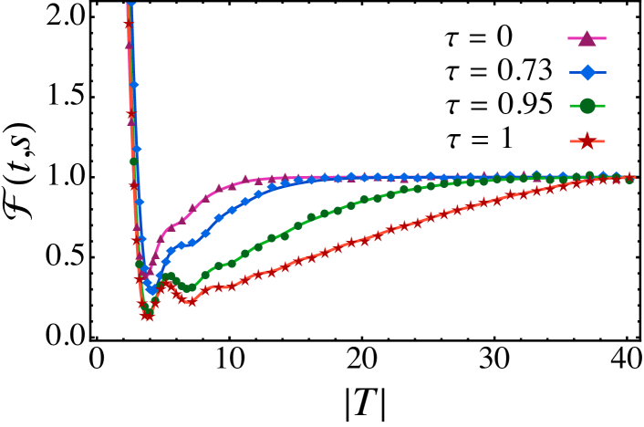
Figure 1: Plots of the eGinUE DSFF $\mathcal{F}(t,s)$ as a function of $|T|$ for $D=10$ and $\varphi=\pi/3$. The solid curves represent exact analytical results, while symbols (triangle, diamond, disk, star) are based on Monte Carlo simulations of the eGinUE matrix model. The crossover from GinUE to GUE symmetry is clearly observed with varying symmetry parameter $\tau$.

We now present large-$D$ approximations for the DSFF, which have been deduced in Appendix B. We find that the disconnected and connected parts of the DSFF of eGinUE assume the following forms, respectively,

$$\mathcal{F}_{\mathrm{dis}}(t,s) \approx\frac{1}{\mathscr{T}}\,e^{-\frac{(1-\tau^{2})(t^{2}+s^{2})}{4D}}J_{1}\big{(}2\sqrt{D\mathscr{T}}\big{)}^{2},$$ (25)

$$\mathcal{F}_{\mathrm{conn}}(t,s)\approx e^{-\frac{(1-\tau^{2})(t^{2}+s^{2})}{4D}}\mathcal{S}\big{(}\sqrt{D\mathscr{T}}\big{)}.$$ (26)

In the above, $J_{n}(u)$ is the Bessel function of order $n$, and $\mathcal{S}(u)$ is given by

$$\mathcal{S}(u)=\frac{2}{\pi}\csc^{-1}\left(\frac{2D}{\sqrt{4D^{2}-u^{2}}}\right)-\frac{u\sqrt{4D^{2}-u^{2}}}{2\pi D^{2}},$$ (27)

for $u<2D$, and $0$ for $u\geq 2D$. In the $\tau\to 0$ and $\tau\to 1$ limits, these lead to the following asymptotic results for GinUE [48] and GUE [64], respectively,

$$\mathcal{F}^{\mathrm{GinUE}}(T) \approx 1+e^{-\frac{|T|^{2}}{4\,D}}\frac{4D}{|T|^{2}}J_{1}(|T|)^{2}-e^{-\frac{|T|^{2}}{4\,D}}\mathcal{S}(|T|/2)$$

$$\approx 1+\frac{4D}{|T|^{2}}J_{1}(|T|)^{2}-e^{-\frac{|T|^{2}}{4\,D}},$$ (28)

$$\mathcal{F}^{\mathrm{GUE}}(t) \approx 1+\frac{D}{t^{2}}J_{1}(2t)^{2}-\mathcal{S}(t).$$ (29)

The asymptotic expressions for the eGInUE DSFF serve as yet another key contribution of our paper.

We now present the plots of DSFF using both our exact and approximate results. In Fig. 1, we consider $D=10,\varphi=\pi/3$ and show variation of DSFF with changing $\tau$ using the exact analytical expression as solid curves. For comparison, we also depict numerical data using symbols, obtained from the simulation of eGinUE matrix model, Eq. (5), using 10000 matrices. We can see a very good agreement. In Fig. 2, we show the comparison between the above large-$D$ approximations and simulation results for $D=125$ and $\varphi=0$, based on 5000 matrices. We can see that these approximations work remarkably well and accurately captures even the fine oscillations in the ‘dip’ region. The characteristic dip-ramp-plateau feature can be clearly observed in both Figs. 1 and 2. Moreover, in both these figures, the difference in time scales for various $\tau$ values can be understood from the relations given in Eq. (24). Equations (25) and (26) can be utilized to reveal a number of interesting facts about the Thouless time $T_{\mathrm{Th}}$, Heisenberg time $T_{H}$, and the behavior of dip and ramp of the DSFF in the large-$D$ limit, as done below.

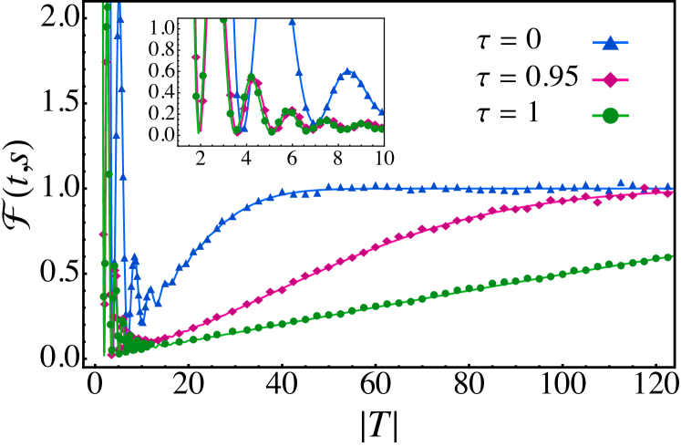
Figure 2: Plots of the eGinUE DSFF $\mathcal{F}(t,s)$ as a function of $|T|$ for $D=125$ and $\varphi=0$. The solid curves represent large-$D$ approximate analytical results, while symbols (triangle, diamond, disk) are based on Monte Carlo simulations of the eGinUE matrix model. The inset provides an enlarged view of the ‘dip’ region, demonstrating that the large-$D$ approximation accurately captures even the oscillations.

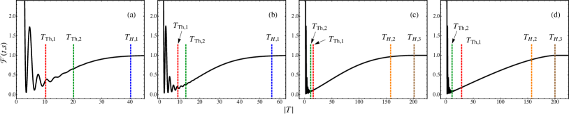
Figure 3: Plots of DSFF and various times for $D=100$, $\varphi=0$ and varying $\tau$: (a) $\tau=0.1$, (b) $\tau=0.7$, (c) $\tau=0.99$, and (d) $\tau=0.9995$. The theoretical estimates for Thouless time ($T_{\mathrm{Th,1}}=(\frac{6}{\pi\eta^{3}(1-\tau^{2})})^{1/5}D^{2/5}$, $T_{\mathrm{Th,2}}=(\frac{3}{2})^{1/4}\frac{D^{1/2}}{\eta}$), and Heisenberg time ($T_{\mathrm{H},1}=4\sqrt{D/(1-\tau^{2})}$, $T_{\mathrm{H},2}=\pi D/(2\eta)$, $T_{\mathrm{H},3}=2D/\eta$) are shown. For (a), (b) in which $\tau\lesssim 1-c/D$; $c=O(1)$, $T_{\mathrm{Th,1}}=$ serves as a better estimate for Thouless time, whereas for (c), (d) for which $\tau\gtrsim 1-c/D$ the value $T_{\mathrm{Th,2}}$ serves better. Similarly, for the Heisenberg time $T_{\mathrm{H,1}}$ serves as a good estimate for (a) and (b). On the other hand, for (c) and (d), $T_{\mathrm{H,2}}$ and $T_{\mathrm{H,3}}$ serve as better estimates, respectively. The $T_{\mathrm{H,1}}$ value in these two panels lie beyond the time scale shown.

For time values in the vicinity of $T_{H}$, the contribution due the connected part becomes small in comparison to the contact part which results in the plateau. Moreover, the disconnected part becomes negligible at a much earlier time. Thus, $T_{H}$ may be estimated using $\mathcal{F}_{\mathrm{conn}}\approx 0$. On expanding Eq. (26) up to $O(1/D)$ and solving for time does lead to $T_{H}=O(\sqrt{D})$ for $\tau=0$ (GinUE), and $T_{H}=O(D)$ for $\tau=1$ (GUE), as is known from earlier works [48, 64]. However, numerical estimate for $T_{H}$ obtained this way does not work well when compared to simulation data for large but finite $D$. The reason is that unless $\tau=1-c/D$, where $c=O(1)$, the exponential term in Eq. (26) leads to a much faster decay of $\mathcal{F}_{\mathrm{conn}}$ towards 0 in comparison to the factor $\mathcal{S}(\sqrt{D\mathcal{T}})$ which remains $O(1)$. To obtain a reasonable estimate for $T_{H}$ in the crossover regime where $\tau<1-c/D$, we may consider $\exp(-\frac{(1-\tau^{2})(t^{2}+s^{2})}{4D})=\exp(\frac{-(1-\tau^{2})|T|^{2}}{4D})=e^{-4}\approx 0.018$ as a convenient choice. This leads to $T_{H}\approx 4\sqrt{D/(1-\tau^{2})}$. For $\tau=1-c/D$, by equating to zero the expansion of $\mathcal{F}_{\mathrm{conn}}$ up to $O(1/D)$, we obtain $T_{H}\approx\pi D/(2\eta)$. This value is less than $2D/\eta$ beyond which $\mathcal{F}_{\mathrm{conn}}$ is identically equal to zero due to the $\mathcal{S}(\sqrt{D\mathscr{T}})$ factor. For $\tau$ closer to 1 than $\tau=1-c/D$, $T_{H}=2D/\eta$ serves as a better and natural estimate.

For time values in the neighborhood of $T_{\mathrm{Th}}$, to extract the leading $|T|$ dependence of the disconnected term $\mathcal{F}_{\mathrm{dis}}$, we can assume $|T|\sim O(D^{\alpha})$, where $0<\alpha<1/2$ and then expand it in $|T|$ considering large $D$. This leads to the $\mathcal{F}_{\mathrm{dis}}$ in this region as $\frac{D}{\pi\eta^{3}|T|^{3}}e^{-\frac{(1-\tau^{2})|T|^{2}}{4D}}\cos^{2}(2\eta|T|+\frac{\pi}{4})\approx\frac{D}{\pi\eta^{3}|T|^{3}}\cos^{2}(2\eta|T|+\frac{\pi}{4})$. Moreover, in this region, the leading behavior of $\mathcal{F}_{\mathrm{conn}}$ is given by $1-\frac{2\eta|T|}{\pi D}-\frac{(1-\tau^{2})|T|^{2}}{4D}$. This expression provides the local behavior of the ramp, which in the GinUE and GUE limits is quadratic and linear, respectively. To obtain an estimate of $T_{\mathrm{Th}}$, we try to locate the minimum of the DSFF using this leading behavior of $\mathcal{F}_{\mathrm{conn}}$ and the nonoscillatory part of $\mathcal{F}_{\mathrm{dis}}$. This results in the quintic equation, $(1-\tau^{2})|T|^{5}+\frac{4\eta}{\pi}|T|^{4}-\frac{6D^{2}}{\pi\eta^{3}}=0$. This predicts $T_{\mathrm{Th}}=O(D^{2/5})$ and $O(D^{1/2})$ for GinUE and GUE, respectively, in agreement with earlier works [48, 63]. In fact, for $\tau\lesssim 1-c/D$, $T_{\mathrm{Th}}\approx(\frac{6}{\pi\eta^{3}(1-\tau^{2})})^{1/5}D^{2/5}$ serves as a very good estimate. On the other hand, for $\tau\gtrsim 1-c/D$, we have $T_{\mathrm{Th}}\approx(\frac{3}{2})^{1/4}\frac{D^{1/2}}{\eta}$. Of course, this approximation breaks down when $\varphi\to\pi/2$, since in this limit $1/\eta\to\infty$. However, towards the GUE limit, one may consider the variable $t=|T|\cos\varphi$ as the effective (real) time variable, which appears in the SFF expression.

In Fig. 3, we test the above estimates for $T_{\mathrm{Th}}$ and $T_{\mathrm{H}}$. We consider $D=100$, $\varphi=0$, and four values of $\tau$. The DSFF curves along with the Thouless and Heisenberg times shown in the plots conform to the assertions made above. We have also tried other parameter values ($D,\varphi$) and found that, depending on considered $\tau$-regime, the proposed estimates for $T_{\mathrm{Th}}$ and $T_{\mathrm{H}}$ work very well.

V Conclusion and Outlook

In this work, we considered the elliptic Ginibre unitary ensemble (eGinUE), a prototypical model for studying Hermiticity breaking in complex systems, and derived exact and asymptotic expressions for the dissipative spectral form factor (DSFF). Furthermore, we unveiled a surprisingly simple relationship between the DSFFs of the eGinUE and the GUE, which enables one to readily obtain the associated results for the former from the latter, which has been studied more extensively. We also provided estimates for the Thouless and Heisenberg times for use in various symmetry regimes between the GinUE and GUE limits. Our findings have been corroborated using Monte Carlo simulations of the eGinUE matrix model. We believe that our results will be immensely useful for examining various spectral traits of non-Hermitian complex systems, where some system parameter may lead to variation in the degree of Hermiticity.

Appendix A Derivation of the DSFF of eGinUE

In this appendix we outline the derivation of the DSFF for eGinUE. It relies on utilizing two important identities involving Hermite polynomials, viz., the addition formula (umbral identity),

$$H_{n}(a+b)=\sum_{l=0}^{n}\binom{n}{l}H_{l}(a)\,(2b)^{n-l},$$ (30)

and the orthogonality relation [65],

$$\int_{-\infty}^{\infty}\int_{-\infty}^{\infty}da\,db\,H_{n}(a+ib)\,H_{m}(a-ib)\,\mathrm{e}^{-ua^{2}-vb^{2}}$$

$$=\frac{\pi}{\sqrt{uv}}\,2^{n}\,n!\,\left(\frac{1}{u}+\frac{1}{v}\right)^{n}\,\delta_{n,m},$$ (31)

where, $\mathrm{Re}(u),\mathrm{Re}(v)>0$. In the disconnected term in Eq. (18), both $z_{1}$ and $z_{2}$ integrals lead to identical result and we need to evaluate

$$\mathcal{F}_{\text{dis}}=\frac{1}{D}\left(\int d^{2}z\,e^{ixt+iys}\,\mathcal{K}(z,z^{*})\right)^{2}.$$ (32)

Equations (13)-(15) are now employed to replace the kernel $\mathcal{K}(z,z^{*})$ within the above integral and gives

$$\mathcal{F}_{\text{dis}}=\frac{1}{D}\left(\sum_{n=0}^{D-1}\frac{D\tau^{n}}{n!\,2^{n}\pi(1-\tau^{2})^{1/2}}I_{n,n}(\tau,t,s)\right)^{2},$$ (33)

where

$$I_{n,m}(\tau,t,s) =\int\,d^{2}zH_{n}\left(\sqrt{\frac{D}{2\tau}}z\right)H_{m}\left(\sqrt{\frac{D}{2\tau}}z^{*}\right)$$

$$\times\exp\Big{(}ixt+iys-\frac{Dx^{2}}{1+\tau}-\frac{Dy^{2}}{1-\tau}\Big{)}.$$ (34)

This evaluation of this integral requires a detailed algebraic calculation aided by Eqs. (30), (A), and yields,

$$\mathcal{F}_{\text{dis}}(t,s) =\frac{e^{-\frac{(1+\tau)t^{2}}{2\,D}-\frac{(1-\tau)s^{2}}{2\,D}}}{D}\left[\sum_{n=0}^{D-1}\sum_{k=0}^{n}\binom{n}{k}\frac{(-\mathscr{T})^{n-k}}{(n-k)!}\right]^{2},$$

where $\mathscr{T}$ is as defined in Eq. (19). The inner sum in this equation is identified as the expansion of Laguerre polynomial $L_{n}(z)\equiv L_{n}^{(0)}(z)$, hence we have,

$$\mathcal{F}_{\text{dis}}(t,s)=\frac{1}{D}e^{-\frac{(1+\tau)t^{2}}{2\,D}-\frac{(1-\tau)s^{2}}{2\,D}}\left[\sum_{n=0}^{D-1}L_{n}^{(0)}(\mathscr{T})\right]^{2}.$$ (36)

Finally, the sum over Laguerre polynomials can be performed using the relation $\sum_{a=0}^{b}L_{a}^{(k)}(z)=L_{b}^{(k+1)}(z)$, which leads to Eq. (18), which is the desired expression.

Next, we aim to evaluate the connected part $\mathcal{F}_{\mathrm{conn}}(t,s)$ and find that

$$\mathcal{F}_{\mathrm{conn}}(t,s)=\frac{1}{D}\int d^{2}z_{1}d^{2}z_{2}\,e^{i\,(x_{1}-x_{2})t+i(y_{1}-y_{2})s}\,|\mathcal{K}(z_{1},z_{2}^{*})|^{2}$$

$$=\frac{D}{\pi^{2}(1-\tau^{2})}\sum_{n,m=0}^{D-1}\frac{(\tau/2)^{n+m}}{n!\,m!}\,I_{n,m}(\tau,t,s)\,I_{n,m}^{*}(\tau,t,s).$$ (37)

Again, a lengthy algebra results in

$$\mathcal{F}_{\text{conn}}(t,s)=\frac{1}{D}e^{-\frac{(1+\tau)t^{2}}{2\,D}-\frac{(1-\tau)s^{2}}{2\,D}}\sum_{n,m=0}^{D-1}\frac{(4\,D)^{-(n+m)}}{n!\,m!}$$

$$\times\left|\sum_{k=0}^{\min(n,m)}\binom{n}{k}\binom{m}{k}\frac{k!}{(4\,D)^{-k}}\frac{\left[i(1+\tau)t-(1-\tau)s\right]^{n-k}}{\left[i(1+\tau)t+(1-\tau)s\right]^{k-m}}\right|^{2}.$$ (38)

Mathematica [66] is able to perform the inner double-sum in terms of Tricomi confluent hypergeometric function, which can be equivalently written in terms of associated Laguerre polynomial, as done in Eq. (IV).

Appendix B Derivation of large-$D$ DSFF results

For the disconnected part, Eq. (18), we use the following result for the associated Laguerre polynomials which holds for large $D$, but fixed $\alpha$ and $x>0$ [67]:

$$L_{D}^{(\alpha)}(x/D)=D^{\alpha}x^{-\alpha/2}J_{\alpha}(2x^{1/2}),$$ (39)

where, as indicated earlier, $J_{\alpha}(u)$ is the Bessel function of order $\alpha$. This readily leads to the large-$D$ approximation given in Eq. (25). The connected part of the DSFF is more involved due to presence of double sum, as given in Eq. (IV). Fortunately, for the connected part, a very good approximation for the SFF (equivalently DSFF) of GUE has been derived in Ref. [64], which is given by

$$\mathcal{F}^{\mathrm{GUE}}_{\mathrm{conn}}(t)\approx\mathcal{S}(t),$$ (40)

where $\mathcal{S}(t)$ is defined in Eq. (27). Based on this result and the scaling relation, Eq. (24), we can at once write down the large $D$ approximation for the connected part of the eGinUE DSFF, as is given in Eq. (26). In the $\tau=0$ and $\tau=1$ limits, we readily obtain the large $D$ approximation for DSFF of GinUE and GUE as presented in Eqs. (IV) and (29).

References

- Berry [1985] M. V. Berry, Semiclassical theory of spectral rigidity, Proc. R. Soc. Lond. A 400, 229 (1985).
- Leviandier et al. [1986] L. Leviandier, M. Lombardi, R. Jost, and J. P. Pique, Fourier transform: A tool to measure statistical level properties in very complex spectra, Phys. Rev. Lett. 56, 2449 (1986).
- Brézin and Hikami [1997] E. Brézin and S. Hikami, Spectral form factor in a random matrix theory, Phys. Rev. E 55, 4067 (1997).
- Gharibyan et al. [2018] H. Gharibyan, M. Hanada, S. H. Shenker, and M. Tezuka, Onset of random matrix behavior in scrambling systems, J. High Energy Phys. 2018, 1 (2018).
- Saad et al. [2018] P. Saad, S. H. Shenker, and D. Stanford, A semiclassical ramp in SYK and in gravity, arXiv:1806.06840 (2018).
- Gaikwad and Sinha [2019] A. Gaikwad and R. Sinha, Spectral form factor in non-Gaussian random matrix theories, Phys. Rev. D 100, 026017 (2019).
- Winer et al. [2020] M. Winer, S. K. Jian, and B. Swingle, Exponential Ramp in the Quadratic Sachdev-Ye-Kitaev Model, Phys. Rev. Lett. 125, 250602 (2020).
- Forrester [2021] P. J. Forrester, Quantifying dip–ramp–plateau for the Laguerre unitary ensemble structure function, Commun. Math. Phys. 387, 215 (2021).
- Schiulaz, Mauro and Torres-Herrera, E Jonathan and Santos, Lea F [2019] Schiulaz, Mauro and Torres-Herrera, E Jonathan and Santos, Lea F, Thouless and relaxation time scales in many-body quantum systems, Phys. Rev. B 99, 174313 (2019).
- Lezama, Talía LM and Torres-Herrera, E Jonathan and Pérez-Bernal, Francisco and Bar Lev, Yevgeny and Santos, Lea F [2021] Lezama, Talía LM and Torres-Herrera, E Jonathan and Pérez-Bernal, Francisco and Bar Lev, Yevgeny and Santos, Lea F, Equilibration time in many-body quantum systems, Phys. Rev. B 104, 085117 (2021).
- Tameshtit and Sipe [1992] A. Tameshtit and J. E. Sipe, Survival probability and chaos in an open quantum system, Phys. Rev. A 45, 8280 (1992).
- Xu et al. [2021] Z. Xu, A. Chenu, T. Prosen, and A. del Campo, Thermofield dynamics: Quantum chaos versus decoherence, Phys. Rev. B 103, 064309 (2021).
- Cornelius et al. [2022] J. Cornelius, Z. Xu, A. Saxena, A. Chenu, and A. del Campo, Spectral Filtering Induced by Non-Hermitian Evolution with Balanced Gain and Loss: Enhancing Quantum Chaos, Phys. Rev. Lett. 128, 190402 (2022).
- Matsoukas-Roubeas, Apollonas S and Roccati, Federico and Cornelius, Julien and Xu, Zhenyu and Chenu, Aurélia and del Campo, Adolfo [2023] Matsoukas-Roubeas, Apollonas S and Roccati, Federico and Cornelius, Julien and Xu, Zhenyu and Chenu, Aurélia and del Campo, Adolfo, Non-Hermitian Hamiltonian deformations in quantum mechanics, J. High Energy Phys. 2023, 1 (2023).
- Matsoukas-Roubeas et al. [2023] A. S. Matsoukas-Roubeas, M. Beau, L. F. Santos, and A. del Campo, Unitarity breaking in self-averaging spectral form factors, Phys. Rev. A 108, 062201 (2023).
- Vasilyev et al. [2020] D. V. Vasilyev, A. Grankin, M. A. Baranov, L. M. Sieberer, and P. Zoller, Monitoring Quantum Simulators via Quantum Nondemolition Couplings to Atomic Clock Qubits, PRX Quantum 1, 020302 (2020).
- Nivedita et al. [2020] Nivedita, H. Shackleton, and S. Sachdev, Spectral form factors of clean and random quantum Ising chains, Phys. Rev. E 101, 042136 (2020).
- Šuntajs et al. [2020] J. Šuntajs, J. Bonča, T. Prosen, and L. Vidmar, Quantum chaos challenges many-body localization, Phys. Rev. E 102, 062144 (2020).
- Prakash et al. [2021] A. Prakash, J. Pixley, and M. Kulkarni, Universal spectral form factor for many-body localization, Phys.l Rev. Res. 3, L012019 (2021).
- Sarkar et al. [2024] A. Sarkar, S. Pachhal, A. Agarwala, and D. Das, Spectral form factors of topological phases, Phys. Rev. B 109, 155126 (2024).
- Grobe et al. [1988] R. Grobe, F. Haake, and H. J. Sommers, Quantum Distinction of Regular and Chaotic Dissipative Motion, Phys. Rev. Lett. 61, 1899 (1988).
- Chalker and Wang [1997] J. T. Chalker and Z. J. Wang, Diffusion in a Random Velocity Field: Spectral Properties of a Non-Hermitian Fokker-Planck Operator, Phys. Rev. Lett. 79, 1797 (1997).
- Müller et al. [2012] M. Müller, S. Diehl, G. Pupillo, and P. Zoller, Engineered open systems and quantum simulations with atoms and ions, in Advances in Atomic, Molecular, and Optical Physics, Vol. 61 (Elsevier, 2012) pp. 1–80.
- Can [2019] T. Can, Random lindblad dynamics, J. Phys. A Math. Theor. 52, 485302 (2019).
- Sá et al. [2020] L. Sá, P. Ribeiro, and T. Prosen, Spectral and steady-state properties of random Liouvillians, J. Phys. A Math. Theor. 53, 305303 (2020).
- Makris et al. [2008] K. G. Makris, R. El-Ganainy, D. N. Christodoulides, and Z. H. Musslimani, Beam Dynamics in Symmetric Optical Lattices, Phys. Rev. Lett. 100, 103904 (2008).
- Klaiman et al. [2008] S. Klaiman, U. Günther, and N. Moiseyev, Visualization of Branch Points in -Symmetric Waveguides, Phys. Rev. Lett. 101, 080402 (2008).
- Rüter et al. [2010] C. E. Rüter, K. G. Makris, R. El-Ganainy, D. N. Christodoulides, M. Segev, and D. Kip, Observation of parity–time symmetry in optics, Nat. Phys. 6, 192 (2010).
- Konotop et al. [2016] V. V. Konotop, J. Yang, and D. A. Zezyulin, Nonlinear waves in -symmetric systems, Rev. Mod. Phys. 88, 035002 (2016).
- Feng et al. [2017] L. Feng, R. El-Ganainy, and L. Ge, Non-Hermitian photonics based on parity–time symmetry, Nat. Photon. 11, 752 (2017).
- El-Ganainy et al. [2018] R. El-Ganainy, K. G. Makris, M. Khajavikhan, Z. H. Musslimani, S. Rotter, and D. N. Christodoulides, Non-Hermitian physics and PT symmetry, Nat. Phys. 14, 11 (2018).
- Gupta et al. [2020] S. K. Gupta, Y. Zou, X. Y. Zhu, M. H. Lu, L. J. Zhang, X. P. Liu, and Y. F. Chen, Parity-time symmetry in non-Hermitian complex optical media, Adv. Mater. 32, 1903639 (2020).
- Tzortzakakis et al. [2020] A. F. Tzortzakakis, K. G. Makris, and E. N. Economou, Non-Hermitian disorder in two-dimensional optical lattices, Phys. Rev. B 101, 014202 (2020).
- Zhang et al. [2022] S. B. Zhang, M. M. Denner, T. Bzdušek, M. A. Sentef, and T. Neupert, Symmetry breaking and spectral structure of the interacting Hatano-Nelson model, Phys. Rev. B 106, L121102 (2022).
- Ghatak et al. [2020] A. Ghatak, M. Brandenbourger, J. Van Wezel, and C. Coulais, Observation of non-Hermitian topology and its bulk–edge correspondence in an active mechanical metamaterial, Proceedings of the National Academy of Sciences 117, 29561 (2020).
- Kawabata et al. [2018a] K. Kawabata, K. Shiozaki, and M. Ueda, Anomalous helical edge states in a non-Hermitian Chern insulator, Phys. Rev. B 98, 165148 (2018a).
- Kawabata et al. [2018b] K. Kawabata, Y. Ashida, H. Katsura, and M. Ueda, Parity-time-symmetric topological superconductor, Phys. Rev. B 98, 085116 (2018b).
- Yao et al. [2018] S. Yao, F. Song, and Z. Wang, Non-Hermitian Chern Bands, Phys. Rev. Lett. 121, 136802 (2018).
- Ginibre [1965] J. Ginibre, Statistical ensembles of complex, quaternion, and real matrices, J. Math. Phys. 6, 440 (1965).
- Sommers et al. [1988] H. J. Sommers, A. Crisanti, H. Sompolinsky, and Y. Stein, Spectrum of Large Random Asymmetric Matrices, Phys. Rev. Lett. 60, 1895 (1988).
- Lehmann and Sommers [1991] N. Lehmann and H. J. Sommers, Eigenvalue statistics of random real matrices, Phys. Rev. Lett. 67, 941 (1991).
- Hamazaki et al. [2019] R. Hamazaki, K. Kawabata, and M. Ueda, Non-Hermitian Many-Body Localization, Phys. Rev. Lett. 123, 090603 (2019).
- Akemann et al. [2019] G. Akemann, M. Kieburg, A. Mielke, and T. Prosen, Universal Signature from Integrability to Chaos in Dissipative Open Quantum Systems, Phys. Rev. Lett. 123, 254101 (2019).
- Sá et al. [2020] L. Sá, P. Ribeiro, and T. Prosen, Complex Spacing Ratios: A Signature of Dissipative Quantum Chaos, Phys. Rev. X 10, 021019 (2020).
- Ghosh et al. [2022] S. Ghosh, S. Gupta, and M. Kulkarni, Spectral properties of disordered interacting non-Hermitian systems, Phys. Rev. B 106, 134202 (2022).
- Shivam et al. [2023] S. Shivam, A. De Luca, D. A. Huse, and A. Chan, Many-body quantum chaos and emergence of Ginibre ensemble, Phys. Rev. Lett. 130, 140403 (2023).
- Kawabata et al. [2023] K. Kawabata, A. Kulkarni, J. Li, T. Numasawa, and S. Ryu, Dynamical quantum phase transitions in Sachdev-Ye-Kitaev lindbladians, Phys. Rev. B 108, 075110 (2023).
- Li et al. [2021] J. Li, T. Prosen, and A. Chan, Spectral Statistics of Non-Hermitian Matrices and Dissipative Quantum Chaos, Phys. Rev. Lett. 127, 170602 (2021).
- García-García et al. [2023] A. M. García-García, L. Sá, and J. J. Verbaarschot, Universality and its limits in non-Hermitian many-body quantum chaos using the Sachdev-Ye-Kitaev model, Phys. Rev. D 107, 066007 (2023).
- Akemann and Vernizzi [2003] G. Akemann and G. Vernizzi, Characteristic polynomials of complex random matrix models, Nucl. Phys. B 660, 532 (2003).
- Khoruzhenko and Sommers [2015] B. Khoruzhenko and H. J. Sommers, Non-Hermitian ensembles, in The Oxford Handbook of Random Matrix Theory (Oxford University Press, 2015).
- Forrester [2010] P. J. Forrester, Log-gases and random matrices (LMS-34) (Princeton University Press, 2010).
- Mehta [2004] M. L. Mehta, Random matrices (Elsevier, 2004).
- Fyodorov et al. [1997a] Y. V. Fyodorov, B. A. Khoruzhenko, and H. J. Sommers, Almost Hermitian random matrices: crossover from Wigner-Dyson to Ginibre eigenvalue statistics, Phys. Rev. Lett. 79, 557 (1997a).
- Fyodorov et al. [1997b] Y. V. Fyodorov, B. A. Khoruzhenko, and H. J. Sommers, Almost-Hermitian random matrices: eigenvalue density in the complex plane, Phys. Lett. A 226, 46 (1997b).
- Fyodorov et al. [1998] Y. V. Fyodorov, H. J. Sommers, and B. A. Khoruzhenko, Universality in the random matrix spectra in the regime of weak non-Hermiticity, in Annales de l’IHP Physique théorique, Vol. 68 (1998) pp. 449–489.
- Dyer and Gur-Ari [2017] E. Dyer and G. Gur-Ari, 2D CFT partition functions at late times, J. High Energy Phys. 2017, 1 (2017).
- del Campo et al. [2018] A. del Campo, J. Molina Vilaplana, L. F. Santos, and J. Sonner, Decay of a thermofield-double state in chaotic quantum systems: From random matrices to spin systems, Eur. Phys. J.: Spec. Top. 227, 247 (2018).
- Forrester and Jancovici [1996] P. J. Forrester and B. Jancovici, Two-dimensional one-component plasma in a quadrupolar field, Int. J. Mod. Phys. A 11, 941 (1996).
- Akemann et al. [2023] G. Akemann, M. Duits, and L. Molag, The elliptic Ginibre ensemble: A unifying approach to local and global statistics for higher dimensions, J. Math. Phys. 64 (2023).
- Girko [1986] V. L. Girko, Elliptic law, Theory Probab. Appl. 30, 677 (1986).
- Di Francesco et al. [1994] P. Di Francesco, M. Gaudin, C. Itzykson, and F. Lesage, Laughlin’s wave functions, Coulomb gases and expansions of the discriminant, Int. J. Mod. Phys. A 9, 4257 (1994).
- Del Campo et al. [2017] A. Del Campo, J. Molina Vilaplana, and J. Sonner, Scrambling the spectral form factor: unitarity constraints and exact results, Phys. Rev. D 95, 126008 (2017).
- Liu [2018] J. Liu, Spectral form factors and late time quantum chaos, Phys. Rev. D 98, 086026 (2018).
- Van Eijndhoven and Meyers [1990] S. Van Eijndhoven and J. Meyers, New orthogonality relations for the Hermite polynomials and related Hilbert spaces, J. Math. Anal. Appl. 146, 89 (1990).
- [66] Wolfram Research, Inc., Mathematica, Version 13.3, (Wolfram Research, Inc., Champaign, IL, 2023).
- Szeg [1939] G. Szeg, Orthogonal polynomials, Vol. 23 (American Mathematical Soc., 1939) p. 193.