Parameter-Efficient Fine-Tuning for Continual Learning: A Neural Tangent Kernel Perspective

Abstract

Parameter-efficient fine-tuning for continual learning (PEFT-CL) has shown promise in adapting pre-trained models to sequential tasks while mitigating catastrophic forgetting problem. However, understanding the mechanisms that dictate continual performance in this paradigm remains elusive. To tackle this complexity, we undertake a rigorous analysis of PEFT-CL dynamics to derive relevant metrics for continual scenarios using Neural Tangent Kernel (NTK) theory. With the aid of NTK as a mathematical analysis tool, we recast the challenge of test-time forgetting into the quantifiable generalization gaps during training, identifying three key factors that influence these gaps and the performance of PEFT-CL: training sample size, task-level feature orthogonality, and regularization. To address these challenges, we introduce NTK-CL, a novel framework that eliminates task-specific parameter storage while adaptively generating task-relevant features. Aligning with theoretical guidance, NTK-CL triples the feature representation of each sample, theoretically and empirically reducing the magnitude of both task-interplay and task-specific generalization gaps. Grounded in NTK analysis, our approach imposes an adaptive exponential moving average mechanism and constraints on task-level feature orthogonality, maintaining intra-task NTK forms while attenuating inter-task NTK forms. Ultimately, by fine-tuning optimizable parameters with appropriate regularization, NTK-CL achieves state-of-the-art performance on established PEFT-CL benchmarks. This work provides a theoretical foundation for understanding and improving PEFT-CL models, offering insights into the interplay between feature representation, task orthogonality, and generalization, contributing to the development of more efficient continual learning systems.

1 Introduction

In practical applications, the relentless evolution of environments underscores the urgency for learning systems that can progressively accumulate knowledge. This has led to the prominence of Continual Learning (CL) [54, 87, 13, 60, 43, 78, 53], a cornerstone task that equips the learning models with the ability to seamlessly assimilate fresh information over time, while mitigating catastrophic forgetting, i.e., a phenomenon that erodes previously acquired knowledge. In recent years, with the proliferation of pre-trained models possessing strong generalization capabilities [6, 63], researchers have discovered that they can empower early exploratory methods [7, 80, 18, 22, 52, 4, 68, 97, 69, 90, 89, 99, 44, 46, 45, 33, 88], enabling CL systems to integrate new knowledge more efficiently. However, full fine-tuning of pre-trained models is computationally intensive and may compromise their original generalization capabilities [27, 50, 94]. Thus, as a promising paradigm, Parameter-Efficient Fine-Tuning for Continual Learning (PEFT-CL) emerges as an alternative, updating only a minimal set of additional parameters while keeping the pre-trained model intact. Specifically, PEFT-CL not only offers a more philosophically sound framework akin to Socratic dialogue [95] but also provides a lightweight training process that avoids generalization deterioration associated with full-scale fine-tuning [35, 76]. In addition, this seamless integration of new and old knowledge aligns with the wisdom expressed by Bernard of Chartres, demonstrating how PEFT-CL builds upon pre-existing knowledge to achieve a more adaptive learner with robust memory capabilities.

Despite initial successes in mitigating catastrophic forgetting [82, 81, 71, 19, 100], PEFT-CL largely relies on subjective human insights and experiential doctrines for network design and enhancement, lacking a rigorous mathematical foundation. This reliance on non-theoretical approaches constrains the potential for a deeper understanding and advancement of the fundamental mechanisms within these learning systems. While Hide-Prompt [77] acknowledges the importance of addressing this issue and offers a loss-based perspective, it falls short of modeling optimization dynamics and pinpointing key factors. Therefore, to address this gap, we adopt the Neural Tangent Kernel (NTK) theory [32, 8, 5] as a robust mathematical tool to delve deeply into the intricacies of PEFT-CL optimization. Through this rigorous analysis, we derive several fundamental theorems and lemmas, including theorem 1, theorem 2, lemma 3, and theorem 4. While initially considered from a CL perspective, these have been generalized to the PEFT-CL scenario, providing profound insights into the key factors essential for effectively combating catastrophic forgetting in PEFT-CL optimization. Guided by these theories and key factors, we develop an NTK-CL framework, effectively reducing the quantified catastrophic forgetting discussed later.

In addition to theoretical advantages, we also detail the differences in structure and optimization between our NTK-CL framework and current mainstream methodologies in Fig. 1. Unlike the Additional Subnetworks paradigm (Fig. 1a), which constructs task-specific subnetwork parameter spaces and concatenates features from all network parameter spaces at inference time [100, 19, 48], or the Prompts Optimization paradigm (Fig. 1b), which builds task-specific prompt pools for input interaction and employs cosine similarity for prompt selection [82, 36, 81, 71, 62], NTK-CL (Fig. 1c) eliminates the need for task-specific parameter storage or prompt pools. Instead, it leverages a shared network parameter space across all tasks to adaptively generate task-relevant features based on input characteristics. Specifically, its design and optimization are entirely derived from NTK-based generalization gaps, which not only triple the expansion of sample representations but also consider knowledge retention, task-feature dissimilarity, and regularization term.

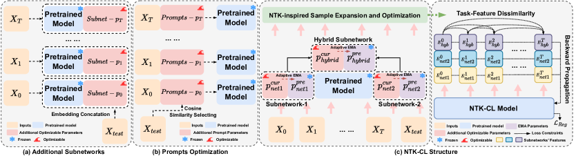
Figure 1: Comparison chart between the mainstream frameworks in PEFT-CL and our NTK-CL framework.

Overall, our contributions are delineated across three primary areas:

• Theoretical Exploration of PEFT-CL: We pioneer the analysis of PEFT-CL through NTK lens and foundational mathematics. Through a series of derived theorems and lemmas, we identify critical factors that optimize PEFT-CL learners, including the number of samples in data subsets, the total sample volume across the dataset, knowledge retention strategies, task-feature dissimilarity constraints, and adjustments to regularization terms.

• Innovative Solutions Based on Key Factors: Leveraging theoretical insights, we propose an NTK-CL framework, incorporating multiple interventions to expand each sample’s representational breadth, an adaptive Exponential Moving Average (EMA) mechanism that preserves intra-task NTK forms (enhancing knowledge retention), task-feature orthogonality constraints that attenuate inter-task NTK forms (increasing knowledge separability), and tailored regularization adjustments that meet the theoretical prerequisites for solving PEFT-CL dynamics. With these strategies, we optimally minimize the generalization gaps and population losses in both task-interplay and task-specific settings for PEFT-CL scenario, significantly mitigating the catastrophic forgetting problem both theoretically and practically.

• Empirical Validation on Diverse Datasets: We conduct extensive experiments across various datasets to validate the effectiveness of our key factors and methodologies. Additionally, we perform fair comparisons against numerous state-of-the-art methods, ensuring consistent task segmentations to mitigate performance discrepancies. This comprehensive validation substantiates the efficacy of our theoretical innovations in practical applications.

These contributions significantly advance PEFT-CL field, bridging the gap between theoretical foundations and practical efficacy in enhancing model performance and generalization across diverse learning environments.

2 Related Works

Parameter-Efficient Fine-Tuning has emerged as a pivotal paradigm for optimizing model performance while mitigating computational and memory burdens associated with large-scale model adaptation. Seminal works introduce diverse methodologies, including Adapter modules [26], Low-Rank Adaptation (LoRA) [27], Prefix Tuning [47], Prompt Tuning [6], and BitFit [96]. These approaches demonstrate the efficacy of selectively fine-tuning components or introducing compact, trainable sub-networks within pre-trained architectures. Subsequent advancements further expand PEFT’s scope and capabilities. Jia et al. [34] pioneer efficient prompt tuning techniques for vision transformers, extending PEFT’s applicability to the visual domain. Zhou et al. [102] introduce contextual prompt fine-tuning, enhancing model adaptability while preserving generalization. Recent comprehensive studies [20, 85, 86, 15] reinforce PEFT’s critical role in enhancing model generalization and efficiency. These investigations rigorously analyze the theoretical underpinnings and empirical efficacy of various PEFT methodologies, solidifying its status as a transformative paradigm in adaptive learning.

Continual Learning is a critical field in artificial intelligence aimed at developing models that can learn new tasks while preserving knowledge from previous tasks. This field encompasses both task-specific strategies and generalization-based approaches. Task-specific strategies utilize four primary methodologies to address continual learning challenges: replay-based, parameter regularization, dynamic networks, and knowledge distillation. Replay-based methods [7, 80, 18, 22] mitigate catastrophic forgetting through selective sample storage and data generation. Regularization-based approaches [52, 4, 68, 97] limit alterations to crucial parameters, integrating various regularization methods to stabilize performance across tasks. Architecture-based strategies [69, 90, 89, 99] modify network structures to accommodate new information, employing dynamically expanding ensembles and structural adjustments based on task relevance. Distillation-based techniques [44, 46, 45, 33, 88] leverage knowledge transfer to maintain continuity of information across tasks. Generalization-based methods focus on model generalization that inherently support knowledge transfer and retention across tasks. [49] delves into balancing retention with generalization, while [64] provides insights into the interplay between learning new information and retaining old knowledge. [65] examines the role of controlled forgetting in enhancing model resilience, and [1] assesses the implications of network reinitialization on learning dynamics and generalization. Similar foundational investigations by [84, 37, 3, 16] explore continual learning through the lenses of NTK and generalization theory, though these studies primarily address traditional continual learning scenarios and do not fully integrate advancements from the era of pre-trained models.

Parameter-Efficient Fine-Tuning for Continual Learning has established itself as an effective strategy to to counter catastrophic forgetting by training minimal additional parameters atop pre-trained models. Notable approaches such as L2P [82] and DualPrompt [81] introduce task-specific and dual prompts, respectively, facilitating adaptive task-specific learning while preserving invariant knowledge. S-Prompt [79] employs structural prompts to map discriminative domain relationships, while CODA-Prompt [71] applies Schmidt orthogonalization to refine these prompts. Concurrently, DAP [36] innovates by constructing real-time instance-level dynamic sub-networks to adapt to various domains. Moreover, HiDe-Prompt [77] integrates task-level knowledge sub-networks with distributional statistics to sample past data, thereby preventing suboptimal learning trajectories. EASE [100] further contributes by optimizing task-specific and expandable adapters to enhance knowledge retention. Despite these advancements, the reliance on specific configurations underscores the necessity for deeper theoretical exploration to fundamentally address PEFT-CL’s challenges, necessitating a shift towards a NTK perspective to enrich our understanding and efficacy in PEFT-CL.

3 Preliminaries

In the PEFT-CL context, we augment pre-trained models with adaptive sub-networks to manage sequential tasks. Let $f^{*}_{0}$ and $f^{*}_{T}$ denote the initial and target parameter spaces respectively, with $*$ indicating optimized parameters. Given a series of tasks $\mathcal{D}=\{\mathcal{D}_{1},\ldots,\mathcal{D}_{T}\}$, where each $\mathcal{D}_{\tau}$ comprises samples $(x,y)$ from $(X_{\tau},Y_{\tau})$, we introduce task-specific optimizable sub-network parameters $p_{\tau}$. The transformed model is represented as $f^{*}_{\tau}=(f^{*}_{0}\circ p_{\tau}\circ X_{\tau}\circ Y_{\tau})$, with $\circ$ denoting component integration. This configuration, inspired by L2P [82], features distinct class boundaries without explicit task identification during training, aligning with practical scenarios.

Empirical NTK: The NTK elucidates infinite-width neural network training dynamics, mapping the learning trajectory in high-dimensional parameter space [32]. Leveraging NTK’s spectral properties enables precise predictions about network generalization, linking architectural choices to extrapolation performance [5]. However, practical NTK calculation faces challenges due to extensive gradient computations across entire datasets. The empirical NTK [32] addresses this, providing a more tractable analytical tool:

$$\Phi_{p_{\tau}}(x_{1},x_{2})=\left[J_{p_{\tau}}(f_{p_{\tau}}(x_{1}))\right]\left[J_{p_{\tau}}(f_{p_{\tau}}(x_{2}))\right]^{\top},$$ (1)

where $J_{p_{\tau}}(f_{p_{\tau}}(x))$ denotes the Jacobian matrix of network $f_{\tau}$ with parameters optimized for task $\tau$, evaluated at input $x$. This function maps $D$-dimensional inputs to $O$-dimensional features, with $J_{p_{\tau}}(f_{p_{\tau}}(x))\in\mathbb{R}^{O\times P}$ and $\Phi_{p_{\tau}}(x_{1},x_{2})\in\mathbb{R}^{O\times O}$.

Neural Tangent Kernel Regime: As layer widths approach infinity, the NTK characterizes the asymptotic behavior of neural networks, yielding a time-invariant NTK throughout training [32, 42]. This induces a linear dynamical system in function space, governed by the following evolution equation for the output $f(x,\theta)$ at input $x$:

$$\frac{\partial f(x,\theta(t))}{\partial t}=-\Phi(x,X)\nabla_{f}\mathcal{L}(f(X,\theta(t)),Y)$$ (2)

where $\Phi(x,X)$ denotes the NTK matrix, $X$ represents the entire training dataset, $Y$ corresponds to labels, and $\mathcal{L}$ signifies the loss function.

This formulation elucidates the network’s trajectory towards the global minimum, exhibiting exponential convergence under a positive definite NTK [32, 42, 56, 8, 5, 92]. Furthermore, in PEFT-CL, to better adapt it for sequence learning scenarios, we have transformed it in Appendix A as follows:

$$f_{T}(x)= f_{0}^{*}(x)+\sum\limits_{i=1}^{T}\Phi_{i}(x,X)$$ (3)

$$\times(\Phi_{i}(X,X)+\lambda I)^{-1}(Y_{i}-f_{i-1}^{*}(X)),$$

where $\Phi_{i}$ represents the locally converged NTK matrix for the $i$-th task.

Remark: The NTK paradigm is effective across various neural architectures, including ResNets and Transformers [92, 93], with primary variations evident in the configuration of the NTK matrix. Ideally, all $\Phi_{i}$ matrices would evolve towards a consistent $\Phi$ as the model trains [32, 8].

4 Theoretical Insights

The prevalent belief in PEFT-CL methods is that mitigating catastrophic forgetting should be evaluated based on accuracy, specifically by calculating the difference between the optimal accuracy on a previous task during its optimization and the accuracy on that task at the final stage. However, using abstract accuracy metrics is not conducive to precise mathematical quantification, and the accuracy gap during testing cannot effectively intervene in training. To better align with the role of NTK in studying model generalization, we propose shifting the focus from the accuracy gap to the generalization gap. This shift allows for rigorous mathematical analysis related to training conditions and aligns with established principles of generalizability [103, 51].

Harnessing the interpretative power of the NTK to decode network training dynamics, we assess the model’s resilience against forgetting through the generalization gaps and population losses. Initially, we derive the general formulation of cross-task generalization gap and population loss for the PEFT-CL scenario, addressing data from the $\tau$-th task post the final training session. We further extend our analysis, which assesses the population loss for individual tasks using NTK spectral theory. By examining the commonalities in these losses, we identify key elements that influence the optimization process of the PEFT-CL model and propose further theoretical insights. These concepts will be elaborated upon in a step-by-step manner. .

Theorem 1 (Task-Interplay Generalization in PEFT-CL).

Consider a sequence of kernel functions $\{\Phi_{\tau}:\mathcal{X}\times\mathcal{X}\rightarrow\mathbb{R}\}_{\tau=1}^{T}$ and corresponding feature maps $\varphi_{\tau}:\mathcal{X}\rightarrow\mathcal{H}$, where $\mathcal{H}$ represents a Hilbert space. For any function $f$ within $\mathcal{F}_{T}$, it is established with at least $1-\delta$ confidence that the discrepancy between the population loss $L_{D}(f(X_{\tau}))$ and the empirical loss $L_{S}(f(X_{\tau}))$ for the $\tau$-th task’s data is bounded by:

$$\footnotesize\sup_{f\in\mathcal{F}_{T}}\{L_{D}(f(X_{\tau}))-L_{S}(f(X_{\tau}))\}\leq 2\rho\hat{\mathcal{R}}(\mathcal{F}_{T})+3c\sqrt{\frac{\log(2/\delta)}{2N}},$$ (4)

where $\rho$ denotes the Lipschitz constant, $c$ a constant, and $N$ the total sample count.

Moreover, if $f^{*}_{T}$ is the optimally selected function from $\mathcal{F}_{T}$, the upper bound for the population loss $L_{D}(f^{*}_{T})$ in relation to the empirical loss $L_{S}(f^{*}_{T})$ can be expressed as:

$$\small L_{D}(f^{*}_{T}(X_{\tau}))\leq L_{S}(f^{*}_{T}(X_{\tau}))+2\rho\hat{\mathcal{R}}(\mathcal{F}_{T})+3c\sqrt{\frac{\log(2/\delta)}{2N}},$$ (5)

$$\footnotesize\begin{split}\mathcal{L}_{S}(f_{T}^{*}(X_{\tau}))\leq&\frac{1}{n_{\tau}}\bigg{[}\lambda^{2}\tilde{Y}_{\tau}^{\top}(\Phi_{\tau}(X_{\tau},X_{\tau})+\lambda I)^{-1}\tilde{Y}_{\tau}+\sum_{k=\tau+1}^{T}\tilde{Y}_{k}^{\top}\\ &\times(\Phi_{k}(X_{k},X_{k})+\lambda I)^{-1}\Phi_{k}(X_{\tau},X_{k})\\ &\times\Phi_{k}(X_{\tau},X_{k})^{\top}(\Phi_{k}(X_{k},X_{k})+\lambda I)^{-1}\tilde{Y}_{k}\bigg{]}_{\mathcal{D}_{\tau}},\end{split}$$ (6)

$$\small\hat{\mathcal{R}}(\mathcal{F}_{T})\leq\left[\sum\limits_{\tau=1}^{T}\mathcal{O}(\sqrt{\frac{[\tilde{Y}_{\tau}^{\top}(\Phi_{\tau}(X,X)+\lambda I)^{-1}\tilde{Y}_{\tau}]}{n_{\tau}}})\right]_{\mathcal{D}_{\tau}}.$$ (7)

Theorem 2 (Task-Specific Generalization in PEFT-CL).

In the realm of PEFT-CL, consider a sequence of learning tasks, each uniquely identified by an index $\tau$. For each task $\tau$, define $f^{*}_{\tau}(x)$ as the task-specific optimal function, whose performance is critically influenced by the spectral properties of the NTK. The population loss, $L_{D}(f^{*}_{\tau})$, for task $\tau$ is influenced by these spectral properties, and can be quantified as follows:

$$\small L_{D}(f^{*}_{\tau})=\sum\limits_{\rho,i}\frac{w_{\rho}^{*2}}{\lambda_{\rho}}\left(\frac{1}{\lambda_{\rho}}+\frac{s_{i}}{\lambda+tu_{i}}\right)^{-2}(1-\frac{m_{i}s_{i}}{(\lambda+tu_{i})^{2}})^{-1},$$ (8)

Here, $\rho$ indexes the eigenvalues, $\lambda_{\rho}$ and $w_{\rho}^{*}$ are the eigenvalues and the optimal weights associated with the orthogonal basis functions of the kernel, respectively. The variable $s_{i}$ indicates the sample size for $i=1,2,\ldots,n_{\tau}$. The parameters $m_{i}$ and $tu_{i}$ are derived from the established relationships:

$$\small m_{i}=\sum_{\rho,i}(\frac{1}{\lambda_{\rho}}+\frac{s_{i}}{\lambda+m_{i}})^{-1},\quad tu_{i}=\sum_{\rho,i}(\frac{1}{\lambda_{\rho}}+\frac{s_{i}}{\lambda+m_{i}})^{-2}.$$ (9)

To clarify the exposition, we detail the derivation processes for theorem 1 and theorem 2 in Appendix B and Appendix C, respectively. Building on these foundations, we further analyze and derive lemma 3, establishing the basis for the details of subsequent NTK-CL implementations.

Lemma 3 (Enhanced Generalization in PEFT-CL).

Within the PEFT-CL scenario, targeted optimizations are essential for augmenting generalization across tasks and bolstering knowledge transfer. Based on the insights from theorem 1 and theorem 2, the following pivotal strategies are identified to enhance generalization:

1. Sample Size Expansion: Increasing both $n_{\tau}$ and $N$ effectively reduces the empirical loss and Rademacher complexity, which in turn lowers the generalization gap and the population loss $L_{D}(f^{*}_{\tau})$.

2. Task-Level Feature Constraints: Preserving the original past knowledge and intensifying inter-task feature dissimilarity, i.e., by maintaining $\Phi_{\tau}(X_{\tau},X_{\tau})$ and $\Phi_{k}(X_{k},X_{k})$, while minimizing $\Phi_{k}(X_{\tau},X_{k})$, adheres to the theoretical underpinnings posited in [16].

3. Regularization Adjustment: Fine-tuning the regularization parameter $\lambda$ helps optimize the model complexity and the empirical loss, mitigating catastrophic forgetting problem. In addition, adjusting $\lambda$ influences the eigenvalue distribution within the NTK framework, directly affecting the kernel’s conditioning and the generalization bounds as established for $f^{*}_{\tau}(x)$.

Proof Outline: The lemma unfolds through an analysis of the interrelations among Rademacher complexity , empirical loss, and NTK spectral characteristics, as discussed in theorem 1 and theorem 2. It underscores the significance of sample size expansion, the delineation of task-level features as instrumental, and meticulous regularization to advancing generalization and fostering knowledge retention within PEFT-CL environments.

From lemma 3, we identify the key factors that need attention during the optimization process of the PEFT-CL model and further propose the NTK-CL framework, planned from the NTK perspective, based on these focal points.

5 NTK-CL

5.1 Extend Sample Size Through PEFT

Drawing from the insights in lemma 3, we recognize the substantial impact of increasing task-specific sample size on reducing generalization gaps. Building on this perspective, we propose an advanced PEFT strategy operative at three subnetworks that generate features in distinct spaces. This strategy synergistically leverages features derived from dual adaptation mechanisms to forge hybrid features, effectively extending the sample size for each sub-task. By adeptly fine-tuning sub-network parameters $p_{i}$ through an amalgamation of these multifaceted features, our method expands each sample’s representational breadth threefold, as elaborated through the sophisticated adaptive interactions in Fig. 2.

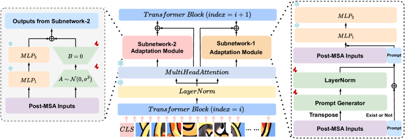
Figure 2: Comprehensive visualization of the generation and integration processes of the subnetwork-1 and subnetwork-2 adaptation modules within the transformer architecture.

Utilizing the pre-trained ViT architecture, our framework divides $B$ input images, denoted as $x$, into patch tokens of dimensionality $D$ and count $N$, further augmented with a class token $E_{CLS}$ to establish the initial sequence $I_{0}=[E_{CLS};E_{1}^{0},E_{2}^{0},\ldots,E_{N}^{0}]$. After transformation through the $i$-th transformer block, the sequence changes to:

$$I_{i}=[E_{CLS};E_{1}^{i},E_{2}^{i},\ldots,E_{N}^{i}]\in\mathbb{R}^{B\times(N+1)\times D}.$$ (10)

PEFT-CL methodologies typically employ a prompt pool or introduce auxiliary parameters while preserving pre-trained weights, modifying $E_{1}^{i},E_{2}^{i},\ldots,E_{N}^{i}$ within each transformer block to influence the class token $E_{CLS}$. This generates a novel feature space that adapts to sub-tasks and mitigates catastrophic forgetting. In these methods, the predetermined task prompt pool is traditionally used to derive task-specific embeddings, selecting prompts through cosine similarity [82, 81, 36]. While effective, this paradigm incurs substantial computational overhead when intervening in the self-attention mechanism and constrains the network’s capacity for generating diverse, instance-specific adaptive interventions dynamically. To address these limitations, our proposed NTK-CL framework implements a more efficient paradigm utilizing additional trainable parameters to autonomously generates instance-specific interventions. These interventions then interact with our proposed feature space post-multi-head self-attention (MSA) module to yield task-specific embeddings. This approach not only maximizes the utilization of pre-trained knowledge but also effectively reduces the computational burden brought by intervening MSA calculations.

The input to the adaptation modules post-MSA module is structured as follows:

$$u_{i}=MSA(I_{i})\in\mathbb{R}^{B\times(N+1)\times D}.$$ (11)

Next, we elucidate the generation processes for subnetwork-1 adaptation features, subnetwork-2 adaptation features, and hybrid adaptation features, which effectively triple the sample size in the feature space and reduce the generalization gaps in PEFT-CL training based on lemma 3.

Creating Subnetwork-1 Adaptation Features: To pinpoint the optimal interventions for enhancing the patch ($N+1$) dimensionality within transformer blocks, we deploy a specialized subnetwork-1 adaptation module $G_{S1}$. Tailored to the post-MSA inputs $u_{i}$, $G_{S1}$ adaptively transforms them into the most suitable prompts $q_{i}$ for this task, as illustrated in Fig. 2 (right).

$$q_{i}=G_{S1}(u_{i};q_{i-1})\in\mathbb{R}^{B\times(N+Q+1)\times D},$$ (12)

where $Q$ denotes the dimensionality of the prompts.

Delving into the details, within each transformer block, the prompt generator in $G_{S1}$ (as a fully connected layer) condenses the dimensional knowledge and adds it residually to the prompts generated in the previous transformer block, ensuring the integrity of the optimized information. The generated prompts $q_{i}$ are then concatenated with the input $u_{i}$ and subsequently passed into the pre-trained fully connected layers of the transformer block for continued optimization.

$$SAE_{i}^{1}=MLP_{2}(MLP_{1}([E_{CLS};q_{i};E_{1}^{i},E_{2}^{i},\ldots,E_{N}^{i}])),$$ (13)

where $SAE_{i}^{1}$ represents the subnetwork-1 adaptation embeddings generated by the $i$-th transformer block.

After passing through all transformer blocks, we extract the final optimized $SAE^{1}_{*}$ to obtain the subnetwork-1 adaptation features $E_{CLS}^{S1}$, thereby constructing a feature space suited to patch-level knowledge for this task.

Creating Subnetwork-2 Adaptation Features: To enrich the embedding landscape and foster knowledge acquisition, we integrate the LORA architecture [27] as the subnetwork-2 adaptation module $G_{S2}$. Designed for efficient fine-tuning of pre-trained models by minimizing parameter adjustments, LORA enables the mastering of extensive knowledge in compact, low-rank representations while preserving efficacy during high-dimensional reconstructions. Our implementation bifurcates into $G_{S2}^{low}$ for low-rank space mapping and $G_{S2}^{high}$ for reconversion to the high-dimensional space.

Employing the input $u_{i}$, $G_{S2}$ follows a procedure akin to the prompt generator in $G_{S1}$, generating the channel interventions $c_{i}$. However, unlike in $G_{S1}$, the generated $c_{i}$ does not pass through the pre-trained fully connected layers.

$$c_{i}=G_{S2}^{high}(G_{S2}^{low}(u_{i}))\in\mathbb{R}^{B\times(N+1)\times D}.$$ (14)

Considering that $c_{i}$ and processed $u_{i}$ by the pre-trained fully connected layers share identical dimensionalities, we opt for a summation rather than concatenation. This approach forms the subnetwork-2 adaptation embeddings $SAE^{2}_{i}$, streamlining the process and reducing computational overhead:

$$SAE^{2}_{i}=c_{i}\oplus MLP_{2}(MLP_{1}(u_{i}))\in\mathbb{R}^{B\times(N+1)\times D}.$$ (15)

Similarly, after passing through all transformer blocks, we also obtain the final optimized $SAE^{2}_{*}$, from which we extract the subnetwork-2 adaptation features that are most suitable for this task’s channel information, $E_{CLS}^{S2}$, constructing the corresponding feature space.

Synthesizing Hybrid Adaptation Features: The primary objective of PEFT adaptations across both subnetwork-1 and subnetwork-2 is to increase the sample size within each task subset, thereby reducing the generalization gaps. However, this approach presents a dilemma: which feature space should be used to construct the prototype classifier? Our solution is to leverage all available spaces and creates an intermediate space that integrates the strengths of both, thereby expanding the sample size further. We integrate these spaces by merging the best of both worlds, ensuring a comprehensive and robust feature representation.

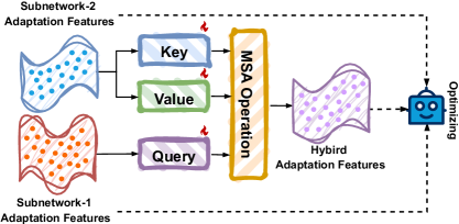
Figure 3: The illustration depicts the fusion of multi-level features to generate three distinct embeddings per sample, increasing the optimizable sample size.

Theorem 4 (Generalization in MSA).

Given an iteration horizon $K\geq 1$, consider any parameter vector $\boldsymbol{\theta}\in\mathbb{R}^{H(dT+d^{2})}$ and a number of attention heads $H$ satisfying:

$$\sqrt{H}\geq dT^{1/2}R^{5}\|\boldsymbol{\theta}\|_{2,\infty}\|\boldsymbol{\theta}-\boldsymbol{\theta}_{0}\|^{3}.$$ (16)

Here, $d$ specifies the dimensionality of the input features, while $T$ indicates the sequence length. $R$ is a constant inherent to the network’s architecture, and $\|\cdot\|_{2,\infty}$ represents the maximum $\ell_{2}$-norm across the various parameter matrices. Additionally, the step-size $\eta$ is required to comply with the following constraints:

$$\eta\leq\min\left\{1,\frac{1}{\rho(\boldsymbol{\theta})},\frac{\|\boldsymbol{\theta}-\boldsymbol{\theta}_{0}\|^{2}}{K\hat{L}(\boldsymbol{\theta})},\frac{\|\boldsymbol{\theta}-\boldsymbol{\theta}_{0}\|^{2}}{\hat{L}(\boldsymbol{\theta}_{0})}\right\},$$ (17)

where $\rho(\boldsymbol{\theta})$ denotes the spectral radius, approximated by:

$$\rho(\boldsymbol{\theta})\approx d^{3/2}T^{3/2}R^{13}\|\boldsymbol{\theta}\|_{2,\infty}^{2}\|\boldsymbol{\theta}-\boldsymbol{\theta}_{0}\|^{2}.$$ (18)

Then, at iteration $K$, the training loss $\hat{L}$ and the norm of the weight differences are bounded as follows:

$$\hat{L}(\boldsymbol{\theta}_{K})\leq\frac{1}{K}\sum_{k=1}^{K}\hat{L}(\boldsymbol{\theta}_{k})+2\hat{L}(\boldsymbol{\theta})+\frac{5\|\boldsymbol{\theta}-\boldsymbol{\theta}_{0}\|^{2}}{4\eta K},$$ (19)

$$\|\boldsymbol{\theta}_{K}-\boldsymbol{\theta}_{0}\|\leq 4\|\boldsymbol{\theta}-\boldsymbol{\theta}_{0}\|.$$ (20)

Furthermore, the expected generalization gap at iteration $K$ is constrained by:

$$\mathbb{E}\left[L(\boldsymbol{\theta}_{K})-\hat{L}(\boldsymbol{\theta}_{K})\right]\leq\frac{4}{n}\mathbb{E}\left[2K\hat{L}(\boldsymbol{\theta})+\frac{9\|\boldsymbol{\theta}-\boldsymbol{\theta}_{0}\|^{2}}{4\eta}\right],$$ (21)

where expectations are computed over the randomness of the training set, $n$ denotes the size of the dataset, and $L$ and $\hat{L}$ represent the empirical and population losses, respectively.

Drawing on insights from [14], we have refined elements of this work to develop theorem 4. This development definitively shows that the MSA module, under specified initialization conditions, offers robust generalization guarantees. Furthermore, the composition of the generalization gap and population loss aligns with our predefined standards: it is inversely proportional to the sample size, necessitates L2 regularization for bounded parameters, and mandates that patterns between samples be orthogonal with equal-energy means and exhibit NTK separability. This coherence reinforces the validity of our methodology and underpins our further innovations.

In our fusion architecture, the MSA module remains crucial for theoretical convergence and generalization optimization. Drawing inspiration from [11], we implement an advanced fusion strategy by using $E_{CLS}^{S2}$ as both the key and value, while $E_{CLS}^{S1}$ serves as the query within the MSA mechanism. This configuration facilitates dynamic knowledge interchange between components, yielding a hybrid adaptation feature $E_{CLS}^{HAE}$. This synergistic consolidation effectively doubles the MSA module’s input dimensionality, theoretically reducing the generalization gaps and allowing the empirical loss to closely approximate the population loss, thereby approaching optimal parameter estimates. Figure 3 illustrates this integration.

$$E_{CLS}^{HAE}=\text{Softmax}\left(\frac{Q(E_{CLS}^{S1})\cdot K(E_{CLS}^{S2})^{T}}{\sqrt{\text{head\_dim}}}\right)\cdot V(E_{CLS}^{S2}),$$ (22)

where $Q$, $K$, and $V$ represent the query, key, and value operations in the self-attention mechanism, respectively.

At this point, for each sample, we obtain three features in different feature spaces: subnetwork-1 adaptation feature ($E_{CLS}^{S1}$), subnetwork-2 adaptation feature ($E_{CLS}^{S2}$), and hybrid adaptation feature ($E_{CLS}^{HAE}$). Among them, $E_{CLS}^{HAE}$ is our preferred choice for constructing the prototype classifier.

Ultimately, by using these three features and their corresponding labels to construct a cross-entropy loss, we achieve a threefold expansion of the sample size within each finite task subset, effectively reducing generalization gaps:

$$\mathcal{L}_{cls}=CE(E_{CLS}^{S1},y)+CE(E_{CLS}^{S2},y)+CE(E_{CLS}^{HAE},y),$$ (23)

where $CE$ denotes the cross-entropy loss function, and $y$ indicates the corresponding labels.

5.2 Task-Level Feature Constraints

Informed by insights from theorem 1, our approach underscores that effectively reducing generalization gap involves the diligent preservation of historical knowledge $\Phi_{\tau}(X_{\tau},X_{\tau})$ and $\Phi_{k}(X_{k},X_{k})$ from the perspective of the task $T$, coupled with a concerted effort to diminish cross-task interactions $\Phi_{k}(X_{\tau},X_{k})$, for $k>\tau$. Given $\Phi_{k}(X_{\tau},X_{k})=\frac{\partial f_{k}^{*}(X_{\tau})}{\partial p_{k}}\frac{\partial f_{k}^{*}(X_{k})}{\partial p_{k}}$, if the difference between $f_{k}^{*}(X_{\tau})$ and $f_{k}^{*}(X_{k})$ is maximized, then $\Phi_{k}(X_{\tau},X_{k})$ will be minimized. Since $p_{k}$ in the optimization process of PEFT-CL will only be influenced by $f_{k}^{*}(X_{k})$, ensuring orthogonality between $f_{k}^{*}(X_{\tau})$ and $f_{k}^{*}(X_{k})$ will make $\frac{\partial f_{k}^{*}(X_{\tau})}{\partial p_{k}}$ extremely small [16]. However, in the practical setting of PEFT-CL, cross-task access to data is strictly prohibited, presenting a substantial challenge in maintaining task-level distinctiveness.

Therefore, we propose a compromise approach. Within the context of NTK theory, the optimization of infinitely wide neural networks mirrors a Gaussian process [10, 40], yielding a locally constant NTK matrix [32, 91, 42, 12]. Given this, it is reasonable to assume that $\Phi^{*}(X_{\tau},X_{k})=\Phi_{0}(X_{\tau},X_{k})=\Phi_{1}(X_{\tau},X_{k})=\cdots=\Phi_{\infty}(X_{\tau},X_{k})$. Moreover, networks pre-trained on extensive datasets emulate the properties of infinitely wide networks [41, 83, 75], aligning with our pre-trained model. Therefore, we relax the original constraint, assuming that the pre-trained model is at this local optimum.

Under this framework, $\Phi_{k}(X_{\tau},X_{k})\approx\Phi^{*}(X_{\tau},X_{k})=\frac{\partial f^{*}(X_{\tau})}{\partial p}\cdot\frac{\partial f^{*}(X_{k})}{\partial p}$, suggesting that ensuring orthogonality between $f^{*}(X_{\tau})$ and $f^{*}(X_{k})$ is feasible to some extent. To practically achieve this, integrating a prototype classifier and imposing orthogonality constraints ensure that embeddings from different tasks remain distinct, thus not violating the constraints under the PEFT-CL scenarios and aligning with the objective to minimize generalization gap.

Knowledge Retention: Effective replay of past knowledge is essential in PEFT-CL utilizing pre-trained models. For instance, [77] employs a distributional strategy that approximates and replays past data distributions for ongoing optimization, while [100] preserves distinct adapter parameters for each historical task. These strategies, while boosting knowledge retention, simultaneously escalate optimization and storage requirements, posing challenges to scalability and operational efficiency in scenarios with large datasets or extensive task sequences. To mitigate these issues, we introduce an adaptive Exponential Moving Average (EMA) mechanism tailored for efficient past knowledge preservation, illustrated in Fig. 4.

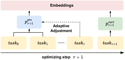
Figure 4: Leveraging the adaptive EMA mechanism, we meticulously maintain a repository of visual summaries from the adaptation modules’ parameters of prior tasks. The resulting network embedding is bifurcated into two distinct components: the pre-embedding, which retains historical knowledge, and the curr-embedding, which captures current insights. These segments are concatenated to create a composite embedding, ensuring a comprehensive representation that integrates past and present knowledge seamlessly.

Traditional EMA applications often maintain a static base model, incrementally integrating optimized weights to preserve historical data. However, this approach proves suboptimal in PEFT-CL settings due to the substantial disparities in weights across tasks. Directly preserving a large proportion of past weights can detrimentally affect the performance on current tasks, while retaining an entire model’s weights is excessively redundant. Therefore, we propose two improvements. First, we categorize the adaptation parameters responsible for generating embedding into two segments: $p^{pre}$ for historical knowledge and $p^{curr}$ for current insights. Secondly, we apply the EMA mechanism exclusively to the adaptation modules’ parameters, leaving other optimizable parameters untouched to ensure the optimization remains streamlined. Throughout the optimization of task $\tau+1$, only $p^{curr}_{\tau+1}$ is modified, while $p^{pre}_{\tau+1}$ is adaptively adjusted post-task-$\tau$ completion, employing an adaptive EMA scheme:

$$[k_{1}(n),k_{2}(n)]=\begin{cases}[0,1]&\text{if }n=0\\ [\frac{1}{{n+1}}\cdot\frac{1}{k_{2}(n-1)},\frac{1}{{n+1}}]&\text{otherwise}\end{cases}$$ (24)

$$p^{pre}_{\tau+1}=k_{1}(\tau)p^{pre}_{\tau}+k_{2}(\tau)p^{curr}_{\tau}.$$ (25)

Under this mechanism, each past task equitably contributes to constructing embeddings related to historical knowledge without compromising the current tasks’ insights, while avoiding the excessive memory overhead of storing parameters for each task, as seen in [100]. Consequently, $E_{CLS}^{S1}$, $E_{CLS}^{S2}$, and $E_{CLS}^{HAE}$ all consist of two components: $concat[f(x,p_{pre}),f(x,p_{curr})]$.

Task-Feature Dissimilarity: Based on Sect. 5.2 and insights from [16, 3], it is evident that achieving orthogonal insulation between $f^{*}(X_{\tau})$ and $f^{*}(X_{k})$ can compromise to reduce generalization gap. Therefore, relying on the prototype classifier, we propose an optimization loss. In line with [100, 77], we update the prototype classifier $\zeta$ upon completion of each task’s optimization and strictly prohibit accessing previous samples in subsequent optimizations to comply with PEFT-CL constraints. During the optimization of task $\tau$, we randomly sample $\zeta_{\tau}$ from $\zeta$ to represent $f^{*}(X_{\tau})$ . To initially distinguish $f^{*}(X_{\tau})$ from $f^{*}(X_{k})$, we use the InfoNCE [57] as a metric, employing $\zeta_{\tau}$ as the negative sample, while using samples $x_{\tau}$ (represented by $E_{CLS}^{HAE}$, as this is the feature used for final classification) from task $\tau$ as positive samples.

$$\mathcal{L}_{dis}=-\frac{1}{|x_{\tau}|}\sum_{i\in|x_{\tau}|}\log\frac{\exp(\text{sim}(z_{i},c_{i}))}{\sum_{j\in|\zeta_{\tau}|}\exp(\text{sim}(z_{i},c_{j}))},$$ (26)

where $|x_{\tau}|$ represents the number of positive samples, $|\zeta_{\tau}|$ denotes the number of negative samples, $z_{i}$ and $c_{i}$ are the same-class positive samples used for optimization, and $z_{j}$ is the negative samples sampled from the prototype classifier.

To further ensure orthogonality between $f^{*}(X_{\tau})$ and $f^{*}(X_{k})$, we apply the truncated SVD method [21] to constrain the optimization of $f^{*}(X_{k})$. Specifically, we decompose $\zeta$ to obtain the orthogonal basis $\mathbf{U}$ that defines the classification (preceding feature) space. We then map $x_{\tau}$ into this space and remove the unmappable part from the original $x_{\tau}$. When the retained mappable portion is sufficiently small, the orthogonality between $x_{\tau}$ and $\zeta$ is ensured, thus maintaining orthogonality.

$$\mathcal{L}_{\text{orth}}=\sum_{i\in|x_{\tau}|}\|z_{i}-\tilde{proj}(z_{i},U)\|_{2}^{2},$$ (27)

where $\tilde{proj}(a,b)$ is the unmappable portion of $a$ in the space formed by the orthogonal basis functions decomposed from $b$.

5.3 Regularization Adjustment

In accordance with the theoretical constraints delineated in Appendix A, which advocate for the incorporation of ridge regression to ensure a well-conditioned solution, we deploy an L2 regularization [28]. As specified in Eq. 32, the regularization term is structured as $\left\|p_{\tau}-p_{\tau-1}^{*}\right\|_{2}^{2}$, targeting the parameter shifts from task $\tau-1$ to task $\tau$. Consequently, we meticulously design our regularization term to mirror this structure and temporarily retain the trainable parameters $p^{pre}$ from the preceding task. This targeted regularization is then precisely applied to the parameters of the various modules within our NTK-CL, formulated as follows:

$$\small\mathcal{L}_{\text{reg}}=\|p_{G_{S1}}^{curr}-p_{G_{S1}}^{pre}\|_{2}^{2}+\|p_{G_{S2}}^{curr}-p_{G_{S2}}^{pre}\|_{2}^{2}+\|p_{G_{H}}^{curr}-p_{G_{H}}^{pre}\|_{2}^{2},$$ (28)

where $G_{S1}$, $G_{S2}$, and $G_{H}$ represent the trainable parameters of the subnetwork-1 adaptation module, the subnetwork-2 adaptation module, and the hybrid adaptation module.

Training Optimization: The composite objective for optimizing the training of each task subset within our NTK-CL is rigorously defined as follows:

$$\mathcal{L}=\mathcal{L}_{cls}+\eta\mathcal{L}_{dis}+\upsilon\mathcal{L}_{orth}+\lambda\mathcal{L}_{reg},$$ (29)

where $\eta$ and $\upsilon$ are hyper-parameters, meticulously calibrated to maximize task-feature dissimilarity and to promote orthogonality in task-feature representations, respectively. The parameter $\lambda$ controls the intensity of the regularization, ensuring the model’s robustness and generalizability.

Prototype Classifier: Upon the completion of each task’s training, we conduct an averaging operation on the features generated by all classes involved in that task to update the classifier $\zeta$ with the most representative features of each class. It is important to note that the features used at this stage are designated as hybrid adaptation features $E_{CLS}^{HAE}$.

$$\zeta_{i}=\frac{1}{N_{i}}\sum_{j=1}^{N_{i}}E_{CLS,ij}^{HAE},$$ (30)

where $N_{i}$ denotes the number of feature vectors for class $i$ within the task, and $E_{CLS,ij}^{HAE}$ represents the hybrid adaptation feature vector of the $j$-th sample in class $i$.

Upon updating all class features within the task in the prototype classifier $\zeta$, the system transitions to training the subsequent task. During this new training phase, there is a strict prohibition on accessing data from previous tasks, reinforcing the integrity of the continual learning process.

Testing Evaluation: Upon concluding the training regimen, the evaluation phase commences with simultaneous testing across all tasks. This phase distinctly prioritizes the synthesized hybrid adaptation features $E_{CLS}^{HAE}$ for final analysis. Through the final prototype classifier $\zeta$, these features are transformed into logits, which are subsequently aligned with the corresponding labels to deduce the test accuracy.

TABLE I: Summary of datasets for the PEFT-CL settings, detailing task counts, class counts, image totals, and domains.

Dataset	Task	Class	Image	Domain
CIFAR-100	10	100	60000	Object Recognition
ImageNet-R	10	200	30000	Object Recognition
ImageNet-A	10	200	7500	Object Recognition
DomainNet	15	345	423506	Domain Adaptation
Oxford Pets	7	37	7393	Animal Recognition
EuroSAT	5	10	27000	Earth Observation
PlantVillage	5	15	20638	Agricultural Studies
VTAB	5	50	10415	Task Adaptation
Kvasir	4	8	4000	Healthcare Diagnosis

6 Experiments

Datasets: In our empirical analysis, we utilize a comprehensive collection of datasets, meticulously curated to rigorously evaluate the model’s adaptability within the PEFT-CL scenarios. These datasets span a broad spectrum of domains, including general object recognition, domain adaptation, animal recognition, and geospatial analysis, providing a robust framework for assessment. Below, we elucidate the significance, structure, and relevance of each dataset to our investigation:

CIFAR-100 [38]: This dataset, crucial for assessing continual learning algorithms, comprises 60,000 32x32 color images across 100 classes, with each class contributing 600 images. For PEFT-CL, it is segmented into 10 distinct tasks, each encompassing 10 classes. Images are resized to 224x224 to be compatible with the pre-trained ViT model.

ImageNet-R [81]: It enriches the original ImageNet dataset by incorporating artworks, cartoons, and interpretations for 200 classes. This dataset underscores the challenge of generalizing across highly varied visual domains. For our evaluation, the ImageNet-R is organized into 10 tasks, each containing 20 classes, with a distribution of 24,000 training images and 6,000 test images, offering a rigorous testbed for assessing model generalization in complex PEFT-CL scenarios.

ImageNet-A [25]: This challenging dataset is an extension of ImageNet, curated to evaluate model robustness against adversarial and out-of-distribution samples. It contains 7,500 images from 200 classes, each designed to be misclassified by standard models. For PEFT-CL, ImageNet-A is divided into 10 tasks, providing a stringent test of a model’s ability to handle challenging and unusual cases, thereby assessing resilience and generalization in continual learning scenarios.

DomainNet [59]: This large-scale domain adaptation dataset includes six domains: Clipart, Infograph, Painting, Quickdraw, Real, and Sketch, comprising 423,506 images across 345 categories. For PEFT-CL, it is divided into 15 tasks, each containing 23 classes, to rigorously test cross-domain generalization capabilities. Our study expands beyond previous research like DAP [36], which focused solely on the Real domain, and CODA-Prompt [71], which limited its investigation to a five-task sequence within the Real domain. By encompassing all six domains in a structured 15-task framework, we provide a comprehensive assessment of domain adaptation within the CL context, establishing a new benchmark in this research area.

Moving beyond conventional datasets utilized in CL research, our study integrates a wide array of datasets from diverse domains, encompassing object recognition, domain adaptation, animal recognition, earth observation, agricultural studies, task adaptation, and healthcare diagnosis. We employ datasets such as Oxford Pets [58], EuroSAT [24], PlantVillage [30], VTAB [98], and Kvasir [61], as summarized in Table I. This comprehensive dataset selection underscores our model’s robustness, extensive generalization, and adaptability across a spectrum of visual recognition tasks, thereby reinforcing its capability to address varied domain-specific challenges.

Training Details: Experiments are conducted on NVIDIA RTX 4090 GPUs, with all methods implemented in PyTorch, consistent with the protocols in [82]. We utilize two configurations of the ViT: ViT-B/16-IN21K and ViT-B/16-IN1K, with the latter being fine-tuned on ImageNet-1K, as our foundational models. In our NTK-CL setup, the SGD optimizer is used for training across 20 epochs with a batch size of 16. The learning rate starts at 0.01, adjusting via cosine annealing to promote optimal convergence.

Evaluation Metrics: Following the established benchmark protocol as outlined by [66], we evaluate the model’s effectiveness using $A_{\tau}$, which signifies the accuracy post the $\tau$-th training stage. Notably, we employ $A_{T}$—the performance metric at the termination of the final stage—and $\bar{A}=\frac{1}{T}\sum_{\tau=1}^{T}A_{\tau}$, which calculates the average accuracy over all incremental stages. These metrics are selected as the principal measures of model performance, providing a holistic view of its efficacy and stability throughout the training process.

TABLE II: Comparative performance analysis in PEFT-CL using ViT-Base16, pre-trained on ImageNet-21K, as the foundational model. Bold segments indicate optimal results, while underlined segments denote suboptimal results.

Method	Publisher	CIFAR-100		ImageNet-R		ImageNet-A
		$\bar{A}$ (%)	$A_{T}$ (%)	$\bar{A}$ (%)	$A_{T}$ (%)	$\bar{A}$ (%)	$A_{T}$ (%)
L2P [82]	CVPR 2022	89.30 $\pm$ 0.34	84.16 $\pm$ 0.72	72.38 $\pm$ 0.89	65.57 $\pm$ 0.67	47.86 $\pm$ 1.26	38.08 $\pm$ 0.79
DualPrompt [81]	ECCV 2022	90.68 $\pm$ 0.21	85.76 $\pm$ 0.45	72.45 $\pm$ 0.94	66.31 $\pm$ 0.55	52.16 $\pm$ 0.83	40.07 $\pm$ 1.69
CODA-Prompt [71]	CVPR 2023	91.36 $\pm$ 0.18	86.70 $\pm$ 0.28	77.16 $\pm$ 0.65	71.59 $\pm$ 0.53	56.13 $\pm$ 2.51	45.34 $\pm$ 0.92
EvoPrompt [39]	AAAI 2024	92.06 $\pm$ 0.37	87.78 $\pm$ 0.63	78.84 $\pm$ 1.13	73.60 $\pm$ 0.39	54.88 $\pm$ 1.21	44.31 $\pm$ 0.88
OVOR [29]	ICLR 2024	91.11 $\pm$ 0.38	86.36 $\pm$ 0.38	75.63 $\pm$ 1.08	70.48 $\pm$ 0.19	53.33 $\pm$ 1.11	42.88 $\pm$ 0.67
L2P-PGP [62]	ICLR 2024	89.61 $\pm$ 0.64	84.23 $\pm$ 0.87	74.91 $\pm$ 1.50	68.06 $\pm$ 0.46	50.57 $\pm$ 0.15	39.75 $\pm$ 1.02
CPrompt [19]	CVPR 2024	91.58 $\pm$ 0.52	87.17 $\pm$ 0.32	81.02 $\pm$ 0.33	75.30 $\pm$ 0.57	60.10 $\pm$ 1.34	49.78 $\pm$ 0.87
EASE [100]	CVPR 2024	92.58 $\pm$ 0.48	88.11 $\pm$ 0.67	81.92 $\pm$ 0.48	76.04 $\pm$ 0.19	64.35 $\pm$ 1.41	54.64 $\pm$ 0.70
InfLoRA [48]	CVPR 2024	91.96 $\pm$ 0.24	86.93 $\pm$ 0.90	81.63 $\pm$ 0.82	75.53 $\pm$ 0.53	55.50 $\pm$ 0.85	44.21 $\pm$ 1.77
NTK-CL (Ours)	-	93.76 $\pm$ 0.35	90.27 $\pm$ 0.20	82.77 $\pm$ 0.66	77.17 $\pm$ 0.19	66.56 $\pm$ 1.53	58.54 $\pm$ 0.91

TABLE III: Comparative performance analysis in PEFT-CL using the ViT-Base16, fine-tuned on ImageNet-1K, as the foundational model. Bold segments indicate optimal results, while underlined segments denote suboptimal results.

Method	Publisher	CIFAR-100		ImageNet-R		ImageNet-A
		$\bar{A}$ (%)	$A_{T}$ (%)	$\bar{A}$ (%)	$A_{T}$ (%)	$\bar{A}$ (%)	$A_{T}$ (%)
L2P [82]	CVPR 2022	87.86 $\pm$ 0.23	81.62 $\pm$ 0.75	72.38 $\pm$ 0.89	65.57 $\pm$ 0.67	53.42 $\pm$ 0.95	44.98 $\pm$ 1.31
DualPrompt [81]	ECCV 2022	88.96 $\pm$ 0.36	83.50 $\pm$ 0.67	72.45 $\pm$ 0.94	66.31 $\pm$ 0.55	57.56 $\pm$ 1.02	47.85 $\pm$ 0.47
CODA-Prompt [71]	CVPR 2023	91.22 $\pm$ 0.48	86.43 $\pm$ 0.23	77.67 $\pm$ 1.36	72.00 $\pm$ 1.33	61.28 $\pm$ 0.90	51.80 $\pm$ 0.79
EvoPrompt [39]	AAAI 2024	91.89 $\pm$ 0.45	87.56 $\pm$ 0.23	81.43 $\pm$ 1.07	75.86 $\pm$ 0.33	58.46 $\pm$ 1.10	48.13 $\pm$ 0.38
OVOR [29]	ICLR 2024	89.50 $\pm$ 0.60	84.26 $\pm$ 0.60	78.61 $\pm$ 1.00	73.18 $\pm$ 0.49	59.50 $\pm$ 1.00	50.10 $\pm$ 1.00
L2P-PGP [62]	ICLR 2024	89.49 $\pm$ 0.48	84.63 $\pm$ 0.40	72.05 $\pm$ 0.85	66.42 $\pm$ 0.57	47.28 $\pm$ 1.23	39.21 $\pm$ 0.93
CPrompt [19]	CVPR 2024	91.74 $\pm$ 0.43	87.51 $\pm$ 0.38	82.20 $\pm$ 0.89	76.77 $\pm$ 0.64	55.07 $\pm$ 20.79	46.99 $\pm$ 17.03
EASE [100]	CVPR 2024	91.88 $\pm$ 0.48	87.45 $\pm$ 0.34	82.59 $\pm$ 0.70	77.12 $\pm$ 0.23	67.36 $\pm$ 0.94	58.28 $\pm$ 0.82
InfLoRA [48]	CVPR 2024	91.47 $\pm$ 0.65	86.44 $\pm$ 0.47	82.50 $\pm$ 1.00	76.68 $\pm$ 0.60	58.65 $\pm$ 1.39	47.31 $\pm$ 0.99
NTK-CL (Ours)	-	93.16 $\pm$ 0.46	89.43 $\pm$ 0.34	83.18 $\pm$ 0.40	77.76 $\pm$ 0.25	68.76 $\pm$ 0.71	60.58 $\pm$ 0.56

TABLE IV: Performance analysis in the PEFT-CL context utilizes ViT-Base16, pre-trained on ImageNet-21K, across various datasets. The bold segments denote optimal results, and the underlined segments indicate suboptimal outcomes.

Method	Publisher	DomainNet		Oxford Pets		EuroSAT
		$\bar{A}$ (%)	$A_{T}$ (%)	$\bar{A}$ (%)	$A_{T}$ (%)	$\bar{A}$ (%)	$A_{T}$ (%)
OVOR [29]	ICLR 2024	75.80 $\pm$ 0.40	68.77 $\pm$ 0.12	91.56 $\pm$ 1.87	84.08 $\pm$ 1.37	78.97 $\pm$ 3.71	63.24 $\pm$ 5.22
EASE [100]	CVPR 2024	71.82 $\pm$ 0.49	65.42 $\pm$ 0.14	94.71 $\pm$ 1.79	89.97 $\pm$ 1.56	87.61 $\pm$ 2.36	77.73 $\pm$ 2.41
InfLoRA [48]	CVPR 2024	69.74 $\pm$ 0.31	57.35 $\pm$ 0.32	59.46 $\pm$ 0.80	29.15 $\pm$ 1.04	81.82 $\pm$ 3.27	70.04 $\pm$ 5.78
NTK-CL (Ours)	-	73.70 $\pm$ 0.47	67.44 $\pm$ 0.36	96.69 $\pm$ 0.99	94.11 $\pm$ 0.09	87.63 $\pm$ 2.32	79.84 $\pm$ 0.32
Additional Datasets		PlantVillage		VTAB		Kvasir
OVOR [29]	ICLR 2024	81.08 $\pm$ 2.73	65.96 $\pm$ 3.93	85.14 $\pm$ 3.14	77.55 $\pm$ 3.36	77.27 $\pm$ 2.28	58.3 $\pm$ 2.69
EASE [100]	CVPR 2024	88.79 $\pm$ 4.43	80.92 $\pm$ 6.18	89.81 $\pm$ 1.68	84.76 $\pm$ 1.10	84.35 $\pm$ 2.22	69.32 $\pm$ 5.35
InfLoRA [48]	CVPR 2024	88.61 $\pm$ 4.23	80.34 $\pm$ 5.72	85.04 $\pm$ 2.21	78.17 $\pm$ 3.69	80.62 $\pm$ 1.70	59.0 $\pm$ 4.13
NTK-CL (Ours)	-	88.00 $\pm$ 2.37	81.88 $\pm$ 0.25	89.67 $\pm$ 1.88	85.53 $\pm$ 0.81	90.03 $\pm$ 0.73	82.7 $\pm$ 0.55

TABLE V: Performance analysis in the PEFT-CL context utilizes ViT-Base16, fine-tuned on ImageNet-1K, across various datasets. The bold segments denote optimal results, and the underlined segments indicate suboptimal outcomes.

Method	Publisher	DomainNet		Oxford Pets		EuroSAT
		$\bar{A}$ (%)	$A_{T}$ (%)	$\bar{A}$ (%)	$A_{T}$ (%)	$\bar{A}$ (%)	$A_{T}$ (%)
OVOR [29]	ICLR 2024	71.92 $\pm$ 0.41	63.87 $\pm$ 0.81	90.47 $\pm$ 1.51	82.85 $\pm$ 1.72	78.67 $\pm$ 2.74	62.88 $\pm$ 7.41
EASE [100]	CVPR 2024	71.30 $\pm$ 0.50	64.84 $\pm$ 0.13	94.94 $\pm$ 1.60	90.16 $\pm$ 1.48	91.06 $\pm$ 0.76	82.77 $\pm$ 2.15
InfLoRA [48]	CVPR 2024	69.19 $\pm$ 0.31	56.66 $\pm$ 0.33	58.71 $\pm$ 1.55	28.36 $\pm$ 1.89	82.12 $\pm$ 2.00	71.94 $\pm$ 6.09
NTK-CL (Ours)	-	72.94 $\pm$ 0.27	66.73 $\pm$ 0.21	96.62 $\pm$ 0.75	94.28 $\pm$ 0.09	88.50 $\pm$ 2.61	80.94 $\pm$ 0.30
Additional Datasets		PlantVillage		VTAB		Kvasir
OVOR [29]	ICLR 2024	80.74 $\pm$ 2.70	65.14 $\pm$ 4.21	84.87 $\pm$ 3.57	76.02 $\pm$ 2.96	76.84 $\pm$ 3.91	56.48 $\pm$ 2.97
EASE [100]	CVPR 2024	88.50 $\pm$ 4.55	80.75 $\pm$ 5.68	88.45 $\pm$ 1.69	82.55 $\pm$ 2.02	84.30 $\pm$ 1.39	69.65 $\pm$ 3.51
InfLoRA [48]	CVPR 2024	87.98 $\pm$ 4.54	81.54 $\pm$ 4.69	86.99 $\pm$ 2.74	78.19 $\pm$ 3.01	77.50 $\pm$ 5.19	58.72 $\pm$ 9.12
NTK-CL (Ours)	-	87.26 $\pm$ 2.16	80.81 $\pm$ 0.22	88.48 $\pm$ 2.25	83.47 $\pm$ 1.90	91.88 $\pm$ 1.15	84.72 $\pm$ 0.40

TABLE VI: Ablation study on the ViT-B/16-IN21K model, evaluating its performance across the CIFAR100 and ImageNet-R datasets. The study features a detailed breakdown of model components, denoted in each column by the inclusion (✓) of specific modules and strategies: Subnetwork-1 Adaptation Module (S1), Subnetwork-2 Adaptation Module (S2), Hybrid Adaptation Module (Hybrid), Knowledge Retention (KR), Task-Feature Dissimilarity Loss (Dis), Orthogonality Loss (Orth), and Regularization Loss (Reg). Incremental accuracies ($\bar{A}$) are reported to highlight their respective impacts on model performance.

Frozen ViT-B/16-IN21K on CIFAR100

Frozen ViT-B/16-IN21K on ImageNet-R

Adaptation Modules

Task Constraints

Regularization

$\bar{A}$ (%)

Adaptation Modules

Task Constraints

Regularization

$\bar{A}$ (%)

S1

S2

Hybrid

KR

Dis

Orth

Reg

S1

S2

Hybrid

KR

Dis

Orth

Reg

✓

82.99

✓

69.62

✓

✓

85.45 $\uparrow$+2.96%

✓

✓

70.45 $\uparrow$+1.19%

✓

85.04

✓

68.93

✓

✓

91.37 $\uparrow$+7.44%

✓

✓

77.77 $\uparrow$+12.82%

✓

86.51

✓

71.93

✓

✓

89.50 $\uparrow$+3.46%

✓

✓

77.50 $\uparrow$+7.74%

✓

✓

✓

89.47

✓

✓

✓

76.13

✓

✓

✓

✓

92.01 $\uparrow$+2.84%

✓

✓

✓

✓

81.08 $\uparrow$+6.50%

✓

✓

✓

✓

✓

93.32 $\uparrow$+4.30%

✓

✓

✓

✓

✓

82.55 $\uparrow$+8.43%

✓

✓

✓

✓

✓

92.39 $\uparrow$+3.26%

✓

✓

✓

✓

✓

81.10 $\uparrow$+6.53%

✓

✓

✓

✓

✓

92.39 $\uparrow$+3.26%

✓

✓

✓

✓

✓

81.42 $\uparrow$+6.95%

✓

✓

✓

✓

✓

✓

93.47 $\uparrow$+4.47%

✓

✓

✓

✓

✓

✓

82.62 $\uparrow$+8.52%

✓

✓

✓

✓

✓

✓

✓

93.72 $\uparrow$+4.75%

✓

✓

✓

✓

✓

✓

✓

82.85 $\uparrow$+8.83%

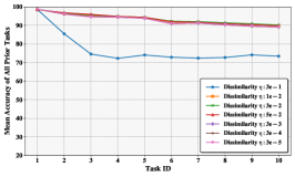
(a) CIFAR100-$\eta$ Tuning

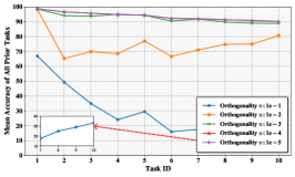
(b) CIFAR100-$\upsilon$ Tuning

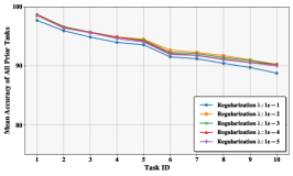
(c) CIFAR100-$\lambda$ Tuning

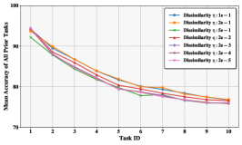
(d) ImageNet-R-$\eta$ Tuning

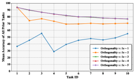
(e) ImageNet-R-$\upsilon$ Tuning

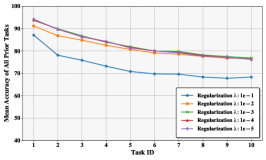
(f) ImageNet-R-$\lambda$ Tuning

Figure 5: Illustration of the tuning process for each hyper-parameter on CIFAR100 and ImageNet-R, showing the continuous performance variations.

6.1 Benchmark Comparison

In this subsection, we evaluate the NTK-CL method against other leading approaches. To ensure a fair performance comparison, we fix random seeds from 0 to 4, ensuring consistent task segmentation for each run . We utilize uniformly sourced pre-trained weights and maintain the optimal hyper-parameters from the open-source code without modifications. Performance metrics for major datasets using ImageNet-21K pre-trained weights and ImageNet-1K fine-tuned weights are presented in Tables II and III.

For primary datasets such as CIFAR100, ImageNet-R, and ImageNet-A, we assess our method against most contemporary approaches, excluding DAP [36] due to its flawed testing process, Hide-Prompt [77] which compresses and samples past data, and Dual-PGP [62] which requires specific instance counts. By controlling for confounding factors, our method consistently achieves state-of-the-art performance. The NTK-CL method exhibits a clear advantage in both incremental accuracy ($\bar{A}$) and final accuracy ($A_{T}$), with improvements ranging from 1% to 7% compared to methods such as EASE [100] and EvoPrompt [39]. This advantage is particularly significant on ImageNet-A, a dataset known for challenging traditional models. Our approach substantially enhances model generalization and demonstrates robustness in complex visual recognition tasks.

Additionally, performance on auxiliary datasets including DomainNet, Oxford Pets, EuroSAT, PlantVillage, VTAB, and Kvasir, as detailed in Tables IV and V, highlights the generalization and adaptability of NTK-CL across diverse domains. On these datasets, NTK-CL not only consistently delivers superior accuracy metrics but also exhibits reduced variance in performance, emphasizing its stability. Notably, on Oxford Pets, NTK-CL achieves incremental accuracy improvements ranging from 1.8% to 2.1% and final accuracy enhancements of up to 4.6% compared to EASE [100]. On the Kvasir dataset, NTK-CL outperforms competing methods, achieving the highest incremental accuracy improvements ranging from 6.7% to 9.0% and the highest final accuracy improvements ranging from 19.3% to 21.1%, showcasing its significant potential for medical applications. Across other datasets, NTK-CL consistently ranks as the best or the second-best, further affirming the method’s efficacy and versatility. In conclusion, NTK-CL establishes a new benchmark in PEFT-CL, demonstrating superior performance across a diverse array of datasets.

6.2 Ablation Study

To ensure rigorous alignment between theoretical frameworks and empirical validation, a comprehensive suite of ablation studies is executed using the CIFAR100 and ImageNet-R datasets. Experimental conditions are standardized by setting the random seed to 0, ensuring consistent task segmentations, and utilizing weights from ViT-B/16-IN21K to maintain model consistency. The ablation studies encompass various configurations, including the Subnetwork-1 Adaptation Module (S1), Subnetwork-2 Adaptation Module (S2), Hybrid Adaptation Module (Hybrid), Knowledge Retention (KR), Task-Feature Dissimilarity Loss (Dis), Orthogonality Loss (Orth), and Regularization Loss (Reg). Average task-related accuracies ($\bar{A}$) are assessed to critically analyze their individual contributions to the model’s overall performance, which is displayed in Table VI.

Initial evaluations focus on the merits and drawbacks of S1, S2, and Hybrid modules, along with the benefits of their joint optimization. Experimental results across various datasets consistently demonstrate that the Hybrid module outperforms both S1 and S2 modules by effectively leveraging their combined strengths. Joint optimization leads to significant performance enhancement, affirming the generalization gains linked to increased sample size, which inherently supports knowledge transfer and retention in PEFT-CL.

The impact of the KR module across various adaptation module configurations is systematically explored to elucidate its influence on model performance. Implementing the KR module with the S1, S2, and Hybrid adaptation modules demonstrates substantial improvements in task-related accuracies ($\bar{A}$). Specifically, integrating the KR module increases the $\bar{A}$ from 82.99% to 85.45% on CIFAR100 and from 69.62% to 70.45% on ImageNet-R for the S1 configuration. For the S2 configuration, the $\bar{A}$ enhancement is more pronounced, rising from 85.04% to 91.37% on CIFAR100 and from 68.93% to 77.77% on ImageNet-R. The Hybrid module also benefits significantly, with increases from 86.51% to 89.50% on CIFAR100 and from 71.93% to 77.50% on ImageNet-R. A combined configuration of all three adaptation modules further raises the $\bar{A}$ to 92.01% on CIFAR100 and 81.08% on ImageNet-R, underscoring the KR module’s effectiveness in fostering knowledge retention and substantially boosting model generalization across diverse settings. It is noteworthy that while the KR module significantly enhances the performance of subnetwork-2 adaptation features, their potential remains limited compared to the jointly optimized hybrid features.

Further, the impact of task-feature dissimilarity losses is assessed, demonstrating that integrating Dis into the configuration results in $\bar{A}$ of 93.32% on CIFAR100 and 82.55% on ImageNet-R, showing enhancements of 4.30% and 8.43%. Additionally, the inclusion of Orth alongside the three adaptation modules and the KR module leads to an $\bar{A}$ of 92.39% on CIFAR100 and 81.10% on ImageNet-R, reflecting gains of 3.26% and 6.53%, respectively. These findings further emphasize the significant role of task-feature dissimilarity losses in PEFT-CL.

Finally, incorporating Reg within the same configuration results in an $\bar{A}$ of 92.39% on CIFAR100 and an enhanced $\bar{A}$ of 81.42% on ImageNet-R, indicating improvements of 3.26% and 6.95%, respectively. When all components and strategies are integrated, the model achieves the highest $\bar{A}$ values of 93.72% on CIFAR100 and 82.85% on ImageNet-R, reflecting cumulative enhancements of 4.75% and 8.83%.

Therefore, as summarized above, through these detailed ablation studies, we have demonstrated our theoretical derivations from a practical standpoint and ensured that each aspect of our design is rational and effective.

	Original	Task-0	Task-1	Task-2	Task-3	Task-4	Task-5	Task-6	Task-7	Task-8	Task-9
ViT-21K
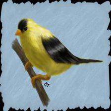
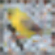
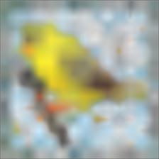
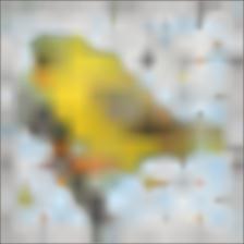
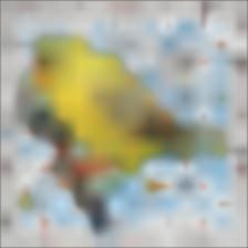
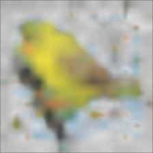
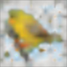
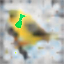
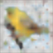
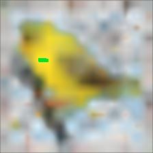
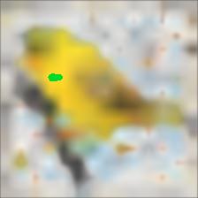
S1
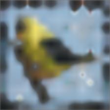
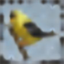
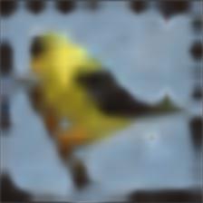
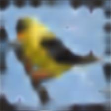
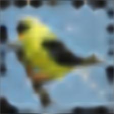
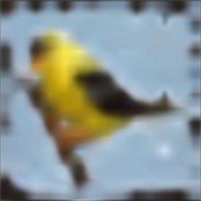
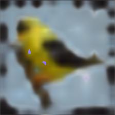
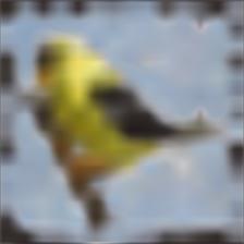
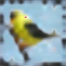
S2

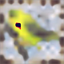
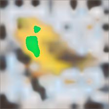
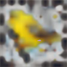
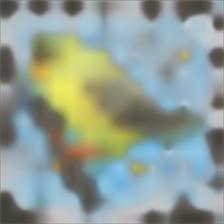
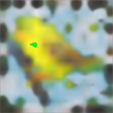
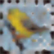
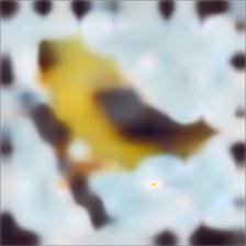
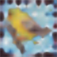
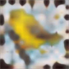
Figure 6: The illustration showcases DIP visualizations for the painted serinus canaria in ImageNet-R. The first row features images generated at each task period using embeddings from the ImageNet-21K pre-trained model. The second and third rows display images produced by embeddings from the Subnetwork-1 (S1) Adaptation Module and the Subnetwork-2 (S2) Adaptation Module, respectively.

	Original	Task-0	Task-1	Task-2	Task-3	Task-4	Task-5	Task-6	Task-7	Task-8	Task-9
ViT-21K
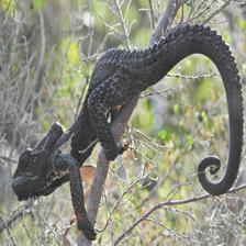
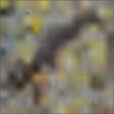
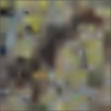
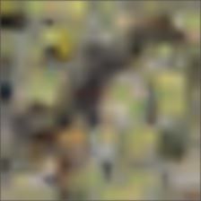
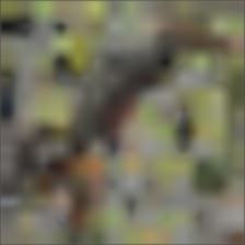
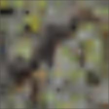
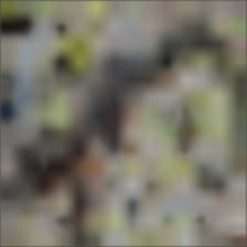
S1
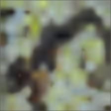
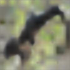
S2

Figure 7: The illustration showcases DIP visualizations for the lizard in ImageNet-A. The first row features images generated at each task period using embeddings from the ImageNet-21K pre-trained model. The second and third rows display images produced by embeddings from the Subnetwork-1 (S1) Adaptation Module and the Subnetwork-2 (S2) Adaptation Module.

	ViT-21K	S1 Task-0	S1 Task-9	S2 Task-0	S2 Task-9	Hybrid Task-0	Hybrid Task-9
ImageNet-R
ImageNet-A

Figure 8: The illustration of the t-SNE visualization for samples from Task 0 on the ImageNet-R and ImageNet-A datasets primarily focuses on the original ViT-21K pre-trained features. It also includes subnetwork-1 (S1) adaptation features, subnetwork-2 (S2) adaptation features, and hybrid adaptation features from weights at Task-0 and Task-9 stages, helping to elucidate the evolution and differentiation of feature representations across different stages.

TABLE VII: Performance analysis in NTK-CL for different pre-trained weights of ViT-B/16. The bolded segments represent the optimal results, while the underlined segments represent suboptimal results.

Method	CIFAR-100		ImageNet-R		ImageNet-A
	$\bar{A}$ (%)	$A_{T}$ (%)	$\bar{A}$ (%)	$A_{T}$ (%)	$\bar{A}$ (%)	$A_{T}$ (%)
Self-Supervised Methods
Dino ImageNet-1K [9]	84.85 $\pm$ 0.46	78.09 $\pm$ 0.44	74.08 $\pm$ 0.70	66.88 $\pm$ 0.35	45.03 $\pm$ 1.03	34.85 $\pm$ 0.82
MAE ImageNet-1K [23]	48.29 $\pm$ 3.80	41.59 $\pm$ 2.05	40.49 $\pm$ 1.33	32.73 $\pm$ 1.40	8.63 $\pm$ 1.54	5.66 $\pm$ 1.83
iBOT ImageNet-1K [101]	87.36 $\pm$ 0.53	81.78 $\pm$ 0.24	76.54 $\pm$ 0.88	69.52 $\pm$ 0.48	52.34 $\pm$ 1.39	42.40 $\pm$ 0.97
iBOT ImageNet-22K [101]	89.91 $\pm$ 0.44	84.76 $\pm$ 0.40	73.93 $\pm$ 0.65	65.37 $\pm$ 0.72	55.31 $\pm$ 1.91	44.42 $\pm$ 0.91
Supervised Methods
CLIP-Vision WIT [63]	82.71 $\pm$ 0.69	74.91 $\pm$ 0.52	84.17 $\pm$ 0.91	77.91 $\pm$ 0.56	61.42 $\pm$ 0.64	51.88 $\pm$ 1.08
MiiL ImageNet-1K [67]	88.84 $\pm$ 0.17	83.12 $\pm$ 1.02	78.83 $\pm$ 0.45	72.63 $\pm$ 0.60	62.12 $\pm$ 0.34	51.28 $\pm$ 0.57
SAM ImageNet-1K [17]	91.28 $\pm$ 0.47	86.50 $\pm$ 0.51	74.86 $\pm$ 0.68	68.29 $\pm$ 0.65	53.81 $\pm$ 0.57	44.69 $\pm$ 0.58
MiiL ImageNet-21K [67]	87.83 $\pm$ 0.39	82.37 $\pm$ 1.31	74.09 $\pm$ 0.48	66.29 $\pm$ 0.82	56.24 $\pm$ 0.62	44.85 $\pm$ 1.29
Supervised ImageNet-1K	93.16 $\pm$ 0.46	89.43 $\pm$ 0.34	83.18 $\pm$ 0.40	77.76 $\pm$ 0.25	68.76 $\pm$ 0.71	60.58 $\pm$ 0.56
Supervised ImageNet-21K	93.76 $\pm$ 0.35	90.27 $\pm$ 0.20	82.77 $\pm$ 0.66	77.17 $\pm$ 0.19	66.56 $\pm$ 1.53	58.54 $\pm$ 0.91

6.3 Hyper-parameters Adjustment

Next, we will experiment with variations of the hyper-parameters $\eta$, $\upsilon$, and $\lambda$ to explore the impact of $\mathcal{L}_{dis}$, $\mathcal{L}_{orth}$, and $\mathcal{L}_{reg}$ on PEFT-CL performance to varying degrees. All experiments use a fixed random seed of 0 to ensure fair comparison. The optimal hyper-parameter settings differ between datasets. For ImageNet-R, the optimal values are set at $\eta=0.2$, $\upsilon=0.0001$, and $\lambda=0.001$. Conversely, for CIFAR100, the optimal settings are $\eta=0.03$, $\upsilon=0.0001$, and $\lambda=0.001$. During these experiments, while one parameter is varied, the other hyper-parameters are held constant to isolate the effects of the variable under study. The detailed tuning experiments for these hyper-parameters on ImageNet-R and CIFAR100 are displayed in Fig. 5.

As illustrated in Fig. 5, variations in $\eta$, $\upsilon$, and $\lambda$ significantly impact the performance of the PEFT-CL model during continual training. Keeping the values for orthogonality and regularization tightly around 0.0001 and 0.001, respectively, is crucial. Deviations can lead to significant performance degradation for both current and previous tasks. This highlights the challenge that overly stringent orthogonality between task features and parameter regularization can undermine the model’s basic classification performance. How to balance these aspects and eliminate negative impacts is a key issue that needs to be addressed in future PEFT-CL research.

6.4 Visualisation

To visually demonstrate the information captured by the pre-trained ViT and processed through the Subnetwork-1 and Subnetwork-2 Adaptation Modules, we select a random image from Task 0. We extract three-dimensional embeddings using parameters from these modules at various training stages and employ the Deep Image Prior (DIP) technique [74] to reconstruct the image information based on these embeddings. The Hybrid Adaptation Module, which uses two-dimensional features from the CLS Token, does not support DIP reconstruction visualizations. However, the embeddings from the Subnetwork-1 and Subnetwork-2 Adaptation Modules, which serve as inputs to the Hybrid Adaptation Module, sufficiently illustrate the network’s learning and memory capabilities. This approach offers a clear visual representation of how each module processes and retains information across different tasks, highlighting the dynamic learning and generalization capabilities of the adaptation modules in our NTK-CL framework.

In Fig. 6 and Fig. 7, we provide a detailed display of the DIP visualization results for images from Task-0 on ImageNet-R and ImageNet-A. These visualizations reveal distinct differences in the information captured by the Subnetwork-1 and Subnetwork-2 Adaptation Modules. Specifically, the Subnetwork-2 Adaptation Module tends to focus more on the shapes and inherent features of the images, whereas the Subnetwork-1 Adaptation Module emphasizes color and fine details. This distinction underscores our design strategy of differentiating feature subspaces and provides optimal input for the Hybrid Adaptation Module. Additionally, the evolution from Task-0 to Task-9 within our NTK-CL framework demonstrates its capability to effectively retain knowledge from previous tasks, affirming the efficacy of our Knowledge Retention innovation in maintaining consistent performance across tasks. In any embedding space generated by our adaptation modules, the information is well-maintained and aligns closely with the original pre-trained knowledge.

To further elucidate the evolution and advantages of subnetwork-1 adaptation features, subnetwork-2 adaptation features, and hybrid adaptation features during continual training, we conduct detailed t-SNE experiments. Utilizing the original ViT-21K pre-trained weights as a baseline, we compare the features of samples from Task 0 at both Task-0 and Task-9 stages. As illustrated in Fig. 8, the subnetwork-1 adaptation features, subnetwork-2 adaptation features, and hybrid adaptation features all exhibit significantly enhanced discriminability compared to the features produced by the original ViT-21K pre-trained weights. Additionally, the discriminability of Task-0 samples is effectively maintained even at Task-9, which to a certain extent demonstrates the anti-forgetting capability of our framework. Notably, the hybrid adaptation features show superior discriminability relative to both subnetwork-1 adaptation features and subnetwork-2 adaptation features, affirming the effectiveness of the fusion component in our framework.

6.5 Other Pre-trained Weights

To more comprehensively explore the impact of $f_{0}^{*}$ in Eq. 3 on the final performance of PEFT-CL, extensive experiments using other pre-trained weights for ViT-B/16 are conducted. To ensure absolute fairness, the hyper-parameters and training strategies involved during their training are kept completely consistent, with only the backbone parameters differing. The results, as shown in Table VII, reveal several key insights.

Firstly, self-supervised methods exhibit significant variability, with iBOT ImageNet-22K [101] achieving the highest incremental accuracy on CIFAR-100 and ImageNet-A. This indicates a positive correlation between sample size, model generalizability, and resistance to forgetting, as articulated in lemma 3. In addition, the autoregressive self-supervised method MAE exhibits extreme disadvantages in both performance on individual tasks and resistance to forgetting. The reasons for this are not yet known, leaving room for further exploration.

Secondly, traditional supervised pre-trained weights, consistently demonstrate superior performance across all datasets, clearly outperforming other customized supervisory weights. This trend suggests that excessive pre-training strategies may not necessarily enhance model generalizability in PEFT-CL, despite their potential advantages under standard training paradigms. Furthermore, CLIP-Vision, which relies solely on visual information, only achieves state-of-the-art results on ImageNet-R. This outcome does not negate the value of more extensive sample sets. Instead, it implies that the dual-modal (Vision+Text) pre-training paradigm may not fully capitalize on the benefits of extensive training samples when employed solely within the visual modality.

These findings underscore the pivotal importance of choosing appropriate pre-training weights $f_{0}^{*}$ for optimizing PEFT-CL performance. They direct future research toward enhancing model robustness and generalization capabilities, crucial for dynamic learning environments.

7 Conclusion

In this study, we adopt an NTK perspective to analyze PEFT-CL tasks, elucidating model behavior and generalization gaps in sequential task learning. Our analysis identifies crucial factors affecting PEFT-CL effectiveness, particularly through the dynamics of task interplay and task-specific generalization gaps. We recommend strategies to mitigate these gaps, such as expanding sample sizes, enforcing task-level feature constraints, and refining regularization techniques. These strategies inform architectural and optimization adjustments aimed at enhancing the generalization capabilities and efficiency of PEFT-CL models across diverse tasks. This research significantly advances the theoretical framework and provides practical guidelines for improving PEFT-CL methodologies, contributing to both academic insights and real-world applications.

Jingren Liu received the B.S. degree in Computer Science and Technology from Nanjing University of Finance and Economy, Nanjing, China, in 2019, and is currently working toward the PhD degree in the School of Electrical and Information Engineering, Tianjin University, Tianjin, China. His current research interests include continual learning, few-shot learning, and prompt learning.

Zhong Ji received the Ph.D. degree in signal and information processing from Tianjin University, Tianjin, China, in 2008. He is currently a Professor with the School of Electrical and Information Engineering, Tianjin University. He has authored over 100 technical articles in refereed journals and proceedings. His current research interests include continual learning, few shot leanring, and cross-modal analysis.

YunLong Yu received the Ph.D. degree in information and communication engineering from Tianjin University, Tianjin, China, in 2019. He is currently a Distinguished Researcher with the College of Information Science and Electronic Engineering, Zhejiang University, Hangzhou, China. His current research interests include machine learning and computer vision.

Jiale Cao received the Ph.D degree in information and communication engineering from Tianjin University, Tianjin, China, in 2018. He is currently an Associate Professor with Tianjin University. His research interests include image understanding and analysis, in which he has published 30+ IEEE Transactions and CVPR/ICCV/ECCV articles. He serves as a regular Program Committee Member for leading computer vision and artificial intelligence conferences, such as CVPR, ICCV, and ECCV.

YanWei Pang received the Ph.D. degree in electronic engineering from the University of Science and Technology of China, Hefei, China, in 2004. He is currently a Professor with the School of Electrical and Information Engineering, Tianjin University, Tianjin, China. He has authored over 200 scientific papers. His current research interests include object detection and recognition, vision in bad weather, and computer vision.

Jungong Han received the Ph.D. degree in telecommunication and information system from Xidian University, Xi’an, China, in 2004. He is a Chair Professor of Computer Vision with the Department of Computer Science, University of Sheffield, U.K. He has published over 200 articles, including more than 80 IEEE Transactions and more than 50 A* conference articles. His research interests span the fields of video analysis, computer vision, and applied machine learning. He is a Fellow of the International Association of Pattern Recognition.

Xuelong Li is the Chief Technology Officer (CTO) and the Chief Scientist of the Institute of Artificial Intelligence (TeleAI) of China Telecom.

In the realm of PEFT-CL, we initiate with the foundational model $f_{0}^{*}$, where the superscript ^∗ signifies parameters optimized to their prime configuration, distinguishing them from those still under optimization. Our objective is to adeptly modify the feature space from $f_{0}^{*}$ for each specific task $i$ (represented as $f_{i}^{*}$), by finely adjusting the optimizable sub-network parameters $p_{i}$. This critical adaptation ensures that alterations in shared sub-network components across different tasks do not lead to excessive catastrophic forgetting, thereby safeguarding the model’s generalizability.

To methodically investigate PEFT-CL, we conceptualize a sequence of $T$ tasks, each optimizing sub-network parameters $p_{\tau}^{*}$ for $1\leq\tau\leq T$. This strategic adjustment of $p_{\tau}^{*}$ enables the model to achieve an optimal state $f_{\tau}^{*}$, thereby generating a specialized feature space for each task.

Expanding beyond traditional heuristic approaches [82, 81, 71, 36, 100] prevalent in PEFT-CL for adjusting sub-network components, our analysis delves into the training dynamics and explores the potential for reducing generalization gaps through the lens of NTK. This rigorous analysis helps pinpoint necessary adjustments to minimize generalization gaps and maximize model performance across diverse tasks. Grounded in seminal theories and contemporary studies in generalization dynamics [16, 10, 8, 37, 3], we introduce advanced tools for assessing task interplay and specific generalization gaps, as detailed in theorem 1 and theorem 2.

For comprehensive clarity in theoretical discourse, we segment our discussion into three distinct parts: analyzing NTK dynamics specific to PEFT-CL (Appendix A), evaluating inter-task generalization gap (Appendix B), and scrutinizing intra-task generalization gap (Appendix C). These segments collectively aim to provide a deep understanding of the underlying mechanisms influencing PEFT-CL performance, thereby informing better implementation practices in this field.

Appendix A NTK Dynamics in PEFT-CL

Initially, we concentrate on analyzing the least squares loss associated with the optimization of consecutive tasks $\tau$ and $\tau-1$. This involves quantifying the classification loss attributable to variations in the sub-network components’ parameters, which is expressed as follows:

$$\mathcal{L}(p_{\tau}|X,Y\in\mathcal{D_{\tau}})= \mathop{argmin}\limits_{p_{\tau}}\Bigl{\|}f_{\tau-1}^{*}(X)+\nabla_{p_{\tau}}f_{\tau}(X)$$ (31)

$$\times(p_{\tau}-p_{\tau-1}^{*})-Y\Bigr{\|}_{2}^{2},$$

$$= \mathop{argmin}\limits_{p_{\tau}}\Bigl{\|}f_{\tau-1}^{*}(X)+\phi_{\tau}(X)$$

$$\times(p_{\tau}-p_{\tau-1}^{*})-Y\Bigr{\|}_{2}^{2}.$$

Here, $D_{\tau}$ refers to the data subset associated with the $\tau$-th task, where $X$ and $Y$ are the input images and corresponding labels, respectively. The term $\phi_{\tau}(\cdot)$ denotes the Jacobian matrix relevant to task $\tau$ for the inputs $X$. At the onset of a task’s optimization, the sub-network component parameters inherit parameters from the preceding task, setting the initial states for optimizing $f_{\tau}(\cdot)$ and $p_{\tau}$ as $f_{\tau-1}^{*}(\cdot)$ and $p_{\tau-1}^{*}$, respectively.

To ensure a globally optimal solver $p_{\tau}^{*}$ for $p_{\tau}$ and a well-posed solution, we introduce an appropriate regularization term, transforming the initial loss defined in Eq. 31 to:

$$\mathcal{L}(p_{\tau}|X,Y \in\mathcal{D_{\tau}})=\mathop{argmin}\limits_{p_{\tau}}\left\|f_{\tau-1}^{*}(X)+\nabla_{p_{\tau}}f_{\tau}(X)\right.$$ (32)

$$\left.\times(p_{\tau}-p_{\tau-1}^{*})-Y\right\|_{2}^{2}+\lambda\left\|p_{\tau}-p_{\tau-1}^{*}\right\|_{2}^{2}.$$

The saddle-point solution of Eq. 32 is given by:

$$p_{\tau}-p_{\tau-1}^{*}=\phi_{\tau}(X)^{\top}(\phi_{\tau}(X)^{\top}\phi_{\tau}(X)+\lambda I)^{-1}(Y-f_{\tau-1}^{*}(X)).$$ (33)

Consequently, the optimal dynamic outputs for the $\tau$-th task during optimization can be expressed as:

$$f_{\tau}(x)= f_{\tau-1}^{*}(x)+\nabla_{p_{\tau}}f_{\tau}(x)(p_{\tau}-p_{\tau-1}^{*}),$$ (34)

$$= f_{\tau-1}^{*}(x)+\nabla_{p_{\tau}}f_{\tau}(x)\phi_{\tau}(X)^{\top}$$

$$\quad\times(\phi_{\tau}(X)^{\top}\phi_{\tau}(X)+\lambda I)^{-1}(Y-f_{\tau-1}^{*}(X)),$$

$$= f_{\tau-1}^{*}(x)+\phi_{\tau}(x)\phi_{\tau}(X)^{\top}$$

$$\quad\times(\phi_{\tau}(X)^{\top}\phi_{\tau}(X)+\lambda I)^{-1}(Y-f_{\tau-1}^{*}(X)),$$

$$= f_{\tau-1}^{*}(x)+\Phi_{\tau}(x,X)^{\top}$$

$$\quad\times(\Phi_{\tau}(X,X)+\lambda I)^{-1}(Y-f_{\tau-1}^{*}(X)).$$

Denoting $\tilde{Y}_{\tau}=Y-f_{\tau-1}^{*}(X)$, Equations 33 and 34 can be articulated as:

$$p_{\tau}-p_{\tau-1}^{*}=\phi_{\tau}(X)^{\top}(\Phi_{\tau}(X,X)+\lambda I)^{-1}\tilde{Y}_{\tau}.$$ (35)

$$f_{\tau}(x)-f_{\tau-1}^{*}(x)=\Phi_{\tau}(x,X)^{\top}(\Phi_{\tau}(X,X)+\lambda I)^{-1}\tilde{Y}_{\tau}.$$ (36)

Summing over Eq. 36, we obtain:

$$f_{\tau}(x)=f_{0}^{*}(x)+\sum\limits_{i=1}^{\tau}\Phi_{i}(x,X)(\Phi_{i}(X,X)+\lambda I)^{-1}\tilde{Y}_{i}.$$ (37)

Ultimately, when $f_{\tau}(\cdot)$ is optimized to the global optimum for task $\tau$, the NTK, derived from the gradients of $p_{\tau}$, is expected to converge and stabilize, preserving the forms of Equations 35, 36, and 37.

$$p_{\tau}^{*}-p_{\tau-1}^{*}=\phi_{\tau}(X)^{\top}(\Phi_{\tau}(X,X)+\lambda I)^{-1}\tilde{Y}_{\tau}.$$ (38)

$$f_{\tau}^{*}(x)-f_{\tau-1}^{*}(x)=\Phi_{\tau}(x,X)^{\top}(\Phi_{\tau}(X,X)+\lambda I)^{-1}\tilde{Y}_{\tau}.$$ (39)

$$f_{\tau}^{*}(x)=f_{0}^{*}(x)+\sum\limits_{i=1}^{\tau}\Phi_{i}(x,X)(\Phi_{i}(X,X)+\lambda I)^{-1}\tilde{Y}_{i}.$$ (40)

As delineated in Eq. 40, the output for task $\tau$ fundamentally hinges on the NTKs associated with the preceding $\tau$ tasks, the corresponding data labels, and the initial pre-trained weight.

Appendix B Task-Interplay Generalization in PEFT-CL

In this section, we explore the dynamics of task-interplay generalization gap within the PEFT-CL scenario, utilizing the NTK theory. We begin by outlining relevant mathematical properties of the NTK, followed by detailed analyses and derivations to elucidate how these properties influence generalization across tasks. This rigorous approach aims to provide a robust theoretical foundation for understanding the interplay between task transitions in PEFT-CL scenarios.

Owing to the reproducing property of the NTK function in the Reproducing Kernel Hilbert Space (RKHS), we deduce that for any task and any model, it follows that:

$$f(x)=\left<\Phi(\cdot,x),f\right>_{\mathcal{H}}.$$ (41)

In accordance with Mercer’s Theorem [55], within an ideal RKHS, the NTK can be expressed as an infinite sum of orthogonal basis functions and eigenvalues:

$$\Phi(x,x^{\prime})=\sum_{\rho}\lambda_{\rho}O_{\rho}(x)O_{\rho}(x^{\prime})=\sum_{\rho}\varphi_{\rho}(x)\varphi_{\rho}(x^{\prime}),|\rho|\rightarrow\infty,$$ (42)

where $\lambda$ and $O(\cdot)$ denote the eigenvalues and eigenfunctions from the decomposition, and $|\rho|$ signifies the count of eigenvalues and eigenfunctions realized post-decomposition. For clarity in subsequent derivations, we define $\varphi(\cdot)=\sqrt{\lambda}O(\cdot)$.

In addition, by denoting $\Phi_{\tau}(x,X)(\Phi_{\tau}(X,X)+\lambda I)^{-1}\tilde{Y}_{\tau}$ from Eq. 39 as $\alpha_{\tau}$, we deduce:

$$\tilde{f}^{*}_{\tau}(x)=\Phi_{\tau}(x,X)^{\top}\alpha_{\tau}=\sum\limits_{i=1}^{n_{t}}\Phi_{\tau}(x,x^{i})^{\top}\alpha_{\tau}^{i},$$ (43)

Here, $\tilde{f}$ denotes the functional difference between the outcomes of two consecutive tasks.

From the aforementioned content, it is known that in the RKHS, the norm of the function $\tilde{f}$ can be denoted as:

$$||\tilde{f}^{*}_{\tau}||^{2}_{\mathcal{H}}=\alpha_{\tau}^{\top}\Phi_{\tau}(X,X)\alpha_{\tau}.$$ (44)

Considering that $(\Phi_{\tau}(X,X)+\lambda I)^{-1}\leq(\Phi_{\tau}(X,X))^{-1}$ holds, we deduce the following inequality:

$$||\tilde{f}_{\tau}^{*}||^{2}_{\mathcal{H}} =\tilde{Y}_{\tau}^{\top}(\Phi_{\tau}(X,X)+\lambda I)^{-1}$$ (45)

$$\quad\times\Phi_{\tau}(X,X)(\Phi_{\tau}(X,X)+\lambda I)^{-1}\tilde{Y}_{\tau},$$

$$\leq\tilde{Y}_{\tau}^{\top}(\Phi_{\tau}(X,X)+\lambda I)^{-1}$$

$$\quad\times\Phi_{\tau}(X,X)(\Phi_{\tau}(X,X))^{-1}\tilde{Y}_{\tau},$$

$$\leq\tilde{Y}_{\tau}^{\top}(\Phi_{\tau}(X,X)+\lambda I)^{-1}\tilde{Y}_{\tau},$$

$$\leq G^{2}_{\tau}.$$

In relation to Equations 40, 43 and considering the symmetry properties of the inner product in high-dimensional Hilbert spaces, we can deconstruct it as:

$$f_{T}(x) =\sum\limits_{\tau=1}^{T}\sum\limits_{i=1}^{n_{\tau}}\alpha_{\tau}^{i}\left<\varphi_{\tau}(x),\varphi_{\tau}(x_{\tau}^{i})\right>_{\mathcal{H}},$$ (46)

$$=\sum\limits_{\tau=1}^{T}\sum\limits_{i=1}^{n_{\tau}}\alpha_{\tau}^{i}\left<\varphi_{\tau}(x_{\tau}^{i}),\varphi_{\tau}(x)\right>_{\mathcal{H}},$$

$$=\sum\limits_{\tau=1}^{T}\left<\sum\limits_{i=1}^{n_{\tau}}\alpha_{\tau}^{i}\varphi_{\tau}(x_{\tau}^{i}),\varphi_{\tau}(x)\right>_{\mathcal{H}},$$

Here, $\varphi_{\tau}(\cdot)$ denotes the matrix of orthogonal eigenfunctions and associated eigenvalues obtained from decomposing $\Phi_{\tau}(\cdot)$ in the RKHS for each task $\tau$. For this analysis, $f_{0}^{*}(x)$ is omitted, acting as a baseline constant in the model’s performance.

Considering the properties of Eq. 44, we infer:

$$||\sum\limits_{i=1}^{n_{\tau}}\alpha_{\tau}^{i}\varphi_{\tau}(x_{\tau}^{i})||_{\mathcal{H}}^{2} =\sum\limits_{i,j}\alpha_{\tau}^{i\top}\Phi_{\tau}(x_{\tau}^{i},x_{\tau}^{j})\alpha_{\tau}^{j}\leq G^{2}_{\tau},$$ (47)

$$\mathcal{F}_{T}\subset\{x\rightarrow\sum\limits_{\tau=1}^{T}\left<w_{\tau},\varphi_{\tau}(x)\right>_{\mathcal{H}},||w_{\tau}||_{\mathcal{H}}^{2}\leq G^{2}_{\tau}\}_{\mathcal{D}}:=\tilde{\mathcal{F}}_{T},$$ (48)

Initially, the set $\tilde{\mathcal{F}}_{T}$ comprises functions characterized by the inner product between the feature mapping $\varphi_{\tau}(x)$ and the weight vector $w_{\tau}$ within the RKHS, in the form of $\left<w_{\tau},\varphi_{\tau}(x)\right>_{\mathcal{H}}$. Accordingly, any arbitrary function $f_{\tau}^{*}(x)$ in $\mathcal{F}_{T}$ can be decomposed into the sum of the output of the previous task and the current task output change $f_{\tau}^{*}(x)=f_{\tau-1}^{*}(x)+\tilde{f}_{\tau}^{*}(x)$, and $\tilde{f}_{\tau}^{*}(x)$ is reconstructed into $\left<w_{\tau},\varphi_{\tau}(x)\right>_{\mathcal{H}}$. Thus, as every function $f_{\tau}^{*}(x)$ in $\mathcal{F}_{T}$ can be reconstructed into the form found in $\tilde{\mathcal{F}}_{T}$, it can be concluded that $\mathcal{F}_{T}$ is a subset of $\tilde{\mathcal{F}}_{T}$.

Combining the computation method of Rademacher Complexity, we obtain the upper bound of $\hat{\mathcal{R}}(\tilde{\mathcal{F}})$,

$$\hat{\mathcal{R}}(\mathcal{F}) =\mathbb{E}_{\epsilon}\left[\sup_{f\in\mathcal{F}}\frac{1}{n}\sum_{i=1}^{n}\epsilon_{i}f(x_{i})\right],$$ (49)

$$\hat{\mathcal{R}}(\mathcal{F}_{T}) \leq\hat{\mathcal{R}}(\tilde{\mathcal{F}}_{T}),$$

$$=\sum\limits_{\tau=1}^{T}\mathbb{E}_{\epsilon}\left[\sup_{||w_{\tau}||_{\mathcal{H}}^{2}\leq G_{\tau}^{2}}\left<w_{\tau},\frac{1}{n_{\tau}}\sum_{i=1}^{n_{\tau}}\epsilon_{i}\varphi_{\tau}(x_{\tau}^{i})\right>_{\mathcal{H}}\right],$$ (50)

where $\epsilon_{i}$ are independently and identically distributed random variables, taking values of $\pm 1$. And since $\mathcal{F}_{T}$ is a subset of $\tilde{\mathcal{F}}_{T}$, its Rademacher Complexity is less than or equal to that of $\tilde{\mathcal{F}}_{T}$.

Lemma 5.

Consider a kernel $k:\mathcal{X}\times\mathcal{X}\to\mathbb{R}$, and let $X_{1},\ldots,X_{n}$ be random elements of $\mathcal{X}$. Then for the class $\mathcal{F}$ defined above,

$$\hat{\mathcal{G}}_{n}(\mathcal{F}) \leq\frac{2B}{n}\sqrt{\sum_{i=1}^{n}\mathbb{E}[k(X_{i},X_{i})]},$$ (51)

$$\hat{\mathcal{R}}_{n}(\mathcal{F}) \leq\frac{2B}{n}\sqrt{\sum_{i=1}^{n}\mathbb{E}[k(X_{i},X_{i})]}.$$ (52)

Proof.

Suppose that $\mathcal{H}$ is a Hilbert space with inner product $\langle\cdot,\cdot\rangle$ and induced norm $\|\cdot\|$, and the kernel $k$ has feature map $\phi:\mathcal{X}\to\mathcal{H}$. Let $g_{1},\ldots,g_{n}$ be independent standard normal random variables. Then

$$\begin{split}\hat{\mathcal{G}}_{n}(\mathcal{F})&\leq\mathbb{E}\left[\sup_{\|w\|\leq B}\left<w,\frac{2}{n}\sum_{i=1}^{n}g_{i}\phi(X_{i})\right>_{\mathcal{H},\mathcal{D}}\right]\\ &=\frac{2B}{n}\mathbb{E}\left[\sqrt{\sum_{i=1}^{n}g_{i}^{2}\phi(X_{i})^{T}\phi(X_{i})}\right]\\ &=\frac{2B}{n}\mathbb{E}\left[\sqrt{\sum_{i,j}^{n}g_{i}g_{j}k(X_{i},X_{j})}\right]\\ &\leq\frac{2B}{n}\sqrt{\mathbb{E}\left[\sum_{i,j}^{n}g_{i}g_{j}k(X_{i},X_{j})\right]}\\ &=\frac{2B}{n}\sqrt{\sum_{i=1}^{n}\mathbb{E}[k(X_{i},X_{i})]}.\end{split}$$ (53)

Clearly, the same argument applies with any independent, zero mean, unit variance random variables replacing the $g_{i}$, which gives the same bound for $\hat{\mathcal{R}}_{n}(\mathcal{F})$.

From the definitions and Jensen’s inequality, we can deduce that:

$$R_{n}(\mathcal{F}) =\mathbb{E}R_{n}(\mathcal{F})\leq 2B\sqrt{\frac{\mathbb{E}k(X,X)}{n}},$$ (54)

$$G_{n}(\mathcal{F}) =\mathbb{E}\hat{G}_{n}(\mathcal{F})\leq 2B\sqrt{\frac{\mathbb{E}k(X,X)}{n}}.$$ (55)

It is noteworthy that $\mathbb{E}k(X,X)$ represents the trace (sum of the eigenvalues) of the integral operator $T_{k}$ defined on $L_{2}(\mu)$,

$$T_{k}(f)=\int k(x,y)f(y)d\mu(y),$$ (56)

where $\mu$ is the induced probability measure on $\mathcal{X}$. ∎

Utilizing the lemma 5 from [2], we can derive:

$$\hat{\mathcal{R}}(\mathcal{F}_{T}) \leq\left[\sum\limits_{\tau=1}^{T}\frac{G_{\tau}}{n_{\tau}}\sqrt{\text{Tr}(\Phi_{\tau}(X,X))}\right]_{\mathcal{D}_{\tau}},$$ (57)

$$=\left[\sum\limits_{\tau=1}^{T}\sqrt{\frac{[\tilde{Y}_{\tau}^{\top}(\Phi_{\tau}(X,X)+\lambda I)^{-1}\tilde{Y}_{\tau}]\text{Tr}(\Phi_{\tau}(X,X))}{n_{\tau}^{2}}}\right]_{\mathcal{D}_{\tau}},$$

$$=\left[\sum\limits_{\tau=1}^{T}\mathcal{O}(\sqrt{\frac{[\tilde{Y}_{\tau}^{\top}(\Phi_{\tau}(X,X)+\lambda I)^{-1}\tilde{Y}_{\tau}]}{n_{\tau}}})\right]_{\mathcal{D}_{\tau}}.$$

Expanding upon Eq. 39, we express the generalization dynamics of PEFT-CL for the final task as follows:

$$f_{T}^{*}(x)=f^{*}_{\tau}(x)+\sum\limits_{k=\tau+1}^{T}\tilde{f}^{*}_{k}(x),$$ (58)

$$||f_{T}^{*}(X_{\tau})-Y_{\tau}||_{2}^{2} =||f^{*}_{\tau}(X_{\tau})+\sum\limits_{k=\tau+1}^{T}\tilde{f}^{*}_{k}(X_{\tau})-Y_{\tau}||_{2}^{2},$$ (59)

$$\leq||f^{*}_{\tau}(X_{\tau})-Y_{\tau}||_{2}^{2}+\sum\limits_{k=\tau+1}^{T}||\tilde{f}^{*}_{k}(X_{\tau})||_{2}^{2}.$$

For the first term on the right-hand side of Eq. 59, we derive the following inequality:

$$||f^{*}_{\tau}(X_{\tau})-Y_{\tau}||_{2}^{2} =||\tilde{f}^{*}_{\tau}(X_{\tau})+f^{*}_{\tau-1}(X_{\tau})-Y_{\tau}||_{2}^{2},$$ (60)

$$=||\tilde{f}^{*}_{\tau}(X_{\tau})-\tilde{Y}_{\tau}||_{2}^{2},$$

$$=||\Phi_{\tau}(X_{\tau},X_{\tau})^{\top}(\Phi_{\tau}(X_{\tau},X_{\tau})+\lambda I)^{-1}$$

$$\quad\times\tilde{Y}_{\tau}-\tilde{Y}_{\tau}||_{2}^{2},$$

$$=||[\Phi_{\tau}(X_{\tau},X_{\tau})+\lambda I-\lambda I]^{\top}$$

$$\quad\times(\Phi_{\tau}(X_{\tau},X_{\tau})+\lambda I)^{-1}\tilde{Y}_{\tau}-\tilde{Y}_{\tau}||_{2}^{2},$$

$$=||\tilde{Y}_{\tau}-\lambda(\Phi_{\tau}(X_{\tau},X_{\tau})+\lambda I)^{-1}$$

$$\quad\times\tilde{Y}_{\tau}-\tilde{Y}_{\tau}||_{2}^{2},$$

$$=\lambda^{2}||(\Phi_{\tau}(X_{\tau},X_{\tau})+\lambda I)^{-1}$$

$$\quad\times\tilde{Y}_{\tau}||_{2}^{2},$$

$$\leq\lambda^{2}\tilde{Y}_{\tau}^{\top}(\Phi_{\tau}(X_{\tau},X_{\tau})+\lambda I)^{-1}\tilde{Y}_{\tau}.$$

Utilizing the formulation in Eq. 39, we further deduce:

$$||\tilde{f}^{*}_{k}(X_{\tau})||_{2}^{2}= \tilde{Y}_{k}^{\top}(\Phi_{k}(X_{k},X_{k})+\lambda I)^{-1}\Phi_{k}(X_{\tau},X_{k})$$ (61)

$$\times\Phi_{k}(X_{\tau},X_{k})^{\top}(\Phi_{k}(X_{k},X_{k})+\lambda I)^{-1}\tilde{Y}_{k}.$$

Then, the inequality for $||f_{T}^{*}(X_{\tau})-Y_{\tau}||_{2}^{2}$ is given by:

$$\mathcal{L}_{S}(f_{T}^{*}) =||f_{T}^{*}(X_{\tau})-Y_{\tau}||_{2}^{2}$$ (62)

$$\leq\frac{1}{n_{\tau}}\Big{[}\lambda^{2}\tilde{Y}_{\tau}^{\top}(\Phi_{\tau}(X_{\tau},X_{\tau})+\lambda I)^{-1}\tilde{Y}_{\tau}$$

$$+\sum\limits_{k=\tau+1}^{T}\tilde{Y}_{k}^{\top}(\Phi_{k}(X_{k},X_{k})+\lambda I)^{-1}$$

$$\quad\times\Phi_{k}(X_{\tau},X_{k})\Phi_{k}(X_{\tau},X_{k})^{\top}$$

$$\quad\times(\Phi_{k}(X_{k},X_{k})+\lambda I)^{-1}\tilde{Y}_{k}\Big{]}.$$

Building upon the insights of [2], we can assert that, with probability at least $1-\delta$, the disparity between the population loss $L_{D}(f)$ and the empirical loss $L_{S}(f)$ for any function $f$ within the function class $\mathcal{F}_{T}$ is bounded as follows:

$$\sup_{f\in\mathcal{F}_{T}}\{L_{D}(f)-L_{S}(f)\}\leq 2\rho\hat{\mathcal{R}}(\mathcal{F}_{T})+3c\sqrt{\frac{\log(2/\delta)}{2N}},$$ (63)

Furthermore, applying this principle to our optimal function $f^{*}_{T}$ from $\mathcal{F}_{T}$, we obtain an upper bound for the population loss $L_{D}(f^{*}_{T})$ in terms of the empirical loss $L_{S}(f^{*}_{T})$, as delineated below:

$$L_{D}(f^{*}_{T})\leq L_{S}(f^{*}_{T})+2\rho\hat{\mathcal{R}}(\mathcal{F}_{T})+3c\sqrt{\frac{\log(2/\delta)}{2N}},$$ (64)

Here, $\rho$ represents the Lipschitz constant. The term $\hat{\mathcal{R}}(\mathcal{F}_{T})$ refers to the empirical Rademacher complexity, as detailed in Eq. 57. $L_{S}(f^{*}_{T})$ represents the empirical loss in Eq. 62 and $\delta$ specifies the confidence level. While $c$ is a constant and $N$ denotes the total sample size.

Appendix C Task-Intrinsic Generalization in PEFT-CL

Utilizing Eq. 40 and momentarily setting aside the initialization term $f_{0}^{*}(x)$, we identify the NTK-related term for the entire task dataset as $\alpha_{i}$. Incorporating its eigen-decomposition, we derive:

$$f_{\tau}^{*}(x) =\sum_{i=1}^{\tau}\alpha_{i}\sum_{\rho}\lambda_{\rho}O_{\rho}(x)O_{\rho}(X)$$ (65)

$$=\sum_{\rho}\left(\sum_{i=1}^{\tau}\alpha_{i}\varphi_{\rho}(X)\right)\varphi_{\rho}(x).$$

Defining $w_{\rho}=\sum\limits_{i=1}^{\tau}\alpha_{i}\varphi_{\rho}(X)$, the function $f_{\tau}^{*}(x)$ is representable as $f_{\tau}^{*}(x)=\sum\limits_{\rho}w_{\rho}\varphi_{\rho}(x)$. Consequently, under any task scenario, its output can be decomposed into a linear combination of eigenvalues and orthogonal eigenfunctions in the RKHS.

At this juncture, within the task, the generalization gap can be expressed as:

$$\mathbb{E}_{g}(f_{\tau},f_{\tau}^{*}) =\left<(f_{\tau}(x)-y_{\tau}(x))^{2}\right>_{x\in D_{\tau}}$$ (66)

$$=\sum_{\rho,\gamma}(w_{\rho}-w_{\rho}^{*})(w_{\gamma}-w_{\gamma}^{*})\left<\varphi_{\rho}(x),\varphi_{\gamma}(x)\right>_{x\in D_{\tau}}.$$

Given that $\varphi_{\rho}(x)$ and $\varphi_{\gamma}(x)$ form the inner product of the Dirac function $\delta$ in RKHS, Eq. 66 is transformed into:

$$\mathbb{E}_{g}(f_{\tau},f_{\tau}^{*}) =\sum_{\rho}\lambda_{\rho}\left<(w_{\rho}-w_{\rho}^{*})^{2}\right>_{x\in D_{\tau}},$$ (67)

$$=(w-w^{*})\Lambda(w-w^{*}),$$

where $\Lambda=\lambda_{\rho}\delta_{\rho\gamma},\rho=\gamma$. Here, $w$ and $w^{*}$ denote matrices composed of weights corresponding to the orthogonal eigenfunctions reconstituted in the RKHS for each output.

In an approach analogous to the solution process for NTK Dynamics discussed in Appendix A, we construct a kernel regression error for the weight matrix $w$:

$$\mathbb{E}_{w}=||\varphi(x)^{\top}w-y||_{2}^{2}+\lambda||w||_{2}^{2},$$ (68)

where $\varphi(x)$ represents the matrix composed of $\varphi_{\rho}(x_{i})$. For simplicity, we omit the subscript in a similar manner to the treatment of $w$.

By obtaining the saddle-point solution that minimizes the kernel regression error, we arrive at:

$$w =(\varphi(x)\varphi(x)^{\top}+\lambda I)^{-1}\varphi(x)y,$$ (69)

$$=(\varphi(x)\varphi(x)^{\top}+\lambda I)^{-1}\varphi(x)\varphi(x)^{\top}w^{*},$$

$$=(\varphi(x)\varphi(x)^{\top}+\lambda I)^{-1}[(\varphi(x)\varphi(x)^{\top}+\lambda I)w^{*}-\lambda w^{*}],$$

$$=w^{*}-\lambda(\varphi(x)\varphi(x)^{\top}+\lambda I)^{-1}w^{*}.$$

Substituting $w-w^{*}=-\lambda(\varphi(x)\varphi(x)^{\top}+\lambda I)^{-1}w^{*}$ back into Eq. 67, we obtain:

$$\mathbb{E}_{g}(f_{\tau},f_{\tau}^{*})=\lambda^{2}\Big{<}w^{*}(\varphi(x)\varphi(x)^{\top}+\lambda I)^{-1}$$ (70)

$$\times\Lambda(\varphi(x)\varphi(x)^{\top}+\lambda I)^{-1}w^{*}\Big{>}_{x\in D_{\tau}}.$$

As both $\Lambda$ and $w^{*}$ are diagonal matrices, we separate them from the non-diagonal matrix part for easier solving:

$$\mathbb{E}_{g}(f_{\tau},f_{\tau}^{*}) =\lambda^{2}\left<w^{*}(\varphi(x)\varphi(x)^{\top}+\lambda I)^{-1}\right.$$ (71)

$$\quad\left.\times\Lambda(\varphi(x)\varphi(x)^{\top}+\lambda I)^{-1}w^{*}\right>_{x\in D_{\tau}},$$

$$=\left<\Lambda^{-\frac{1}{2}}w^{*}w^{*\top}\Lambda^{-\frac{1}{2}}\right>_{x\in D_{\tau}}$$

$$\quad\times\left<(\lambda\Lambda^{\frac{1}{2}}(\varphi(x)\varphi(x)^{\top}+\lambda I)^{-1}\Lambda^{\frac{1}{2}})^{2}\right>_{x\in D_{\tau}},$$

$$=\left<\Lambda^{-\frac{1}{2}}w^{*}w^{*\top}\Lambda^{-\frac{1}{2}}\right>_{x\in D_{\tau}}$$

$$\quad\times\left<((\frac{1}{\lambda}O(x)O(x)^{\top}+\Lambda^{-1})^{-1})^{2}\right>_{x\in D_{\tau}},$$

$$=\sum_{\rho}\sum_{\gamma}\left<K_{\rho,\gamma}U^{2}_{\rho,\gamma}\right>_{x\in D_{\tau}}.$$

Drawing from [72] and [10], we aim to determine the dynamic changes of $U_{\rho,\gamma}$. Introducing auxiliary variable $z$ and data quantity variable $s$, $U_{\rho,\gamma}$ can be represented as:

$$U_{\rho,\gamma}(s,z)=\left(\frac{1}{\lambda}O(x)O(x)^{\top}+\Lambda^{-1}+zI\right)^{-1}.$$ (72)

At this stage of the analysis, by applying the Woodbury Matrix Inversion Formula [70], we derive the following expression:

$$\left<U(s+1,z)\right>_{x\in D_{\tau}}=\left<\left(U(s,z)^{-1}+\frac{1}{\lambda}O(x)O(x)^{\top}\right)^{-1}\right>_{x\in D_{\tau}},$$ (73)

$$=\left<U(s,z)\right>_{x\in D_{\tau}}-\left<U(s,z)O(x)\right>_{x\in D_{\tau}}$$

$$\quad+\left<(\lambda I+O(x)^{\top}U(s,z)O(x))^{-1}O(x)^{\top}U(s,z)\right>_{x\in D_{\tau}},$$

$$=\left<U(s,z)\right>_{x\in D_{\tau}}-\left<\frac{U(s,z)O(x)O(x)^{\top}U(s,z)}{\lambda+O(x)^{\top}U(s,z)O(x)}\right>_{x\in D_{\tau}},$$

For the sake of conciseness, we continue to omit the subscripts $\rho$ and $\gamma$ in this proof.

Confronted with the intricate condition of averaging the last term on the right-hand side, we employ an approximation method where the numerator and denominator are averaged separately. This leads to the ensuing approximation:

$$\left<U(s+1,z)\right>_{x\in D_{\tau}}\approx\left<U(s,z)\right>_{x\in D_{\tau}}-\frac{\left<U(s,z)^{2}\right>_{x\in D_{\tau}}}{\lambda+\text{Tr}\left<U(s,z)\right>_{x\in D_{\tau}}}.$$ (74)

Considering $s$ as a continuous variable, we derive the first-order dynamics of $U$ with respect to $s$:

$$\nabla U(s,z)|_{s}=U(s+1,z)-U(s,z)\approx-\frac{\left<U(s,z)^{2}\right>}{\lambda+\text{Tr}\left<U(s,z)\right>}.$$ (75)

Next, revisiting Equations 71 and 72, by taking the first-order derivative with respect to variable $z$ and setting it to zero, we arrive at:

$$\nabla U(s,z)|_{z=0}=-(\frac{1}{\lambda}O(x)O(x)^{\top}+\Lambda^{-1})^{-2}=-U^{2}_{\rho,\gamma}.$$ (76)

Subsequently, by substituting Eq. 76 into Eq. 75, we deduce:

$$\nabla U(s,z)|_{s}\approx\frac{1}{\lambda+\text{Tr}\left<U(s,z)\right>}\nabla U(s,z)|_{z=0}.$$ (77)

To simplify subsequent derivations, we omit variables $s$ and $z$ from $U(s,z)$, yielding the following simplified expression:

$$\frac{\partial U}{\partial s}\approx\frac{1}{\lambda+\text{Tr}\left<U\right>}\frac{\partial U}{\partial z}.$$ (78)

For the given partial differential equation (PDE) in Eq. 78, we use the method of characteristics to solve it. This approach transforms the PDE into a set of ordinary differential equations (ODEs), describing the solution’s behavior along characteristic curves. These curves are paths in the solution space along which the PDE simplifies to an ODE. For path construction, we identify the normal vector $(-1,\frac{\partial U}{\partial s},\frac{\partial U}{\partial z})$, perpendicular to the vector $(0,1,-\frac{1}{\lambda+\text{Tr}\left<U\right>})$ in the PDE. From PDE in Eq. 78, we obtain a set of ODEs:

$$\frac{dU}{dv}=0,\quad\frac{ds}{dv}=1,\quad\frac{dz}{dv}=-\frac{1}{\lambda+\text{Tr}\left<U\right>},$$ (79)

$v$ is an additional variable we introduce, related to the characteristic curves.

Consequently, it can be deduced that $U$ is a constant term independent of $v$, with $s=v+s_{0}$ and $z=-\frac{v}{\lambda+\text{Tr}\left<U\right>}+z_{0}$. Since $s_{0}=0$ and in conjunction with Eq. 72, we obtain $U(s,z)=\left(\mathbf{\Lambda}^{-1}+z_{0}\mathbf{I}\right)^{-1}=\left(\mathbf{\Lambda}^{-1}+(z+\frac{v}{\lambda+\text{Tr}\left<U\right>})\mathbf{I}\right)^{-1}=\left(\mathbf{\Lambda}^{-1}+(z+\frac{s}{\lambda+\text{Tr}\left<U\right>})\mathbf{I}\right)^{-1}$.

Consequently, taking into account the properties of the Dirac function, we deduce the following equations:

$$U_{\rho,\gamma}(s,z)=\left(\frac{1}{\lambda_{\rho}}+z+\frac{s}{\lambda+\text{Tr}\left<U_{\rho,\gamma}(s,z)\right>}\right)^{-1},$$ (80)

$$TU(s,z) =\text{Tr}\left<U_{\rho,\gamma}(s,z)\right>$$ (81)

$$=\text{Tr}\left(\frac{1}{\lambda_{\rho}}+z+\frac{s}{\lambda+TU(s,z)}\right)^{-1},$$

$$\frac{\partial U_{\rho,\gamma}(s,z)}{\partial z}\bigg{|}_{z=0}= -\left(\frac{1}{\lambda_{\rho}}+\frac{s}{\lambda+TU(s,0)}\right)^{-2}$$ (82)

$$\times\left(1-\frac{s}{(\lambda+TU(s,0))^{2}}\frac{\partial TU(s,0)}{\partial z}\right).$$

Furthermore, since $U(s,z)$ at initialization is $U(0,z)=(\Lambda^{-1}+z\mathbf{I})^{-1}$, a diagonal matrix, and as the amount of data $s$ increases, $\frac{1}{\lambda}O(x)O(x)^{\top}$ will not change this diagonal property. Therefore, the derivative of its trace is equal to the sum of the derivatives of the original matrix.

$$\frac{\partial TU(s,z)}{\partial z}\bigg{|}_{z=0} =\sum\limits_{\rho}\frac{\partial U_{\rho,\gamma}(s,z)}{\partial z}\bigg{|}_{z=0},$$ (83)

$$=-\sum\limits_{\rho}\left(\frac{1}{\lambda_{\rho}}+\frac{s}{\lambda+TU(s,0)}\right)^{-2}$$

$$\quad\times\left(1-\frac{s}{(\lambda+TU(s,0))^{2}}\frac{\partial TU(s,0)}{\partial z}\right).$$

From the above formula derivation, we can conclude:

$$\frac{\partial TU(s,0)}{\partial z}=\frac{m}{\frac{ms}{(\lambda+TU(s,0))^{2}}-1}.$$ (84)

$$\frac{\partial U_{\rho,\gamma}(s,z)}{\partial z}= -\left(\frac{1}{\lambda_{\rho}}+\frac{s}{\lambda+TU(s,0)}\right)^{-2}$$ (85)

$$\times(1-\frac{ms}{(\lambda+TU(s,0))^{2}})^{-1}.$$

where $m=\sum\limits_{\rho}\left(\frac{1}{\lambda_{\rho}}+\frac{s}{\lambda+TU(s,0)}\right)^{-2}$.

Therefore, combining Eq. 72, the final generalization gap in this task can be represented as:

$$\mathbb{E}_{g} =\sum\limits_{\rho,\gamma}K_{\rho,\gamma}U^{2}_{\rho,\gamma}=-\sum\limits_{\rho}\frac{w_{\rho}^{*2}}{\lambda_{\rho}}\frac{\partial U_{\rho}(s,z)}{\partial z}\bigg{|}_{z=0},$$ (86)

$$=\sum\limits_{\rho}\frac{w_{\rho}^{*2}}{\lambda_{\rho}}\left(\frac{1}{\lambda_{\rho}}+\frac{s}{\lambda+TU(s,0)}\right)^{-2}$$

$$\quad\times(1-\frac{ms}{(\lambda+TU(s,0))^{2}})^{-1},$$

$$=\sum\limits_{\rho}\frac{w_{\rho}^{*2}}{\lambda_{\rho}}\left(\frac{1}{\lambda_{\rho}}+\frac{s}{\lambda+TU(s)}\right)^{-2}$$

$$\quad\times(1-\frac{ms}{(\lambda+TU(s))^{2}})^{-1}.$$

Further, it finally can be transformed into

$$\mathbb{E}_{g}=\sum\limits_{\rho,i}\frac{w_{\rho}^{*2}}{\lambda_{\rho}}\left(\frac{1}{\lambda_{\rho}}+\frac{s_{i}}{\lambda+tu_{i}}\right)^{-2}(1-\frac{m_{i}s_{i}}{(\lambda+tu_{i})^{2}})^{-1},$$ (87)

Here, the variable $s_{i}$ indicates the sample size for $i=1,2,\ldots,n_{\tau}$. The parameters $m_{i}$ and $tu_{i}$ are derived from the established relationships:

$$\small m_{i}=\sum_{\rho,i}(\frac{1}{\lambda_{\rho}}+\frac{s_{i}}{\lambda+m_{i}})^{-1},\quad tu_{i}=\sum_{\rho,i}(\frac{1}{\lambda_{\rho}}+\frac{s_{i}}{\lambda+m_{i}})^{-2}.$$ (88)

Appendix D Task Segmentation

In Tables VIII and IX, we outline the class order for CIFAR100, ImageNet-R, and ImageNet-A for each seed configuration. All subsequent task segmentations adhere to these class orders. The method to establish this class order involves setting the random seed and executing a random permutation of the class indices during task segmentation definition. The following code snippet illustrates this process:

All remaining datasets are divided in this manner to maintain consistency and replicability across experiments.

TABLE VIII: The class order for each seed on CIFAR100 determines all subsequent task segmentations.

Seed	Class Order
seed0	[26, 86, 2, 55, 75, 93, 16, 73, 54, 95, 53, 92, 78, 13, 7, 30, 22, 24, 33, 8, 43, 62, 3, 71, 45, 48, 6, 99, 82, 76, 60, 80, 90, 68, 51, 27, 18, 56, 63, 74, 1, 61, 42, 41, 4, 15, 17, 40, 38, 5, 91, 59, 0, 34, 28, 50, 11, 35, 23, 52, 10, 31, 66, 57, 79, 85, 32, 84, 14, 89, 19, 29, 49, 97, 98, 69, 20, 94, 72, 77, 25, 37, 81, 46, 39, 65, 58, 12, 88, 70, 87, 36, 21, 83, 9, 96, 67, 64, 47, 44]
seed1	[80, 84, 33, 81, 93, 17, 36, 82, 69, 65, 92, 39, 56, 52, 51, 32, 31, 44, 78, 10, 2, 73, 97, 62, 19, 35, 94, 27, 46, 38, 67, 99, 54, 95, 88, 40, 48, 59, 23, 34, 86, 53, 77, 15, 83, 41, 45, 91, 26, 98, 43, 55, 24, 4, 58, 49, 21, 87, 3, 74, 30, 66, 70, 42, 47, 89, 8, 60, 0, 90, 57, 22, 61, 63, 7, 96, 13, 68, 85, 14, 29, 28, 11, 18, 20, 50, 25, 6, 71, 76, 1, 16, 64, 79, 5, 75, 9, 72, 12, 37]
seed2	[83, 30, 56, 24, 16, 23, 2, 27, 28, 13, 99, 92, 76, 14, 0, 21, 3, 29, 61, 79, 35, 11, 84, 44, 73, 5, 25, 77, 74, 62, 65, 1, 18, 48, 36, 78, 6, 89, 91, 10, 12, 53, 87, 54, 95, 32, 19, 26, 60, 55, 9, 96, 17, 59, 57, 41, 64, 45, 97, 8, 71, 94, 90, 98, 86, 80, 50, 52, 66, 88, 70, 46, 68, 69, 81, 58, 33, 38, 51, 42, 4, 67, 39, 37, 20, 31, 63, 47, 85, 93, 49, 34, 7, 75, 82, 43, 22, 72, 15, 40]
seed3	[93, 67, 6, 64, 96, 83, 98, 42, 25, 15, 77, 9, 71, 97, 34, 75, 82, 23, 59, 45, 73, 12, 8, 4, 79, 86, 17, 65, 47, 50, 30, 5, 13, 31, 88, 11, 58, 85, 32, 40, 16, 27, 35, 36, 92, 90, 78, 76, 68, 46, 53, 70, 80, 61, 18, 91, 57, 95, 54, 55, 28, 52, 84, 89, 49, 87, 37, 48, 33, 43, 7, 62, 99, 29, 69, 51, 1, 60, 63, 2, 66, 22, 81, 26, 14, 39, 44, 20, 38, 94, 10, 41, 74, 19, 21, 0, 72, 56, 3, 24]
seed4	[20, 10, 96, 16, 63, 24, 53, 97, 41, 47, 43, 2, 95, 26, 13, 37, 14, 29, 35, 54, 80, 4, 81, 76, 85, 60, 5, 70, 71, 19, 65, 62, 27, 75, 61, 78, 18, 88, 7, 39, 6, 77, 11, 59, 22, 94, 23, 12, 92, 25, 83, 48, 17, 68, 31, 34, 15, 51, 86, 82, 28, 64, 67, 33, 45, 42, 40, 32, 91, 74, 49, 8, 30, 99, 66, 56, 84, 73, 79, 21, 89, 0, 3, 52, 38, 44, 93, 36, 57, 90, 98, 58, 9, 50, 72, 87, 1, 69, 55, 46]

TABLE IX: The class order for each seed on ImageNet-A and ImageNet-R determines all subsequent task segmentations.

Seed	Class Order
seed0	[18, 170, 107, 98, 177, 182, 5, 146, 12, 152, 61, 125, 180, 154, 80, 7, 33, 130, 37, 74, 183, 145, 45, 159, 60, 123, 179, 185, 122, 44, 16, 55, 150, 111, 22, 189, 129, 4, 83, 106, 134, 66, 26, 113, 168, 63, 8, 75, 118, 143, 71, 124, 184, 97, 149, 24, 30, 160, 40, 56, 131, 96, 181, 19, 153, 92, 54, 163, 51, 86, 139, 90, 137, 101, 144, 89, 109, 14, 27, 141, 187, 46, 138, 195, 108, 62, 2, 59, 136, 197, 43, 10, 194, 73, 196, 178, 175, 126, 93, 112, 158, 191, 50, 0, 94, 110, 95, 64, 167, 41, 69, 49, 48, 85, 13, 161, 23, 186, 135, 20, 15, 78, 104, 52, 100, 76, 3, 116, 164, 198, 6, 68, 84, 121, 155, 171, 156, 91, 199, 11, 119, 102, 35, 57, 65, 1, 120, 162, 42, 105, 132, 173, 17, 38, 133, 53, 157, 128, 34, 28, 114, 151, 31, 166, 127, 176, 32, 142, 169, 147, 29, 99, 82, 79, 115, 148, 193, 72, 77, 25, 165, 81, 188, 174, 190, 39, 58, 140, 88, 70, 87, 36, 21, 9, 103, 67, 192, 117, 47, 172]
seed1	[58, 40, 34, 102, 184, 198, 95, 4, 29, 168, 171, 18, 11, 89, 110, 118, 159, 35, 136, 59, 51, 16, 44, 94, 31, 162, 38, 28, 193, 27, 47, 165, 194, 177, 176, 97, 174, 73, 69, 172, 108, 107, 189, 14, 56, 19, 114, 39, 185, 124, 98, 123, 119, 53, 33, 179, 181, 106, 199, 138, 116, 67, 78, 42, 17, 5, 127, 105, 48, 66, 54, 84, 183, 158, 166, 113, 12, 117, 93, 120, 154, 90, 81, 122, 191, 13, 82, 132, 187, 45, 99, 36, 161, 186, 153, 103, 195, 197, 148, 173, 75, 21, 91, 152, 2, 70, 85, 150, 6, 112, 0, 155, 77, 65, 55, 167, 88, 130, 46, 62, 74, 92, 147, 160, 143, 87, 180, 145, 164, 10, 32, 83, 182, 100, 125, 23, 126, 9, 170, 104, 151, 135, 111, 188, 64, 15, 41, 163, 109, 80, 52, 26, 76, 43, 24, 3, 169, 49, 149, 131, 190, 30, 121, 115, 175, 8, 60, 128, 1, 57, 22, 61, 63, 7, 196, 141, 86, 96, 68, 50, 142, 157, 156, 139, 146, 101, 20, 178, 25, 134, 71, 129, 144, 192, 79, 133, 137, 72, 140, 37]
seed2	[112, 29, 182, 199, 193, 85, 10, 54, 115, 35, 12, 92, 13, 126, 174, 2, 44, 3, 113, 14, 23, 25, 6, 134, 165, 173, 45, 65, 48, 122, 178, 64, 9, 57, 78, 71, 128, 176, 131, 53, 137, 163, 111, 123, 109, 141, 41, 130, 140, 5, 159, 100, 11, 187, 24, 89, 66, 8, 172, 175, 28, 133, 94, 42, 169, 82, 184, 106, 108, 143, 180, 166, 146, 79, 1, 119, 192, 149, 160, 188, 147, 36, 171, 179, 62, 0, 27, 157, 98, 118, 20, 158, 156, 142, 77, 30, 154, 17, 59, 181, 114, 127, 139, 191, 93, 151, 21, 55, 16, 152, 91, 99, 120, 197, 74, 190, 161, 144, 196, 87, 90, 84, 18, 97, 101, 125, 164, 135, 61, 81, 68, 129, 56, 19, 86, 70, 60, 34, 40, 138, 76, 153, 26, 32, 195, 96, 83, 110, 105, 73, 117, 150, 145, 155, 198, 136, 39, 49, 186, 132, 50, 52, 80, 185, 121, 189, 46, 88, 69, 67, 183, 58, 33, 38, 103, 51, 107, 170, 4, 102, 167, 37, 116, 124, 148, 31, 63, 47, 194, 95, 177, 162, 7, 104, 75, 43, 22, 72, 15, 168]
seed3	[40, 51, 139, 197, 170, 82, 183, 46, 70, 100, 179, 83, 25, 190, 159, 173, 95, 3, 41, 58, 14, 143, 12, 6, 182, 161, 128, 122, 101, 86, 64, 47, 158, 34, 38, 196, 4, 72, 67, 145, 156, 115, 155, 15, 61, 175, 120, 130, 23, 153, 31, 103, 89, 132, 109, 126, 17, 30, 178, 162, 77, 73, 71, 78, 42, 133, 192, 13, 146, 74, 5, 114, 102, 181, 121, 168, 171, 24, 144, 92, 8, 53, 27, 105, 118, 163, 43, 57, 165, 22, 180, 187, 160, 87, 134, 63, 140, 193, 135, 45, 35, 65, 50, 125, 98, 16, 19, 108, 44, 68, 76, 141, 112, 10, 84, 11, 55, 88, 176, 111, 136, 9, 137, 32, 29, 39, 185, 56, 186, 194, 91, 59, 174, 36, 177, 52, 191, 48, 96, 75, 151, 80, 99, 124, 154, 117, 85, 1, 113, 164, 116, 18, 195, 54, 188, 28, 127, 189, 49, 94, 20, 37, 79, 123, 33, 7, 62, 198, 199, 157, 97, 110, 104, 69, 90, 129, 60, 2, 66, 150, 81, 26, 142, 167, 93, 172, 148, 166, 119, 149, 138, 169, 107, 147, 21, 0, 184, 131, 152, 106]
seed4	[11, 99, 128, 175, 1, 111, 90, 177, 88, 187, 61, 199, 191, 123, 184, 188, 33, 171, 138, 84, 81, 102, 147, 34, 47, 124, 112, 6, 14, 190, 80, 18, 167, 45, 153, 119, 100, 83, 181, 71, 26, 134, 180, 158, 189, 89, 48, 116, 12, 69, 110, 154, 16, 19, 2, 143, 185, 29, 155, 24, 77, 127, 5, 118, 113, 25, 163, 37, 91, 28, 92, 186, 148, 82, 76, 101, 41, 157, 140, 105, 20, 74, 120, 65, 170, 35, 130, 168, 42, 46, 173, 64, 93, 182, 121, 144, 63, 7, 10, 176, 13, 15, 86, 43, 60, 97, 27, 17, 106, 108, 150, 162, 141, 67, 135, 196, 70, 133, 39, 4, 165, 142, 146, 62, 68, 53, 192, 9, 78, 40, 31, 139, 198, 169, 132, 96, 54, 125, 72, 8, 51, 107, 59, 36, 79, 85, 152, 172, 23, 75, 22, 159, 151, 73, 145, 193, 95, 98, 115, 114, 3, 156, 179, 32, 161, 160, 194, 66, 49, 136, 30, 117, 56, 166, 149, 21, 0, 131, 52, 126, 38, 44, 178, 164, 195, 57, 197, 55, 94, 109, 103, 58, 137, 50, 87, 104, 129, 183, 174, 122]

Appendix E Platonic Representation in PEFT-CL

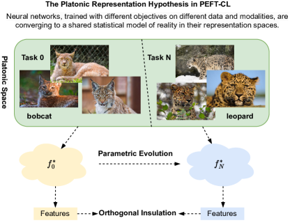
Figure 9: An explanation of the contradiction between highly similar classes across different tasks and the insulation of task-level feature orthogonality.

Researchers often question if ensuring orthogonality between features of different tasks might render the knowledge from previous tasks irrelevant, particularly when classes across tasks closely resemble each other. However, this perspective can be one-sided. Drawing on insights from [31], it is suggested that parameter spaces formed by different modalities and models tend to converge after extensive training—a concept we extend into the PEFT-CL context, illustrated in Fig. 9. This aligns with the principles of the Neural Tangent Kernel Regime, where $\Phi^{*}(X_{\tau},X_{k})=\Phi_{0}(X_{\tau},X_{k})=\Phi_{1}(X_{\tau},X_{k})=\cdots=\Phi_{\infty}(X_{\tau},X_{k})$. For similar classes, while they remain highly similar in Platonic Space, the mapping to a lower-dimensional space through varying sub-network component parameters over different periods ensures their distinction without compromising the transfer and preservation of knowledge within the Platonic Space.

References

- [1] Ibrahim Alabdulmohsin, Hartmut Maennel, and Daniel Keysers. The impact of reinitialization on generalization in convolutional neural networks. arXiv preprint arXiv:2109.00267, 2021.
- [2] Peter L Bartlett and Shahar Mendelson. Rademacher and gaussian complexities: Risk bounds and structural results. Journal of Machine Learning Research, 3(Nov):463–482, 2002.
- [3] Mehdi Abbana Bennani, Thang Doan, and Masashi Sugiyama. Generalisation guarantees for continual learning with orthogonal gradient descent. arXiv preprint arXiv:2006.11942, 2020.
- [4] Prashant Shivaram Bhat, Bharath Chennamkulam Renjith, Elahe Arani, and Bahram Zonooz. IMEX-reg: Implicit-explicit regularization in the function space for continual learning. Transactions on Machine Learning Research, 2024.
- [5] Blake Bordelon, Abdulkadir Canatar, and Cengiz Pehlevan. Spectrum dependent learning curves in kernel regression and wide neural networks. In International Conference on Machine Learning, pages 1024–1034. PMLR, 2020.
- [6] Tom Brown, Benjamin Mann, Nick Ryder, Melanie Subbiah, Jared D Kaplan, Prafulla Dhariwal, Arvind Neelakantan, Pranav Shyam, Girish Sastry, Amanda Askell, et al. Language models are few-shot learners. Advances in Neural Information Processing Systems, 33:1877–1901, 2020.
- [7] Pietro Buzzega, Matteo Boschini, Angelo Porrello, Davide Abati, and Simone Calderara. Dark experience for general continual learning: a strong, simple baseline. Advances in Neural Information Processing Systems, 33:15920–15930, 2020.
- [8] Abdulkadir Canatar, Blake Bordelon, and Cengiz Pehlevan. Spectral bias and task-model alignment explain generalization in kernel regression and infinitely wide neural networks. Nature Communications, 12(1):2914, 2021.
- [9] Mathilde Caron, Hugo Touvron, Ishan Misra, Hervé Jégou, Julien Mairal, Piotr Bojanowski, and Armand Joulin. Emerging properties in self-supervised vision transformers. In Proceedings of the IEEE/CVF International Conference on Computer Vision, pages 9650–9660, 2021.
- [10] Kian Chai. Generalization errors and learning curves for regression with multi-task gaussian processes. Advances in Neural Information Processing Systems, 22:279–287, 2009.
- [11] Chun-Fu Richard Chen, Quanfu Fan, and Rameswar Panda. Crossvit: Cross-attention multi-scale vision transformer for image classification. In Proceedings of the IEEE/CVF International Conference on Computer Vision, pages 357–366, 2021.
- [12] Lenaic Chizat, Edouard Oyallon, and Francis Bach. On lazy training in differentiable programming. Advances in Neural Information Processing Systems, 32:2937–2947, 2019.
- [13] Matthias De Lange, Rahaf Aljundi, Marc Masana, Sarah Parisot, Xu Jia, Aleš Leonardis, Gregory Slabaugh, and Tinne Tuytelaars. A continual learning survey: Defying forgetting in classification tasks. IEEE Transactions on Pattern Analysis and Machine Intelligence, 44(7):3366–3385, 2022.
- [14] Puneesh Deora, Rouzbeh Ghaderi, Hossein Taheri, and Christos Thrampoulidis. On the optimization and generalization of multi-head attention. arXiv preprint arXiv:2310.12680, 2023.
- [15] Ning Ding, Yujia Qin, Guang Yang, Fuchao Wei, Zonghan Yang, Yusheng Su, Shengding Hu, Yulin Chen, Chi-Min Chan, Weize Chen, et al. Parameter-efficient fine-tuning of large-scale pre-trained language models. Nature Machine Intelligence, 5(3):220–235, 2023.
- [16] Thang Doan, Mehdi Abbana Bennani, Bogdan Mazoure, Guillaume Rabusseau, and Pierre Alquier. A theoretical analysis of catastrophic forgetting through the ntk overlap matrix. In International Conference on Artificial Intelligence and Statistics, pages 1072–1080. PMLR, 2021.
- [17] Pierre Foret, Ariel Kleiner, Hossein Mobahi, and Behnam Neyshabur. Sharpness-aware minimization for efficiently improving generalization. arXiv preprint arXiv:2010.01412, 2020.
- [18] Rui Gao and Weiwei Liu. Ddgr: Continual learning with deep diffusion-based generative replay. In International Conference on Machine Learning, pages 10744–10763. PMLR, 2023.
- [19] Zhanxin Gao, Jun Cen, and Xiaobin Chang. Consistent prompting for rehearsal-free continual learning. In Proceedings of the IEEE/CVF Conference on Computer Vision and Pattern Recognition, pages 28463–28473, 2024.
- [20] Zeyu Han, Chao Gao, Jinyang Liu, Sai Qian Zhang, et al. Parameter-efficient fine-tuning for large models: A comprehensive survey. arXiv preprint arXiv:2403.14608, 2024.
- [21] Per Christian Hansen. The truncated svd as a method for regularization. BIT Numerical Mathematics, 27:534–553, 1987.
- [22] Jie Hao, Kaiyi Ji, and Mingrui Liu. Bilevel coreset selection in continual learning: A new formulation and algorithm. Advances in Neural Information Processing Systems, 36, 2024.
- [23] Kaiming He, Xinlei Chen, Saining Xie, Yanghao Li, Piotr Dollár, and Ross Girshick. Masked autoencoders are scalable vision learners. In Proceedings of the IEEE/CVF Conference on Computer Vision and Pattern Recognition, pages 16000–16009, 2022.
- [24] Patrick Helber, Benjamin Bischke, Andreas Dengel, and Damian Borth. Introducing eurosat: A novel dataset and deep learning benchmark for land use and land cover classification. In IEEE International Geoscience and Remote Sensing Symposium, pages 204–207. IEEE, 2018.
- [25] Dan Hendrycks, Kevin Zhao, Steven Basart, Jacob Steinhardt, and Dawn Song. Natural adversarial examples. In Proceedings of the IEEE/CVF Conference on Computer Vision and Pattern Recognition, pages 15262–15271, 2021.
- [26] Neil Houlsby, Andrei Giurgiu, Stanislaw Jastrzebski, Bruna Morrone, Quentin De Laroussilhe, Andrea Gesmundo, Mona Attariyan, and Sylvain Gelly. Parameter-efficient transfer learning for nlp. In International Conference on Machine Learning, pages 2790–2799. PMLR, 2019.
- [27] Edward J Hu, Yelong Shen, Phillip Wallis, Zeyuan Allen-Zhu, Yuanzhi Li, Shean Wang, Lu Wang, and Weizhu Chen. LoRA: Low-rank adaptation of large language models. In International Conference on Learning Representations, 2022.
- [28] Tianyang Hu, Wenjia Wang, Cong Lin, and Guang Cheng. Regularization matters: A nonparametric perspective on overparametrized neural network. In International Conference on Artificial Intelligence and Statistics, pages 829–837. PMLR, 2021.
- [29] Wei-Cheng Huang, Chun-Fu Chen, and Hsiang Hsu. OVOR: Oneprompt with virtual outlier regularization for rehearsal-free class-incremental learning. In International Conference on Learning Representations, 2024.
- [30] David Hughes, Marcel Salathé, et al. An open access repository of images on plant health to enable the development of mobile disease diagnostics. arXiv preprint arXiv:1511.08060, 2015.
- [31] Minyoung Huh, Brian Cheung, Tongzhou Wang, and Phillip Isola. The platonic representation hypothesis. arXiv preprint arXiv:2405.07987, 2024.
- [32] Arthur Jacot, Franck Gabriel, and Clément Hongler. Neural tangent kernel: Convergence and generalization in neural networks. In Advances in Neural Information Processing Systems, pages 8571–8580, 2018.
- [33] Zhong Ji, Jin Li, Qiang Wang, and Zhongfei Zhang. Complementary calibration: Boosting general continual learning with collaborative distillation and self-supervision. IEEE Transactions on Image Processing, 32:657–667, 2022.
- [34] Chao Jia, Yinfei Yang, Ye Xia, Yi-Ting Chen, Zarana Parekh, Hieu Pham, Quoc Le, Yun-Hsuan Sung, Zhen Li, and Tom Duerig. Scaling up visual and vision-language representation learning with noisy text supervision. In International Conference on Machine Learning, pages 4904–4916. PMLR, 2021.
- [35] Menglin Jia, Luming Tang, Bor-Chun Chen, Claire Cardie, Serge Belongie, Bharath Hariharan, and Ser-Nam Lim. Visual prompt tuning. In European Conference on Computer Vision, pages 709–727. Springer, 2022.
- [36] Dahuin Jung, Dongyoon Han, Jihwan Bang, and Hwanjun Song. Generating instance-level prompts for rehearsal-free continual learning. In Proceedings of the IEEE/CVF International Conference on Computer Vision, pages 11847–11857, 2023.
- [37] Ryo Karakida and Shotaro Akaho. Learning curves for continual learning in neural networks: Self-knowledge transfer and forgetting. In International Conference on Learning Representations, 2021.
- [38] Alex Krizhevsky, Geoffrey Hinton, et al. Learning multiple layers of features from tiny images. 2009.
- [39] Muhammad Rifki Kurniawan, Xiang Song, Zhiheng Ma, Yuhang He, Yihong Gong, Yang Qi, and Xing Wei. Evolving parameterized prompt memory for continual learning. In Proceedings of the AAAI Conference on Artificial Intelligence, volume 38, pages 13301–13309, 2024.
- [40] Jaehoon Lee, Yasaman Bahri, Roman Novak, Samuel S Schoenholz, Jeffrey Pennington, and Jascha Sohl-Dickstein. Deep neural networks as gaussian processes. arXiv preprint arXiv:1711.00165, 2017.
- [41] Jaehoon Lee, Samuel Schoenholz, Jeffrey Pennington, Ben Adlam, Lechao Xiao, Roman Novak, and Jascha Sohl-Dickstein. Finite versus infinite neural networks: an empirical study. Advances in Neural Information Processing Systems, 33:15156–15172, 2020.
- [42] Jaehoon Lee, Lechao Xiao, Samuel S Schoenholz, Yasaman Bahri, Jascha Sohl-Dickstein, and Jeffrey Pennington. Wide neural networks of any depth evolve as linear models under gradient descent. In Advances in Neural Information Processing Systems, pages 8572–8583, 2019.
- [43] Depeng Li and Zhigang Zeng. Crnet: A fast continual learning framework with random theory. IEEE Transactions on Pattern Analysis and Machine Intelligence, 45(9):10731–10744, 2023.
- [44] Jiyong Li, Dilshod Azizov, LI Yang, and Shangsong Liang. Contrastive continual learning with importance sampling and prototype-instance relation distillation. In Proceedings of the AAAI Conference on Artificial Intelligence, volume 38, pages 13554–13562, 2024.
- [45] Jin Li, Zhong Ji, Gang Wang, Qiang Wang, and Feng Gao. Learning from students: Online contrastive distillation network for general continual learning. In IJCAI, pages 3215–3221, 2022.
- [46] Xiaorong Li, Shipeng Wang, Jian Sun, and Zongben Xu. Variational data-free knowledge distillation for continual learning. IEEE Transactions on Pattern Analysis and Machine Intelligence, 45(10):12618–12634, 2023.
- [47] Xiang Lisa Li and Percy Liang. Prefix-tuning: Optimizing continuous prompts for generation. arXiv preprint arXiv:2101.00190, 2021.
- [48] Yan-Shuo Liang and Wu-Jun Li. Inflora: Interference-free low-rank adaptation for continual learning. arXiv preprint arXiv:2404.00228, 2024.
- [49] Sen Lin, Peizhong Ju, Yingbin Liang, and Ness Shroff. Theory on forgetting and generalization of continual learning. In International Conference on Machine Learning, pages 21078–21100. PMLR, 2023.
- [50] Yong Lin, Lu Tan, Hangyu Lin, Zeming Zheng, Renjie Pi, Jipeng Zhang, Shizhe Diao, Haoxiang Wang, Han Zhao, Yuan Yao, et al. Speciality vs generality: An empirical study on catastrophic forgetting in fine-tuning foundation models. arXiv preprint arXiv:2309.06256, 2023.
- [51] Xuanyuan Luo, Bei Luo, and Jian Li. Generalization bounds for gradient methods via discrete and continuous prior. Advances in Neural Information Processing Systems, 35:10600–10614, 2022.
- [52] Simone Magistri, Tomaso Trinci, Albin Soutif, Joost van de Weijer, and Andrew D. Bagdanov. Elastic feature consolidation for cold start exemplar-free incremental learning. In International Conference on Learning Representations, 2024.
- [53] Marc Masana, Xialei Liu, Bartłomiej Twardowski, Mikel Menta, Andrew D. Bagdanov, and Joost van de Weijer. Class-incremental learning: Survey and performance evaluation on image classification. IEEE Transactions on Pattern Analysis and Machine Intelligence, 45(5):5513–5533, 2023.
- [54] Michael McCloskey and Neal J Cohen. Catastrophic interference in connectionist networks: The sequential learning problem. In Psychology of learning and motivation, volume 24, pages 109–165. Elsevier, 1989.
- [55] James Mercer. Xvi. functions of positive and negative type, and their connection the theory of integral equations. Philosophical Transactions of the Royal Society of London. Series A, containing papers of a mathematical or physical character, 209(441-458):415–446, 1909.
- [56] Michael Murray, Hui Jin, Benjamin Bowman, and Guido Montufar. Characterizing the spectrum of the NTK via a power series expansion. In International Conference on Learning Representations, 2023.
- [57] Aaron van den Oord, Yazhe Li, and Oriol Vinyals. Representation learning with contrastive predictive coding. arXiv preprint arXiv:1807.03748, 2018.
- [58] Omkar M Parkhi, Andrea Vedaldi, Andrew Zisserman, and CV Jawahar. Cats and dogs. In Proceedings of the IEEE/CVF Conference on Computer Vision and Pattern Recognition, pages 3498–3505. IEEE, 2012.
- [59] Xingchao Peng, Qinxun Bai, Xide Xia, Zijun Huang, Kate Saenko, and Bo Wang. Moment matching for multi-source domain adaptation. In Proceedings of the IEEE/CVF International Conference on Computer Vision, pages 1406–1415, 2019.
- [60] Quang Pham, Chenghao Liu, and Steven C. H. Hoi. Continual learning, fast and slow. IEEE Transactions on Pattern Analysis and Machine Intelligence, 46(1):134–149, 2024.
- [61] Konstantin Pogorelov, Kristin Ranheim Randel, Carsten Griwodz, Sigrun Losada Eskeland, Thomas de Lange, Dag Johansen, Concetto Spampinato, Duc-Tien Dang-Nguyen, Mathias Lux, Peter Thelin Schmidt, et al. Kvasir: A multi-class image dataset for computer aided gastrointestinal disease detection. In Proceedings of the 8th ACM on Multimedia Systems Conference, pages 164–169, 2017.
- [62] Jingyang Qiao, Xin Tan, Chengwei Chen, Yanyun Qu, Yong Peng, Yuan Xie, et al. Prompt gradient projection for continual learning. In International Conference on Learning Representations, 2023.
- [63] Alec Radford, Jong Wook Kim, Chris Hallacy, Aditya Ramesh, Gabriel Goh, Sandhini Agarwal, Girish Sastry, Amanda Askell, Pamela Mishkin, Jack Clark, et al. Learning transferable visual models from natural language supervision. In International Conference on Machine Learning, pages 8748–8763. PMLR, 2021.
- [64] Krishnan Raghavan and Prasanna Balaprakash. Formalizing the generalization-forgetting trade-off in continual learning. Advances in Neural Information Processing Systems, 34:17284–17297, 2021.
- [65] Vijaya Raghavan T Ramkumar, Bahram Zonooz, and Elahe Arani. The effectiveness of random forgetting for robust generalization. arXiv preprint arXiv:2402.11733, 2024.
- [66] Sylvestre-Alvise Rebuffi, Alexander Kolesnikov, Georg Sperl, and Christoph H Lampert. icarl: Incremental classifier and representation learning. In Proceedings of the IEEE conference on Computer Vision and Pattern Recognition, pages 2001–2010, 2017.
- [67] Tal Ridnik, Emanuel Ben-Baruch, Asaf Noy, and Lihi Zelnik-Manor. Imagenet-21k pretraining for the masses. arXiv preprint arXiv:2104.10972, 2021.
- [68] Tim GJ Rudner, Freddie Bickford Smith, Qixuan Feng, Yee Whye Teh, and Yarin Gal. Continual learning via sequential function-space variational inference. In International Conference on Machine Learning, pages 18871–18887. PMLR, 2022.
- [69] Grzegorz Rypeść, Sebastian Cygert, Valeriya Khan, Tomasz Trzcinski, Bartosz Michał Zieliński, and Bartłomiej Twardowski. Divide and not forget: Ensemble of selectively trained experts in continual learning. In International Conference on Learning Representations, 2024.
- [70] Jack Sherman and Winifred J Morrison. Adjustment of an inverse matrix corresponding to a change in one element of a given matrix. The Annals of Mathematical Statistics, 21(1):124–127, 1950.
- [71] James Seale Smith, Leonid Karlinsky, Vyshnavi Gutta, Paola Cascante-Bonilla, Donghyun Kim, Assaf Arbelle, Rameswar Panda, Rogerio Feris, and Zsolt Kira. Coda-prompt: Continual decomposed attention-based prompting for rehearsal-free continual learning. In Proceedings of the IEEE/CVF Conference on Computer Vision and Pattern Recognition, pages 11909–11919, 2023.
- [72] Peter Sollich. Learning curves for gaussian processes. Advances in Neural Information Processing Systems, 11:344–350, 1998.
- [73] Yu-Ming Tang, Yi-Xing Peng, and Wei-Shi Zheng. When prompt-based incremental learning does not meet strong pretraining. In Proceedings of the IEEE/CVF International Conference on Computer Vision, pages 1706–1716, 2023.
- [74] Dmitry Ulyanov, Andrea Vedaldi, and Victor Lempitsky. Deep image prior. In Proceedings of the IEEE/CVF Conference on Computer Vision and Pattern Recognition, pages 9446–9454, 2018.
- [75] Nikhil Vyas, Yamini Bansal, and Preetum Nakkiran. Limitations of the ntk for understanding generalization in deep learning. arXiv preprint arXiv:2206.10012, 2022.
- [76] Haixin Wang, Xinlong Yang, Jianlong Chang, Dian Jin, Jinan Sun, Shikun Zhang, Xiao Luo, and Qi Tian. Parameter-efficient tuning of large-scale multimodal foundation model. Advances in Neural Information Processing Systems, 36, 2024.
- [77] Liyuan Wang, Jingyi Xie, Xingxing Zhang, Mingyi Huang, Hang Su, and Jun Zhu. Hierarchical decomposition of prompt-based continual learning: Rethinking obscured sub-optimality. Advances in Neural Information Processing Systems, 36, 2024.
- [78] Liyuan Wang, Xingxing Zhang, Hang Su, and Jun Zhu. A comprehensive survey of continual learning: Theory, method and application. IEEE Transactions on Pattern Analysis and Machine Intelligence, 46(8):5362–5383, 2024.
- [79] Yabin Wang, Zhiwu Huang, and Xiaopeng Hong. S-prompts learning with pre-trained transformers: An occam’s razor for domain incremental learning. Advances in Neural Information Processing Systems, 35:5682–5695, 2022.
- [80] Zhenyi Wang, Li Shen, Tiehang Duan, Qiuling Suo, Le Fang, Wei Liu, and Mingchen Gao. Distributionally robust memory evolution with generalized divergence for continual learning. IEEE Transactions on Pattern Analysis and Machine Intelligence, 45(12):14337–14352, 2023.
- [81] Zifeng Wang, Zizhao Zhang, Sayna Ebrahimi, Ruoxi Sun, Han Zhang, Chen-Yu Lee, Xiaoqi Ren, Guolong Su, Vincent Perot, Jennifer Dy, et al. Dualprompt: Complementary prompting for rehearsal-free continual learning. In European Conference on Computer Vision, pages 631–648. Springer, 2022.
- [82] Zifeng Wang, Zizhao Zhang, Chen-Yu Lee, Han Zhang, Ruoxi Sun, Xiaoqi Ren, Guolong Su, Vincent Perot, Jennifer Dy, and Tomas Pfister. Learning to prompt for continual learning. In Proceedings of the IEEE/CVF Conference on Computer Vision and Pattern Recognition, pages 139–149, 2022.
- [83] Alexander Wei, Wei Hu, and Jacob Steinhardt. More than a toy: Random matrix models predict how real-world neural representations generalize, 2022.
- [84] Jinlin Xiang and Eli Shlizerman. Tkil: tangent kernel approach for class balanced incremental learning. arXiv preprint arXiv:2206.08492, 2022.
- [85] Yi Xin, Siqi Luo, Haodi Zhou, Junlong Du, Xiaohong Liu, Yue Fan, Qing Li, and Yuntao Du. Parameter-efficient fine-tuning for pre-trained vision models: A survey. arXiv preprint arXiv:2402.02242, 2024.
- [86] Jialu Xing, Jianping Liu, Jian Wang, Lulu Sun, Xi Chen, Xunxun Gu, and Yingfei Wang. A survey of efficient fine-tuning methods for vision-language models—prompt and adapter. Computers & Graphics, 119:103885, 2024.
- [87] Ju Xu, Jin Ma, Xuesong Gao, and Zhanxing Zhu. Adaptive progressive continual learning. IEEE Transactions on Pattern Analysis and Machine Intelligence, 44(10):6715–6728, 2022.
- [88] HongWei Yan, Liyuan Wang, Kaisheng Ma, and Yi Zhong. Orchestrate latent expertise: Advancing online continual learning with multi-level supervision and reverse self-distillation. arXiv preprint arXiv:2404.00417, 2024.
- [89] Boyu Yang, Mingbao Lin, Yunxiao Zhang, Binghao Liu, Xiaodan Liang, Rongrong Ji, and Qixiang Ye. Dynamic support network for few-shot class incremental learning. IEEE Transactions on Pattern Analysis and Machine Intelligence, 45(3):2945–2951, 2022.
- [90] Fei Yang, Kai Wang, and Joost van de Weijer. Scrollnet: Dynamicweight importance for continual learning. In Proceedings of the IEEE/CVF International Conference on Computer Vision, pages 3345–3355, 2023.
- [91] Greg Yang. Scaling limits of wide neural networks with weight sharing: Gaussian process behavior, gradient independence, and neural tangent kernel derivation. arXiv preprint arXiv:1902.04760, 2019.
- [92] Greg Yang. Tensor programs ii: Neural tangent kernel for any architecture. arXiv preprint arXiv:2006.14548, 2020.
- [93] Greg Yang and Etai Littwin. Tensor programs iib: Architectural universality of neural tangent kernel training dynamics. In International Conference on Machine Learning, pages 11762–11772. PMLR, 2021.
- [94] Haoran Yang, Yumeng Zhang, Jiaqi Xu, Hongyuan Lu, Pheng Ann Heng, and Wai Lam. Unveiling the generalization power of fine-tuned large language models. arXiv preprint arXiv:2403.09162, 2024.
- [95] Ya-Ting C Yang, Timothy J Newby, and Robert L Bill. Using socratic questioning to promote critical thinking skills through asynchronous discussion forums in distance learning environments. The American journal of distance education, 19(3):163–181, 2005.
- [96] Elad Ben Zaken, Shauli Ravfogel, and Yoav Goldberg. Bitfit: Simple parameter-efficient fine-tuning for transformer-based masked language-models. arXiv preprint arXiv:2106.10199, 2021.
- [97] Jiang-Tian Zhai, Xialei Liu, Lu Yu, and Ming-Ming Cheng. Fine-grained knowledge selection and restoration for non-exemplar class incremental learning. In Proceedings of the AAAI Conference on Artificial Intelligence, volume 38, pages 6971–6978, 2024.
- [98] Xiaohua Zhai, Joan Puigcerver, Alexander Kolesnikov, Pierre Ruyssen, Carlos Riquelme, Mario Lucic, Josip Djolonga, Andre Susano Pinto, Maxim Neumann, Alexey Dosovitskiy, et al. A large-scale study of representation learning with the visual task adaptation benchmark. arXiv preprint arXiv:1910.04867, 2019.
- [99] Peiyan Zhang, Yuchen Yan, Chaozhuo Li, Senzhang Wang, Xing Xie, Guojie Song, and Sunghun Kim. Continual learning on dynamic graphs via parameter isolation. In Proceedings of the 46th International ACM SIGIR Conference on Research and Development in Information Retrieval, pages 601–611, 2023.
- [100] Da-Wei Zhou, Hai-Long Sun, Han-Jia Ye, and De-Chuan Zhan. Expandable subspace ensemble for pre-trained model-based class-incremental learning. In Proceedings of the IEEE/CVF Conference on Computer Vision and Pattern Recognition, pages 23554–23564, 2024.
- [101] Jinghao Zhou, Chen Wei, Huiyu Wang, Wei Shen, Cihang Xie, Alan Yuille, and Tao Kong. ibot: Image bert pre-training with online tokenizer. arXiv preprint arXiv:2111.07832, 2021.
- [102] Kaiyang Zhou, Jingkang Yang, Chen Change Loy, and Ziwei Liu. Learning to prompt for vision-language models. International Journal of Computer Vision, 130(9):2337–2348, 2022.
- [103] Wenda Zhou, Victor Veitch, Morgane Austern, Ryan P Adams, and Peter Orbanz. Non-vacuous generalization bounds at the imagenet scale: a pac-bayesian compression approach. arXiv preprint arXiv:1804.05862, 2018.