Discovery of a Damped Ly$\alpha$ Absorber in the Circumnuclear Zone of the FeLoBAL Quasar SDSS J083942.11+380526.3

Abstract

SDSS J083942.11+380526.3 ($z=2.315$) is a FeLoBAL quasar that exhibits visible Balmer absorption lines (H$\alpha$), implying a significant $n=2$ population. The quasar also shows an array of absorption lines, including O I, Ni II, Fe II, Mg II, Al III  to C IV and N V. The high-ionization absorption lines such as C IV and Si IV are revealed by slightly blueshifted BAL troughs. The resonance doublets such as Mg II and Al III are saturated but did not reached zero intensity which indicates that the BLR is partially covered. Overall, however, the absorption is predominantly from low-ionization Fe II lines, emitted from ground and excited states up to at least 3.814 eV. This implies that the absorbing gas spans the hydrogen ionization front and extends into the partially ionized zone where neutral hydrogen is certainly present. Notably, the hydrogen line spectrum of the quasar shows no signature of expected Ly$\alpha$ absorption. Instead, the line spectrum shows an unusual Ly$\alpha$ emission characterized by a fully filled emission line spectrum which is a composite of a strong narrow core superposed on a weak broad base. Taking into account the effect of partial covering to BLR, we have extracted a strong DLA trough in Ly$\alpha$ emission region. To fit the spectrum, we performed photoionized model calculations and compared them to the observations. We found that photoionization modeling using CLOUDY can successfully reproduce the main characteristics of the quasar spectrum, and the predicted neutral hydrogen column density arising from the clouds responsible for the low-ionization absorption provides a good match to the extracted DLA trough. This indicates that both the DLA and the low-ionization absorption arise from the same medium that is roughly collocated with the dusty torus.

1 Introduction

Quasar absorption line systems are excellent probes of both the physical properties of the absorbing gas intrinsic to the quasars (intrinsic absorbers, which are physically related to the quasars) and the distribution of gaseous clouds in the universe (intervening absorbers or host galaxy gas, which are unrelated to the quasar). These systems are primarily described by their neutral hydrogen column density.

Quasar spectra often show a plethora of absorption lines that are detached from or adjacent to the emission lines. These absorption lines are imprinted on the quasar spectra. Based on linewidths, the traditional broad absorption lines (BALs) are absorptions exhibited in the spectra of Quasars with velocity widths more than $2000\hbox{~{}km~{}s${}^{-1}$}$, and blueshifted by up to $\sim 0.2c$ relative to systemic redshift (Weymann, Carswell, & Smith, 1981). BALs are generally understood to form in high-velocity outflows, possibly connected with accretion disk winds (Murray et al., 1995; de Kool & Begelman, 1995; Tombesi et al., 2010). However, Arav et al. (2018) found that at least $50\%$ of BALQSO outflows are at distances greater than 100 pc from the central source, and at least $12\%$ are at distances greater than 1 kpc. Based on the ions producing the absorptions, BALs are further classified as High-ionization BALs (HiBALs), low-ionization BALs (LoBALs), or iron low-ionization BALs (FeLoBALs) (Trump et al., 2006). The majority of BALs show absorption only from highly ionized species such as C IV , N V , and O VI  (typically identified through the presence of C IV absorption) and are referred to as HiBALs. A minority of BALs, known as LoBALs, also exhibit absorption from lower ionized species such as Mg II, and Al III. A small subset of LoBALs, called FeLoBALs, additionally show absorption from excited fine-structure levels or excited levels of Fe II and/or Fe III (Hazard et al., 1987; Hall et al., 2002). Additionally, the rarest absorption features in BALs are found in a handful of objects that exhibit absorption in their Balmer lines (Hutchings et al., 2002; Aoki et al., 2006; Hall, 2007; Zhang et al., 2015; Shi et al., 2016a; Schulze et al., 2018).

Recently, in the first paper of a series of four, Choi et al. (2022) presented a detailed analysis of the outflows in 50 low-redshift ($0.66<z<1.63$) FeLoBAL quasars using SimBAL, a novel spectral-synthesis modeling software (Leighly et al., 2018). The authors identified a group of eleven FeLoBAL quasars, a new class dubbed loitering outflow objects. These are characterized by low outflow velocities and high column density winds located close to the central engine, within the vicinity of the torus. The authors also found that FeLoBAL quasars with Balmer absorption are only found in BALs with log $R\lesssim 1$ [pc], suggesting that the presence of Balmer absorption lines can be used as an indicator for compact broad absorption line (BAL) winds (small log $R$ with high densities).

The term “damped Lyman absorption" simply describes a phenomenon where the column density of neutral hydrogen is sufficient to show damping wings. Damped Ly$\alpha$ systems (DLAs) are historically defined as having a neutral hydrogen column density $N_{\mathrm{H\,\textsc{i}}}$$\geq 2\times 10^{20}\,\mathrm{cm}^{-2}$ (Wolfe et al., 1986). Depending on their origin with respect to the background sources, DLAs observed in the spectra of quasars can be divided into an entity either entirely separate from the quasar (intervening DLA) or loosely associated with the quasar (proximate DLA). Intervening DLAs are produced by neutral hydrogen gas located by chance along the line of sight to the background sources without being related to the sources themselves (Noterdaeme et al., 2019). They were initially observed in QSO spectra and typically originate in the H I regions of the high-redshift progenitors of present-day spiral galaxies (Wolfe et al., 1986) or dwarf galaxies (Tyson, 1988).

Associated DLAs may arise either in galaxies neighboring the quasar host or from H I clouds within the quasar host galaxy itself. Finley et al. (2013) found a population of proximate DLAs (PDLAs) that do not fully cover the Ly$\alpha$ emission region of the background quasar (see also Jiang et al., 2016; Xie et al., 2018). In some extreme cases, a new class of PDLAs called ghostly DLAs as reported by Fathivavsari et al. (2017), has been described in the literature (see also Fathivavsari, 2020; Laloux & Petitjean, 2021). In the case of ghostly DLAs, the BLR is not fully covered and the absorption system is only detected through its Ly$\beta$, Ly$\gamma$ and higher series lines as well as metal absorption lines (metal-selected). These ghostly DLAs are expected to be located closest to the central engine.

Additionally, associated DLAs are also common in long-duration gamma-ray burst (GRB) afterglow spectra, typically with much higher column densities at the burst redshift than it is observed in QSO-DLAs (Vreeswijk et al., 2004; Watson et al., 2006). The extremely large H I column densities observed in many GRB-DLAs suggest an origin related to the host galaxy, presumably the GRBs’ star-forming region.

DLAs are also characterized by the presence of multiple absorption lines from low ionization species such as Fe II, Si II, Ni II, and Zn II, which are in their dominant ionization stages. The presence of the rare line transitions (e.g., He I*, Balmer series, excited fine-structure and other metastable, excited-state lines such as C II*, C III*, Si II*, Ni II*, Fe II*) whether related to BAL systems or associated with DLA absorbers, can be used as various indicators or diagnostics, for example (1) Zn II  can be used as a metallicity indicator (Zsargó & Federman 1998 and references therein), (2) He I* absorption lines are very useful diagnostics for the geometry and physical conditions of the absorbing gas in quasars (Leighly, Dietrich, & Barber, 2011; Liu et al., 2015), (3) the C III* $\lambda$1175 multiplet lines or Si II and Si II* lines pairs can be valuable density diagnostic (Gabel et al., 2005b; Hamann et al., 2019). Combining the density with photoionization modeling can be used to estimate the location of the absorbing gas, acting as a distance indicator, (4) FeLoBAL quasars with Balmer absorption can be used as an indicator for compact BAL winds (Choi et al., 2022), (5) in cases of partial covering, the observed depths of saturated lines are direct indicators of the covering fractions of optically-thick gas in that transition (Shi et al., 2016b; Hamann et al., 2019).

As is well known, absorption spectrum is an one-dimensional probe of the absorbers along our line of sight towards a quasar. Conversely, emission line profiles encompass spatially integrated contributions, offering crucial spatial and kinematic insights into the structure of the line emitters. To explore the spatial and kinematic structure of the DLAs, our initial step involves detecting the Ly$\alpha$ emission line. A few rare examples of detecting the residual flux in the DLA trough have been reported in the literature. However, the diverse origins of the flux within the DLA trough pose a challenge for their physical interpretation (Barnes & Haehnelt, 2009; Hennawi et al., 2009; Noterdaeme et al., 2014).

In this paper, we report another “loitering" outflow FeLoBAL quasar SDSS J083942.11+380526.3 (hereafter SDSS J0839+3805). The UV spectrum of SDSS J0839+3805 includes an array of absorption lines, predominantly low-ionization Fe II lines, emitted from ground and excited states up to at least 3.814 eV which appeared to be overlapping troughs. The quasar also exhibits saturated doublets absorption with partial coverage of the BLR. The $K$- and $JH$-band spectra of SDSS J0839+3805 obtained with CISCO on the Subaru telescope also show Balmer and He I* $\lambda$3889 absorption (Aoki et al., 2006). The presence of a wide variety of absorption lines from a broad range of ions, especially rare features like Balmer series, He I*, excited fine-structure and excited-state lines, can place firm constraints on the physical properties and location of the outflowing gas. We conducted a comprehensive analysis of the spectrum of SDSS J0839+3805 and performed photoionized model calculations and compared them to the observations.

The paper is organized as follows. In Section 2, we describe the observational data and analysis methods. An overview of the spectrum is presented in Section 3. We developed a template fitting procedure that is described in Section 4. A uniform density model and its caveats are presented in Section 5. In Section 6, we describe a turbulent, near-solar metallicity, two-component model and the results, while a more detailed information about atomic data of Fe II for four datasets which is used in photoionization calculations is presented in Appendix A. Discussion and summary are given in Section 7. Throughout the paper, we assume a cosmology consisting of $H_{0}=70\hbox{~{}km~{}s${}^{-1}$}\mathrm{Mpc}^{-1}$, $\Omega_{\mathrm{M}}=0.3$ and $\Omega_{\mathrm{\Lambda}}=0.7$.

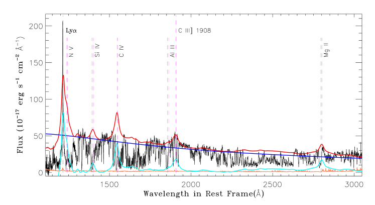
Figure 1: BOSS Spectrum of SDSS J0839+3805. We fitted EDR composite spectrum to the observed spectrum (in black) using an SMC extinction curve with flux at wavelength around 1324, 1350, 1480, 1960, 2238, 2645 Å and longward 3020 Å, that are regarded as continuum windows. The solid red/blue line represents the best fitted reddened EDR composite/continuum. The corresponding reddened emission lines are drawn in solid cyan line. The error spectrum (in coral) is also shown at the bottom.

2 Observations and Data Reduction

The object was observed four times by the Sloan Digital Sky Survey (SDSS) from February 2002 to February 2016, and none of these spectroscopic observations show any significant change during this 14 years period (4.2 years in the quasar rest-frame). We selected the best spectrum from the Baryon Oscillation Spectroscopic Survey (BOSS) of SDSS-III from DR10 as our primary for scientific analysis which was observed on Modified Julian Date 55508 (calendar date:11/8/2010) with plate No.3765 and fiber No.392. The spectrum covers a wavelength range of 3650 $\sim$ 10400 Å, and the resolution varies from $\sim$ 1500 at 3800 Å to $\sim$ 2500 at 9000 Å.

We applied a Galactic extinction correction to the spectrum using the mean extinction curve from Fitzpatrick & Massa (2007) with the Galactic reddening value, $E(B-V)=0.037$ which was evaluated based on the extinction map traced by Schlegel et al. (1998). We then converted the observed wavelengths and shifted the observed spectrum to the quasar rest-frame by replacing the cosmological redshift by the systemic redshift (z = 2.315, given in SDSS DR7 catalog). The rest-frame spectrum covers the wavelength range of 1085 $\sim$ 3130 Å.

3 Continuum Fitting and Features Overview

3.1 Continuum Fitting with a Composite Spectrum

We initiated the analysis by assessing the intrinsic reddening of the object in the quasar’s rest frame, employing an SMC extinction curve (Gordon et al., 2003). As a first approximation, we used the EDR composite spectrum (Vanden Berk et al., 2001) as a representation of the unabsorbed quasar spectrum (i.e., the spectrum of the central source before interaction with the gas clouds), and fitted it to the observed spectrum. For simplicity, we omitted intergalactic extinction and assume that all dust reddening beyond the Milky Way are intrinsic to the quasar. Considering the ubiquitous strong UV absorption lines in the observed spectrum, we fitted a power law (reddened) to a set of emission- and absorption-free regions of the quasar spectrum and then we tried to match the dereddened observed spectrum with the EDR composite spectrum using the nonlinear least-squares procedure, MPFIT (Markwardt, 2009), where we avoided the portions with strong line features to the greatest degree possible. If we consider the continuum points centered around 1324, 1350, 1480, 1960, 2238, 2645  Å , and longward of 3020  Å in the rest frame as continuum windows free of emission and absorption, the continuum points in both the composite spectrum and the dereddened SDSS J0839+3805 spectrum align with a power law. Following correction for intrinsic SMC-like reddening ($E(B-V)=0.03$), the best-fit power-law spectral index is determined to be $\alpha_{\lambda}=-1.46$. The best-fitting EDR composite and the power-law continuum (reddened) are plotted in Fig.1.

Table 1: Measured line Parameters Based On Double Gaussians Fitting.

Line	absorption-line center	FWHM	Ionic Column Density
	(km s-1)	(km s-1)	cm-2
Ni II $\lambda 1455$	$-245.2\pm 5.8$/$-598.3\pm 24.2$	$225.3\pm 13.2$/$251.5\pm 60.4$	$(2.24\pm 0.12)$e+15/$(4.98\pm 1.00)$e+14
Ni II* $\lambda 2207$	$-219.0\pm 5.8$/$-572.1\pm 20.7$	$249.1\pm 14.2$/$174.9^{\textbf{a}}$	$(2.67\pm 0.13)$e+14/$(3.72\pm 0.68)$e+13
Fe II* $\lambda 1761$	$-239.3\pm 8.0$/$-530.9\pm 18.4$	$197.9\pm 19.1$/$174.9^{\textbf{a}}$	$(4.20\pm 0.35)$e+14/$(1.45\pm 0.25)$e+14
Cr II $\lambda 2056$	$-253.3\pm 7.4$/$-567.9\pm 16.8$	$222.4\pm 17.2$/$229.1\pm 41.4$	$(3.44\pm 0.23)$e+14/$(1.40\pm 0.22)$e+14
Zn II $\lambda 2026$	$-230.6\pm 5.0$/$-624.\pm 17.9$	$230.1\pm 11.6$/$247.3\pm 56.0$	$(9.80\pm 0.44)$e+13/$(2.56\pm 0.44)$e+13
H I $\lambda 1215$	$-951.5\pm 9.9$/$-1493.8\pm 20.2$	$405.8\pm 17.7$/$512.5\pm 42.8$	$(3.10\pm 0.16)$e+14/$(2.08\pm 0.17)$e+14
H I $\lambda 1215^{\textbf{b}}$	$-953.3\pm 6.1$/$-1486.6\pm 13.8$	$365.6\pm 10.6$/$487.5\pm 27.4$	$(7.17\pm 0.26)$e+14/$(3.59\pm 0.19)$e+14
H$\alpha$	……	……	(2$\sim$3.2)e+13${}^{\textbf{c}}$
Notes. Ni II* $\lambda 2207$ and Fe II* $\lambda 1761$ transitions from lower levels at 1.254, 2.029 eV; ${}^{\textbf{a}}$ Upper limit set by the spectral resolution (R$\sim$1800).
${}^{\textbf{b}}$ The case for saturated Ly$\alpha$ absorptionon due to partial coverage to BLR; ${}^{\textbf{c}}$ cited from Aoki et al. (2006) –derived from the curve of growth.

3.2 An Overview of the Spectrum

The spectrum of SDSS J0839+3805 shows unusual Ly$\alpha$ emission features. The Ly$\alpha$ emission is represented by a composite of strong and intermediate velocity width cores superposed on a relatively weak broad base. As expected, the observed spectrum also shows numerous absorption lines from a broad range of ions, in particular, of C, N, O, Mg, Al, Si, P, Cr, Fe, Ni, and Zn, including Fe II*, and Ni II* from their excited states up to 3.814 eV and 1.859 eV, respectively. The high-ionization absorption lines, such as C IV $\lambda\lambda 1548,1551$, and Si IV $\lambda\lambda 1394,1403$ in the spectrum of quasar are appeared as BAL troughs near the center of the corresponding lines. These troughs span a similar velocity width of $\sim 2000\hbox{~{}km~{}s${}^{-1}$}$ from about 500 to $-1500\hbox{~{}km~{}s${}^{-1}$}$ with respect to the systemic velocity, and slightly shifted to the blueward of the corresponding emission lines. We also note that the two discrete absorption troughs in the blue wing of Ly$\alpha$ spectrum within BAL troughs of high-ionization lines are most likely due to Ly$\alpha$ absorptions. But we cannot exclude the possibility that the absorptions originate from unidentified lines. Also, there are several relatively narrower absorption lines from low-ionization species, such as Fe II, Si II, P II, S II, Ni II, Cr II, up to Zn II. Most of these lines are heavily blended together in the lower-resolution SDSS spectrum, partly due to the associated transitions being very close in wavelength, and partly due to unknown turbulent and/or velocity gradients broadening in the absorption gas.

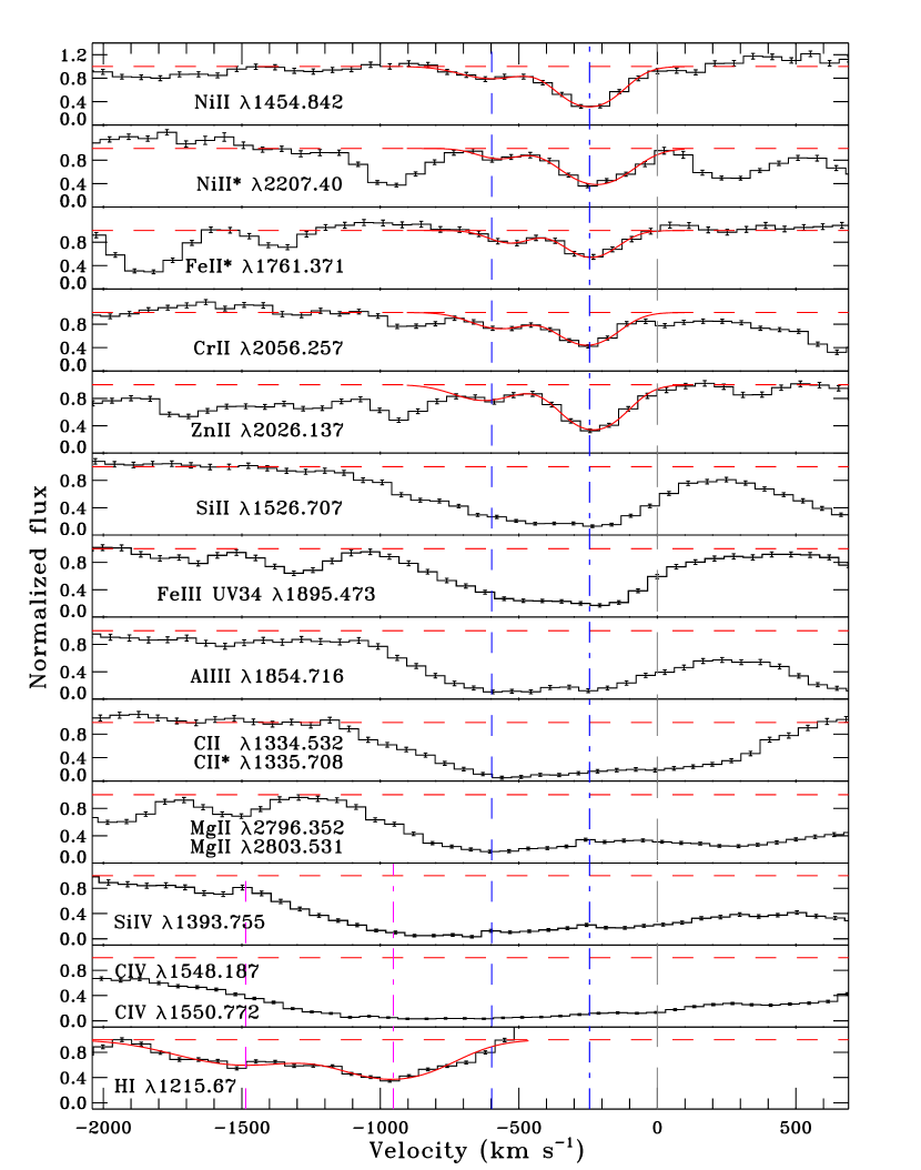
Figure 2: Normalized flux for some typical absorption lines and Gaussian fits to six resolved absorption profiles in velocity space. The composite spectrum is simply normalized to unity shown by dashed red horizontal lines. The black lines with $\pm 1\sigma$ error bars show the observed data. The solid red lines are fitted with a double Gaussian for six resolved low/high-ionization absorptions. The dot-dashed/dashed blue (magenta) vertical line marks the centroid velocities of fitted Gaussian profiles for Ni II $\lambda 1455$ (Ly$\alpha$) relative to the systemic redshift.

Fig. 2 shows the absorption profiles produced by ions, Ni II, Fe II, Cr II, Zn II, Si II, Fe III, Al III, C II, Mg II, Si IV, C IV, and H I. Gaussian fits to five resolved absorption profiles of Ni II $\lambda 1455$, Ni II* $\lambda 2207$, Fe II* $\lambda 1761$, Cr II $\lambda 2056$, and Zn II $\lambda 2026$ that have reasonable depth for low-ionization lines, as well as the resolved absorption profiles of Ly$\alpha$, are shown in solid red lines in both the first five and the last panels of the figure. The low-ionization lines show similar absorption profiles with two discrete velocity systems which are best fitted with a double Gaussian profile. For example, the fitted Gaussian profiles to Ni II $\lambda 1455$ give velocity shifts centered at $-245\pm 5.8\hbox{~{}km~{}s${}^{-1}$}$ and $-598\pm 24\hbox{~{}km~{}s${}^{-1}$}$ having full width at half-maximums (FWHM) of $225\pm 13\hbox{~{}km~{}s${}^{-1}$}$ and $252\pm 60\hbox{~{}km~{}s${}^{-1}$}$, respectively. The Ly$\alpha$ absorptions within BAL troughs of high-ionization lines can also be well fitted with a double Gaussian profile with a much higher blueshifted velocity. All these measurements are summarized in Table 1. These two components of low-ionization lines are also present in strong absorption lines of both singly ionized species such as: C II, Mg II, and Si II and doubly ionized species such as: Al III, and Fe III UV 34. The ratio of absorption depths varies significantly between the two components. The high-ionization absorptions (e.g., C IV, and Si IV ) exhibit BAL troughs that are much broader which fully encompass the velocity range of the low-ionization absorptions.

From an immediate inspection of the quasar spectrum, it is obvious that the resonance absorption lines (e.g., Mg II, Al III) are saturated but did not reach zero intensity (see Fig. 2), which indicates that the absorber has much higher column density and does not cover the background emission source completely. This high column density makes the usual much weaker lines from excited levels of Fe II and Ni II, and other less abundant iron group elements becoming detectable. This could greatly increase the number of narrow UV absorption lines from the low-ionization ions as expected for the observed spectrum of the quasar.

It is important to note the numerous absorption lines of Fe II which worth a brief description. The observed Fe II spectrum reveals approximately 80 Fe II multiplets, with identifications extending up to at least UV 283 within the wavelength range redward of the Ly$\alpha$ emission line (see Fig. 7). The main Fe II absorption features include:

1. The profiles of Fe II show that the depths of some strong absorption multiplets UV 1, UV 2, UV 3, and UV 62-63 near 2600 Å, 2382 Å, 2344 Å, and 2750 Å are somewhat shallower than that of the weak lines of UV 8 near 1635 Å, and several other weak multiplets (e.g. UV 9, UV 38, UV 41, UV 44-45).

2. Most of the transitions from 1550 to 1730  Å are due to Fe II UV 38-46, UV 8, UV 68 and UV 84 multiplets, etc. Redward of this region, some other relatively resolved multiplets (not all) are UV 4-5, UV 60, UV 64-5, UV 78, UV 83, UV 145, UV 148, UV 161, UV 180, UV 191, UV 217, UV 234-235, UV 261, UV 263, UV 283, etc.

Considering the huge number of Fe II lines, there must be some misidentifications.

4 Template Fitting Method

Considering the heavy blending of the absorption features of SDSS J0839+3805, we strategized to generate a synthetic spectrum to fit the observed absorption line spectrum. For the template, we made the assumption that the shape of the function that describes the optical depth as a function of velocity (for any transition) is the same for all lines (Korista et al., 1992; Arav et al., 2001). In order to construct the synthetic model, we considered both the level population and the kinematic structure.

4.1 Multicomponent Fitting

Based on the ionization structure, a constant density slab of gas irradiated by an ionizing continuum of an AGN is divided into two distinct zones: (1) a highly ionized H II zone (H II-zone) at the illuminated face of the slab, where hydrogen is almost completely ionized (the hydrogen Strömgren layer), and (2) an excited H I zone (H I*-zone) behind it, where a few to a few tens percent hydrogen is ionized (Collin-Souffrin et al., 1986). Thus, almost all of the elements such as Fe, Ni and Zn are in singly ionized form in the partially ionized zone, whereas the doubly ionized species such as Al III, are present in the Strömgren layer but still get accumulated in considerable amounts inside the partially ionized zone (de Kool et al., 2002).

The residual intensities measured at the lowest points (to avoid contamination from unknown emission to the utmost) in the saturated troughs of various transitions range from near zero (e.g., C II $\lambda 1334$, C IV) to $\sim 0.2/0.4$ (e.g., Mg II) relative to full/broad emission. Also, a significant residual is present in the saturated low-ionization absorptions in strong broad emission line ranges (e.g., Si II $\lambda 1526$ in the blue wing of the C IV broad emission lines). Therefore, a more complicated multicomponent model for the background emission and stratified absorber must be taken into account.

The background AGN emission is generally thought to be composed of a featureless continuum and a plethora of broad and narrow emission lines. However, the physically distinct sources (i.e., a continuum source and emission-line regions) have different sizes and geometries, thus, the covering factors can not be the same for all. Thus, in some cases, where the total background emission is only partially covered by the absorber, different viewing angle toward the distinct sources with different sizes would give different covering factors (Barlow & Sargent, 1997; Gabel et al., 2005a). Here, we model the background emission from the BLR and the compact accretion disk, separately. The BLR is further divided into two emitting regions of lower and higher ionization lines, which is consistent with a radially stratified ionization structure of BLR. This is supported by reverberation mapping studies which confirms that the emitting region of low ionization lines formed several times farther out than that of higher ionization lines (Clavel et al., 1991). Thus, we applied separate covering factors, ${}^{\rm b}C_{\rm j}^{i}$ and ${}^{\rm d}C_{\rm j}^{i}$ for the BLR and the disk, where the superscript i stands for the number of radially stratified layers in the absorbing gas along the line of sight, and the subscript j defines the different emitting regions of the source (e.g., the lower/higher ionization region of the BLR).

As for example, if we consider three layers of the absorber where the covering factor decreases monotonically in the radial direction, then the observed residual flux can be given by the following equation:

$$F_{j=l,h}= \sum_{k=b,d}F_{k}\Big{[}\ ^{\rm k}C_{\rm j}^{3}\prod_{i=1}^{3}e^{-\tau_{i}}+1-^{\rm k}C_{\rm j}^{1}+^{\rm k}C_{\rm j}^{1}(^{\rm k}C_{\rm j}^{1}-^{\rm k}C_{\rm j}^{2})e^{-\tau_{1}}$$ (1)

$$+\ ^{\rm k}C_{\rm j}^{2}(^{\rm k}C_{\rm j}^{2}-\ ^{\rm k}C_{\rm j}^{3})\prod_{i=1}^{2}e^{-\tau_{i}}\Big{]},$$

where, $F_{b}$ and $F_{d}$ are the intrinsic broad emission-line and continuum fluxes, respectively.

Dividing equation (1) by $F_{b}+F_{d}$ gives

$$I_{j=l,h}= \sum_{k=b,d}R_{k}\Big{[}\ ^{\rm k}C_{\rm j}^{3}\prod_{i=1}^{3}e^{-\tau_{i}}+1-^{\rm k}C_{\rm j}^{1}+^{\rm k}C_{\rm j}^{1}(^{\rm k}C_{\rm j}^{1}-^{\rm k}C_{\rm j}^{2})e^{-\tau_{1}}$$ (2)

$$+\ ^{\rm k}C_{\rm j}^{2}(^{\rm k}C_{\rm j}^{2}-\ ^{\rm k}C_{\rm j}^{3})\prod_{i=1}^{2}e^{-\tau_{i}}\Big{]},$$

where, $R_{b,d}=F_{b,d}/(F_{b}+F_{d})$ is the normalized flux of the broad emission-line/continuum to the total intrinsic flux. These two equations can be easily extended to cases where the absorber is composed of more than three layers.

Using these equations with Cloudy, we developed a new algorithm that enables us to calculate the absorptions due to a continuous stratified medium, as well as a simplified compilation of atomic data that includes energy levels, wavelengths, and oscillator strengths of the transitions of selected ions from the National Institute of Standards and Technology Atomic Spectra Database (NIST)¹. In our compilation, we also added some observational results of line transitions that are available in the literature (Morton, 1991, 2003; Fedchak & Lawler, 1999; Cashman et al., 2017).

For SDSS J0839+3805, it is reasonable to assume that the absorber fully covers the continuum source and partially covers the BLR. We also assume that both the H II-zone and H I*-zone have two sub-components, each having the same covering factor, ${}^{\rm b}C_{\rm j}^{0}=\ ^{\rm b}C_{\rm j}^{1}$ and ${}^{\rm b}C_{\rm j}^{2}=\ ^{\rm b}C_{\rm j}^{3}$. For an absorber composed of four layers with zero as initial value of i, the equations (1) and (2) can be simplified as

$$F_{j=l,h}\ = F_{d}\prod_{i=0}^{3}e^{-\tau_{i}}+F_{b}\Big{[}\ ^{\rm b}C_{\rm j}^{3}\prod_{i=0}^{3}e^{-\tau_{i}}+1-\ ^{\rm b}C_{\rm j}^{0}$$ (3)

$$+\ ^{\rm b}C_{\rm j}^{1}(^{\rm b}C_{\rm j}^{1}-\ ^{\rm b}C_{\rm j}^{2})\prod_{i=0}^{1}e^{-\tau_{i}}\Big{]},$$

$$I_{j=l,h}\ = R_{d}\prod_{i=0}^{3}e^{-\tau_{i}}+R_{b}\Big{[}\ ^{\rm b}C_{\rm j}^{3}\prod_{i=0}^{3}e^{-\tau_{i}}+1-\ ^{\rm b}C_{\rm j}^{0}$$ (4)

$$+\ ^{\rm b}C_{\rm j}^{1}(^{\rm b}C_{\rm j}^{1}-\ ^{\rm b}C_{\rm j}^{2})\prod_{i=0}^{1}e^{-\tau_{i}}\Big{]},$$

The factor is defined as fraction of the background light source(s) subtended by the absorbing cloud as seen by the observer. The observed depths of saturated lines are direct indicator of the covering fractions of optically thick clouds in that transition. Similarly, we can measure the uncovering fractions from the ratios of the measured residual intensities at the lowest points in the absorption troughs to the emission source. The covering factors used for the calculation are estimated by using the representative absorption lines of C II $\lambda 1334$, Si II $\lambda 1526$, C IV $\lambda 1548$, and Mg II $\lambda 2796$ which are expected to be completely saturated. The measured covering factors are ${}^{\rm d}C=1$, ${}^{\rm b}C_{h}^{0,1}=0.96$, ${}^{\rm b}C_{l}^{0,1}=0.83$, and ${}^{\rm b}C_{h}^{2,3}=0.74$, ${}^{\rm b}C_{l}^{2,3}=0.64$.

4.2 Optical Depth Template and Photoionization Simulations.

To construct the synthetic model, not only the kinematic structure but also the level populations were required. An essential ingredient required by the synthetic model is the optical depth template that describes the optical depth as a function of velocity extracted from the reference absorption line profile. This template is best derived from the observed profile of an unblended absorption line of intermediate depth that occurs in a part of the spectrum where the continuum is well defined, especially in the relatively smooth part of the spectrum free of broad emission lines. Once the optical depth template is known, the optical depth as a function of velocity for any transition is the same as that for the optical depth template with any arbitrary scale factor. The scale factors or “multipliers” for other ions are identical to the ratios of the ionic column densities of associated ions to that of the reference ion. The level populations of all ions that give rise to absorption lines in the spectrum can be calculated using the large-scale synthesis code Cloudy (version 17.02, Ferland et al. (2017)).

We choose Ni II $\lambda 1455$ absorption from the ground level as our optical depth template for low-ionization absorption lines. This absorption has two discrete velocity systems that were fitted with a double Gaussian profile. We found obvious redshifted absorptions (see also Choi et al., 2022) in the wavelength ranges, N V $\lambda 1242$ to S II $\lambda 1250$ and C IV $\lambda 1550$ to Fe II $\lambda 1559$ in the red wings of high-ionization absorption lines, N V and C IV (see Fig. 7). Presumably these absorptions might be produced by highly ionized gas in an inflow (Wu et al. 2024, in preparation). Due to heavy saturation and low resolution, we did not fit the high-ionization absorption troughs with a theoretical model. Instead, we choose a Gaussian for an outflow besides a template absorption from Ly$\alpha$ at relatively high blueshifted velocity of $\sim 1000\hbox{~{}km~{}s${}^{-1}$}$. These were manually adjusted to get a suitable absorptions desired in the troughs of C IV and N V.

The absorbing cloud was modeled as plane-parallel slab of gas exposed to ionizing radiation from the central engine, where the gas is assumed to have an uniform density and chemical composition. Initially, we applied solar abundance and zero turbulence, and the medium was assumed to be free of dust. The photoionization model was parameterized by ionization parameter $U$, number density of hydrogen, $n_{\mathrm{H}}$ and column density of hydrogen, $N_{\mathrm{H}}$. A continuum similar to that deduced by Mathews & Ferland (1987) was used as incident ionizing radiation (see also Hamann et al. (2013); Sarkar et al. (2021) for the influence from different SEDs). To reproduce the complex Fe II absorption, we incorporated the full 371 levels $\mathrm{Fe}^{+}$ model in our simulation, including all levels up to 11.59 eV². To evaluate the accuracy of atomic data of Fe II, we have introduced a comparison of atomic data for selected lines of Fe II for four datasets from Verner et al. (1999), Smyth et al. (2019), Tayal & Zatsarinny (2018) and CHIANTI³. Some of these results from the latter three datasets were incorporated into the atomic data of Fe II (see Appendix A for further details) to produce synthetic Fe II spectra.

Initially, we generated a grid of photoionization models in the $U$-$n_{\mathrm{H}}$-$N_{\mathrm{H}}$ space with the parameter ranges, $-4<\log\,U<4$, $0<\log\,n_{\mathrm{H}}(\mathrm{cm}^{-3})<15$, and $19<\log\,N_{\mathrm{H}}(\mathrm{cm}^{-2})<24$ in steps of 0.2 dex for all of them. Among all the models in the initial grid of parameters, the gridpoints, which generate a synthetic spectrum with smallest $\chi^{2}$ compared to the observed spectrum were found. This allowed us to obtain a rough estimate of the parameter ranges. Then, a fine grid with halved increment was calculated by relaxing the assumptions of zero turbulence and solar abundance using the code Cloudy (version 17.02, Ferland et al. (2017)). This step helped us to narrow down the allowed values in the parameter space neighboring the found gridpoints to further constrain the absorber’s properties.

5 A Uniform Density Model and Its Caveats

The observed spectrum of SDSS J0839+3805 shows numerous absorption lines which provides an unique opportunity to place firm constraint on the absorber’s physical properties by simultaneously taking account of as many absorption lines as possible. The photoionization simulations for a small range of parameters can closely reproduce most of the observed spectrum features in the synthetic spectra.

5.1 A Uniform, Homogeneous Absorber

We performed a series of photoionization calculations using the code Cloudy and compared the output to the observations. In photoionization modeling, first we adopted a uniform density model, mainly focused on low-ionization absorption lines. The synthetic spectrum includes contributions from H I, He I, C II, C III, C IV, N V, O I, Mg II, Al II, Al III, Si II, Si III, Si IV, P II, P III, S II, S III, Ti III, Cr II, Mn II, Fe II, Fe III, Co II, Ni II and Zn II. Ionic column densities for some typical lines and emission-line ratios of C IV/Ly$\alpha$ and N V/Ly$\alpha$ predicted by photoionization simulations are listed in Table 2. The metallicity and turbulent velocity are considered as free parameters. Among the models with $\log\,n_{\mathrm{H}}(\mathrm{cm}^{-3})=7.0$, the solar metallicity models can be ruled out by our data. The subsolar metallicity models yield acceptable results as a whole, except that the ionic column density of H$\alpha$/Zn II is much higher/lower than the observed data. Model #7 with $\log\,U=-1.2$, $\log\,n_{\mathrm{H}}(\mathrm{cm}^{-3})=6.6$, and $\log\,N_{\mathrm{H}}(\mathrm{cm}^{-2})=22.3$ for which we adopted solar metallicity of $Z=Z_{\odot}$ and turbulent velocity, $v=50\hbox{~{}km~{}s${}^{-1}$}$ seems roughly in agreement with the observation. However, this model overpredicts the ionic column densities of ground and low excitation levels of Fe II, and Ni II, and thus, we referred it as “preliminary” solution for the uniform density model. The photoionization modeling yields a radial distance of $R_{\mathrm{abs}}\approx$ 32 pc from the nucleus for the absorbing clouds (see Section 6.2).

Table 2: A Uniform, Homogeneous Absorber Model.

Model

Turbulence

Metallicity

Predicted Ionic Column Density

Emission-line Ratio

$\log(U/n_{\rm H}/N_{\rm H})$

(km s-1)

(Z⊙)

Ly$\alpha$

H$\alpha$

Zn II

Fe II

Fe II UV191

Al III

Si IV

C IV/Ly$\alpha$

N V/Ly$\alpha$

#1: -1.3/7.0/22.30

0

1

9.66e+21

8.69e+13

1.55e+14

6.09e+16

6.09e+13

3.60e+15

9.48e+16

0.26

0.008

#2: -1.3/7.0/22.30

100

1

9.91e+21

4.52e+13

1.51e+14

5.88e+16

1.82e+14

3.74e+15

9.42e+16

0.26

0.014

#3: -1.3/7.0/22.00

100

1

2.17e+21

1.29e+13

2.48e+13

1.51e+16

8.70e+13

1.90e+15

9.68e+16

0.27

0.014

#4: -1.15/7.0/22.35

50

0.3

8.23e+21

1.46e+14

1.75e+13

1.68e+16

9.71e+13

1.54e+15

3.81e+16

0.30

0.013

#5: -1.15/7.0/22.35

100

0.3

8.42e+21

1.02e+14

1.67e+13

1.68e+16

1.23e+14

1.59e+15

3.79e+16

0.30

0.016

#6: -1.20/6.6/22.30

0

1

8.33e+21

3.36e+13

1.19e+14

6.08e+16

2.79e+13

3.57e+15

1.17e+17

0.25

0.009

#7: -1.20/6.6/22.30

50

1

8.48e+21

2.26e+13

1.17e+14

6.10e+16

7.28e+13

3.65e+15

1.16e+17

0.243

0.013

#8: -1.20/6.6/22.30

100

1

8.56e+21

1.74e+13

1.15e+14

6.09e+16

9.74e+13

3.71e+15

1.16e+17

0.248

0.016

Notes. All the predicted ionic column densities correspond to the ground level except for Fe II UV191;

The predicted emission-line ratios include contributions from resonance-line doublets C IV $\lambda\lambda 1548,1550$ and N V $\lambda\lambda 1238,1242$.

5.2 DLA Trough and Ly$\alpha$-like Emissions

In the Ly$\alpha$ emission line range, the apparent lack of Ly$\alpha$ absorption trough is an artifact of comparing them to the prominent broad H$\alpha$ emission detected in the NIR Subaru CISCO data with blueshifted absorption (Aoki et al., 2006).

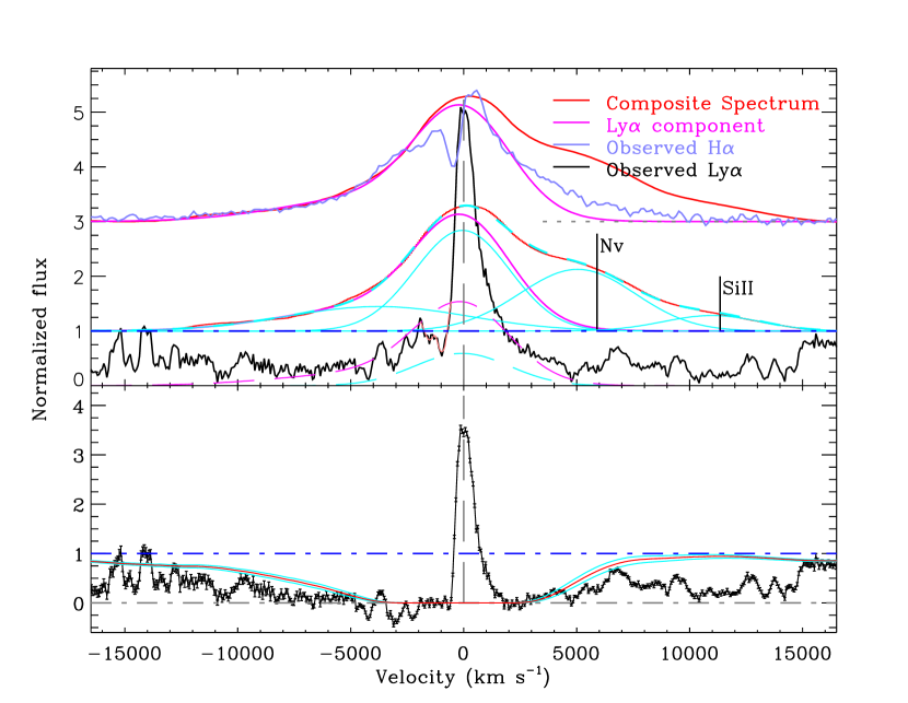
Figure 3: Decomposition of the Ly$\alpha$ spectral region and the DLA trough in velocity space. Top panel shows the similarity between the observed broad emission line profile and the model predicted profile of Ly$\alpha$ in magenta long dashes line which represents the residual flux due to partial covering of the BLR. Bottom panel shows a strong DLA trough with an emission core obtained by subtracting the residual flux from the observed spectrum (black line). The theoretical Voigt profiles for $\log\,N_{\mathrm{H\,\textsc{i}}}(\mathrm{cm}^{-2})=21.95\pm 0.05$ predicted by photoionization modeling are shown in red and cyan.

Fig. 3 shows the detection of an unusual DLA system where an exceptionally intense Ly$\alpha$ emission superposed on the trough of the DLA in quasar SDSS J0839+3805. All of the spectra are normalized to unity in the continuum levels (dot-dashed blue horizontal line). Here, a single power-law approximation (solid blue line in Fig.1) clearly fails on the blue wing of Ly$\alpha$ emission. Thus, a broken power-law is needed to fit the continuum. We fitted a linear continuum constrained by the EDR flux at two points $\lambda$ = 1157.5 and 1283.6  Å, that are relatively uncontaminated with line emission features. The EDR flux is consistent with the maximum measured flux near these two points within uncertainty of 0.05 dex. For simplicity, we neglected the influence of accumulated averaged Ly$\alpha$ forest absorption on the intrinsic spectrum of the quasar. The subtraction of broad Ly$\alpha$ emission and the blends with N V and possibly Si II are dealt with by means of multiple Gaussian profile decompositions. The decompositions of four Gaussian components (solid cyan line), the broad Ly$\alpha$ (solid magenta line) feature which can be modeled by a combination of two Gaussians of the four components, and observed (black line) spectra in the Ly$\alpha$ spectral region are presented in the upper panel of Fig. 3. The magenta/cyan long dashes line represents the uncovering fractions of the corresponding component. The Ly$\alpha$ absorptions which are best fitted with a double Gaussian profile in a weak broad base are drawn in coral solid line. The broad H$\alpha$ emission drawn in light blue solid line that are offset by +2 is overplotted in the figure for comparison. The composite spectrum assumption is justified by the consistency between Ly$\alpha$ subtraction and the observed H$\alpha$ emission. The profile of the observed Ly$\alpha$ emission, except for the narrow core, is consistent with the magenta long dashes line being scaled by uncovering factors that manifests itself as the residual flux due to partial coverage of the BLR.

The residual of the broad wings of the Ly$\alpha$ emission is much below the continuum intensity, suggesting strong Ly$\alpha$ absorption. We extracted a strong DLA trough (the lower panel of Fig. 3) with a prominent Ly$\alpha$ emission located near the center of the trough by subtracting the residual flux due to partial covering effects, from the observed spectrum. The over absorptions in the DLA trough, blueward of Ly$\alpha$ emission may be deduced from extra absorptions such as: BLR clouds, etc. This is beyond the scope of this paper. Other uncertainties can be introduced by the difference between the intrinsic absorption-free and the composite spectrum, due to data calibration noises, etc. Considering both the numerous low ionization absorption lines and strong Ly$\alpha$ emission in the observed spectrum, the Voigt profile is consistent, at least qualitatively, with the observed data.

In the extracted DLA trough, there is a strong intermediate width Ly$\alpha$ emission with a rest equivalent width (EW) and FWHM of $14.4\pm 1.1$ Å, and $897\pm 69\hbox{~{}km~{}s${}^{-1}$}$, respectively. The Ly$\alpha$ line shows an asymmetric profile having a sharp blueward cutoff and an extended red wing over a range of $\sim$ 2000 km s^-1 from about $-$500 to 1500 km s^-1 with respect to systemic velocity. This velocity range contrary to BAL troughs (from about 500 to $-1500\hbox{~{}km~{}s${}^{-1}$}$) shows an opposite trend with the similar velocity width. If the absorption troughs of certain resonance lines in the spectrum of SDSS J0839+3805 are produced by pure scattering then they must be compensated by an equal amount of emission. We shall tentatively assume that the outflow is axisymmetric (see Scargle, Caroff, & Noerdlinger 1970 for a spherically symmetric expanding envelope). Then, the photons scattered from the half of the approching windflow (the near side) will be blueshifted, while scattering from the receding half (the far side) will be redshifted and distributed over a similar frequency interval. A summation of absorption and scattering form the total line profile that consists of absorption with an emission wing to the red. This profile resemble P Cygni profile (i.e., an undisplaced emission line with a blueshifted absorption component). The Ly$\alpha$ emission and blueshifted absorption lines extend to about the same velocity range ($\sim$ 2000 km s^-1), and together they resemble P Cygni profiles, suggesting self-absorption (Crenshaw & Kraemer, 2007).

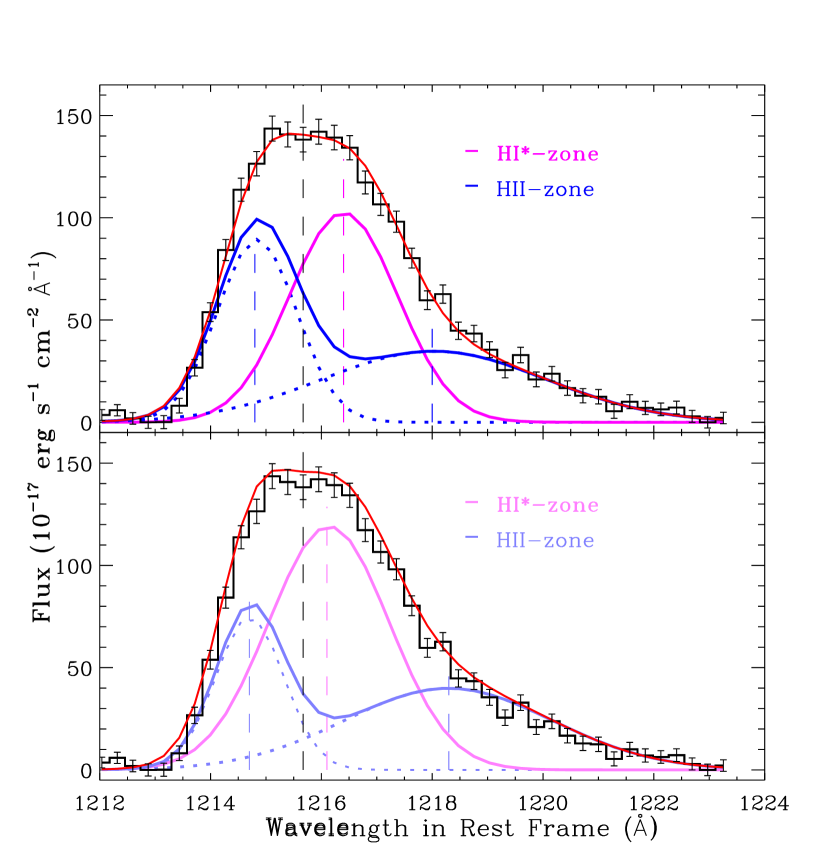
Figure 4: Three Gaussian profile decompositions of Ly$\alpha$ emission core obtained by subtracting the residual flux from the observed spectrum. Top panel: the intermediate width Ly$\alpha$ emission has been fitted with three Gaussians centered at the rest wavelengths of 1214.8, 1216.4 and 1218.0 Å with peak values $\sim$ 89.4, 101.9 and 34.7, respectively. We further assumed that these three Gaussians are divided into two categories based on the emitting region. Bottom panel: another decomposition of Ly$\alpha$ emission with three gaussians centered at the rest wavelengths of 1214.7, 1216.1 and 1218.3 Å with peak values $\sim$ 74.7, 118.2 and 39.4, respectively.

Fig. 4 shows three Gaussian fittings of the Ly$\alpha$ emission. Top panel shows the intermediate width Ly$\alpha$ emission was fitted with three Gaussians of FWHMs $\sim$ 416.8, 564.9, and 1170.9  km s^-1centered at the rest wavelengths of 1214.8, 1216.4 and 1218.0 Å with peak values of $\sim$ 89.4, 101.9 and 34.7, respectively. Furthermore, we assumed a priori that these three Gaussians are divided into two categories based on the emitting region; the middle Gaussian profile was produced in H I*-zone and a double-peaked profile consisting of the other two Gaussians was produced in H II-zone (see the next section for an analysis of legitimizing the assumption). Note that this fitting is quite subjective and is based upon visual inspection. Bottom panel of Fig. 4 is another decomposition of Ly$\alpha$ emission with three gaussians centered at the rest wavelengths of 1214.7, 1216.1 and 1218.3 Å with peak values $\sim$ 74.7, 118.2 and 39.4, respectively.

This emitter ought to be seen from other intercepting ions (e.g. C IV, N V) by resonance line scattering and fluorescent emission due to reprocessing of the nuclear continuum radiation. Detailed analysis of the residual intensities in the C IV and N V troughs led to the conclusions that there indeed exist significant double-peaked Ly$\alpha$-like emission in C IV and N V troughs. In addition to the double-peaked component, the residual intensity in C IV trough had revealed a prominent Gaussian component similar to that seen in Ly$\alpha$ emission (i.e., H I*-zone component) despite having a relatively reduced line efficiency. These results are in contradiction with the profile of Ly$\alpha$ emission from uniform density model as a whole.

Although the synthetic spectrum from the photoionization models roughly fit the observed spectrum, there are some discrepancies in the model predictions for an absorber with a much smaller radial thickness ($\Delta{R}/R\sim 10^{-4}$, here the radial thickness is measured using $\Delta{R}\sim N_{\rm H}/n_{\rm H}$) and extremely low ratio of the N V to Ly$\alpha$ emergent line intensities (see Table 2).

6 A Two-component Model and The Results

A uniform density model overestimates the ionic column densities of ground and low excitation levels of Fe II, and Ni II, as well as underestimate N V emission. The predicted emission-line ratios of N V/Ly$\alpha$ by photoionization simulations from a uniform density model should be less than two percent at most (see Table 2). We, thus relaxed the assumption of uniform density to get a more physically plausible condition of the absorbing gas. The specific steps are: we first fixed the location and density of H I*-zone to those calculated in preliminary solution for a uniform density model, and then allowed the density of H II-zone to decrease as the ionization parameter increases. Eventually, this increases the radial thickness of the absorber leading to a negligible influence on the H I*-zone behind it. A two-density model of the H II-zone with $\log\,U=1.0$, $\log\,n_{\mathrm{H}}(\mathrm{cm}^{-3})=4.5$, and $\log\,N_{\mathrm{H}}(\mathrm{cm}^{-2})=23.5$, followed by H I*-zone behind it with $\log\,n_{\mathrm{H}}(\mathrm{cm}^{-3})=6.6$, and $\log\,N_{\mathrm{H}}(\mathrm{cm}^{-2})=22.25$ with a solar metallicity and turbulence, $v=100\hbox{~{}km~{}s${}^{-1}$}$ could partly solve the problem that occurred in a uniform density model, without significantly influencing the following region.

6.1 A Turbulent, Near-solar Metallicity, Two-component Model

To clarify the nature of the two-component model, we generated a grid of refined models in the $U$-$n_{\mathrm{H}}$-$N_{\mathrm{H}}$ space with the ranges, $0<\log\,U<1.5$, $4<\log\,n_{\mathrm{H}}(\mathrm{cm}^{-3})<9$, and $22.6<\log\,N_{\mathrm{H}}(\mathrm{cm}^{-2})<24$ in steps of 0.1 dex for all the three parameters with turbulence, $v=100\hbox{~{}km~{}s${}^{-1}$}$ using Cloudy.

A two-component model constructed with photoionization modeling by using the combined absorption and emission-line ratios that arise from the same gas is shown in Fig. 5.

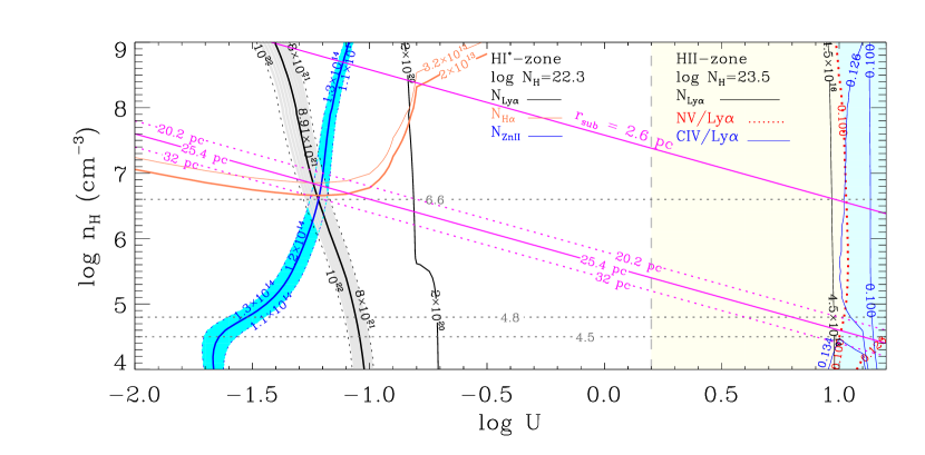
Figure 5: A two-component model constructed with photoionization simulations by using the combined absorption line and emission-line ratios. The left part of the figure shows a strong DLA absorber constrained by the measured column densities of Zn II, and H$\alpha$ in H I*-zone. The right part shows the H II-zone located at a distance very similar to that of the DLA absorber which can at least partly produce the desired N V emission.

In the figure, the left part shows a strong DLA absorber in H I*-zone constrained by the measured column densities of Zn II, and H$\alpha$ (also see Tian et al., 2021, for the method used to determine parameters) and the right part shows a lesser dense gas in H II-zone located at a distance very similar to that of the DLA absorber which reveals a greatly enhanced emergent emission-line efficiency of N V. An obvious emergent line intensity of N V is detected in the observed spectrum. The dependency of the emission-line ratios of C IV/Ly$\alpha$ and N V/Ly$\alpha$ on their ionization parameters and densities predicted by photoionization simulations are shown in Fig. 6. Absorption lines of C IV, and N V are overplotted on the data. We found that manual adjustments and iteration by trial and error provide more flexibility in situations where the line profiles are irregular and the blending is potentially severe. This way a reasonable fit to the C IV profile can be obtained for a range of $\sim 15.9-17$ for $\log\,N_{\rm C\,\textsc{iv}}(\mathrm{cm}^{-2})$.

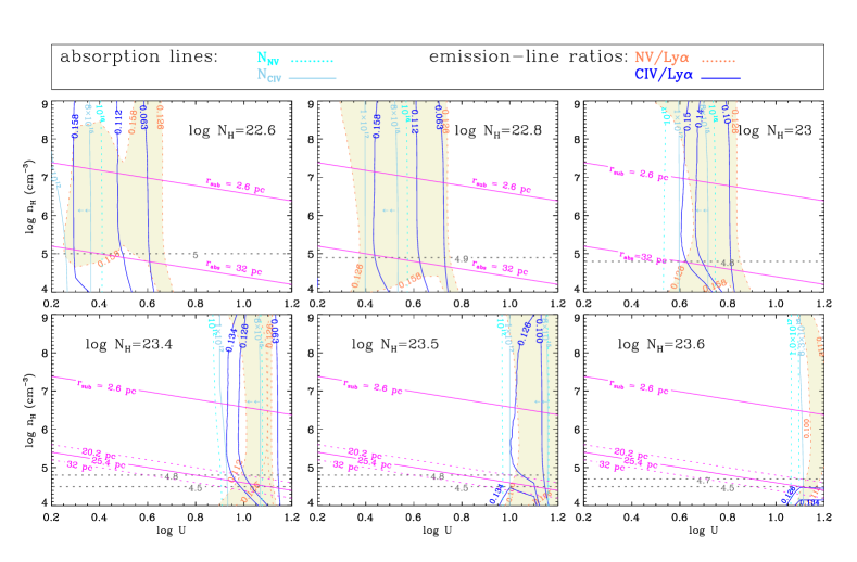
Figure 6: The model parameters constrained both by the emission-line ratios and absorption lines. The dependence of the predicted emission-line ratios of C IV/Ly$\alpha$ and N V/Ly$\alpha$ on their ionization parameters and densities are shown. Overplotted on the data are absorption lines of C IV, and N V. A reasonable range of $\log\,N_{\rm C\,\textsc{iv}}(\mathrm{cm}^{-2})$ from $\sim 15.9$ to $17$ were obtained by manual adjustment and iteration by trial and error in order to fit the C IV profile.

Based on the similar distance reported above, we developed a continuous two-component model for the absorbing cloud. A model consisting of a continuous stratified medium which is divided into two zones; a highly ionized H II-zone where the clouds are exposed to the full ionizing continuum and a weakly ionized zone called the excited H I*-zone behind the H II-zone which is exposed only to the continuum filtered through the H II-zone. Using this model, we performed a series of photoionization equilibrium calculations for a range of model parameters ($\log(U/n_{\rm H}/N_{\rm H})$, turbulent velocity, and metallicity). Here, the turbulent velocity and metallicity were considered as free parameters by considering both the column densities of Fe II, and Ni II from highly excited levels which are sensitive to turbulent velocity, and from ground and relatively low excitation levels which are overestimated by solar metallicity models. The latter gives a clue that the metallicity of the absorbing cloud is probably below that of the solar. Table 3 lists the predicted column densities of some typical ions and emission-line ratios of the strong resonance-line doublets C IV $\lambda\lambda 1548,1550$ and N V $\lambda\lambda 1238,1242$ relative to Ly$\alpha$. It should be borne in mind, however, that the photoionization analysis and observational constraints on emission lines suffer from large uncertainties.

Table 3: A Two-component Model

Model	H II-zone								H I*-zone
	$\log(U/n_{\rm H}/N_{\rm H})$	Ly$\alpha$	C IV	N V	Si IV	N V/Ly$\alpha^{a}$	C IV/Ly$\alpha^{b}$		$\log(n_{\rm H}/N_{\mathrm{H\,\textsc{i}}})$	H$\alpha$	Zn II	Fe II UV191	Al III	N V/Ly$\alpha^{a}$	C IV/Ly$\alpha^{b}$
	Turbulent velocity $v$ = 100 km s-1, solar metallicity Z=Z⊙								Turbulent velocity $v$ = 100 km s-1, subsolar metallicity Z=0.5Z⊙
#1…	0.5/5.0/22.8	2.04e+16	1.07e+16	1.80e+16	2.98e+10	0.138/0.106	0.134/0.105		6.6/22.0	1.20e+13	1.09e+14	7.88e+13	1.61e+15	0.004/0.002	0.082/0.040
#2…	0.7/4.9/23.0	1.83e+16	9.35e+15	1.49e+16	4.82e+09	0.134/0.108	0.132/0.108		6.6/22.0	1.38e+13	1.34e+14	9.42e+13	1.38e+15	0.005/0.003	0.090/0.044
#3…	0.9/4.7/23.3	2.39e+16	2.52e+16	2.74e+16	3.74e+10	0.117/0.095	0.133/0.107		6.6/22.0	1.21e+13	1.75e+14	8.71e+13	9.82e+14	0.004/0.002	0.080/0.039
#4…	0.9/4.8/23.4	3.72e+16	1.33e+17	1.03e+17	3.26e+14	0.099/0.078	0.142/0.103		6.6/22.0	1.42e+13	1.88e+14	1.03e+14	8.72e+14	0.0004/0.0001	0.070/0.033
#5…	1.0/4.5/23.4	2.29e+16	2.18e+16	2.44e+16	1.03e+10	0.119/0.099	0.132/0.109		6.6/22.0	9.16e+12	1.83e+14	6.76e+13	8.79e+14	0.004/0.002	0.075/0.036
#6…	1.0/4.5/23.5	3.56e+16	8.94e+16	7.42e+16	1.08e+14	0.100/0.080	0.133/0.100		6.6/22.0	8.57e+12	1.92e+14	6.44e+13	7.81e+14	0.0006/0.0002	0.058/0.027
#7…	1.0/4.6/23.5	3.55e+16	8.93e+16	7.41e+16	1.05e+14	0.098/0.079	0.132/0.099		6.6/22.0	1.07e+13	1.93e+14	7.98e+13	8.06e+14	0.0008/0.0003	0.065/0.031
#8…	1.0/4.7/23.5	3.55e+16	8.91e+16	7.39e+16	1.03e+14	0.097/0.079	0.130/0.098		6.6/22.0	1.34e+13	1.94e+14	9.86e+13	8.31e+14	0.0012/0.0004	0.071/0.034
#9…	1.1/4.6/23.6	3.39e+16	6.99e+16	5.95e+16	2.60e+13	0.097/0.079	0.124/0.096		6.6/22.0	1.25e+13	1.99e+14	9.29e+13	8.01e+14	0.0018/0.0007	0.072/0.034
	Turbulent velocity $v$ = 50 km s-1, solar metallicity Z=Z⊙								Turbulent velocity $v$ = 50 km s-1, subsolar metallicity Z=0.5Z⊙
#10…	0.9/4.8/23.3	2.34e+16	2.47e+16	2.70e+16	3.12e+10	0.079/0.061	0.093/0.069		6.6/22.0	2.41e+13	1.83e+14	7.94e+13	9.66e+14	0.003/0.002	0.093/0.047
#11…	0.9/4.8/23.4	3.67e+16	1.20e+17	9.54e+16	2.53e+14	0.072/0.052	0.111/0.073		6.6/22.0	2.30e+13	1.95e+14	7.64e+13	8.34e+14	0.0006/0.0003	0.076/0.039
#12…	1.0/4.7/23.5	3.50e+16	8.45e+16	7.03e+16	7.25e+13	0.068/0.051	0.099/0.068		6.6/22.0	2.17e+13	2.02e+14	7.29e+13	7.92e+14	0.0011/0.0006	0.077/0.039
#13…	1.0/4.7/23.6	7.54e+16	1.72e+19	1.65e+17	1.07e+16	0.037/0.027	0.112/0.069		6.6/22.0	1.99e+13	2.07e+14	6.77e+13	6.90e+14	0.0000/0.0000	0.048/0.024
	Turbulent velocity $v$ = 100 km s-1, solar metallicity Z=Z⊙								Turbulent velocity $v$ = 100 km s-1, subsolar metallicity Z=0.3Z⊙
#14…	0.9/4.6/23.3	2.39e+16	2.52e+16	2.74e+16	3.75e+10	0.118/0.096	0.135/0.108		6.0/22.0	1.21e+13	9.29e+13	5.55e+13	7.79e+14	0.005/0.003	0.102/0.050
#14-1…	0.9/4.6/23.3	…							6.6/22.0	1.03e+13	1.05e+14	5.47e+13	6.25e+14	0.003/0.0015	0.084/0.041
#14-2…	0.9/4.6/23.3	…							7.0/22.0	1.02e+13	1.12e+14	5.42e+13	4.98e+14	0.0012/0.0004	0.055/0.026
#15…	1.0/4.5/23.5	3.56e+16	8.94e+16	7.42e+16	1.08e+14	0.0998/0.080	0.133/0.100		6.0/22.0	1.09e+13	1.11e+14	5.07e+13	6.28e+14	0.002/0.001	0.090/0.044
#15-1…	1.0/4.5/23.5	…							6.6/22.0	9.20e+12	1.17e+14	5.01e+13	5.05e+14	0.0004/0.0001	0.068/0.033
#15-2…	1.0/4.5/23.5	…							7.0/22.0	9.06e+12	1.21e+14	4.98e+13	4.19e+14	0.0001/0.0000	0.042/0.019
#16…	1.1/4.5/23.6	3.40e+16	6.99e+16	5.95e+16	2.65e+13	0.098/0.080	0.126/0.097		6.0/22.0	1.32e+13	1.12e+14	6.12e+13	6.59e+14	0.005/0.003	0.104/0.051
#16-1…	1.1/4.5/23.6	…							6.6/22.0	1.08e+13	1.21e+14	5.84e+13	5.01e+14	0.0010/0.0004	0.077/0.037
#16-2…	1.1/4.5/23.6	…							7.0/22.0	1.06e+13	1.23e+14	5.79e+13	4.28e+14	0.0003/0.0001	0.049/0.023
	Turbulent velocity $v$ = 100 km s-1, subsolar metallicity Z=0.8Z⊙								Turbulent velocity $v$ = 100 km s-1, subsolar metallicity Z=0.5Z⊙
#17…	0.7/5.0/23.2	3.23e+16	5.05e+16	4.32e+16	7.67e+11	0.108/0.082	0.149/0.105		6.6/21.9	1.28e+13	1.20e+14	9.92e+13	1.10e+15	0.0026/0.001	0.079/0.038
#18…	0.8/4.9/23.3	3.10e+16	4.25e+16	3.77e+16	2.59e+11	0.104/0.081	0.135/0.10		6.6/21.9	1.22e+13	1.30e+14	9.62e+13	1.01e+15	0.003/0.0014	0.079/0.038
#19…	0.9/4.8/23.4	3.00e+16	3.70e+16	3.38e+16	8.35e+10	0.101/0.080	0.126/0.096		6.6/22.0	1.45e+13	1.75e+14	1.04e+14	9.96e+14	0.0032/0.0015	0.080/0.039
#19-1…	0.9/4.8/23.4	…							6.6/21.9	1.16e+13	1.39e+14	9.26e+13	9.36e+14	0.0032/0.0016	0.080/0.039
#20…	1.0/4.8/23.5	2.92e+16	3.26e+16	3.06e+16	2.72e+10	0.098/0.079	0.117/0.093		6.6/22.0	1.71e+13	1.85e+14	1.22e+14	9.58e+14	0.004/0.002	0.087/0.042
#20-1…	1.0/4.8/23.5	…							6.6/21.9	1.37e+13	1.46e+14	1.08e+14	9.07e+14	0.004/0.002	0.087/0.042
#21…	1.1/4.7/23.6	2.85e+16	2.87e+16	2.78e+16	9.42e+09	0.096/0.080	0.112/0.091		6.6/22.0	1.59e+13	1.92e+14	1.15e+14	8.97e+14	0.004/0.002	0.089/0.043
	Turbulent velocity $v$ = 100 km s-1, subsolar metallicity Z=0.5Z⊙								Turbulent velocity $v$ = 100 km s-1, subsolar metallicity Z=0.5Z⊙
#22…	0.9/4.7/23.5	3.36e+16	2.61e+16	2.24e+16	2.73e+09	0.088/0.070	0.110/0.084		6.6/22.0	1.12e+13	1.61e+14	8.05e+13	1.06e+15	0.002/0.001	0.075/0.036
#23…	0.9/4.8/23.5	3.36e+16	2.61e+16	2.24e+16	2.73e+09	0.087/0.069	0.109/0.083		6.6/22.0	1.40e+13	1.60e+14	9.95e+13	1.11e+15	0.003/0.001	0.081/0.040
#24…	1.0/4.7/23.6	3.34e+16	2.27e+16	2.03e+16	9.98e+08	0.084/0.068	0.101/0.079		6.6/22.0	1.30e+13	1.70e+14	9.36e+13	1.01e+15	0.003/0.001	0.082/0.040
#25…	1.0/4.8/23.6	3.34e+16	2.27e+16	2.03e+16	9.99e+08	0.083/0.067	0.099/0.078		6.6/22.0	1.62e+13	1.70e+14	1.15e+14	1.05e+15	0.003/0.002	0.088/0.043
#26…	1.1/4.6/23.7	3.34e+16	2.07e+16	1.90e+16	4.27e+08	0.082/0.067	0.095/0.076		6.6/22.0	1.19e+13	1.79e+14	8.67e+13	9.22e+14	0.0028/0.0014	0.082/0.040
#27…	1.1/4.7/23.7	3.34e+16	2.07e+16	1.90e+16	4.26e+08	0.080/0.066	0.094/0.075		6.6/22.0	1.49e+13	1.80e+14	1.07e+14	9.58e+14	0.0032/0.0016	0.089/0.043
Notes. ${}^{\textbf{a}}$ the predicted emission-line ratios of N V $\lambda\lambda 1238,1242$ doublets relative to Ly$\alpha$; ${}^{\textbf{b}}$ the predicted emission-line ratios of C IV $\lambda\lambda 1548,1550$ doublets relative to Ly$\alpha$.

Among the models, model #19-1 consisting of a H II-zone with $\log\,U=0.9$, $\log\,n_{\mathrm{H}}(\mathrm{cm}^{-3})=4.8$, $\log\,N_{\mathrm{H}}(\mathrm{cm}^{-2})=23.4$, and Z = 0.8Z_⊙, followed by H I*-zone behind it with $\log\,n_{\mathrm{H}}(\mathrm{cm}^{-3})=6.6$, $\log\ N_{\mathrm{H\,\textsc{i}}}=21.9$, and Z = 0.5Z_⊙ with the same turbulent velocity of $v=100\hbox{~{}km~{}s${}^{-1}$}$ seemed in best agreement with the observed spectrum, and thus it was accepted as our final solution.

The optimized synthetic spectra constructed from Cloudy models using the fitting method used in our previous work (Shi et al., 2016b) are plotted in Fig. 7. The red line represents the synthetic absorption spectrum constructed from Cloudy model. The dotted and solid blue lines show the reddened EDR composite spectrum and power-law continuum, respectively. The synthetic emission spectra of strong resonance line doublets C IV $\lambda\lambda 1548,1550$, and N V $\lambda\lambda 1238,1242$ predicted by Cloudy model are drawn in cyan solid lines superimposed on the residual intensities due to partial covering effects at the bottom of the absorption lines. Part of the identified absorption lines (not all of them for clarity) are labeled in the figure. All the line wavelengths are vacuum values. We created the notation for absorption lines of Fe II, Ni II and Cr II just by adding the number of low-lying energy levels following by the ion stage of the element symbol, and considering that many lines of transitions from highly excited levels of Fe II, Ni II, Cr II are heavily blended. All other symbols have standard meanings. The synthetic spectra successfully fit, at least qualitatively, the observations.

We would like to emphasize that certain atomic data for Fe II from Verner et al. (1999) were substituted with three other datasets of Fe II to enhance the synthetic spectra (refer to Appendix A for a detailed description).

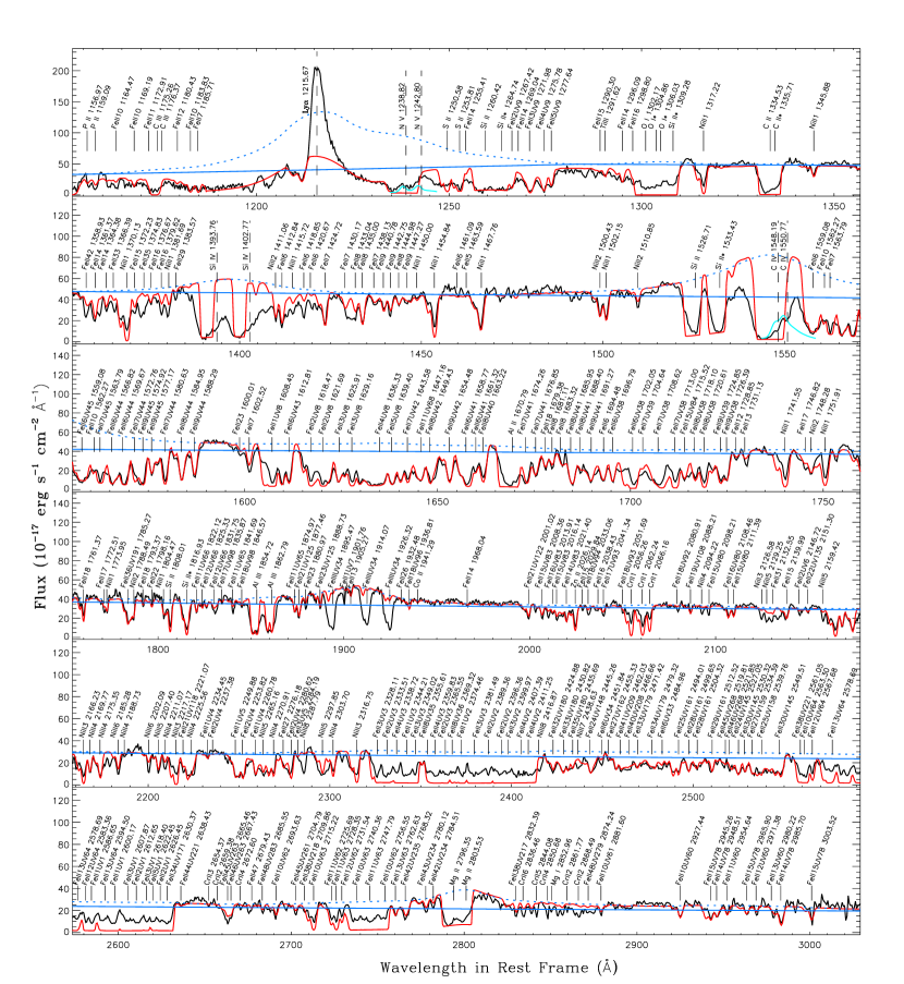
Figure 7: The synthetic spectrum of photoionization modeling. The red line represents the synthetic absorption spectrum constructed from Cloudy model based on a continuous stratified medium. The synthetic emission spectra of the strong resonnace doublets, C IV $\lambda\lambda 1548,1550$ and N V $\lambda\lambda 1238,1242$ predicted by Cloudy model are drawn in solid cyan lines superimposed on the residual intensities due to partial covering effects at the bottom of the absorption lines. The gray long-dashed vertical lines correspond to the rest-frame wavelength of each emission line.

6.2 Geometrical Configuration of the Absorber

Here, we estimated the position and radial range of the UV absorber in SDSS J0839+3805. The location of the intrinsic absorber (defined by distance $R_{\rm{abs}}$) with respect to the central source can be constrained by the ionization parameter, ($U=Q_{\rm H}/4\pi R_{\rm{abs}}^{2}n_{\mathrm{H}}c$), which gives the ratio of number densities between hydrogen ionizing photons ($Q_{\rm H}$) at the face of the absorber and hydrogen in all forms ($n_{\mathrm{H}}$). Here, $c$ is the speed of light. The value of $Q_{\rm H}$ can be evaluated using the SED of the ionizing continuum. Based on Cloudy models, the distance $R_{\mathrm{abs}}$ as a function of $U$, $n_{\mathrm{H}}$ and $Q_{\rm H}$ can be easily derived. Our uniform density model yields a radial distance of $R_{\mathrm{abs}}\approx$ 32 pc from the nucleus to the absorbing clouds. Furthermore, the revised two-component model can refine constraints on the radial span of the absorber and on $R_{\rm{abs}}$. We can place a lower limit on the radial thickness of a contiguous absorber in our Cloudy model using $\Delta{R}\sim N_{\rm H}/n_{\rm H}$.

The final solution of model #19-1 yields a radial span of the absorber $\sim$ 1.3 pc, originating at a radial distance of $R_{\mathrm{abs}}$ = 22.7 pc. From the model group with metallicities, Z = 0.8/0.5 Z_⊙, listed in Table  3, we conservatively estimated $R_{\rm{abs}}$ and the radial span of the absorber as $22.7^{+2.7}_{-2.5}$ pc, and 1.3$\sim$2.6 pc, respectively.

To estimate the relative position of the absorber among nuclear environments, we constrained the other characteristic sizes of the object. Using the $R_{\rm BLR}$–$L$ relationship (see equation (2) of Bentz et al., 2009), we can estimate the size of BLR. We measured an extinction-corrected luminosity at 5100 Å for an extinction, $E(B-V)=0.03$, which gives $\lambda L_{\lambda}(5100)=1.90\times 10^{46}\hbox{~{}erg~{}s}^{-1}$ that corresponds to a BLR of size, $R_{\rm{BLR}}$ = 0.44 pc.

The dust sublimation radius which can act as the inner edge of the torus is given by $R_{\rm{sub}}=1.3L^{1/2}_{uv,46}T^{-2.8}_{1500}$ pc (see equation (5) of Barvainis, 1987). Here, $L_{uv,46}$ is the total ultraviolet luminosity in units of $10^{46}\hbox{~{}erg~{}s}^{-1}$ and $T_{1500}$ is the grain evaporation temperature in units of 1500 K. For SDSS J0839+3805, assuming a dust temperature of 1500 K, we obtained $R_{\rm{sub}}\approx$ 2.6 pc using the model result $L_{uv,46}$ = 4.02. These values can be used to estimate the torus size which is usually 5-10 times larger than $R_{\rm{sub}}$ (Elitzur & Shlosman, 2006).

We roughly measured the FWHMs of the Ly$\alpha$ emission in the DLA trough and the broad H$\alpha$ emission as $\sim 897$ and $6700\hbox{~{}km~{}s${}^{-1}$}$, respectively. Assuming that the Ly$\alpha$ emitter is similar to the BLR, $R_{\rm{BLR}}\propto\rm{FWHM_{BLR}}^{2}$ and using the FWHMs of the Ly$\alpha$ and H$\alpha$ (which represent BLR emission), we found that the Ly$\alpha$ emitter is about (6700/897)² times farther than the BLR which locates at a distance of $R_{\rm{Ly\alpha}}\approx$ 24.5 pc from the nucleus. This is consistent with the result $\sim$21.5 pc estimated by means of the measurements of Ly$\alpha$ and H$\alpha$ made by Aoki et al. (2006) within uncertainty of 0.1 dex between the two measure. The FWHMs of Ly$\alpha$ and H$\alpha$ are $930\pm 25$ and $6500\pm 50$, respectively (see Table  2 of Aoki et al., 2006). The similar distance of the Ly$\alpha$ emitter and the UV absorber, $R_{\mathrm{abs}}$ from the nucleus suggests that the DLA absorber is also responsible for the Ly$\alpha$ emission. This result is supported by the characteristics of Ly$\alpha$-like emissions (e.g., C IV, N V) predicted by our simulations, which align reasonably well with observations.

The observed Ly$\alpha$ emission exhibits a rest-frame EW of approximately 14.4 Å. In contrast, the predicted Ly$\alpha$ EW, assuming complete absorption of the ionizing continuum radiation by optically thick BLR clouds (Peterson, 1997), is approximately 580 Å. This yield a global covering factor of the Ly$\alpha$ emitter to be around 2.5%, which means that an optically thick cloud would absorb about 2.5% of the ionizing continuum photons and create an equal amount of Ly$\alpha$ photons via recombination (Kwan & Krolik, 1979; Osterbrock & Ferland, 2006) towards our line of sight. This covering factor corresponds to a toroidal structure of scale height $\sim$ 1.2 pc that is located at a distance of $\sim$ 23 pc from the nucleus. Half of the scale height can therefore be used to set an upper limit on the vertical thickness of the absorbing gas. This is consistent with values estimated based on partial coverage analysis. The partial coverage of the BLR indicates that the absorber has a size that is comparable to, or less than the largest projected size of the BLR.

7 Summary and Discussion

In our study, we have discovered a strong DLA absorber that is roughly cospatial with the dusty torus in the quasar SDSS J0839+3805 located at redshift, $z=2.315$. Additionally, we have identified an exceptionally intense Ly$\alpha$ emission with a rest EW $\sim 14.4\pm 1.1$ Å and a $\mathrm{FWHM}\sim 897\pm 69\hbox{~{}km~{}s${}^{-1}$}$, intermediate between the characteristics of classic broad and narrow emission lines. This absorber is nearly dust-free and acts as a natural coronagraph and manifests itself in both absorption- and emission-lines. Extensive photoionization modeling reveals a turbulent, near-solar metallicity absorber, where the main characteristic of the quasar spectrum can be successfuly reproduced by a two component model.

Our model consists of a diffuse lower density H II-zone with $\log\,U=0.9$, $\log\,n_{\mathrm{H}}(\mathrm{cm}^{-3})=4.8$, $\log\,N_{\mathrm{H}}(\mathrm{cm}^{-2})=23.4$, and Z = 0.8Z_⊙, followed by a denser H I*-zone behind it with $\log\,n_{\mathrm{H}}(\mathrm{cm}^{-3})=6.6$, $\log\ N_{\mathrm{H\,\textsc{i}}}=21.9$, and Z = 0.5Z_⊙ with turbulent velocity, $v=100\hbox{~{}km~{}s${}^{-1}$}$. This absorber has a toroidal structure which is roughly collocated with the dusty torus and it has an upper limit of $\sim 0.6$ pc on its vertical thickness. The conclusive results are grounded in the following pieces of evidence:

1. DLAs with partial coverage: The residual intensity in the DLA trough, influenced by partial covering from the BLR, is determined by the covering factor measured using the residual intensity at the lowest points of the representative absorption lines of C II $\lambda 1334$, Si II $\lambda 1526$, C IV $\lambda 1548$, and Mg II $\lambda 2796$ which are expected to be completely saturated. In any case, partial coverage can constrain the relative sizes of the absorbers and nuclear emission sources, placing a lower limit on the transverse size of the absorber.

2. Non-negligible global covering factor: The observed rest EW of $\sim$ 14.4 Å of the Ly$\alpha$ emission yields a global covering factor of the Ly$\alpha$ emitter to be around 2.5%. This covering factor corresponds to a toroidal structure of scale height $\sim$ 1.2 pc that is located at a distance of $\sim$ 23 pc from the nucleus. Half of the scale height can be regarded as the vertical thickness of the absorbing gas which is consistent with estimates from partial coverage analysis.

3. Axisymmetric and self-shielding clouds: The extracted Ly$\alpha$ emission, which has skewed and redshifted wing (from $\sim-500$ to 1500 km s^-1), contrary to blueshifted BAL troughs (from $\sim$ 500 to $-1500\hbox{~{}km~{}s${}^{-1}$}$) which extends to the similar velocity width, suggests an axisymmetric and self-shielding clouds. This is reinforced by the lack of spectral variability, which indicates that the cloud is either far from the source or is being continually replenished, and is azimuthally symmetric (Gibson et al., 2008).

4. Collocated with the dusty torus: The location of the Ly$\alpha$ emitter ($R_{\rm{Ly\alpha}}\approx$ 21.5$-$24.5 pc), derived from the widths of the Ly$\alpha$ and H$\alpha$ emissions, is consistent with that of the DLA absorber (located at $R_{\rm{abs}}=22.7$ pc with a radial span of 1.3$\sim$2.6 pc), indicating a shared origin of them from a region that is collocated with the dusty torus.

5. Prediction of emission-line ratios: The photoionization model of the DLA absorber gives emission-line ratios that are close to the observed values of the broad emission lines (C IV/Ly$\alpha$$\sim$ 0.08$-$0.14, N V/Ly$\alpha$$\sim$ 0.2).

6. The emission-line ratios suggest an intrinsic origin: The line ratios of C IV/Ly$\alpha$ and N V/Ly$\alpha$, either measured from the observed spectrum or predicted by our models, are consistent with the mean ratios of C IV/Ly$\alpha$= 0.21 $\pm$ 0.09 that were measured for four local Seyfert 2 galaxies by Ferland & Osterbrock (1986) and N V/Ly$\alpha$ ranging from 0.03 to 0.3 measured in most Seyfert 2 galaxies (see Dey et al., 1998). In contrast, the non-AGN spectrum has intensity ratios of C IV/Ly$\alpha$ less or equal to 0.02 (see Shapley et al., 2003). This is also consistent with the finding of Francis et al. (1992) that the BAL QSOs show excess N V emission relative to the QSO population as a whole.

Taking all these points into account, we conclude that the DLA absorber that is causing the absorptions is also responsible for the Ly$\alpha$-like emissions, and is collocated with the dusty torus. If the gas lies along our line of sight to the nucleus, the absorption is observed; if the gas lies out of our line of sight, but still within instrumental angular resolution, only the emission which is attributed to the reprocessing of the central continuum radiation can be detected. The most plausible scenario is that the dusty torus is inherently geometrically thick, likely a consequence of gas inflow from galactic scales to the black hole, propelled by gravitational torques during its gas-rich phase (Hopkins et al., 2012). Thus, this torus can serves as a fuel reservoir, establishing a connection between the outer accretion disk and its host galaxy, thereby regulating the fueling from the torus through a dust and gas flow cycle. The evaporative absorber (outflow) is being continually replenished in a toroidal structure that can support a geometrically thick long-lived torus with internal turbulence by interacting with inflow (Dorodnitsyn et al., 2011; Wada, 2012).

Although the synthetic spectra constructed using the code CLOUDY successfully fit the observations as a whole, there exist some obvious discrepancies such as: significant residuals in absorption troughs of Fe II multiplets UV 1, UV 2, UV 3, UV 62 and 63 near 2600 Å, 2382 Å, 2344 Å, and 2750 Å; the observed absorptions of Fe III UV 34 triplet are much stronger than predictions from Cloudy photoionization simulations, etc. The predicted Fe II emissions from the absorber in the photoionization calculations are much less than the residual fluxes of Fe II (not shown in Fig. 7). If the residual fluxes are due to Fe II emission from the BLR leaking through the absorber with covering factor similar to those of Mg II ($\sim$0.74), then such high covering factor would result in too strong broad Fe II emission to credible. The photoionization models of the BLR in quasars still struggle to account for the observed intensities of Fe II. Our study implies that the strong Fe II emission emitted from outside of the BLR. This result is consistent with the finding of Popović et al. (2009) that the location of the Fe II emission region is located outside the BLR (the so-called intermediate line region or ILR), which was confirmed by Fe II reverberation (Barth et al., 2013). Fe III UV 34 absorptions are another problem. The unusual prominent three absorption lines $\lambda\lambda 1895.5,1914.1,1926.3$ are Fe III absorption by the triplet UV 34 from a low-lying metastable level at 3.73 eV. A possible population mechanism for Fe III UV 34 is that the upper level of Fe III UV 34 is populated by Ly$\alpha$ pumping (Johansson et al., 2000), and subsequent cascade to low-lying metastable levels. But in reality the population mechanism for Fe III UV 34 absorptions cannot be considered solved, and may not be well handled in code Cloudy, leading to a much lower Fe III UV 34 absorptions predicted by Cloudy simulations. Other explanations for these discrepancies are: the lines missing from the atomic line list or the available atomic data are likely inaccurate, and the model could be still simplified for the actual physical conditions of the absorber, especially for high-ionization lines, etc.

This object is viewed nearly edge-on and exhibits partial coverage to the BLR, thus there is a high possibility that it is viewed through the disk wind, across the BLR clouds, as well as infalling gas near and likely originated inside the dust sublimation radius. The influence of all the flows on the line absorption profile are neglected in this paper.

Finally, we provide a concise discussion on the limitations of absorption line analysis based on low-resolution spectra. Our confidence in the absorption line measurements is supported by the following reasons:

1. The predicted population of H$\alpha$ is consistent with the value derived by Aoki et al. (2006) where they used the curve of growth which was developed to deal with low-resolution data (Jenkins, 1986).

2. For quasars having high-quality and low-resolution data, as for example SDSS J170542.91+354340.2, absorption line measurements from low-resolution SDSS (R $\sim$ 2000) data and high-resolution VLT/UVES (R $\sim$ 50000) data yield very close column densities, with deviations within the predicted measurement uncertainties of  0.1 dex (see Table  4 of Pan et al., 2017).

3. For SDSS J0839+3805, over 200 absorption lines can be verified, including some very common multiplets like Fe II. The fitted profiles for low-ionization lines such as Ni II $\lambda 1455$ give FWHM of (225 $\pm 13)\hbox{~{}km~{}s${}^{-1}$}$, and (252 $\pm 60)\hbox{~{}km~{}s${}^{-1}$}$ with deconvolved FWHMs of 168  km s^-1and 204  km s^-1(applying the average resolution R $\sim$ 2000), respectively. The line profiles are marginally resolved and have similar wide low-ionization absorptions to those of SDSS J170542.91+354340.2.

Thus, absorption line measurements can be conducted reliably, with conservative uncertainties of $\sim$0.2 dex, even when the data resolution is low.

Data Availability

The spectroscopic data underlying this article are publicly available in SDSS data bases. The atomic data of Fe II for four datasets are publicly available in the release of CLOUDY. The derived data generated in this research will be shared on reasonable request to the first author.

Appendix A A comparison of atomic data for selected lines of Fe II for four datasets.

In this study, we have used the oscillator strengths (f-values) for a number of Fe II lines for four datasets from Verner et al. (1999), Smyth et al. (2019), Tayal & Zatsarinny (2018) and CHIANTI (Version 10.1) that are in the release of CLOUDY. Comparisons among the four datasets reveal large discrepancies in transition probabilities or oscillator strengths for part of transitions. The adoption of the most reliable f-values (and atomic data in general) can often significantly affect the photoionization modeling results. There is still a pressing need for improvements in highly reliable sets of atomic data for Fe II.

We also observed a discrepancy in the total angular momentum (J) value for the same level between Tayal & Zatsarinny (2018) and the other three datasets, which consequently impacts the deduced oscillator strength of the corresponding transitions. The results are listed in Table 4. The index of the level ($\geq$ 114) contained in the Verner99 term, minus the number in parentheses, represents the modified level number that aligns with the atomic data for Fe II in Verner et al. (1999).

Table 5 list a comparison of atomic data for selected lines of Fe II from four datasets. Wavelengths, index of the lower (l) and upper levels (u), and statistical weights (i.e. degeneracy) of lower and upper levels from Verner et al. (1999) are given in columns 1 to 5, respectively. Transition probabilities (Einstein A coefficient) and then the deduced oscillator strengths (f-values) are included for four datasets, if they exist. The data denoted by * in the list were used to replace the counterpart of Verner et al. (1999) to produce synthetic Fe II spectra.The Einstein A coefficient for spontaneous decay is related to the absorption oscillator strength of the upward transition by

$$A_{\rm ul}=\frac{8\pi^{2}e^{2}\nu^{2}}{m_{e}c^{3}}\frac{g_{l}}{g_{u}}f_{lu}=\frac{8\pi^{2}e^{2}}{m_{e}c\lambda^{2}}\frac{g_{l}}{g_{u}}f_{lu},$$ (5)

$m_{e}$ is electron mass.

Table 4: Comparison of the disparity of the total angular momentum (J) value of the same level between Tayal & Zatsarinny (2018) and other three datasets. Energies are the data of four Fe II data sets that are incorporated into the CLOUDY modelling code.

Configuration	Term	Tayal18				Smyth19				Verner99				CHIANTI
		Index	J	Energy (cm${}^{-1})$		Index	J	Energy (cm${}^{-1})$		Index	J	Energy (cm${}^{-1})$		Index	J	Energy (cm${}^{-1})$
$3d^{6}(^{3}D)4s$	${}^{4}D$	49	$1/2$	31364.5		49	$3/2$	31364.4457		49	$3/2$	31364.440		34	$3/2$	31364.439
		50	$3/2$	31368.5		50	$1/2$	31368.4511		50	$1/2$	31368.450		35	$1/2$	31368.449
$3d^{6}(^{1}F)4s$	${}^{2}F$	82	$5/2$	44915.1		82	$7/2$	44915.0489		82	$7/2$	44915.046
		83	$7/2$	44929.5		83	$5/2$	44929.5233		83	$5/2$	44929.550
$3d^{6}(^{3}F)4s$	${}^{4}F$	97	$7/2$	50157.5		97	$9/2$	50157.4631		97	$9/2$	50157.452		61	$9/2$	50157.453
		98	$9/2$	50187.8		98	$7/2$	50187.8164		98	$7/2$	50187.813		62	$7/2$	50187.812
$3d^{6}(^{3}G)4p$	${}^{4}G$	159	$5/2$	64040.9		157	$7/2$	64040.8776		159(1)	$7/2$	64040.886		98	$7/2$	64040.887
		160	$7/2$	64087.4		158	$5/2$	64087.3953		160(1)	$5/2$	64087.418		99	$5/2$	64087.418
$3d^{6}(^{3}G)4p$	${}^{4}H$	179	$7/2$	66589.0		177	$9/2$	66589.0326		179(1)	$9/2$	66589.008		110	$9/2$	66589.008
		181	$9/2$	66672.3		179	$7/2$	66672.3232		181(1)	$7/2$	66672.334		111	$7/2$	66672.336
$3d^{6}(^{1}G)4p$	${}^{2}H$	184	$9/2$	67516.3		182	$11/2$	67516.3237		184(1)	$11/2$	67516.332
		185	$11/2$	68000.8		186	$9/2$	68000.7700		185(1)	$9/2$	68000.788
$3d^{5}4s^{2}$	${}^{2}G$	242	$9/2$	78185.0		239	$7/2$	78184.9950		232(2)	$7/2$	78185.030
		248	$7/2$	78577.3		243	$9/2$	78577.2510		236(2)	$9/2$	78577.280
$3d^{6}(^{3}D)4p$	${}^{2}P$	252	$3/2$	78841.9		246	$1/2$	78841.8606		239(2)	$1/2$	78841.960
		254	$1/2$	79243.5		248	$3/2$	79243.4552		241(2)	$3/2$	79243.600
$3d^{6}(^{3}F)4p$	${}^{4}D$	310	$7/2$	92899.3						366(2)	$5/2$	92899.200
		311	$5/2$	93129.9		393	$7/2$	93129.8655		367(2)	$7/2$	93129.900

Table 5: Comparison of atomic data for selected lines of Fe II for four datasets. The Fe II data sets of Verner et al. (1999), Smyth et al. (2019), Tayal & Zatsarinny (2018) and CHIANTI that are in the release of CLOUDY.

Wavelength	$I_{\rm l}$	$I_{\rm u}$	$g_{\rm l}$	$g_{\rm u}$	Verner99			Smyth19				Tayal18				CHIANTI
					$A_{\rm ul}$	$f_{\rm v}$		$A_{\rm ul}$	$f_{\rm s}$	$f_{\rm s}/f_{\rm v}$		$A_{\rm ul}$	$f_{\rm t}$	$f_{\rm t}/f_{\rm v}$		$A_{\rm ul}$	$f_{\rm c}$	$f_{\rm c}/f_{\rm v}$
2600.1729	1	64	10	10	2.39e+08	2.42e-01		2.53e+08	2.56e-01	1.06e+00		2.75e+08	2.79e-01	1.15e+00		2.37e+08	2.40e-01	9.92e-01
2586.6499	1	65	10	8	8.84e+07	7.09e-02		8.76e+07	7.03e-02	9.92e-01		1.00e+08	8.02e-02	1.13e+00		6.83e+07	5.48e-02	7.73e-01
2382.7651	1	69	10	12	3.36e+08	3.43e-01		3.40e+08	3.47e-01	1.01e+00		3.88e+08	3.96e-01	1.15e+00		3.35e+08	3.42e-01	9.97e-01
2374.4612	1	70	10	10	3.90e+07	3.30e-02		4.69e+07	3.96e-02	1.20e+00		4.80e+07	4.06e-02	1.23e+00		6.24e+07	5.27e-02	1.60e+00
2367.5906	1	71	10	8	3.21e+04	2.16e-05		8.41e+06	5.65e-03	2.62e+02		4.96e+05	3.33e-04	1.54e+01		6.32e+06	4.25e-03	1.97e+02
2344.2139	1	75	10	8	1.90e+08	1.25e-01		1.79e+08	1.18e-01	9.44e-01		2.27e+08	1.50e-01	1.20e+00		1.92e+08	1.26e-01	1.01e+00
2260.7805	1	78	10	10	3.42e+06	2.62e-03		1.41e+06	1.08e-03*	4.12e-01		3.02e+06	2.31e-03	8.82e-01
2234.4473	1	80	10	8	4.22e+04	2.53e-05		2.67e+05	1.60e-04*	6.32e+00		3.17e+04	1.90e-05	7.51e-01
2612.6543	2	65	8	8	1.22e+08	1.25e-01		1.31e+08	1.34e-01	1.07e+00		1.41e+08	1.44e-01	1.15e+00		1.28e+08	1.31e-01	1.05e+00
2599.1465	2	66	8	6	1.43e+08	1.09e-01		1.46e+08	1.11e-01	1.02e+00		1.63e+08	1.24e-01	1.14e+00		1.25e+08	9.48e-02	8.70e-01
2396.3560	2	70	8	10	2.86e+08	3.08e-01		2.87e+08	3.09e-01	1.00e+00		3.29e+08	3.54e-01	1.15e+00		2.68e+08	2.89e-01	9.38e-01
2389.3582	2	71	8	8	1.05e+08	8.99e-02		1.47e+08	1.26e-01	1.40e+00		1.19e+08	1.02e-01	1.13e+00		1.13e+08	9.68e-02	1.08e+00
2365.5518	2	75	8	8	6.30e+07	5.29e-02		2.04e+07	1.71e-02	3.23e-01		7.79e+07	6.54e-02	1.24e+00		5.35e+07	4.49e-02	8.49e-01
2333.5156	2	76	8	6	1.27e+08	7.78e-02		1.25e+08	7.65e-02	9.83e-01		1.51e+08	9.25e-02	1.19e+00		1.33e+08	8.14e-02	1.05e+00
2280.6201	2	78	8	10	5.26e+06	5.13e-03		7.90e+05	7.70e-04	1.50e-01		4.61e+06	4.49e-03*	8.75e-01
2253.8254	2	80	8	8	4.23e+06	3.22e-03		7.03e+05	5.35e-04	1.66e-01		3.71e+06	2.83e-03*	8.79e-01
2632.1082	3	65	6	8	5.95e+07	8.24e-02		7.31e+07	1.01e-01	1.23e+00		7.19e+07	9.96e-02	1.21e+00		9.01e+07	1.25e-01	1.52e+00
2607.8665	3	67	6	4	1.81e+08	1.23e-01		1.90e+08	1.29e-01	1.05e+00		2.08e+08	1.41e-01	1.15e+00		1.73e+08	1.18e-01	9.59e-01
2405.6187	3	71	6	8	2.17e+08	2.51e-01		1.67e+08	1.93e-01	7.69e-01		2.54e+08	2.94e-01	1.17e+00		2.10e+08	2.43e-01	9.68e-01
2399.9729	3	72	6	6	1.45e+08	1.25e-01		1.52e+08	1.31e-01	1.05e+00		1.67e+08	1.44e-01	1.15e+00		1.52e+08	1.31e-01	1.05e+00
2381.4888	3	75	6	8	3.35e+07	3.80e-02		8.08e+07	9.16e-02	2.41e+00		3.21e+07	3.64e-02	9.58e-01		8.72e+06	9.88e-03	2.60e-01
2349.0222	3	76	6	6	1.08e+08	8.93e-02		1.00e+08	8.27e-02	9.26e-01		1.29e+08	1.07e-01	1.20e+00		9.32e+07	7.71e-02	8.63e-01
2284.1899	3	79	6	8	7.76e+04	8.09e-05		4.58e+05	4.78e-04*	5.91e+00		4.61e+03	4.81e-06	5.95e-02
2268.2878	3	80	6	8	3.90e+06	4.01e-03		3.70e+05	3.81e-04	9.50e-02		3.54e+06	3.64e-03*	9.08e-01
2360.7207	6	78	10	10	2.74e+07	2.29e-02		7.45e+07	6.22e-02	2.72e+00		2.60e+07	2.17e-02	9.48e-01		4.74e+07	3.96e-02	1.73e+00
2348.8342	6	79	10	8	5.52e+07	3.65e-02		2.17e+08	1.44e-01	3.95e+00		5.52e+07	3.65e-02	1.00e+00		1.30e+08	8.60e-02	2.36e+00
2332.0227	6	80	10	8	2.74e+07	1.79e-02		4.03e+06	2.63e-03	1.47e-01		2.83e+07	1.85e-02	1.03e+00		5.56e+06	3.63e-03	2.03e-01
1696.7943	6	122	10	10	1.74e+07	7.51e-03		3.16e+04	1.36e-05	1.81e-03		3.17e+07	1.37e-02	1.82e+00		1.33e+07	5.74e-03*	7.64e-01
1694.4836	6	124	10	12	7.87e+05	4.07e-04						6.99e+06	3.61e-03*	8.87e+00
1661.3240	6	139	10	8	1.25e+06	4.14e-04		2.94e+05	9.73e-05	2.35e-01		1.62e+06	5.36e-04	1.29e+00		4.97e+06	1.65e-03*	3.99e+00
1637.3990	6	151	10	8	4.41e+07	1.42e-02		4.18e+08	1.34e-01	9.44e+00		6.23e+07	2.00e-02	1.41e+00		2.38e+07	7.65e-03*	5.39e-01
1612.8057	6	156	10	12	6.57e+07	3.07e-02		2.50e+07	1.17e-02	3.81e-01		6.02e+05	2.82e-04	9.19e-03		2.13e+07	9.97e-03*	3.25e-01
1602.2103	6	160	10	8	1.05e+06	3.23e-04		3.41e+07	1.05e-02	3.25e+01		5.78e+05	1.78e-04	5.51e-01
1569.6746	6	168	10	12	2.30e+07	1.02e-02		1.56e+08	6.91e-02	6.77e+00		3.82e+06	1.69e-03	1.66e-01		4.22e+07	1.87e-02	1.83e+00
1566.8217	6	169	10	10	5.20e+07	1.91e-02		1.67e+07	6.15e-03	3.22e-01		4.89e+04	1.80e-05	9.42e-04		3.51e+06	1.29e-03	6.75e-02
2344.6780	7	85	8	6	2.70e+07	1.67e-02		9.67e+05	5.98e-04	3.58e-02		2.89e+07	1.79e-02	1.07e+00		9.42e+06	5.82e-03	3.49e-01
1676.8557	7	139	8	8	6.82e+06	2.87e-03		2.14e+07	9.02e-03	3.14e+00		9.65e+06	4.07e-03*	1.42e+00		3.56e+07	1.50e-02	5.23e+00
1676.3613	7	140	8	10	1.32e+06	6.95e-04		2.07e+08	1.09e-01	1.57e+02		4.47e+06	2.35e-03*	3.38e+00
1674.4399	7	142	8	6	1.41e+06	4.45e-04		1.49e+04	4.70e-06	1.06e-02		3.90e+05	1.23e-04	2.76e-01		8.37e+06	2.64e-03*	5.93e+00
1674.2563	7	143	8	10	1.08e+07	5.67e-03		5.19e+06	2.73e-03	4.81e-01		2.37e+07	1.24e-02	2.19e+00		3.89e+06	2.04e-03*	3.60e-01
1625.5222	7	157	8	10	5.01e+07	2.48e-02		2.12e+07	1.05e-02	4.23e-01		7.24e+05	3.59e-04	1.45e-02		1.91e+07	9.46e-03*	3.81e-01
1602.5167	7	163	8	10	2.23e+06	1.07e-03		7.61e+06	3.66e-03*	3.42e+00		5.07e+05	2.44e-04	2.28e-01
1580.6293	7	169	8	10	5.79e+07	2.71e-02		1.33e+08	6.23e-02	2.30e+00		9.18e+06	4.30e-03	1.59e-01		3.78e+07	1.77e-02*	6.53e-01
1572.7560	7	171	8	10	8.56e+05	3.97e-04		6.48e+07	3.00e-02	7.56e+01		2.05e+07	9.50e-03*	2.39e+01		2.16e+07	1.00e-02	2.52e+01
1560.2521	7	177	8	6	1.96e+07	5.36e-03		5.06e+07	1.39e-02	2.59e+00		1.75e+07	4.79e-03	8.94e-01		4.76e+07	1.30e-02*	2.43e+00
1430.1665	7	201	8	8	1.00e+06	3.07e-04		6.65e+06	2.04e-03*	6.64e+00		5.55e+06	1.70e-03	5.54e+00		1.73e+06	5.29e-04	1.72e+00
1424.7167	7	204	8	6	1.97e+07	4.50e-03		4.90e+07	1.12e-02	2.49e+00		3.14e+07	7.17e-03	1.59e+00		3.11e+07	7.10e-03*	1.58e+00
1185.7124	7	291	8	6	1.78e+07	2.81e-03		3.24e+07	5.12e-03*	1.82e+00		8.40e+06	1.33e-03	4.73e-01		3.12e+07	4.93e-03	1.75e+00
1720.6127	8	125	6	8	5.88e+07	3.48e-02		6.92e+03	4.10e-06	1.18e-04		7.21e+07	4.27e-02	1.23e+00		1.32e+08	7.82e-02	2.25e+00
1718.1010	8	128	6	6	1.41e+07	6.24e-03		3.77e+07	1.67e-02	2.68e+00		4.65e+07	2.06e-02	3.30e+00		2.13e+07	9.43e-03	1.51e+00
1698.1353	8	136	6	8	1.39e+06	8.01e-04		7.71e+05	4.44e-04	5.54e-01		3.68e+06	2.12e-03*	2.65e+00		5.74e+05	3.31e-04	4.13e-01
1688.4030	8	139	6	8	3.67e+06	2.09e-03		6.00e+06	3.42e-03	1.64e+00		2.00e+07	1.14e-02	5.45e+00		6.13e+06	3.49e-03*	1.67e+00
1683.3156	8	145	6	4	2.69e+05	7.62e-05		2.76e+06	7.82e-04	1.03e+01		8.41e+06	2.38e-03	3.12e+01		9.23e+06	2.61e-03*	3.43e+01
1681.1107	8	147	6	8	6.47e+06	3.66e-03		1.88e+08	1.06e-01	2.90e+01		7.33e+06	4.14e-03*	1.13e+00
1654.6696	8	153	6	6	9.00e+05	3.69e-04		4.48e+07	1.84e-02	4.99e+01		2.22e+06	9.11e-04	2.47e+00		4.50e+06	1.85e-03*	5.01e+00
1584.9521	8	170	6	8	5.80e+07	2.91e-02		1.34e+08	6.73e-02	2.31e+00		9.50e+06	4.77e-03	1.64e-01		3.52e+07	1.77e-02*	6.08e-01
1444.9807	8	195	6	4	3.59e+06	7.49e-04		9.80e+06	2.05e-03*	2.74e+00		3.87e+05	8.08e-05	1.08e-01
1440.9105	8	199	6	6	7.34e+05	2.28e-04		5.92e+06	1.84e-03*	8.07e+00		5.39e+06	1.68e-03	7.37e+00		1.52e+06	4.74e-04	2.08e+00
1434.9958	8	203	6	4	1.89e+07	3.89e-03		4.99e+07	1.03e-02*	2.65e+00		3.30e+07	6.79e-03	1.75e+00		3.00e+07	6.17e-03	1.59e+00
1433.0438	8	204	6	6	2.85e+06	8.77e-04		6.75e+06	2.08e-03*	2.37e+00		3.56e+06	1.10e-03	1.25e+00		6.51e+06	2.00e-03	2.28e+00
1726.3916	9	128	4	6	3.23e+07	2.16e-02		1.74e+08	1.17e-01	5.42e+00		1.29e+08	8.65e-02	4.00e+00		1.30e+08	8.73e-02	4.04e+00
1691.2729	9	145	4	4	2.56e+07	1.10e-02		1.85e+07	7.93e-03	7.21e-01		4.13e+07	1.77e-02	1.61e+00		3.64e+07	1.56e-02*	1.42e+00
1674.7161	9	150	4	2	9.12e+07	1.92e-02		7.19e+06	1.51e-03	7.86e-02		4.74e+07	9.97e-03	5.19e-01		1.16e+08	2.43e-02	1.27e+00
1654.4779	9	155	4	2	7.15e+07	1.47e-02		5.06e+08	1.04e-01	7.07e+00		1.24e+08	2.54e-02*	1.73e+00		2.59e+07	5.31e-03	3.61e-01
1640.1521	9	159	4	6	5.90e+07	3.57e-02		1.92e+07	1.16e-02	3.25e-01						1.74e+07	1.05e-02*	2.94e-01
1588.2897	9	172	4	6	4.82e+07	2.73e-02		1.31e+08	7.43e-02	2.72e+00		1.33e+07	7.55e-03	2.77e-01		3.49e+07	1.98e-02*	7.25e-01
1577.1666	9	177	4	6	1.69e+07	9.45e-03		9.16e+07	5.12e-02	5.42e+00		2.86e+07	1.60e-02	1.69e+00		3.44e+07	1.93e-02*	2.04e+00
1574.9222	9	179	4	4	1.21e+08	4.50e-02		4.47e+08	1.66e-01	3.69e+00		1.23e+08	4.57e-02	1.02e+00		2.08e+08	7.72e-02	1.72e+00
1448.1937	9	197	4	4	1.15e+05	3.62e-05		5.31e+06	1.67e-03*	4.61e+01		5.09e+06	1.60e-03	4.42e+01		1.74e+06	5.49e-04	1.52e+01
1442.7465	9	202	4	2	1.81e+07	2.82e-03		4.00e+07	6.24e-03	2.21e+00		4.07e+07	6.35e-03*	2.25e+00		3.67e+07	5.73e-03	2.03e+00
1440.7747	9	203	4	4	3.75e+06	1.17e-03		9.84e+06	3.06e-03*	2.62e+00		5.35e+06	1.66e-03	1.42e+00		7.37e+06	2.29e-03	1.96e+00
2717.5020	10	80	8	8	7.35e+04	8.14e-05		1.06e+08	1.17e-01	1.44e+03		3.09e+05	3.42e-04	4.20e+00		3.51e+07	3.89e-02	4.78e+02
2715.2175	10	81	8	6	5.48e+07	4.54e-02		4.48e+07	3.71e-02	8.17e-01		6.74e+07	5.59e-02	1.23e+00		4.88e+07	4.04e-02	8.90e-01
2693.6333	10	85	8	6	1.59e+06	1.30e-03		1.59e+07	1.30e-02	1.00e+01		2.85e+06	2.33e-03*	1.79e+00		2.44e+06	1.99e-03	1.53e+00
2563.3042	10	88	8	6	1.83e+08	1.35e-01		1.95e+08	1.44e-01	1.07e+00		2.05e+08	1.51e-01	1.12e+00		1.93e+08	1.43e-01	1.06e+00
1722.4318	10	171	8	10	3.52e+06	1.96e-03		1.68e+07	9.34e-03*	4.77e+00		7.31e+06	4.06e-03	2.07e+00		7.33e+06	4.07e-03	2.08e+00
1183.8287	10	358	8	10	4.88e+07	1.28e-02		1.06e+08	2.78e-02*	2.17e+00		3.68e+07	9.66e-03	7.55e-01
1169.1902	10	368	8	10	3.91e+07	1.00e-02		5.57e+07	1.43e-02*	1.43e+00		3.11e+07	7.97e-03	7.97e-01		2.24e+05	5.73e-05	5.73e-03
2773.5447	11	79	6	8	1.07e+05	1.65e-04		1.16e+08	1.78e-01	1.08e+03		3.08e+05	4.74e-04	2.87e+00		3.43e+07	5.28e-02	3.20e+02
2728.3469	11	84	6	4	9.26e+07	6.89e-02		7.13e+07	5.30e-02*	7.69e-01		1.14e+08	8.48e-02	1.23e+00		8.86e+07	6.59e-02	9.56e-01
2725.6914	11	85	6	6	9.37e+06	1.04e-02		1.11e+08	1.24e-01	1.19e+01		8.60e+06	9.58e-03	9.21e-01		5.94e+07	6.61e-02	6.36e+00
1874.9717	11	136	6	8	2.13e+06	1.50e-03		7.81e+06	5.49e-03*	3.66e+00		1.91e+06	1.34e-03	8.93e-01		1.15e+06	8.05e-04	5.37e-01
1833.0764	11	151	6	8	2.23e+06	1.50e-03		1.71e+07	1.15e-02	7.67e+00		3.62e+06	2.43e-03*	1.62e+00		1.35e+06	9.04e-04	6.03e-01
1822.1230	11	153	6	6	4.26e+06	2.12e-03		9.84e+06	4.90e-03*	2.31e+00		7.62e+06	3.79e-03	1.79e+00		5.51e+06	2.74e-03	1.29e+00
1273.2739	11	292	6	8	1.18e+04	3.82e-06		2.21e+07	7.16e-03*	1.87e+03		3.98e+03	1.29e-06	3.38e-01		1.14e+05	3.70e-05	9.69e+00

Table 6: continued

Wavelength

$I_{\rm l}$

$I_{\rm u}$

$g_{\rm l}$

$g_{\rm u}$

Verner99

Smyth19

Tayal18

CHIANTI

$A_{\rm ul}$

$f_{\rm v}$

$A_{\rm ul}$

$f_{\rm s}$

$f_{\rm s}/f_{\rm v}$

$A_{\rm ul}$

$f_{\rm t}$

$f_{\rm t}/f_{\rm v}$

$A_{\rm ul}$

$f_{\rm c}$

$f_{\rm c}/f_{\rm v}$

2769.7527

12

81

4

6

3.87e+06

6.68e-03

1.31e+08

2.26e-01

3.38e+01

2.95e+06

5.09e-03

7.62e-01

5.64e+07

9.74e-02

1.46e+01

2731.5427

12

87

4

4

2.65e+07

2.96e-02

1.03e+08

1.15e-01

3.89e+00

2.74e+07

3.06e-02

1.03e+00

6.79e+07

7.60e-02

2.57e+00

1842.2397

12

152

4

4

3.00e+06

1.53e-03

3.87e+04

1.97e-05

1.29e-02

1.37e+06

6.97e-04

4.56e-01

3.39e+06

1.73e-03*

1.13e+00

1831.7527

12

153

4

6

3.07e+06

2.32e-03

8.63e+06

6.51e-03*

2.81e+00

6.18e+06

4.66e-03

2.01e+00

2.21e+06

1.67e-03

7.20e-01

1825.3286

12

154

4

4

3.75e+06

1.87e-03

1.40e+07

6.99e-03*

3.74e+00

6.86e+06

3.43e-03

1.83e+00

3.83e+06

1.91e-03

1.02e+00

1822.1895

12

155

4

2

6.25e+06

1.56e-03

2.18e+07

5.43e-03*

3.48e+00

1.10e+07

2.74e-03

1.76e+00

4.81e+06

1.20e-03

7.69e-01

1728.8521

12

177

4

6

3.20e+06

2.15e-03

8.71e+06

5.85e-03*

2.72e+00

4.21e+06

2.83e-03

1.32e+00

5.44e+06

3.65e-03

1.70e+00

1646.1847

12

187

4

2

1.38e+08

2.80e-02

2.40e+08

4.88e-02*

1.74e+00

1.22e+06

2.48e-04

8.86e-03

2762.6294

13

84

2

4

1.24e+07

2.84e-02

1.10e+08

2.52e-01

8.87e+00

1.12e+07

2.56e-02

9.01e-01

6.09e+07

1.39e-01

4.89e+00

2594.5042

13

89

2

4

1.43e+07

2.89e-02

1.24e+07

2.50e-02

8.65e-01

1.66e+07

3.35e-02

1.16e+00

1.16e+07

2.35e-02

8.13e-01

2578.6948

13

90

2

2

1.24e+08

1.24e-01

1.40e+08

1.40e-01

1.13e+00

1.41e+08

1.41e-01

1.14e+00

1.18e+08

1.18e-01

9.52e-01

1827.7285

13

155

2

2

6.59e+06

3.30e-03

2.30e+07

1.15e-02*

3.48e+00

1.10e+07

5.51e-03

1.67e+00

4.76e+06

2.39e-03

7.24e-01

1731.1255

13

179

2

4

3.27e+06

2.94e-03

9.40e+06

8.45e-03*

2.87e+00

4.21e+06

3.78e-03

1.29e+00

5.05e+06

4.54e-03

1.54e+00

1578.1282

13

198

2

2

9.53e+06

3.56e-03

6.47e+06

2.42e-03

6.80e-01

5.04e+06

1.88e-03

5.28e-01

8.58e+06

3.20e-03

8.99e-01

2985.6956

14

88

6

6

2.91e+07

3.89e-02

1.09e+08

1.46e-01

3.75e+00

2.83e+07

3.78e-02*

9.72e-01

4.38e+07

5.85e-02

1.50e+00

2948.5159

14

89

6

4

1.93e+07

1.68e-02

2.35e+07

2.04e-02*

1.21e+00

1.90e+07

1.65e-02

9.82e-01

2.92e+07

2.54e-02

1.51e+00

2165.0154

14

115

6

4

1.14e+07

5.34e-03

2.48e+07

1.16e-02

2.17e+00

1.68e+07

7.87e-03

1.47e+00

6.59e+07

3.09e-02

5.79e+00

2130.9270

14

118

6

6

3.87e+06

2.63e-03

9.48e+06

6.45e-03*

2.45e+00

2.43e+06

1.65e-03

6.27e-01

5.84e+07

3.98e-02

1.51e+01

2031.8815

14

149

6

6

2.24e+04

1.39e-05

1.59e+07

9.84e-03

7.08e+02

4.54e+06

2.81e-03

2.02e+02

2.86e+07

1.77e-02

1.27e+03

2021.4015

14

151

6

8

2.70e+07

2.21e-02

5.72e+06

4.67e-03

2.11e-01

2.93e+07

2.39e-02

1.08e+00

4.26e+07

3.48e-02*

1.57e+00

1693.4757

14

203

6

4

1.97e+07

5.65e-03

4.75e+07

1.36e-02*

2.41e+00

1.98e+06

5.68e-04

1.01e-01

2.46e+06

7.05e-04

1.25e-01

1690.7577

14

204

6

6

2.87e+07

1.23e-02

7.34e+07

3.15e-02*

2.56e+00

1.48e+07

6.34e-03

5.15e-01

1.48e+07

6.36e-03

5.17e-01

1689.8324

14

206

6

8

1.98e+07

1.13e-02

4.46e+07

2.55e-02

2.26e+00

2.12e+07

1.21e-02

1.07e+00

4.95e+07

2.83e-02*

2.50e+00

1364.3837

14

291

6

6

3.45e+07

9.63e-03

7.06e+07

1.97e-02*

2.05e+00

2.43e+07

6.78e-03

7.04e-01

3.18e+07

8.86e-03

9.20e-01

1296.0840

14

327

6

4

2.97e+06

4.99e-04

3.27e+08

5.49e-02*

1.10e+02

1.80e+08

3.02e-02

6.05e+01

2.32e+08

3.89e-02

7.80e+01

3003.5208

15

88

4

6

1.06e+07

2.15e-02

3.39e+07

6.88e-02

3.20e+00

1.02e+07

2.07e-02

9.63e-01

1.84e+07

3.74e-02*

1.74e+00

2965.8987

15

89

4

4

5.95e+06

7.85e-03

2.49e+07

3.28e-02

4.18e+00

5.87e+06

7.74e-03

9.86e-01

8.50e+06

1.12e-02*

1.43e+00

2945.2573

15

90

4

2

3.54e+07

2.30e-02

8.46e+07

5.50e-02

2.39e+00

3.47e+07

2.26e-02

9.83e-01

5.43e+07

3.53e-02*

1.53e+00

2174.3728

15

115

4

4

7.76e+05

5.50e-04

2.93e+06

2.08e-03

3.78e+00

5.70e+06

4.04e-03*

7.35e+00

4.34e+07

3.07e-02

5.58e+01

2139.9915

15

118

4

6

1.43e+05

1.47e-04

5.17e+05

5.32e-04

3.62e+00

8.57e+05

8.83e-04

6.01e+00

2.47e+07

2.55e-02*

1.73e+02

2111.3928

15

127

4

2

5.79e+06

1.93e-03

1.48e+07

4.95e-03

2.56e+00

3.32e+06

1.11e-03

5.75e-01

7.15e+07

2.39e-02*

1.24e+01

2016.1375

15

153

4

6

2.31e+07

2.11e-02

1.38e+06

1.26e-03

5.97e-02

2.24e+07

2.05e-02

9.72e-01

3.01e+07

2.75e-02*

1.30e+00

2008.3578

15

154

4

4

1.63e+07

9.86e-03

1.02e+07

6.17e-03

6.26e-01

1.48e+07

8.95e-03

9.08e-01

2.32e+07

1.40e-02*

1.42e+00

1715.5153

15

194

4

6

5.09e+07

3.37e-02

1.34e+08

8.87e-02*

2.63e+00

2.58e+07

1.71e-02

5.07e-01

3.47e+07

2.29e-02

6.80e-01

1372.2920

15

287

4

4

6.40e+07

1.81e-02

1.27e+08

3.59e-02*

1.98e+00

4.00e+07

1.13e-02

6.24e-01

5.55e+07

1.57e-02

8.67e-01

2986.4158

16

89

2

4

1.60e+07

4.28e-02

4.92e+07

1.32e-01

3.08e+00

1.55e+07

4.14e-02

9.67e-01

2.60e+07

6.96e-02

1.63e+00

2965.4890

16

90

2

2

6.54e+06

8.62e-03

1.50e+07

1.98e-02

2.30e+00

6.35e+06

8.37e-03

9.71e-01

1.06e+07

1.40e-02*

1.62e+00

2185.3799

16

115

2

4

4.09e+04

5.86e-05

3.57e+05

5.11e-04

8.72e+00

2.06e+06

2.95e-03

5.03e+01

2.14e+07

3.06e-02*

5.22e+02

2108.4619

16

131

2

4

1.45e+06

1.93e-03

4.37e+06

5.83e-03

3.02e+00

1.27e+06

1.69e-03

8.76e-01

3.59e+07

4.79e-02*

2.48e+01

2043.9761

16

150

2

2

2.85e+06

1.79e-03

6.59e+07

4.13e-02

2.31e+01

1.44e+07

9.02e-03*

5.04e+00

7.81e+07

4.89e-02

2.73e+01

2038.4292

16

152

2

4

4.93e+05

6.14e-04

3.25e+07

4.05e-02

6.60e+01

2.97e+06

3.70e-03*

6.03e+00

3.94e+07

4.90e-02

7.98e+01

2017.7448

16

154

2

4

1.49e+07

1.82e-02

3.86e+06

4.71e-03

2.59e-01

1.20e+07

1.46e-02

8.02e-01

1.78e+07

2.18e-02*

1.20e+00

2013.9095

16

155

2

2

2.75e+07

1.67e-02

1.63e+07

9.91e-03

5.93e-01

2.06e+07

1.25e-02

7.49e-01

3.59e+07

2.18e-02*

1.31e+00

1379.6149

16

284

2

2

1.01e+08

2.88e-02

2.01e+08

5.74e-02*

1.99e+00

5.97e+07

1.70e-02

5.90e-01

8.53e+07

2.43e-02

8.44e-01

1298.8018

16

332

2

4

3.78e+05

1.91e-04

7.56e+05

3.82e-04

2.00e+00

3.04e+07

1.54e-02*

8.06e+01

1935.2960

17

183

10

12

8.38e+06

5.65e-03

9.50e+07

6.40e-02

1.13e+01

1.05e+04

5.90e-06

1.04e-03

1936.8048

18

184

8

10

6.76e+06

4.75e-03

8.93e+07

6.28e-02*

1.32e+01

1761.3719

18

210

8

8

1.42e+08

6.60e-02

4.39e+08

2.04e-01*

3.09e+00

5.71e+06

2.66e-03

4.03e-02

2088.2051

19

173

4

2

1.37e+08

4.48e-02

3.81e+08

1.25e-01*

2.79e+00

1.24e+08

4.05e-02

9.04e-01

2001.0284

21

190

12

10

9.53e+07

4.77e-02

2.27e+08

1.14e-01*

2.39e+00

7.26e+06

3.63e-03

7.61e-02

1798.1573

22

225

6

4

1.03e+08

3.33e-02

4.58e+08

1.48e-01*

4.44e+00

5.92e+06

1.91e-03

5.74e-02

1888.7343

23

218

10

10

1.42e+08

7.59e-02

3.24e+08

1.73e-01*

2.28e+00

7.43e+07

3.97e-02

5.23e-01

2527.0547

24

118

6

6

2.47e+08

2.36e-01

2.28e+08

2.18e-01

9.24e-01

1.52e+05

1.46e-04

6.19e-04

1.54e+08

1.48e-01*

6.27e-01

2526.1482

25

123

14

14

1.91e+08

1.83e-01

2.61e+08

2.50e-01

1.37e+00

2.72e+08

2.60e-01*

1.42e+00

2.44e+08

2.34e-01

1.28e+00

1932.4851

26

208

4

6

2.98e+07

2.50e-02

1.33e+08

1.12e-01*

4.48e+00

5.52e+07

4.64e-02

1.86e+00

2276.1804

27

166

12

12

1.08e+05

8.39e-05

2.42e+08

1.88e-01*

2.24e+03

1.81e+06

1.41e-03

1.68e+01

2499.6516

28

135

10

12

2.12e+08

2.38e-01

3.18e+06

3.57e-03

1.50e-02

2.95e+08

3.32e-01

1.39e+00

2.88e+08

3.24e-01

1.36e+00

2535.1809

29

130

8

8

1.83e+08

1.76e-01

1.82e+08

1.75e-01

9.94e-01

8.34e+07

8.04e-02*

4.57e-01

2.35e+08

2.27e-01

1.29e+00

2530.3191

30

131

4

4

2.02e+08

1.94e-01

1.21e+08

1.16e-01

5.98e-01

3.47e+05

3.33e-04

1.72e-03

2.93e+07

2.81e-02*

1.45e-01

2569.1809

31

131

2

4

4.77e+07

9.44e-02

7.68e+07

1.52e-01

1.61e+00

3.26e+05

6.45e-04

6.83e-03

8.74e+07

1.73e-01*

1.83e+00

2132.5479

31

186

2

4

1.31e+04

1.79e-05

1.11e+05

1.51e-04

8.44e+00

2.10e+08

2.86e-01*

1.60e+04

2480.9075

32

151

10

8

1.48e+08

1.09e-01

1.78e+07

1.31e-02

1.20e-01

2.08e+08

1.54e-01

1.41e+00

2.49e+08

1.84e-01

1.69e+00

2424.8826

32

156

10

12

2.20e+08

2.33e-01

9.45e+07

1.00e-01

4.29e-01

1.03e+04

1.09e-05

4.68e-05

2.25e+08

2.38e-01

1.02e+00

2547.4355

33

139

8

8

7.82e+07

7.61e-02

1.23e+08

1.20e-01

1.58e+00

9.37e+07

9.12e-02

1.20e+00

1.81e+08

1.76e-01*

2.31e+00

2471.4170

33

153

8

6

1.54e+08

1.06e-01

1.80e+07

1.24e-02

1.17e-01

2.11e+08

1.45e-01*

1.37e+00

2.30e+08

1.58e-01

1.49e+00

2630.3728

34

125

6

8

7.23e+07

1.00e-01

1.50e+06

2.07e-03

2.07e-02

7.04e+05

9.74e-04

9.74e-03

4.90e+07

6.78e-02

6.78e-01

2467.5669

34

154

6

4

1.77e+08

1.08e-01

5.25e+07

3.19e-02*

2.95e-01

2.21e+08

1.34e-01

1.24e+00

2.28e+08

1.39e-01

1.29e+00

2467.4185

35

155

4

2

2.64e+08

1.20e-01

9.19e+07

4.19e-02*

3.49e-01

2.91e+08

1.33e-01

1.11e+00

2.83e+08

1.29e-01

1.07e+00

2464.0273

37

171

12

10

7.08e+07

5.37e-02

2.12e+08

1.61e-01

3.00e+00

2.04e+08

1.55e-01

2.89e+00

2.39e+08

1.81e-01*

3.37e+00

2832.3945

38

129

4

6

7.65e+07

1.38e-01

1.08e+08

1.95e-01

1.41e+00

1.57e+08

2.83e-01*

2.05e+00

2506.8494

39

169

10

10

9.91e+07

9.34e-02

1.76e+08

1.66e-01

1.78e+00

3.32e+04

3.13e-05

3.35e-04

2.32e+08

2.18e-01*

2.33e+00

2503.1475

40

170

8

8

1.43e+08

1.34e-01

1.54e+08

1.45e-01

1.08e+00

1.78e+06

1.67e-03

1.25e-02

2.23e+08

2.10e-01*

1.57e+00

2462.6067

40

178

8

10

2.43e+08

2.76e-01

1.60e+08

1.82e-01*

6.59e-01

2.95e+07

2.68e-02

9.71e-02

2.60e+08

2.96e-01

1.07e+00

2462.0288

41

180

6

8

2.34e+08

2.84e-01

1.65e+08

2.00e-01*

7.04e-01

2.62e+08

3.17e-01

1.12e+00

2768.3208

42

146

12

14

1.58e+08

2.12e-01

2.03e+06

2.72e-03

1.28e-02

1.93e+08

2.59e-01*

1.22e+00

2841.4861

44

141

2

4

7.62e+07

1.84e-01

8.34e+07

2.02e-01

1.10e+00

8.56e+07

2.07e-01*

1.12e+00

2775.5066

44

152

2

4

2.73e+07

6.31e-02

1.88e+07

4.34e-02

6.88e-01

5.38e+07

1.24e-01*

1.97e+00

2543.4995

44

173

2

2

1.61e+08

1.56e-01

9.47e+07

9.18e-02

5.88e-01

2.10e+08

2.04e-01*

1.31e+00

2519.8059

45

181

8

6

2.10e+08

1.50e-01

1.93e+08

1.38e-01

9.20e-01

2.54e+08

1.81e-01*

1.21e+00

2450.9475

50

197

2

4

1.26e+08

2.27e-01

1.65e+08

2.97e-01

1.31e+00

1.03e+08

9.28e-02

4.09e-01

1.86e+08

3.36e-01*

1.48e+00

2448.3083

50

198

2

2

7.45e+06

6.69e-03

5.90e+05

5.30e-04

7.92e-02

1.16e+08

5.21e-02

7.79e+00

1.52e+08

1.36e-01*

2.03e+01

2441.1633

51

201

6

8

1.18e+08

1.41e-01

1.65e+08

1.97e-01

1.40e+00

2.06e+08

2.45e-01

1.74e+00

2.31e+08

2.75e-01*

1.95e+00

2425.3276

51

204

6

6

1.24e+08

1.09e-01

1.41e+08

1.24e-01

1.14e+00

1.45e+08

1.28e-01

1.17e+00

1.50e+08

1.32e-01*

1.21e+00

References

- Aoki et al. (2006) Aoki K., Iwata I., Ohta K., Ando M., Akiyama M., Tamura N., 2006, ApJ, 651, 8492
- Arav et al. (2001) Arav N., de Kool M., Korista K. T. et al., 2001, ApJ, 561, 118
- Arav et al. (2018) Arav N., Liu G., Xu X., Stidham J., Benn C., Chamberlain C., 2018, ApJ, 857, 60
- Barlow & Sargent (1997) Barlow T. A., Sargent W. L. W., 1997, AJ., 113, 136
- Barnes & Haehnelt (2009) Barnes L. A., Haehnelt M. G., 2009, MNRAS, 397, 511
- Barth et al. (2013) Barth A. J., Pancoast A., Bennert V. N., Brewer B. J., Canalizo G., Filippenko A. V., Gates E. L. et al., 2013, ApJ, 769, 128
- Barvainis (1987) Barvainis R., 1987, ApJ, 320, 537
- Bentz et al. (2009) Bentz M. C., Peterson B. M., Netzer H., Pogge R. W., Vestergaard M., 2009, ApJ, 697, 160
- Cashman et al. (2017) Cashman F. H., Kulkarni V. P., Kisielius R., Ferland G. J., Bogdanovich P., 2017, ApJS, 230, 8
- Choi et al. (2022) Choi H., Leighly K. M., Terndrup D. M., Dabbieri C., Gallagher S. C., Richards G. T., 2022, ApJ, 937, 74
- Clavel et al. (1991) Clavel J., Reichert G. A., Alloin D. et al., 1991, ApJ, 366, 64
- Collin-Souffrin et al. (1986) Collin-Souffrin S., Dumont S., Joly M., Pequignot D., 1986, A&A, 166, 27
- Crenshaw & Kraemer (2007) Crenshaw D. M., Kraemer S. B., 2007, ApJ, 659, 250
- de Kool et al. (2002) de Kool M., Becker R. H., Arav N., Gregg M. D., White R. L., 2002, ApJ, 570, 514
- de Kool & Begelman (1995) de Kool M., Begelman M. C., 1995, ApJ, 455, 448
- Dey et al. (1998) Dey A., Spinrad H., Stern D., Graham J. R., Chaffee F. H., 1998, ApJ, 498, L93
- Dorodnitsyn et al. (2011) Dorodnitsyn A., Bisnovatyi-Kogan G. S., Kallman T., 2011, ApJ, 741, 29
- Elitzur & Shlosman (2006) Elitzur M., Shlosman I., 2006, ApJ, 648, L101
- Fathivavsari (2020) Fathivavsari H., 2020, ApJ, 888, 85
- Fathivavsari et al. (2017) Fathivavsari H., Petitjean P., Zou S., Noterdaeme P., Ledoux C., Krühler T., Srianand R., 2017, MNRAS, 466, L58
- Fedchak & Lawler (1999) Fedchak J. A., Lawler J. E., 1999, ApJ, 523, 734
- Ferland et al. (2017) Ferland G. J., Chatzikos M., Guzmán F. et al., 2017, Rev. Mex. Astron. Astrofis., 53, 385
- Ferland & Osterbrock (1986) Ferland G. J., Osterbrock D. E., 1986, ApJ, 300, 658
- Finley et al. (2013) Finley H., Petitjean P., Pâris I. et al., 2013, A&A, 558, A111
- Fitzpatrick & Massa (2007) Fitzpatrick E. L., Massa D., 2007, ApJ, 663, 320
- Francis et al. (1992) Francis P. J., Hewett P. C., Foltz C. B., Chaffee F. H., 1992, ApJ, 398, 476
- Gabel et al. (2005a) Gabel J. R., Arav N., Kaastra J. S. et al., 2005a, ApJ, 623, 85
- Gabel et al. (2005b) Gabel J. R., Kraemer S. B., Crenshaw D. M., George I. M., Brandt W. N., Hamann F. W., Kaiser M. E. et al., 2005b, ApJ, 631, 741
- Gibson et al. (2008) Gibson R. R., Brandt W. N., Schneider D. P., Gallagher S. C., 2008, ApJ, 675, 985
- Gordon et al. (2003) Gordon K. D., Clayton G. C., Misselt K. A., Landolt A. U., Wolff M., 2003, ApJ, 594, 279
- Hall et al. (2002) Hall P. B., Anderson S. F., Strauss M. A., York D. G., Richards G. T., Fan X., Knapp G. R. et al., 2002, ApJS, 141, 267
- Hall (2007) Hall P. B., 2007, AJ, 133, 1271
- Hamann et al. (2013) Hamann F., Chartas G., McGraw S., Rodriguez Hidalgo P., Shields J., Capellupo D., Charlton J. et al., 2013, MNRAS, 435, 133
- Hamann et al. (2019) Hamann F., Tripp T. M., Rupke D., Veilleux S., 2019, MNRAS, 487, 5041
- Hazard et al. (1987) Hazard C., McMahon R. G., Webb J. K., Morton D. C., 1987, ApJ, 323, 263
- Hennawi et al. (2009) Hennawi J. F., Prochaska J. X., Kollmeier J., Zheng Z., 2009, ApJ, 693, L49
- Hopkins et al. (2012) Hopkins P. F., Hayward C. C., Narayanan D., Hernquist L., 2012, MNRAS, 420, 320
- Hutchings et al. (2002) Hutchings J. B., Crenshaw D. M., Kraemer S. B., Gabel J. R., Kaiser M. E., Weistrop D., Gull T. R., 2002, AJ, 124, 2543
- Jenkins (1986) Jenkins E. B., 1986, ApJ, 304, 739
- Jiang et al. (2016) Jiang P., Zhou H., Pan X., Jiang N., Shu X., Wang H., Gu Q. et al., 2016, ApJ, 821, 1
- Johansson et al. (2000) Johansson S., Zethson T., Hartman H., Ekberg J. O., Ishibashi K., Davidson K., Gull T. R., 2000, A&A, 361, 977
- Korista et al. (1992) Korista K. T., Weymann R. J., Morris S. L. et al., 1992, ApJ, 401, 529
- Kwan & Krolik (1979) Kwan J., Krolik J. H., 1979, ApJL, 233, L91
- Laloux & Petitjean (2021) Laloux B., Petitjean P., 2021, MNRAS, 502, 3855
- Leighly, Dietrich, & Barber (2011) Leighly K. M., Dietrich M., Barber S., 2011, ApJ, 728, 94
- Leighly et al. (2018) Leighly K. M., Terndrup D. M., Gallagher S. C., Richards G. T., Dietrich M., 2018, ApJ, 866, 7
- Liu et al. (2015) Liu W.-J., Zhou H., Ji T., Yuan W., Wang T.-G., Jian G., Shi X. et al., 2015, ApJS, 217, 11
- Markwardt (2009) Markwardt C. B., 2009, in Bohlender D., Dowler P., Durand D. eds, ASP Conf. Ser. Vol. 411, Astronomical Data Analysis Software and Systems XVIII. Astron. Soc. Pac., San Francisco, p. 251
- Mathews & Ferland (1987) Mathews W. G., Ferland G. J., 1987, ApJ, 323, 456
- Morton (1991) Morton D. C., 1991, ApJS, 77, 119
- Morton (2003) Morton D. C., 2003, ApJS, 149, 205
- Murray et al. (1995) Murray N., Chiang J., Grossman S. A., Voit G. M., 1995, ApJ, 451, 498
- Noterdaeme et al. (2019) Noterdaeme P., Balashev S., Krogager J.-K., Srianand R., Fathivavsari H., Petitjean P., Ledoux C., 2019, A&A, 627, A32
- Noterdaeme et al. (2014) Noterdaeme P., Petitjean P., Pâris I., Cai Z., Finley H., Ge J., Pieri M. M., York D. G., 2014, A&A, 566, A24
- Osterbrock & Ferland (2006) Osterbrock D. E., Ferland G. J., 2006, Astrophysics of Gaseous Nebulae and Active Galactic Nuclei. University Science Books, Sausalito, CA
- Pan et al. (2017) Pan X., Zhou H., Ge J. et al., 2017, ApJ, 835, 218
- Peterson (1997) Peterson B. M., 1997, An Introduction to Active Galactic Nuclei. Cambridge Univ. Press, Cambridge, 1997
- Popović et al. (2009) Popović L. Č., Smirnova A. A., Kovačević J., Moiseev A. V., Afanasiev V. L., 2009, AJ, 137, 3548
- Sarkar et al. (2021) Sarkar A., Ferland G. J., Chatzikos M., Guzmán F., van Hoof P. A. M., Smyth R. T., Ramsbottom C. A., et al., 2021, ApJ, 907, 12
- Scargle, Caroff, & Noerdlinger (1970) Scargle J. D., Caroff L. J., Noerdlinger P. D., 1970, ApJL, 161, L115
- Schlegel et al. (1998) Schlegel D. J., Finkbeiner D. P., Davis M., 1998, ApJ, 500, 525
- Schulze et al. (2018) Schulze A., Misawa T., Zuo W., Wu X.-B., 2018, ApJ, 853, 167
- Shapley et al. (2003) Shapley A. E., Steidel C. C., Pettini M., Adelberger K. L., 2003, ApJ, 588, 65
- Shi et al. (2016a) Shi X.-H., Jiang P., Wang H.-Y., Zhang S.-H., Ji T., Liu W.-J., Zhou H.-Y., 2016a, ApJ, 829, 96
- Shi et al. (2016b) Shi X., Zhou H., Shu X. et al., 2016b, ApJ, 819, 99
- Smyth et al. (2019) Smyth R. T., Ramsbottom C. A., Keenan F. P., Ferland G. J., Ballance C. P., 2019, MNRAS, 483, 654
- Tayal & Zatsarinny (2018) Tayal S. S., Zatsarinny O., 2018, PhRvA, 98, 012706.
- Tian et al. (2021) Tian Q., Shi X., Hao L. et al., 2021, ApJ, 914914.13, 13
- Tombesi et al. (2010) Tombesi F., Cappi M., Reeves J. N., Palumbo G. G. C., Yaqoob T., Braito V., Dadina M., 2010, A&A, 521, A57
- Trump et al. (2006) Trump J. R., Hall P. B., Reichard T. A., Richards G. T., Schneider D. P., Vanden Berk D. E., Knapp G. R. et al., 2006, ApJS, 165, 1
- Tyson (1988) Tyson N. D., 1988, ApJ, 329, L57
- Vanden Berk et al. (2001) Vanden Berk D. E., Richards G. T., Bauer A. et al., 2001, AJ, 122, 549
- Verner et al. (1999) Verner E. M., Verner D. A., Korista K. T., Ferguson J. W., Hamann F., Ferland G. J., 1999, ApJS, 120, 101
- Vreeswijk et al. (2004) Vreeswijk P. M., Ellison S. L., Ledoux C. et al., 2004, A&A, 419, 927
- Wada (2012) Wada K., 2012, ApJ, 758, 66
- Watson et al. (2006) Watson D., Fynbo J. P. U., Ledoux C. et al., 2006, ApJ, 652, 1011
- Weymann, Carswell, & Smith (1981) Weymann R. J., Carswell R. F., Smith M. G., 1981, ARA&A, 19, 41
- Wolfe et al. (1986) Wolfe A. M., Turnshek D. A., Smith H. E., Cohen R. D., 1986, ApJS, 61, 249
- Xie et al. (2018) Xie X., Zhou H., Pan X., Jiang P., Shi X., Ji T., Zhang S. et al., 2018, ApJ, 858, 32
- Zhang et al. (2015) Zhang S., Zhou H., Shi X., Shu X., Liu W., Ji T., Jiang P. et al., 2015, ApJ, 815, 113
- Zsargó & Federman (1998) Zsargó J., Federman S. R., 1998, ApJ, 498, 256