Generalized Morse Functions, Excision and Higher Torsions

Abstract

Comparing invariants from both topological and geometric perspectives is a key focus in index theorem. This paper compares higher analytic and topological torsions and establishes a version of the higher Cheeger-Müller/Bismut-Zhang theorem. In fact, Bismut-Goette [5] achieved this comparison assuming the existence of fiberwise Morse functions satisfying the fiberwise Thom-Smale transversality condition (TS condition). To fully generalize the theorem, we should remove this assumption. Notably, unlike fiberwise Morse functions, fiberwise generalized Morse functions (GMFs) always exist, we extend Bismut-Goette’s setup by considering a fibration $M\to S$ with a unitarily flat complex bundle $F\to M$ and a fiberwise GMF $f$, while retaining the TS condition.

Compared to Bismut-Goette’s work, handling birth-death points for a generalized Morse function poses a key difficulty. To address this, first, by the work of the author M.P., joint with Zhang and Zhu [41], we focus on a relative version of the theorem. Here, analytic and topological torsions are normalized by subtracting their corresponding torsions for trivial bundles. Next, using new techniques from [47, 46] by the author J.Y., we excise a small neighborhood around the locus where $f$ has birth-death points. This reduces the problem to Bismut-Goette’s settings (or its version with boundaries) via a Witten-type deformation. However, new difficulties arise from very singular critical points during this deformation. To address these, we extend methods from Bismut-Lebeau [7, $\S$12 and $\S$13], using Agmon estimates for noncompact manifolds developed by Dai and J.Y. [15].

1 Introduction

1.1 Overview

In [42], Ray and Singer introduced the analytic torsion (RS-torsion) for a unitarily flat vector bundle over a closed Riemannian manifold $M$, and conjectured that this analytic torsion coincides with the classical Reidemeister-Franz torsion (RF-torsion), a topological invariant, introduced by Reidemeister [43], Franz [19] and de Rham [44], that distinguishes homotopy equivalent but non-homeomorphic CW-spaces and manifolds. This conjecture was later proved independently by Cheeger [14] and Müller [37], and is known as the Cheeger-Müller theorem. Moreover, the theorem was extended to broader classes of flat vector bundles. Simultaneously, Müller extended it to unimodular flat bundles [38], while Bismut and Zhang extended it to arbitrary flat vector bundles [10]. The (extended) theorem is now known as the Cheeger-Müller/Bismut-Zhang theorem. There are also various extensions to equivariant cases [11, 31, 33].

Wagoner [45] conjectured that RF-torsion and RS-torsion can be extended to invariants of a smooth fibration $\pi:M\rightarrow S$ with a flat complex vector bundle $F\to M$ on the total space $M$. Bismut and Lott [8] confirmed the analytic part of Wagoner’s conjecture by constructing analytic torsion forms (BL-torsion), which are even forms on $S$. Some interesting properties of BL-torsion, such as its role in the Grothendieck-Riemann-Roch (GRR) theorem for flat bundles (see (2.8)), are analogous to the results in the classical Atiyah-Singer family index theorem and the GRR theorem in algebraic geometry. BL-torsion can also be used by Lott to define a secondary K-theory [30]. An interesting relation between the Bismut-Freed connection and analytic torsion forms was observed by Dai and Zhang [16].

On the topological side, Igusa developed the Igusa-Klein torsion (IK-torsion), a higher topological torsion [27]. As an application of IK-torsion, Goette, Igusa, and Williams [24, 23] uncovered exotic smooth structures in fiber bundles. Also, Dwyer, Weiss, and Williams [17] constructed another version of higher topological torsion (DWW-torsion).

A natural and important problem is understanding the relationship between these higher topological torsion and analytic torsion forms. Specifically, do we have a higher Cheeger-Müller/Bismut-Zhang theorem?

There are two approaches to establish the higher Cheeger-Müller/Bismut-Zhang theorem. Firstly, Bismut and Goette [5] achieved this by extending the argument of Bismut and Zhang [10]: under the assumption that there exists a fiberwise Morse function $f\colon M\to\mathbb{R}$ that satisfies the fiberwise Thom-Smale conditions, they compare the BL-torsion and a version of the higher topological torsion constructed from the Morse complex of $f$. Goette [20, 21] later extended these results from [5] to fiberwise Morse functions where the gradient vector fields do not necessarily satisfy the Thom-Smale conditions. Also, Bismut and Goette [5] studied BL-torsion in the equivariant case. Further related works on torsion forms in the equivariant settings are discussed in [6, 12]. For a comprehensive overview of higher torsions, we recommend the survey by Goette [22].

The second approach is the so-called axiomatization method: higher torsion invariants were axiomatized by Igusa [29], and Igusa showed that IK-torsion complies with his axioms. His axiomatization contains two main axioms: the additivity axiom and the transfer axiom. And any higher torsion invariant that satisfies Igusa’s axioms is simply a linear combination of IK-torsion and the higher Miller-Morita-Mumford class [36, 39, 35]. Badzioch, Dorabiala, Klein and Williams [2] showed that DWW-torsion satisfies Igusa’s axioms. BL-torsion is proved to satisfy the transfer axiom thanks to the work of Ma [34]. The additivity axiom was recently established by the author M.P. as well as Zhang and Zhu in [40]. The author J.Y. also provides another proof [46]. Using [34, 40] and Igusa’s axiom of higher torsion invariants, M.P., Zhang, and Zhu were able to prove a version of the higher Cheeger-Müller/Bismut-Zhang theorem for trivial bundles in [41].

Our work, in a way, integrates the two methods mentioned above, as will be explained below.

First, we want to take a similar approach to the one of Bismut-Goette [5], but as a fiberwise Morse function may not exist for every fibration $\pi:M\to S$, we want to remove this assumption. We note that:

Remark 1.1.

According to the work of Eliashberg and Mishachev [18], a fiberwise generalized Morse function always exists. Alternatively, by Igusa’s framed function theorem [27, Theorem 4.6.3] (see also [26]), a fiberwise framed function (a generalized Morse function satisfying an extra assumption) always exists up to replacing $M$ with $M\times\mathbb{CP}^{N}$ for a sufficiently large $N$.

In section 5, assuming that we have a generalized Morse function $f:M\to\mathbb{R}$ satisfying certain fiberwise Thom-Smale transversality conditions (see Definition 3.10 and Definition 3.12), we will define a higher combinatorial torsion using the Thom-Smale complex of a double suspension $(\mathcal{M},\mathfrak{f})$ of $(M,f)$. This space consists in an enlargement of the fiber, together with a function on this enlarged space, see Definition 1.2 below. The concept of multiple suspension was introduced in [27, Definition 4.5.3] to define IK-torsion.

Next, we note that the higher Cheeger-Müller/Bismut-Zhang theorem for trivial bundles is established in [41] by the author M.P. as well as Zhang and Zhu, using the axiomatization approach. Hence, the idea to get a higher Cheeger-Müller/Bismut-Zhang theorem is to study its relative version, i.e., to compare renormalized versions of the analytic and combinatorial torsion, in which we subtract the corresponding torsion for the trivial flat bundle of rank $\mathrm{rk}(F)$.

Using new techniques developed in [47, 46] by the author J.Y., we perform a Witten-type deformation on the fiberwise generalized Morse function $f$. The idea is to cut out a small neighborhood of the locus where $f$ has birth-death points to reduce the problem either to Bismut-Goette’s setting [5], where the function is fiberwise Morse and satisfies Thom-Smale transversality conditions, or to a similar setting of Bismut-Goette [5] where the fiber is no longer a closed manifold but a manifold with boundary.

However, during the deformation of $f$ above, very singular critical points emerge, which are even more problematic than birth-death points. In this paper, we combine techniques from Bismut-Lebeau [7, $\S$12 and $\S$13] (also found in Bismut-Goette [5], Bismut-Zhang [10], e.t.c.) with Agmon estimates for noncompact manifolds introduced by Dai and J.Y. [15] to handle the singular critical points. However, even with the extended Bismut-Lebeau technique mentioned above, several difficulties remain. Unlike the nondegenerate critical points or nondegenerate critical manifolds treated in [7, 10, 5], where Gauss-type integrals allow explicit computations, our critical points are too singular for such explicit calculations. However, these difficult computations are eventually canceled out when subtracting the corresponding terms associated with the trivial complex bundle, which is another key reason to consider the relative version of the higher Cheeger-Müller/Bismut-Zhang theorem.

Lastly, we highlight some potential applications of the higher Cheeger-Müller/Bismut-Zhang Theorem. There are specific results about Bismut-Lott torsion whose topological analogues, to our knowledge, remain unresolved:

• The asymptotics of Bismut-Lott torsion, established by Bismut, Ma, and Zhang [9].

• The rigidity theorem of Bismut-Lott torsion, established by Bismut and Goette, announced in [4] and contained in [5].

Once we establish the higher Cheeger-Müller/Bismut-Zhang theorem, the topological analogues of these results will automatically hold. Moreover, the comparison of higher torsion invariant is connected to the transfer index conjecture formulated by Bunke and Gepner [13].

1.2 Basic settings

Let $\pi:M\to S$ be a smooth fibration with closed fiber $Z$ and $\dim(Z)=n+1$. Let $(F\to M,\nabla^{F})$ be a unitarily flat vector bundle of rank $m$ equipped with a compatible Hermitian metric $h^{F}$ (i.e. $\nabla^{F}h^{F}=0$). Let ${\underline{\mathbb{C}}}^{m}\to M$ be the trivial complex bundle of rank $m$, equipped with the canonical Hermitian metric $h^{{\underline{\mathbb{C}}}^{m}}$ and the canonical flat connection $\nabla^{{\underline{\mathbb{C}}}^{m}}$. Let $TZ\to M$ be the vertical subbundle of $TM\to M$. With a metric $g^{TZ}$ on $TZ\to M$, and a splitting

$$TM=T^{H}M\oplus TZ,$$

one can define the analytic torsion form (Bismut-Lott torsion form) $\mathcal{T}(T^{H}M,g^{TZ},h^{F})\in\Omega^{\bullet}(S)$ (see [8] or section 2.3), whose degree 0 component is the fiberwise analytic torsion.

Let $d^{Z}:\Omega^{\bullet}(Z,F|_{Z})\to\Omega^{\bullet+1}(Z,F|_{Z})$ be the exterior differentiation along fibers induced by $\nabla^{F}$, and let $H:=H^{*}(Z,F|_{Z})$ be the cohomology of $d^{Z}$. Then $H\to S$ naturally carries a (Gauss-Manin-type) flat connection $\nabla^{H}$ (cf. [8]). Let $h^{H}$ be a metric on $H\to S$.

With the geometric data above, we will modify the Bismut-Lott form $\mathcal{T}(T^{H}M,g^{TZ},h^{F})$ as in [22, Definition 2.8] (see Definition 2.10) and get $\tilde{\mathcal{T}}(T^{H}M,g^{TZ},h^{F},h^{H})$.

Similarly, we can define a modified torsion form $\widetilde{\mathcal{T}}(T^{H}M,g^{TZ},h^{{\underline{\mathbb{C}}}^{m}},h^{H_{0}})$ for the trivial Hermitian flat bundle $({\underline{\mathbb{C}}}^{m}\to M,h^{{\underline{\mathbb{C}}}^{m}},\nabla^{{\underline{\mathbb{C}}}^{m}})$ and a Hermitian metric $h^{H_{0}}$ on $H_{0}:=H(Z,{\underline{\mathbb{C}}}^{m}|_{Z})$. In this paper, we will study a relative version of modified torsion forms, denoted by

$$\overline{\widetilde{\mathcal{T}}}(T^{H}M,g^{TZ},h^{F},h^{H},h^{H_{0}}).$$

This form is defined as the positive degree component of

$$\widetilde{\mathcal{T}}(T^{H}M,g^{TZ},h^{F},h^{H})-\widetilde{\mathcal{T}}(T^{H}M,g^{TZ},h^{{\underline{\mathbb{C}}}^{m}},h^{H_{0}}).$$

Throughout this paper, whenever we add a bar “ $\bar{}$ ” to some torsion form or characteristic form, we mean the form obtained by subtracting the corresponding term with respect to the trivial complex bundle, and then removing the degree 0 component.

Let $f:M\to\mathbb{R}$ be fiberwise generalized Morse function $f$ (See Definition 3.1), that is a smooth function such that, for each fiber, the critical points of $f_{\theta}:=f|_{Z_{\theta}}$ for all ${\theta}\in S$ are either nondegenerate or birth-death points.

Let $\Sigma^{i}\left(f_{\theta}\right)$ be the set of all critical points of $f_{\theta}$ of index $i$ and let

$$\Sigma^{i}(f):=\cup_{{\theta}\in S}\Sigma^{i}\left(f_{\theta}\right)\times\{{\theta}\},\Sigma(f):=\cup_{i}\Sigma^{i}(f).$$

Let $\Sigma^{(1,i)}\left(f_{\theta}\right)\subset\Sigma\left(f_{\theta}\right)$ be the set of all birth-death points of $f_{\theta}$ of index $i$ and let

$$\Sigma^{(1,i)}(f)=\cup_{{\theta}\in S}\Sigma^{(1,i)}\left(f_{\theta}\right)\times\{{\theta}\}\subset\Sigma(f).$$

Let $\Sigma^{(1)}\left(f_{\theta}\right),\Sigma^{(1)}(f)$ be the union of all $\Sigma^{(1,i)}\left(f_{\theta}\right),\Sigma^{(1,i)}(f)$, respectively. Similarly, let $\Sigma^{(0,i)}(f)$ and $\Sigma^{(0)}(f)$ denote sets of nondegenerate points of index $i$ and of all indices, respectively. Let $\Sigma(f)=\Sigma^{(0)}(f)\cup\Sigma^{(1)}(f).$ Just to clarify the notations, here $\Sigma^{1}$ is refer to the set of all critical points of Morse index 1, $\Sigma^{(1)}$ is refer to the set of all birth-death points. Let $L:=\pi(\Sigma^{(1)}(f))$ and $S^{\prime}:=S-L$. With some small perturbation of $f$, we can assume that $L$ is a $(\dim(S)-1)$-immersed submanifold of $S$.

Next, we need to enlarge the fiber so that birth-death points can be better controled.

Definition 1.2 (Double Suspension).

Let $f:M\to\mathbb{R}$ be a smooth function. A double suspension of the pair $(M,f)$ is the pair $(\mathcal{M},\mathfrak{f})$, where $\mathcal{M}:=M\times\mathbb{R}^{N}\times\mathbb{R}^{N}$ and

$$\mathfrak{f}(p,x_{1},x_{2})=f(p)-|x_{1}|^{2}+|x_{2}|^{2}\qquad\text{for }(p,x_{1},x_{2})\in M\times\mathbb{R}^{N}\times\mathbb{R}^{N},$$

where $N$ is a large enough even number.

If $\pi:M\to S$ is a smooth fibration with fiber $Z$, then $\pi^{\mathrm{sp}}:\mathcal{M}\to S$ is a smooth fibration with fiber $\mathcal{Z}:=Z\times\mathbb{R}^{N}\times\mathbb{R}^{N}$.

Let $(\mathcal{M},\mathfrak{f})$ be a double suspension of $(M,f)$ for a sufficiently large $N$. Then $\Sigma(\mathfrak{f})=\Sigma(f)\times\{0\}\times\{0\}$. In section 5, we will prove the existence of a metric $g^{T\mathcal{Z}}$ on $T\mathcal{Z}\to\mathcal{M}$ such that:

• Outside some compact subset $K$, $g^{T\mathcal{Z}}=g^{TZ}\oplus g^{T\mathbb{R}^{N}}\oplus g^{T\mathbb{R}^{N}}$, where $g^{T\mathbb{R}^{N}}$ is the standard metric on $\mathbb{R}^{N}$ .

• Birth-death points are independent of any other critical points (see Definition 3.11).

In section 5.2, we will associate a $\mathbb{Z}$-graded complex vector bundle $V\to S^{\prime}$ with the pair $(\mathcal{M},\mathfrak{f})$, along with a flat superconnection $\mathcal{A}^{\prime}$ on $V\to S^{\prime}$ associated with $\nabla^{F}$ and the metric $g^{T\mathcal{Z}}$ that satisfies the conditions mentioned above. Here the rank of $V$ may be different in different connected component of $S^{\prime}$. Then we can define the higher combinatorial torsion form $\mathcal{T}(\mathcal{A}^{\prime},h^{V})$, the modified combinatorial torsion form $\widetilde{\mathcal{T}}(\mathcal{A}^{\prime},h^{V},h^{H})$ and a relative version of modified combinatorial torsion form $\overline{\widetilde{\mathcal{T}}}(\mathcal{A}^{\prime},h^{V},h^{H},h^{H_{0}})$ on $S^{\prime}$. Moreover, we show that all of them can be extended to smooth forms on $S$. Based on the discussion in [21, $\S$10] (particularly [21, Remark 10.7]) and the framing principle [27, $\S$6], $\mathcal{T}(\mathcal{A}^{\prime},h^{V})$ should be equivalent to higher Igusa-Klein torsion. However, in this paper, we focus on handling the difficulties posed by analysis near birth-death points., and the precise relation between $\mathcal{T}(\mathcal{A}^{\prime},h^{V})$ and the higher Igusa-Klein torsion will be studied in a subsequent work.

1.3 Main result

Our main result is the following:

Theorem 1.3.

Let $f\in C^{\infty}(M)$ be a fiberwise generalized Morse function. Suppose $(\mathfrak{f},g^{T\mathcal{Z}})$ satisfies the fiberwise Thom-Smale transversality condition (see Definition 3.10) and $F\to M$ is unitarily flat. Then in $\Omega^{\bullet}(S)/d^{S}\Omega^{\bullet}(S)$,

$${\overline{\widetilde{\mathcal{T}}}}(T^{H}M,g^{TZ},h^{F},h^{H},h^{H_{0}})={\overline{\widetilde{\mathcal{T}}}}(\mathcal{A}^{\prime},h^{V},h^{H},h^{H_{0}}).$$

Remark 1.4.

This paper focuses on handling the difficulties posed by analysis near birth-death points. Eliminating fiberwise Thom-Smale transversality conditions is more of an algebraic problem in some sense. Future work will be devoted to tackling this question. To do so, a first step is to define the combinatorial torsion forms, which could be achieved using a similar idea as in section 5.2 (particularly 5.5) and by giving a smooth version of Igusa-Klein’s higher algebra structure (see [27, $\S$3 and $\S$4] or [28, $\S$2]), as Goette does in [20, $\S$1]. Then, the comparison between combinatorial torsion forms and Bismut-Lott torsion could be addressed by generalizing the analytic techniques developed in this paper to the case where the transversality condition is dropped. Eventually, this would establish a fully generalized higher Cheeger-Müller/Bismut-Zhang theorem.

For any closed oriented submanifold $K\subseteq S$, the map

$$\int_{K}:\Omega^{\bullet}(S)\rightarrow\mathbb{R}$$

descends to a linear function on $\Omega^{\bullet}(S)/d^{S}\Omega^{\bullet}(S)$. By Stokes’ theorem and the de Rham theorem, these linear functions separate the elements of $\Omega^{\bullet}(S)/d^{S}\Omega^{\bullet}(S)$. Therefore, to prove Theorem 1.3, it is sufficient to consider the case where $S$ is a closed manifold.

1.4 Main ideas

To illustrate the idea, let’s temporarily assume that each fiber has at most one birth-death point. Then $\Sigma^{(1)}(f_{\theta})$ consists of 0 or 1 point for every ${\theta}\in S$. We can further temporarily assume that $\Sigma^{(1)}(f)\subset M$ and $L:=\pi(\Sigma^{(1)}(f))\subset S$ are embedded submanifolds with $\dim(L)=\dim(S)-1$.

Consider a small tubular neighborhood $\Omega_{1}\subset S$ of $L$ and a small tubular neighborhood ${\mathcal{V}}\subset M$ of $\Sigma^{(1)}(f)$ such that $\pi({\mathcal{V}})=\Omega_{1}$. Assume that $\pi|_{{\mathcal{V}}}:{\mathcal{V}}\to\Omega_{1}$ is a bundle such that ${\mathbf{D}}_{\theta}:=(\pi|_{\mathcal{V}})^{-1}({\theta})$ is a small $n+1$-ball for ${\theta}\in\Omega_{1}$. For ${\theta}\in L$, ${\mathbf{D}}_{\theta}$ contains the unique birth-death points in $Z_{\theta}$.

Let $\Omega_{0}\subset\subset S-L$ be an open subset such that $\{\Omega_{1},\Omega_{0}\}$ forms an open cover for $S$. Note that in $f|_{\pi^{-1}(\Omega_{0})}$ is a fiberwise Morse function. Roughly, one may expect that by Bismut-Goette’s result [5] apply in $\Omega_{0}$, so that Theorem 1.3 holds in $\Omega_{0}$.

Before explaining how to establish Theorem 1.3 on $\Omega_{1}$, let us now briefly discuss the technique introduced in [47, 46] to study the gluing formula in analytic torsions and analytic torsion forms.

The philosophy is to perform a Witten-type deformation, but for functions that are not Morse functions.

Let $Y\subset Z$ be a hypersurface cutting $Z$ into two pieces $Z_{1}$ and $Z_{2}$ (see Figure 1).

Figure 1: Cutting $Z$ along $Y$.

We then construct a family of non-Morse functions $p_{A}$ such that $p_{A}\equiv 0$ if $A=0$ and as $A\to\infty$, roughly speaking, the “critical sets” of $p_{A}$ consist of $Z_{1}$ and $Z_{2}$, and we could roughly think of the “Morse index” of $Z_{1}$ and $Z_{2}$ to be $0$ and $1$ respectively.

Let $d_{A}:=d+dp_{A}\wedge$ be the Witten deformation w.r.t. $p_{A}$, and $\Delta_{A}$ be the Hodge Laplacian for $d_{A}.$

Then we observe that when $A=0$, $\Delta_{A}$ corresponds to the original Laplacian on $Z$. As $A\to+\infty$, the eigenvalues of $\Delta_{A}$ converge to the eigenvalues of the Laplacians on $Z_{1}$ and $Z_{2}$ under relative and absolute boundary conditions respectively. In this way, one can see the gluing formulas for the analytic torsion and the analytic torsion forms.

Now on $\Omega_{1}$, we proceed as follows. Consider $\Omega_{1}^{\prime}\subset\subset\Omega_{1}$ such that $\Omega_{1}^{\prime}\supset L$. Let $\phi:S\rightarrow\mathbb{R}_{+}\cup\{+\infty\}$ be a smooth function such that $\phi$ has compact support within $\Omega_{1}$ and $\phi|_{\Omega_{1}^{\prime}}=+\infty$. We deform the fiberwise function $f$ by the non-Morse function $p_{A}$ described above, with $Z_{1}$ and $Z_{2}$ replaced by ${\mathbf{D}}_{\theta}$ and $Z_{\theta}-{\mathbf{D}}_{\theta}$ and with parameter $A$ depending on ${\theta}$: for ${\theta}\in\Omega_{1}$, we let $\mathbf{f}:=f+p_{A}$ where $A=\phi({\theta})$. For ${\theta}\in\Omega_{1}^{\prime}$, since $A=\phi({\theta})=\infty$, the torsion forms are divided into two components as we have already seen. One is related to $Z_{\theta}-{\mathbf{D}}_{\theta},$ and the other is related to ${\mathbf{D}}_{\theta}.$ The contribution of ${\mathbf{D}}_{\theta}$ will disappear (see Theorem 6.5), essentially because on a small ball, the unitarily flat bundle $(F,\nabla^{F},h^{F})$ can be trivialized in some sense and we have removed the contribution of the trivial bundle when defining the relative version of the torsion (See Theorem 7.2 for a more precise statement). Now, for ${\theta}\in\Omega_{1}^{\prime}$, the fiber $Z_{\theta}-{\mathbf{D}}_{\theta}$ is a manifold with a boundary, but $\mathbf{f}|_{Z_{\theta}-{\mathbf{D}}_{\theta}}$ is Morse, so extending Bismut-Goette’s result to manifolds with boundaries (see Theorem 6.7) we will understand the contribution of this piece. Thus, we get Theorem 1.3 in $\Omega_{1}^{\prime}$. Since for ${\theta}\notin\Omega_{1}$, $A=\phi({\theta})=0$, we leave everything unchanged outside $\Omega_{1}.$

Remark 1.5.

Note that Bismut-Goette’s results, as well as the gluing formula, hold only modulo $d^{S}\Omega^{\bullet}(S)$, but a locally exact differential form may not be globally exact. Thus, using these two results to prove that Theorem 1.3 holds in $\Omega_{0}$ and $\Omega_{1}$, is not enough.

This is why our work requires extra effort to establish formulas at the level of differential forms, both for the Bismut-Goette theorem and for the gluing formula (see Theorems 6.4, 6.5 and 6.7, and Remark 6.6). In particular, we undertake such a deformation, using $\phi$ and $p_{A}$, as described above, to ensure that the gluing formula holds at the level of differential forms on $\Omega_{1}$. Another reason for this deformation is that without it, as described above, we would have to address boundary contributions when defining the Thom-Smale complex for manifolds with boundaries (see Remark 5.17).

Then we encounter two difficulties with this approach: at some fibers where $\phi$ is not large but non-zero (for instance on $\Omega_{1}-\Omega_{1}^{\prime}$), $\mathbf{f}$ is not even a generalized Morse function, whereas at fibers where $\phi$ is large (including the place where $\phi=+\infty$), $\mathbf{f}$ becomes a (generalized) Morse function in some sense, but new Morse points are added (see section 4).

To overcome this difficulty, we need to use the notion of double suspension (see section 5) of the pair $(M,f)$. A similar concept of double suspension is also found in [27, Definition 4.5.3]. In regions where $\phi$ is large, we can render these new critical points irrelevant (see section 5.3) by choosing a suitable metric on the double suspended space. On the other hand, we combine Agmon estimates for noncompact manifolds introduced in [15] with techniques from [7, $\S 12$ and $\S 13$] to handle the more singular critical points of $\mathbf{f}|_{\Omega_{1}}$. As mentioned above, the analytic difficulties coming from these points will eventually be simplified when subtracting the corresponding terms for the trivial bundle.

We will also make the following observation here: in the fiber ${\theta}\in S$ where $\phi({\theta})$ is not big, although $\mathbf{f}_{\theta}$ may have very singular critical points, the original function $f_{\theta}$ is Morse. In the fiber ${\theta}\in S$ where $\phi({\theta})$ is large, both the original function $f_{\theta}$ and $\mathbf{f}_{\theta}$ are generalized Morse functions. However, by our discussion above, for $\mathbf{f}_{\theta}$, we only need to focus on the space with a ball removed, where $\mathbf{f}_{\theta}$ restricts as a Morse function. We will make the best use of this observation, together with [5, Theorem 9.8], to prove our main results (see also Theorem 6.4-Theorem 6.7).

1.5 Organization

We will start by introducing our conventions and reviewing basic concepts in section 2. In section 3, we will revisit the notion of generalized Morse functions and establish Lemma 3.13, which is similar to [27, Lemma 4.5.1], to ensure the independence of certain critical points (Definition 3.11) from other critical points. We also associate a set of non-Morse functions with a fiberwise generalized Morse function. In section 4, we will study the model problem–Witten deformation of non-Morse functions near birth-death points. In section 5, we will define the higher combinatorial torsion, which, according to the discussion in [21, $\S$10], should be equivalent to higher Igusa-Klein torsion. In section 6, we will present several intermediate results and then use them to establish our main result under the assumption that each fiber has at most one birth-death point. In section 13, we will explain how to remove this assumption. In section 8 and section 9, we will provide the necessary estimates to prove the intermediate results. Finally, in section 7, section 10, section 11, and section 12, we will prove the intermediate results.

Acknowledgments

The authors sincerely thank Yeping Zhang for his contribution to the completion of this paper. In the early stage of this work, he suggested the idea of removing small neighborhoods of birth-death points using cutting techniques and initiated a discussion that facilitated the authors’ collaboration. His input is the crucial starting point for our project.

J.Y. extends heartfelt thanks to Prof. Xianzhe Dai and Prof. Weiping Zhang for their invaluable support and encouragement. Also, J.Y. is thankful to BICMR for fostering an excellent academic atmosphere, allowing dedicated focus on this project. J.Y. is partially supported by Boya Postdoctoral Fellowship at Peking University and China Postdoctoral Science Foundation (No. 2023M730092).

2 Preliminaries

Let $S$ be a closed manifold, and $\pi:M\to S$ be a smooth fibration with closed $n+1$-dimensional fiber $Z$, and let $(F,\nabla^{F},h^{F})$ be a unitarily flat Hermitian vector bundle on $M$.

2.1 Conventions

For any smooth manifold $X$, $d^{X}$ will denote either the de Rham differential acting on differential forms, or de Rham-type differential acting on $F$-valued differential forms induced by a flat connection for some flat bundle $F\to X.$

For any two open set $U,V$, $U\subset\subset V$ means that $\bar{U}\subset V.$

We would often employ the following convention in this paper, which we refer to as the “bar convention”: when we add a bar “ $\bar{}$ ” to some torsion form or characteristic form, for example $\overline{{\mathcal{T}}}(T^{H}M,g^{TZ},h^{F})$, we mean that $\overline{{\mathcal{T}}}(T^{H}M,g^{TZ},h^{F})$ is obtained by subtracting the corresponding term with respect to the trivial Hermitian complex bundle $({\underline{\mathbb{C}}}^{m}\to M,\nabla^{{\underline{\mathbb{C}}}_{m}},h^{{\underline{\mathbb{C}}}_{m}})$ from ${\mathcal{T}}(T^{H}M,g^{TZ},h^{F})$, and then removing the degree 0 component (Here $\nabla^{{\underline{\mathbb{C}}}^{m}}$ is the trivial connection and $h^{{\underline{\mathbb{C}}}_{m}}$ is the canonical metric.).

Let $h^{E}$ be a Hermitian bundle on complex bundle $E\to S$, and $\overline{E}^{*}\to S$ be its anti-dual bundle. We will frequently identify $E$ with $\overline{E}^{*}$ via $h^{E}.$

2.2 Review on generalized metric and Chern-Weil theory for flat vector bundles

Let $E=E^{+}\oplus E^{-}\to S$ be a $\mathbb{Z}_{2}$-graded complex vector bundle, and $\overline{E}^{*}$ be the antidual bundle of $E$. Let $\bar{\cdot}^{*}$ be the even antilinear map from $\Lambda^{\bullet}\left(T^{*}S\right)\widehat{\otimes}\operatorname{End}(E)$ into $\Lambda^{\bullet}\left(T^{*}S\right)\widehat{\otimes}\operatorname{End}(\overline{E}^{*})$ defined by the following relations:

• if $\alpha,\alpha^{\prime}\in\Lambda^{\bullet}\left(T^{*}S\right)\widehat{\otimes}\operatorname{End}(E)$, then $\overline{\alpha\alpha^{\prime}}^{*}=\overline{\alpha^{\prime}}^{*}\overline{\alpha}^{*}$;

• if $\omega\in T^{*}S\otimes\mathbb{C}$, then $\overline{\omega}^{*}=-\overline{\omega}$;

• if $B\in\operatorname{End}(E)$, then $\overline{B}^{*}\in\operatorname{End}(\overline{E}^{*})$ is the usual transpose of $B$.

If $A=\nabla^{E}+S$ is a superconnection on $E$, with $\nabla^{E}$ a connection and $S$ a section of

$$\big{(}\Lambda^{\bullet}\left(T^{*}S\right)\widehat{\otimes}\operatorname{End}(E)\big{)}^{\mathrm{odd}},$$

then we define

$$\overline{A}^{*}=\nabla^{\overline{E}^{*}}+\overline{S}^{*},$$

where $\nabla^{\overline{E}^{*}}$ is the connection on $\overline{E}^{*}$ induced by $\nabla^{E}$.

Definition 2.1 (Definition 2.43 in [5]).

A smooth section $\mathbf{h}^{E}$ of $\left(\Lambda^{\bullet}\left(T^{*}S\right)\widehat{\otimes}\operatorname{Hom}\left(E,\overline{E}^{*}\right)\right)^{\text{even }}$ is said to be a generalized Hermitian metric if

$$\overline{\mathbf{h}^{E}}^{*}=\mathbf{h}^{E},$$

and if the degree $0$ component $h^{E}:=(\mathbf{h}^{E})^{[0]}\in\operatorname{Hom}\left(E,\overline{E}^{*}\right)^{\text{even }}$ of $\mathbf{h}^{E}$ defines a standard Hermitian metric on $E$. Moreover, $E^{+}$ and $E^{-}$ are orthogonal with respect to $h^{E}=(\mathbf{h}^{E})^{[0]}$.

Definition 2.2 (Definition 2.44 in [5]).

Let $A$ be a supper flat connection on $E$. The adjoint superconnection $A^{\prime}$ of $A$ with respect to $\mathbf{h}^{E}$ is defined by the formula,

$$A^{\prime}=\left(\mathbf{h}^{E}\right)^{-1}\circ{\overline{A}^{*}}\circ\mathbf{h}^{E}.$$

Remark 2.3.

When ${\mathbf{h}}^{E}$ is a standard Hermitian metric $h^{E}$, this notion of adjoint superconnection coincide with the one defined in [8, §1(d)].

Let $h:\mathbb{C}\to\mathbb{C}$ be the holomorphic function

$$h(a)=a\exp(a^{2}),\forall a\in\mathbb{C}.$$

Let $\varphi:\Omega^{\bullet}(S)\rightarrow\Omega^{\bullet}(S)$ as follows,

$$\varphi\omega=(2\pi i)^{-k/2}\omega,\quad\text{ for }\omega\in\Omega^{k}(S).$$

For any supper flat connection $A$ on $E$, we let $X^{{\mathbf{h}}^{E}}:=\frac{1}{2}{\left(A^{\prime}-A\right)}=\frac{1}{2}({\mathbf{h}}^{E})^{-1}(A{\mathbf{h}}^{E})$, and

$$h(A,{\mathbf{h}}^{E}):={(2\pi i)^{\frac{1}{2}}}\varphi\operatorname{Tr}_{s}\left(h\big{(}X^{{\mathbf{h}}^{E}}\big{)}\right).$$

Then, as in standard Chern-Weil theory, it can be shown that

$$d^{S}h(A,{\mathbf{h}}^{E})=0.$$ (2.1)

Let ${\check{S}}:=S\times[0,1]$ and $l$ be the coordinate for $[0,1]$. Let ${\check{E}}\to{\check{S}}$ be the pullback of $E\to S$ under the canonical projection ${\check{S}}\to S$ and ${\check{A}}:=A+dl\wedge\frac{\partial}{\partial l}$ be the associated connection on ${\check{E}}$. Let ${\mathbf{h}}^{E}_{0}$ and ${\mathbf{h}}^{E}_{1}$ be two generalised metrics on $E$. Let ${\mathbf{h}}^{{\check{E}}}$ be a generalized metric on ${\check{E}}$, s.t.

$$\check{\mathcal{I}}_{i}^{*}{\mathbf{h}}^{{\check{E}}}={\mathbf{h}}^{E}_{i}\mbox{ and ${\mathbf{h}}^{{\check{E}}}$ has no exterior variable $dl$, }i=0,1,$$ (2.2)

where $\check{\mathcal{I}}_{l}$ is the embedding $s\in S\mapsto(s,l)\in{\check{S}}$.

For any differential form $w\in\Omega^{\bullet}({\check{S}})$, Let $w^{dl}$ denotes the $dl$-components for $w$, i.e., $w^{dl}=dl\wedge(i_{\frac{\partial}{\partial l}}w).$ Let ${\mathbf{h}}^{E}_{l}:=\check{\mathcal{I}}_{l}^{*}{\mathbf{h}}^{{\check{E}}}$, then we can see that the $dl$-component of $h({\check{A}},{\mathbf{h}}^{{\check{E}}})$ is given by

$$h({\check{A}},{\mathbf{h}}^{{\check{E}}})^{dl}=dl\wedge\varphi\operatorname{Tr}_{\mathrm{s}}\left[\frac{1}{2}\left({\mathbf{h}}_{l}^{E}\right)^{-1}\frac{\partial{\mathbf{h}}_{l}^{E}}{\partial l}h^{\prime}\left(X^{{\mathbf{h}}^{E}_{l}}\right)\right].$$

Here we have identified $E$ and $\overline{E}^{*}$ by the metric $h_{l}^{E}:=({\mathbf{h}}_{l}^{E})^{[0]}|_{E\times E}.$

Let

$$\tilde{h}(A,{\mathbf{h}}^{{\check{E}}}):=\int_{0}^{1}h({\check{A}},{\mathbf{h}}^{{\check{E}}})^{dl}=\int_{0}^{1}dl\wedge\varphi\operatorname{Tr}_{\mathrm{s}}\left[\frac{1}{2}\left({\mathbf{h}}_{l}^{E}\right)^{-1}\frac{\partial{\mathbf{h}}_{l}^{E}}{\partial l}h^{\prime}\left(X^{{\mathbf{h}}^{E}_{l}}\right)\right].$$ (2.3)

By (2.1), $d^{{\check{S}}}h({\check{A}},{\mathbf{h}}^{{\check{E}}})=0$. Then the fundamental theorem of calculus implies that

$$h(A,{\mathbf{h}}^{E}_{1})-h(A,{\mathbf{h}}^{E}_{0})=d^{S}\tilde{h}(A,{\mathbf{h}}^{{\check{E}}}).$$

Moreover, as in standard Chern-Weil theory, we can see that the class of $\tilde{h}(A,{\mathbf{h}}^{{\check{E}}})$ in $\Omega^{\bullet}(S)/d^{S}\Omega^{\bullet}(S)$ is independent of the choice of ${\mathbf{h}}^{{\check{E}}}$ that satisfying (2.2), we then denote this class as $\tilde{h}(A,{\mathbf{h}}_{0}^{E},{\mathbf{h}}_{1}^{E}).$

Let ${\hat{S}}:=S\times(0,\infty)$ and let $t$ be the coordinate for $(0,\infty)$, ${\hat{E}}\to{\hat{S}}$ be the pullback of $E\to S$ w.r.t. canonical projection ${\hat{S}}\to S$, and ${\hat{A}}:=A+dt\wedge\frac{\partial}{\partial t}$ be the associated connection on ${\hat{E}}\to{\hat{S}}.$

Let $E=\bigoplus_{k=0}^{n}E^{k}$ be $\mathbb{Z}$-graded.

Let $\hat{\mathcal{I}}_{t}$ be the embedding $s\in S\mapsto(s,t)\in{\hat{S}}$. Suppose that we have a generalized metric ${\mathbf{h}}^{{\hat{E}}}$, s.t.

Condition 2.4.

1. For any $s_{1},s_{2}\in E$

   $$\hat{\mathcal{I}}_{1}^{*}{\mathbf{h}}^{\hat{E}}(s_{1},s_{2})={\mathbf{h}}^{E}(s_{1},s_{2});$$ (2.4)

2. there exists $g^{\prime}\in\Omega^{\bullet}(S;\mathrm{End}(E))$ such that $g^{\prime}$ is even, and as $t\rightarrow\infty$, for any $s\in E$,

   $$\hat{\mathcal{I}}_{t}^{*}\left(t^{\frac{n-N^{\hat{E}}}{2}}{\mathbf{h}}^{\hat{E}}t^{-\frac{N^{\hat{E}}}{2}}\right)(s) =s+\frac{g^{\prime}(s)}{\sqrt{t}}+O\left(\frac{1}{t}\right)(s),$$ (2.5)

   $$\text{ and }\quad\hat{\mathcal{I}}_{t}^{*}\left(t^{\frac{N^{\hat{E}}}{2}}\left({\mathbf{h}}^{\hat{E}}\right)^{-1}\frac{\partial{\mathbf{h}}^{\hat{E}}}{\partial t}t^{-\frac{N^{\hat{E}}}{2}}\right)(s) =\left(N^{E}-\frac{n}{2}\right)\frac{s}{t}+O\left(t^{-\frac{3}{2}}\right)(s),$$

   where both $O(\cdot)$ are even elements of $\Omega^{\bullet}(S;\mathrm{End}(E))$. Here we identify ${\hat{E}}$ and $\overline{{\hat{E}}}^{*}$ by the metric $h^{{\hat{E}}}=\big{(}{\mathbf{h}}^{{\hat{E}}}\big{)}^{[0]}$, and $N^{E}$ and $N^{\hat{E}}$ are the number operators of the graded bundles $E$ and ${\hat{E}}$.

3. ${\mathbf{h}}^{{\hat{E}}}$ contains no exterior variable $dt$, i.e., it can be considered as a smooth family, parameterized by $t\in(0,\infty)$, of generalized metrics on $E$.

Definition 2.5.

We say that a superconnection $A$ on $E$ is of total degree 1, if we have decomposition

$$A=\sum_{j\geq 0}A_{j},$$

such that $A_{1}$ is a connection on $E$ which preserves the $\mathbb{Z}$-grading and for $j\in\mathbb{N}-\{1\},A_{j}$ is an element of $\Omega^{j}\big{(}S,\operatorname{Hom}(E^{\bullet},E^{\bullet+1-j})\big{)}.$

Let $A$ be a supper flat connection of total degree 1, and set $v:=A_{0}$. One can see that $A^{2}=0$ implies that $v^{2}=0.$

Let $H:=H^{*}(E,v)$ be the bundle of cohomology w.r.t. $v$. Let $\chi^{\prime}(E):=\sum_{i=0}^{n}(-1)^{i}i\cdot\mathrm{rank}(E^{i}),\chi^{\prime}(H):=\sum_{i=0}^{n}(-1)^{i}i\cdot\mathrm{rank}(H^{i})$ and $\chi(H):=\sum_{i=0}^{n}(-1)^{i}\mathrm{rank}\big{(}H^{i}(E,v)\big{)}.$

Let $h_{L^{2}}^{E}$ be the metric on $H$ induced from $h^{E}:=\big{(}{\mathbf{h}}^{E}\big{)}^{[0]}$ by Hodge theory, and $\nabla^{H}$ be the Gauss-Manin connection on $H$ induced by $A$.

We define a differential form as follows:

Definition 2.6.

For any $\tau>0$,

$$\mathcal{T}^{\mathrm{L}}_{\tau}(A,{\mathbf{h}}^{{\hat{E}}}):=-\int_{\tau}^{\infty}h({\hat{A}},{\mathbf{h}}^{\hat{E}})^{dt}-\left(\chi^{\prime}(H)+\Big{(}\chi^{\prime}(E)-\frac{n}{2}\chi(H)\Big{)}h^{\prime}\Big{(}\frac{\sqrt{-t}}{2}\Big{)}\right)\frac{dt}{2t}.$$

By [5, Proposition 2.48], $\mathcal{T}^{\mathrm{L}}(A,{\mathbf{h}}^{\hat{E}})$ is well-defined. We will also set

$$\mathcal{T}(A,{\mathbf{h}}^{{\hat{E}}}):=-\int_{0}^{\infty}h({\hat{A}},{\mathbf{h}}^{\hat{E}})^{dt}-\left(\chi^{\prime}(H)+\Big{(}\chi^{\prime}(E)-\frac{n}{2}\chi(H)\Big{)}h^{\prime}\Big{(}\frac{\sqrt{-t}}{2}\Big{)}\right)\frac{dt}{2t}$$

if $\mathcal{T}(A,{\mathbf{h}}^{{\hat{E}}})$ is well-defined.

Remark 2.7.

Let $h^{E}$ be a Hermitian metric on $E$ and set

$$h_{\mathrm{can}}^{\hat{E}}(\cdot,\cdot)|_{S\times\{t\}}:=t^{-\frac{n}{2}}h^{E}\left(t^{\frac{N^{\hat{E}}}{2}}\cdot,t^{\frac{N^{\hat{E}}}{2}}\cdot\right).$$

If, for $l\geq 2$, every $l$-component of $A$ vanishes, $\mathcal{T}(A,h^{E}):=\mathcal{T}(A,h^{{\hat{E}}}_{\mathrm{can}})$ is well-defined. Here $\mathcal{T}(A,h^{E})$ is exactly the famous analytic torsion form defined in [8, Definition 2.20 ].

Now let ${\mathbf{h}}^{{\hat{E}}}_{0}$ and ${\mathbf{h}}^{\hat{E}}_{1}$ be two generalized metric on ${\hat{E}}$ that satisfy Condition 2.4.

Let ${\hat{\check{S}}}:={\check{S}}\times(0,\infty)=S\times[0,1]\times(0,\infty)$ with coordinates $(l,t)\in[0,1]\times(0,\infty)$, ${\hat{\check{A}}}={\check{A}}+dt\wedge\frac{\partial}{\partial t}$, ${\hat{\check{E}}}\to{\hat{\check{S}}}$ be the pullback of ${\check{E}}\to{\check{S}}$ w.r.t. canonical projection ${\hat{\check{S}}}\to{\check{S}}.$ Let ${\mathbf{h}}^{{\hat{\check{E}}}}$ be a generalized metric on ${\hat{\check{E}}}$ that contains no exterior variable $dl$, and satisfies Condition 2.4 (with $(E,S,{\hat{E}},{\mathbf{h}}^{E},{\mathbf{h}}^{{\hat{E}}})$ replaced by $({\check{E}},{\check{S}},{\hat{\check{E}}},{\mathbf{h}}^{{\check{E}}},{\mathbf{h}}^{{\hat{\check{E}}}})$).

We set ${\mathcal{B}}^{L}(A,{\mathbf{h}}^{{\hat{\check{E}}}}):=-\int_{\tau}^{\infty}\int_{0}^{1}h({\hat{\check{A}}},{\mathbf{h}}^{{\hat{\check{E}}}})^{dtdl}$, where as before, for $w\in\Omega^{\bullet}({\hat{\check{S}}}),$ $w^{dtdl}:=dt\wedge dl\wedge i_{\frac{\partial}{\partial l}}i_{\frac{\partial}{\partial t}}w$ is the $dt\wedge dl$-component of $w$. By [5, Proposition 2.48], $h({\hat{\check{A}}},{\mathbf{h}}^{{\hat{\check{E}}}})^{dt}=\frac{(\chi^{\prime}(H)+O(t^{-\frac{1}{2}}))dt}{2t}$ as $t\to\infty$, so ${\mathcal{B}}^{L}(A,{\mathbf{h}}^{{\hat{\check{E}}}})$ is well defined.

Let ${\check{H}}\to{\check{S}}$ be the pullback bundle of $H\to S$ w.r.t. the canonical projection ${\check{S}}\to S$.

Let $h_{L^{2}}^{{\check{E}}}$ be the metric on ${\check{H}}$ induced from $h^{{\check{E}}}:=\big{(}{\mathbf{h}}^{{\check{E}}}\big{)}^{[0]}$ by Hodge theory, and $\nabla^{{\check{H}}}$ be the Gauss-Manin connection on ${\check{H}}$ induced by ${\check{A}}$. We have

Theorem 2.8 ([5, Theorems 2.50 and 2.52]).

The form $\mathcal{T}_{\tau}^{\mathrm{L}}(A,{\mathbf{h}}^{\hat{E}})$ is even and satisfies

$$d^{S}\mathcal{T}^{\mathrm{L}}_{\tau}(A,{\mathbf{h}}^{\hat{E}})=h\bigg{(}A,\hat{\mathcal{I}}_{\tau}^{*}\Big{(}{\mathbf{h}}^{\hat{E}}\Big{)}\bigg{)}-h\left(\nabla^{H},h^{E}_{L^{2}}\right).$$

Let ${\mathbf{h}}^{E}_{0}$ and ${\mathbf{h}}^{E}_{1}$ be two generalised metrics on $E$, and ${\mathbf{h}}^{{\hat{E}}}_{0}$ and ${\mathbf{h}}^{\hat{E}}_{1}$ be two generalized metrics on ${\hat{E}}$ that satisfy Condition 2.4, then

$$\mathcal{T}_{\tau}^{\mathrm{L}}(A,{\mathbf{h}}_{1}^{\hat{E}})-\mathcal{T}_{\tau}^{\mathrm{L}}(A,{\mathbf{h}}_{0}^{\hat{E}})=\widetilde{h}\left(A,\hat{\check{\mathcal{I}}}_{\tau}^{*}\Big{(}{\mathbf{h}}^{{\hat{\check{E}}}}\Big{)}\right)-\widetilde{h}\left(\nabla^{H},h_{L^{2}}^{\check{E}}\right)+d^{S}{\mathcal{B}}^{L}\big{(}A,{\mathbf{h}}^{{\hat{\check{E}}}}\big{)},$$

where $\hat{\check{\mathcal{I}}}_{\tau}$ is the canonical embedding ${\check{S}}\to{\check{S}}\times\{\tau\}\subset{\hat{\check{S}}}.$

2.3 Definition of the Bismut-Lott analytic torsion forms

Let $T^{H}M$ be a sub-bundle of $TM$ such that

$$TM=T^{H}M\oplus TZ.$$

Let $P^{TZ}$ denote the projection from $TM$ to $TZ$ w.r.t. the decomposition above. If $U\in TS$, let $U^{H}$ be the lift of $U$ in $T^{H}M$, s.t. $\pi_{*}U^{H}=U$.

For a Hilbert bundle $\mathcal{H}\to X$, $\Gamma(X,\mathcal{H})$ denotes the space of smooth sections.

Now let ${\mathbf{E}}^{i}=\Omega^{i}(Z,F|_{Z})$, which is the bundle over $S$ such that for ${\theta}\in S$, $\Omega^{i}(Z,F|_{Z})_{{\theta}}=\Omega^{i}({Z_{\theta}},F_{\theta})$. In other words, ${\mathbf{E}}=\oplus_{i=0}^{\operatorname{dim}Z}{\mathbf{E}}^{i}$ is the smooth infinite-dimensional $\mathbb{Z}$-graded vector bundle over $S$, whose fiber at ${\theta}\in S$ is $\Gamma\left(Z_{\theta},\big{(}\Lambda(T^{*}Z)\otimes F\big{)}|_{Z_{\theta}}\right)$. Then

$$\Gamma\left(S,\Omega^{i}(Z,F|_{Z})\right)=\Gamma\left(M,\Lambda^{i}\left(T^{*}Z\right)\otimes F\right).$$

For $s\in\Gamma(S;{\mathbf{E}})$ and $U\in\Gamma(S,TS)$, the Lie differential $L_{U^{H}}$ acts on $\Gamma(S,{\mathbf{E}})$. Set

$$\nabla_{U}^{\mathbf{E}}s=L_{U^{H}}s.$$

Then $\nabla^{\mathbf{E}}$ is a connection on ${\mathbf{E}}$ preserving the $\mathbb{Z}$-grading.

If $U_{1},U_{2}$ are vector fields on $S$, put

$$T\left(U_{1},U_{2}\right)=-P^{TZ}\left[U_{1}^{H},U_{2}^{H}\right]\in\Gamma(M,TZ).$$

We denote $i_{T}\in\Omega^{2}\left(S,\operatorname{Hom}\left({\mathbf{E}}^{\bullet},{\mathbf{E}}^{\bullet-1}\right)\right)$ be the 2 -form on $S$ which, to vector fields $U_{1},U_{2}$ on $S$, assigns the operation of interior multiplication by $T\left(U_{1},U_{2}\right)$ on ${\mathbf{E}}$. Let $d^{Z}:\Omega^{\bullet}(Z,F|_{Z})\to\Omega^{\bullet+1}(Z,F|_{Z})$ be the exterior differentiation along fibers induced by $\nabla^{F}$. We consider $d^{Z}$ to be an element of $\Gamma\left(S;\operatorname{Hom}\left({\mathbf{E}}^{\bullet},{\mathbf{E}}^{\bullet+1}\right)\right)$. By [8, Proposition 3.4], we have

$$d^{M}=d^{Z}+\nabla^{\mathbf{E}}+i_{T}.$$ (2.6)

Here $d^{M}:\Omega^{\bullet}(M,F)\to\Omega^{\bullet+1}(M,F)$ is induced by $\nabla^{F}.$ So $d^{M}$ is a flat superconnection of total degree 1 on ${\mathbf{E}}$. $(d^{M})^{2}=0$ implies that

$$\left(d^{Z}\right)^{2}=0\text{ and }[\nabla^{\mathbf{E}},d^{Z}]=0.$$

Let $g^{TZ}$ be a metric on $TZ$. Let $h^{\mathbf{E}}$ be the $L^{2}$ metric on ${\mathbf{E}}$ induced by $h^{F}$ and $g^{TZ}$.

Let $\nabla^{{\mathbf{E}},*}$ (resp. $d^{Z,*}$) be the adjoint connection of $\nabla^{\mathbf{E}}$ (resp. the fiberwise formal adjoint of $d^{Z}$) with respect to ${h^{\mathbf{E}}}$. Set

$$D^{Z}=d^{Z}+d^{Z*},\quad\nabla^{{\mathbf{E}},u}=\frac{1}{2}\left(\nabla^{\mathbf{E}}+\nabla^{{\mathbf{E}},*}\right).$$

Let $d^{M,*}$ be the adjoint superconnection of $d^{M}$ with respect to $h^{\mathbf{E}}$, defined as in Definition 2.2. For $X\in TZ$, we denote by $X^{\flat}\in T^{*}Z$ its metric dual with respect to $g^{TZ}$, then by [8, Proposition 3.7],

$$d^{M,*}=d^{Z,*}+\nabla^{{\mathbf{E}},*}-T^{\flat}\wedge.$$

Let $N^{Z}$ be the number operator of ${\mathbf{E}}$, i.e. acts by multiplication by $k$ on the space $\Gamma\left(S,\Lambda^{k}\left(T^{*}Z\right)\otimes F\right)$. For $t>0$, set

$$\begin{array}[]{l}C_{t}^{\prime}=t^{N^{Z}/2}d^{M}t^{-N^{Z}/2},\quad C_{t}^{\prime\prime}=t^{-N^{Z}/2}d^{M,*}t^{N^{Z}/2},\\ C_{t}=\frac{1}{2}\left(C_{t}^{\prime}+C_{t}^{\prime\prime}\right),\quad D_{t}=\frac{1}{2}\left(C_{t}^{\prime\prime}-C_{t}^{\prime}\right),\end{array}$$

then $C_{t}^{\prime\prime}$ is the adjoint of $C_{t}^{\prime}$ with respect to $h^{\mathbf{E}}$ . $C_{t}$ is a superconnection and $D_{t}$ is an odd element of $\Omega^{\bullet}(S,\mathrm{End}({\mathbf{E}}))$, and

$$C_{t}^{2}=-D_{t}^{2}.$$

For $X\in TZ$, set $c(X)=X^{\flat}\wedge-i_{X}$. Then

$$C_{t}=\frac{\sqrt{t}}{2}D^{Z}+\nabla^{{\mathbf{E}},u}-\frac{1}{2\sqrt{t}}c(T).$$

For any $t>0$, the operator $D_{t}$ is a fiberwise-elliptic differential operator. Then $h\left(D_{t}\right)$ is a fiberwise trace class operator. For $t>0$, put

$$h^{\wedge}\left(C_{t}^{\prime},h^{\mathbf{E}}\right):=\varphi\operatorname{Tr}_{s}\left(\frac{N^{Z}}{2}h^{\prime}\left(D_{t}\right)\right).$$

Put

$$\begin{array}[]{l}\chi(Z,F):=\sum_{j=0}^{\operatorname{dim}Z}(-1)^{j}\operatorname{rank}H^{j}(Z,F),\\ \chi^{\prime}(Z,F):=\sum_{j=0}^{\operatorname{dim}Z}(-1)^{j}j\operatorname{rank}H^{j}\left(Z,F\right).\end{array}$$

Definition 2.9 ([8, Definition 3.24]).

The analytic torsion form $\mathcal{T}\left(T^{H}M,g^{TZ},h^{F}\right)$ is a form on $S$ which is given by

$$\ \ \ \ \mathcal{T}\left(T^{H}M,g^{TZ},h^{F}\right)$$

$$=-\int_{0}^{+\infty}\left(h^{\wedge}\left(C_{t}^{\prime},h^{E}\right)-\frac{\chi^{\prime}(Z,F)}{2}-\frac{\chi(Z,F)\dim Z-2\chi^{\prime}(Z,F)}{4}h^{\prime}\Big{(}\frac{\sqrt{-1}\sqrt{t}}{2}\Big{)}\right)\frac{dt}{t}.$$

It follows from [8, Theorem 3.21] that $\mathcal{T}\left(T^{H}M,g^{TZ},h^{F}\right)$ is well defined. The degree $0$ part of $\mathcal{T}\left(T^{H}M,g^{TZ},h^{F}\right)$ is nothing but the fiberwise analytic torsion. This is why $\mathcal{T}\left(T^{H}M,g^{TZ},h^{F}\right)$ is referred to as analytic torsion forms.

Let $H:=H^{*}(Z,F|_{Z})\to S$ be the vector bundle, with fiberwise structure given by $H^{*}(Z_{\theta},F_{\theta}),{\theta}\in S$. Let $g^{H}$ be a Hermitian metric on $H\to S$. By Hodge theory, we have

$$\ker(D^{Z})\cong H,$$ (2.7)

which implies the existence of a metric $g^{H}_{L^{2}}$ on $H\to S$ induced by the isomorphism (2.7).

According to [8, Definition 2.4], the vector bundle $H\to S$ possesses a flat connection $\nabla^{H}$. Moreover, under the isomorphism (2.7), $\nabla^{H}={\mathcal{P}}^{\ker(D^{Z})}\nabla^{E}{\mathcal{P}}^{\ker(D^{Z})}$, where ${\mathcal{P}}^{\ker(D^{Z})}$ is the orthogonal projection with respect to $\ker(D^{Z})$. Let $\nabla^{TZ}$ be the Bismut connection associated with $T^{H}M$ and $g^{TZ}$ [3, Definition 1.6]. Let $e(TZ,\nabla^{TZ})\in\Omega^{\dim Z}\big{(}M,o(TZ)\big{)}$ be the associated Euler form (cf. [10, (3.17)]). Bismut and Lott [8, Theorem 3.23] established the following refined “Riemann-Roch-Grothendieck” theorem for flat vector bundles:

$$d\mathcal{T}\left(T^{H}M,g^{TZ},h^{F}\right)=\int_{Z}e(TZ,\nabla^{TZ})h(\nabla^{F},h^{F})-h\big{(}\nabla^{H},g^{H}_{L^{2}}\big{)}\;.$$ (2.8)

Definition 2.10.

Given a Hermitian metric $h^{H}$ on $H\to S$, the modified analytic torsion form is defined as

$${\widetilde{\mathcal{T}}}(T^{H}M,g^{TZ},h^{F},h^{H}):=\mathcal{T}(T^{H}M,g^{TZ},h^{F})+\widetilde{h}(\nabla^{H},h^{{\check{H}}}),$$

where ${\check{H}}\to{\check{S}}$ is the pullback of the bundle $H\to S$ w.r.t. the canonical projection ${\check{S}}\to S$, $\nabla^{{\check{H}}}=\nabla^{H}+dl\wedge\frac{\partial}{\partial l}$, and $h^{{\check{H}}}$ is the metric on ${\check{H}}\to{\check{S}}$ that is given by $h^{{\check{H}}}|_{S\times\{l\}}=(1-l)h_{L^{2}}^{H}+lh^{H}.$ Here $h_{L^{2}}^{H}$ is the metric on $H$ induced by $h^{F}$, $g^{TZ}$, $T^{H}M$ and the Hodge theory. Since the metric $h^{{\check{H}}}$ is fixed, ${\widetilde{\mathcal{T}}}(T^{H}M,g^{TZ},\nabla^{F},h^{F},h^{H})$ is indeed a differential form.

Also, the form ${\overline{\widetilde{\mathcal{T}}}}(T^{H}M,g^{TZ},\nabla^{F},h^{F},h^{H},h^{H_{0}})$ is defined by subtracting the corresponding term with respect to the trivial complex bundle ${\underline{\mathbb{C}}}^{m}\to M$ from ${\widetilde{\mathcal{T}}}(T^{H}M,g^{TZ},\nabla^{F},h^{F},h^{H})$, and then removing the degree 0 component. Here, $H_{0}:=H^{*}(Z,{\underline{\mathbb{C}}}^{m}|_{Z})\to S$, and $h^{H_{0}}$ is a metric on $H_{0}\to S$.

By Chern-Weil theory, if we replace $h^{{\check{H}}}$ with any metric $h^{{\check{H}}^{\prime}}$ containing no exterior variable $dl$, s.t. $\check{\mathcal{I}}_{0}^{*}h^{{\check{H}}^{\prime}}=h^{H}_{L^{2}},\check{\mathcal{I}}_{1}^{*}h^{{\check{H}}^{\prime}}=h^{H}$, the class of ${\widetilde{\mathcal{T}}}(T^{H}M,g^{TZ},\nabla^{F},h^{F},h^{H})$ in $\Omega^{\bullet}(S)/d^{S}\Omega^{\bullet}(S)$ is unchanged.

It follows from [8, Theorem 3.24] and the fact $(e^{-f}h^{F})^{-1}\nabla^{F}(e^{-f}h^{F})=d^{M}f$ as $\nabla^{F}h^{F}=0$:

Proposition 2.11.

For any $f\in C^{\infty}(M)$, any two metric $g_{0}^{TZ}$ and $g_{1}^{TZ}$ on $TZ$,

$${\overline{\widetilde{\mathcal{T}}}}(T^{H}M,g_{0}^{TZ},h^{F},h^{H},h^{H_{0}})={\overline{\widetilde{\mathcal{T}}}}(T^{H}M,g_{1}^{TZ},e^{-f}h^{F},h^{H},h^{H_{0}})$$

in $\Omega^{\bullet}(S)/d^{S}\Omega^{\bullet}(S)$.

3 Fiberwise Generalized Morse Functions

We begin with the definition of generalized Morse functions:

Definition 3.1 (Generalized Morse Functions).

A generalized Morse function $f$ on a smooth manifold is a smooth function with only nondegenerate and birth-death critical points. Near a birth-death critical point, in suitable coordinates, $f$ is given by

$$x_{0}^{3}-\sum_{j=1}^{i}x_{j}^{2}+\sum_{k=i+1}^{n}x_{k}^{2}+C,$$

where $C$ is a constant.

By Remark 1.1, fiberwise generalized Morse function always exists.

In this section, we associate a set of non-Morse functions with each given generalized Morse function. We will also establish a lemma (Lemma 3.13), similar to [27, Lemma 4.5.1], to ensure the independence of certain critical points (Definition 3.11) from other critical points.

3.1 Fiberwise generalized Morse functions

Let $f:M\to\mathbb{R}$ be a fiberwise generalized Morse function. That is, fiberwisely, the critical points of $f_{\theta}:=f|_{Z_{\theta}}$ are either nondegenerate or birth-death points.

Let $\Sigma^{i}\left(f_{\theta}\right)$ be the set of all critical points of $f_{\theta}$ of index $i$ and let

$$\Sigma^{i}(f):=\cup_{{\theta}\in S}\Sigma^{i}\left(f_{\theta}\right)\times\{{\theta}\},\Sigma(f):=\cup_{i}\Sigma^{i}(f).$$

Let $\Sigma^{(1,i)}\left(f_{\theta}\right)\subset\Sigma\left(f_{\theta}\right)$ be the set of all birth-death points of $f_{\theta}$ of index $i$ and let

$$\Sigma^{(1,i)}(f)=\cup_{{\theta}\in S}\Sigma^{(1,i)}\left(f_{\theta}\right)\times\{{\theta}\}\subset\Sigma(f).$$

Let $\Sigma^{(1)}\left(f_{\theta}\right),\Sigma^{(1)}(f)$ be the union of all $\Sigma^{(1,i)}\left(f_{\theta}\right),\Sigma^{(1,i)}(f)$, respectively. Similarly, let $\Sigma^{(0,i)}(f)$ and $\Sigma^{(0)}(f)$ denote sets of nondegenerate points of index $i$ and of all indices, respectively. Let $\Sigma(f)=\Sigma^{(0)}(f)\cup\Sigma^{(1)}(f).$ Just to clarify the notations, here $\Sigma^{1}$ is refer to the set of all critical points of Morse index 1, $\Sigma^{(1)}$ is refer to the set of all birth-death points.

The following lemma, taken from [27] (see also [26]), gives the standard local form of $f$ near its critical points.

Lemma 3.2 (Lemma 4.4.1 in [27]).

There are two neighborhoods $V(i)\subseteq U(i)$ of $\Sigma^{(1,i)}(f)$ in $M$ for each $i$ and smooth embeddings

$$\left(\pi,\phi_{\alpha}\right)=\left(\pi,u_{0,\alpha},u_{1,\alpha},\cdots,u_{n,\alpha}\right):V_{\alpha}\rightarrow S\times\mathbb{R}^{n+1}$$

defined separately on open sets $V_{\alpha}$ covering the entire critical set $\Sigma(f)$, as well as $U=\cup U(i)$ and $V=\cup V(i)$, so that (We will write $u_{k,\alpha}$ as $u_{k}$ if it will not cause any confusion):

1. On $V_{\alpha}\cap V_{\beta},\phi_{\alpha}$ and $\phi_{\beta}$ differ by a rotation $g_{\alpha\beta}:\pi\left(V_{\alpha}\cap V_{\beta}\right)\rightarrow O(n+1)$.

2. $f|_{\left(V_{\alpha}\cap V\right)}=c\circ\pi+u_{0}^{3}-t_{1}u_{0}-\left\|\left(u_{1},\cdots,u_{i}\right)\right\|^{2}+\left\|\left(u_{i+1},\cdots,u_{n}\right)\right\|^{2}$ where $t_{1}$ is a nonsingular smooth function on $V$ which locally factors through $\pi$ (i.e., its restriction to each $V_{\alpha}$ factor through $\pi$).

3. $f|_{\left(V_{\alpha}\cap U\right)}=\tilde{f}\circ\left(\pi,u_{0}\right)-\left\|\left(u_{1},\cdots,u_{i}\right)\right\|^{2}+\left\|\left(u_{i+1},\cdots,u_{n}\right)\right\|^{2}$ where $\tilde{f}\in C^{\infty}\left((\pi,u_{0})(V)\right)$.

4. $f|_{\left(V_{\alpha}-U\right)}=c\circ\pi+\sum_{j=0}^{n}\pm u_{j}^{2}$.

Remark 3.3.

Comparing the structure of $f$ on $V_{\alpha}$ and $V_{\beta}$, we see that on $V_{\alpha}\cap V_{\beta}\cap V$, we have a more refined structure of $g_{\alpha\beta}:\pi\left(V_{\alpha}\cap V_{\beta}\cap V\right)\rightarrow\{1\}\times O(i)\times O(n-i).$

Using Lemma 3.2, by a small perturbation of $f$ inside $V$, we can see that $f$ gives the following stratification structure of $S$ for some ${\mathfrak{k}}\in\mathbb{N}$:

• Let $S_{k}:=\{{\theta}\in S:\mathfrak{f}_{\theta}\mbox{ has exactly $k$ birth-death points}\}$ for $k=0,1,\cdots,{\mathfrak{k}},$

• $\cup_{k=0}^{\mathfrak{k}}S_{k}=S,$

• $S_{\mathfrak{k}}\neq\emptyset$ is a closed submanifold of $S$,

• $\overline{S}_{k}=\cup_{j=k}^{\mathfrak{k}}S_{j}$ for $k=0,1,\cdots,{\mathfrak{k}}$.

Throughout the paper, we assume the metric $g^{TZ}$ on $TZ\to M$ to be standard near $\Sigma(f)$: on $V_{\alpha}$,

$$g^{TZ}=du_{0,\alpha}\otimes du_{0,\alpha}+\cdots+du_{n,\alpha}\otimes du_{n,\alpha}.$$ (3.1)

By item (1) in Lemma 3.2, such a $g^{TZ}$ exists.

Let $L:=\pi(\Sigma^{(1)}(f))\subset S$ and $\Omega:=\pi(V)$. With the metric $g^{TZ}$ above, we may as well assume that $V$ is a tubular neighborhood of $\Sigma^{(1)}(f)$ and $V_{\theta}:=V\cap Z_{\theta},{\theta}\in\Omega$ consists of several disjoint balls of radius $100$ (after doing some rescaling on $g^{TZ}$ and $f$), with center being the birth-death points if ${\theta}\in L$.

Using the stratification of $S$ described above, we aim to construct three open covers of $S$: $\{\Omega_{k}\}_{k=0}^{\mathfrak{k}}$, $\{\Omega_{k}^{\prime}\}_{k=0}^{\mathfrak{k}}$, and $\{\Omega_{k}^{\prime\prime}\}_{k=0}^{\mathfrak{k}}$, such that (see also the picture below illustrating the construction of $\{\Omega_{k}\}$ for ${\mathfrak{k}}=2$),

1. $\Omega_{k}^{\prime\prime}\subset\subset\Omega_{k}^{\prime}\subset\subset\Omega_{k},k=1,\cdots,{\mathfrak{k}}.$

2. Choose $\Omega_{\mathfrak{k}}$, $\Omega_{\mathfrak{k}}^{\prime}$ and $\Omega_{\mathfrak{k}}^{\prime\prime}$ to be three tubular neighborhoods of $S_{\mathfrak{k}}$ satisfying item (1) above, s.t. $\overline{\Omega}_{\mathfrak{k}}\subset\Omega$. Moreover, $\forall{\theta}\in\Omega_{{\mathfrak{k}}}$, $V_{\theta}$ consists of exactly ${\mathfrak{k}}$ balls.

3. Next, we would like to construct $\Omega_{k}$, $\Omega_{k}^{\prime}$ and $\Omega_{k}^{\prime\prime}$ inductively for $k\in\{1,\cdots,{\mathfrak{k}}-1\}$. Suppose we have constructed $\Omega_{j},\Omega_{j}^{\prime}$ and $\Omega_{j}^{\prime\prime}$ for $j\in\{k+1,\cdots,{\mathfrak{k}}\}$. Then we choose $\Omega_{k}^{\prime\prime}$, $\Omega_{k}^{\prime}$ and $\Omega_{k}$ to be tubular neighborhoods of $S_{k}-\cup_{j=k+1}^{\mathfrak{k}}\Omega_{j}^{\prime\prime}$, such that:

   1. Item (1) above is satisfied for $\Omega_{k}$, $\Omega_{k}^{\prime}$ and $\Omega_{k}^{\prime\prime}$.

   2. $\overline{\Omega}_{k}\subset\Omega$ and $\overline{\Omega}_{k}\cap\overline{S}_{k+1}=\emptyset$.

   3. $\forall{\theta}\in\Omega_{k}$, $V_{\theta}$ consists of at least $k$ balls.

4. Choose $\Omega_{0}^{\prime\prime}$ such that $\{\Omega_{k}^{\prime\prime}\}_{k=0}^{\mathfrak{k}}$ forms an open cover of $S$, and let $\Omega_{0}=\Omega_{0}^{\prime}=\Omega_{0}^{\prime\prime}$.

Through this construction, we can see that

Observation 3.4.

$L\subset\cup_{k=1}^{\mathfrak{k}}\Omega_{k}^{\prime\prime}.$ Moreover, since $\Omega_{k}$ is a tubular neighborhood of $S_{k}-\cup_{j=k+1}^{\mathfrak{k}}\Omega_{j}$, for any ${\theta}\in\Omega_{k}$, there is a canonical way to select $k$ balls among $V_{\theta}$. Thus we have a $k$-balls bundle over $\Omega_{k}$, denoted as $V_{k}\to\Omega_{k}$.

Figure 2 illustrates our construction near $S_{2}$. The two straight lines represent the immersed manifold $L$, which self-intersects at $S_{2}$ (represented by the dotted point). The blue disk represents $\Omega_{2}$, while the gray parts represent $\Omega_{1}$.

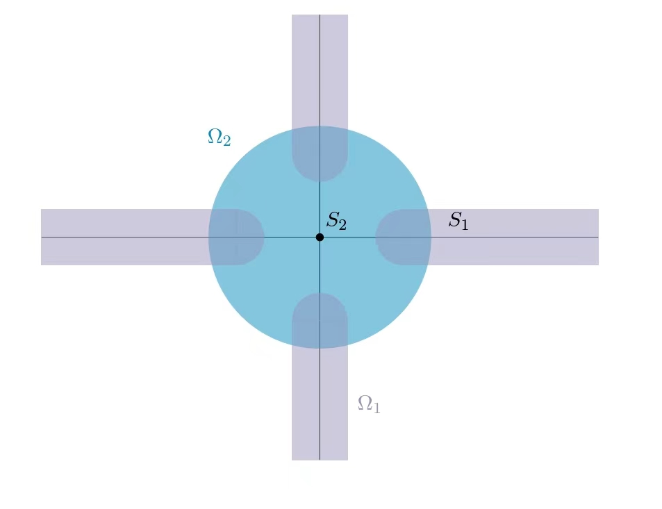
Figure 2: Local picture near $S_{2}$

3.2 Associated non-Morse functions

For $k=1,\cdots,{\mathfrak{k}}$, let $\phi_{k}:S\to[0,\infty]$ be a smooth function such that

1. $\phi_{k}$ has a compact support inside $\Omega_{k}$,

2. $\phi_{k}^{-1}(+\infty)=\Omega^{\prime\prime}_{k}$.

For $k=1,\cdots,{\mathfrak{k}}$, let $\phi_{k,R}$ be a smooth family of functions in $C^{\infty}(S)$, parameterized by $R\in[0,+\infty)$. Here, $\phi_{k,R}$ should be thought of as a smoothed version of the function $\min\{\phi_{k},R\}$, such that:

1. $\phi_{k,R=0}\equiv 0.$

2. $\forall R\geq 0$, $\phi_{k,R}$ has a compact support inside $\Omega_{k}$.

3. When $R$ is large enough $\phi_{k,R}|_{\Omega_{k}^{\prime\prime}}=R$, $\phi_{k,R}|_{\Omega_{k}^{\prime}}\leq\phi_{k}|_{\Omega_{k}^{\prime}}$ and $\phi_{k,R}|_{\Omega_{k}-\Omega_{k}^{\prime}}=\phi_{k}$.

4. $\exists C>0$, $\forall R\geq 0$, $|d^{S}\phi_{k,R}|\leq CR$ and $\left|\frac{\partial\phi_{k,R}}{\partial R}\right|\leq C$.

Fix $r_{1},r_{2}\in(0,1),r_{1}<r_{2}$ to be determined later (See Definition 11.1). Let $q_{A}$ be a smooth family of smooth function on $[0,\infty)$ parametrized by $A\in[0,\infty)$, s.t. (see also the picture below)

1. $q_{A=0}\equiv 0.$

2. $q_{A}|_{[0,r_{1}]}\equiv-A(r_{2}-r_{1})^{2}/2$, and $q_{A}|_{(r_{2},\infty)}\equiv 0.$

3. $q_{A}(\frac{r_{1}+r_{2}}{2})=-\frac{(r_{1}-r_{2})^{2}}{4}.$

4. Near but not at $r_{1}$ and $r_{2}$, $q_{A}$ is quadratic:

   $$q_{A}|_{[r_{1},0.51r_{1}+0.49r_{2}]}(s)=A\varphi\big{(}2e^{A^{2}}(s-r_{1})\big{)}\times(s-r_{1})^{2}/2-A(r_{2}-r_{1})^{2}/2\qquad\text{and}$$

   $$q_{A}|_{[0.49r_{1}+0.51r_{2},r_{2}]}(s)=-A\varphi\big{(}2e^{A^{2}}(r_{2}-s)\big{)}\times(s-r_{2})^{2}/2,$$

   where $\varphi\in C_{c}^{\infty}([0,\infty))$ is a cut-off function such that $0\leq\varphi\leq 1$, $\varphi_{[0,(r_{2}-r_{1})/8]}\equiv 0,$ $\varphi_{[(r_{2}-r_{1})/4,\infty]}\equiv 1,$ $|\varphi^{\prime}|\leq c_{1}$ and $|\varphi^{\prime\prime}|\leq c_{2}$ for some constants $c_{1}$ and $c_{2}$ depending only on $r_{2}-r_{1}.$

5. $C_{1}A\leq{q_{A}^{\prime}(s)}\leq 2C_{1}A$, $|q_{A}^{\prime\prime}|\leq C_{2}A$ for some universal positive constants $C_{1}$ and $C_{2}$ whenever $s\in[0.51r_{1}+0.49r_{2},0.49r_{1}+0.51r_{2}].$

The existence of $q_{A}$ follows from [47, Lemma 2.3].

Figure 3: The graph of $q_{A}$

By Observation 3.4, we have ${\mathfrak{k}}$ functions $q_{k,A}\in C^{\infty}(\pi^{-1}(\Omega_{k}))$, such that for ${\theta}\in\Omega_{k}$

$$q_{k,A}|_{Z_{\theta}-V_{k,{\theta}}}=0\text{ and }q_{k,A}=q_{A}\left(\sqrt{u_{0}^{2}+\cdots+u_{n}^{2}}\right)\text{ on each component of }V_{k,{\theta}}.$$

For $k=1,\cdots,{\mathfrak{k}}$, let $\psi_{k,R}\in C^{\infty}(\pi^{-1}(\Omega_{k}))$ be such that for each ${\theta}\in\Omega_{k}$, $\psi_{k,R}|_{Z_{\theta}}=q_{k,A}$ for $A=\phi_{k,R}({\theta}).$ Then $\psi_{k,R}$ has a compact support inside $\pi^{-1}(\Omega_{k})\cap V$, and we can extend $\psi_{k,R}$ to a smooth function on $M$.

Assumption 3.5.

To avoid heavy notation and overwhelming the reader with technical details, we will temporarily assume that $S_{k}$ is empty, $k\geq 3.$ That means on each fiber, $f$ has at most two birth-death points.

Throughout this paper, except in section 13, we shall assume that $f$ satisfies the Assumption 3.5.

Definition 3.6 (Associated non-Morse functions).

Let $f_{1,T,R}:=Tf+T\psi_{1,R}$ and $f_{2,T,R,R^{\prime}}=Tf+T\psi_{1,R}+T\psi_{2,R^{\prime}}$. We will call $\{f_{1,T,R},f_{2,T,R,R^{\prime}}\}$ the associated non-Morse functions for the fiberwise generalized Morse function $f$.

Remark 3.7.

In the same way, if $f_{{\theta}}$ admits at most ${\mathfrak{k}}$ birth-death points for ${\theta}\in S$ with ${\mathfrak{k}}>2$, then there will be ${\mathfrak{k}}$ associated non-Morse functions as described in Definition 3.6.

We can also assume that $h^{F},\nabla^{F}$ are standard inside $V$, in the sense that

Condition 3.8.

1. Let $i:\Omega_{1}\to V_{1}$ be the section giving the center of the ball that forms of the bundle $V_{1}\to\Omega_{1}$, where $V_{1}\to\Omega_{1}$ is the bundle described in Observation 3.4. We may assume that $F|_{V_{1}}=\pi^{*}\circ i^{*}F|_{V_{1}}$, $h^{F}|_{V_{1}}$ is the pullback of some Hermitian metric $h^{i^{*}F|_{V_{1}}}$ and $\nabla^{F}|_{V_{1}}$ is the pullback of some compatible unitarily connection $\nabla^{i^{*}F|_{V_{1}}}$.

2. Let $i_{1},i_{2}:\Omega_{2}\to V_{2}$ be the two sections giving the centers of the balls that form the bundle $\pi|_{V_{2}}:V_{2}\to\Omega_{2}$. Let $V_{2,a}$, $a=1,2$ be the two connected components of $V_{2}$, then $\pi_{a}:V_{2,a}\to\Omega_{2}$ is a one-ball bundle. We may assume that $F|_{V_{2}}=\pi_{1}^{*}\circ i_{1}^{*}F|_{V_{2}}\sqcup\pi_{2}^{*}\circ i_{2}^{*}F|_{V_{2}}$, $h^{F}|_{V_{2}}$ is the pullback of some Hermitian metric $h^{i_{1}^{*}F|_{V_{1}}}\oplus h^{i_{2}^{*}F|_{V_{2}}}$ and $\nabla^{F}|_{V_{2}}$ is the pullback of some compatible unitarily connection $\nabla^{i_{1}^{*}F|_{V_{2}}}\oplus\nabla^{i_{2}^{*}F|_{V_{2}}}$.

3. Of course, the Hermitian metrics $h^{i^{*}F|_{V_{1}}}$ and $h^{i_{1}^{*}F|_{V_{1}}}\oplus h^{i_{2}^{*}F|_{V_{2}}}$ should agree on $\Omega_{1}\cap\Omega_{2}$, and the unitarily connections $\nabla^{i^{*}F|_{V_{1}}}$ and $\nabla^{i_{1}^{*}F|_{V_{2}}}\oplus\nabla^{i_{2}^{*}F|_{V_{2}}}$ should also agree on $\Omega_{1}\cap\Omega_{2}$.

3.3 Independence of critical points

Definition 3.9.

Let $f:Z\to\mathbb{R}$ be a (generalized) Morse function on a Riemannian manifold $(Z,g^{TZ})$, and $p$ be a critical point of $f$.

A vector field ${\mathcal{V}}\subset\Gamma(TZ)$ is called a gradient-like vector field, if

1. ${\mathcal{V}}=-\nabla f$ in a small neighborhood of critical points of $f$.

2. Away from critical points of $f$, $g^{TZ}({\mathcal{V}},\nabla f)<0$.

Definition 3.10.

Let $f:Z\to\mathbb{R}$ be a (generalized) Morse function on a Riemannian manifold $(Z,g^{TZ})$, and $p$ be a critical point of $f$.

Let $\varphi^{t}$ be the flow generated by a gradient-like flow ${\mathcal{V}}$, then the unstable manifold of $p$ w.r.t. ${\mathcal{V}}$ is defined as $\mathrm{W}^{\mathrm{u}}_{{\mathcal{V}}}(p):=\{q\in Z:\lim_{t\to-\infty}\phi^{t}(q)=p\}$; the stable manifold of $p$ is defined as $\mathrm{W}^{\mathrm{s}}_{\mathcal{V}}(p):=\{q\in Z:\lim_{t\to\infty}\phi^{t}(q)=p\}$.

For any $c>0$, the unstable level set of $p$ is defined as $\mathrm{W}^{\mathrm{u}}_{{\mathcal{V}},c}(p):=\{q\in Z:\lim_{t\to-\infty}\phi^{t}(q)=p\}\cap\{q\in Z:f(q)=f(p)-c\}$; for any $c>0$, the stable level set of $p$ is defined as $\mathrm{W}^{\mathrm{s}}_{{\mathcal{V}},c}(p):=\{q\in Z:\lim_{t\to\infty}\phi^{t}(q)=p\}\cap\{q\in Z:f(q)=f(p)+c\}$.

We say $(f,{\mathcal{V}})$ (or $(f,g^{TZ})$) satisfied Thom-Smale transversality condition (see also [10, p. 219]), if any pair $(p,q)$ of critical point of $f$, $\mathrm{W}^{\mathrm{s}}_{{\mathcal{V}}}(p)$ and $\mathrm{W}_{{\mathcal{V}}}^{\mathrm{u}}(q)$ (or $\mathrm{W}^{\mathrm{s}}_{-\nabla f}(p)$ and $\mathrm{W}_{-\nabla f}^{\mathrm{u}}(q)$) intersect transversely. We will also abbreviate $\mathrm{W}^{\mathrm{s}/\mathrm{u}}_{{\mathcal{V}}}(p)/\mathrm{W}^{\mathrm{s}/\mathrm{u}}_{{\mathcal{V}},c}(p)$ as $\mathrm{W}^{\mathrm{s}/\mathrm{u}}(p)/\mathrm{W}_{c}^{\mathrm{s}/\mathrm{u}}(p)$ if there is no need to emphasis the vector field.

Definition 3.11 (Independence of critical points).

Let $f:Z\to\mathbb{R}$ be a generalized Morse function. We say two critical points $p$ and $q$ of $f$ are independent (for ${\mathcal{V}}$), if $(\mathrm{W}_{\mathcal{V}}^{\mathrm{u}}(p)\cup\mathrm{W}_{\mathcal{V}}^{\mathrm{s}}(p))\cap(\mathrm{W}_{\mathcal{V}}^{\mathrm{u}}(q)\cup\mathrm{W}_{\mathcal{V}}^{\mathrm{s}}(q))=\emptyset$.

We say a critical point $p$ of $f$ is independent (for ${\mathcal{V}}$) if $p$ is independent of any other critical points of $f.$

This definition is taken from [25, p. 62]. An other way to state it is that $p$ and $q$ are independent iff there is no point flowing from one to the other for $t$ going from $-\infty$ to $+\infty$.

Suppose we have a splitting $TM=T^{H}M\oplus TZ$ and a metric $g^{TS}$ on $TS\to S$. Then we take $g^{TM}$ to be $g^{TZ}\oplus g^{TS}$ w.r.t. the splitting above.

Definition 3.12 (Fiberwise gradient vector fields).

Let $f\in C^{\infty}(M)$ be a fiberwise generalized Morse functions for the fibration $\pi:M\to S,$ and $g^{TM}$ be the Riemannian metric introduced above.

Then the fiberwise gradient vector field is $\nabla^{v}f:=P^{TZ}\nabla f$. Here $P^{TZ}$ is the projection w.r.t. the splitting above, and $\nabla f$ is the gradient of $f$ w.r.t. $g^{TM}.$ One can see that $\nabla^{v}f$ is independent of the choice of $g^{TS}.$

Likewise, we could introduce fiberwise gradient-like vector fields, fiberwise stable/unstable manifolds, fiberwise Thom-Smale transversality conditions, fiberwise independence, etc.

The following lemma would be needed, and is an adaptation of [27, Lemma 4.5.1].

Lemma 3.13.

Let $f:M\to\mathbb{R}$ be a fiberwise (generalized) Morse function w.r.t. the fibration $\pi:M\to S$.

Let $\Sigma^{\prime}$ be equal to $\Sigma^{(1,k)}(f)$ or an connected components of $\Sigma^{(0,k)}(f)$ that is disjoint from $\Sigma^{(1)}(f).$ We assume that, for any $p\in\Sigma^{\prime}$, there are $c=c(p)>0$ and a smooth closed ball $D_{p}^{\mathrm{s}/\mathrm{u}}\subset\{x\in Z_{\pi(p)}:f_{\pi(p)}(x)=f_{\pi(p)}(p)\pm c(p)\}$ depending smoothly on $p\in\Sigma^{\prime}$, such that $\mathrm{W}^{\mathrm{s}/\mathrm{u}}_{-\nabla^{v}f|_{Z_{\pi(p)}},c}(p)\subset D_{p}^{\mathrm{s}/\mathrm{u}}$. Here by ‘closed ball’, we mean a smooth manifold with boundary that is homeomorphic to a bounded closed ball $\{x\in\mathbb{R}^{k^{\prime}}:|x|\leq 1\}$ for some $k^{\prime}.$

Let $U,U^{\prime}$ be any two small enough neighborhood of $\Sigma^{\prime}$, s.t. $\bar{U}\subset U^{\prime}$.

For any $q\in\Sigma^{(j,l)}(f)$ satisfying

$$\pi(p)=\pi(q),\qquad|f_{\pi(p)}(q)-f_{\pi(p)}(p)|>c\qquad\text{and}$$

$$1+{\dim(S)}\leq l,k\leq n+1-{\dim(S)}-j-1=\operatorname{dim}Z-\operatorname{dim}S-j-1,$$

there is a fiberwise gradient-like vector field ${\mathcal{V}}$ for $f$, which fiberwisely equal to the vertical gradient $\nabla^{v}f$ outside $U^{\prime}-\bar{U}$, and for which $p$ is independent of $q$.

An other way of saying this is that for any such $q$, there is a deformation of metric $g^{TZ}$ inside $U^{\prime}-\bar{U}$ such that $p$ is independent of $q$ for $\nabla^{v}f$.

Remark 3.14.

In this lemma, in the case where $\Sigma^{\prime}=\Sigma^{(1,k)}(f)$, by the proof of [27, Lemma 4.5.1] we can see that the existence of a ball containing $\mathrm{W}^{\mathrm{s}/\mathrm{u}}_{-\nabla^{v}f|_{Z_{\pi(p)}},c}(p)$ is in fact automatic.

Proof.

The proof is essentially the same as the proof of [27, Lemma 4.5.1].

By symmetry, we may assume that $f(p)>f(q)$, so we must have $f(p)-c>f(q)$ by assumption.

Fix $c^{\prime}\in(0,c),$ such that $(f(p)-c,f(p)-c^{\prime})$ has no critical value of $f$. Let $V_{c,c^{\prime}}$ be some open subset, s.t.,

$$V_{c,c^{\prime}}\subset U_{c,c^{\prime}}:=\left\{x\in Z_{\pi(p)}:f_{\pi(p)}(x)\in\left(f_{\pi(p)}(p)-c,f_{\pi(p)}(p)-c^{\prime}\right)\right\},$$

$${V}_{c,c^{\prime}}\supset U_{c,c^{\prime}}\cap\mathrm{W}^{\mathrm{u}}(p).$$

Let $L_{c}:=\{x\in Z_{\pi(p)}:f_{\pi(p)}(x)=f_{\pi(p)}(p)-c\}$.

Recall that an isotopy of a smooth manifold $X$ is a family of diffeomorphism $\Phi_{\tau}:X\to X$ parametrized by $\tau\in[0,1]$, s.t. $\Phi_{0}$ is the identity map. Deforming the gradient field to gradient-like vector field inside $V_{c,c^{\prime}}$ (or deforming the metric inside $V_{c,c^{\prime}}$) will result in an isotopy of the level surface $L_{c}$. More explicitly, let ${\mathcal{V}}$ be any gradient-like vector field of $f$, s.t. outside $V_{c,c^{\prime}}$, ${\mathcal{V}}=-\nabla^{v}f.$ Let ${\mathcal{V}}(\tau):=\tau{\mathcal{V}}-(1-\tau)\nabla^{v}f$, and define a vector field inside $\bar{U}_{c,c^{\prime}}$ as follows: $\tilde{{\mathcal{V}}}(\tau):=\frac{-{\mathcal{V}}(\tau)}{g^{TZ}\left({\mathcal{V}}(\tau),\nabla^{v}f\right)}$. Then we can see that $\tilde{{\mathcal{V}}}(\tau)(f)=-1.$ Let $\phi^{t}_{\tau}$ be the gradient flow generated by $\tilde{{\mathcal{V}}}(\tau).$ One can also see easily that $\Phi_{\tau}:=\phi^{c-c^{\prime}}_{\tau}\circ\phi^{c^{\prime}-c}_{0}$ is an isotopy of $L_{c}$ and $\Phi_{\tau}(\mathrm{W}^{\mathrm{u}/\mathrm{s}}_{-\nabla^{v}f,c}(p))=\mathrm{W}^{\mathrm{u}/\mathrm{s}}_{{\mathcal{V}}(\tau),c}(p)$.

To make $p$ independent of $q$, we construct an isotopy of the level surface $L_{c}$ as follows. Assume that we have a point $w(p)$ near or inside the disc $D^{\mathrm{u}}_{p}$ so that $\mathrm{W}^{\mathrm{s}}(q)\cap L_{c}$ doesn’t hit that point. Then by an isotopy of $L_{c}$, we can shrink the ball $D^{\mathrm{u}}_{p}$ into a small neighborhood of $w(p)$ so that $\mathrm{W}^{\mathrm{u}}_{c}(p)$ and $\mathrm{W}^{\mathrm{s}}(q)\cap L_{c}$ don’t meet (also note that $L_{c}$ is a manifold without boundary, and $D^{\mathrm{u}}_{p}$ is a manifolds with boundary, so $L_{c}$ contains the closure of $D^{\mathrm{u}}_{p}$). We can realize this isotopy by either deforming the metric inside $V_{c,c^{\prime}}$ or deforming the gradient inside $V_{c,c^{\prime}}$ to a gradient-like vector field.

Hence, we need a smooth function $w:\Sigma^{\prime}\to M$ so that

1. $w(p)\in L_{c}$ for all $p\in\Sigma^{\prime}$,

2. $w(p)$ lies arbitrarily close to $D_{p}^{\mathrm{u}}$,

3. $w(p)\notin\mathrm{W}^{\mathrm{s}}(q)$.

In fact, any generic choice of a function $w$ satisfying (a) and (b) will also satisfy (c) by transversality. Indeed, the set of points in $L_{c}\cap W^{\mathrm{s}}(q)$ has codimension $l$ in $L_{c}$, and the corank is at least $\dim(S)+1$ so in an ${\dim(S)}$-parameters family $\left(\Sigma^{\prime}\right.$ being a $\dim(S)$ or ${\dim(S)}-1$-manifold) this set will be disjoint from a generic $w(p)$. ∎

4 Model Near Birth-death Points

In this section, we will study the model near birth-death points, specifically focusing on Witten deformation for associated non-Morse functions on $\mathbb{R}^{n+1}$ (and $n$ should be large enough). We will introduce a family of generalized Morse functions $f_{y}:\mathbb{R}^{n+1}\to\mathbb{R}$ parameterized by $y\in(-\delta,\delta)$ for some small $\delta>0$. We will then deform $f_{y}$ using a non-Morse function $q_{A}$ introduced earlier. When $A$ is large, this deformation results in the addition of six new Morse points near the birth-death point. In section 5, we will employ Lemma 3.13 to ensure these points are independent of all other critical points. To apply Lemma 3.13, we will analyze their unstable level sets, ensuring that the unstable level set (Definition 3.10) is contained within a topological ball.

For any $r>0,$ let $D_{r}:=\left\{u\in\mathbb{R}^{n+1}:|u|\leq r\right\}$ and $S_{r}:=\left\{u\in\mathbb{R}^{n+1}:|u|=r\right\}$. Also, for any $r^{\prime\prime}>r^{\prime}>0$,

$$D\left(r^{\prime},r^{\prime\prime}\right)=\left\{u\in\mathbb{R}^{n}:r^{\prime}\leq|u|\leq r^{\prime\prime}\right\}.$$

Let $f_{y}\in C^{\infty}(\mathbb{R}^{n+1})$ be given by

$$f_{y}(u)=u_{0}^{3}-yu_{0}-\|(u_{1},\cdots,u_{i})\|^{2}+\|(u_{i+1},\cdots,u_{n})\|^{2},u=(u_{0},\cdots,u_{n})\in\mathbb{R}^{n+1}$$

for $y\in\mathbb{R}$ being small enough and $i\in\{2,\cdots,n-1\}$ being fixed.

Fix $r_{1},r_{2}\in\mathbb{R}$, s.t. $0<r_{1}<r_{2}<\frac{1}{14}$, and let $\delta\in(0,\frac{r_{1}}{24})$ be small enough. Then there exists $\eta\in C^{\infty}([0,\infty))$ such that

Condition 4.1.

1. $\eta\geq 0$ ,$\eta|_{[0,\frac{r_{1}}{6}]}\equiv 0$ and $\eta|_{[\frac{5r_{2}}{2},\infty)}\equiv 0.$

2. $\eta|_{(r_{1},r_{2})}(s)=\delta s.$

3. $|\eta^{\prime}|<2\delta.$

4. $\eta(s)>0$ if $s\in(\frac{r_{1}}{6},\frac{5r_{2}}{2})$

Let $\tilde{\eta}\in C^{\infty}([0,\infty))$ be given by

Condition 4.2.

1. $0\leq\tilde{\eta}\leq 1$.

2. $\tilde{\eta}|_{[\frac{r_{1}}{2},r_{2}]}\equiv 1$, $\tilde{\eta}|_{[0,\frac{r_{1}}{6}]}\equiv 0$ and $\tilde{\eta}|_{[\frac{5r_{2}}{2},\infty)}\equiv 0.$

3. $|\tilde{\eta}^{\prime}|\leq\frac{2}{r_{1}}{(\leq\frac{1}{12\delta})}.$

Lemma 4.3.

If $|y|<\delta^{2}$, the function $\tilde{f}_{y}$ given by $\tilde{f}_{y}(u)=f_{y}(u)-\eta(|u|)u_{1}+y\tilde{\eta}(|u|)u_{0}$ has the same critical point as $f_{y}.$

Proof.

We abbreviate $f_{y}$ and $\tilde{f}_{y}$ as $f$ and $\tilde{f}$ respectively. As $f$ and $\tilde{f}$ coincide outside of $D(\frac{r_{1}}{6},\frac{5r_{2}}{2})$, we have to prove that $\tilde{f}$ has no critical point inside $D(\frac{r_{1}}{6},\frac{5r_{2}}{2})$, that is, the equation $\frac{\partial}{\partial u_{k}}\tilde{f}=0,k=0,1,\cdots n$ has no solution inside $D(\frac{r_{1}}{6},\frac{5r_{2}}{2})$.

One computes

$$\frac{\partial}{\partial u_{0}}\tilde{f}=3u_{0}^{2}-y-\eta^{\prime}(|u|)\frac{u_{1}u_{0}}{|u|}+y\tilde{\eta}(|u|)+y\tilde{\eta}^{\prime}(|u|)\frac{u_{0}^{2}}{|u|},$$ (4.1)

$$\frac{\partial}{\partial u_{1}}\tilde{f}=-2u_{1}-\eta(|u|)-\eta^{\prime}(|u|)\frac{u_{1}^{2}}{|u|}+y\tilde{\eta}^{\prime}(|u|)\frac{u_{0}u_{1}}{|u|},$$ (4.2)

$$\frac{\partial}{\partial u_{j}}\tilde{f}=-2u_{j}-\eta^{\prime}(|u|)\frac{u_{1}u_{j}}{|u|}+y\tilde{\eta}^{\prime}(|u|)\frac{u_{0}u_{j}}{|u|},\qquad j\in\{2,\cdots,i\},$$ (4.3)

$$\frac{\partial}{\partial u_{k}}\tilde{f}=2u_{k}-\eta^{\prime}(|u|)\frac{u_{k}u_{1}}{|u|}+y\tilde{\eta}^{\prime}(|u|)\frac{u_{0}u_{k}}{|u|},\qquad k\in\{i+1,\cdots,n\}.$$ (4.4)

Assume that $u$ is a critical point of $\tilde{f}$ with $u\in D(\frac{r_{1}}{6},\frac{5r_{2}}{2})$.

• If $u_{1}=0$, then by (4.2), $\frac{\partial}{\partial u_{1}}\tilde{f}=-\eta(|u|)\neq 0.$ Hence $u_{1}\neq 0$.

• By item (3) in Condition 4.1, item (3) in Condition 4.2, (4.3), (4.4), and the fact that $\frac{|u_{1}|}{|u|}\leq 1$, $\frac{\partial}{\partial u_{\ell}}\tilde{f}=0$ implies that $u_{\ell}=0$ for $\ell\in\{2,\cdots,n\}$ if $\delta$ is small enough.

  One the other hand, we claim that $\frac{\partial}{\partial u_{0}}\tilde{f}=0$ implies that

  $$|u_{0}|\leq 2\delta.$$ (4.5)

  Indeed, if $|u_{0}|>2\delta$, as $|y|<\delta^{2}$, by item (3) in Condition 4.1 and item (3) in Condition 4.2 we get

  $$\ \ \ \ 3u_{0}^{2}-y-\eta^{\prime}(|u|)\frac{u_{1}u_{0}}{|u|}+y\tilde{\eta}(|u|)+y\tilde{\eta}^{\prime}(|u|)\frac{u_{0}^{2}}{|u|}\geq 3u_{0}^{2}-\delta^{2}-4\delta|u_{0}|$$

  $${>6\delta|u_{0}|-\delta^{2}-4\delta|u_{0}|>3\delta^{2}>0.}$$

  Recall that $\delta<\frac{r_{1}}{24}$, so (4.5) gives $|u_{0}|\leq\frac{r_{1}}{12}$. Since moreover $|u|^{2}=u_{0}^{2}+u_{1}^{2}\geq\frac{r_{1}^{2}}{36}$, we have $u_{1}^{2}\geq\frac{r_{1}^{2}}{48}\geq 3u_{0}^{2}$. Hence,

  $$|u_{1}|\geq{\frac{\sqrt{3}}{2}|u|}>\frac{|u|}{2}.$$ (4.6)

  Now, as $|y|<\delta^{2}$, by item (1) and (3) in Condition 4.1, item (3) in Condition 4.2 and (4.6), we have $|\eta(|u|)|\leq 4\delta|u_{1}|$ , $|\eta^{\prime}(|u|)\frac{u_{1}^{2}}{|u|}|\leq 2\delta|u_{1}|$ and $|y\tilde{\eta}^{\prime}(|u|)\frac{u_{0}u_{1}}{|u|}|\leq\delta|u_{1}|/12\leq 2\delta|u_{1}|$. Thus by (4.2),

  $$\left|\frac{\partial}{\partial u_{1}}\tilde{f}\right|\geq(2-8\delta)|u_{1}|\geq(1-4\delta)|u|.$$

  Since $\delta<r_{1}/24<1/4$, this is a contradiction.

As a conclusion, we have proved that $\tilde{f}$ has no critical point inside $D(\frac{r_{1}}{6},\frac{5r_{2}}{2}).$ ∎

Remark 4.4.

Let $\varrho\in[0,1]$. Then one can see that $f_{y}(u)-\varrho\big{(}\eta(|u|)u_{1}+y\tilde{\eta}(|u|)u_{0}\big{)}$ still has the same critical points as $f_{y}$.

Let $q_{A}\in C^{\infty}[0,\infty)$ be the function defined in section 3.2.

Lemma 4.5.

Assume that $|y|<\delta^{2}.$ Let $f_{A,y}\in C^{\infty}(\mathbb{R}^{n+1})$ be given by $f_{A,y}(u)=\tilde{f}_{y}(u)+q_{A}(|u|)=f_{y}(u)-\eta(|u|)u_{1}{+y\tilde{\eta}(|u|)u_{0}}+q_{A}(|u|)$. When $A$ is large enough, $f_{A,0}$ has $7$ critical points. One of them is the original birth-death point $0$ with index $i$, three of them are Morse points near $S_{r_{1}}$, with index $0,i,i-1$ respectively, and three of them are Morse points near $S_{r_{2}}$, with Morse index $1,i+1,i$ respectively. Similarly, $f_{A,y}$ for $y>0$ has $8$ critical points and $f_{A,y}$ for $y<0$ has $6$ critical points.

Proof.

Note that on $D_{r_{1}}$ and outside of $D_{r_{2}}$, $f_{A,y}(u)=\tilde{f}_{y}(u)+\mathrm{Cst}$, so by Lemma 4.3, it has only 0 has a critical point on these regions. Moreover, by our constructions, $f_{A,y}|_{D(r_{1},r_{2})}$ is independent of $y$, so to prove Lemma 4.5, we only have to show that $f_{A,0}|_{D(r_{1},r_{2})}$ has six critical points with the specified Morse indices.

By point (3) in the construction of $q_{A}$ in section 3.2, if $A$ is large enough, $|\nabla f_{A,0}|^{2}\neq 0$ for $|u|\in[0.51r_{1}+0.49r_{2},0.49r_{1}+0.51r_{2}]$.

By Lemma 4.3, there exists $c>0$, s.t. $|\nabla\tilde{f}_{y}|^{2}|_{D(r_{1},r_{2})}\geq c$. One can check by a direct computation that when $|u|\in[r_{2}-e^{-A^{2}}(r_{2}-r_{1})/2,r_{2}]$, $|\nabla(q_{A}(|u|)|\to 0$ uniformly as $A\to\infty.$ Hence $|\nabla f_{A,0}|^{2}\neq 0$ if $|u|\in[r_{2}-e^{-A^{2}}(r_{2}-r_{1})/2,r_{2}]$ and $A$ is large.

On $D(0.49r_{1}+0.51r_{2},r_{2}-e^{-A^{2}}{(r_{2}-r_{1})}/2)$, we have,

$$f_{A,0}=u_{0}^{3}-(u_{1}^{2}+\dots+u_{i}^{2})+(u_{i+1}^{2}+\dots+u_{n}^{2})-\delta|u|u_{1}-\frac{A}{2}(|u|-r_{2})^{2},$$ (4.7)

so we compute

$$\frac{\partial}{\partial u_{0}}{f}_{A,0}=3u_{0}^{2}-\frac{\delta u_{1}u_{0}}{|u|}{+\frac{A(r_{2}-|u|)u_{0}}{|u|}},$$ (4.8)

$$\frac{\partial}{\partial u_{1}}{f}_{A,0}=-2u_{1}-\delta|u|-\frac{\delta u_{1}^{2}}{|u|}{+\frac{A(r_{2}-|u|)u_{1}}{|u|}},$$ (4.9)

$$\frac{\partial}{\partial u_{j}}{f}_{A,0}=-2u_{j}-\frac{\delta u_{1}u_{j}}{|u|}{+\frac{A(r_{2}-|u|)u_{j}}{|u|}},\qquad j\in\{2,\cdots,i\},$$ (4.10)

$$\frac{\partial}{\partial u_{k}}{f}_{A,0}=2u_{k}-\frac{\delta u_{k}u_{1}}{|u|}{+\frac{A(r_{2}-|u|)u_{k}}{|u|}},\qquad k\in\{i+1,\cdots,n\}.$$ (4.11)

Assume that $u$ is a critical point of $f_{A,0}$ with $u\in D(0.49r_{1}+0.51r_{2},r_{2}-e^{-A^{2}}{(r_{2}-r_{1})}/2)$.

If $u_{1}=0$, then by (4.9), $\frac{\partial}{\partial u_{1}}f_{A,0}=-\delta|u|\neq 0.$ Hence $u_{1}\neq 0$. By (4.11) and the fact that $\frac{|u_{1}|}{|u|}\leq 1$, the condition $\frac{\partial}{\partial u_{k}}f_{A,0}=0$ implies $u_{k}=0$ for $k\in\{i+1,\cdots,n\}.$ Furthermore, by (4.10), if $j\in\{2,\cdots,i\}$, the condition $\frac{\partial}{\partial u_{j}}f_{A,0}=0$ implies $u_{j}=0$ or $-2-\frac{\delta u_{1}}{|u|}+\frac{A(r_{2}-|u|)}{|u|}=0.$ However, if $-2-\frac{\delta u_{1}}{|u|}+\frac{A(|u|-r_{1})}{|u|}=0$, then

$$\frac{\partial}{\partial u_{1}}f_{A,0}=-\delta|u|\neq 0.$$

To sum up, we have proved so far that $u_{1}\neq 0$ and $u_{\ell}=0$ for $2\leq\ell\leq n$. Conversely, if these are satisfied we automatically have $\frac{\partial}{\partial u_{\ell}}f_{A,0}=0$ for $2\leq\ell\leq n$.

We now need to solve the equations $\frac{\partial}{\partial u_{0}}f_{A,0}=0$ and $\frac{\partial}{\partial u_{1}}f_{A,0}=0$ at a point $(u_{0},u_{1},0\dots,0)$, with $u_{1}\neq 0$.

1. If $u_{0}=0$, we automatically have $\frac{\partial}{\partial u_{0}}f_{A,0}=0$.

   Noting that $u_{1}=\pm|u|$ in that case, we can solve $\frac{\partial}{\partial u_{1}}f_{A,0}=0$ and get two solutions:

   $$v_{1,+}(A)=\left(0,\frac{Ar_{2}}{A+2+2\delta},0,\ldots,0\right)$$

   and

   $$v_{2,+}(A)=\left(0,\frac{-Ar_{2}}{A+2-2\delta},0,\ldots,0\right).$$

   For $a=1,2$, we will then abbreviate $v_{a,+}(A)$ as $v_{a,+}$ if it will not cause any confusion.

   One can check directly that:

   $$\mathrm{Hess}(f_{A,0})(v_{1,+})=\mathrm{diag}(2+\delta,-A-2-2\delta,\delta,\ldots,\delta,4+\delta,\ldots,4+\delta).$$

   and

   $$\mathrm{Hess}(f_{A,0})(v_{2,+})=\mathrm{diag}(2-\delta,-A-2+2\delta,-\delta,\ldots,-\delta,4-\delta,\ldots,4-\delta).$$

   Hence, $v_{1,+}$ and $v_{2,+}$ have Morse indices $1$ and $i$, respectively.

2. Now assume $u_{0}\neq 0$. We change the coordinate $(u_{0},u_{1},u_{2},\cdots,u_{n})\to(\gamma,\phi,u_{2},\cdots,u_{n})$ by $u_{0}=\gamma\cos(\phi),u_{1}=\gamma\sin(\phi),u_{2}=u_{2},\cdots,u_{n}=u_{n}.$

   Then for $0.49r_{1}+0.51r_{2}\leq\gamma\leq r_{2}-e^{-A^{2}}{(r_{2}-r_{1})}/2$, by (4.7) we have

   $$f_{A,0}(\gamma,\phi,0,\dots,0)=\gamma^{3}\cos^{3}(\phi)-\gamma^{2}\sin^{2}(\phi)-\delta\gamma^{2}\sin(\phi)-\frac{A}{2}(\gamma-r_{2})^{2},$$

   so we get at a point $(\gamma,\phi,0,\dots,0)$:

   $$F_{1}(\gamma,\phi):=\frac{\partial}{\partial\gamma}{f}_{A,0}=3\gamma^{2}\cos^{3}(\phi)-2\gamma\sin^{2}(\phi)-{2\gamma}\delta\sin(\phi)+{A(r_{2}-\gamma)},$$ (4.12)

   $$F_{2}(\gamma,\phi):=\frac{\partial}{\partial\phi}{f}_{A,0}=-3\gamma^{3}\cos^{2}(\phi)\sin(\phi)-2\gamma^{2}\sin(\phi)\cos(\phi)-\delta\gamma^{{2}}\cos(\phi).$$ (4.13)

   Thus, remembering that $\gamma\cos(\phi)\neq 0$, $\frac{\partial}{\partial\phi}{f}_{A,0}=0$ is equivalent to

   $$3\gamma\sin(\phi)\cos(\phi)+2\sin(\phi)+\delta=0.$$ (4.14)

   We claim that for each fixed $\gamma\in(r_{1},r_{2})$, (4.14) has exactly two solutions , $\phi_{\gamma,\delta,1}$ and $\phi_{\gamma,\delta,2}$, in the interval $(0,2\pi]$, such that

   $$\phi_{\gamma,\delta,1}\in\Big{(}\pi,\frac{3\pi}{2}\Big{)}\text{ and }\phi_{\gamma,\delta,2}\in\Big{(}\frac{3\pi}{2},2\pi\Big{)}.$$ (4.15)

   Indeed, let $g(\phi)=3\gamma\sin(\phi)\cos(\phi)+2\sin(\phi)+\delta$, then $g^{\prime}(\phi)=6\gamma X^{2}+2X-3\gamma$ with $X=\cos(\phi)$. Using the fact that $0<\gamma<r_{2}<\frac{1}{14}$, we find that this polynomial in $X$ has one root $<-1$ and one root $x_{0}\in(0,1)$. We can thus study the variations of $g(\phi)$, according to the sign of $\cos(\phi)-x_{0}$, and we get the claim by noting that $g(\pi)=g(2\pi)=\delta>0$ and $g(3\pi/2)=-2+\delta<0$.

   However, note that

   $$\frac{\partial}{\partial\gamma}f_{A,0}-\frac{\sin(\phi)}{\gamma\cos(\phi)}\frac{\partial}{\partial\phi}f_{A,0}=3\gamma^{2}\cos(\phi){-\gamma\delta\sin(\phi)}+A(r_{2}-\gamma),$$

   which is $>0$ if $\phi\in(\frac{3\pi}{2},2\pi)$. Thus, at a critical point, $\phi=\phi_{\gamma,\delta,1}$.

   Let us give a more precise estimate for $\phi_{\gamma,\delta,1}$ as in (4.15). As $0<\gamma<r_{2}<1/3$, we know that for any $\phi$, $2+3\gamma\cos(\phi)\geq 2-3\gamma>1$, so using (4.14), we get $\sin(\phi_{\gamma,\delta,1})\in\left(-\delta,0\right)\subset\left(-\frac{1}{24},0\right)$. Hence,

   $$\phi_{\gamma,\delta,1}\in(\pi,\varphi_{0}),$$ (4.16)

   where $\varphi_{0}$ is the unique solution of $\sin(\varphi_{0})=-\frac{1}{24}$ in $(\pi,\frac{3\pi}{2})$.

   Let $F:=(F_{1},F_{2})$. Then by the discussion above, finding critical points for $f_{A,0}$ on $D\left(0.49r_{1}+0.51r_{2},r_{2}-\frac{e^{-A^{2}}(r_{2}-r_{1})}{2}\right)$ with $u_{0}\neq 0$ is equivalent to finding zero points of $F:[0.49r_{1}+0.51r_{2},r_{2}-\frac{e^{-A^{2}}(r_{2}-r_{1})}{2}]\times[\pi,\varphi_{0}]\to\mathbb{R}^{2}$.

   First, note that $24^{2}-1>23^{2}$, we have for $\phi\in(\pi,\varphi_{0})$:

   $$\sin(\phi)\in\left(-\frac{1}{24},0\right)\mbox{ and }\cos(\phi)\in\left(-1,-\frac{23}{24}\right).$$ (4.17)

   On the one hand, we have $3\gamma^{2}\cos(\phi_{\gamma,\delta,1})\geq-3\gamma^{2}>-0.3\gamma$, and so

   $$3\gamma^{2}\cos(\phi_{\gamma,\delta,1})+A(r_{2}-\gamma){-\gamma\delta\sin(\phi_{\gamma,\delta,1})}\bigg{|}_{\gamma=\frac{Ar_{2}}{A+0.3}}>{-\gamma\delta\sin(\phi_{\gamma,\delta,1})}>0,$$

   and on the other hand, by (4.17), since

   $$\ \ \ \ \limsup_{A\to\infty}3\gamma^{2}\cos(\phi_{\gamma,\delta,1})+A(r_{2}-\gamma){-\gamma\delta\sin(\phi_{\gamma,\delta,1})}\bigg{|}_{\gamma=r_{2}-e^{-A^{2}}(r_{2}-r_{1})/2}$$

   $$=\limsup_{A\to\infty}3r_{2}^{2}\cos(\phi_{\gamma,\delta,1}){-r_{2}\delta\sin(\phi_{\gamma,\delta,1})}\bigg{|}_{\gamma=r_{2}-e^{-A^{2}}(r_{2}-r_{1})/2}{<0},$$

   we have $3\gamma^{2}\cos(\phi_{\gamma,\delta,1})+A(r_{2}-\gamma){-\gamma\delta\sin(\phi_{\gamma,\delta,1})}\bigg{|}_{\gamma=r_{2}-e^{-A^{2}}(r_{2}-r_{1})/2}<0$ if $A$ is large.

   As a result, a solution of $F=0$ on $\Big{[}0.49r_{1}+0.51r_{2},r_{2}-\frac{e^{-A^{2}}(r_{2}-r_{1})}{2}\Big{]}\times[\pi,\varphi_{0}]$ exists.

   To show uniqueness, we compute the Jacobian matrix of $F$ on $\Big{[}0.49r_{1}+0.51r_{2},r_{2}-\frac{e^{-A^{2}}(r_{2}-r_{1})}{2}\Big{]}\times[\pi,\varphi_{0}]$. Using (4.17) and the fact that $\gamma\in(0,r_{2})\subset(0,1/14),\delta\in(0,{\gamma}/{24})$ we find that if $A$ is large,

   $$\frac{\partial}{\partial\gamma}F_{1} =-A-6\gamma\cos^{3}(\phi)-2\sin^{2}(\phi)-2\delta\sin(\phi)<-\frac{A}{2},$$

   $$\frac{\partial}{\partial\phi}F_{2} =-3\gamma^{3}\cos(\phi)+9\gamma^{3}\cos(\phi)\sin^{2}(\phi)-2\gamma^{2}\cos(2\phi)+\delta\gamma^{2}\sin(\phi)$$

   $$<-2\gamma^{2}\cos(2\phi)+13\gamma^{3}<\gamma^{2}(-1+13\gamma)<-\frac{1}{14^{3}}.$$

   Also, we have:

   $$\left|\frac{\partial}{\partial\phi}F_{1}\right|=\left|\frac{\partial}{\partial\gamma}F_{2}\right|=\Big{|}-9\gamma^{2}\cos^{2}(\phi)\sin(\phi)-4\gamma\sin(\phi)\cos(\phi)-2\delta\gamma\cos(\phi)\Big{|}\leq 9\gamma^{2}+4\gamma+2\delta\gamma.$$

   Hence, the Jacobian matrix of $F$ is negative definite on

   $$\Big{[}0.49r_{1}+0.51r_{2},r_{2}-\frac{e^{-A^{2}}(r_{2}-r_{1})}{2}\Big{]}\times[\pi,\varphi_{0}]$$

   if $A$ is large.

   Thus, by the global version of the inverse function theorem, $F=0$ has a unique solution, say $(\gamma_{A,\delta},\phi_{A,\delta})$, on $[0.49r_{1}+0.51r_{2},r_{2}-\frac{e^{-A^{2}}(r_{2}-r_{1})}{2}]\times[\pi,\varphi_{0}]$. Moreover,

   $$\gamma_{A,\delta}\in\left(\frac{Ar_{2}}{A+0.3},r_{2}-e^{-A^{2}}\frac{(r_{2}-r_{1})}{2}\right)\text{ and }\phi_{A,\delta}=\phi_{\gamma_{A,\delta},\delta,1}\in(\pi,\phi_{0}).$$ (4.18)

   Let $w_{+}:=(\gamma_{A,\delta}\cos(\phi_{A,\delta}),\gamma_{A,\delta}\sin(\phi_{A,\delta}),0,\cdots,0)$. One computes that $\frac{\partial^{2}}{\partial u_{k}\partial u_{l}}f_{A,0}(w_{+})=0$ if $2\leq k<l\leq n$. For $2\leq j\leq i$:

   $$\frac{\partial^{2}}{\partial u_{j}^{2}}f_{A,0}(w_{+})=-2-3\gamma_{A,\delta}\cos^{3}(\phi_{A,\delta})+2\sin^{2}(\phi_{A,\delta})+\delta\sin(\phi_{A,\delta})<-1,$$

   and for $i+1\leq k\leq n$:

   $$\frac{\partial^{2}}{\partial u_{k}^{2}}f_{A,0}(w_{+})=2-3\gamma_{A,\delta}\cos^{3}(\phi_{A,\delta})+2\sin^{2}(\phi_{A,\delta})+\delta\sin(\phi_{A,\delta})>1.$$

   Therefore, together with the negativity of the Jacobian matrix of $F$, we can see that $w_{+}$ has Morse index $i+1$.

Similarly, on $D(r_{1},0.51r_{1}+0.49r_{2})$ we can find another three critical points $v_{1,-},v_{2,-}$ and $w_{-}$, which are near $S_{r_{1}}$ and have Morse index $0,i-1,i$ respectively. This complete the proof. ∎

Remark 4.6.

Assuming that the conditions of Lemma 4.5 holds, we can see from its proof that there exist $(A,y)$-independent positive constants $c=c(r_{1},r_{2},\delta),c^{\prime}=c^{\prime}(r_{1},r_{2},\delta)$ and $C=C(r_{1},r_{2},\delta)$, such that if $A$ is large, any two distinct critical points $p,q\in\{v_{1,+},v_{2,+},w_{+}\}$ satisfy $|p-q|\geq c$, $|f_{A,y}(p)-f_{A,y}(q)|\geq c^{\prime}$ and $|f_{A,y}(p)|\leq C.$ Moreover, limits $\lim_{A\to\infty}v_{1,+}(A)$, $\lim_{A\to\infty}v_{2,+}(A)$ and $\lim_{A\to\infty}w_{+}(A)$ exist.

Next we would like to study the unstable/stable level sets of $w_{\pm}$ and $v_{2,\pm}$.

Let $\mathrm{W}^{\mathrm{s}/\mathrm{u}}_{A}(p)$ and $\mathrm{W}^{\mathrm{s}/\mathrm{u}}_{A,c}(p)$ denotes the stable/unstable manifolds and stable/unstable level sets of a critical point $p$ of $f_{A,y}$ w.r.t. the vector field $-\nabla f_{A,y}.$ We will abbreviate $\mathrm{W}^{\mathrm{s}/\mathrm{u}}_{A}(p)$ and $\mathrm{W}^{\mathrm{s}/\mathrm{u}}_{A,c}(p)$ as $\mathrm{W}^{\mathrm{s}/\mathrm{u}}(p)$ and $\mathrm{W}^{\mathrm{s}/\mathrm{u}}_{c}(p)$ sometimes. By the construction of $f_{A,y}$, it’s easy to see that

Lemma 4.7.

Assume that $|y|\leq\delta^{2}.$ Let $\rho:=|u|,$ and $\frac{\partial}{\partial\rho}:=\sum_{l=0}^{n}\frac{u_{l}}{\rho}\frac{\partial}{\partial u_{l}}.$ For any $\varepsilon>0$, there is $C_{0}>3$, independent from $(A,\delta,y)$, s.t

$$\frac{\partial}{\partial\rho}f_{A,0}>{\varepsilon}\text{ if }u\in D\left(\frac{Ar_{1}}{A-C_{0}},\frac{Ar_{2}}{A+C_{0}}\right).$$ (4.19)

Moreover, there exists $(A,y,\delta)$-independent constant $c_{0}>0$, s.t. for any $c>c_{0}$,

$$\mathrm{W}^{\mathrm{s}/\mathrm{u}}_{A,c}(w_{+})\cap{D\left(\frac{Ar_{2}}{A+C_{0}},r_{2}\right)=\emptyset\mbox{ and }\mathrm{W}^{\mathrm{s}/\mathrm{u}}_{A,c}(v_{a,+})\cap D\left(\frac{Ar_{2}}{A+C_{0}},r_{2}\right)}=\emptyset,a=1,2,$$ (4.20)

if $A$ is large enough.

Proof.

We prove the case for $y=0$, the general cases are similar. If $\rho>0$, we compute

$$\frac{\partial}{\partial\rho}f_{A,0}=\frac{1}{\rho}\left(3u_{0}^{3}-2\sum_{j=1}^{i}u_{j}^{2}+2\sum_{k={i+1}}^{n}u_{k}^{2}\right)-\eta^{\prime}(\rho)u_{1}-\eta(\rho)\frac{u_{1}}{\rho}+q_{A}^{\prime}(\rho)$$

$$\geq q_{A}^{\prime}(\rho)-C^{\prime}_{0}\rho$$

for some $(A,{\delta,y})$-independent constant $C^{\prime}_{0}>3.$

Hence, by the construction of $q_{A}$ in section 3.2, we can see that when $A$ is large, if $C_{0}>\frac{\varepsilon+C^{\prime}_{0}}{r_{1}}$, then (4.19) holds.

A straightforward computation shows that there exists a $A$-independent constant $C_{2}>0$, s.t.

$$\sup_{u,u^{\prime}\in D(\frac{Ar_{2}}{A+C_{0}},r_{2})}\left|f_{A,0}(u)-f_{A,0}(u^{\prime})\right|\leq C_{2}r_{2}^{2}.$$ (4.21)

Choose $c_{0}=2C_{2}r_{2}^{2}$, note that $|w_{+}|,|v_{2,+}|\in\Big{(}\frac{Ar_{2}}{A+3},r_{2}\Big{)}$ when $A$ is large enough, so (4.21) implies (4.20). ∎

Remark 4.8.

For $p=w_{+}$ or $v_{a,+},a=1,2$, we define $\widetilde{\mathrm{W}}^{\mathrm{s}/\mathrm{u}}_{A,c}(p):=\mathrm{W}^{\mathrm{s}/\mathrm{u}}_{A,c}(p)\cap\{u:|u|>r_{2}\}$ and ${\widehat{\mathrm{W}}}^{\mathrm{s}/\mathrm{u}}_{A,c}(p):=\mathrm{W}^{\mathrm{s}/\mathrm{u}}_{A,c}(p)\cap\{u:|u|<r_{2}\}$. Then by (4.20), $\widetilde{\mathrm{W}}^{\mathrm{s}/\mathrm{u}}_{A,c}(p)$ and ${\widehat{\mathrm{W}}}^{\mathrm{s}/\mathrm{u}}_{A,c}(p)$ are separated by $D(\frac{Ar_{2}}{A+C_{0}},r_{2})$. In section 5 (see the paragraph below (5.11)), we will show that ensuring the independence of the new critical points described in Lemma 4.5 only involves handling $\widetilde{\mathrm{W}}^{\mathrm{s}/\mathrm{u}}_{A,c}(p)$.

We will also abbreviate $\widetilde{\mathrm{W}}^{\mathrm{s}/\mathrm{u}}_{A,c}(p)$ as $\widetilde{\mathrm{W}}^{\mathrm{s}/\mathrm{u}}_{c}(p)$ sometimes. Because of the above remark, our next lemma will focus on studying $\widetilde{\mathrm{W}}^{\mathrm{s}/\mathrm{u}}_{A,c}(p)$.

Lemma 4.9.

Assume that $|y|\leq\delta^{2}.$ There exists $(A,y,\delta)$-independent constant $c_{0}>0$, s.t. for any $c>c_{0}$, there exist smooth closed balls $D^{\mathrm{s}/\mathrm{u}}_{c}(p)\subset\{u:f_{A,y}(u)=f(p)\pm c\}\cap\{u:|u|>r_{2}\}$ s.t. $\widetilde{\mathrm{W}}^{\mathrm{s}/\mathrm{u}}_{A,c}(p)\subset D^{\mathrm{s}/\mathrm{u}}_{c}(p)$ for $p=w_{+}$ or $v_{a,+}$, $a=1,2$.

Moreover, if we choose $c=c_{A,y,\delta}>c_{0}$ such that $f_{A,y}(p)\pm c$ is independent of $A$, $y$ and $\delta$, then the set $\{u:f_{A,y}(u)=f(p)\pm c\}\cap\{u:|u|>r_{2}\}$ is independent of $A$, $y$ and $\delta$, and $D^{\mathrm{s}/\mathrm{u}}_{c}(p)$ can be taken independent of $A$, $y$ and $\delta$.

Proof.

We prove the case for $y=0$, the general cases are similar. In this proof, for $u=(u_{0},\dots,u_{n})\in\mathbb{R}^{n+1}$, we will set $u^{-}=(u_{1},\dots,u_{i})$ and $u^{+}=(u_{i+1},\dots,u_{n})$.

Let $\phi^{t}$ be the flow generated by $-\nabla f_{A,0}.$

A straightforward computations shows that

$$\begin{cases}|\nabla f_{A,0}|(u)\leq C|u|^{2}\mbox{ for some $A$-independent $C$ if $|u|\geq\frac{Ar_{2}}{A+3}$;}\\ |\nabla f_{A,0}|^{2}(u)\geq C^{-1}|u|^{2}\mbox{ if $|u|\in(\frac{5r_{2}}{2},+\infty)$};\\ \frac{\partial}{\partial u_{l}}f_{A,0}(u)=-2u_{l}\mbox{ if $1\leq l\leq i$, $|u|\geq\frac{5r_{2}}{2}$};\\ \frac{\partial}{\partial u_{l}}f_{A,0}(u)=2u_{l}\mbox{ if $1\leq l\leq i$, $|u|\geq\frac{5r_{2}}{2}$}.\end{cases}$$ (4.22)

These imply that

$$\widetilde{\mathrm{W}}^{\mathrm{u}}(v_{2,+})\cap S_{3r_{2}}\subset\Big{\{}u\in S_{3r_{2}}:\|u^{+}\|\leq\frac{5r_{2}}{2}\Big{\}}.$$ (4.23)

Indeed, if $u\in S_{3r_{2}}$ satisfies $\|u^{+}\|>5r_{2}/2$, we claim that $\left(\cup_{t<0}\phi^{t}(u)\right)\cap S_{5r_{2}/2}=\emptyset$, so it is impossible that $\lim_{t\to-\infty}\phi^{t}(u)=v_{2,+}$. If this claim is not true, i.e., $\left(\cup_{t<0}\phi^{t}(u)\right)\cap S_{5r_{2}/2}\neq\emptyset$, then there exists $t_{0}{<0}$, s.t. $|\phi^{t}(u)|>5r_{2}/2$ for $t\in{(t_{0},0]}$, but $|\phi^{t_{0}}(u)|=5r_{2}/2$. Let $v=(v_{0},\cdots,v_{n})=\phi^{t_{0}}(u)$. By the fourth statement of (4.22), $v_{i+1}^{2}+\cdots+v_{n}^{2}>u_{i+1}^{2}+\cdots u_{n}^{2}>(5r_{2}/2)^{2},$ which contradicts the fact that $\phi^{t_{0}}(u)\in S_{5r_{2}/2}.$

Similarly,

$$\widetilde{\mathrm{W}}^{\mathrm{s}}(v_{2,+})\cap S_{3r_{2}}\subset\Big{\{}u\in S_{3r_{2}}:\|u^{-}\|\leq\frac{5r_{2}}{2}\Big{\}}.$$

Notice that

$$|f_{A,0}(v_{2,+})|=\left|-|v_{2,+}|^{2}+\delta|v_{2,+}|-\frac{A(2-2\delta)^{2}(r_{2}^{2})}{(A+2-2\delta)^{2}}\right|\leq 3r_{2}^{2}$$ (4.24)

if $A$ is large. So there exists $c^{\prime\prime}_{0}$ large enough, s.t. $f_{A,0}(v_{2,+})-c^{\prime\prime}_{0}<0$ and $f_{A,0}(v_{2,+})+c^{\prime\prime}_{0}>0.$

Let $L_{c}=\{u\in\mathbb{R}^{n}:f_{A,0}(u)=f_{A,0}(v_{2,+})-c\}$. By the first statement of (4.22) (also note that $|v_{2,+}|>\frac{Ar_{2}}{A+3}$), we have $\sup_{u\in D(|v_{2,+}|,3r_{2})}|f(u)-f(v_{2,+})|\leq C(3r_{2})^{3}$. So there exists $(A,y,\delta)$-independent $c^{\prime}_{0}>c^{\prime\prime}_{0}>0$ large enough, s.t. if $c>c^{\prime}_{0}$,

$$L_{c}\cap D(|v_{2,+}|,3r_{2})=\emptyset.$$ (4.25)

Assume from now on that $c>c^{\prime}_{0}$. Let $U_{c}\subset L_{c}$ be the set of points $u=(u_{0},\cdots,u_{n})\in L_{c}\cap D(3r_{2},\infty)$, s.t.

1. $u_{0}>3r_{2}$ or

2. $\|u^{+}\|>\frac{5r_{2}}{2}$.

On $D(3r_{2},\infty)$,

$$f_{A,0}=u_{0}^{3}-\|u^{-}\|^{2}+\|u^{+}\|^{2},$$ (4.26)

so

$$\nabla f_{A,0}=(3u_{0}^{2},-2u_{1},\cdots,-2u_{i},2u_{i+1},\cdots,2u_{n}).$$ (4.27)

We must have

$$\forall u\in U_{c},\;\left(\cup_{t<0}\phi^{t}(u)\right)\cap\left(S_{3r_{2}}\cap\widetilde{\mathrm{W}}^{\mathrm{u}}(v_{2,+})\right)=\emptyset.$$ (4.28)

Otherwise, there exists $u\in U_{c}$, such that $\phi^{t_{0}}(u)\in S_{3r_{2}}\cap\widetilde{\mathrm{W}}^{\mathrm{u}}(v_{2,+})$ for some $t_{0}<0$. By (4.25), there exists $t_{1}\in[t_{0},0]$, s.t. $|\phi^{t}(u)|>3r_{2}$ for $t\in(t_{1},0]$ but $|\phi^{t_{1}}(u)|=3r_{2}.$ If $u_{0}>3r_{2}$, then by (4.27), the $0$-th component of $\phi^{t_{1}}(u)$ is greater than $u_{0}>3r_{2}$, which contradicts with $|\phi^{t_{1}}(u)|=3r_{2}$. If $\|u^{+}\|>5r_{2}/2$, we also get a contradiction using (4.23). Thus, (4.28) holds.

By (4.25) and (4.28), we have

$$\widetilde{\mathrm{W}}^{\mathrm{u}}_{c}(v_{2,+})\subset L_{c}\cap\{u\in\mathbb{R}^{n+1}:u_{0}\leq 3r_{2},\|u^{+}\|\leq\frac{5r_{2}}{2}\}\cap D({3}r_{2},\infty).$$

But by (4.26) and our choice of $c_{0}$ and $c_{0}^{\prime}$, $L_{c}\cap\{u\in\mathbb{R}^{n}:u_{0}\leq 3r_{2},\|u^{+}\|\leq 5r_{2}/2\}\cap D({3}r_{2},\infty)$ is contained in a smooth closed topological ball that is independent of $A.$ Indeed, set $\kappa=c-f_{A,0}(v_{2,+})>0$, then

$$L_{c}\cap\Big{\{}u\in\mathbb{R}^{n+1}:u_{0}\leq 3r_{2},\|u^{+}\|\leq\frac{5r_{2}}{2}\Big{\}}\cap D({3}r_{2},\infty)$$

$$=\Big{\{}u\in\mathbb{R}^{n+1}\>:\>u_{0}^{3}-\|u^{-}\|^{2}+\|u^{+}\|^{2}=-\kappa,\,u_{0}\leq 3r_{2},\,\|u^{+}\|\leq\frac{5r_{2}}{2}\Big{\}}.$$

As a consequence, by (4.24), if we set $K=27r_{2}^{3}+(5r_{2}/2)^{2}+\kappa$, we get that $L_{c}\cap\{u\in\mathbb{R}^{n+1}:u_{0}\leq 3r_{2},\|u^{+}\|\leq 5r_{2}/2\}\cap D({3}r_{2},\infty)$ is included in the image $D^{\mathrm{u}}_{c}(v_{2,+})$ of $B^{\mathbb{R}^{i}}(0,K)\times B^{\mathbb{R}^{n-i}}(0,5r_{2}/2)$ under the map $\psi\colon(s,t)\mapsto\big{(}(\|s\|^{2}-\|t\|^{2}-\kappa)^{1/3},s,t\big{)}$, which is a homeomorphism on its image. Note also that, although $\psi$ is not smooth on $\{(s,t):\|s\|^{2}-\|t\|^{2}=\kappa\}$, the set $D^{\mathrm{u}}_{c}(v_{2,+})$ is still smooth.

Moreover, by (4.24), we can take $c_{0}>c^{\prime}_{0}$ large enough so that $c>c_{0}$ implies $\kappa>(3r_{2})^{3/2}+(3r_{2})^{2}$. In that case, $u=\psi(s,t)$, we have either $|s|>3r_{2}$, in which case $\|u\|>3r_{2}$, or $|s|\leq 3r_{2}$, in which case $\kappa-\|s\|^{2}+\|t\|^{2}>(3r_{2})^{3/2}$ so that again, $\|u\|>3r_{2}$. Hence, if $c>c_{0}$, $D^{\mathrm{u}}_{c}(v_{2,+})\subset D(3r_{2},\infty)$.

Now, if we choose $c=c_{A,y,\delta}$ so that $\kappa$ is independent of $A$, $y$ and $\delta$, then by (4.25) and (4.26), $\{u:f_{A,y}(u)=f(v_{2,+})-c\}\cap\{u:|u|>r_{2}\}=\{u:f_{A,y}(u)=-\kappa\}\cap\{u:|u|>3r_{2}\}$ is independent of $A$, $y$ and $\delta$, as well as the map $\psi$, so $D^{\mathrm{u}}_{c}(v_{2,+})$ can be taken independent of $A$, $y$ and $\delta$.

Let $\tilde{L}_{c}=\{u\in\mathbb{R}^{n+1}:f_{A,0}(u)=f_{A,0}(v_{2,-})+c\}.$ Similarly, we can show that for $c$ large enough,

$$\widetilde{\mathrm{W}}^{\mathrm{s}}_{c}(v_{2,+})\subset\tilde{L}_{c}\cap\Big{\{}u\in\mathbb{R}^{n+1}:u_{0}\geq-3r_{2},\|u^{-}\|\leq\frac{5r_{2}}{2}\Big{\}}\cap D({3}r_{2},\infty).$$

While for the same reason, $\tilde{L}_{c}\cap\{u\in\mathbb{R}^{n+1}:u_{0}\geq-3r_{2},\|u^{-}\|\leq 5r_{2}/2\}\cap D({3}r_{2},\infty)$ is contained in a closed ball, that is independent of $A$, $y$ and $\delta$ if $c$ is large and satisfies that $f_{A,y}(p)+c$ does not depend on $A$, $y$ and $\delta$.

Proceeding in the same way, we also have the same statement for $v_{1,+}$ and $w_{+}.$ ∎

5 Analytic and Combinatorial Torsion Forms

5.1 Double suspension and analytic torsion forms

In this section, we will introduce the concept of double suspension. The purpose of performing double suspension is to ensure that the Morse index of all critical points satisfies the lower and upper bounds specified in Lemma 3.13. Then, by using Lemma 3.13, Lemma 4.7, and Lemma 4.9, we will show that the product metric on the double suspended space can be deformed to ensure that the birth-death point and the six new Morse points described in section 4 are independent of other critical points(except for the birth-death point or the two points that converge to the birth-death point as $t_{1}\to 0$ in Lemma 3.2). Based on this, we will introduce higher combinatorial torsion.

Another reason for considering double suspension is the following: for any gradient flow $\gamma$ on a closed manifold, as $t\to\pm\infty$, $\gamma(t)$ must converge to a critical point. However, on a noncompact manifold, the flow may diverge to infinity. This observation, combined with the upper and lower bounds of the Morse index of critical points, enable us to make certain critical points independent.

Definition 5.1.

Let $f:M\to\mathbb{R}$ be a smooth function. A double suspension of the pair $(M,f)$ is the pair $(\mathcal{M},\mathfrak{f})$, where $\mathcal{M}:=M\times\mathbb{R}^{N}\times\mathbb{R}^{N}$,

$$\mathfrak{f}(p,x_{1},x_{2})=f(p)-|x_{1}|^{2}+|x_{2}|^{2},\forall(p,x_{1},x_{2})\in M\times\mathbb{R}^{N}\times\mathbb{R}^{N}$$

for some large enough even number $N.$

One can see ${{{\pi^{\mathrm{sp}}}}\colon}\mathcal{M}\to S$ is a fibration with fiber $\mathcal{Z}:=Z\times\mathbb{R}^{N}\times\mathbb{R}^{N},$ and $\Sigma(\mathfrak{f})=\Sigma(f)\times\{0\}\times\{0\}.$ Moreover, if $\mathfrak{p}=(p,0,0)\in\Sigma(\mathfrak{f})$, then $\mathrm{ind}_{\mathfrak{f}}(\mathfrak{p})=\mathrm{ind}_{f}(p)+N$. From now on, we fix $N$ sufficiently large so that

Condition 5.2.

the Morse indices of all critical points of $\mathfrak{f}_{\theta},{\theta}\in S$ satisfy the lower and upper bounds specified in Lemma 3.13.

Here $\mathrm{ind}_{f}(p)$ denotes the Morse index of a critical point $p\in\Sigma(f).$

Let $T^{H}\mathcal{M}:=T^{H}M\oplus\{0\}\oplus\{0\}$, $g^{T\mathcal{Z}^{\prime}}:=g^{TZ}\oplus g^{T\mathbb{R}^{N}}\oplus g^{T\mathbb{R}^{N}}$, $({\mathcal{F}},h^{{\mathcal{F}}})$ be the pull back of $(F,h^{F})$ w.r.t. the canonical map $\mathcal{M}\to M$, and $\nabla^{{\mathcal{F}}}=\nabla^{F}+\sum_{i=1}^{2N}du_{i+n}\wedge\frac{\partial}{\partial u_{n+i}}$. Here $g^{T\mathbb{R}^{N}}$ is the standard metric on $\mathbb{R}^{N}$ and we denoted $(x_{1},x_{2})=(u_{n+1},\cdots,u_{n+2N})$.

By the theory of harmonic oscillator and proceeding as in the proof of [8, Proposition 3.28], we can see that we can define, for $T>0$, a differential form

$$\mathcal{T}(T^{H}\mathcal{M},g^{T\mathcal{Z}^{\prime}},e^{-2T\mathfrak{f}}h^{{\mathcal{F}}})$$

associated with the above data, as in Definition 2.9, and that moreover,

$$\mathcal{T}^{+}(T^{H}\mathcal{M},g^{T\mathcal{Z}^{\prime}},e^{-2T\mathfrak{f}}h^{{\mathcal{F}}})=\mathcal{T}^{+}(T^{H}M,g^{TZ},e^{-2Tf}h^{F}).$$

Here $w^{+}$ means positive degree component of a differential form $w.$

Let $g^{T\mathcal{Z}}$ be a perturbation of $g^{T\mathcal{Z}^{\prime}}$, such that outside a compact neighborhood of $M\times\{0\}\times\{0\}\subset\mathcal{M}$, $g^{T\mathcal{Z}}=g^{T\mathcal{Z}^{\prime}}$. Using the standard finite-propagation-speed argument, we can see that

$$\mathcal{T}(T^{H}\mathcal{M},g^{T\mathcal{Z}},e^{-2T\mathfrak{f}}h^{{\mathcal{F}}})$$

is also well-defined.

Let ${\mathbf{H}}^{T}$ be the $L^{2}$-cohomology of $(\Omega^{\bullet}(\mathcal{Z},{\mathcal{F}}|_{\mathcal{Z}}),d^{\mathcal{Z}})$ with respect to the $L^{2}$ metric induced by $g^{T\mathcal{Z}}$ and $e^{-2{T}\mathfrak{f}}h^{{\mathcal{F}}}$ (for the definition of $L^{2}$-cohomology, see [15]). Let ${\mathbf{H}}:={\mathbf{H}}^{T=1}$, then ${\mathbf{H}}\to S$ carries a natural Gauss-Manin-type connection $\nabla^{{\mathbf{H}}}$.

Let ${\mathbf{H}}^{T,\prime}$ be the $L^{2}$-cohomology of $(\Omega^{\bullet}(\mathcal{Z},{\mathcal{F}}|_{\mathcal{Z}}),d^{\mathcal{Z}})$ with respect to the $L^{2}$ metric induced by $g^{T\mathcal{Z}^{\prime}}$ and $e^{-2{T}\mathfrak{f}}h^{{\mathcal{F}}}$. Let ${\mathbf{H}}^{\prime}:={\mathbf{H}}^{T=1,\prime}$. Recall that $H\to S$ is the cohomology bundle associated with $M\to S$ and the flat bundle $F\to M$. Then we have a canonical isomorphism between $H$ and ${\mathbf{H}}^{T,\prime}$ given by the following map of closed form

$$w\mapsto\frac{e^{-2T|x_{1}|^{2}}}{{(2\pi T)}^{\frac{N}{2}}}w\wedge dx_{1},$$ (5.1)

where $w$ is a closed form on $Z$. Here $dx_{1}$ is the $N$-form given as follows: write $x_{1}=(u_{n+1},\cdots,u_{n+N})$, then $dx_{1}:=du_{n+1}\wedge\cdots\wedge du_{n+N}.$

Let

$$\mathcal{J}_{T}:{\mathbf{H}}^{T,\prime}\to{\mathbf{H}}^{\prime}$$ (5.2)

be the isomorphism induced by the following map of closed forms $\frac{e^{-2T|x_{1}|^{2}}}{{(2\pi T)}^{\frac{N}{2}}}w\wedge dx_{1}\mapsto\frac{e^{-2|x_{1}|^{2}}}{{(2\pi)}^{\frac{N}{2}}}w\wedge dx_{1},$ where $w$ is a closed form on $Z$.

There is a canonical isomorphism

$$\mathcal{K}_{T}:{\mathbf{H}}^{T,\prime}\to{\mathbf{H}}^{T}$$ (5.3)

given as follows: suppose there is an element $[w]$ in ${\mathbf{H}}^{T,\prime}$ represented by a smooth closed $L^{2}$-form $w$, then $w$ is clearly $L^{2}$-integrable w.r.t. the measure induced by $e^{-2T\mathfrak{f}}h^{{\mathcal{F}}}$ and $g^{T\mathcal{Z}}$, so we simply map $[w]$ to the element in ${\mathbf{H}}^{T}$ represented by $w$. It is also tautological to check that this map is well defined.

Let $h^{{\mathbf{H}}}_{L^{2},T}$ be the Hodge metric on ${\mathbf{H}}$ induced by $g^{T\mathcal{Z}}$, $e^{-2T\mathfrak{f}}h^{{\mathcal{F}}}$, and $\mathcal{K}_{1}\mathcal{J}_{T}\mathcal{K}_{T}^{-1}$. Let $h^{{\mathbf{H}},\prime}_{L^{2},T}$ be the Hodge metric on ${\mathbf{H}}$ induced by $g^{T\mathcal{Z}^{\prime}}$, $e^{-2T\mathfrak{f}}h^{{\mathcal{F}}}$, and $\mathcal{K}_{1}\mathcal{J}_{T}$.

Let $h^{H}_{L^{2},T}$ be the Hodge metric on $H$ induced by $T^{H}M$, $g^{TZ}$, $e^{-2Tf}h^{F}$. We can easily check that the isomorphism (5.1) together with $\mathcal{K}_{1}\mathcal{J}_{T}$ gives an isometric map from $(H,h^{H}_{L^{2},T})$ to $({\mathbf{H}},h^{{\mathbf{H}}^{\prime}}_{L^{2},T})$. Given a metric $h^{H}$ on $H\to S$, let $h^{{\mathbf{H}}}_{T}$ denote the metric on ${\mathbf{H}}\to S$ induced by isomorphism (5.1) and $\mathcal{K}_{1}\mathcal{J}_{T}.$

Recall that $H_{0}\to S$ is the cohomology bundle associated with $M\to S$ and the trivial bundle ${\underline{\mathbb{C}}}^{m}\to M$. Similarly, given a metric $h^{H_{0}}$ on $H_{0}\to S$, we have the corresponding metric $h^{{\mathbf{H}}_{0}}_{T}$ on ${\mathbf{H}}_{0}$. Here, ${\mathbf{H}}_{0}$ is the associated $L^{2}$-cohomology bundle for the trivial flat bundle ${\underline{\mathbb{C}}}^{m}\to\mathcal{M}$ defined in the same way as ${\mathbf{H}}$.

Similarly to Definition 2.10, we can define ${\overline{\widetilde{\mathcal{T}}}}(T^{H}\mathcal{M},g^{T\mathcal{Z}^{\prime}},e^{-2T\mathfrak{f}}h^{{\mathcal{F}}},h^{{\mathbf{H}}}_{T},h^{{\mathbf{H}}_{0}}_{T})$. More explicitly, the metric $h^{H}$ and $h^{H}_{L^{2}}$ in Definition 2.10 are replaced by $h^{{\mathbf{H}}}_{T}$ and $h^{{\mathbf{H}}^{\prime}}_{L^{2},T}$ respectively, etc. The discussion above implies that

$${\overline{\widetilde{\mathcal{T}}}}(T^{H}\mathcal{M},g^{T\mathcal{Z}^{\prime}},e^{-2T\mathfrak{f}}h^{{\mathcal{F}}},h^{{\mathbf{H}}}_{T},h^{{\mathbf{H}}_{0}}_{T})={\overline{\widetilde{\mathcal{T}}}}(T^{H}M,g^{TZ},\nabla^{F},e^{-2Tf}h^{F},h^{H},h^{H_{0}}).$$

Using the standard finite-propagation-speed argument, we can see that

$${\overline{\widetilde{\mathcal{T}}}}(T^{H}\mathcal{M},g^{T\mathcal{Z}},e^{-2T\mathfrak{f}}h^{{\mathcal{F}}},h^{{\mathbf{H}}}_{T},h^{{\mathbf{H}}_{0}}_{T})$$

is also well-defined as in Definition 2.10 (the metric $h^{H}$ and $h^{H}_{L^{2}}$ in Definition 2.10 are replaced by $h^{{\mathbf{H}}}_{T}$ and $h^{{\mathbf{H}}}_{L^{2},T}$ respectively, etc.). Moreover, proceeding as in [8, Theorem 3.24], in $\Omega^{\bullet}(S)/d^{S}\Omega^{\bullet}(S)$,

$${\overline{\widetilde{\mathcal{T}}}}(T^{H}\mathcal{M},g^{T\mathcal{Z}^{\prime}},e^{-2T\mathfrak{f}}h^{{\mathcal{F}}},h^{{\mathbf{H}}}_{T},h^{{\mathbf{H}}_{0}}_{T})={\overline{\widetilde{\mathcal{T}}}}(T^{H}\mathcal{M},g^{T\mathcal{Z}},e^{-2T\mathfrak{f}}h^{{\mathcal{F}}},h^{{\mathbf{H}}}_{T},h^{{\mathbf{H}}_{0}}_{T}).$$

Lastly, if $\tilde{\mathfrak{f}}$ is another smooth function on $\mathcal{M}$, s.t. $\tilde{\mathfrak{f}}=\mathfrak{f}$ outside some compact subset of $\mathcal{M}$, then proceeding as in [8, Theorem 3.24], in $\Omega^{\bullet}(S)/d^{S}\Omega^{\bullet}(S)$,

$${\overline{\widetilde{\mathcal{T}}}}(T^{H}\mathcal{M},g^{T\mathcal{Z}},e^{-2T\tilde{\mathfrak{f}}}h^{{\mathcal{F}}},h^{{\mathbf{H}}}_{T},h^{{\mathbf{H}}_{0}}_{T})={\overline{\widetilde{\mathcal{T}}}}(T^{H}\mathcal{M},g^{T\mathcal{Z}},e^{-2T\mathfrak{f}}h^{{\mathcal{F}}},h^{{\mathbf{H}}}_{T},h^{{\mathbf{H}}_{0}}_{T}).$$

In summary, together with Proposition 2.11, we have shown that

Theorem 5.3.

If $g^{T\mathcal{Z}}=g^{T\mathcal{Z}^{\prime}}$ and $\tilde{\mathfrak{f}}=\mathfrak{f}$ outside some compact subset of $\mathcal{M}$, then for any $T>0,$ the following identity holds

$${\overline{\widetilde{\mathcal{T}}}}(T^{H}\mathcal{M},g^{T\mathcal{Z}},e^{-2T\tilde{\mathfrak{f}}}h^{{\mathcal{F}}},h^{{\mathbf{H}}}_{T},h^{{\mathbf{H}}_{0}}_{T})={\overline{\widetilde{\mathcal{T}}}}(T^{H}M,g^{TZ},h^{F},h^{H},h^{H_{0}})$$

in $\Omega^{\bullet}(S)/d^{S}\Omega^{\bullet}(S)$,

5.2 Definition of higher combinatorial torsions

5.2.1 Combinatorial complex and its torsion

Let $f:M\to\mathbb{R}$ be a fiberwise generalized Morse function satisfying the conditions described in section 3, and $(\mathcal{M},\mathfrak{f})$ is a double suspension of $(M,f)$ for a large enough even number $N.$

Let ${\mathcal{V}}$ be a tubular neighborhood of $\Sigma^{(1)}(\mathfrak{f})$ in $\mathcal{M}$ that satisfies the same conditions as $V$ did in Lemma 3.2. By slightly perturbing $\mathfrak{f}$ in the $Z$ component within ${\mathcal{V}}$ if needed, we assume $\mathfrak{f}$ provides a stratification of $S$ as described in section 3. We can see that $\Omega=\pi({\mathcal{V}})$ is a small “tubular” neighborhood of $L:=\pi(\Sigma^{(1)}(f))={{{\pi^{\mathrm{sp}}}}}(\Sigma^{(1)}(\mathfrak{f}))$. Let also $\Omega_{0}^{\prime\prime}$, $\Omega_{1}$, $\Omega_{1}^{\prime\prime}$, etc., be open sets that are constructed as described in section 3.2.

Moreover, fiberwisely, we assume that ${\mathcal{V}}_{\theta}:=\pi^{-1}({\theta})\cap{\mathcal{V}}$, ${\theta}\in\pi({\mathcal{V}})$, consists of one or two balls of large radius, say equal to $100$, w.r.t. the metric $g^{T\mathcal{Z}}$, and with centers being birth-death points if ${\theta}\in L.$ For $r\in(0,100)$, let ${\mathcal{V}}(r)\subset{\mathcal{V}}$ denotes a neighborhood of $\Sigma^{(1)}(f)$, such that $\pi({\mathcal{V}}(r))=\pi({\mathcal{V}})$ and ${\mathcal{V}}(r)_{\theta}:=\pi^{-1}({\theta})\cap{\mathcal{V}}(r),{\theta}\in\pi({\mathcal{V}})$, consists of the closed balls ${\mathcal{V}}(r)_{\theta}$ with the same center as ${\mathcal{V}}_{\theta}$ but with radius $r$. For $r^{\prime}<r$, let ${\mathcal{V}}(r,r^{\prime}):={\mathcal{V}}(r^{\prime})-\mathring{{\mathcal{V}}}(r).$

Let $0<r_{1}<r_{2}<1$ be constants appearing in the definition of $q_{A}$ in section 3.2.

If $N$ is large enough, by choosing $\Omega$ small enough, we can choose the metric $g^{T\mathcal{Z}}$ (c.f. [27, Lemma 4.5.1] or Lemma 3.13 and Remark 3.14) such that it satisfies the following condition:

Condition 5.4.

1. Fiberwisely, birth-death points (or critical points of $\mathfrak{f}_{\theta}$ which converge to birth-death points as $t_{1}\to 0$, where $t_{1}$ is the function in Lemma 3.2) are independent of other critical points under $g^{T\mathcal{Z}}$, ${\theta}\in\Omega$.

2. we have $g^{T\mathcal{Z}}=g^{T\mathcal{Z}^{\prime}}$ on $\mathcal{M}-{\mathcal{V}}$.

3. the metric $g^{T\mathcal{Z}}$ remains standard inside ${\mathcal{V}}(r_{2})$ in the sense of (3.1).

For the last point, we used that by the proof of Lemma 4.9, the ball $D^{\mathrm{s}/\mathrm{u}}_{c}(p)$ is in fact included in $D(3r_{2},\infty)$, and thus for the proof of Lemma 3.13, we only need to deform the metric inside a compact subset of $\mathcal{M}-{\mathcal{V}}(3r_{2})$.

Let $({\mathcal{F}}^{*},\nabla^{{\mathcal{F}}^{*}})$ be the dual bundle and dual connection of $({\mathcal{F}},\nabla^{{\mathcal{F}}}).$

Now let $S^{\prime}:=S-\pi(\Sigma^{(1)}(\mathfrak{f}))$. Then we can see that $\pi:\Sigma(\mathfrak{f})|_{S^{\prime}}\to S^{\prime}$ is a finite covering map, which may have different number of sheets in different connected components of $S^{\prime}$.

For each $p\in\Sigma^{(0)}(\mathfrak{f})$, let ${\theta}={{\pi^{\mathrm{sp}}}}(p)$. Let $\mathrm{W}^{\mathrm{u}/\mathrm{s}}(p)\subset\mathcal{Z}_{\theta}$ be the fiberwise unstable/stable set with respect to the fiberwise vertical gradient vector field $-\nabla^{v}\mathfrak{f}$ of $\mathfrak{f}$ for the metric $g^{T\mathcal{Z}}$. Let $T^{\mathrm{u}}_{p}\mathcal{Z}:=T_{p}\mathrm{W}^{\mathrm{u}}(p)$ and $T^{\mathrm{s}}_{p}\mathcal{Z}:=T_{p}\mathrm{W}^{\mathrm{s}}(p)$, then $T_{p}\mathcal{Z}=T^{\mathrm{u}}_{p}\mathcal{Z}\oplus T^{\mathrm{s}}_{p}\mathcal{Z}$. Let $o^{\mathrm{u}/\mathrm{s}}_{p}$ be determinant lines $\det(T^{\mathrm{u}/\mathrm{s}}_{p}\mathcal{Z}\otimes\mathbb{C})$, which is well-defined on $\Sigma(\mathfrak{f})-\Sigma^{(1)}(\mathfrak{f})$.

For each $p\in\Sigma^{(1,i)}({\mathfrak{f}})$, let ${\theta}={{\pi^{\mathrm{sp}}}}(p).$ Under the coordinate given by Lemma 3.2, let $o_{p}^{u,1}$ be generated by $(\frac{\partial}{\partial u_{1}}\wedge\cdots\wedge\frac{\partial}{\partial u_{i}})\otimes\mathbb{C}$, and $o_{p}^{u,2}$ by be generated by $(\frac{\partial}{\partial u_{0}}\wedge\frac{\partial}{\partial u_{1}}\wedge\cdots\wedge\frac{\partial}{\partial u_{i}})\otimes\mathbb{C}.$ One can see that $o_{p}^{u,a}$ ($a=1,2$) is well-defined on $\Sigma^{(1)}({\mathfrak{f}})$, and could be extended to the small tubular neighbor ${\mathcal{V}}$ of $\Sigma^{(1)}({\mathfrak{f}})$.

We define a vector bundle ${V}_{k}\to S^{\prime}$ as follows:

$$({V}_{k})_{\theta}:=\oplus_{p\in\Sigma^{(0,k)}(\mathfrak{f}),{{{\pi^{\mathrm{sp}}}}}(p)={\theta}}o^{\mathrm{u}}_{p}\otimes{\mathcal{F}}^{*}_{p}\quad\text{for}\quad{\theta}\in S^{\prime}.$$ (5.4)

Note that in particular, the rank of $V_{k}$ is fixed on each connected component of $S^{\prime}$.

For $p\in\Sigma^{(0,k)}(\mathfrak{f}),q\in\Sigma^{(0,k-1)}(\mathfrak{f})$ such that ${{{\pi^{\mathrm{sp}}}}}(p)={{{\pi^{\mathrm{sp}}}}}(q)\in S^{\prime}$, let $\mathcal{M}(p,q)$ be the set of flow line of $-\nabla^{v}\mathfrak{f}$ going from $p$ to $q$.

For each $\gamma\in\mathcal{M}(p,q)$, let $\tau_{\gamma}$ be the parallel transport along $\gamma$ associated with $\nabla^{{\mathcal{F}}^{*}}.$ For each $\gamma\in\mathcal{M}(p,q)$, we can define $n_{\gamma}\in o_{p}^{\mathrm{u},*}\otimes o_{q}^{\mathrm{u}}$ according to the orientation, see [5, §5.1]. Then we have a differential $\tilde{\partial}:{V}_{k}\to{V}_{k-1}$, such that for $x\in o_{p}^{\mathrm{u}}$ and $s\in{\mathcal{F}}^{*}_{p}$:

$$\tilde{\partial}(x\otimes s)=\sum_{q\in\Sigma^{(0,k-1)}(\mathfrak{f}),{{{\pi^{\mathrm{sp}}}}}(q)={{{\pi^{\mathrm{sp}}}}}(p)}\sum_{\gamma\in\mathcal{M}(p,q)}n_{\gamma}x\otimes\tau_{\gamma}s,$$

where $o_{p}^{\mathrm{u},*}$ is the dual bundle of $o_{p}^{\mathrm{u}}.$ Note that, roughly, if one fixes an orientation of $T^{\mathrm{u}}_{p}\mathcal{Z}$ at each $p$, then $n_{\gamma}$ is simply $\pm 1$ (see [10, (1.30)] for more exact description).

Let $V^{k}$ be the dual bundle of ${V}_{k}$, $\partial:V^{k}\to V^{k+1}$ be the dual of $\tilde{\partial}$ and $V:=\oplus_{k}V^{k}$. Let $\nabla^{V}$ be the connection on $V$ induced by $\nabla^{{\mathcal{F}}}$, as in [5, §5.5]. The metric $h^{V}$ on $V$ given by $h_{\theta}^{{V}^{k}}:=\oplus_{p\in\Sigma^{0,k}(\mathfrak{f}),{{\pi^{\mathrm{sp}}}}(p)={\theta}}g^{o^{\mathrm{u},*}_{p}}\otimes h^{{\mathcal{F}}_{p}}$, where $g^{o^{\mathrm{u},*}_{p}}$ is the metric on $o_{p}^{\mathrm{u},*}$ induced by $g^{T\mathcal{Z}}.$

Let $\mathcal{A}^{\prime}=\partial+\nabla^{V}$, then we have analytic torsion form $\mathcal{T}(\mathcal{A}^{\prime},h^{V})\in\Omega^{\bullet}(S^{\prime}).$

Consider ${\theta}_{1},{\theta}_{2}\in S^{\prime}\cap{{\pi^{\mathrm{sp}}}}({\mathcal{V}})$, which belong to different connected components of $S^{\prime}\cap{{\pi^{\mathrm{sp}}}}({\mathcal{V}})$ but are close to each other in $S$. Let $\gamma:[0,1]\to S$ be a path connecting ${\theta}_{1}$ and ${\theta}_{2}$, and suppose that $\gamma$ crosses $L={{\pi^{\mathrm{sp}}}}(\Sigma^{(1)}(\mathfrak{f}))$ exactly once, at the point ${\theta}^{\prime}\in L$. Suppose $\gamma(\frac{1}{2})={\theta}^{\prime}$. If there is only one birth-death point $p$ corresponding to ${\theta}^{\prime}$, there is only one function $t_{1}$ as in Lemma 3.2 corresponding to it, so we can assume that $t_{1}({\theta}_{1})<0$ and $t_{1}({\theta}_{2})>0$. Then as $\gamma$ passes through $L$ from ${\theta}_{1}$ to ${\theta}_{2}$, two new critical points are created. It is straightforward to see that

$$V^{{\theta}_{2}}\cong V^{{\theta}_{1}}\bigoplus\Big{(}\left(o_{p}^{\mathrm{u},1,*}\otimes{\mathcal{F}}_{p}\right)\oplus\left(o_{p}^{\mathrm{u},2,*}\otimes{\mathcal{F}}_{p}\right)\Big{)}.$$ (5.5)

Here, $o_{p}^{\mathrm{u},1,*}$ and $o_{p}^{\mathrm{u},2,*}$ can be viewed as the orientation bundle associated with the 2 collapsing critical points. By item (1) in Condition 5.4, if ${\theta}_{1}$ and ${\theta}_{2}$ are close enough, the differential map $\partial_{{\theta}_{2}}$ on ${\mathcal{V}}_{{\theta}_{2}}$ is given by

$$\begin{pmatrix}\partial_{{\theta}_{1}}&0&0\\ 0&0&\pm 1\\ 0&0&0\end{pmatrix}$$ (5.6)

w.r.t. the decomposition (5.5).

Since the metrics $g^{T\mathcal{Z}}$ and $h^{\mathcal{F}}$ are standard near critical points (in the fiber on $\Omega$), [8, item (c) in Theorem A.1.1] imply that

Observation 5.5.

there exists $\epsilon_{0}>0$, s.t. if $|s-\frac{1}{2}|<\epsilon_{0}$, the contribution of $\left(o_{p}^{\mathrm{u},1,*}\otimes{\mathcal{F}}_{p}\right)\oplus\left(o_{p}^{\mathrm{u},2,*}\otimes{\mathcal{F}}_{p}\right)$ to the torsion form at $\gamma(s)$ equal to $0$.

Similar facts hold if ${\theta}^{\prime}$ corresponds to more than one birth-death point. As a result, we get

Theorem 5.6.

We can extend $\mathcal{T}(\mathcal{A}^{\prime},h^{V})$ to a smooth form on $S.$

Let $H^{V}\to S^{\prime}$ be the cohomological bundle w.r.t. $V\to S^{\prime}$ and $\partial$. By (1) in 5.4, using (5.5)-(5.6), the subbundle of harmonic elements $\mathcal{H}^{V}\subset V$ could be naturally extended to a bundle over $S$. By Hodge theory, we can extend $H^{V}\to S^{\prime}$ to $H^{V}\to S$ naturally.

Next, we would like to define an isomorphism $\mathcal{J}:{\mathbf{H}}\to H^{V}$. First, we define a map

$${\mathcal{L}}_{T}:{\mathbf{H}}^{T}\to H^{V}$$

as follows: let $w$ be a harmonic form of associated with $(d^{\mathcal{Z}},g^{T\mathcal{Z}},e^{-T\mathfrak{f}}h^{{\mathcal{F}}})$, then for ${\theta}\in\Omega_{0}^{\prime\prime}$, similar to [5, Definition 5.2], we set

$$L^{0}_{T}(w):=\sum_{p\in\Sigma(f),{{\pi^{\mathrm{sp}}}}(p)={\theta}}\int_{\mathrm{W}^{\mathrm{u}}(p)}w,$$

and for ${\theta}\in\Omega$, we set

$$L^{1}_{T}(w):=\sum_{p\in\Sigma(f)-{\mathcal{V}},{{\pi^{\mathrm{sp}}}}(p)={\theta}}\int_{\mathrm{W}^{\mathrm{u}}(p)}w.$$

Here unstable manifold is defined w.r.t. the vertical gradient flow of $\mathfrak{f}$ for the metric $g^{T\mathcal{Z}}$, and moreover, over each unstable manifold $\mathrm{W}^{\mathrm{u}}(p)$, the bundle ${\mathcal{F}}$ is identified with the trivial bundle of fiber ${\mathcal{F}}_{p}$ thanks to $\nabla^{\mathcal{F}}$.

The well-definedness of $L^{a}_{T}$ for $a=0,1$ (i.e., the integrations mentioned are all finite) is discussed in [15, p. 659]. More details will be explained in section 5.2.2. Furthermore, [15, Corollary 7.2] asserts that the image of $L^{a}_{T}(w)$ is $\partial$-closed for $a=0,1$. Also, according to (1) in Condition 5.4, $L^{0}_{T}(w)$ and $L^{1}_{T}(w)$ represent the same class in $H^{V}$ for ${\theta}\in\Omega\cap\Omega_{0}^{\prime\prime}.$

Thus, we can define a map ${\mathcal{L}}_{T}:{\mathbf{H}}^{T}\to H^{V}$ by sending an element in $[w]\in{\mathbf{H}}^{T}$, represented by a harmonic form $w$, to the element in $H^{V}$ represented by $L^{a}_{T}(w)$ for $a=$0 or 1.

We will show that

Theorem 5.7.

The map ${\mathcal{L}}_{T}\mathcal{K}_{T}J_{T}^{-1}\mathcal{K}_{1}^{-1}:{\mathbf{H}}\to H^{V}$ is independent of $T$, so we will denote it by $\mathcal{J}$. Moreover, the map $\mathcal{J}$ is an isomorphism of bundles over $S$.

By finite dimensional Hodge theory, the metric $h^{V}$ and the map $\mathcal{J}$ induce a metric $h^{V}_{L^{2}}$ on ${\mathbf{H}}$. Fixing a metric $h^{\mathbf{H}}$ on ${\mathbf{H}}$ and $h^{{\mathbf{H}}_{0}}$ on ${\mathbf{H}}_{0}$, similarly to Definition 2.10, we have

Definition 5.8.

The modified higher combinatorial torsion ${\widetilde{\mathcal{T}}}(\mathcal{A}^{\prime},h^{V},h^{\mathbf{H}})$ is defined to be

$${\widetilde{\mathcal{T}}}(\mathcal{A}^{\prime},h^{V},h^{\mathbf{H}})=\mathcal{T}(\mathcal{A}^{\prime},h^{V})+\widetilde{h}(\nabla^{\check{{\mathbf{H}}}},h^{\check{{\mathbf{H}}}}),$$

where $\check{{\mathbf{H}}}\to{\check{S}}$ is the pullback of the bundle ${\mathbf{H}}\to S$ w.r.t. the canonical projection ${\check{S}}\to S$, $\nabla^{\check{{\mathbf{H}}}}=\nabla^{\mathbf{H}}+dl\wedge\frac{\partial}{\partial l}$, and $h^{\check{{\mathbf{H}}}}$ is the metric on $\check{{\mathbf{H}}}\to{\check{S}}$ given by $h^{\check{{\mathbf{H}}}}|_{S\times\{l\}}=(1-l)h_{L^{2}}^{V}+lh^{{\mathbf{H}}}$.

As in Definition 2.10, we could apply the bar convention (c.f. section 2.1) to define ${\overline{\widetilde{\mathcal{T}}}}(\mathcal{A}^{\prime},h^{V},h^{\mathbf{H}},h^{{\mathbf{H}}_{0}})$.

5.2.2 Proof of the first part of Theorem 5.7

Here, we give the proof of the first part of Theorem 5.7, i.e., the fact that the map ${\mathcal{L}}_{T}\mathcal{K}_{T}J_{T}^{-1}\mathcal{K}_{1}^{-1}$ is independent of $T$. The proof of Theorem 5.7 will be completed in section 12.

First, we will give a brief introduction to the Agmon estimate derived in [15]. More details will be covered in section 8 and section 9.

For simplicity, to state the Agmon estimate, we assume $S$ is simply a point.A fiberwise version of the Agmon estimate is straightforward to see. We choose a compact subset $K\subset\mathcal{Z}$ containing all critical points of $\mathfrak{f}$, such that $g^{T\mathcal{Z}}$ and $g^{T\mathcal{Z}^{\prime}}$ agree outside $K$. Then outside $K$, the gradient of $\mathfrak{f}$ with respect to $g^{T\mathcal{Z}}$ and $g^{T\mathcal{Z}^{\prime}}$ are the same, so it will not cause any confusion to denote both of them as $\nabla\mathfrak{f}$ out side $K$. Then we have the Agmon metric outside $K$: $g_{{\mathrm{AG}}}^{T\mathcal{Z}}:=|\nabla\mathfrak{f}|^{2}g^{T\mathcal{Z}}$. Let $d$ be the distance function induced by $g_{{\mathrm{AG}}}^{T\mathcal{Z}}$, and set $\rho(x):=d(x,K)$ for any $x\in\mathcal{Z}-K$ and $\rho(x)=0$ if $x\in K$.

Classically in Witten deformation we know that if $w$ is a harmonic form associated with $(d^{\mathcal{Z}},g^{T\mathcal{Z}},e^{-T\mathfrak{f}}h^{{\mathcal{F}}})$, then $\tilde{w}:=e^{-T\mathfrak{f}}w$ is a harmonic form associated with $(d_{T},g^{T\mathcal{Z}},h^{{\mathcal{F}}})$, where $d_{T}:=d^{\mathcal{Z}}+Td\mathfrak{f}\wedge$ is the Witten deformation of $d^{\mathcal{Z}}$. Then Agmon estimate [15, Theorem 1.1] tells us that there are some $T$-independent constant $c,C>0$ such that, if $w$ is a harmonic form associated with either $(d^{\mathcal{Z}},g^{T\mathcal{Z}},e^{-T\mathfrak{f}}h^{{\mathcal{F}}})$ or $(d^{\mathcal{Z}},g^{T\mathcal{Z}^{\prime}},e^{-T\mathfrak{f}}h^{{\mathcal{F}}})$, $\tilde{w}:=e^{-T\mathfrak{f}}w$ satisfies the following exponential decay:

$$|\tilde{w}|\leq Ce^{-cT\rho}\quad\text{near infinity}.$$ (5.7)

Here the norm is induced by $g^{T\mathcal{Z}}$ and $h^{\mathcal{F}}.$

Let $F$ be a positive smooth function on $\mathcal{Z}$ such that outside a compact neighborhood of $K$, $F\equiv\frac{1}{|\nabla f|^{2}}$. Let $p$ be a Morse point of $\mathfrak{f}$ with Morse index $k$, and let $B\subset\mathrm{W}^{\mathrm{u}}(p)$ be a small ball of dimension $k$ centered at $p$. Let $\Phi^{t}$ be the flow generated by $-F\nabla f$. Then for any differential form $\alpha$, by the substitution rule of integrals, we have

$$\left|\int_{\mathrm{W}^{\mathrm{u}}(p)}\alpha\right|=\left|\lim_{t\rightarrow\infty}\int_{\left({\Phi}^{t}\right)(B)}\alpha\right|$$ (5.8)

$$\leq C\exp(T\mathfrak{f}(p))\lim_{t\rightarrow\infty}\int_{B}|\tilde{\alpha}|\circ{\Phi}^{t}\left|\operatorname{det}\left(\left({\Phi}^{t}\right)_{*}\right)\right|\mathrm{dvol}_{\mathrm{W}^{\mathrm{u}}_{p}},$$

where $\tilde{\alpha}=e^{-T\mathfrak{f}}\alpha$ and the norm on the differential form is induced by $g^{T\mathcal{Z}}$ and $h^{\mathcal{F}}$.

For any harmonic form $w$ associated with $(d^{\mathcal{Z}},g^{T\mathcal{Z}},e^{-T\mathfrak{f}}h^{{\mathcal{F}}})$, $\tilde{w}:=e^{-T\mathfrak{f}}w$ satisfies (5.7). By (5.8) and [15, Lemma 4.4 and Lemma 4.5], all integrals involved in the definition of ${\mathcal{L}}_{T}$ are finite.

Next, we would like to give another description of $\mathcal{J}_{T}$ in (5.2). We will construct a map similar to one described in [15, p. 673].

For any $T>1$, let $w$ be a harmonic form associated with $(d^{\mathcal{Z}},{g^{T\mathcal{Z}^{\prime}}},e^{-T\mathfrak{f}}h^{{\mathcal{F}}})$. By [15, Theorem 1.1], for any $T^{\prime}\in\left[\frac{7T}{8},\frac{9T}{8}\right]$, $w$ is also $L^{2}$-integrable with respect to the measure induced by ${g^{T\mathcal{Z}^{\prime}}}$ and $e^{-T^{\prime}\mathfrak{f}}h^{{\mathcal{F}}}$, so $w$ represents a class in ${\mathbf{H}}^{T^{\prime},\prime}$. We denote by $\mathcal{J}_{T,T^{\prime}}$ the map that sends the element in ${\mathbf{H}}^{T,\prime}$ represented by $w$ to the element in ${\mathbf{H}}^{T^{\prime},\prime}$ represented by $w$.

Lemma 5.9.

For any $T>1$ and $T^{\prime}\in[\frac{7T}{8},\frac{9T}{8}]$, we have $\mathcal{J}_{T,T^{\prime}}=\mathcal{J}_{T^{\prime}}^{-1}\mathcal{J}_{T}$. Moreover, for any harmonic form $w_{1}$ associated with $(d^{\mathcal{Z}},g^{T\mathcal{Z}^{\prime}},e^{-T\mathfrak{f}}h^{{\mathcal{F}}})$, there exists a harmonic form $w_{2}$ associated with $(d^{\mathcal{Z}},g^{T\mathcal{Z}^{\prime}},e^{-T^{\prime}\mathfrak{f}}h^{{\mathcal{F}}})$ and a differential form $w_{3}$ such that $w_{1}=w_{2}+d^{\mathcal{Z}}w_{3}$.

Furthermore, $\tilde{w}_{3}:=e^{-T\mathfrak{f}}w_{3}$ satisfies (5.7). Therefore, according to the discussions above, $w_{3}$ is integrable over all unstable manifolds in the definition of ${\mathcal{L}}_{T}$.

Proof.

We first establish the lemma when $Z$ is a point. Then $\mathcal{Z}=\mathbb{R}^{N}\times\mathbb{R}^{N}$ with coordinates $(x_{1},x_{2})$ and $\mathfrak{f}=-|x_{1}|^{2}+|x_{2}|^{2}$. We can take ${\mathcal{F}}$ to be the trivial line bundle, and $h^{{\mathcal{F}}}$ is the canonical metric. Note that $\frac{e^{-2T|x_{1}|^{2}}}{(\pi T)^{N/2}}dx_{1}$ is harmonic associated with $(d^{\mathcal{Z}},g^{T\mathcal{Z}^{\prime}},e^{-T\mathfrak{f}}h^{{\mathcal{F}}})$. Note that $\dim({\mathbf{H}}^{T,\prime})=\dim({\mathbf{H}}^{T^{\prime},\prime})=1$. Proceeding as in [15, p. 673], we can see that there exists $\alpha\in\Omega^{\bullet}(\mathbb{R}^{2N})$, such that

$$\frac{e^{-2T|x_{1}|^{2}}}{(2\pi T)^{\frac{N}{2}}}dx_{1}=\frac{ce^{-2T^{\prime}|x_{1}|^{2}}}{(2\pi T^{\prime})^{\frac{N}{2}}}dx_{1}+d^{\mathbb{R}^{2N}}\alpha$$

for some constant $c$. Moreover, $\tilde{\alpha}:=e^{-T\mathfrak{f}}\alpha$ satisfies (5.7).

So by Stokes’ formula (see [15, Corollary 7.2] and Remark 5.12 below), we should have

$$\int_{\mathbb{R}^{N}\times\{0\}}\frac{e^{-2T|x_{1}|^{2}}}{(2\pi T)^{\frac{N}{2}}}dx_{1}=\int_{\mathbb{R}^{N}\times\{0\}}\frac{ce^{-2T^{\prime}|x_{1}|^{2}}}{(2\pi T^{\prime})^{\frac{N}{2}}}dx_{1}.$$

So the constant $c$ must be $1.$

Thus we have established the lemma for $Z$ being a point.

For simplicity, we will not distinguish between a closed form and the cohomology class it represents.

In the general case, suppose $w_{1}=\gamma_{1}\wedge\frac{e^{-2T|x_{1}|^{2}}}{(2\pi T)^{N/2}}dx_{1}$ is harmonic associated with $(d^{\mathcal{Z}},g^{T\mathcal{Z}^{\prime}},e^{-T\mathfrak{f}}h^{{\mathcal{F}}})$, where $\gamma_{1}$ is harmonic associated with $(d^{Z},g^{TZ},e^{-Tf}h^{F})$. Then $\mathcal{J}_{T^{\prime}}^{-1}\mathcal{J}_{T}$ maps $w_{1}$ to $\gamma_{1}\wedge\frac{e^{-2T^{\prime}|x_{1}|^{2}}}{(2\pi T^{\prime})^{N/2}}dx_{1}$.

By the discussion above, $\mathcal{J}_{T,T^{\prime}}$ maps $w_{1}$ to $w_{2}:=\gamma_{2}\wedge\frac{e^{-2T^{\prime}|x_{1}|^{2}}}{(2\pi T^{\prime})^{N/2}}dx_{1}$, where $\gamma_{2}$ is harmonic associated with $(d^{Z},g^{TZ},e^{-T^{\prime}f}h^{F})$, and $\gamma_{1}=\gamma_{2}+d^{Z}\beta$ for some $\beta\in\Omega^{\bullet}(Z,F|_{Z})$.

As a result, we have $\mathcal{J}_{T,T^{\prime}}=\mathcal{J}_{T^{\prime}}^{-1}\mathcal{J}_{T}$. Moreover,

$$w_{1}=w_{2}+d^{\mathcal{Z}}\left((-1)^{\deg(\gamma_{1})}\gamma_{1}\wedge\alpha+\beta\wedge\frac{e^{-2T^{\prime}|x_{1}|^{2}}}{(2\pi T^{\prime})^{\frac{N}{2}}}dx_{1}\right),$$

so can take $w_{3}$ in the statement of this lemma to be $(-1)^{\deg(\alpha)}\gamma_{1}\wedge\alpha+\beta\wedge\frac{e^{-2T^{\prime}|x_{1}|^{2}}}{(2\pi T^{\prime})^{N/2}}dx_{1}$.

It is straightforward to see that $\tilde{w}_{3}:=e^{-T\mathfrak{f}}w_{3}$ satisfies (5.7). By (5.8) and [15, Lemma 4.4 and Lemma 4.5], the integral of $w_{3}$ over all unstable manifold in the definition of ${\mathcal{L}}_{T}$ is finite. ∎

Lemma 5.10.

For any $T>1$, any harmonic form $w_{1}$ associated with $(d^{\mathcal{Z}},g^{T\mathcal{Z}^{\prime}},e^{-T\mathfrak{f}}h^{{\mathcal{F}}})$, there exists a harmonic form $w_{2}$ associated with $(d^{\mathcal{Z}},g^{T\mathcal{Z}},e^{-T\mathfrak{f}}h^{{\mathcal{F}}})$ and a differential form $w_{3}$ such that $w_{1}=w_{2}+d^{\mathcal{Z}}w_{3}$. Moreover, $\tilde{w}_{3}:=e^{-T\mathfrak{f}}w_{3}$ satisfies (5.7). Therefore, based on the discussions above, $w_{3}$ is integrable over all unstable manifolds in the definition of ${\mathcal{L}}_{T}$.

Proof.

Following the approach in [15, p. 673], one can select $w_{3}$ such that $\tilde{w}_{3}:=e^{-T\mathfrak{f}}w_{3}$ satisfies (5.7). According to (5.8) and [15, Lemma 4.4 and Lemma 4.5], the integral of $w_{3}$ over all unstable manifolds in the definition of ${\mathcal{L}}_{T}$ is finite. ∎

We can construct a map $J_{T,T^{\prime}}:{\mathbf{H}}^{T}\to{\mathbf{H}}^{T^{\prime}}$ similarly to $\mathcal{J}_{T,T^{\prime}}$, and set $J_{T}:=\mathcal{K}_{1}\mathcal{J}_{T}\mathcal{K}_{T}^{-1}:{\mathbf{H}}^{T}\to{\mathbf{H}}$. By Lemma 5.9 and Lemma 5.10, we have

Lemma 5.11.

For any $T>1$ and $T^{\prime}\in[\frac{7T}{8},\frac{9T}{8}]$, we have $J_{T,T^{\prime}}=J_{T^{\prime}}^{-1}J_{T}$. Moreover, for any harmonic form $w_{1}$ associated with $(d^{\mathcal{Z}},g^{T\mathcal{Z}},e^{-T\mathfrak{f}}h^{{\mathcal{F}}})$, there exists a harmonic form $w_{2}$ associated with $(d^{\mathcal{Z}},g^{T\mathcal{Z}},e^{-T^{\prime}\mathfrak{f}}h^{{\mathcal{F}}})$, and a differential form $w_{3}$ such that $w_{1}=w_{2}+d^{\mathcal{Z}}w_{3}$. Furthermore, $\tilde{w}_{3}:=e^{-T\mathfrak{f}}w_{3}$ satisfies (5.7). Therefore, based on the discussions above, $w_{3}$ is integrable over all unstable manifolds in the definition of ${\mathcal{L}}_{T}$.

Fix any $T>1$. By applying Lemmas 5.9 through 5.11 and using a version of Stokes’ formula (see [15, Corollary 7.2] and Remark 5.12 below), we obtain ${\mathcal{L}}_{T}\mathcal{K}_{T}J_{T}^{-1}\mathcal{K}_{1}^{-1}={\mathcal{L}}_{T^{\prime}}\mathcal{K}_{T^{\prime}}J_{T^{\prime}}^{-1}\mathcal{K}_{1}^{-1}$ if $T^{\prime}\in\left[\frac{7T}{8},\frac{9T}{8}\right]$. Replacing $T$ with $\frac{9T}{8}$ and then with $\frac{7T}{8}$, we have ${\mathcal{L}}_{T}\mathcal{K}_{T}J_{T}^{-1}\mathcal{K}_{1}^{-1}={\mathcal{L}}_{T^{\prime}}\mathcal{K}_{T^{\prime}}J_{T^{\prime}}^{-1}\mathcal{K}_{1}^{-1}$ if $T^{\prime}\in\left[\frac{7^{2}T}{8^{2}},\frac{9^{2}T}{8^{2}}\right]$. Continuing this process, we show that ${\mathcal{L}}_{T}\mathcal{K}_{T}J_{T}^{-1}\mathcal{K}_{1}^{-1}$ is independent of $T\geq 1$.

Remark 5.12.

Although the Stokes’ formula [15, Corollary 7.2] is stated for eigenforms w.r.t. small eigenvalue, by tracking the proof of [15, Corollary 7.2], we can see that in fact [15, Corollary 7.2] holds for $\alpha$ as long as both $\alpha$ and $(d^{\mathcal{Z}}+Td^{\mathcal{Z}}\mathfrak{f}\wedge)\alpha$ satisfy $\eqref{eq39}$.

To simplify and streamline our discussion, we assume throughout this paper, starting from this point onward, that $S_{k},k\geq 2$ is empty, except in section 13 where we deal with the general case. This means that each fiber has at most one birth-death point. In this case, $\Omega_{1}={{\pi^{\mathrm{sp}}}}({\mathcal{V}}).$ The general case will be treated in section 13.

In section 12.1, we will show that $\mathcal{J}$ is an isomorphism in $\Omega_{0}^{\prime\prime}$, and in section 12.2, we will establish that $\mathcal{J}$ is an isomorphism in $\Omega_{1}^{\prime\prime}$. This will complete the proof of Theorem 5.7, assuming each fiber has at most one birth-death point. The general case of Theorem 5.7 can be proved using the same argument.

5.3 Combinatorinal torsion forms associated with one ball removed

Recall that $(\mathcal{M},\mathfrak{f})$ is a double suspension of $(M,f)$ introduced in section 5.1.

Since ${{\pi^{\mathrm{sp}}}}:\mathcal{M}\to S$ is a fibration with fiber $\mathcal{Z}:=Z\times\mathbb{R}^{N}\times\mathbb{R}^{N}$, we can extend the coordinate $(u_{0},\cdots,u_{n})$ of $Z$ in Lemma 3.2 to $(u_{0},\cdots,u_{n},\cdots,u_{n+2N})$ of $\mathcal{Z}$.

Since $g^{TZ}$ is standard with respect to the coordinates given in Lemma 3.2 near $\Sigma(f)$, $g^{T\mathcal{Z}}$ is standard with respect to the coordinates given above near $\Sigma(\mathfrak{f})=\Sigma(f)\times\{0\}\times\{0\}$. Let ${\mathcal{V}}$ be a small tubular neighborhood of $\Sigma^{(1)}(\mathfrak{f})$ as in section 5.2.1.

Let $\delta\in(0,\frac{r_{1}}{24})$ be small enough, whose value is to be determined later (See Definition 9.19). We choose ${\mathcal{V}}$ such that the function $t_{1}$ in Lemma 3.2 satisfies $|t_{1}|\leq\delta^{2}$ in $\Omega_{1}={{\pi^{\mathrm{sp}}}}({\mathcal{V}})$. We deform $\mathfrak{f}$ inside ${\mathcal{V}}|_{\Omega_{1}}$ to replace it by $\tilde{\mathfrak{f}}$, where $\tilde{\mathfrak{f}}$ is defined in a similar way as $\tilde{f}_{y}$ in Lemma 4.3. More precisely, let $\varrho$ be a smooth cut-off function on $S$, which is 1 on $\Omega^{\prime\prime}_{1}$ and supported in $\Omega_{1}$, then

$$\tilde{\mathfrak{f}}=\mathfrak{f}(u)-\varrho(\theta)\Big{(}\eta(|u|)u_{n+1}+t_{1}\tilde{\eta}(|u|)u_{0}\Big{)}.$$ (5.9)

We see that $\tilde{\mathfrak{f}}=\mathfrak{f}$ on $\mathcal{M}-{\mathcal{V}}$ or if ${\theta}\in\Omega_{1}^{\prime\prime}$ and $|u|\in(0,r_{1}/6)\cup(5r_{2}/2,\infty)$. Moreover, by Lemma 4.3 and Remark 4.4, $\Sigma(\tilde{\mathfrak{f}})=\Sigma(\mathfrak{f})$.

From now on, we only consider this new function $\tilde{\mathfrak{f}}$, and we will denote it simply by $\mathfrak{f}$.

Remark 5.13.

Note that in Lemma 4.3, we deform the original function $f_{y}$ by the terms $\eta(|u|)u_{1}$ and $y\tilde{\eta}(|u|)u_{0}$. According to Remark 3.3, the coordinate $u_{0}$ remains unchanged in different open sets $V_{\alpha}$ in Lemma 3.2. However, the coordinate $u_{1}$ may vary for different open sets $V_{\alpha}$. On the other hand, the coordinate $u_{n+1}$ corresponds to the first component of the first copy of $\mathbb{R}^{N}$, this is why we use it here instead of $u_{1}$.

Let $\mathfrak{f}_{1,T,R}$ be the associated non-Morse function introduced in Definition 3.6.

Let $\mathcal{M}^{-}:=({{\pi^{\mathrm{sp}}}})^{-1}(\Omega_{1})-{\mathcal{V}}(\frac{r_{1}+r_{2}}{2}).$ Then $\mathcal{M}^{-}\to\Omega_{1}$ is a fibration of fiber $\mathcal{Z}^{-}$, where $\mathcal{Z}^{-}_{{\theta}}:=\mathcal{Z}_{\theta}-{\mathcal{V}}(\frac{r_{1}+r_{2}}{2})_{\theta},{\theta}\in\Omega_{1}$.

We define a vector bundle $\tilde{V}_{k}\to\Omega_{1}$ as follows: for each ${\theta}\in\Omega_{1}$,

$$(\tilde{V}_{k})_{\theta}:=\bigoplus_{\begin{subarray}{c}p\in\Sigma^{(0,k)}(\mathfrak{f})-{\mathcal{V}}\\ {{\pi^{\mathrm{sp}}}}(p)={\theta}\end{subarray}}o^{\mathrm{u}}_{p}\otimes{\mathcal{F}}^{*}_{p}.$$

Then we can define $\tilde{V}$ on $\Omega_{1}$ in the same manner as $V$ in section 5.2.

It follows from Lemma 4.5 that there exists

$$R_{1}=R_{1}(\Omega_{1}^{\prime\prime}),$$ (5.10)

such that if $R>R_{1}$, fiberwisely, the critical points of $\mathfrak{f}_{1,R}:=\mathfrak{f}_{1,T=1,R}$ are critical points of $\mathfrak{f}|_{\mathcal{M}^{-}}$ with three more points added, say $w_{+}(R,{\theta}),v_{1,+}(R,{\theta}),v_{2,+}(R,{\theta})\in\mathcal{Z}^{-}_{\theta},{\theta}\in\Omega_{1}^{\prime\prime}$. We will abbreviate $w_{+}(R,{\theta}),v_{1,+}(R,{\theta}),v_{2,+}(R,{\theta})$ as $w_{+},v_{1,+},v_{2,+}$ if it will not cause any confusion. Let

$$V^{-}_{\theta}(R):=\bigoplus_{p\in\Sigma(\mathfrak{f}_{1,R}|_{\mathcal{M}-},{{\pi^{\mathrm{sp}}}}(p)={\theta})}o_{p}^{\mathrm{u},*}\otimes{\mathcal{F}}_{p},$$

then, by

$$V^{-}_{\theta}(R)=\tilde{V}_{\theta}\oplus(o_{w_{+}}^{\mathrm{u},*}\otimes{\mathcal{F}}_{w_{+}})\oplus(o_{v_{1,+}}^{\mathrm{u},*}\otimes{\mathcal{F}}_{v_{1,+}})\oplus(o_{v_{2,+}}^{\mathrm{u},*}\otimes{\mathcal{F}}_{v_{2,+}}).$$ (5.11)

Here the pair of critical points converging to the birth-death point do not appear because we have assumed that $|t_{1}|\leq\delta^{2}$ in $\Omega_{1}$.

Let $c_{0}>0$ be the constant described in Lemma 4.7 that is independent of $R$ (if $R$ is large enough). As noted in Remark 4.8, fiberwisely, for any $p\in\{w_{+}(R,{\theta}),v_{1,+}(R,{\theta}),v_{2,+}(R,{\theta})\}$, ${\theta}\in\Omega_{1}^{\prime\prime}$, $c>c_{0}$, the unsatble/stable lever set $\mathrm{W}^{\mathrm{s}/\mathrm{u}}_{c}(p)$ is separated by ${\mathcal{V}}(\frac{Rr_{2}}{R+C_{0}},r_{2})_{\theta}$. Here $C_{0}>3$ is independent of $R.$ Recall that $\widetilde{\mathrm{W}}^{\mathrm{u}/\mathrm{s}}_{c}(p):=\mathrm{W}^{\mathrm{u}/\mathrm{s}}_{c}(p)\cap(\mathcal{Z}_{\theta}-{\mathcal{V}}_{\theta}(r_{2}))$, and $\widehat{\mathrm{W}^{\mathrm{u}/\mathrm{s}}_{c}}(p):=\mathrm{W}^{\mathrm{u}/\mathrm{s}}_{c}(p)-\widetilde{\mathrm{W}}^{\mathrm{u}/\mathrm{s}}_{c}(p).$

Let $\gamma$ be a flow line of $-\nabla^{v}\mathfrak{f}_{1,R}$ ($\nabla^{v}\mathfrak{f}_{1,R}$ is the vertical gradient of $\mathfrak{f}_{1,R}$ w.r.t. metric $g^{T\mathcal{Z}}$), by (4.19) in Lemma 4.7, if $\gamma(t_{0})\in{\mathcal{V}}\Big{(}\frac{Rr_{2}}{R+C_{0}}\Big{)}$, then $\gamma(t)\in{\mathcal{V}}\Big{(}\frac{Rr_{2}}{R+C_{0}}\Big{)}$ for any $t>t_{0}.$ As a result, fiberwisely, for any $q\in\tilde{V}_{\theta},{\theta}\in\Omega_{1}^{\prime\prime}$, $\mathrm{W}^{\mathrm{u}/\mathrm{s}}(q)\cap\widehat{\mathrm{W}^{\mathrm{s}/\mathrm{u}}_{c}}(p)=\emptyset$. Indeed, if $\gamma$ is a flow line with $\gamma(0)\in\mathrm{W}^{\mathrm{u}}(q)\cap{\mathcal{V}}\Big{(}\frac{Rr_{2}}{R+C_{0}}\Big{)}$, then by the discussion above, $\lim_{t\to\infty}\gamma(t)\in{\mathcal{V}}\Big{(}\frac{Rr_{2}}{R+C_{0}}\Big{)}$, so $\mathrm{W}^{\mathrm{u}}(q)\cap\widehat{\mathrm{W}^{\mathrm{s}}_{c}}(p)=\emptyset$. Similarly, if $\gamma$ is a flow line with $\gamma(0)\in\widehat{\mathrm{W}_{c}^{\mathrm{u}}}(p)$, then by the discussion above, $\lim_{t\to\infty}\gamma(t)\in{\mathcal{V}}\Big{(}\frac{Rr_{2}}{R+C_{0}}\Big{)}$, so $\mathrm{W}^{\mathrm{s}}(q)\cap\widehat{\mathrm{W}^{\mathrm{u}}_{c}}(p)=\emptyset$.

As a result, it suffices to perturb metric on ${\mathcal{V}}$ to make $\widetilde{\mathrm{W}^{\mathrm{u}/\mathrm{s}}_{c}}(p)\cap\mathrm{W}^{\mathrm{s}/\mathrm{u}}(q)=\emptyset$.

If we choose $r_{1},r_{2}$ to be small enough (so $\delta$ is also small enough), then there exists a $R$ independent $c_{0}^{\prime}\gg c_{0}$ that satisfies the following properties. First, for any $c\in[c_{0},c_{0}^{\prime}]$, $\widetilde{\mathrm{W}}^{\mathrm{u}/\mathrm{s}}_{c}(p)\subset{\mathcal{V}}$ for $p\in\{w_{+}(R,{\theta}),v_{1,+}(R,{\theta}),v_{2,+}(R,{\theta})\}$. Second, for any $q\in\Sigma(\mathfrak{f}|_{\mathcal{M}-{\mathcal{V}}})$, if $\gamma_{0}$ is a flow line of $-\nabla^{v}\mathfrak{f}_{1,R}$ such that $\gamma_{0}(\pm\infty)=q$, then for any $q^{\prime}\in\gamma_{0}\cap{\mathcal{V}}$, $|\mathfrak{f}(q)-\mathfrak{f}(q^{\prime})|>c_{0}^{\prime}.$

Recall that we have chosen ${\mathcal{V}}$ so that the function $t_{1}$ in Lemma 3.2 satisfies $|t_{1}|\leq\delta^{2}$ in $\Omega_{1}={{\pi^{\mathrm{sp}}}}({\mathcal{V}})$. By Lemma 4.9, fiberwisely over $\Omega_{1}^{\prime\prime}$, $\widetilde{\mathrm{W}^{\mathrm{u}/\mathrm{s}}_{c}}(p)$ is contained in some $R$-independent closed topological ball. Thanks to Condition 5.2, by Lemma 3.13 (or more precisely, proceeding as in the proof of Lemma 3.13), if $\delta>0$ is small enough, we can further perturb $g^{T\mathcal{Z}}$ such that:

Condition 5.14.

1. $g^{T\mathcal{Z}}$ still satisfies Condition 5.4.

2. $w_{+}(R,{\theta})$ and $v_{2,+}(R,{\theta})$ are independent of the critical points in $\Sigma^{(0,k)}(\mathfrak{f})-{\mathcal{V}}$ under $g^{T\mathcal{Z}}$ for $R>R_{1}$ and ${\theta}\in\Omega_{1}^{\prime\prime}$;

Throughout the paper, we choose metric $g^{T\mathcal{Z}}$ satisfying Condition 5.14.

Let $\partial^{-}_{R}$ be the Thom-Smale differential of $V^{-}(R)$, defined as in section 5.2.1 for $V$. It will be abbreviated as $\partial^{-}$ if this entails no confusion. Since the Morse index of $v_{1,+}$ is $1$, and Morse indices of any other critical point appearing in the definition of $V^{-}(R)$ is $\geq N\gg 1$, using a Mayer-Vietoris argument (see (11.4)), we can see that with respect to the decomposition (5.11),

$$\partial^{-}_{R}=\begin{pmatrix}\partial|_{\tilde{V}}&0&0&0\\ 0&0&c&0\\ 0&0&0&0\\ 0&0&0&0\end{pmatrix}$$

for some $c\neq 0.$

As in section 5.2.1, we also have a connection $\nabla^{V^{-}(R)}$ on $V^{-}(R)$, induced by embedding $\Sigma(f_{1,R}|_{\mathcal{M}^{-}})\subset\mathcal{M}^{-}$, $\nabla^{{\mathcal{F}}}$, and $g^{T\mathcal{Z}}$, where $\mathfrak{f}_{1,R}=\mathfrak{f}+\psi_{1,R}$. Also, there is a metric $h_{1,R}^{V^{-}}$ on $V^{-}$, given by $h_{1,R,{\theta}}^{{V}^{-,k}}:=\bigoplus_{p\in\Sigma^{k}(\mathfrak{f}_{1,R}|_{\mathcal{M}^{-}}),\pi(p)={\theta}}g^{o^{\mathrm{u},*}_{p}}\otimes h^{{\mathcal{F}}_{p}}$. For simplicity, we will abbreviate $\nabla^{V^{-}(R)}$, $h_{1,R}^{V^{-}}$, and $V^{-}(R)$ as $\nabla^{V^{-}}$, $h^{V^{-}}$, and $V^{-}$ respectively, if no confusion arises. Let $\mathcal{A}^{\prime,-}=\nabla^{V^{-}}+\partial^{-}.$

Using the data above, as in section 5.2.1, we define a torsion form $\mathcal{T}({\mathcal{A}^{\prime,-}},h^{V^{-}})$ on $\Omega_{1}^{\prime\prime}\subset S$. We have the following theorem:

Theorem 5.15.

On $\Omega_{1}^{\prime\prime}$,

$$\ \ \ \ \mathcal{\overline{T}}\left({\mathcal{A}^{\prime,-}},h^{V^{-}}\right)=\mathcal{\overline{T}}\left(\mathcal{A}^{\prime},h^{V}\right).$$

Here the bar convention (c.f. section 2.1) is applied.

Proof.

We rewrite the bundle $V\to S$ as $V^{{\mathcal{F}}}\to S$ or $V^{{\underline{\mathbb{C}}}^{m}}\to S$ to emphasize that our bundle is related to ${\mathcal{F}}\to\mathcal{M}$ or ${\underline{\mathbb{C}}}^{m}\to\mathcal{M}$. Recall that we take $\Omega_{1}^{\prime\prime}$ to be a small enough tubular neighborhood of $L$, such that fiberwise, the critical points of $\mathfrak{f}$ inside ${\mathcal{V}}_{\theta}$ are independent of any other critical points for ${\theta}\in\Omega_{1}^{\prime\prime}$.

We just need to show that, on any simply connected subset $\tilde{\Omega}\subset\Omega_{1}^{\prime\prime}$, $\mathcal{\overline{T}}\left({\mathcal{A}^{\prime}}^{-},h^{V^{-}}\right)=\mathcal{\overline{T}}\left(\mathcal{A}^{\prime},h^{V}\right)$. By our choice of ${\mathcal{V}}$, $\mathcal{U}=({{\pi^{\mathrm{sp}}}})^{-1}(\tilde{\Omega})\cap{\mathcal{V}}$ is also simply connected. So there is a unitarily trivialization of the bundle $\Phi:{\mathcal{F}}|_{\mathcal{U}}\to{\underline{\mathbb{C}}}^{m}|_{\mathcal{U}}$.

Let $t_{1}$ be the function in Lemma 3.2. For ${\theta}\in\Omega$ such that $t_{1}({\theta})>0$, there exists $p^{+},p^{-}\in\mathcal{U}\cap\Sigma^{(0)}(\mathfrak{f}_{\theta})$, such that

$$V_{{\theta}}=\tilde{V}_{{\theta}}\oplus\Big{(}\big{(}o_{p^{+}}^{\mathrm{u},*}\otimes{\mathcal{F}}_{p^{+}}\big{)}\oplus\big{(}o_{p^{-}}^{\mathrm{u},*}\otimes{\mathcal{F}}_{p^{-}}\big{)}\Big{)}.$$

We let $W\to{\tilde{\Omega}}^{+}:=\{{\theta}\in\tilde{\Omega}:t_{1}({\theta})>0\}$, such that $W_{\theta}:=\left(o_{p^{+}}^{\mathrm{u},*}\otimes{\mathcal{F}}_{p^{+}}\right)\oplus\left(o_{p^{-}}^{\mathrm{u},*}\otimes{\mathcal{F}}_{p^{-}}\right).$ Since critical point inside ${\mathcal{V}}_{\theta}$ are independent of any other critical points, we have a canonical decomposition

$$\mathcal{A}^{\prime}=\mathcal{A}^{\prime,\tilde{V}}\oplus\mathcal{A}^{\prime,W}\mbox{ and }h^{V}=h^{\tilde{V}}\oplus h^{W}.$$ (5.12)

Now by the definition of torsion forms, at the point ${\theta}\in\Omega^{+}$, for “$\bullet$”=“${\mathcal{F}}$” or “${\underline{\mathbb{C}}}^{m}$”,

$$\mathcal{T}\Big{(}\mathcal{A}^{\prime},h^{V^{\bullet}}\Big{)}_{\theta}=\mathcal{T}\Big{(}\mathcal{A}^{\prime,\tilde{V}^{\bullet}},h^{\tilde{V}^{\bullet}}\Big{)}_{\theta}+\mathcal{T}\Big{(}\mathcal{A}^{\prime,W^{\bullet}},h^{W^{\bullet}}\Big{)}_{\theta}.$$ (5.13)

However, the unitarily trivialization ${\mathcal{F}}|_{\mathcal{U}}\to{\underline{\mathbb{C}}}^{m}|_{\mathcal{U}}$ induces an isometry of the bundle $W^{{\mathcal{F}}}\to W^{{\underline{\mathbb{C}}}^{m}}$ on ${\tilde{\Omega}}^{+}$. As a result, at ${\theta}\in\Omega^{+}$,

$$\mathcal{T}\Big{(}\mathcal{A}^{\prime,W^{{\mathcal{F}}}},h^{W^{{\mathcal{F}}}}\Big{)}_{\theta}=\mathcal{T}\Big{(}\mathcal{A}^{\prime,W^{{\underline{\mathbb{C}}}^{m}}},h^{W^{{\underline{\mathbb{C}}}^{m}}}\Big{)}_{\theta}.$$ (5.14)

By (5.13) and (5.14),

$$\overline{\mathcal{T}}\Big{(}\mathcal{A}^{\prime},h^{V}\Big{)}=\overline{\mathcal{T}}\Big{(}\mathcal{A}^{\prime,\tilde{V}},h^{\tilde{V}}\Big{)}\text{ on }\Omega^{+}.$$ (5.15)

Proceeding in the same way, using a similar decomposition as in (5.12), we also get

$$\overline{\mathcal{T}}\Big{(}\mathcal{A}^{\prime,-},h^{V^{-}}\Big{)}=\overline{\mathcal{T}}\Big{(}\mathcal{A}^{\prime,\tilde{V}},h^{\tilde{V}}\Big{)}\text{ on }\Omega^{+}.$$ (5.16)

Hence the theorem holds for ${\theta}\in\tilde{\Omega}^{+}$.

Similarly, the theorem holds for ${\theta}\in{\tilde{\Omega}}^{-}:=\{{\theta}\in\tilde{\Omega}:t_{1}({\theta})<0\}$.

It follows from the continuity of torsion forms that the theorem holds on $\tilde{\Omega}.$ ∎

Remark 5.16.

Given the decomposition in (5.12) and equation (5.15), it is clear that $\overline{\mathcal{T}}(\mathcal{A}^{\prime},h^{V})$ is independent of the choice of perturbations made to $(f,g^{TZ})$ or $(\mathfrak{f},g^{T\mathcal{Z}})$ made in this section and section 3, because they are only taking place inside ${\mathcal{V}}$.

Remark 5.17.

Let ${\mathbf{H}}_{T}^{-}\to\Omega_{1}^{\prime\prime}$ be the $L^{2}$-cohomology bundle associated with

$$\Big{(}d^{\mathcal{Z}}|_{\mathcal{Z}^{-}},g^{T\mathcal{Z}}|_{\mathcal{Z}^{-}},e^{-T\mathfrak{f}_{R}}h^{{\mathcal{F}}}|_{\mathcal{Z}^{-}}\Big{)}$$

with relative boundary conditions, ${\mathbf{H}}^{-}:={\mathbf{H}}^{-}_{T=1}$, and $H^{V^{-}}\to\Omega_{1}^{\prime\prime}$ be the cohomological bundle associated with $(V^{-},\partial^{-})$.

Note that by our construction of $\mathfrak{f}_{T,R}$, if $R$ is large, we have $\nabla_{\nu}\mathfrak{f}_{T,R}|_{\partial\mathcal{Z}^{-}}>0$, where $\nu$ is the inner normal vector field on $\partial\mathcal{Z}^{-}$. According to the construction of the Thom-Smale-Witten complex for manifolds with boundary in [32], no points on the boundary contribute to the Thom-Smale-Witten complex for manifolds with boundary under relative boundary conditions. Although the manifold $\mathcal{Z}^{-}$ is noncompact, we could establish non-compact version of [32, Theorem 1.3 and Remark 5.7] as in [15], we have an isomorphism of bundles ${\mathbf{H}}^{-}$ and $H^{V^{-}}$. An explicit isomorphism $\mathcal{J}^{-}$ as in section 5.2.1 could be constructed similarly.

5.4 An anomaly formula

Let $\mathfrak{f}^{V}\in\mathrm{End}(V)$ be given by $\mathfrak{f}^{V}|_{o^{\mathrm{u},*}_{p}\otimes{\mathcal{F}}_{p}}=\mathfrak{f}(p).\mathrm{Id}_{o^{\mathrm{u},*}_{p}\otimes{\mathcal{F}}_{p}}$ for $p\in\Sigma(\mathfrak{f})$. Then $\mathcal{T}\Big{(}\mathcal{A}^{\prime},\big{(}e^{-T\mathfrak{f}^{V}}\big{)}^{*}h^{V}\Big{)}$ is a smooth form on $S^{\prime}$. Since the metric $\big{(}e^{-T\mathfrak{f}^{V}}\big{)}^{*}h^{V}$ does not satisfy the conditions required for [8, item (c) in Theorem A.1.1] to hold, the analogue of Observation 5.5 is not true for $\mathcal{T}\Big{(}\mathcal{A}^{\prime},\big{(}e^{-T\mathfrak{f}^{V}}\big{)}^{*}h^{V}\Big{)}$. However, instead of Observation 5.5, by [8, item (d) in Theorem A.1.1], we have

$$\lim_{s\to\left(\frac{1}{2}\right)^{+}}\mathcal{T}\Big{(}\mathcal{A}^{\prime},\big{(}e^{-T\mathfrak{f}^{V}}\big{)}^{*}h^{V}\Big{)}(\gamma(s))=\lim_{s\to\left(\frac{1}{2}\right)^{-}}\mathcal{T}\Big{(}\mathcal{A}^{\prime},\big{(}e^{-T\mathfrak{f}^{V}}\big{)}^{*}h^{V}\Big{)}(\gamma(s)).$$ (5.17)

So $\mathcal{T}\Big{(}\mathcal{A}^{\prime},\big{(}e^{-T\mathfrak{f}^{V}}\big{)}^{*}h^{V}\Big{)}$ could be extended to a (continuous) form on $S$.

Let $\mathfrak{f}_{1,R}^{V^{-}}\in\mathrm{End}(V^{-})$, such that $\mathfrak{f}_{1,R}^{V^{-}}|_{o^{\mathrm{u},*}_{p}\otimes{\mathcal{F}}_{p}}=\mathfrak{f}_{1,R}(p).\mathrm{Id}_{o^{\mathrm{u},*}_{p}\otimes{\mathcal{F}}_{p}}$ for $p\in\Sigma(\mathfrak{f}_{1,R}|_{\mathcal{M}^{-}})$. Extending all the objects above for $(V,\mathfrak{f}^{V},h^{V},\mathcal{A}^{\prime})$ to $(V^{-},\mathfrak{f}_{1,R}^{V^{-}},h^{V^{-}},\mathcal{A}^{\prime,-})$, we get a smooth form on $\Omega^{\prime\prime}_{1}$

$$\mathcal{T}\Big{(}\mathcal{A}^{\prime},\big{(}e^{-T\mathfrak{f}_{1,R}^{V^{-}}}\big{)}^{*}h^{V^{-}}\Big{)}.$$

Proceeding as in the proof Theorem 5.15, one can see that on $\Omega_{1}^{\prime\prime}$,

$$\overline{\mathcal{T}}\Big{(}\mathcal{A}^{\prime},\big{(}e^{-T\mathfrak{f}^{V}}\big{)}^{*}h^{V}\Big{)}=\overline{\mathcal{T}}\Big{(}\mathcal{A}^{\prime},\big{(}e^{-T\mathfrak{f}_{1,R}^{V^{-}}}\big{)}^{*}h^{V^{-}}\Big{)}.$$

As a result,

Observation 5.18.

while $\mathcal{T}\Big{(}\mathcal{A}^{\prime},\big{(}e^{-T\mathfrak{f}^{V}}\big{)}^{*}h^{V}\Big{)}$ is merely a continuous form, $\overline{\mathcal{T}}\Big{(}\mathcal{A}^{\prime},\big{(}e^{-T\mathfrak{f}^{V}}\big{)}^{*}h^{V}\Big{)}$ is a smooth form on $S$.

Similar to Definition 5.8, we define continuous form ${\widetilde{\mathcal{T}}}\Big{(}\mathcal{A}^{\prime},\big{(}e^{-T\mathfrak{f}^{V}}\big{)}^{*}h^{V},h^{{\mathbf{H}}}\Big{)}$ and smooth form ${\overline{\widetilde{\mathcal{T}}}}\Big{(}\mathcal{A}^{\prime},\big{(}e^{-T\mathfrak{f}^{V}}\big{)}^{*}h^{V},h^{{\mathbf{H}}},h^{{\mathbf{H}}_{0}}\Big{)}$ for any metrics $h^{\mathbf{H}}$ on ${\mathbf{H}}\to S$ and $h^{{\mathbf{H}}_{0}}$ on ${\mathbf{H}}_{0}\to S$, in the same manner as ${\widetilde{\mathcal{T}}}(\mathcal{A}^{\prime},h^{V},h^{{\mathbf{H}}})$ and ${\overline{\widetilde{\mathcal{T}}}}(\mathcal{A}^{\prime},h^{V},h^{{\mathbf{H}}},h^{{\mathbf{H}}_{0}})$ in section 5.2.1.

Let ${\hat{\check{S}}}^{\prime}:=S^{\prime}\times[0,1]\times(0,\infty)$ with coordinates $(l,t)\in[0,1]\times(0,\infty)$, $\hat{\check{\mathcal{A}}}^{\prime}=\mathcal{A}^{\prime}+dl\wedge\frac{\partial}{\partial l}+dt\wedge\frac{\partial}{\partial t}$, $\hat{\check{V}}\to{\hat{\check{S}}}^{\prime}$ be the pullback of $V\to S^{\prime}$ w.r.t. canonical projection ${\hat{\check{S}}}^{\prime}\to S.$ Let $h^{\hat{\check{V}}}$ be a metric on $\hat{\check{V}}$, s.t.

$$h^{\hat{\check{V}}}(\cdot,\cdot)|_{S^{\prime}\times\{l\}\times\{t\}}=t^{-\frac{\dim{\mathcal{Z}}}{2}}\big{(}e^{-lT\mathfrak{f}^{V}}\big{)}^{*}h^{V}\left(t^{\frac{N^{\hat{V}}}{2}}\cdot,t^{\frac{N^{\hat{V}}}{2}}\cdot\right).$$

As in section 2, we set ${\mathcal{B}}\Big{(}\mathcal{A}^{\prime},h^{\hat{\check{V}}}\Big{)}:=-\int_{0}^{\infty}\int_{0}^{1}h\Big{(}\hat{\check{\mathcal{A}}}^{\prime},h^{\hat{\check{V}}}\Big{)}^{dtdl}$, where as before, for $w\in\Omega^{\bullet}({\hat{\check{S}}}),$ $w^{dtdl}:=dt\wedge dl\wedge i_{\frac{\partial}{\partial l}}i_{\frac{\partial}{\partial t}}w$ is the $dt\wedge dl$-component of $w$. By [8, Proposition 2.13],

$$h\Big{(}\hat{\check{\mathcal{A}}}^{\prime},h^{\hat{\check{V}}}\Big{)}=\frac{\big{(}\chi^{\prime}({\mathbf{H}})+O(t^{-\frac{1}{2}})\big{)}dt}{2t}\mbox{ as }t\to\infty\mbox{ and }h\Big{(}\hat{\check{\mathcal{A}}}^{\prime},h^{\hat{\check{V}}}\Big{)}=\frac{\big{(}\chi^{\prime}(V)+O(t)\big{)}dt}{2t}\mbox{ as }t\to 0,$$

so ${\mathcal{B}}\Big{(}\mathcal{A}^{\prime},h^{\hat{\check{V}}}\Big{)}$ is well defined and smooth on $S^{\prime}$.

Similarly, we can extend ${\mathcal{B}}\Big{(}\mathcal{A}^{\prime},h^{\hat{\check{V}}}\Big{)}$ to a continuous form on $S$ and extend $\overline{{\mathcal{B}}}\Big{(}\mathcal{A}^{\prime},h^{\hat{\check{V}}}\Big{)}$ to a smooth form on $S$.

Let $\check{S}^{\prime}:=S^{\prime}\times[0,1]$ with coordinates $l$ in $[0,1]$ component. Let $\check{V}\to\check{S}^{\prime}$ be the pullback bundle of $V\to S^{\prime}$ w.r.t. the canonical projection ${\check{S}}^{\prime}\to S^{\prime}$.

Recall that $\check{S}:=S\times[0,1]$ with coordinates $l$ in $[0,1]$ component. Let $\check{{\mathbf{H}}}\to\check{S}$ be the pullback bundle of ${\mathbf{H}}\to S$ w.r.t. the canonical projection ${\check{S}}\to S$.

Let $h_{L^{2}}^{\check{V}}$ be the metric on $\check{{\mathbf{H}}}$ induced from $h^{\check{V}}|_{S\times\{l\}}:=\big{(}e^{-lT\mathfrak{f}^{V}}\big{)}^{*}h^{V}$ by Hodge theory and $\mathcal{J}$.

We have the following anomaly formula, in the spirit of [8, Theorem 2.24]:

Theorem 5.19.

On $S$,

$$\overline{\mathcal{T}}(\mathcal{A}^{\prime},h^{V})-\overline{\mathcal{T}}\Big{(}\mathcal{A}^{\prime},\big{(}e^{-T\mathfrak{f}^{V}}\big{)}^{*}h^{V}\Big{)}=-\overline{\widetilde{h}}\left(\nabla^{{\mathbf{H}}},h_{L^{2}}^{\check{V}}\right)+d^{S}\overline{{\mathcal{B}}}\Big{(}\mathcal{A}^{\prime},h^{\hat{\check{V}}}\Big{)}.$$

Here the bar convention is applied.

As a result, in $\Omega^{\bullet}(S)/d^{S}\Omega^{\bullet}(S)$,

$${\overline{\widetilde{\mathcal{T}}}}(\mathcal{A}^{\prime},h^{V},h^{{\mathbf{H}}},h^{{\mathbf{H}}_{0}})={\overline{\widetilde{\mathcal{T}}}}\Big{(}\mathcal{A}^{\prime},\big{(}e^{-T\mathfrak{f}^{V}}\big{)}^{*}h^{V},h^{{\mathbf{H}}},h^{{\mathbf{H}}_{0}}\Big{)}$$

for any metrics $h^{\mathbf{H}}$ on ${\mathbf{H}}\to S$ and $h^{{\mathbf{H}}_{0}}$ on ${\mathbf{H}}_{0}\to S.$

Proof.

As in Theorem 2.8 (see also [8, Theorem 2.24]), we have

$$\overline{\mathcal{T}}(\mathcal{A}^{\prime},h^{V})-\overline{\mathcal{T}}\Big{(}\mathcal{A}^{\prime},\big{(}e^{-T\mathfrak{f}^{V}}\big{)}^{*}h^{V}\Big{)}=\overline{\widetilde{h}}\left(\mathcal{A}^{\prime},h^{\check{V}}\right)-\overline{\widetilde{h}}\left(\nabla^{{\mathbf{H}}},h_{L^{2}}^{\check{V}}\right)+d^{S}\overline{{\mathcal{B}}}\Big{(}\mathcal{A}^{\prime},h^{\hat{\check{V}}}\Big{)}$$

on $S^{\prime}$.

Note that $\mathfrak{f}^{V}$ commutes with $\nabla^{V}-\nabla^{V,*}$ and $[\nabla^{V},\mathfrak{f}^{V}]$, proceeding as in [8, Proposition 2.13], ${\widetilde{h}}\left(\mathcal{A}^{\prime},h^{\check{V}}\right)$ has only degree $0$ term, so $\overline{\widetilde{h}}\left(\mathcal{A}^{\prime},h^{\check{V}}\right)=0$ by our bar convention.

As a result,

$$\overline{\mathcal{T}}(\mathcal{A}^{\prime},h^{V})-\overline{\mathcal{T}}(\mathcal{A}^{\prime},(e^{-T\mathfrak{f}^{V}})^{*}h^{V})=-\overline{\widetilde{h}}\left(\nabla^{{\mathbf{H}}},h_{L^{2}}^{\check{V}}\right)+d^{S}\overline{{\mathcal{B}}}\Big{(}\mathcal{A}^{\prime},h^{\hat{\check{V}}}\Big{)}$$

on $S^{\prime}$.

Since $\overline{\mathcal{T}}(\mathcal{A}^{\prime},h^{V})$, $\overline{\mathcal{T}}\Big{(}\mathcal{A}^{\prime},\big{(}e^{-T\mathfrak{f}^{V}}\big{)}^{*}h^{V}\Big{)}$, $\overline{\widetilde{h}}\left(\nabla^{{\mathbf{H}}},h_{L^{2}}^{\check{V}}\right)$ and $\overline{{\mathcal{B}}}\Big{(}\mathcal{A}^{\prime},h^{\hat{\check{V}}}\Big{)}$ can be extended smoothly to $S$, we have proved the Theorem. ∎

6 Intermediate Results

In this section, we will present some intermediate results. Assuming these intermediate results hold, we will prove our main result. The remainder of the paper will be dedicated to proving these intermediate results.

In this section, we use the notations of section 5. Let $f:M\to\mathbb{R}$ be a fiberwise generalized Morse function. Let $(\mathcal{M},\mathfrak{f})$ a double suspension of $(M,f)$ for a large enough even number $N$ (see Definition 1.2). By slightly perturbing $\mathfrak{f}$ in the $Z$ component within ${\mathcal{V}}$ if needed, we assume $\mathfrak{f}$ provides a stratification of $S$ as described in section 3 and that Condition 5.14 holds. We then use the modified version of $\mathfrak{f}$, still denoted by $\mathfrak{f}$, as in section 5.3. By Remark 5.16, the torsions under consideration in this paper do not depend of the particular deformations described above.

Let $\{\mathfrak{f}_{1,T,R},\mathfrak{f}_{2,T,R,R^{\prime}}\}$ be the associated non-Morse functions in Definition 3.6 associated with $\mathfrak{f}$ for $T\geq 1$. Recall that we have assume in the end of section 5.2.2 that $S_{k}=\emptyset$ for $k\geq 2$ for the rest of the paper, except in section 13. Thus, only $\mathfrak{f}_{1,T,R}$ need to be considered. We let $\mathfrak{f}_{T,R}:=\mathfrak{f}_{1,T,R}$ for short.

Now let ${\mathcal{E}}^{k}=\Omega^{k}(\mathcal{Z},{\mathcal{F}}|_{\mathcal{Z}})$, which is the bundle over $S$ such that for ${\theta}\in S$, ${\mathcal{E}}^{k}=\Omega^{k}(\mathcal{Z}_{\theta},{\mathcal{F}}_{\theta})$, and set ${\mathcal{E}}=\oplus_{k=0}^{\operatorname{dim}\mathcal{Z}}{\mathcal{E}}^{k}$. As before, we have connection $\nabla^{{\mathcal{E}}}$ on ${\mathcal{E}}.$

Let $d^{\mathcal{M}}:\Omega^{\bullet}(\mathcal{M},{\mathcal{F}})\to\Omega^{\bullet+1}(\mathcal{M},{\mathcal{F}})$ be induced by $\nabla^{\mathcal{F}}.$ As before, $d^{\mathcal{M}}$ is a flat superconnection of total degree 1 on ${\mathcal{E}}$. Let ${\mathcal{C}}_{t}^{\prime}:=t^{N^{\mathcal{Z}}/2}d^{\mathcal{M}}t^{-N^{\mathcal{Z}}/2}.$

We let $h_{T,R}^{\mathcal{F}}:=e^{-2\mathfrak{f}_{T,R}}h^{{\mathcal{F}}},$ and $h^{\mathcal{F}}_{T}:=e^{-2T\mathfrak{f}}h^{{\mathcal{F}}}$. Let $g^{T\mathcal{Z}}$ be a metric satisfies Condition 5.14.

Let $h^{{\mathcal{E}}}_{T,R}$ be the metric induced by $T^{H}\mathcal{M}$, $g^{T\mathcal{Z}}$ and $h_{T,R}^{{\mathcal{F}}}$, and ${\mathcal{C}}^{\prime\prime}_{t,T,R}$ be the adjoint connection of $\mathcal{C}^{\prime}_{t}$ w.r.t. $h^{\mathcal{E}}_{T,R},$ and let

$$\mathcal{D}_{t,T,R}:=\frac{1}{2}\left(\mathcal{C}^{\prime\prime}_{t,T,R}-\mathcal{C}^{\prime}_{t}\right).$$ (6.1)

By Theorem 5.3, to show Theorem 1.3, it suffices to show that in $\Omega^{\bullet}(S)/d^{S}\Omega^{\bullet}(S)$,

$${\overline{\widetilde{\mathcal{T}}}}(T^{H}\mathcal{M},g^{T\mathcal{Z}},h_{T,R}^{\mathcal{F}},h^{\mathbf{H}},h^{{\mathbf{H}}_{0}})-{\overline{\widetilde{\mathcal{T}}}}(\mathcal{A}^{\prime},h^{V},h^{\mathbf{H}},h^{{\mathbf{H}}_{0}})=0.$$ (6.2)

We will set $R_{0}>0$ to be sufficiently large, whose specific value to be determined later (See Definition 11.1). Let $h^{{\mathbf{H}},\prime}$ and $h^{{\mathbf{H}}_{0},\prime}$ be another metrics on ${\mathbf{H}}$ and ${\mathbf{H}}_{0}$ respectively, then on $\Omega^{\bullet}(S)/d^{S}\Omega^{\bullet}(S)$,

$$\ \ \ \ {\overline{\widetilde{\mathcal{T}}}}(T^{H}\mathcal{M},g^{T\mathcal{Z}},h_{T,R}^{\mathcal{F}},h^{\mathbf{H}},h^{{\mathbf{H}}_{0}})-{\overline{\widetilde{\mathcal{T}}}}(\mathcal{A}^{\prime},h^{V},h^{\mathbf{H}},h^{{\mathbf{H}}_{0}})$$

$$={\overline{\widetilde{\mathcal{T}}}}(T^{H}\mathcal{M},g^{T\mathcal{Z}},h_{T,R}^{\mathcal{F}},h^{{\mathbf{H}},\prime},h^{{\mathbf{H}}_{0},\prime})-{\overline{\widetilde{\mathcal{T}}}}(\mathcal{A}^{\prime},h^{V},h^{{\mathbf{H}},\prime},h^{{\mathbf{H}}_{0},\prime}).$$

Note that ${\widetilde{\mathcal{T}}}(T^{H}\mathcal{M},g^{T\mathcal{Z}},h_{T,R}^{\mathcal{F}},h^{{\mathbf{H}}}_{T,R,L^{2}})=\mathcal{T}(T^{H}\mathcal{M},g^{T\mathcal{Z}},h_{T,R}^{\mathcal{F}})$, where $h^{{\mathbf{H}}}_{T,R,L^{2}}$ is the metric on ${\mathbf{H}}$ induced by Hodge theory, $h^{{\mathcal{E}}}_{T,R}$ and the isomorphism $\mathcal{K}_{1}\mathcal{J}_{T}\mathcal{K}_{T}^{-1}$ defined in section 5. hence, to prove (6.2), it suffices to show that on $\Omega^{\bullet}(S)/d^{S}\Omega^{\bullet}(S)$, for $R=R_{0}$,

$$\begin{split}&\ \ \ \ \overline{\mathcal{T}}(T^{H}\mathcal{M},g^{T\mathcal{Z}},h_{T,R}^{\mathcal{F}})={\overline{\widetilde{\mathcal{T}}}}(\mathcal{A}^{\prime},h^{V},h^{{\mathbf{H}}}_{T,R,L^{2}},h^{{\mathbf{H}}_{0}}_{T,R,L^{2}}).\end{split}$$ (6.3)

Here $h^{{\mathbf{H}}_{0}}_{T,R,L^{2}}$ is the corresponding Hodge metric on ${\mathbf{H}}_{0}.$

Recall that $\mathfrak{f}^{V}\in\mathrm{End}(V)$, which is given by for $p\in\Sigma(\mathfrak{f})$, $\mathfrak{f}^{V}|_{o^{\mathrm{u},*}_{p}\otimes{\mathcal{F}}_{p}}=\mathfrak{f}(p).\mathrm{Id}_{o^{\mathrm{u},*}_{p}\otimes{\mathcal{F}}_{p}}$. By Theorem 5.19, we can also replace $h^{V}$ with $(e^{-T\mathfrak{f}^{V}})^{*}h^{V}$. That is, (LABEL:eqsplit481) is equivalent to showing

$$\begin{split}\overline{\mathcal{T}}(T^{H}\mathcal{M},g^{T\mathcal{Z}},h_{T,R}^{\mathcal{F}})={\overline{\widetilde{\mathcal{T}}}}\Big{(}\mathcal{A}^{\prime},\big{(}e^{-T\mathfrak{f}^{V}}\big{)}^{*}h^{V},h^{{\mathbf{H}}}_{T,R,L^{2}},h^{{\mathbf{H}}_{0}}_{T,R,L^{2}}\Big{)}\end{split}$$ (6.4)

on $\Omega^{\bullet}(S)/d^{S}\Omega^{\bullet}(S)$ for $R=R_{0}$.

For any $\tau>0$, let $\mathcal{T}_{\tau}^{\mathrm{L}}(T^{H}\mathcal{M},g^{T\mathcal{Z}},h_{T,R}^{\mathcal{F}})$ denote the torsion form obtained by replacing the integral $\int_{0}^{\infty}$ in the definition of the torsion form with $\int_{\tau}^{\infty}$. Similarly, we introduce the notations ${\widetilde{\mathcal{T}}}_{\tau}^{\mathrm{L}}(T^{H}\mathcal{M},g^{T\mathcal{Z}},h_{T,R}^{\mathcal{F}},h^{\mathbf{H}})$, $\mathcal{T}_{\tau}^{\mathrm{L}}(\mathcal{A}^{\prime},h^{V})$, etc.

For an $(T,R)$-dependent differential form $w\in\Omega^{\bullet}(S)$, by saying $w=O(\epsilon)$, we mean that $|w|_{g^{TS}}\leq C\epsilon$ for some $(T,R)$-independent constant $C;$ by saying $w=O(\epsilon)$ in $\Omega^{\bullet}(S)/d^{S}\Omega^{\bullet}(S)$, we mean that there exists a smooth family of exact forms $dw^{\prime}_{{T,R}}$, s.t. $|w-dw^{\prime}_{{T,R}}|_{g^{TS}}\leq C\epsilon$ for some $(T,R)$-independent constant $C.$ By saying $\lim_{T\to\infty}w=0$, we mean $\lim_{T\to\infty}|w|_{g^{TS}}=0.$ Here $g^{TS}$ is some metric on $TS\to S$, and $|\cdot|_{g^{TS}}$ is the pointwise norm on $\Omega^{\bullet}(S)$ induced by $g^{TS}.$

We will prove that:

Proposition 6.1.

For any $\epsilon>0$, there exists $\tau=\tau(\epsilon,R_{0})>0$, s.t. for $R\in[0,R_{0}]$,

$$\overline{\mathcal{T}}(T^{H}\mathcal{M},g^{T\mathcal{Z}},h_{T,R}^{\mathcal{F}})=\overline{\mathcal{T}}_{\tau}^{\mathrm{L}}(T^{H}\mathcal{M},g^{T\mathcal{Z}},h_{T,R}^{\mathcal{F}})+O(\epsilon);$$

$${\overline{\widetilde{\mathcal{T}}}}\Big{(}\mathcal{A}^{\prime},\big{(}e^{-T\mathfrak{f}^{V}}\big{)}^{*}h^{V},h^{{\mathbf{H}}}_{T,R,L^{2}},h^{{\mathbf{H}}_{0}}_{T,R,L^{2}}\Big{)}={\overline{\widetilde{\mathcal{T}}}}_{\tau}^{\mathrm{L}}\Big{(}\mathcal{A}^{\prime},\big{(}e^{-T\mathfrak{f}^{V}}\big{)}^{*}h^{V},h^{{\mathbf{H}}}_{T,R,L^{2}},h^{{\mathbf{H}}_{0}}_{T,R,L^{2}}\Big{)}+O(\epsilon).$$

Recall that $S^{\prime}:=\{{\theta}\in S:f_{{\theta}}\mbox{ is Morse}\}$. In section 12, we will introduce a generalized metric ${\mathfrak{h}}_{T}^{V}$ on $V\to S^{\prime}$ and a generalized metric on ${\mathfrak{h}}^{{\hat{V}}}_{T}$ on ${\hat{V}}\to{\hat{S}}^{\prime}$ satisfying Condition 2.4 with $\hat{\mathcal{I}}_{1}^{*}{\mathfrak{h}}^{{\hat{V}}}_{T}={\mathfrak{h}}_{T}^{V}$ (where $\hat{\mathcal{I}}_{t}:s\in S^{\prime}\to(s,t)\in{\hat{S}}^{\prime}$), such that

Proposition 6.2.

${\overline{\widetilde{\mathcal{T}}}}_{\tau}^{\mathrm{L}}(\mathcal{A}^{\prime},{\mathfrak{h}}^{{\hat{V}}}_{T},h^{{\mathbf{H}}}_{T,R,L^{2}},h^{{\mathbf{H}}_{0}}_{T,R,L^{2}})$ can be extend to a smooth form on $S$. Moreover, there exists $T_{6}=T_{6}(\tau,\epsilon)$, such that if $T>T_{6}$, on $\Omega^{\bullet}(S)/d^{S}\Omega^{\bullet}(S)$,

$${\overline{\widetilde{\mathcal{T}}}}_{\tau}^{\mathrm{L}}(\mathcal{A}^{\prime},{\mathfrak{h}}^{\hat{V}}_{T},h^{{\mathbf{H}}}_{T,R,L^{2}},h^{{\mathbf{H}}_{0}}_{T,R,L^{2}})={\overline{\widetilde{\mathcal{T}}}}_{\tau}^{\mathrm{L}}\Big{(}\mathcal{A}^{\prime},\big{(}e^{-T\mathfrak{f}^{V}}\big{)}^{*}h^{V},h^{{\mathbf{H}}}_{T,R,L^{2}},h^{{\mathbf{H}}_{0}}_{T,R,L^{2}}\Big{)}+O(\epsilon).$$

Here ${\widetilde{\mathcal{T}}}_{\tau}^{\mathrm{L}}(\mathcal{A}^{\prime},{\mathfrak{h}}^{\hat{V}}_{T},h^{{\mathbf{H}}}_{T,R,L^{2}})$ is defined by modifying torsion form $\mathcal{T}_{\tau}^{\mathrm{L}}(\mathcal{A}^{\prime},{\mathfrak{h}}^{\hat{V}}_{T})$ the same way with Definition 5.8 and ${\overline{\widetilde{\mathcal{T}}}}_{\tau}^{\mathrm{L}}(\mathcal{A}^{\prime},{\mathfrak{h}}^{\hat{V}}_{T},h^{{\mathbf{H}}}_{T,R,L^{2}},h^{{\mathbf{H}}_{0}}_{T,R,L^{2}})$ is defined using our bar convention (c.f. section 2.1).

As a result, by Proposition 6.1 and Proposition 6.2, to establish (6.4), we just need to show that:

Theorem 6.3.

For $R=R_{0}$, we have

$$\lim_{T\to\infty}\left(\overline{\mathcal{T}}_{\tau}^{\mathrm{L}}\big{(}T^{H}\mathcal{M},g^{T\mathcal{Z}},h_{T,R}^{\mathcal{F}}\big{)}-{\overline{\widetilde{\mathcal{T}}}}_{\tau}^{\mathrm{L}}\big{(}\mathcal{A}^{\prime},{\mathfrak{h}}_{T}^{{\hat{V}}},h^{{\mathbf{H}}}_{T,R,L^{2}},h^{{\mathbf{H}}_{0}}_{T,R,L^{2}}\big{)}\right)=0.$$ (6.5)

To prove Theorem 6.3, we need the following three theorems.

First, on $\Omega_{0}^{\prime\prime}$, although $\mathfrak{f}_{T=1,R}$ may have very singular critical points, the original function $\mathfrak{f}$ is Morse. We have the following theorem, which compares torsion forms associated with $\mathfrak{f}_{T,R}$ and $T\mathfrak{f}$, respectively:

Theorem 6.4.

On $\Omega_{0}^{\prime\prime}$, for $R=R_{0}$, we have

$$\lim_{T\to\infty}\left(\overline{\mathcal{T}}_{\tau}^{\mathrm{L}}\big{(}T^{H}\mathcal{M},g^{T\mathcal{Z}},h_{T,R}^{\mathcal{F}}\big{)}-\overline{\mathcal{T}}_{\tau}^{\mathrm{L}}\big{(}T^{H}\mathcal{M},g^{T\mathcal{Z}},h_{T}^{\mathcal{F}}\big{)}\right)=0.$$

On $\Omega_{1}^{\prime\prime}$, both the original function $\mathfrak{f}$ and $\mathfrak{f}_{T=1,R}$ are generalized Morse functions, but $\mathfrak{f}_{T=1,R}|_{\mathcal{M}^{-}}$ is fiberwise Morse. We have the following theorem, which compares the torsion forms associated with $\mathfrak{f}_{T,R}|_{\mathcal{M}^{-}}$ on $\mathcal{M}^{-}$ and $\mathfrak{f}_{T,R}$ on $\mathcal{M}$, respectively.

Theorem 6.5.

On $\Omega_{1}^{\prime\prime}$, for $R=R_{0}$, we have

$$\lim_{T\to\infty}\left(\mathcal{\overline{T}}_{\tau}^{\mathrm{L}}\left(T^{H}\mathcal{M},g^{T\mathcal{Z}},h^{{\mathcal{F}}}_{T,R}\right)-\mathcal{\overline{T}}_{\tau}^{\mathrm{L}}\left(T^{H}\mathcal{M}^{-},g^{T\mathcal{Z}},h^{\mathcal{F}}_{T,R}\right)\right)=0$$

Here, $\mathcal{T}_{\tau}^{\mathrm{L}}\left(T^{H}\mathcal{M}^{-},g^{T\mathcal{Z}},h^{{\mathcal{F}}}_{T,R}\right)$ is the torsion form for the fibration $\mathcal{M}^{-}\to\Omega_{1}^{\prime\prime}$ with relative boundary conditions. See section 5.3 for the description of $\mathcal{M}^{-}.$

Remark 6.6.

In fact, the theorem above resembles [46, Theorem 1.1] but extends to the level of differential forms. This extension is facilitated by the fact that $\mathcal{Z}-\mathcal{Z}^{-}$ is a ball, which is topologically trivial, allowing for a more refined construction than in [46], as detailed in section 11.

The following theorem is essentially [5, Theorem 9.8].

Theorem 6.7.

For $R=R_{0},$ on $\Omega_{0}^{\prime\prime}$, we have

$$\lim_{T\to\infty}\left(\overline{\mathcal{T}}_{\tau}^{\mathrm{L}}\big{(}T^{H}\mathcal{M},g^{T\mathcal{Z}},h_{T}^{\mathcal{F}}\big{)}-{\overline{\widetilde{\mathcal{T}}}}_{\tau}^{\mathrm{L}}\big{(}\mathcal{A}^{\prime},{\mathfrak{h}}_{T}^{V},h^{{\mathbf{H}}}_{T,R,L^{2}},h^{{\mathbf{H}}_{0}}_{T,R,L^{2}}\big{)}\right)=0;$$

on $\Omega_{1}^{\prime\prime}$,

$$\lim_{T\to\infty}\left(\overline{\mathcal{T}}_{\tau}^{\mathrm{L}}\big{(}T^{H}\mathcal{M}^{-},g^{T\mathcal{Z}},h_{T,R}^{\mathcal{F}}\big{)}-{\overline{\widetilde{\mathcal{T}}}}_{\tau}^{\mathrm{L}}\big{(}\mathcal{A}^{\prime},{\mathfrak{h}}_{T}^{V},h^{{\mathbf{H}}}_{T,R,L^{2}},h^{{\mathbf{H}}_{0}}_{T,R,L^{2}}\big{)}\right)=0.$$

One might expect that for the second equality in Theorem 6.7, the term on the left-hand side should be the combinatorial torsion for one ball removed. However, we actually have a similar equality as in Theorem 5.15, so the second term could be what we have written above.

Theorem 6.3 then follows from Theorem 6.4-Theorem 6.7 easily (recall that we have assumed in the end of section 5.2.2 that for now $S_{k},k\geq 2$ is empty, the general case will be dealt with in section 13).

As a result, we just need to show Proposition 6.1, Proposition 6.2, Theorem 6.4, Theorem 6.5 and Theorem 6.7.

7 Proof of Proposition 6.1

We use the same notations from section 6. Here, we will rewrite ${\mathcal{D}}_{t,T,R}$ of 6.1 as ${\mathcal{D}}_{t,T,R}^{\mathcal{F}}$, to emphasis that it is related to the unitarily flat bundle ${\mathcal{F}}\to\mathcal{M}$.

First, we show that

Theorem 7.1.

Fix a metric $g^{TS}$ on $TS\to S.$ There exists $t_{0}\in(0,1)$ such that For $t\in(0,t_{0})$, there exists constants $c,C>0$, which are independent of $T,R,t$, s.t.

$$\left|\operatorname{Tr}_{s}\Big{(}N^{\mathcal{Z}}h^{\prime}({\mathcal{D}}^{\mathcal{F}}_{t,T,R})\Big{)}^{+}-\operatorname{Tr}_{s}\Big{(}N^{\mathcal{Z}}h^{\prime}({\mathcal{D}}^{{\underline{\mathbb{C}}}^{m}}_{t,T,R})\Big{)}^{+}\right|\leq Ct.$$

Recall that for a differential form $w$, $w^{+}$ denotes its positive degree component.

Here $|\cdot|$ is the pointwise metric on $\Omega^{\bullet}(S)$ induced from the metric $g^{TS}$.

Proof.

When ${\theta}\in S-\Omega_{1}$, noticing (5.7), the proof is essentially the same as [5, Theorem 9.10 and Theorem 9.12].

We will prove the Theorem for ${\theta}\in\Omega_{1}-\Omega_{1}^{\prime\prime}$ in section 10, and for ${\theta}\in\Omega_{1}^{\prime\prime}$ in section 11. ∎

We also have

Theorem 7.2.

If the fiber $Z$ is contractible (in this theorem, we allow $Z$ to have a boundary. If $\partial Z\neq\emptyset$, we put relative/absolute boundary conditions). For $t\in(0,\infty)$,

$$\operatorname{Tr}_{s}\Big{(}N^{\mathcal{Z}}h^{\prime}({\mathcal{D}}^{\mathcal{F}}_{t,T,R})\Big{)}=\operatorname{Tr}_{s}\left(N^{\mathcal{Z}}h^{\prime}({\mathcal{D}}^{{\underline{\mathbb{C}}}^{m}}_{t,T,R})\right).$$

Proof.

Let $\tilde{\Omega}\subset S$ be a contractible open set, s.t. there exists a trivialization $\Psi:\pi^{-1}(\tilde{\Omega})\to\tilde{\Omega}\times Z$.

Let $U:=\Psi^{-1}(\tilde{\Omega}\times Z)$, then $U$ is contractible.

Since ${\mathcal{F}}\to\mathcal{M}$ is unitarily flat and $U$ is contractible, there exists a unitarily isomorphism $\Phi:{\mathcal{F}}|_{U\times\mathbb{R}^{N}\times\mathbb{R}^{N}}\to{\underline{\mathbb{C}}}^{m}|_{U\times\mathbb{R}^{N}\times\mathbb{R}^{N}}$ that preserve the flat connections. That is, $h^{\mathcal{F}}=\Phi^{*}h^{{\underline{\mathbb{C}}}^{m}}$ and $\nabla^{\mathcal{F}}=\Phi^{*}\nabla^{{\underline{\mathbb{C}}}^{m}}.$

Hence, we clearly have $\operatorname{Tr}_{s}\left(N^{\mathcal{Z}}h^{\prime}({\mathcal{D}}^{\mathcal{F}}_{t,T,R})\right)=\operatorname{Tr}_{s}\left(N^{\mathcal{Z}}h^{\prime}({\mathcal{D}}^{{\underline{\mathbb{C}}}^{m}}_{t,T,R})\right)$ in $\tilde{\Omega}.$ ∎

The first estimate in Proposition 6.1 then follows from Theorem 7.1 trivially. Recall that $\mathcal{A}^{\prime}=\nabla^{V}+\partial$. Let $\mathcal{A}^{\prime}_{t}:=\nabla^{V}+\sqrt{t}\partial$, and $\mathcal{A}^{\prime\prime}_{t,T}$ be the adjoint of $\mathcal{A}^{\prime}_{t}$ w.r.t. metric $(e^{-T\mathfrak{f}^{V}})^{*}h^{V}.$ Let $2\mathcal{A}_{t,T}:=\mathcal{A}^{\prime\prime}_{t,T}-\mathcal{A}^{\prime}_{t}.$

Let ${\mathcal{C}}^{V}_{t,T}:=e^{-T\mathfrak{f}^{V}}\mathcal{A}_{t,T}e^{T\mathfrak{f}^{V}}$, then

$$\begin{split}2{\mathcal{C}}^{V}_{t,T}&=\nabla^{V,*}-\nabla^{V}-2T\big{[}\nabla^{V},\mathfrak{f}^{V}\big{]}+\sqrt{t}\big{(}e^{T\mathfrak{f}^{V}}\partial^{*}e^{-T\mathfrak{f}^{V}}-e^{-T\mathfrak{f}^{V}}\partial e^{T\mathfrak{f}^{V}}\big{)}.\end{split}$$ (7.1)

Here $\nabla^{V,*}$ and $\partial^{*}$ are the adjoint of $\nabla^{V}$ and $\partial$ w.r.t. $h^{V}.$

Let $\partial_{T}:=e^{-T\mathfrak{f}^{V}}\partial e^{T\mathfrak{f}^{V}}$ and $\partial_{T}^{*}:=e^{T\mathfrak{f}^{V}}\partial^{*}e^{-T\mathfrak{f}^{V}}.$

By (7.1) and a straightforward computation, if $t\in(0,1]$, we have

$$\Big{|}\frac{\partial}{\partial t}\operatorname{Tr}_{s}(N^{V}h^{\prime}({\mathcal{C}}^{V}_{t,T}))\Big{|}=\Big{|}\frac{1}{8}\operatorname{Tr}_{s}((\partial_{T}\partial_{T}^{*}-\partial_{T}^{*}\partial_{T})h^{\prime}({\mathcal{C}}^{V}_{t,T}))\Big{|}\leq CT^{\dim(S)}\Big{(}\big{\|}e^{T\mathfrak{f}^{V}}\partial^{*}e^{-T\mathfrak{f}^{V}}\big{\|}^{2}+\big{\|}e^{-T\mathfrak{f}^{V}}\partial e^{T\mathfrak{f}^{V}}\big{\|}^{2}\Big{)}.$$ (7.2)

• On $\Omega_{0}^{\prime\prime}$, fiberwisely, when there is a gradient flow relating critical points $p$ and $q$, then $|\mathfrak{f}(p)-\mathfrak{f}(q)|\geq c$ for some $T$-independent constant $c>0.$ So in $\Omega_{0}^{\prime\prime}$, for some $T$-independent constant $C$,

  $$\big{\|}e^{T\mathfrak{f}^{V}}\partial^{*}e^{-T\mathfrak{f}^{V}}\big{\|}\leq Ce^{-cT}\mbox{ and }\big{\|}e^{-T\mathfrak{f}^{V}}\partial e^{T\mathfrak{f}^{V}}\big{\|}\leq Ce^{-cT}.$$ (7.3)

  For any differential form $w$, let $w^{+}$ denote its positive degree component. Note that $\operatorname{Tr}_{s}(N^{V}h^{\prime}({\mathcal{C}}^{V}_{t,T}))^{+}|_{t=0}=0$, by (7.2) and (7.3), for some $T$-independent constant $C$,

  $$\Big{|}\operatorname{Tr}_{s}\big{(}N^{V}h^{\prime}({\mathcal{C}}^{V}_{t,T})\big{)}^{+}\Big{|}=CtT^{\dim(S)}e^{-2cT}.$$ (7.4)

  On $\Omega_{0}^{\prime\prime}$, the second inequality in Proposition 6.1 follows from (7.4) , our bar convention (degree $0$ component is removed), and the fact that

  $$\mathcal{T}^{+}(\mathcal{A}^{\prime},(e^{-T\mathfrak{f}^{V}})^{*}h^{V})=\int_{0}^{\infty}\operatorname{Tr}_{s}(N^{V}h^{\prime}({\mathcal{C}}^{V}_{t,T}))^{+}\ \frac{dt}{2t}.$$

• On $\Omega_{1}^{\prime\prime}$, as in the proof of Theorem 5.15, we have the decomposition $V=\tilde{V}\oplus W$. The contribution of $W$ to torsion forms would cancel out if we subtract the corresponding term for the trivial bundle. For the contribution of $\tilde{V}$, we still have the following estimate similar to (7.3) for some $T$-independent constant $c$ and $C$:

  $$\Big{\|}e^{T\mathfrak{f}^{V}}\partial^{*}e^{-T\mathfrak{f}^{V}}|_{\tilde{V}}\Big{\|}\leq Ce^{-cT}\mbox{ and }\quad\Big{\|}e^{-T\mathfrak{f}^{V}}\partial e^{T\mathfrak{f}^{V}}|_{\tilde{V}}\Big{\|}\leq Ce^{-cT}.$$

  For the same reason as above, the contribution of $\tilde{V}$ to the torsion will go to $0$ as $T\to\infty$. Thus, the second inequality in Proposition 6.1 also holds on $\Omega_{1}^{\prime\prime}$.

8 Regularities of Eigenforms

This section and section 9 aim to provide the necessary estimates to prove Theorems 6.4 to 6.7. This section closely follows parts of author J.Y.’s papers [46, 47]. We include this section to make our paper more self-contained. First, we will establish a trace formula-like estimate for eigenforms (Lemma 8.2). Using Lemma 8.2, we then obtain Lemma 8.3, which will be crucial for estimating the lower bound of non-zero eigenvalues in section 9. Finally, we will introduce the Agmon estimate, with more sophisticated applications discussed in section 9. To avoid heavy notation, the notation used in this section is independent of other sections.

Let $(Z,g^{TZ})$ be a complete noncompact Riemannian manifold with boundary geometry, i.e.,

1. The injectivity radius of $Z$ is positive.

2. $\left|\nabla^{m}R\right|\leq C_{m}$, where $\nabla^{m}R$ is the $m$ th covariant derivative of the curvature tensor and $C_{m}$ is a constant depending only on $m$.

Let $f:Z\to\mathbb{R}$ be a smooth function, we say $(Z,g,f)$ is strongly tame [15, Definition 1.1], if

1. if $(Z,g)$ has bounded geometry;

2. $$\limsup_{p\rightarrow\infty}\frac{\left|\mathrm{Hess}f\right|(p)}{|\nabla f|^{2}(p)}=0;$$

3. $$\liminf_{p\rightarrow\infty}|\nabla f|\rightarrow\infty$$

   where $\nabla f$ and $\mathrm{Hess}f$ are the gradient and Hessian of $f$, respectively.

Here fix $p_{0}\in Z$ and let $d^{g^{TZ}}$ be the distance function induced by $g^{TZ}$. Here $p\rightarrow\infty$ simply means that $d^{g^{TZ}}\left(p,p_{0}\right)\rightarrow\infty$.

Let $F\to Z$ be a flat vector bundle with a flat connection $\nabla^{F}$ and a Hermitian metric $h^{F}$ on $F$. Here we don’t require that $\nabla^{F}h^{F}=0.$

Let $\nabla^{F,*}$ be the adjoint connection of $\nabla^{F}$ w.r.t. $h^{F}$, that is, for any $s_{1},s_{2}\in\Gamma(F)$, any vector field $X$,

$$Xh^{F}(s_{1},s_{2})=h^{F}(\nabla^{F}_{X}s_{1},s_{2})+h^{F}(s_{1},\nabla^{F,*}_{X}s_{2}).$$

Let $\omega(\nabla^{F},h^{F}):=\nabla^{F,*}-\nabla^{F}\in\Omega^{1}(Z,\mathrm{End}(F)).$ We will also abbreviate $\omega(\nabla^{F},h^{F})$ as $\omega$ for simplicity. We assume that

$$|\omega|\leq\mathcal{C}_{0}\text{ for some constant }\mathcal{C}_{0},$$

where $|\cdot|$ is the pointwise norm induced by $g^{TZ}$ and $h^{F}.$

Let $Y\subset Z$ be a hypersurface, such that

1. $Y$ is compact;

2. $Y$ cuts $Z$ into two disconnected pieces $Z_{1}$ and $Z_{2}$. We regard $Z_{1}$ and $Z_{2}$ as manifolds with boundary $Y$ instead of open manifolds, i.e. $Z_{1}\cap Z_{2}=Y$

Then there exists a unit normal vector field $\nu$ on $Y$. For each point $y\in Y$, there exists a unique geodesic $\gamma_{y}:\mathbb{R}\to Z$, s.t. $\gamma_{y}(0)=y$ and $\gamma_{y}^{\prime}(0)=\nu(y).$

The exponential map $\exp_{Y}:\mathbb{R}\times Y\to Z$ is defined as $\exp_{Y}(s,y)=\gamma_{y}(s)$. Also, assume that $\gamma_{y}(s)\in Z_{1}$ if $s<0.$ It is clear that there exists $r>0$, s.t. the image $\exp_{Y}((-4r,4r)\times Y)$ is diffeomorphic to a tubular neighborhood of $Y.$ For $s\in(-4r,4r)$, $Y^{s}:=\exp_{Y}(s,Y)$, let $H(s)$ be the mean curvature on $Y^{s}$. For simplicity, we will sometimes identify $Y^{s}$ with $\{s\}\times Y$ for $s\in(-4r,4r).$

We assume that

$$|\nabla f|^{2}(p)\geq e_{f}>0$$ (8.1)

for some constant $e_{f}$ whenever $p\in(-4r,4r)\times Y.$

Also, set

$$E_{f}:=\sup_{x\in(-4r,4r)\times Y}\frac{|\mathrm{Hess}(f)|}{|\nabla f|^{2}}<\infty$$

and

$$e_{f}^{\prime}:=\sup_{x\in(-4r,4r)\times Y}|\nabla f|^{2}.$$

Let $p_{A}$ be a smooth family of odd smooth functions on $[-2r,2r]$, such that

1. $p_{{A=0}}\equiv 0.$

2. $p_{A}|_{[r,2r]}\equiv Ar^{2}/2$,

3. $p_{A}|_{[0.02r,r]}(s)=-A\rho\big{(}e^{A^{2}}(r-s)\big{)}(s-r)^{2}/2+Ar^{2}/2$ , where $\rho\in C_{c}^{\infty}([0,\infty))$, such that $0\leq\rho\leq 1$, $\rho_{[0,r/2]}\equiv 0,$ $\rho_{[3r/4,\infty]}\equiv 1,$ $|\rho^{\prime}|\leq\mathbf{c}_{1}r^{-1}$ and $|\rho^{\prime\prime}|\leq\mathbf{c}_{2}r^{-2}$ for some universal constants $\mathbf{c}_{1}$ and $\mathbf{c}_{2}$.

4. $\mathbf{C}_{1}A\leq p_{A}^{\prime}(s)\leq 2\mathbf{C}_{1}A$, $|p_{A}^{\prime\prime}|\leq\mathbf{C}_{2}A$ for some universal constants $\mathbf{C}_{1}$ and $\mathbf{C}_{2}$ whenever $s\in[0,0.02r].$

Then we can see that $|p_{A}^{\prime}|(s)\leq\mathbf{C}_{3}A\big{|}|s|-r\big{|}$ and $|p_{A}^{\prime\prime}|(s)\leq\mathbf{C}_{4}A$ whenever $\big{|}|s|-r\big{|}\leq e^{-A^{2}}r$ for some universal constant $\mathbf{C}_{3}$ and $\mathbf{C}_{4}$.

Let $Z_{1}^{\prime}:=Z_{1}-(-r,0]\times Y$ and $Z_{2}^{\prime}:=Z_{2}-[0,r)\times Y.$ We could think $p_{A}$ as a function on $Z$ via the exponential map $\exp_{Y}$ defined above, s.t.

$$p_{A}|_{Z_{2}^{\prime}}=Ar^{2}/2,p_{A}|_{Z_{1}^{\prime}}=-Ar^{2}/2,p_{A}|_{[-r,r]\times Y}(s,y)=p_{A}(s).$$

It is clear that $h^{F}$ and $g^{TZ}$ induce an $L^{2}$-norm on $\Omega^{\bullet}(Z,F)$, which is denoted by $\|\cdot\|_{L^{2}}.$

We can extend the $\nabla^{F}$ to a differential $d^{F}:\Omega^{\bullet}(Z,F)\to\Omega^{\bullet+1}(Z,F)$ canonically, and let $d_{T}=d^{F}+Tdf\wedge$ let $d_{T}^{*}$ be the formal adjoint of $d_{T}$ w.r.t. $\|\cdot\|_{L^{2}}.$ We define the Witten Laplacian operator $\Delta_{T}:=d_{T}^{*}d_{T}+d_{T}d_{T}^{*}$.

Let $d_{T,A}:=d_{T}+Tdp_{A}\wedge.$ Let $d_{T,A}^{*}$ be the formal adjoint of $d_{T,A}$ w.r.t. $\|\cdot\|_{L^{2}}.$

We define the Witten Laplacian $\Delta_{T,A}:=d_{T,A}^{*}d_{T,A}+d_{T,A}d_{T,A}^{*}$. Let $\lambda_{k}(T,A)$ denote the $k$-th eigenvalue of $\Delta_{T,A}$.

Let $\Delta_{T,A,1}$ be the restriction of Hodge Laplacian $\Delta_{T,A}$ on $Z_{1}$ with absolute boundary conditions, and $\Delta_{T,A,2}$ be the restriction of Hodge Laplacian $\Delta_{T,A}$ on $Z_{2}$ with relative boundary conditions. Here by saying a differential forms $w_{1}\in\Omega^{\bullet}(Z_{1},F)$ satisfies the absolute boundary conditions, we mean $i_{\frac{\partial}{\partial s}}w_{1}=i_{\frac{\partial}{\partial s}}d_{T,A}w_{1}=0$ on $Y^{0}$; by saying a differential form $w_{2}\in\Omega^{\bullet}(Z_{2},F)$ satisfies the relative boundary conditions, we mean $ds\wedge w_{2}=ds\wedge d^{*}_{T,A}w_{2}=0$ on $Y^{0}$.

Remark 8.1.

Since $(Z,g^{TZ},f)$ is strongly tame, all Laplacian operators above do have discrete eigenvalues (c.f. [15, Theorem 2.2]).

8.1 Estimate of eigenforms on the tube

For simplicity, in this section, let $d:=d^{F}$, $D_{T}=d_{T}+d_{T}^{*}$ and $D_{T,A}=d_{T,A}+d_{T,A}^{*}$. Let $\{e_{j}\}$ be a local frame of $TZ$. Also, we assume that near $Y$, $e_{1}=\frac{\partial}{\partial s}$, and $\{e^{j}\}$ its dual frame. Let $c(e_{j}):=e^{j}\wedge-i_{e_{j}},\hat{c}(e_{j}):=e^{j}\wedge+i_{e_{j}}.$ Let $\nabla$ be the connection on $\Omega^{\bullet}(Z,F)$ induced by $\nabla^{F}$ and $g^{TZ}$, and let

$${D}=\sum_{j}c(e_{j})\nabla_{e_{j}}-i_{e_{j}}\omega(e_{j}).$$

Then

$${D}_{T}={D}+T\hat{c}(\nabla f),$$

and

$${D}_{T,A}={D}_{T}+T\hat{c}(\nabla p_{A}).$$

Let $\langle\cdot,\cdot\rangle$ be the pointwise metric on $\Lambda^{*}(Z)\otimes F$ induced by $g^{TZ}$ and $h^{F}$, and $|\cdot|:=\sqrt{\langle\cdot,\cdot\rangle}$. Set

$${L}_{T,A}:=\Big{(}\sum_{j,k}T\mathrm{Hess}(f)(e_{j},e_{k})c(e_{j})\hat{c}(e_{k})\Big{)}+Tp_{A}^{\prime\prime}c\Big{(}\frac{\partial}{\partial s}\Big{)}\hat{c}\Big{(}\frac{\partial}{\partial s}\Big{)}-\frac{1}{2}T\omega(\nabla p_{A}+\nabla f).$$

We can see that in $(-4r,4r)\times Y$,

$${\Delta}_{T,A}={\Delta}+{L}_{T,A}+T^{2}|\nabla f+\nabla p_{A}|^{2}.$$ (8.2)

From this point forward, we assume that $T$ is as large as possible. All constants appeared are at least $(T,A)$-independent.

As in [47], we have

Lemma 8.2.

Let $A\geq 1$, $u\in\Omega^{\bullet}(Z;F)$ be a unit eigenform of $\Delta_{T,A}$ w.r.t. eigenvalue $\leq\lambda$. Then for $s\in[-5r/4,5r/4]$,

$$\int_{Y^{s}}|u|^{2}(s,y)\mathrm{dvol}_{Y}\leq C(\lambda+T).$$ (8.3)

Let $w_{a},a=1,2$ be a unit eigenform of $\Delta_{T,A,a}$ w.r.t eigenvalues $\leq\lambda$. Then for $s\in[-5r/4,0]$ or $s\in[0,5r/4]$ (depending on $a=1$ or $2$),

$$\int_{Y^{s}}|w_{a}|^{2}(s,y)\mathrm{dvol}_{Y^{s}}\leq C(\lambda+T)$$ (8.4)

for some constant $C=C\Big{(}r,g^{TZ}|_{(-4r,4r)\times Y},h^{F}|_{(-4r,4r)\times Y},e_{f}^{\prime}\Big{)}$.

Proof.

In the proof, the constant $C$ may be different from line to line. Assume that on $[-2r,2r]\times Y$, $u=\alpha+ds\wedge\beta$, $w_{a}=\alpha_{a}+ds\wedge\beta_{a}(a=1,2)$, and $i_{\frac{\partial}{\partial s}}\alpha=i_{\frac{\partial}{\partial s}}\alpha_{a}=i_{\frac{\partial}{\partial s}}\beta=i_{\frac{\partial}{\partial s}}\beta_{a}=0$.
 
$\bullet$ We prove (8.3) for $\alpha.$
Let $\gamma\in C_{c}^{\infty}(-3r/2,-r)$, such that $\gamma|_{(-5r/4,-9r/8]}\equiv 1$. Then we can regard $\gamma$ as a function on $Z.$ First, by trace formula and Garding’s inequality

$$\begin{split}&\ \ \ \ \int_{Y^{-5r.4}}|u|^{2}(-5r/4,y)\mathrm{dvol}_{Y^{-5r/4}}=\int_{Y^{-5r/4}}|\gamma{u}|^{2}(-5r/4,y)\mathrm{dvol}_{Y^{-5r/4}}\\ &\leq C\int_{Z^{\prime}_{1}}|\gamma{u}|^{2}+|\nabla\gamma{u}|^{2}\mathrm{dvol}_{Z_{1}}\leq C\int_{Z^{\prime}_{1}}|\gamma{u}|^{2}+|{D}\gamma{u}|^{2}\mathrm{dvol}_{Z_{1}}\\ &\leq C\int_{Z^{\prime}_{1}}|u|^{2}+|{D}_{T,A}\gamma{u}|^{2}\mathrm{dvol}_{Z^{\prime}_{1}}.\end{split}$$ (8.5)

Here the last inequality follows from integration by parts and (8.1) when $T$ is big enough.

Note that $\int_{Z}|D_{T,A}\gamma u|_{T}^{2}\mathrm{dvol}_{Z}\leq 2\int_{Z}\gamma^{2}|D_{T,A}u|_{T}^{2}+|c(\nabla\gamma)u|^{2}\mathrm{dvol}_{Z}\leq C(\lambda+1),$

$$\begin{split}\int_{Y^{-5r/4}}|u|^{2}(-5r/4,y)\mathrm{dvol}_{Y^{-5r/4}}\leq C(\lambda+1).\end{split}$$ (8.6)

Similarly,

$$\int_{Y^{5r/4}}|u|^{2}(5r/4,y)\mathrm{dvol}_{Y^{5r/4}}\leq C(\lambda+1).$$ (8.7)

Actually, we can show similarly that for $s\in[-5r/4,-9r/8]\cup[9r/8,5r/4]$,

$$\int_{Y^{s}}|u|^{2}(s,y)\mathrm{dvol}_{Y^{s}}\leq C(\lambda+1).$$ (8.8)

Let $\rho$ be a bump function, s.t. $\rho|_{[-9r/8,9r/8]}\equiv 1$, $\rho(s)=0$ if $|s|\geq 5r/4.$ We can think $\rho$ as a smooth function on $Z.$

Next, for $s\in[-5r/4,5r/4]$, set

$$h(s):=\int_{Y^{s}}|\rho{\alpha}|^{2}(s,y)\mathrm{dvol}_{Y^{s}}.$$

We compute

$$\begin{split}&\ \ \ \ h^{\prime}(s)=\int_{Y^{s}}2\mathrm{Re}\big{\langle}\nabla_{{\frac{\partial}{\partial s}}}\rho\alpha,\rho\alpha\big{\rangle}(s,y)+|\rho{\alpha}|^{2}(s,y)H(s)+\left\langle\rho{\alpha},\omega\Big{(}{\frac{\partial}{\partial s}}\Big{)}\rho{\alpha}\right\rangle(s,y)\mathrm{dvol}_{Y^{s}}\\ &=\int_{Y^{s}}2\mathrm{Re}\big{\langle}d_{T,A}\rho{\alpha},ds\wedge\rho{\alpha}\big{\rangle}(s,y)-2T\big{\langle}(\partial_{s}p_{A})ds\wedge\rho{\alpha},ds\wedge\rho{\alpha}\big{\rangle}(s,y)\mathrm{dvol}_{Y^{s}}\\ &+\int_{Y^{s}}-2T\langle df\wedge\rho{\alpha},ds\wedge\rho{\alpha}\rangle(s,y)+|\rho{\alpha}|^{2}(s,y)H(s)+\left\langle\rho{\alpha},\omega\Big{(}{\frac{\partial}{\partial s}}\Big{)}\rho{\alpha}\right\rangle(s,y)\mathrm{dvol}_{Y^{s}}\\ \end{split}$$ (8.9)

Notice that for $s\in[-5r/4,5r/4]$, $p^{\prime}_{A}(s)\geq 0$ and $T|df|+|H(s)|+\left|\omega\big{(}\frac{\partial}{\partial s}\big{)}\right|\leq CT$,

$$\begin{split}&\ \ \ \ h^{\prime}(s)\leq\int_{Y^{s}}2\mathrm{Re}\langle d_{T,A}\rho{\alpha},ds\wedge\rho{\alpha}\rangle(s,y)+CT|\rho{u}|^{2}(s,y)\mathrm{dvol}_{Y^{s}}\\ &\leq\int_{Y^{s}}|{D}_{T,A}\rho{\alpha}|^{2}(s,y)+CT|\rho{u}|^{2}(s,y)\mathrm{dvol}_{Y^{s}}\\ \end{split}$$ (8.10)

For $s\in(-5r/4,5r/4)$, $\Omega^{\bullet}(Z,F)|_{Y^{s}}=\Omega^{\bullet}(Y^{s},F|_{Y^{s}})\oplus\Omega^{\bullet}(Y^{s},F|_{Y^{s}})ds$. Moreover, $\Omega^{\bullet}(Y^{s},F|_{Y^{s}})$ is perpenticular to $\Omega^{\bullet}(Y^{s},F|_{Y^{s}})ds$.

Note that $L_{T,A}$ as well as $|\nabla f+\nabla p_{A}|^{2}$ preserves both $\Omega^{\bullet}(Y^{s},F|_{Y^{s}})$ and $\Omega^{\bullet}(Y^{s},F|_{Y^{s}})ds$, by (8.2) and Bochner formula for Hodge Laplacian $\Delta$, we can see easily that

$$\langle\Delta_{T,A}\rho\alpha,\rho ds\wedge\beta\rangle\leq C|\rho\alpha||\rho ds\wedge\beta|\leq C|u|^{2},$$ (8.11)

where $C$ depends on the derivatives of $\rho$ and the second fundamental form of $Y^{s}$.

By (LABEL:new4) and (8.11), we can see that

$$\begin{split}h(s)&=\int_{-2r}^{s}h^{\prime}(s)ds\leq CT+\int_{{Z}}|D_{T,A}\rho\alpha|^{2}\mathrm{dvol}_{{Z}}=CT+\int_{{Z}}\langle\Delta_{T,A}\rho\alpha,\rho\alpha\rangle\mathrm{dvol}_{{Z}}\\ &\leq CT+\int_{{Z}}\langle\Delta_{T,A}\rho u,\rho u\rangle=CT+\int_{{Z}}|D_{T,A}\rho u|^{2}\mathrm{dvol}_{{Z}}\\ &\leq CT+2\int_{{Z}}\rho^{2}|D_{T,A}u|^{2}+|c(\nabla\rho)u|^{2}\mathrm{dvol}_{{Z}}\leq C(T+\lambda).\end{split}$$ (8.12)

By (8.8) and (8.12), we have (8.3) for $\alpha.$
$\bullet$ Similarly, we have (8.3) for $\beta.$

Repeating the arguments above and noticing that $\beta_{1}(0,y)=0,\alpha_{2}(0,y)=0$, we have (8.4) for $w_{1}$ and $w_{2}$.

∎

The following lemma will be needed:

Lemma 8.3.

Let $0\leq\varphi\in C_{c}\big{(}-r+\frac{2\sqrt{e_{f}^{\prime}}}{A},r-\frac{2\sqrt{e_{f}^{\prime}}}{A}\big{)}$, such that $\varphi(s)\leq\big{|}|s|-r\big{|}^{2}$. We can view $\varphi$ as continuous function on $Z$ with support inside $\Big{[}-r+\frac{2\sqrt{e_{f}^{\prime}}}{A},r-\frac{2\sqrt{e_{f}^{\prime}}}{A}\Big{]}\times Y$. Then there exists $A_{2}=A_{2}(r,e_{f}^{\prime})$, such that when $A\geq A_{2}$, for any $u\in\Omega^{\bullet}(Z,F)$ with compact support,

$$\int_{Z}\varphi|u|^{2}\mathrm{dvol}_{Z}\leq\frac{C}{TA^{\frac{3}{2}}}\left(\int_{Z}T|u|^{2}+|D_{T,A}u|^{2}\mathrm{dvol}_{Z}\right);$$

for any $w_{1}\in\Omega^{\bullet}(Z_{1},F)$ satisfies the absolute boundary conditions,

$$\int_{Z_{1}}\varphi|w_{1}|^{2}\mathrm{dvol}_{Z}\leq\frac{C}{TA^{\frac{3}{2}}}\left(\int_{Z_{1}}T|w_{1}|^{2}+|D_{T,A}w_{1}|^{2}\mathrm{dvol}_{Z}\right);$$

for any $w_{2}\in\Omega^{\bullet}(Z_{2},F)$ with compact support satisfies the relative boundary conditions,

$$\int_{Z_{2}}\varphi|w_{2}|^{2}\mathrm{dvol}_{Z}\leq\frac{C}{TA^{\frac{3}{2}}}\left(\int_{Z_{2}}T|w_{2}|^{2}+|D_{T,A}w_{2}|^{2}\mathrm{dvol}_{Z}\right)$$

for some constant $C=C\Big{(}r,g^{TZ}|_{(-4r,4r)\times Y},h^{F}|_{(-4r,4r)\times Y},f\Big{)}.$

Proof.

First, it follows from the construction of $p_{A}$ that there exists universal constant $\mathbf{C}_{5}>0,$ s.t. $|\nabla p_{A}|^{2}(s,y)\geq\mathbf{C}_{5}(|s|-|r|)^{2}$ for $s\in(-r+e^{-A^{2}}r,r-e^{-A^{2}}r).$

We first show inequalities for $w_{1}$.

Let $\eta\in C_{c}^{\infty}(-4r,4r)$, s.t. $0\leq\eta\leq 1$ and $\eta|_{[-2r,2r]}\equiv 1$. We can regard $\eta$ as a smooth function on $Z$.

We have

$$\begin{split}&\ \ \ \ \int_{Z_{1}}\langle{\Delta}_{T,A}{w_{1}},\eta^{2}{w_{1}}\rangle\mathrm{dvol}_{Z}=\int_{Z_{1}}\langle D_{T,A}{w_{1}},D_{T,A}\eta^{2}{w_{1}}\rangle\mathrm{dvol}_{Z_{1}}\leq C\int_{Z_{1}}|w_{1}|^{2}+|D_{T,A}w_{1}|^{2}\mathrm{dvol}_{Z_{1}}.\end{split}$$ (8.13)

Next, integrate by parts,

$$\begin{split}&\ \ \ \int_{Z_{1}}\langle{\Delta}_{T,A}{w}_{1},\eta^{2}{w}_{1}\rangle\mathrm{dvol}_{Z_{1}}\\ &=\int_{Z_{1}}\langle{D}{w}_{1},{D}\eta^{2}{w}_{1}\rangle+\langle{L}_{T,A}{w}_{1},\eta^{2}{w}_{1}\rangle+T^{2}|\nabla p_{A}+\nabla f|^{2}|\eta{w}_{1}|^{2}\mathrm{dvol}_{Z_{1}}\\ &-\int_{Y^{s}}\langle ds\wedge{w}_{1},d{w}_{1}\rangle(0,y)\mathrm{dvol}_{Y^{0}}.\\ \end{split}$$ (8.14)

Also, note that $i_{{\frac{\partial}{\partial s}}}{d}_{T,A}{w}_{1}=0$,

$$\begin{split}&\ \ \ \ \int_{Y^{s}}\langle ds\wedge{w}_{1},d{w}_{1}\rangle(0,y)\mathrm{dvol}_{Y^{0}}=\int_{Y^{0}}\langle ds\wedge{w}_{1},{d}_{T,A}{w}_{1}\rangle(0,y)\mathrm{dvol}_{Y^{0}}\\ &-T\int_{Y^{0}}(\partial_{s}p_{A}+\partial_{s}f)|\alpha|^{2}(0,y)\mathrm{dvol}_{Y^{0}}\leq 0,\end{split}$$ (8.15)

since if $A$ is large, for some $(T,A,r)$-independent constant $c>0$, $\partial_{s}p_{A}(0)-|\partial_{s}f|\geq cAr-e_{f}^{\prime}\geq 0.$

By (LABEL:lem871)-(LABEL:mod22), and noting that $\langle Dw_{1},D\eta^{2}w_{1}\rangle=|D\eta w_{1}|^{2}-|\nabla\eta|^{2}|w_{1}|^{2}\geq-C|w_{1}|^{2}$ we have

$$\begin{split}\int_{Z_{1}}T^{2}|\nabla p_{A}+\nabla f|^{2}|\eta{w_{1}}|^{2}+\eta^{2}\langle{L}_{T,A}{w_{1}},{w_{1}}\rangle\mathrm{dvol}_{Z_{1}}\leq C\int_{Z_{1}}|w_{1}|^{2}+|{D}_{T,A}{w_{1}}|^{2}\mathrm{dvol}_{Z_{1}}.\end{split}$$ (8.16)

Also, the proof of Lemma 8.2 also implies that for $s\in[-5r/4,0]\times Y$,

$$\int_{Y^{s}}|{w_{1}}|^{2}\mathrm{dvol}_{Y^{s}}\leq C\left(\int_{Z_{1}}T|{w_{1}}|^{2}+|{D}_{T,A}{w_{1}}|^{2}\mathrm{dvol}_{Z_{1}}\right).$$ (8.17)

Note that on $\Big{[}-r+\frac{2\sqrt{e_{f}^{\prime}}}{A},r-\frac{2\sqrt{e_{f}^{\prime}}}{A}\Big{]}\times Y$, $4|\nabla p_{A}+\nabla f|^{2}\geq|\nabla p_{A}|^{2}\geq CA^{2}\varphi$ for some universal constant $C.$ There exists $c=c(r,E_{f},e_{f},\mathcal{C}_{0})$, such that when $T$ is large enough, $\frac{1}{2}T^{2}|\nabla p_{A}+\nabla f|^{2}-|{L}_{T,A}|\geq 0$ if $s\in\big{\{}s^{\prime}\in(-4r,4r):||s^{\prime}|-r|\geq\frac{c}{\sqrt{A}}\big{\}}.$ As a result, by (8.16), (8.17), and the fact that $|L_{T,A}|\leq CTA$,

$$\ \ \ \ \int_{Z_{1}}T^{2}A^{2}\varphi|{w_{1}}|^{2}\mathrm{dvol}_{Z}\leq C\left(\int_{Z_{1}}|{w_{1}}|^{2}+|{D}_{T,A}{w_{1}}|^{2}\mathrm{dvol}_{Z_{1}}+\int_{||s|-r|\leq\frac{c}{\sqrt{A}}}\int_{Y^{s}}|{L}_{T,A}||{w_{1}}|^{2}\mathrm{dvol}_{Y^{s}}ds\right)$$

$$\leq C^{\prime}\left(\int_{Z_{1}}T^{2}\sqrt{A}|{w_{1}}|^{2}+T\sqrt{A}|{D}_{T,A}{w_{1}}|^{2}\mathrm{dvol}_{Z_{1}}\right).$$

Then we obtained the estimate for $w_{1}$.

Following the same procedure as above, we derived the estimates for $u$ and $w_{2}$. ∎

8.2 Agmon estimates

In this subsection, we will derive Agmon estimates for eigenforms of $\Delta_{T,A}$ under certain assumptions:

We let $(Z,g)=(\mathbb{R}^{n+1},g)$ and $Y$ to be the sphere of radius $8r$ centering at $0$, where $g$ is the standard metric on $\mathbb{R}^{n+1}$. Moreover, assume that all critical points of $f$ is contained inside $D(r).$

On $\mathbb{R}^{n+1}-D(12r),$ consider the metric $g_{T}:=T^{2}|\nabla f+\nabla p_{A}|^{2}g^{TZ}=T^{2}|\nabla f|^{2}g^{TZ}$, then we can see that $g_{T}$ is a Riemannian metric on $\mathbb{R}^{n+1}-D(12r).$

Let $\mathrm{dist}_{T}$ be the distance on $\mathbb{R}^{n+1}-D(12r)$ induced by $g_{T}$. Let $\rho_{T}(x):=\mathrm{dist}_{T}\big{(}x,\partial D(12r)\big{)}$ for $x\in\mathbb{R}^{n+1}-D(12r)$. One can see that $\rho_{T}$ is Lipschitz and $|\nabla\rho_{T}|^{2}=T^{2}|\nabla f|^{2}$ a.e. $x\in\mathbb{R}^{n+1}-D(12r).$ Moreover, $\rho_{T}=T\rho_{1}.$

Moreover, by [15, Lemma 4.2], we have the following nice property for $\rho_{T}$ (In fact, Proposition 8.4 holds for more general settings):

Proposition 8.4.

1. $T^{2}|\nabla f|^{2}=|\nabla\rho_{T}|^{2}$ a.e., where the gradient and norm is taken w.r.t. original metric $g$.

2. For $x,y\in\mathbb{R}^{n+1}-D(12r)$, $T|f(x)-f(y)|\leq\mathrm{dist}_{T}(x,y)$. Moreover, if there exists a flow generated by $\nabla f$ connecting $x$ and $y$, then $T|f(x)-f(y)|=\mathrm{dist}_{T}(x,y)$.

Since $(\mathbb{R}^{n+1},g,f)$ is strongly tamed,

$$c_{f}:=\inf_{\mathbb{R}^{n+1}-D(12r)}|\nabla f|>0.$$

Let $K_{T}:=\{x\in\mathbb{R}^{n+1}-D(12r):\rho_{T}(x)\leq 2\}.$ Then if $T$ is large enough, $K_{T}\subset D(12r,40r).$

Lemma 8.5.

Fix $b\in(0,1)$. Let $u$ be an eigenform of $\Delta_{T,A}$ w.r.t, eigenvalues $\leq\frac{(b-b^{2})c_{f}^{2}}{4}T^{2}$. Then there exists $T_{2}=T_{2}(r,e_{f},e_{f}^{\prime},E_{f},\mathcal{C}_{0},b)$, such that if $T\geq T_{2}$, there exists $C=C(b)$, such that

$$\int_{D(12r,\infty)-K_{T}}\exp(2b\rho_{T})|u|^{2}\leq C\int_{\mathbb{R}^{n+1}}|u|^{2}.$$

As a result,

$$\int_{D(40r,\infty)}\exp(2b\rho_{T})|u|^{2}\leq C\int_{\mathbb{R}^{n+1}}|u|^{2}.$$

Proof.

Our proof is adapted from that of Theorem 1.5 in [1], see also [15].

Let $\eta_{k}\in C^{\infty}_{c}(\mathbb{R})$ ($k$ large enough) be a smooth bump function such that

$$\eta_{k}(t)=\begin{cases}0,&\text{if }|t|<1\text{ or }|t|>k+1;\\ 1,&\text{if }|t|\in(2,k),\end{cases}$$

and $|\eta_{k}^{\prime}(t)|\leq 2$, $\eta_{k}(t)\in[0,1],\forall t\in\mathbb{R}$.

For simplicity, let $\lambda_{T}=T^{2}|\nabla f|^{2}$.

Set $\rho_{T,j}=\min\{\rho_{T},j\}$, and

$$\lambda_{T,j}=\begin{cases}\lambda_{T},&\text{if }\rho_{T}<j;\\ 0,&\text{otherwise}\end{cases}.$$

Clearly, $|\nabla\rho_{T,j}|^{2}=\lambda_{T,j}$ a.e. and $\lambda_{T}\geq\lambda_{T,j}$.

Now set $\varphi_{k,j}=(\eta_{k}\circ\rho_{T})\exp(b\rho_{T,j})$.

Then by assumption, we have

$$\int_{\mathbb{R}^{n+1}}\langle\Delta_{T,A}u,\varphi_{k,j}^{2}u\rangle\leq\frac{(b-b^{2})c_{f}^{2}}{4}T^{2}\int_{\mathbb{R}^{n+1}}\varphi_{k,j}^{2}|u|^{2}.$$

When $T$ is large enough, by integration by parts,

$$\int_{\mathbb{R}^{n+1}}\big{\langle}Du,D(\varphi_{k,j}^{2}u)\big{\rangle}+b\lambda_{T}|\varphi_{k,j}u|^{2}\leq\int_{\mathbb{R}^{n+1}}\langle\Delta_{T,A}u,\varphi_{k,j}^{2}u\rangle.$$

Noting that $\big{\langle}Du,D(\varphi_{k,j}^{2}u)\big{\rangle}=\big{|}D(\varphi_{k,j}u)\big{|}^{2}-|\nabla\varphi_{k,j}|^{2}|u|^{2}\geq-|\nabla\varphi_{k,j}|^{2}|u|^{2}$, by the previous inequalities, we have

$$\int_{\mathbb{R}^{n+1}-D(12r)}(b\lambda_{T}|\varphi_{k,j}u|^{2}-|u|^{2}|\nabla\varphi_{k,j}|^{2})\leq\int_{\mathbb{R}^{n+1}}\langle\Delta_{T,A}u,\varphi_{k,j}^{2}u\rangle.$$ (8.18)

By assumption in $D(12r,\infty)$, $|\nabla f|^{2}\geq c_{f}^{2}$,

$$\frac{(b-b^{2})c_{f}^{2}}{4}T^{2}\int_{\mathbb{R}^{n+1}-D(12r)}|u|^{2}\varphi_{k,j}^{2}\leq\frac{b-b^{2}}{4}\int_{\mathbb{R}^{n+1}-D(12r)}\lambda_{T}|u|^{2}\varphi_{k,j}^{2}.$$

Since

$$|\nabla\varphi_{k,j}|^{2} \leq\frac{b^{2}+b}{2}(\eta_{k}\circ\rho_{T})^{2}|\nabla\rho_{T,j}|^{2}\exp(2b\rho_{T,j})+\frac{b+b^{2}}{b-b^{2}}(\eta_{k}^{\prime}\circ\rho_{T})^{2}|\nabla\rho_{T}|^{2}\exp(2b\rho_{T,j})$$

$$=\frac{b^{2}+b}{2}(\eta_{k}\circ\rho_{T})^{2}\lambda_{T,j}\exp(2b\rho_{T,j})+\frac{b+b^{2}}{b-b^{2}}(\eta_{k}^{\prime}\circ\rho_{T})^{2}\lambda_{T}\exp(2b\rho_{T,j}),$$

by the previous inequalities, we have

$$\begin{split}&\ \ \ \ \frac{b-b^{2}}{4}\int_{\mathbb{R}^{n+1}-D(12r)}\lambda_{T}(\eta_{k}\circ\rho_{T})^{2}u^{2}\exp(2b\rho_{T,j})\leq\frac{b+b^{2}}{b-b^{2}}\int_{\mathbb{R}^{n+1}-D(12r)}u^{2}(\eta_{k}^{\prime}\circ\rho_{T})^{2}\lambda_{T}\exp(2b\rho_{T,j})\\ &\leq\frac{b+b^{2}}{b-b^{2}}\int_{K_{T}}u^{2}\lambda_{T}\exp(2b\rho_{T,j})+\frac{b+b^{2}}{b-b^{2}}\int_{\tilde{B}_{k+1}-\tilde{B}_{k}}u^{2}\lambda_{T}\exp(2bj),\end{split}$$ (8.19)

where $\tilde{B}_{k}:=\{x\in\mathbb{R}^{n+1}:\rho_{T}(x)\leq k\}$, and the constant $\frac{b-b^{2}}{4}$ comes from $b-\frac{b+b^{2}}{2}-\frac{b-b^{2}}{4}$.

Letting $k\to\infty$, and then $j\to\infty$, by the monotone convergence theorem and the fact that $\int_{\mathbb{R}^{n+1}}\lambda_{T}u^{2}<\infty$ (this follows from $u\in\text{Dom}(D_{T,A})$), we have

$$\begin{split}\frac{b-b^{2}}{4}\int_{D(12r,\infty)-K_{T}}\lambda_{T}u^{2}\exp(2b\rho_{T})\leq\frac{b+b^{2}}{b-b^{2}}\int_{K_{T}}u^{2}\lambda_{T}\exp(4b).\end{split}$$ (8.20)

∎

9 Estimate of Schauder Norms

This section aims to estimate the Schauder norms (see Definition 9.11) of certain operators. We will begin by focusing on the case where $S$ is a point, specifically addressing single manifold cases. We will provide estimates for the resolvent of some Dirac/Laplacian-type operators, discussing separately the cases when $A$ is large and when $A$ is not large. To achieve this, we need to estimate various the lower bound of the eigenvalues of these Laplacian operators. Using the Agmon estimate, we will extend the techniques from [7, $\S 12$ and $\S 13$] to handle more singular critical points. Lastly, our estimate extend to family case.

We will use notations in section 8.

Let $(Z,g^{TZ})$ be an $(n+1)$-dimensional complete non-compact Riemannian manifold with bounded geometry. Let $f_{y}\in C^{\infty}(Z)$ be a smooth family of generalized Morse function parameterized by $y\in(-\delta^{2},\delta^{2})$ for some small $\delta,$ such that $(Z,g,f_{y})$ is strongly tame. We will abbreviate $f_{y}$ as $f$ if it will not cause any confusion.

Lastly, all constants appear in this section are at least $(T,A,y)$-independent.

We assume the existence of disjoint small open sets $U_{0},\cdots,U_{k}$, fulfilling the following properties:

Assumption 9.1.

1. All critical points of $f$ are contained in $\cup_{l=0}^{k}U_{l}$.

2. Each $U_{l}$ ($l\geq 1$) contains precisely one non-degenerate critical point $p_{l}$ of Morse index $i_{l}$. Furthermore, there exist coordinates $(u_{0},\cdots,u_{n})$ on $U_{l}$ such that $u_{0}(p_{l})=\cdots=u_{n}(p_{l})=0$, and

   $$f(q)=f(p_{l})-u_{0}^{2}(q)-\cdots-u_{i_{l}-1}^{2}(q)+u_{i_{l}}^{2}(q)+\cdots u_{n}^{2}(q),\quad q\in U_{l}.$$

   Also, $g^{TZ}=(du_{0})^{2}+\cdots(du_{n})^{2}$ in $U_{l}$.

3. There exist coordinates $(u_{0},\cdots,u_{n})$ on $U_{0}$, such that for some $p_{0}\in U_{0}$, $u_{0}(p_{0})=\cdots=u_{n}(p_{0})=0$, and

   $$f(q)=f(p_{0})+u_{0}^{3}(q)-yu_{0}(q)-u_{1}^{2}(q)\cdots-u_{i-1}^{2}(q)+u_{i}^{2}(q)+\cdots u_{n}^{2}(q),\quad q\in U_{0}$$

   for some $i\in\{1,2,\cdots,n\}$. Moreover, $g^{TZ}=(du_{0})^{2}+\cdots(du_{n})^{2}$ in $U_{0}$.

We can assume that $U_{l}$ is a ball of radius $80$ centered at $p_{l}$, the bundle $F|_{U_{l}}\to U_{l}$ is trivial, and the metric $h^{F}|_{U_{l}}$ is standard for $l\in\{0,1,\cdots,k\}$.

We will fix $r\in(0,1)$, to be determined later (See Definition 9.19), and let $r_{1}=7r,r_{2}=9r$.

Let $(f_{A})_{y}$ be a smooth family of function parameterized by $y\in\big{(}-\delta^{2},\delta^{2}\big{)}$, s.t.,

$$(f_{A})_{y}=f_{y}\text{ in }M-U_{0}\text{ and }f_{A}(q)=f_{y}(p_{0})+f_{A,y}\big{(}u_{0}(q),\cdots,u_{n}(q)\big{)},\quad q\in U_{0}.$$ (9.1)

Here, $f_{A,y}$ is constructed as described in section 4 (with $r_{1}=7r$, $r_{2}=9r$). We will abbreviate $(f_{A})_{y}$ as $f_{A}$ if it causes no confusion.

Let $(D_{T,A})_{y}$ and $(\Delta_{T,A})_{y}$ denote the Witten deformed Dirac operator and Witten Laplacian corresponding to $(f_{A})_{y}$, and let $\lambda_{k}(T,A,y)$ denote the $k$-th eigenvalue of $(\Delta_{T,A})_{y}$. We will abbreviate these as $D_{T,A}$, $\Delta_{T,A}$, and $\lambda_{k}(T,A)$, respectively, if no confusion arises.

Let $U_{l}^{\prime}\subset U_{l}$ be a ball of radius $12$ centered at $p_{l}$. Let

$$c_{f}:=\inf_{x\in M-\cup_{l}U_{l}^{\prime}}|\nabla f|,$$

$$g_{T}:=T^{2}|\nabla f|^{2}g^{TZ},$$

and $\mathrm{dist}_{T}(\cdot,\cdot)$ be the distance induced by $g_{T}$, and let $\rho_{T}(x):=\mathrm{dist}_{T}\big{(}x,\cup_{l}U_{l}^{\prime}\big{)}$.

Define $K_{T}:=\{x\in\mathbb{R}^{n+1}-\cup_{l}U_{l}^{\prime}:\rho_{T}(x)\leq 2\}.$ Then, if $T$ is sufficiently large, $K_{T}\subset\cup_{l}(U_{l}-U_{l}^{\prime}).$

Applying the same arguments in the proof of Lemma 8.5, we derive the following lemma:

Lemma 9.2.

For any $b\in(0,1)$. Let $u$ be an eigenform of $\Delta_{T,A}$ with eigenvalues $\leq\frac{(b-b^{2})c_{f}^{2}}{4}T^{2}$. Then, there exists $T_{2}=T_{2}(f,g^{TZ},h^{F},b)$ such that if $T\geq T_{2}$, there exists $C=C(f,g^{TZ},h^{F},b)$ satisfying

$$\int_{Z-\left(\cup_{l}U_{l}^{\prime}\right)-K_{T}}\exp(2b\rho_{T})|u|^{2}\leq C\int_{Z}|u|^{2}.$$

Thus,

$$\int_{Z-\cup_{l}U_{l}}\exp(2b\rho_{T})|u|^{2}\leq C\int_{Z}|u|^{2}.$$

9.1 Estimate of resolvent when $A$ is large

9.1.1 Lower bounds for small non-zero eigenvalues when $A$ is large

Recall that $\lambda_{k}(T,A)$ is the $k$-th eigenvalue of $\Delta_{T,A}$. According to Hodge theory, there exists $k_{0}$ such that if $k\leq k_{0}$, then $\lambda_{k}(T,A)\equiv 0$, and if $k>k_{0}$, then $\lambda_{k}(T,A)\neq 0$.

Let

$$C_{f}:=\sup_{x\in U^{\prime}_{l}}|f|.$$ (9.2)

Lemma 9.3.

For the $k$-th eigenvalue $\lambda_{k}(T,A)$ of $\Delta_{T,A}$ ($k>k_{0}$), then there exists $T_{3}=T_{3}(f,g^{TZ},h^{F},b,k)$ such that if $T>T_{3}$, $\lambda_{k}(T,0)\geq C_{k}e^{-cT}$, where $c=c(C_{f})$ and $C_{k}=C_{k}(g^{TZ},h^{F},f)$ are constants.

Proof.

We assume that $\limsup_{T\to\infty}\lambda_{k}(T,0)\leq 1$, otherwise the lemma holds automatically.

Let $\mu_{k}(T,A)$ be the $k$-th eigenvalue of $D_{T,A}$. Here, the ordering of eigenvalues of $D_{T,A}$ is as follows: if $|\mu_{k}|>|\mu_{l}|$, then $k>l$; if $|\mu_{k}|=|\mu_{l}|$, but $\mu_{k}>0$ and $\mu_{l}<0$, then $k>l$.

Then $\mu_{k}(T,A)$ is a Lipschitz function in $(T,A)$ and $\mu_{k}^{2}(T,A)=\lambda_{k}(T,A)$.

Let $V_{T,A}:=-d^{*}_{T,A}+d_{T,A}.$

Let $u_{k,T,A}$ be the $k$-th unit eigenform of $D_{T,A}$. Since $\int_{Z}|u_{k,T,A}|^{2}\equiv 1$,

$$\frac{\partial}{\partial T}\int_{Z}|u_{k,T,A}|^{2}=2\mathrm{Re}\left(\int_{Z}\Big{\langle}\frac{\partial}{\partial T}u_{k,T,A},u_{k,T,A}\Big{\rangle}\right)=0.$$ (9.3)

Thus,

$$\begin{split}&\ \ \ \ \left|\frac{\partial}{\partial T}\mu_{k}(T,0)\right|=\left|\frac{\partial}{\partial T}\int_{Z}\langle D_{T,0}u_{k,T,0},u_{k,T,0}\rangle\right|\\ &=\left|\int_{Z}\bigg{\langle}\Big{(}\frac{\partial}{\partial T}D_{T,0}\Big{)}u_{k,T,0},u_{k,T,0}\bigg{\rangle}\right|\mbox{ (by \eqref{lem810eq0})}\\ &=\left|\int_{Z}\Big{\langle}[V_{T,0},f]u_{k,T,0},u_{k,T,0}\Big{\rangle}\right|\leq 2\left(\int_{Z}|V_{T,0}u_{k,T,0}|^{2}\right)^{\frac{1}{2}}\left(\int_{Z}|fu_{k,T,0}|^{2}\right)^{\frac{1}{2}}\\ &\leq 2|\mu_{k}(T,0)|\left(\int_{Z}|fu_{k,T,0}|^{2}\right)^{\frac{1}{2}}.\end{split}$$ (9.4)

By Proposition 8.4,

$$|f|(x)\leq C_{f}+\rho_{1}(x),\forall x\in Z.$$ (9.5)

Using (9.5), we get

$$\begin{split}&\ \ \ \ \int_{Z}|fu_{k,T,0}|^{2}\leq\int_{\left(\cup_{l}U_{l}^{\prime}\right)\cup K_{T}}(C_{f}+2T^{-1})|u_{k,T,0}|^{2}+\int_{Z-\left(\cup_{l}U_{l}^{\prime}\right)-K_{T}}|\rho_{1}|^{2}|u_{k,T,0}|^{2}\\ &\leq\int_{Z}(C_{f}+2)|u_{k,T,0}|^{2}+\frac{C}{T^{2}}\int_{Z-\left(\cup_{l}U_{l}^{\prime}\right)-K_{T}}\exp(2b\rho_{T})|u_{k,T,0}|^{2}.\end{split}$$ (9.6)

Hence, the lemma follows from the standard theory of ODE, Lemma 9.2, (LABEL:lem810eq1), and (9.6). ∎

Next, we aim to estimate lower bounds for $\lambda_{k}(T,A)$.

Recall that $f_{A}$ is described in (9.1) (with $r_{1}=7r$, $r_{2}=9r$).

Recall that $\Delta_{T,A,1}$ is the restriction of $\Delta_{T,A}$ on $Z_{1}$ with absolute boundary conditions, and $\Delta_{T,A,2}$ is the restriction of $\Delta_{T,A}$ on $Z_{2}$ with relative boundary conditions. Here $Z_{1}$ is the ball of radius $8r$, centering at $p_{0}$, and $Z_{2}:=\overline{Z-Z_{1}}$. Let $\lambda_{k}(T,A,a)$ be the $k$-th eigenvalue of $\Delta_{T,A,a}$, $a=1,2$, and $\tilde{\lambda}_{k}$ be the $k$-th eigenvalue of $\Delta_{T,A,1}\oplus\Delta_{T,A,2}$.

By Hodge theory, there exist $k_{a}(a=1,2)\in\mathbb{Z}^{+}$ such that if $k\leq k_{a}$, then $\lambda_{k}(T,A,a)\equiv 0$, and if $k>k_{a}$, then $\lambda_{k}(T,A,a)\neq 0$.

Lemma 9.4.

There exist $A_{4}=A_{4}(r,g^{TZ},h^{F},f)$, $T_{4}=T_{4}(r,f,g^{TZ},h^{F},k)$ such that if $A>A_{4}$ and $T>T_{4}$, we have

$$\lambda_{k}(T,A,a)\geq C_{k}e^{-c\left(T+TA^{\frac{1}{4}}\right)}$$

for $k>k_{a}$, $a=1,2$, where $c=c(r,g^{TZ},h^{F},f)$ and $C_{k}=C_{k}(r,g^{TZ},h^{F},f)$ are constants. Moreover, we could see that $c$ and $A_{4}$ depend only on the restrictions of the metrics $g^{TZ}$ and $h^{F}$ to the ball of radius $12r$ centered at $p_{0}$.

Proof.

We will use the similar notation as in the proof of Lemma 9.3, let $\mu_{k}(T,A,a)$ be the $k$-the eigenvalue of $\Delta_{T,A,a},a=1,2$. It suffices to prove the lemma for $a=1$.

Note that $\Big{[}V_{T,A},\frac{\partial}{\partial A}p_{A}\Big{]}=\Big{[}V_{T,A},C+\frac{\partial}{\partial A}p_{A}\Big{]}$ for any constant $C$. Proceeding as in Lemma 9.3, we can observe that

$$|\frac{\partial}{\partial A}\mu_{k}(T,A,1)|\leq 2|\mu_{k}(T,A,1)|\left(\int_{Z}\bigg{|}T^{2}\Big{(}\frac{r^{2}}{2}+\frac{\partial}{\partial A}p_{A}\Big{)}u_{k,T,A}\bigg{|}^{2}\right)^{\frac{1}{2}}.$$ (9.7)

Observe that $\frac{r^{2}}{2}+\frac{\partial}{\partial A}p_{A}$ meets the same conditions as $\varphi$ in Lemma 8.3. Therefore, using (9.7) and Lemma 8.3, we obtain

$$\left|\frac{\partial}{\partial A}\mu_{k}(T,A,1)\right|\leq C\big{(}TA^{-\frac{3}{4}}|\mu_{k}(T,A,1)|+\sqrt{T}A^{-\frac{3}{4}}|\mu_{k}(T,A,1)|^{2}\big{)}.$$ (9.8)

The estimate then follows standard theory of Bernoulli-type ODE. ∎

From now on, we will fix the following constants:

Definition 9.5.

Let $b_{0}=0.1,b=0.8,b_{1}=0.85,b^{\prime}=0.9,b^{\prime\prime}=1.04$.

For each $r^{\prime}\in(0,12r)$, let $D(r^{\prime})$ be the ball of radius $r^{\prime}$ (with respect to the metric $g^{TZ}$), centered at $p_{0}$. For any $0<r^{\prime\prime}<r^{\prime}$, define $D(r^{\prime\prime},r^{\prime}):=D(r^{\prime})-D(r^{\prime\prime})$.

Let $U_{b_{0}}:=D(7r+b_{0}r,9r-b_{0}r)\subset Z$, and $U_{b_{0},a}:=U_{b_{0}}\cap Z_{a}$, $a=1,2$.

On $U_{b_{0}}$, consider the metric $g_{T,A}:=T^{2}|\nabla f_{A}|g$, and let $\mathrm{dist}_{T,A}$ be the distance induced by $g_{T,A}$. Define $\rho_{T,A}(x):=\mathrm{dist}_{T,A}(x,Z-U_{b_{0}})$. Let $K_{T,A}:=\{x\in U_{b_{0}}:\rho_{T,A}\leq 2\}$.

Applying the same arguments in the proof of Lemma 8.5, we derive the following lemma:

Lemma 9.6.

Let $u$ be an eigenform of $\Delta_{T,A}$ with eigenvalues $\leq\frac{(b_{1}-b_{1}^{2})(b_{0})^{2}T^{2}A^{2}r^{2}}{32}$. Then there exists $A_{5}=A_{5}(r,g^{TZ},h^{F},f)$ such that if $A\geq A_{5}$ and $T>1$, there exists a $(T,A)$-independent constant $C$ satisfying

$$\int_{U_{b_{0}}-K_{T,A}}\exp(2b_{1}\rho_{T,A})|u|^{2}\leq C\int_{Z}|u|^{2}.$$

Let $w_{a}(a=1,2)$ be an eigenform of $\Delta_{T,A,a}$ with eigenvalues $\leq\frac{(b_{1}-b_{1}^{2})b_{0}^{2}T^{2}A^{2}r^{2}}{32}$. For each $j\in\mathbb{R}_{+}$, set $\rho_{T,A,j}=\min\{\rho_{T,A},j\}$.

Then, if $\{x\in U_{b_{0}}\cap Z_{a}:\rho_{T,A}\leq j\}\cap\partial D(8r)=\emptyset$, there exists $A_{5}=A_{5}(r,g^{TZ},h^{F},f)$ such that if $A\geq A_{5}$,

$$\int_{U_{b_{0}}\cap Z_{a}-K_{T,A}}\exp(2b_{1}\rho_{T,A,j})|w_{a}|^{2}\leq C\int_{Z_{a}}|u|^{2}.$$

Moreover, we could see that $A_{5}$ depends only on the restrictions of the metrics $g^{TZ}$ and $h^{F}$ to the ball of radius $12r$ centered at $p_{0}$.

Proof.

Let $\eta\in C^{\infty}_{c}(\mathbb{R})$ be a smooth bump function such that

$$\eta(t)=\begin{cases}0,\mbox{ If $|t|<1$;}\\ 1,\mbox{ If $|t|\in(2,\infty)$},\end{cases}$$

and $|\eta^{\prime}(t)|\leq 2,$ $\eta(t)\in[0,1],\forall t\in\mathbb{R}.$

For simplicity, let $\lambda_{T,A}=T^{2}|\nabla f_{A}|^{2},$

Set $\rho_{T,A,j}=\min\{\rho_{T,A},j\}$, and

$$\lambda_{T,A,j}=\begin{cases}\lambda_{T,A},\mbox{ if }\rho_{T,A}<j,\\ 0,\mbox{ otherwise}\end{cases}.$$

Clearly $|\nabla\rho_{T,A,j}|^{2}=\lambda_{T,A,j}$ a.e. and $\lambda_{T,A}\geq\lambda_{T,A,j}.$

Now set $\varphi_{j}=(\eta\circ\rho_{T,A})\exp(b\rho_{T,A,j})$. Since $\{x\in U_{b_{0}}:\rho_{T,A}\leq j\}\cap\{0\}\times Y=\emptyset,$ $\varphi_{j}^{2}w_{1}$ still satisfies the boundary conditions.

Following the approach in the proof of Lemma 8.5 and using the boundary condition similarly as in (LABEL:mod21) and (LABEL:mod22), we obtain if $A$ is large enough,

$$\begin{split}\int_{U_{b^{\prime}}\cap Z_{1}}\lambda_{T,A}(\eta\circ\rho_{T,A})^{2}w_{1}^{2}\exp(2b\rho_{T,j})\leq C(b)\int_{K_{T}}w_{1}^{2}\lambda_{T,A}\exp(2b\rho_{T,j}).\end{split}$$ (9.9)

The estimate then follows for $w_{1}$. Similarly, the estimate holds for $w_{2}$ and $u.$ ∎

By Lemma 9.6 and (2) in Proposition 8.4, if $\eta\in C^{\infty}(Z)$ is supported in $D(7r+b^{\prime}r,9r-b^{\prime}r$, then

$$\int_{Z}|\eta u|^{2}\leq Ce^{-b_{1}TAr^{2}}\int_{Z}|u|^{2}$$ (9.10)

if $A$ is large enough, for $u$ satisfies conditions in Lemma 9.6. Similar statement holds for $w_{1},w_{2}$ satisfies conditions in Lemma 9.6.

Lemma 9.7.

There exists $A_{5}^{\prime}=A_{5}^{\prime}(r,g^{TZ},h^{F},f)$, such that if $A\geq A_{5}^{\prime}$ and $T\geq\max\{T_{3},T_{4}\}$,

$$C_{k}e^{-2b^{\prime\prime}TAr^{2}}\leq\lambda_{k}(T,A)\leq C_{k}e^{-(b_{1}+b)TAr^{2}/2}$$ (9.11)

if $k_{0}\leq k\leq k_{1}+k_{2}$.

$$\lambda_{k}(T,A)\geq C_{k}e^{-c\left(T+TA^{\frac{1}{4}}\right)}$$ (9.12)

if $k>k_{1}+k_{2}$, where $c=c(r,g^{TZ},h^{F},f)$ and $C_{k}=C_{k}(g^{TZ},h^{F},f)$ are constants.

Moreover, we could see that $c$ and $A_{5}^{\prime}$ depend only on the restrictions of the metrics $g^{TZ}$ and $h^{F}$ to the ball of radius $12r$ centered at $p_{0}$.

Proof.

We use the same notation as in the proof of Lemma 9.3.

Using the standard Rayleigh quotient argument and Lemma 9.6, we claim that for some $(T,A,r)$-independent constant $C^{\prime}$, if

$$\lambda_{k}(T,A)\leq C^{\prime}T^{2}A^{2}r^{2}\quad\text{and}\quad|\tilde{\lambda}_{k}(T,A)|\leq C^{\prime}T^{2}A^{2}r^{2},$$

then

$$|\lambda_{k}(T,A)-\tilde{\lambda}_{k}(T,A)|\leq C_{k}e^{-\frac{(b+b_{1})TAr^{2}}{2}}.$$

Hence, we have (9.12) and the second inequality in (9.11) by Lemma 9.4.

To prove the claim, let $W_{k}$ be the space spanned by the $j$-th eigenform of $\Delta_{T,A,1}\oplus\Delta_{T,A,2}$ for all $j\leq k$, and assume that $|\tilde{\lambda}_{k}(T,A)|\leq C^{\prime}T^{2}A^{2}r^{2}$. Let $\eta\in C^{\infty}(\mathbb{R})$ be such that $0\leq\eta\leq 1$, $\eta|_{(-\infty,7r+b^{\prime}r)\cup(9r-b^{\prime}r,\infty)}\equiv 1$, and $\eta|_{\Big{(}7r+\frac{(1+b^{\prime})r}{2},9r-\frac{(1+b^{\prime})r}{2}\Big{)}}\equiv 0$. We can view $\eta$ as a smooth function on $Z$. Then, for each $u\in W_{k}$, we can regard $\eta u$ as a smooth form on $Z$. Moreover, by (9.10),

$$\frac{\int_{Z}|D_{T,A}\eta u|^{2}}{\int_{Z}|\eta u|^{2}}\leq\frac{\int_{Z}\eta^{2}|D_{T,A}u|^{2}+2\Big{|}\big{\langle}c(\nabla\eta)u,\eta D_{T,A}u\big{\rangle}\Big{|}+\big{|}c(\nabla\eta)u\big{|}^{2}}{\int_{Z}|\eta u|^{2}}\leq\tilde{\lambda}_{k}(T,A)+CT^{2}A^{2}r^{2}e^{-b_{1}TAr^{2}},$$

where $D_{T,A}$ in the second term above should be understood as $D_{T,A,1}\oplus D_{T,A,2}$. Thus,

$$|\lambda_{k}(T,A)|\leq|\tilde{\lambda}_{k}(T,A)+Ce^{-\frac{(b_{1}+b)TAr^{2}}{2}}$$

if $A$ is large.

Here is the reformatted paragraph with improved readability:

Similarly, we can show $\tilde{\lambda}_{k}(T,A)\leq\lambda_{k}(T,A)+Ce^{-(b_{1}+b)T^{2}A^{2}r^{2}/2}$ if $\lambda_{k}(T,A)\leq C^{\prime}T^{2}A^{2}r^{2}$.

Let $b_{2}=1.02<b^{\prime\prime}$. Take $b^{\prime\prime\prime}=2-\sqrt{b_{2}}$, then $b^{\prime\prime\prime}>b^{\prime}$. Let $\eta_{1}\in C^{\infty}(\mathbb{R})$, such that $0\leq\eta_{1}\leq 1$, $\eta_{1}\equiv 1$ on $(-\infty,7r+b^{\prime\prime\prime}r)$ and $\eta_{1}\equiv 0$ on $(9r-b^{\prime\prime\prime}r,\infty)$. One can regard $\eta_{1}$ as a smooth function on $Z$, and $\eta_{2}:=1-\eta_{1}$.

As in the proof of Lemma 9.3, let $u_{k,T,A}$ be a unit eigenform of the $k$-th eigenvalue $\mu_{k}(T,A)$ with respect to $D_{k,T,A}$. Then as in (LABEL:lem810eq1),

$$\frac{\partial}{\partial A}\mu_{k}(T,A)=\int_{Z}\left\langle\Big{(}\frac{\partial}{\partial A}D_{T,A}\Big{)}u_{k,T,A},u_{k,T,A}\right\rangle$$ (9.13)

By Lemma 9.6,

$$\begin{split}&\left|\int_{Z}\bigg{\langle}\Big{(}\frac{\partial}{\partial A}D_{T,A}\Big{)}u_{k,T,A},\eta_{1}u_{k,T,A}\bigg{\rangle}\right|=\left|\int_{Z}\bigg{\langle}T\Big{[}V_{T,A},2r^{2}-\frac{b_{2}r^{2}}{2}+\frac{\partial}{\partial A}p_{A}\Big{]}u_{k,T,A},\eta_{1}u_{k,T,A}\bigg{\rangle}\right|\\ &\leq 2\left(\int_{Z}\eta_{1}|V_{T,A}u_{k,T,A}|^{2}\right)^{\frac{1}{2}}\left(\int_{Z}\eta_{1}\bigg{|}T^{2}\Big{(}\frac{r^{2}}{2}-\frac{b_{2}r^{2}}{4}+\frac{\partial}{\partial A}p_{A}\Big{)}^{2}u_{k,T,A}\bigg{|}^{2}\right)^{\frac{1}{2}}+Ce^{-b_{1}TAr^{2}}\\ &\leq b_{2}r^{2}T\left(\int_{Z}\eta_{1}|V_{T,A}u_{k,T,A}|^{2}\right)^{\frac{1}{2}}\left(\int_{Z}\eta_{1}|u_{k,T,A}|^{2}\right)^{\frac{1}{2}}+Ce^{-b_{1}TAr^{2}}.\end{split}$$ (9.14)

The term $Ce^{-b_{1}TAr^{2}}$ arises from the following considerations. Note that $V_{T,A}\eta_{1}u_{k,T,A}=\hat{c}(\nabla\eta_{1})u_{k,T,A}+\eta_{1}V_{T,A}u_{k,T,A}$ and that $\hat{c}(\nabla\eta_{1})$ is supported within $(7r+b^{\prime}r,9r-b^{\prime}r)$. Therefore, by (9.10),

$$\int_{Z}\big{\langle}\hat{c}(\nabla\eta_{1})u_{k,T,A},u_{k,T,A}\big{\rangle}$$

yields the term $Ce^{-b_{1}TAr^{2}/2}$.

Similarly,

$$\begin{split}&\ \ \ \ \left|\int_{Z}\bigg{\langle}\Big{(}\frac{\partial}{\partial A}D_{T,A}\Big{)}u_{k,T,A},\eta_{2}u_{k,T,A}\bigg{\rangle}\right|\leq b_{2}r^{2}T\left(\int_{Z}\eta_{2}|V_{T,A}u_{k,T,A}|^{2}\right)^{\frac{1}{2}}\left(\int_{Z}\eta_{2}|u_{k,T,A}|^{2}\right)^{\frac{1}{2}}+Ce^{-b_{1}TAr^{2}}.\end{split}$$ (9.15)

It follows from (9.13)-(LABEL:lem813eq13) and the Cauchy-Schwarz inequality that

$$\left|\frac{\partial}{\partial A}\mu_{k}(T,A)\right|^{2}\leq b_{2}r^{2}T|\mu_{k}(i,T,A)|+Ce^{-b_{1}TAr^{2}}.$$ (9.16)

By standard ODE theory, for $k_{0}\leq k\leq k_{1}+k_{2}$, if $A$ is large,

$$\sqrt{\lambda_{k}(T,A)}=|\mu_{k}(T,A)|\geq C_{k}e^{-cT}e^{-b_{2}TAr^{2}}\geq C_{k}e^{-b^{\prime\prime}TAr^{2}}.$$

∎

9.1.2 Schauder norm of $(\lambda-\sqrt{t}D_{T,A})^{-1}$

From now on, we assume that $T>1$ is as large as possible.

Before moving on, we would like to derive lower bounds for all eigenvalues $\lambda_{k}(T,A,y)$ and $\tilde{\lambda}_{k}(T,A,y)$, which are necessary to estimate the Schauder norm of $(\lambda-\sqrt{t}D_{T,A})^{-1}$.

Let $\Delta_{y}:=\Delta+|\nabla f_{y}|^{2}$ and $\Delta^{\mathrm{N}}_{y}$ be the restriction of $\Delta_{y}$ on $Z-\cup_{l=0}U_{l}$ with Neumann boundary conditions. Let $\lambda_{k}(y)$ be the $k$-th eigenvalue of $\Delta^{\mathrm{N}}_{y}$.

Firstly, we assume that

Assumption 9.8.

There exists $y$-independent constant $c>0$ and $\nu\in(0,1)$, s.t. if $\lambda_{k}(y)\neq 0$, $\lambda_{k}(y)\geq ck^{\nu}.$

Let $(\Delta^{\mathrm{N}}_{T,A})_{y}$ be the restriction of $(\Delta_{T,A})_{y}$ on $Z-\cup_{l=0}U_{l}$ with Neumann boundary conditions. Let $\lambda^{\mathrm{N}}_{k}(T,A,y)$ be the $k$-th eigenvalue of $(\Delta^{\mathrm{N}}_{T,A})_{y}$.

If $T\geq 1$ is large enough, by (8.2), $(\Delta^{\mathrm{N}}_{T,A})_{y}\geq\Delta^{\mathrm{N}}_{y}$, that is, for any $w\in\Omega^{\bullet}_{c}\big{(}\overline{Z-\cup_{l=0}U_{l}}\big{)}$ satisfying Neumann boundary condition, we have

$$\left((\Delta^{\mathrm{N}}_{T,A})_{y}w,w\right)_{L^{2}}\geq\left(\Delta^{\mathrm{N}}_{y}w,w\right)_{L^{2}}.$$

Thus, if $\lambda^{\mathrm{N}}_{k}(T,A,y)\neq 0$, we also have

$$\lambda^{\mathrm{N}}_{k}(T,A,y)\geq ck^{\nu}.$$ (9.17)

Let $f^{\mathbb{R}}(s):=\frac{1}{3}s^{3}$, and $\Delta_{T}^{\mathbb{R}}$ be the Witten Laplacian on $\Omega^{\bullet}(\mathbb{R})$ associated with $Tf^{\mathbb{R}}$. Let $\Delta_{T}^{\mathbb{R},\mathrm{N}}$ be the restriction of $\Delta_{T}^{\mathbb{R}}$ on $\left(-\frac{1}{T^{1/3}},\frac{1}{T^{1/3}}\right)$ with Neumann boundary conditions. Let $\lambda^{\mathbb{R}}_{k}(T)$ be the $k$-th eigenvalue of $\Delta_{T}^{\mathbb{R},\mathrm{N}}$, then, by rescaling $s\to T^{\frac{1}{3}}s$, we can see clear that if $\lambda^{\mathbb{R}}_{k}(T)\neq 0$, there exists $T$-independent constant $C_{1}$ and $C_{2}$, such that

$$\lambda_{k}^{\mathbb{R}}(T)\geq v_{k}(T;C_{1},C_{2}):=\max\left\{T^{\frac{2}{3}}(C_{1}k^{2}-C_{2}),0\right\}.$$ (9.18)

Let $\{w_{k}(T;C_{1},C_{2})\}_{k=1}^{\infty}$ be the collection of

$$\left\{k_{0}v_{k_{0}}(T;C_{1},C_{2})+\cdots k_{n}v_{k_{n}}(T;C_{1},C_{2}):(k_{0},\cdots,k_{n})\in\mathbb{N}^{n+1}\right\},$$

listed in the increasing order and counted with multiplicity.

Using monotonicity of eigenvalues the same way as in [47, $\S$5], by (9.17) and (9.18),

Proposition 9.9.

If Assumption 9.8 holds, We have $\lambda_{k}(T,0,0)\geq\overline{v}_{k}(T)$ , where $\overline{v}_{k}(T)$ is the collection of finite copies of $\{w_{k}(T;C_{1},C_{2})\}_{k=1}^{\infty}$ and $\{\max\{C_{1}k^{\nu_{0}}-C_{1},0\}\}_{k=1}^{\infty}$ for some $T$-independent constant $C_{1},C_{2}$ and $\nu_{0}\in(0,\nu)$, listed in the increasing order and counted with multiplicity.

Note that $\left\|\frac{\partial}{\partial A}(D_{T,A})_{y}\right\|=\left\|T\hat{c}\big{(}\nabla\frac{\partial}{\partial A}(f_{A})_{y}\big{)}\right\|\leq CT$ and $\left\|\frac{\partial}{\partial y}(D_{T,A})_{y}\right\|=\left\|T\hat{c}\big{(}\nabla\frac{\partial}{\partial y}(f_{A})_{y}\big{)}\right\|\leq CTA$. By a similar equality to (9.13), and using the monotonicity of eigenvalues as in [47, $\S$5], we have:

Proposition 9.10.

If Assumption 9.8 holds, $\lambda_{k}(T,A,y)\geq\overline{v}_{k}(T,A)$ , where $\overline{v}_{k}(T,A)$ is the collection of finite copies of $\{w_{k}(T;C_{1},C_{2})-C_{3}T^{2}(A+1)^{2}\}_{k=1}^{\infty}$ and $\{\max\{C_{1}k^{\nu_{0}}-C_{2},0\}\}_{k=1}^{\infty}$ for some $T$-independent constant $C_{1},C_{2},C_{3}$ and $\nu_{0}\in(0,\nu)$, listed in the increasing order and counted with multiplicity.

Next we would like to estimate Schauder ${\mathbf{n}}$-norm of $(\lambda-\sqrt{t}D_{T,A})^{-1}$.

Definition 9.11 (Schauder ${\mathbf{n}}$-norm).

For ${\mathbf{n}}\geq 1$ and an operator $B$ on a Hilbert space, the Schauder ${\mathbf{n}}$-norm of $B$ is defined as follows,

$$\|B\|_{\mathbf{n}}=\bigg{(}\operatorname{Tr}\Big{[}\left(B^{*}B\right)^{{\mathbf{n}}/2}\Big{]}\bigg{)}^{\frac{1}{{\mathbf{n}}}}.$$

Let $\|B\|_{\infty}$ be the operator norm of $B$. It is standard to see that these norms satisfy the Hölder’s inequality and Minkowski inequality: for ${\mathbf{n}}_{1},{\mathbf{n}}_{2},{\mathbf{n}}_{3}\in[1,+\infty]$ with $1/{\mathbf{n}}_{1}+1/{\mathbf{n}}_{2}=1/{\mathbf{n}}_{3}$, we have

$$\|B_{1}B_{2}\|_{{\mathbf{n}}_{3}}\leq\|B_{1}\|_{{\mathbf{n}}_{1}}\|B_{2}\|_{{\mathbf{n}}_{2}}\mbox{ and }\|B_{1}+B_{2}\|_{{\mathbf{n}}}\leq\|B_{1}\|_{{\mathbf{n}}}+\|B_{2}\|_{{\mathbf{n}}}.$$ (9.19)

Moreover, if $B$ is of finite rank, we have

$$\|B\|_{\mathbf{n}}\leq\big{(}\operatorname{rk}(B)\big{)}^{\frac{1}{{\mathbf{n}}}}\|B\|_{\infty}.$$ (9.20)

We have the following lemma for the Schauder norm, whose proof follows from Hölder’s inequality and Minkowski’s inequality trivially:

Lemma 9.12.

The following estimate holds for some constant $C$ that depends only on ${\mathbf{n}}>1$:

$$\|B_{1}^{{\mathbf{n}}+1}-B_{2}^{{\mathbf{n}}+1}\|_{1}\leq C\|B_{1}-B_{2}\|_{\infty}\max\big{\{}\|B_{1}\|_{\mathbf{n}}^{\mathbf{n}},\|B_{2}\|_{\mathbf{n}}^{\mathbf{n}}\big{\}}.$$

We have the following estimate:

Lemma 9.13.

If ${\mathbf{n}}\geq 1$ is large enough and Assumption 9.8 holds, for $t\geq\tau>0$,

$$\left\|(\lambda-\sqrt{t}D_{T,A})^{-1}\right\|_{{\mathbf{n}}}\leq C\left(T^{\frac{4}{3}}(A+1)^{2}\right)^{\frac{1}{{\mathbf{n}}}}|\lambda|\left(1+\frac{1}{\sqrt{t}}\right)$$

for some $(T,A,\lambda)$-independent but $(\tau,{\mathbf{n}})$-dependent positive constant $c$ and $C.$

Let $D_{T,A}^{\mathrm{bd}}=D_{T,A,1}\oplus D_{T,A,2}$, then similar estimate holds for $(\lambda-D_{T,A}^{\mathrm{bd}})^{-1}.$

Proof.

It is straightforward to see that, by Proposition 9.10, there exists $(T,A)$-independent constant $C$, such that

$$|k_{3}(T,A)|\leq CT^{\frac{4}{3}}(A+1)^{2},$$ (9.21)

such that if $k>k_{3}(T,A)$,

$$\lambda_{k}(T,A)\geq ck^{\nu_{0}}.$$ (9.22)

Let $\lambda\in\mathbb{C}$ such that $|\mathrm{Im}(\lambda)|=1$, then it is trivial that

$$|(\lambda-s)^{-1}|\leq\min\left\{1,\frac{|\lambda|}{|s|},s\in\mathbb{R}\right\}.$$ (9.23)

We claim that the lemma follows from (9.20)-(9.23) easily.

To prove the claim, let $\check{p}$ be the orthogonal projection to the space generalized by $k$-th eigenform of $D_{T,A}$ for all $k\leq k_{3}(T,A)$. Let $B_{1}=((\lambda-\sqrt{t}D_{T,A})^{-1}){\check{p}}$ and $B_{2}=(\lambda-\sqrt{t}D_{T,A})^{-1}(1-{\check{p}}).$

By (9.20), (9.23) and (9.21), for any ${\mathbf{n}}>1$, we have

$$\|B_{1}\|_{\mathbf{n}}\leq C\left(T^{\frac{4}{3}}(A+1)^{2}\right)^{\frac{1}{{\mathbf{n}}}}\leq C\left(T^{\frac{4}{3}}(A+1)^{2}\right)^{\frac{1}{{\mathbf{n}}}}|\lambda|\left(1+\sqrt{t}^{-1}\right).$$

By (9.23) and (9.22), if ${\mathbf{n}}>\frac{1}{\nu_{0}}$, we have

$$\|B_{2}\|_{\mathbf{n}}\leq C|\lambda|\left(1+\sqrt{t}^{-1}\right)\leq C\left(T^{\frac{4}{3}}(A+1)^{2}\right)^{\frac{1}{{\mathbf{n}}}}|\lambda|\left(1+\sqrt{t}^{-1}\right).$$

The lemma then follows from Minkowski inequality. ∎

9.1.3 Estimate of resolvent when $A$ is large

By Lemma 4.5, there exists $A_{0}=A_{0}(r)$, such that when $|y|<\delta^{2}$ and $A\geq A_{0}$, $f_{A}$ is generalized Morse. Let

$$A_{6}=2\max\{A_{0},A_{4},A_{5},A_{5}^{\prime}\}.$$ (9.24)

In this subsection, we require that $A\geq A_{6}.$

Recall that we have fix $b=0.8,b_{1}=0.85,b^{\prime}=0.9$ in Definition 9.5. Let $\eta_{b^{\prime}}\in C^{\infty}(\mathbb{R})$, such that $\eta_{b^{\prime}}\equiv 1$ on $(-\infty,7r+b^{\prime}r)\cup(9r-b^{\prime}r,\infty)$ and $\eta_{b^{\prime}}\equiv 0$ on $\Big{(}7r+\frac{(1+b^{\prime})r}{2},9r-\frac{(1+b^{\prime})r}{2}\Big{)}.$ Then $\eta_{b^{\prime}}$ could be viewed as a smooth function on $Z.$

Let $E_{T,A}\subset\Omega^{\bullet}(Z,F)$ be the space generated by $\eta w$, for all eigenform $w$ of $\Delta_{T,A,1}\oplus\Delta_{T,A,2}$ with eigenvalue $\leq\frac{(b_{1}-b_{1}^{2})(b_{0})^{2}T^{2}A^{2}r^{2}}{32}$, and

$$p_{T,A}:L^{2}\Omega^{\bullet}(Z,F)\to E_{T,A}$$ (9.25)

be the orthogonal projection. Let $E^{\perp}_{T,A}$ be the orthogonal complement of $E_{T,A}$ and $p_{T,A}^{\perp}:=1-p_{T,A}$ be the orthogonal projection from $L^{2}\Omega^{\bullet}(Z,F)$ to $E^{\perp}_{T,A}.$

Let $d_{T,A}=d^{F}+Tdf_{A}\wedge$, $D_{T,A}:=d_{T,A}+d_{T,A}^{*}$ (here $d^{*}_{T,A}$ is adjoint operator associated with $g^{TZ}$ and $h^{F}$), and $\Delta_{T,A}:=D_{T,A}^{2}$ acting on $\Omega^{\bullet}(Z,F).$

Let

$$D_{T,A}^{\mathrm{bd}}:=D_{T,A,1}\oplus D_{T,A,2}\mbox{ and }\Delta_{T,A}^{\mathrm{bd}}:=\Delta_{T,A,1}\oplus\Delta_{T,A,2}.$$ (9.26)

Proposition 9.14.

For any $w\in E_{T,A}$ and $w^{\prime}\in E^{\perp}_{T,A}\cap H^{1}$:

$$\|p_{T,A}^{\perp}D_{T,A}w\|_{L^{2}}\leq Ce^{-\frac{bTAr^{2}}{2}}\|w\|_{L^{2}}\mbox{ and }\|p_{T,A}D_{T,A}w^{\prime}\|_{L^{2}}\leq Ce^{-\frac{bTAr^{2}}{2}}\|w^{\prime}\|_{L^{2}};$$

$$\|p_{T,A}^{\perp}\Delta_{T,A}w\|_{L^{2}}\leq Ce^{-\frac{bTAr^{2}}{2}}\|w\|_{L^{2}}\mbox{ and }\|p_{T,A}\Delta_{T,A}w^{\prime}\|_{L^{2}}\leq Ce^{-\frac{bTAr^{2}}{2}}\|w^{\prime}\|_{L^{2}}.$$

Here $C$ is a $(T,A)$-independent constant.

Similar statements holds for $D_{T,A}^{\mathrm{bd}}$ and $\Delta_{T,A}^{\mathrm{bd}}$.

Proof.

We may as well assume that $w$ has support inside $Z_{1}$. Then $w=\eta_{b^{\prime}}w_{0}$, where $w_{0}\in\Omega^{\bullet}(Z_{1},F)$, which is spanned by eigemforms of $\Delta_{T,A,1}$ with eigenvalues $\leq\frac{(b_{1}-b_{1}^{2})(b_{0})^{2}T^{2}A^{2}r^{2}}{32}$.

Then by (9.10),

$$\|w_{0}\|_{L^{2}}^{2}\leq 2\|w\|^{2}_{L^{2}}.$$ (9.27)

It is clear that $\eta_{b^{\prime}}D_{T,A,1}w_{0}\in E_{T,A},$, so

$$p_{T,A}^{\perp}D_{T,A}w=p_{T,A}^{\perp}c(\nabla\eta_{b^{\prime}})w_{0}+p_{T,A}^{\perp}\eta_{b^{\prime}}D_{T,A,1}w_{0}=p_{T,A}^{\perp}c(\nabla\eta_{b^{\prime}})w_{0}.$$

Our result then follows from (9.10) and (9.27).

Similarly, we can see

$$\Delta_{T,A}w=\Delta_{T,A}\eta_{b^{\prime}}w_{0}=\eta_{b^{\prime}}\Delta_{T,A,1}w_{0}+2c(\nabla\eta_{b^{\prime}})D_{T,A,1}w_{0}+\Delta(\eta_{b^{\prime}})w_{0}.$$

Note that

$$\|c(\nabla\eta_{b^{\prime}})D_{T,A,1}w_{0}\|_{L^{2}}\leq Ce^{-b_{1}TAr^{2}}\|D_{T,A,1}w_{0}\|_{L^{2}}\leq e^{-b_{1}TAr^{2}}\sqrt{\frac{(b_{1}-b_{1}^{2})(b_{0})^{2}}{32}}TAr\|w_{0}\|_{L^{2}},$$

for the same reason as above, the result follows.

Note that $p_{T,A}D_{T,A}p_{T,A}^{\perp}:E_{T,A}^{\perp}\cap H^{1}\to E_{T,A}$ is the adjoint of $p^{\perp}_{T,A}D_{T,A}p_{T,A}:E_{T,A}\to E^{\perp}_{T,A}$, all remaining estimates follow easily. ∎

Proposition 9.15.

For any $w\in E^{\perp}_{T,A}$,

$$\|D_{T,A}w\|_{L^{2}}\geq CTA\|w\|_{L^{2}}\mbox{ and }\|\Delta_{T,A}w\|_{L^{2}}\geq CT^{2}A^{2}\|w\|_{L^{2}}$$

for some $(T,A)$-independent constant $C.$

Similar estimates hold for $D_{T,A}^{\mathrm{bd}}$ and $\Delta_{T,A}^{\mathrm{bd}}.$

Proof.

Using Proposition 9.14, and proceeding as in [48, Proposition 4.12], the result follows. ∎

Let $\Omega_{c}^{\bullet}(Z,F)$ denotes the space of compact support smooth forms.

For $w\in\Omega^{\bullet}_{c}(Z,F)$, we define a norm $\|\cdot\|_{H^{1}_{T,A}}$ as follows:

$$\|w\|_{H^{1}_{T,A}}^{2}:=\|w\|_{L^{2}}^{2}+\|D_{T,A}w\|_{L^{2}},$$ (9.28)

where $\|\cdot\|_{L^{2}}$ is the $L^{2}$-norm induced by $g^{TZ}$ and $h^{F}$. Let $H^{1}_{T,A}(\Omega^{\bullet}(Z,F))$ be the completion of $\Omega^{\bullet}_{c}(Z,F)$ w.r.t. $\|\cdot\|_{H^{1}_{T,A}}.$ Let $H^{-1}_{T,A}(\Omega^{\bullet}(Z,F))$ be the anti-dual of $H^{1}_{T,A}(\Omega^{\bullet}(Z,F))$ with a norm $\|\cdot\|_{H^{-1}_{T,A}}$ associated with $\|\cdot\|_{H^{1}_{T,A}}$.

Then we have the continuous dense embedding with norms small than 1,

$$H^{1}_{T,A}(\Omega^{\bullet}(Z,F))\subset L^{2}(\Omega^{\bullet}(Z,F))\subset H^{-1}_{T,A}(\Omega^{\bullet}(Z,F)).$$

For simplicity, we let $H^{1}:=H^{1}_{T,A}(\Omega^{\bullet}(Z,F)),$ $H^{0}:=L^{2}(\Omega^{\bullet}(Z,F))$ and $H^{-1}:=H^{-1}_{T,A}(\Omega^{\bullet}(Z,F)).$

For any bounded linear operator $B$ from $H^{l}$ to $H^{j}$, $l,j\in\{-1,0,1\}$, $\|B\|^{l,j}_{T,A}$ be the operator norm w.r.t. $\|\cdot\|_{H^{l}_{T,A}}$ and $\|\cdot\|_{H^{j}_{T,A}}$.

Proposition 9.16.

We have $\|p_{T,A}^{\perp}\|_{T,A}^{l,l-1}\leq\frac{C}{TA},l\in\{0,1\}$ for some $C=C(f,g^{TZ},h^{F},r).$

Proof.

By Proposition 9.15, for any smooth form $w$ with compact support,

$$\ \ \ \ T^{2}A^{2}\int_{Z}|p_{T,A}^{\perp}w|^{2}\leq C\int_{Z}|D_{T,A}p_{T,A}^{\perp}w|^{2}$$

$$\leq C\left(\int_{Z}|D_{T,A}w|^{2}-2\mathrm{Re}\int_{Z}\langle D_{T,A}p_{T,A}^{\perp}w,D_{T,A}p_{T,A}w\rangle\right)$$

While by Proposition 9.14,

$$\ \ \ \ \left|\int_{Z}\big{\langle}D_{T,A}p_{T,A}^{\perp}w,D_{T,A}p_{T,A}w\big{\rangle}\right|$$

$$\leq\left|\int_{Z}\big{\langle}p_{T,A}D_{T,A}p_{T,A}^{\perp}w,D_{T,A}p_{T,A}w\big{\rangle}\right|+\left|\int_{Z}\big{\langle}p_{T,A}^{\perp}D_{T,A}p_{T,A}^{\perp}w,D_{T,A}p_{T,A}w\big{\rangle}\right|$$

$$\leq\left|\int_{Z}\big{\langle}p_{T,A}D_{T,A}p_{T,A}^{\perp}w,D_{T,A}p_{T,A}w\big{\rangle}\right|+\left|\int_{Z}\big{\langle}D_{T,A}p_{T,A}^{\perp}w,p_{T,A}^{\perp}D_{T,A}p_{T,A}w\big{\rangle}\right|$$

$$\leq Ce^{-2bTAr^{2}}\int_{Z}|w|^{2}\leq C\int_{Z}|w|^{2}.$$

The result then follows from the two estimates above. ∎

According to our convention, where we set $\|\cdot\|_{H^{0}}$ to be $\|\cdot\|_{L^{2}}$, the norm $\|B\|_{T,A}^{0,0}$ for a bounded operator $B:H^{0}\to H^{0}$ is independent of $T$, $A$, and $D_{T,A}$. Therefore, we will simply denote it as $\|B\|$.

Proposition 9.17.

There exists $(\lambda,t,T,A)$-independent constant $C$ such that

$$\ \ \ \ \big{\|}(\lambda-\sqrt{t}D_{T,A})^{-1}-(\lambda-\sqrt{t}p_{T,A}D_{T,A}p_{T,A})^{-1}p_{T,A}-(\lambda-\sqrt{t}p_{T,A}^{\perp}D_{T,A}p_{T,A}^{\perp})^{-1}p^{\perp}_{T,A}\big{\|}\leq C\sqrt{t}e^{-\frac{bTAr^{2}}{2}};$$

and

$$\ \ \ \ \big{\|}(\lambda^{2}-{t}\Delta_{T,A})^{-1}-(\lambda^{2}-{t}p_{T,A}\Delta_{T,A}p_{T,A})^{-1}p_{T,A}-(\lambda^{2}-tp^{\perp}_{T,A}\Delta_{T,A}p^{\perp}_{T,A})^{-1}p^{\perp}_{T,A}\big{\|}\leq C{t}e^{-\frac{bTAr^{2}}{2}}.$$

We have similar estimates for $D_{T,A}^{\mathrm{bd}}$ and $\Delta_{T,A}^{\mathrm{bd}}.$

Note that

$$p_{T,A}(\lambda^{2}-{t}p_{T,A}\Delta_{T,A}p_{T,A})^{-1}p_{T,A}=p_{T,A}(\lambda^{2}-{t}p_{T,A}\Delta^{\mathrm{bd}}_{T,A}p_{T,A})^{-1}p_{T,A}.$$

As a result, let

$$R_{1}^{\lambda,t}:=(\lambda-\sqrt{t}p_{T,A}^{\perp}\Delta_{T,A}p_{T,A}^{\perp})^{-1}p^{\perp}_{T,A}-(\lambda-\sqrt{t}p_{T,A}^{\perp}\Delta^{\mathrm{bd}}_{T,A}p_{T,A}^{\perp})^{-1}p^{\perp}_{T,A},$$

$$R_{2}^{\lambda,t}:=(\lambda^{2}-{t}\Delta_{T,A})^{-1}-(\lambda^{2}-{t}\Delta^{\mathrm{bd}}_{T,A})^{-1}-R_{1}^{\lambda,t}.$$

Then by Proposition 9.14, $\|R_{1}^{\lambda,t}\|\leq\frac{C|\lambda|}{{t}T^{2}A^{2}}$ and $\|R_{2}^{\lambda,t}\|\leq C{t}e^{-bTAr^{2}/2}.$

Proof.

Let $\mathfrak{L}_{T,A}^{\lambda,t}:=(\lambda-\sqrt{t}p_{T,A}D_{T,A}p_{T,A})^{-1}p_{T,A}+(\lambda-\sqrt{t}p_{T,A}^{\perp}D_{T,A}p_{T,A}^{\perp})^{-1}p^{\perp}_{T,A}$,

It is clear that,

$$\|\mathfrak{L}_{T,A}^{\lambda,t}\|\leq 2\mbox{ and }\|(\lambda-\sqrt{t}D_{T,A})^{-1}\|\leq 1.$$ (9.29)

Note that

$$(\lambda-\sqrt{t}D_{T,A})^{-1}=\mathfrak{L}_{T,A}^{\lambda,t}+\mathfrak{L}_{T,A}^{\lambda,t}\left(\sqrt{t}p_{T,A}D_{T,A}p_{T,A}^{\perp}+\sqrt{t}p_{T,A}^{\perp}D_{T,A}p_{T,A}\right)(\lambda-\sqrt{t}D_{T,A})^{-1},$$ (9.30)

by Proposition 9.14, the first estimate follows. The second estimate could be derived similarly.

∎

9.2 Estimate of resolvent when $A$ is not large

In section 9.2, we assume that $A\in[0,A_{6}]$. We also assume that when $y=0$, the birth-death point $p_{0}$ is independent from all other critical points w.r.t. the gradient flow of the metric $g^{TZ}$.

9.2.1 A deformation of $g^{TZ}$

Given that $p_{0}$ is independent of other critical points, we may as well assume that $(\mathrm{W}^{\mathrm{u}}(p_{0})\cup\mathrm{W}^{\mathrm{s}}(p_{0}))\cap\left(\cup_{l\geq 1}\bar{U}_{l}\right)=\emptyset$. As a result,

Observation 9.18.

there exists a $\rho_{0}\in(0,1)$ such that for any $p\in V_{\rho_{0}}:=\{q\in Z:d(q,p_{0})<\rho_{0}\}$ (where $d$ is the distance induced by $g^{TZ}$), the following holds: given a gradient flow $\gamma$ (with respect to $-\nabla f_{0}$) that passes through $p$, $\gamma$ does not intersect with $\bigcup_{l\geq 1}\bar{U}_{l}$.

Proof.

Although this observation may seem obvious, we provide a proof for mathematical rigor.

Otherwise, we may assume the existence of a sequence $\{q_{k}\}$ converging to $p_{0}$, with gradient flows $\gamma_{k}$ with respect to $\pm\nabla f_{0}$ starting from $q_{k}$ and proceeding to $\cup_{l\geq 1}\bar{U}_{l}$. Let $q_{1,k}\in\partial U_{0}^{\prime}$ be the point where $\gamma_{k}$ intersects $\partial U_{0}^{\prime}$ for the last time, and let $q_{2,k}\in\cup_{l\geq 1}\partial U_{l}$ be the point where $\gamma_{k}$ intersects $\cup_{l\geq 1}\partial U_{l}$ for the first time. Let ${\tilde{\gamma}}_{k}$ be the segment of $\gamma_{k}$ that goes from $q_{1,k}$ to $q_{2,k}$.

Let $|\nabla f_{0}|^{2}g^{TZ}$ denote the Agmon metric on $Z-U_{0}^{\prime}-\bigcup_{l\geq 1}U_{l}$, and let $\mathrm{dist}(\cdot,\cdot)$ be the distance induced by this Agmon metric on $Z-U_{0}^{\prime}-\bigcup_{l\geq 1}U_{l}$. By (a general version of) Proposition 8.4, it follows that $\tilde{\gamma}_{k}$ are contained in the compact set

$$K:=\bigg{\{}q\in Z-U_{0}^{\prime}-\cup_{l\geq 1}U_{l}:\mathrm{dist}(q,\partial U_{0}^{\prime})\in\Big{[}0,\sup_{q^{\prime}\in\partial U_{0}^{\prime},q^{\prime\prime}\in\bigcup_{l\geq 1}\partial U_{l}}\big{|}f_{0}(q^{\prime})-f_{0}(q^{\prime\prime})\big{|}\Big{]}\bigg{\}}.$$

On $K$, both $|\nabla f_{0}|^{2}$ and $\Big{|}\nabla_{\nabla f_{0}}\nabla f_{0}\Big{|}^{2}$ are bounded, where $\nabla f_{0}$, $|\nabla f_{0}|^{2}$, etc., are defined with respect to the original metric $g^{TZ}$. Thus, by the Arzeá–Ascoli Theorem (passing to a subsequence), ${\tilde{\gamma}}_{k}$ converges in the $C^{1}$ topology to ${\tilde{\gamma}}_{\infty}$. As a result, ${\tilde{\gamma}}_{\infty}$ is also a flow line with respect to $\pm\nabla f_{0}$.

Since $q_{k}\to p_{0}$, we must have (passing to a subsequence) $q_{1,k}$ converging to a point $q_{1,\infty}\in\partial U_{0}^{\prime}\cap\mathrm{W}^{{\mathrm{u}/\mathrm{s}}}(p_{0})$.

As a result, there exists a flow line with respect to $-\nabla f_{0}$ connecting $p_{0}$ and $\bigcup_{l\geq 1}\bar{U}_{l}$, which leads to a contradiction. ∎

Definition 9.19.

We now assume that the previously mentioned $r=\min\{\rho_{0}/25,(14\times 9)^{-1}\}.$ Next, we will fix $\delta<\frac{7r}{24}$ such that for any $y\in(-\delta^{2},\delta^{2})$ and any $p\in V_{\rho_{0}}$, given any flow $\gamma$ with respect to $-\nabla f_{y}$ that passes through $p$, $\gamma$ does not intersect with $\bigcup_{l\geq 1}\bar{U}_{l}$. Now with $(r,\delta)$ being determined, $A_{6}$ in (9.24) is also determined.

Let $\phi^{t}_{y}$ be the flow generated by $-\nabla(f_{A})_{y}$. In the discussion below, we will omit the subscript $y$ for brevity. For any $(A,y)$-independent constant

$$\Lambda>\sup_{p\in V_{\rho_{0}}}|f_{A}(p)-f_{A}(p_{0})|,$$

set

$$J_{\Lambda}:=\Big{\{}p\in\bigcup_{t\in\mathbb{R}}\phi^{t}(V_{\rho_{0}}):|f_{A}(p)-f_{A}(p_{0})|\leq 8\Lambda\Big{\}}.$$

Then we can see that $J_{\Lambda}\cap\left(\cup_{l\geq 1}\bar{U}_{l}\right)=\emptyset$. Note that $A\in[0,A_{6}]$, so $\Lambda$ should not be too large. Since $\nabla f_{A}=\nabla f$ outside $V_{\rho_{0}}$, $J_{\Lambda}$ is independent of $A$.

Moreover, by Proposition 8.4,

$$\sup_{p\in J_{\Lambda}}\mathrm{dist}_{A}(V_{\rho_{0}},p)\leq\sup_{q\in V_{\rho_{0}},p\in J_{\Lambda}}|f_{A}(p)-f_{A}(q)|<9\Lambda.$$

So $J_{\Lambda}$ is compact (where $\mathrm{dist}_{A}$ is the distance induced by $\big{(}|\nabla f_{A}|^{2}g^{TZ}\big{)}|_{Z-V_{\rho_{0}}}=\big{(}|\nabla f|^{2}g^{TZ}\big{)}|_{Z-V_{\rho_{0}}}$). We can choose an open neighborhoods $U_{\Lambda}$ of $J_{\Lambda}$ such that $\bar{U}_{\Lambda}$ is compact and $U_{\Lambda}\cap\left(\cup_{l\geq 1}\bar{U}_{l}\right)=\emptyset$. We would like to deform the metric $g^{TZ}$ to $g^{TZ}_{1}$ such that:

Condition 9.20.

1. We denote the gradient of $f$ as $\nabla^{g^{TZ}}f$ instead of $\nabla f$ to emphasize its dependence on the metric $g^{TZ}$. We require that $\nabla^{g_{1}^{TZ}}f_{A}=\nabla^{g^{TZ}}f_{A}$. Also, we require that $g^{TZ}(\nabla f_{A},\nabla f_{A})=g^{TZ}_{1}(\nabla f_{A},\nabla f_{A})$. So it will not cause any confusion to write both $\nabla^{g^{TZ}}f_{A}$ and $\nabla^{g_{1}^{TZ}}f_{A}$ as $\nabla f_{A}$, and both $g^{TZ}(\nabla f_{A},\nabla f_{A})$ and $g^{TZ}_{1}(\nabla f_{A},\nabla f_{A})$ as $|\nabla f_{A}|^{2}$.

2. Let $\text{dist}_{1}(\cdot,\cdot)$ be the distance with respect to the Agmon metric $|\nabla f_{A}|^{2}g_{1}^{TZ}=|\nabla f|^{2}g_{1}^{TZ}$ on $U_{\Lambda}-V_{\rho_{0}/2}$. Then we require that $\text{dist}_{1}(\partial U_{\Lambda},\partial V_{\rho_{0}})>6\Lambda$.

Note that according to our convention for abbreviating $y$, $g^{TZ}_{1}$ is actually a family of metrics parameterized by $y\in(-\delta^{2},\delta^{2})$.

From the construction of $U_{\Lambda}$, we can see that:

Proposition 9.21.

If $\gamma$ is a flow line of $-\nabla f$ that pass through $p\in V_{\rho_{0}}$, and assume $q\in\partial U_{\Lambda}\cap\gamma$, then $|f_{A}(q)-f_{A}(p_{0})|\geq 8\Lambda.$ As a result, $\inf_{p\in V_{\rho_{0}}}|f_{A}(q)-f_{A}(p)|\geq 7\Lambda.$

Let $0\leq\eta\in\mathbb{C}^{\infty}(Z)$, s.t.

$$\eta|_{V_{\frac{\rho_{0}}{2}}\cup\bigcup_{l\geq 1}\left(U^{\prime}_{l}\right)}\equiv 0\mbox{ and }\eta|_{Z-V_{\rho_{0}}-\cup_{l\geq 1}U_{l}}\equiv 1.$$

For any vector field $X\in\Gamma(TZ)$, consider the orthogonal decomposition $X_{1}+X_{2}$ with respect to the metric $g^{TZ}$ on $Z-V_{\frac{\rho_{0}}{2}}-\cup_{l\geq 1}U_{l}^{\prime}$, where $X_{1}$ is parallel to $-\nabla f_{A}=-\nabla f$.

For any ${\varGamma}>0$, we define the metric $g^{TZ}_{\varGamma}$ on $Z$ as follows:

$$g^{TZ}_{\varGamma}(X,X):=g^{TZ}(X_{1},X_{1})+(1+\Gamma\eta)g^{TZ}(X_{2},X_{2})\mbox{ on $Z-V_{\frac{\rho_{0}}{2}}-\cup_{l\geq 1}U_{l}^{\prime}$;}$$

$$g^{TZ}_{\varGamma}(X,X):=g^{TZ}(X,X)\mbox{ on $V_{\frac{\rho_{0}}{2}}\bigcup\left(\cup_{l\geq 1}U_{l}^{\prime}\right)$.}$$

Then it’s straightforward to verify that $g^{TZ}_{\varGamma}$ satisfies item (1) in Condition 9.20.

We would like to verify that:

Lemma 9.22.

There exists a sufficiently large ${\varGamma}$ such that $g^{TZ}_{\varGamma}$ satisfies item (2) in Condition 9.20.

Proof.

Let $g^{{\mathrm{AG}}}_{{\varGamma}}:=|\nabla f|^{2}g^{TZ}_{\varGamma}$ and $g^{{\mathrm{AG}}}:=|\nabla f|^{2}g^{TZ}$ on $U_{\Lambda}-V_{\rho_{0}}.$

Assuming by contradiction, to avoid introducing heavy notations for subsequences, we may as well assume that for any ${\varGamma}>0$, there exists a geodesic $\gamma_{{\varGamma}}:[0,1]\to U_{\Lambda}-V_{\rho_{0}}$ with respect to the metric $g^{\mathrm{AG}}_{{\varGamma}}$. This geodesic connects $\partial V_{{\rho_{0}}}$ and $\partial U_{\Lambda}$, and its length with respect to the metric $g^{\mathrm{AG}}_{\varGamma}$ is smaller than $6\Lambda$. Consequently, the length of $\gamma_{\varGamma}$ with respect to the metric $g^{\mathrm{AG}}$ is also smaller than $6\Lambda$.

We will see in Observation 9.23 that we could embed $U_{\Lambda}$ into a bounded open set in $\mathbb{R}^{n+1}$, so we can regard $\gamma_{{\varGamma}}$ as a uniformly bounded $\mathbb{R}^{n+1}$-valued function on $[0,1]$.

Given that

$$g^{{\mathrm{AG}}}(\gamma_{\varGamma}^{\prime},\gamma_{\varGamma}^{\prime})\leq g^{\mathrm{AG}}_{{\varGamma}}(\gamma_{\varGamma}^{\prime},\gamma_{\varGamma}^{\prime})\leq 36\Lambda^{2},$$ (9.31)

it follows that $\gamma_{\varGamma}^{\prime}:[0,1]\to\mathbb{R}^{n+1}$ is also uniformly bounded. Hence, $\gamma_{\varGamma}$ is equicontinuous.

Let $\nabla^{{\mathrm{AG}},{\varGamma}}$ and $\nabla^{{\mathrm{AG}}}$ denote the Levi-Civita connections for $g^{\mathrm{AG}}_{\varGamma}$ and $g^{\mathrm{AG}}$ respectively.

Then $\omega_{\varGamma}:=\nabla^{{\mathrm{AG}},{\varGamma}}-\nabla^{{\mathrm{AG}}}$ is an $\mathrm{End}(TZ)$-valued 1-form.

Let $\{e_{l}\}_{l=0}^{n}$ be a local orthogonal frame in $U_{\Lambda}-V_{\rho_{0}}$ with respect to $g^{{\mathrm{AG}}}$, such that $e_{0}=\frac{\nabla f}{|\nabla f|^{2}}$.

Then it follows from the definition of the Levi-Civita connection that:

$$\begin{cases}\omega_{{\varGamma}}(e_{0})e_{0}=\sum_{l\geq 1}a_{l}e_{l}\text{ with $a_{l}=O(1)$},\omega_{{\varGamma}}(e_{0})e_{l}=\sum_{j\geq 1}b_{lj}e_{j}\text{ with $b_{lj}=O(\sqrt{{\varGamma}})$},l\geq 1;\\ \omega_{{\varGamma}}(e_{l})e_{0}=\sum_{j\geq 1}c_{lj}e_{j}\text{ with $c_{lj}=O(\sqrt{{\varGamma}})$},l\geq 1;\\ \omega_{{\varGamma}}(e_{l})e_{k}=d_{lk}e_{0}+\sum_{j\geq 1}d_{lkj}e_{j}\text{ with $d_{lkj}=O({\varGamma})$ and $d_{lk}=O(\sqrt{{\varGamma}})$,}l,k\geq 1.\end{cases}$$ (9.32)

Now suppose $\gamma_{\varGamma}^{\prime}=\sum_{i=0}^{n}\alpha_{l}e_{l}$, by (9.31),

$$\alpha_{0}=O(1)\text{ and }\alpha_{j}=O\left(\frac{1}{\sqrt{{\varGamma}}}\right),j\geq 1.$$ (9.33)

Note that $\nabla^{{\mathrm{AG}},{\varGamma}}_{\gamma_{{\varGamma}}^{\prime}}\gamma_{{\varGamma}}^{\prime}=0$, by (9.32) and (9.33),

$$g^{{\mathrm{AG}}}\big{(}\nabla^{{\mathrm{AG}}}_{\gamma_{{\varGamma}}^{\prime}}\gamma_{{\varGamma}}^{\prime},\nabla^{{\mathrm{AG}}}_{\gamma_{{\varGamma}}^{\prime}}\gamma_{{\varGamma}}^{\prime}\big{)}=O(1).$$ (9.34)

Note that $U_{\Lambda}$ is embedded into $\mathbb{R}^{n+1}$, by (9.34), $\gamma_{\varGamma}^{\prime\prime}:[0,1]\to\mathbb{R}^{n+1}$ is uniformly bounded. So $\gamma_{\varGamma}^{\prime}:[0,1]\to\mathbb{R}^{n+1}$ is also equicontinuous.

By the Arzelà–Ascoli theorem, to avoid introducing heavy notations for subsequences, we may as well assume that $\gamma_{{\varGamma}}$ converges uniformly in the $C^{1}$-topology to $\gamma_{\infty}:[0,1]\to U_{\Lambda}-V_{\rho_{0}}$. So the length of $\gamma_{\infty}$ with respect to the metric $g^{{\mathrm{AG}}}$ $\leq 6\Lambda$. Moreover, $\gamma_{\infty}$ connects $\partial U_{\Lambda}$ and $\partial V_{\rho_{0}}$.

Consider the orthogonal decomposition $\gamma_{\Gamma}^{\prime}:=X_{1,\Gamma}+X_{2,\Gamma}$ w.r.t. $g^{{\mathrm{AG}}}$, where $X_{1,\Gamma}$ is parallel to $\nabla f$.

By (9.31), $g^{{\mathrm{AG}}}(X_{2,\Gamma},X_{2,\Gamma})\leq\frac{36\Lambda^{2}}{\Gamma}$, so $\gamma^{\prime}_{\infty}$ is parallel to $\nabla f$, so $\gamma_{\infty}$ is a reparameterization of a flow line with respect to the vector field $-\nabla f$.

It follows from the property of the Agmon metric (e.g., Proposition 8.4) that $\big{|}f\big{(}\gamma_{\infty}(0)\big{)}-f\big{(}\gamma_{\infty}(1)\big{)}\big{|}$ is bounded above by the length of $\gamma_{\infty}$ with respect to the metric $g^{\mathrm{AG}}$, i.e.,

$$\big{|}f\big{(}\gamma_{\infty}(0)\big{)}-f\big{(}\gamma_{\infty}(1)\big{)}\big{|}\leq 6\Lambda.$$ (9.35)

But (9.35) contradicts Proposition 9.21.

∎

9.2.2 Lower bounds for small non-zero eigenvalues when $A$ is not large

According to Lemma 9.22, there exists a deformation $g^{TZ}_{1}$ of the metric $g^{TZ}$ within a compact neighborhood of $p_{0}$, satisfying the two conditions in Condition 9.20, for some $\Lambda$ to be determined later.

Define $\Delta_{T,A}$ (or $D_{T,A}$) as the Witten Laplacian (or Dirac operator) for $f_{A}$, induced by $g^{TZ}_{1}$ (not by $g^{TZ}$), and $h^{F}$.

We choose ${\tilde{Z}}_{1}\subset U_{\Lambda}$ to be a smooth manifold of dimension $n+1$ containing $V_{\rho_{0}}$, s.t.

$$\mathrm{dist}_{1}(p,V_{\rho_{0}})\in(3\Lambda,4\Lambda),\forall p\in\partial{\tilde{Z}}_{1}\mbox{ and }{\tilde{Z}}_{2}:=Z-{\tilde{Z}}_{1}.$$ (9.36)

Let $D_{T,A,a}^{\prime},a=1,2$ be the restriction of $D_{T,A}$ on ${\tilde{Z}}_{a}$ with absolute/relative boundary conditions, and $\Delta_{T,A,a}^{\prime},a=1,2$ be the restriction of $\Delta_{T,A}$ on ${\tilde{Z}}_{a}$ with absolute/relative boundary conditions.

Recall that $\lambda_{k}(T,A)$ denotes the $k$-th eigenvalue of $\Delta_{T,A}$.

Let $\lambda^{\mathrm{bd}}_{k}(T,A)$ be the $k$-th eigenvalue of $\Delta_{T,A,1}^{\prime}\oplus\Delta_{T,A,2}^{\prime}.$

Let $f^{\mathbb{R}^{n+1}}_{y}$ be a function on $\mathbb{R}^{n+1}$ defined by

$$f^{\mathbb{R}^{n+1}}_{y}(u)=u_{0}^{3}-yu_{0}-\sum_{j=1}^{i}u_{j}^{2}+\sum_{j=i+1}^{n}u_{j}^{2}.$$

The following observation is needed

Observation 9.23.

By choosing a suitable $U_{\Lambda}$, there exists an embedding $\Phi:U_{\Lambda}\to\mathbb{R}^{n+1}$ such that $f_{y}|_{U_{\Lambda}}=(f_{y}^{\mathbb{R}^{n+1}})\circ\Phi$. Moreover, if $F\to Z$ is unitarily flat, the bundle $F|_{U_{\Lambda}}\to U_{\Lambda}$ admits a unitarily trivialization. That is, there exists an isomorphism of vector bundles $\Psi:F|_{U_{\Lambda}}\to{\underline{\mathbb{C}}}^{m}|_{U_{\Lambda}}$ such that $h^{{F}}=(\Psi)^{*}h^{{\underline{\mathbb{C}}}^{m}}$ and $\nabla^{{F}}=(\Psi)^{*}\nabla^{{\underline{\mathbb{C}}}^{m}}$. Here $m=\mathrm{rank}(F)$, ${\underline{\mathbb{C}}}^{m}\to Z$ is the trivial bundle with its canonical trivial connection and canonical Hermitian metric $h^{{\underline{\mathbb{C}}}^{m}}$.

Proof.

By selecting an appropriate $U_{\Lambda}$, we can ensure the following condition:

Condition 9.24.

For each $p\in U_{\Lambda}-V_{\rho_{0}}$, there exists a $q\in V_{\rho_{0}}-\{p_{0}\}$ such that $p$ and $q$ are connected by a path $\gamma$ w.r.t. flow generated by $-\nabla f_{y}$.

Note that by the construction, $J_{\Lambda}$ satisfies Condition 9.24 if we replace $U_{\Lambda}$ in the statement of Condition 9.24 with $J_{\Lambda}$. Therefore, we can select a sufficiently small open neighborhood $U_{\Lambda}$ of $J_{\Lambda}$ to guarantee that Condition 9.24 is satisfied.  
 
$\bullet$ Now the embedding $\Phi$ is given as follows: $V_{\rho_{0}}$ is mapped to an Euclidean ball of radius $\rho_{0}$ by the coordinates given in Assumption 9.1. For each $p\in U_{\Lambda}-V_{\rho_{0}}$, let $q\in V_{\rho_{0}}-\{p_{0}\}$ be a point that could be connected to $p$ via the flow generated by $-\nabla f_{y}$.

Let $q^{\mathbb{R}}\in\mathbb{R}^{n+1}$ be the point related to $q$ via the embedding of $V_{\rho_{0}}$ above. Then there exists a unique $p^{\mathbb{R}}\in\mathbb{R}^{n+1}$ such that $p^{\mathbb{R}}$ and $q^{\mathbb{R}}$ are connected by the flow generated by $-\nabla f^{\mathbb{R}^{n+1}}_{y}$ (w.r.t. canonical metric $g^{T\mathbb{R}^{n+1}}$), and

$$f^{\mathbb{R}^{n+1}}_{y}(p^{\mathbb{R}})-f^{\mathbb{R}^{n+1}}_{y}(q^{\mathbb{R}})=f_{y}(p)-f_{y}(q).$$

Then we map $p$ to $p^{\mathbb{R}}$.  
 
$\bullet$ Next, we would like to construct $\Psi$. To this end, we show that for any vector $v_{0}\in F_{p_{0}}$, there exists a parallel section $s$ on $U_{\Lambda}$, s.t. $s(p_{0})=v_{0}$.

1. If $p\in V_{\rho_{0}}$, we select a path $\gamma$ within $V_{\rho_{0}}$ connecting $p$ and $p_{0}$. Then, $s(p)\in F_{p}$ is determined by parallel transporting $v_{0}$ along $\gamma$. Due to the simple connectedness of $V_{\rho_{0}}$, $s(p)$ is independent of the specific path $\gamma$ chosen. It is clear that $\nabla^{F}s=0$ inside $V_{\rho_{0}}.$

2. If $p\in U_{\Lambda}-V_{\rho_{0}}$, let $\gamma_{1}$ denote the gradient flow generated by $-\nabla f_{y}$ with $\gamma(0)=p$, and $q\in\gamma_{1}\cap\partial V_{\rho_{0}}$. We may as well assume that $\gamma(t_{0})=q$ for some $t_{0}>0$. Choose $\gamma_{2}\subset V_{\rho_{0}}$ as a smooth path going from $q$ to $p_{0}$. Then, $s(p)\in F_{p}$ is defined by the parallel transport of $v_{0}$ along $\gamma_{2}$ and $\gamma_{1}$. Let $q^{\prime}\in\gamma_{1}\cap\partial V_{\rho_{0}}$. For sufficiently small $\rho_{0}$, the segment of $\gamma_{1}$ connecting $q$ and $q^{\prime}$ must lie within $U_{0}$. (Thus, we may adjust $\rho_{0}$, $r$, and $\delta$ in Definition 9.19 if needed). Since $U_{0}$ is simply connected, $s(p)$ does not depend on the specific choice of $q\in\gamma_{1}\cap\partial V_{\rho_{0}}$ or $\gamma_{2}$.

   If $\tilde{p}\in U_{\Lambda}$ is sufficiently close to $p$, let $\gamma_{3}$ be any smooth path going from $p$ to $\tilde{p}$, ensuring that the entire path remains close to $p$. Let $\tilde{\gamma}_{1}$ denote the gradient flow generated by $-\nabla f_{y}$ with $\tilde{\gamma}(0)=\tilde{p}$. Choose $\tilde{q}\in\tilde{\gamma}_{1}\cap\partial V_{\rho_{0}}$ to be close to $q$ with $\tilde{\gamma}_{1}(\tilde{t}_{0})=\tilde{q}$. Select a smooth path $\tilde{\gamma}_{2}\subset V_{\rho_{0}}$ going from $\tilde{q}$ to $p_{0}$. Then, there exists a (piece-wise) smooth homotopy of paths between $\gamma_{2}\gamma_{1}|_{[0,t_{0}]}$ and $\tilde{\gamma}_{2}\tilde{\gamma}_{1}|_{[0,\tilde{t}_{0}]}\gamma_{3}$. From this, we conclude that $\nabla^{F}s=0$ at $p$.

∎

For simplicity, we will denote $f^{\mathbb{R}^{n+1}}_{y}$ as $f^{\mathbb{R}^{n+1}}$ when there is no ambiguity. Similarly, we define $f_{A}^{\mathbb{R}^{n+1}}$. Let $g^{T\mathbb{R}^{n+1}}_{1}$ be a metric on $\mathbb{R}^{n+1}$ that coincides with $g^{TZ}_{1}$ when restricted to $\Phi(U_{\Lambda})$ and equal the standard metric $g^{T\mathbb{R}^{n+1}}$ outside some compact set.

Let $D_{T,A}^{\mathbb{R}^{n+1}}$ be the Witten deformed Dirac operator w.r.t. $f_{A}^{\mathbb{R}^{n+1}}$ and $\Delta_{T,A}^{\mathbb{R}^{n+1}}$ be the Witten Laplacian w.r.t. $f_{A}^{\mathbb{R}^{n+1}}$. Let $\lambda_{k}^{\mathbb{R}^{n+1}}(T,A)$ be the $k$-th eigenvalues w.r.t. $\Delta_{T,A}^{\mathbb{R}^{n+1}}.$

Following the same procedure as in the proof of Lemma 9.3, we have:

Lemma 9.25.

There exists $C_{k}=C_{k}(g^{TZ}_{1},h^{F},f)$, $\Lambda_{0}=\Lambda_{0}(A_{6},r,f)$, s.t. when $A\in[0,A_{6}]$, $k>k_{0}$, we have

$$\lambda_{k}(T,A)\geq C_{k}e^{-\frac{\Lambda_{0}T}{2}};$$

for $k>k_{1}+k_{2}$

$$\lambda^{\mathrm{bd}}_{k}(T,A)\geq C_{k}e^{-\frac{\Lambda_{0}T}{2}}.$$

By [15, Theorem 1.3], $\Delta_{T,A}^{\mathbb{R}^{n+1}}$ admits no non-trivial harmonic forms. So for any $k$, we have

$$\lambda_{k}^{\mathbb{R}^{n+1}}(T,A)\geq C_{k}e^{-\frac{\Lambda_{0}T}{2}}.$$

We will deform $g^{TZ}$ to a metric $g_{1}^{T\mathcal{Z}}$ that satisfies Condition 9.20 for

$$\Lambda=\max\Big{\{}\Lambda_{0},\sup_{\begin{subarray}{c}y\in(-\delta^{2},\delta^{2})\\ p\in V_{\rho_{0}},A\in[0,A_{6}]\end{subarray}}\big{|}(f_{A})_{y}(p)-(f_{A})_{y}(p_{0})\big{|}\Big{\}}.$$

Observation 9.26.

Note that $g_{1}^{TZ}=g^{TZ}$ in $V_{\rho_{0}/2}$. The constants $A_{4}$, $A_{5}$, and $A_{5}^{\prime}$ depend only on the restriction of the metrics on $V_{\rho_{0}/2}$. Therefore, the constant $A_{6}$ remains fixed.

From now until the end of this section, We will still denote the deformed metric by $g^{TZ}$.

Before moving on, we will state a lemma, whose proof is trivial:

Lemma 9.27.

Let $B:H\to H$ be a positive self-adjoint operator on Hilbert space $H$ with discrete eigenvalues. Let $P$ be the orthogonal projection w.r.t. space generated eigenforms $\leq C_{1}$ for some $C_{1}>0$. Let $u\in H$ such that $|(Bu,u)|\leq C_{2}\|u\|^{2}$ for some $C_{2}>0$, then

$$\|u-Pu\|^{2}\leq\frac{C_{2}\|u\|^{2}}{C_{1}}.$$

Let ${\mathcal{P}}_{T,A}$ be the orthogonal projection to the space of harmonic form of $D_{T,A}$.

Lastly, the following estimate will be needed later.

Lemma 9.28.

If $A\in[0,A_{6}]$, $\|{\mathcal{P}}_{T,A}-{\mathcal{P}}_{T,0}\|=O(e^{-cT})$ for some $(T,R)$-independent constant $c>0$.

Proof.

Let $\tilde{Z}^{\prime}_{1}:=\{p\in Z-V_{\rho_{0}}:\mathrm{dist}_{1}(p,\partial V_{\rho_{0}})\leq\Lambda\}\cup V_{\rho_{0}}$, then $\tilde{Z}_{1}^{\prime}\subset\tilde{Z}_{1}$.

Let $\eta\in C^{\infty}(Z)$, s.t. $\eta|_{Z-\tilde{Z}_{1}}\equiv 0$ and $\eta|_{\tilde{Z}_{1}^{\prime}}\equiv 1.$

Let $u$ be a unit harmonic form with respect to $D_{T,A}$. First, we show that

$$\int_{Z}|\eta u|^{2}\leq Ce^{-\Lambda_{0}T}.$$ (9.37)

Since $D_{T,A}\eta u=c(\nabla\eta)u$, by Lemma 9.2, note that $\Lambda\geq\Lambda_{0}$,

$$\int_{Z}|D_{T,A}\eta u|^{2}\leq Ce^{-1.5T\Lambda_{0}}.$$ (9.38)

However, regarding $\eta u$ as a smooth form on $\mathbb{R}^{n+1}$ via $\Phi$ in Observation 1, the last estimate in Lemma 9.25 implies that

$$\int_{Z}|D_{T,A}\eta u|^{2}\geq Ce^{-\frac{T\Lambda_{0}}{2}}\int_{Z}|\eta u|^{2}.$$ (9.39)

Then (9.37) follows easily from (9.38) and (9.39).

Let $w$ be a unit harmonic form for $D_{T,0}$. Then we have $D_{T,A}w=T\hat{c}(\nabla p_{A})w$, so by (9.37),

$$\int_{Z}|D_{T,A}w|^{2}=\int_{Z}|T\hat{c}(\nabla p_{A})w|^{2}\leq CT^{2}A^{2}e^{-\Lambda_{0}T}\leq CT^{2}A_{6}^{2}e^{-\Lambda_{0}T}.$$ (9.40)

By Lemma 9.27 and Lemma 9.25, we can take $C_{1}$ in Lemma 9.27 to be $Ce^{-\Lambda_{0}T/2}$ and $C_{2}$ to be $CT^{2}A_{6}^{2}e^{-\Lambda_{0}T}$, it is clear that $\int_{Z}|({\mathcal{P}}_{T,A}w)-w|^{2}=O(e^{-cT})$.

∎

9.2.3 Estimate of resolvent when $A$ is not large

Recall that we have replaced the metric $g^{TZ}$ in section 9.2.2 with a metric that satisfies Condition 9.20 for some sufficiently large $\Lambda$.

Recall that $D_{T,A,a}^{\prime},a=1,2$ is the restriction of $D_{T,A}$ on ${\tilde{Z}}_{a}$ with relative/absolute boundary conditions, and $\Delta_{T,A,a}^{\prime},a=1,2$ be the restriction of $\Delta_{T,A}$ on ${\tilde{Z}}_{a}$ with relative/absolute boundary conditions.

Let $\eta\in C^{\infty}(Z)$, s.t. $\eta(x)=0$ if $x\in\{x^{\prime}\in Z:\mathrm{dist}_{1}(x^{\prime},\partial V_{\rho_{0}})\in(3\Lambda,5\Lambda)\}$, $\eta(x)=1$ if $x\in\{x^{\prime}\in Z-V_{\rho_{0}}:\mathrm{dist}_{1}(x^{\prime},\partial V_{\rho_{0}})\in[0,2\Lambda]\cup[6\Lambda,\infty)\}\cup V_{\rho_{0}}$. Then by the construction of ${\tilde{Z}}_{1}$ and ${\tilde{Z}}_{2}$, for any eigenform $w$ of $\Delta_{T,A,a}$, $\eta w$ could be view as a differential form supported inside ${\tilde{Z}}_{a},a=1,2.$

Let ${\tilde{E}}_{T,A}\subset\Omega^{\bullet}(Z,F)$ be the space generated by $\eta w$, for all eigenform $w$ of $\Delta_{T,A,a}^{\prime}$ with eigenvalue $\leq cT^{2},a=1,2$. Here $c$ is some constant to make estimates in Lemma 9.2 hold. Let

$${\tilde{p}}_{T,A}:L^{2}\Omega^{\bullet}(Z,F)\to{\tilde{E}}_{T,A}$$ (9.41)

be the orthogonal projection. Let ${\tilde{E}}^{\perp}_{T,A}$ be the orthogonal complement of ${\tilde{E}}_{T,A}$ and ${\tilde{p}}_{T,A}^{\perp}:=1-{\tilde{p}}_{T,A}$ be the orthogonal projection from $L^{2}\Omega^{\bullet}(Z,F)$ to ${\tilde{E}}^{\perp}_{T,A}.$

Let

$$D_{T,A}^{\mathrm{bd},\prime}:=D_{T,A,1}^{\prime}\oplus D_{T,A,2}^{\prime}\mbox{ and }\Delta_{T,A}^{\mathrm{bd},\prime}:=\Delta_{T,A,1}^{\prime}\oplus\Delta_{T,A,2}^{\prime}.$$ (9.42)

By employing the same line of reasoning as delineated in the proof of Proposition 9.14, Proposition 9.15, and Proposition 9.17, we arrive at:

Proposition 9.29.

For any $w\in{\tilde{E}}_{T,A}$ and $w^{\prime}\in{\tilde{E}}^{\perp}_{T,A}\cap H^{1}$,

$$\|{\tilde{p}}_{T,A}^{\perp}D_{T,A}w\|_{L^{2}}\leq Ce^{-2\Lambda_{0}T}\|w\|_{L^{2}}\mbox{ and }\|{\tilde{p}}_{T,A}D_{T,A}w^{\prime}\|_{L^{2}}\leq Ce^{-2\Lambda_{0}T}\|w^{\prime}\|_{L^{2}};$$

$$\|{\tilde{p}}_{T,A}^{\perp}\Delta_{T,A}w\|_{L^{2}}\leq Ce^{-2\Lambda_{0}T}\|w\|_{L^{2}}\mbox{ and }\|{\tilde{p}}_{T,A}\Delta_{T,A}w^{\prime}\|_{L^{2}}\leq Ce^{-2\Lambda_{0}T}\|w^{\prime}\|_{L^{2}}.$$

Here $C$ is a $(T,A)$-independent constant.

Similar estimates hold for $D_{T,A}^{\mathrm{bd},\prime}$ and $\Delta_{T,A}^{\mathrm{bd},\prime}.$

Proposition 9.30.

For any $w\in{\tilde{E}}^{\perp}_{T,A}$,

$$\|D_{T,A}w\|_{L^{2}}\geq CT\|w\|_{L^{2}}\mbox{ and }\|\Delta_{T,A}w\|_{L^{2}}\geq CT^{2}\|w\|_{L^{2}}$$

for some $(T,A)$-independent constant $C.$

Similar estimates hold for $D_{T,A}^{\mathrm{bd},\prime}$ and $\Delta_{T,A}^{\mathrm{bd},\prime}.$

Recall that we have defined Sobolev-type space $H^{l},l\in\{-1,0,1\}$ and norm $\|\cdot\|_{H^{l}_{T,A}}$ in section 9.1.3. Recall that for any bounded linear operator $B$ from $H^{l}$ to $H^{j}$, $l,j\in\{-1,0,1\}$, $\|B\|^{l,j}_{T,A}$ be the operator norm w.r.t. $\|\cdot\|_{H^{l}_{T,A}}$ and $\|\cdot\|_{H^{j}_{T,A}}$. According to our convention, where we set $\|\cdot\|_{H^{0}}$ to be $\|\cdot\|_{L^{2}}$, the norm $\|B\|_{T,A}^{0,0}$ for a bounded operator $B:H^{0}\to H^{0}$ is independent of $T$, $A$, and $D_{T,A}$. Therefore, we will simply denote it as $\|B\|$.

Proposition 9.31.

There exists a $(\lambda,t,T,A)$-independent constant $C$, s.t.

$$\ \ \ \ \big{\|}(\lambda-\sqrt{t}D_{T,A})^{-1}-(\lambda-\sqrt{t}{\tilde{p}}_{T,A}D_{T,A}{\tilde{p}}_{T,A})^{-1}{\tilde{p}}_{T,A}-(\lambda-\sqrt{t}{\tilde{p}}_{T,A}^{\perp}D_{T,A}{\tilde{p}}_{T,A}^{\perp})^{-1}p^{\perp}_{T,A}\big{\|}\leq C\sqrt{t}e^{-2\Lambda_{0}T};$$

and

$$\ \ \ \ \big{\|}(\lambda^{2}-{t}{\tilde{\Delta}}_{T,A})^{-1}-(\lambda^{2}-{t}{\tilde{p}}_{T,A}\Delta_{T,A}{\tilde{p}}_{T,A})^{-1}{\tilde{p}}_{T,A}-(\lambda^{2}-t{\tilde{p}}_{T,A}^{\perp}\Delta_{T,A}{\tilde{p}}_{T,A}^{\perp})^{-1}{\tilde{p}}^{\perp}_{T,A}\big{\|}\leq C{t}e^{-2\Lambda_{0}T};$$

We have similar estimates for $D_{T,A}^{\mathrm{bd},\prime}$ and $\Delta_{T,A}^{\mathrm{bd},\prime}.$

As a result, there exists two operators ${\tilde{R}}_{1}^{\lambda,t}$ and ${\tilde{R}}_{2}^{\lambda,t}$, s.t.

$$(\lambda^{2}-{t}\Delta_{T,A})^{-1}-(\lambda-{t}\Delta^{\mathrm{bd},\prime}_{T,A})^{-1}={\tilde{R}}_{1}^{\lambda,t}+{\tilde{R}}_{2}^{\lambda,t}.$$

Moreover, $\|{\tilde{R}}_{1}^{\lambda,t}\|\leq\frac{C|\lambda|}{{t}T^{2}}$ and $\|{\tilde{R}}_{2}^{\lambda,t}\|\leq C{t}e^{-2\Lambda_{0}T}.$

See Proposition 9.17 for an explicit construction of ${\tilde{R}}_{1}^{\lambda,t}$ and ${\tilde{R}}_{2}^{\lambda,t}$.

9.3 Estimates in family cases

In this subsection, let $L$ be a closed manifold, and $S=L\times(-\delta^{2},\delta^{2})$ for some small $\delta>0.$

Let $\pi:M\to S$ be a fibration with fiber $Z$ (and assume that $\dim(Z)=n+1$). Here we don’t require $Z$ to be compact. Suppose there exists $f\in C^{\infty}(M)$, such that for any ${\theta}\in S-L$, $f|_{Z_{\theta}}$ is Morse; for ${\theta}\in L$, $f|_{Z_{{\theta}}}$ is generalized Morse with exactly one birth-death point. As before, let $TZ\to M$ denotes the vertical bundle. Suppose that there exists a metric $g^{TZ}$ on $TZ\to M$ such that fiberwise, $(Z,g^{TZ},f|_{Z})$ is strongly tame. Also, assume that fiberwisely, birth-death point (and Morse points converges to birth-death point when $y\to 0$) is independent from all other critical points under vertical gradient flow w.r.t. $g^{TZ}.$

Moreover, let $(\delta,r)$ be chosen to satisfy conditions in Definition 9.19 for each $f|_{\pi^{-1}({\theta})}$, ${\theta}\in S=L\times(-\delta^{2},\delta^{2})$.

We also deform the metric $g^{TZ}$ in the same way as in section 9.2.1 so that Proposition 9.31 holds for $\Lambda_{0}$, where $\Lambda_{0}$ is chosen to make Lemma 9.25 hold fiberwise, $\forall{\theta}\in\Omega_{1}$. Since the gradient of $f$ (as well as $f_{A}$) is unchanged under the way of deformation as in section 9.2.1, deforming $g^{TZ}$ will not affect our choice of constants $(r,\delta)$ above.

Moreover, assume that there is a neighborhoods $V$ of $\Sigma^{(1)}(f)$ in $M$ and smooth embeddings

$$\left(\pi,\phi_{\alpha}\right)=\left(\pi,u_{0,\alpha},u_{1,\alpha},\cdots,u_{n,\alpha}\right):V_{\alpha}\rightarrow S\times\mathbb{R}^{n+1}$$

defined on open sets $V_{\alpha}$ covering the entire critical set $\Sigma(f)$ and $V$ so that (We will write $u_{k,\alpha}$ as $u_{k}$ if it will not cause any confusion):

Assumption 9.32.

1. $\pi(V)=S.$

2. On $V_{\alpha}\cap V_{\beta},\phi_{\alpha}$ and $\phi_{\beta}$ differ by a rotation $g_{\alpha\beta}:\pi\left(V_{\alpha}\cap V_{\beta}\right)\rightarrow O(n+1)$

3. For some $i\in\mathbb{N}$, $f|_{\left(V_{\alpha}\cap V\right)}=c\circ\pi+u_{0}^{3}-yu_{0}-\left\|\left(u_{1},\cdots,u_{i}\right)\right\|^{2}+\left\|\left(u_{i+1},\cdots,u_{n}\right)\right\|^{2}$, here $y:M\to(-\delta^{2},\delta^{2})$ is the canonical map to $(-\delta^{2},\delta^{2})$-component in $S$.

4. $f|_{\left(V_{\alpha}-V\right)}=c\circ\pi+\sum_{j=0}^{n}\pm u_{j}^{2}$.

Assume that $g^{TZ}$ is standard near critical points, in the sense that in $V_{\alpha}$,

$$g^{TZ}=du_{0,\alpha}\otimes du_{0,\alpha}+\cdots du_{n,\alpha}\otimes du_{n,\alpha}.$$ (9.43)

Let $V_{\alpha,{\theta}}:=V_{\alpha}\cap\pi^{-1}({\theta})$, we may as well assume that $V_{\alpha,{\theta}}$ contains a ball of radius $100$, with center satisfying $u_{0,\alpha}=\cdots=u_{n,\alpha}=0.$ Let $i_{\alpha}:S\cap\pi(V_{\alpha})\to V_{\alpha}$ be the map by sending ${\theta}$ to the point in the corresponding fiber in $V_{\alpha}$ with $u_{k,\alpha}=0,k=0,\cdots,n$, then we require that the metric $h^{F}$ satisfies

$$h^{F}|_{V_{\alpha}}=\pi^{*}h^{i_{\alpha}^{*}F}\mbox{ for some metric $h^{i_{\alpha}^{*}F}$ on $i_{\alpha}^{*}(F|_{V_{\alpha}})\to S\cap\pi(V_{\alpha}).$}$$ (9.44)

One can see easily that fiberwisely, $g^{TZ}$ satisfies Assumption 9.1. Let $V_{\theta}:=V\cap\pi^{-1}({\theta}),$ we may as well assume that $V_{\theta}$ is a ball of radius $80$ w.r.t. $g^{TZ}$. Then for each $A\in[0,\infty)$, we can deform $f$ to $f_{A}$ as in (9.1).

Let $(F\to M,\nabla^{F},h^{F})$ be a unitarily flat bundle. $d^{M}:\Omega^{\bullet}(M,F)\to\Omega^{\bullet}(M,F)$ be the de Rham differential induced by $\nabla^{F}$. As before, we have infinite dimensional bundle ${\mathbf{E}}\to S$, where ${\mathbf{E}}:=\Omega^{\bullet}(Z;F|_{Z}).$ Let $h^{F}_{T,A}:=e^{-2Tf_{A}}h^{F}$, then $h^{F}_{T,A}$ (resp. $h^{F}$), $g^{TZ}$ and a splitting

$$TM=T^{H}M\oplus TZ$$ (9.45)

induce a metric $h_{T,A}^{{\mathbf{E}}}$ (resp. $h^{{\mathbf{E}}}$) on ${\mathbf{E}}$. Let $d^{M,*}_{T,A}$ be the formal adjoint operator of $d^{M}$ w.r.t. $h_{T,A}^{{\mathbf{E}}}.$

As in (2.6), we have decomposition $d^{M}=d^{Z}+\nabla^{{\mathbf{E}}}+i_{{\mathbf{T}}}$, then we can check directly that $d^{M,*}_{T,A}=d^{Z,*}_{T,A}+\nabla^{{\mathbf{E}},*}-2Td^{S}f_{A}+{\mathbf{T}}^{\flat}\wedge,$ where $\nabla^{{\mathbf{E}},*}$ is the formal adjoint connection of $\nabla^{{\mathbf{E}}}$ w.r.t. $h^{{\mathbf{E}}}$ (instead of $h^{{\mathbf{E}}}_{T,A}$); $d^{Z,*}_{T,A}$ is the formal adjoint of $d^{Z}$ w.r.t. $h^{{\mathbf{E}}}_{T,A}$; $d^{S}f_{A}\in\Omega^{1}(S)$ is given by $d^{S}f_{A}(Y)=Y^{H}f_{A}$, for any $Y\in\Gamma(TS)$. Here $Y^{H}\in\Gamma(T^{H}M)$ is the lifting of $Y$ w.r.t. splitting (9.45). For any $Y\in\Gamma(TZ)$, $Y^{\flat}\in\Omega^{1}(Z)$ is given by $Y^{\flat}(Y^{\prime})=g^{TZ}(Y,Y^{\prime})$ for any $Y^{\prime}\in\Gamma(TZ)$

We set $c(Y):=Y^{\flat}\wedge-i_{Y}$, $\hat{c}(Y):=Y^{\flat}\wedge+i_{Y},Y\in\Gamma(TZ)$.

Let $D_{t,T,A}:=-\frac{1}{2}\left(t^{N^{Z}/2}d^{M}t^{-N^{Z}/2}-t^{-N^{Z}/2}d_{T,A}^{M,*}t^{N^{Z}/2}\right),$ then

$$D_{t,T,A}=\frac{1}{2}\left(\sqrt{t}(d^{Z,*}_{T,A}-d^{Z})+\omega^{{\mathbf{E}}}-2Td^{S}f_{A}+\frac{c({\mathbf{T}})}{\sqrt{t}}\right),$$ (9.46)

where $\omega^{{\mathbf{E}}}:=\nabla^{{\mathbf{E}},*}-\nabla^{{\mathbf{E}}}.$

Let $B_{t,T,A}=e^{-Tf_{A}}D_{t,T,A}e^{Tf_{A}}$ and $V_{T,A}:=d^{*}_{T,A}-d_{T,A}$ (where $d_{T,A}:=d^{Z}+Tdf_{A}\wedge,$ $d^{*}_{T,A}$ is the formal adjoint of $d_{T,A}$ w.r.t. $h^{{\mathbf{E}}}$), then

$$B_{t,T,A}=\frac{1}{2}\left(\sqrt{t}V_{T,A}+\omega^{{\mathbf{E}}}-2Td^{S}f_{A}+\frac{c({\mathbf{T}})}{\sqrt{t}}\right).$$ (9.47)

Similarly, we have

$$B_{t,T,A}^{\mathrm{bd}}=\frac{1}{2}\left(\sqrt{t}V^{\mathrm{bd}}_{T,A}+\omega^{{\mathbf{E}}}-2Td^{S}f_{A}+\frac{c({\mathbf{T}})}{\sqrt{t}}\right)$$ (9.48)

and

$$B_{t,T,A}^{\mathrm{bd},\prime}=\frac{1}{2}\left(\sqrt{t}V^{\mathrm{bd},\prime}_{T,A}+\omega^{{\mathbf{E}}}-2Td^{S}f_{A}+\frac{c({\mathbf{T}})}{\sqrt{t}}\right).$$ (9.49)

Here, $V_{T,A}^{\mathrm{bd}}$ and $V_{T,A}^{\mathrm{bd},\prime}$ are defined as in (9.26) and (9.42), respectively.

9.3.1 When $A$ is large

In section 9.3.1, we require that $A\geq A_{6}.$

As in (9.28), we have the fiberwise norm $\|\cdot\|_{H^{l}_{T,A}},\|\cdot\|_{T,A}^{l,j}$, $l,j\in\{-1,0,1\}$ associated with the fiberwise operator $D_{T,A}:=d_{T,A}+d_{T,A}^{*}.$. According to our convention, where we set $\|\cdot\|_{H^{0}}$ to $\|\cdot\|_{L^{2}}$, the norm $\|B\|_{T,A}^{0,0}$ for a bounded operator $B:H^{0}\to H^{0}$ is independent of $T$, $A$, and $D_{T,A}$. Therefore, we will simply denote it as $\|B\|$.

Recall that $S=L\times(-\delta^{2},\delta^{2})$ with $y$ being the coordinate of $(-\delta^{2},\delta^{2})$.

Proposition 9.33.

For any $\tau>0$, there exist three operators $U^{1}_{t,T,A},U^{2}_{t,T,A},dy\wedge U^{3}_{t,T,A}\in\Omega^{\geq 1}(S,\mathrm{End}{{\mathbf{E}}})$, such that when $t\geq\tau$, $\|U^{1}_{t,T,A}\|+\|U^{3}_{t,T,A}\|\leq C\sqrt{t}T$, and $\|U^{2}_{t,T,A}\|\leq C$, for some $(T,A,t)$-independent constant $C$. Moreover, $U^{1}_{t,T,A}$ vanishes in $\cup_{\alpha}V_{\alpha}$. Also,

$${B}^{2}_{t,T,A}=-t\Delta_{T,A}+U^{1}_{t,T,A}+U^{2}_{t,T,A}+dy\wedge U^{3}_{t,T,A},$$ (9.50)

where $\Delta_{T,A}:=-\frac{1}{4}V_{T,A}^{2}$. (To avoid repeatedly dealing with the factor $\frac{1}{4}$, we rescale the usual Laplacian operator. Note that our Laplacian $\Delta_{T,A}$ here is $\frac{1}{4}$ of the usual Laplacian. We will use the rescaled Laplacian throughout section 9.3.1.)

Similar statement holds for $(B^{\mathrm{bd}}_{t,T,A})^{2}.$

Proof.

Since $S=L\times(-\delta^{2},\delta^{2})$, $d^{S}=d^{L}+dy\wedge\frac{\partial}{\partial y}.$

Let $U^{1}_{t,T,A}:=\frac{1}{4}[\sqrt{t}V_{T,A},\omega^{{\mathbf{E}}}-2Td^{L}f_{A}]$ and $U^{3}_{t,T,A}:=\frac{1}{4}i_{\frac{\partial}{\partial y}}[\sqrt{t}V_{T,A}^{\bullet},-2Tdy\frac{\partial}{\partial y}f_{A}]$. Then by item (3) of Assumption 9.32, $U^{3}_{t,T,A}=-\frac{\sqrt{t}T}{2}\hat{c}(\nabla\frac{\partial}{\partial y}\tilde{f}_{y})$, where $\tilde{f}_{y}$ is constructed in section 4. It is clear from the definition above that

$$\|U^{1}_{t,T,A}\|+\|U^{3}_{t,T,A}\|\leq C\sqrt{t}T.$$

By (9.43), (9.44), item (3) and item (4) of Assumption 9.32, $U^{1}_{t,T,A}$ vanishes in $\cup_{\alpha}V_{\alpha}$.

Let $U^{2}_{t,T,A}:=\frac{1}{4}\Big{[}\sqrt{t}V_{T,A}+\omega^{{\mathbf{E}}}-2Td^{S}f_{A},\frac{c({\mathbf{T}})}{\sqrt{t}}\Big{]}+\frac{1}{4}(\omega^{{\mathbf{E}}}-2Td^{S}f_{A})^{2}+\frac{1}{4t}c({\mathbf{T}})^{2}$, then it is clear that $\|[V_{T,A},c({\mathbf{T}})]\|\leq C$, $\|[\omega^{{\mathbf{E}}},c({\mathbf{T}})]\|\leq C$, and $[d^{S}f_{A},c({\mathbf{T}})]=[\omega^{{\mathbf{E}}},d^{S}f_{A}]=0$. So $\|U^{2}_{t,T,A}\|\leq C$.

∎

As in (9.25), we have a fiberwise orthogonal projection $p_{T,A}$ and $p^{\perp}_{T,A}$ w.r.t. $\Delta_{T,A}$.

Lemma 9.34.

Let $\lambda\in\mathbb{C}$ s.t. $|\mathrm{Re}(\lambda)|=1.$ For any $\tau\in(0,1)$, there exists a $(\lambda,t,T,A)$-independent constant $C$,such that if $t\in[\tau,e^{-bTAr^{2}/8})$,

$$\left\|dy\wedge(\lambda^{2}-B^{2}_{t,T,A})^{-1}-dy\wedge\left(\lambda^{2}-\left(B^{\mathrm{bd}}_{t,T,A}\right)^{2}\right)^{-1}\right\|\leq\frac{C|\lambda|^{2\dim(S)}}{\sqrt{t}T^{3}A^{2}},$$

and

$$\left\|i_{\frac{\partial}{\partial y}}(\lambda^{2}-B^{2}_{t,T,A})^{-1}-i_{\frac{\partial}{\partial y}}\left(\lambda^{2}-\left(B^{\mathrm{bd}}_{t,T,A}\right)^{2}\right)^{-1}\right\|\leq\frac{C|\lambda|^{2\dim(S)}}{\sqrt{t}T^{2}A^{2}}.$$

Proof.

We emphasize that the constants appearing in the proof are all independent of $\lambda$, $T$, $A$, and $t$ but maybe dependent on $\tau$.

For $w\in\Omega^{\bullet}_{c}(Z,F),t>\tau$, we define a norm $\|\cdot\|_{H^{1}_{T,A,t}}$ as follows:

$$\|w\|_{H^{1}_{T,A,t}}^{2}:=\|w\|_{L^{2}}^{2}+\sqrt{t}\|D_{T,A}w\|_{L^{2}},$$ (9.51)

where $\|\cdot\|_{L^{2}}$ is the $L^{2}$-norm induced by $g^{TZ}$ and $h^{F}$. Let $H^{1}_{T,A,t}(\Omega^{\bullet}(Z,F))$ be the completion of $\Omega^{\bullet}_{c}(Z,F)$ w.r.t. $\|\cdot\|_{H^{1}_{T,A,t}}.$ Let $H^{-1}_{T,A,t}(\Omega^{\bullet}(Z,F))$ be the anti-dual of $H^{1}_{T,A,t}(\Omega^{\bullet}(Z,F))$ with a norm $\|\cdot\|_{H^{-1}_{T,A,t}}$ associated with $\|\cdot\|_{H^{1}_{T,A,t}}$. We can extend the norm $\|\cdot\|_{H^{l}_{T,A,t}}$ naturally for any $l\in\mathbb{N}$, s.t.

$$\|w\|_{H_{T,A,t}^{l}}=\sum_{l^{\prime}=0}^{l}\|(\sqrt{t}D_{T,A})^{l^{\prime}}w\|_{L^{2}},$$

and then extend $H^{l}_{T,A,t}$ to any $l\in\mathbb{Z}$ (we set $\|\cdot\|_{H^{0}_{T,A,t}}:=\|\cdot\|_{L^{2}}$).

For any bounded linear operator ${\mathcal{L}}$ from $H^{l}_{T,A,t}$ to $H^{l^{\prime}}_{T,A,t}$, $l,l^{\prime}\in\mathbb{Z}$, $\|{\mathcal{L}}\|^{l,l^{\prime}}_{T,A,t}$ be the operator norm w.r.t. $\|\cdot\|_{H^{l}_{T,A,t}}$ and $\|\cdot\|_{H^{l^{\prime}}_{T,A,t}}$. According to our convention, where we set $\|\cdot\|_{H^{0}_{T,A,t}}$ to be $\|\cdot\|_{L^{2}}$, the norm $\|{\mathcal{L}}\|_{T,A,t}^{0,0}$ for a bounded operator ${\mathcal{L}}:H_{T,A,t}^{0}\to H_{T,A,t}^{0}$ is independent of $T$, $A$, $t$, and $D_{T,A}$. Therefore, we will simply denote it as $\|{\mathcal{L}}\|$.

Similar to Proposition 9.16, we have

$$\|p_{T,A}^{\perp}\|_{T,A,t}^{l,l-k}\leq C(TA)^{-k}\leq CT^{-k},k\in\{0,1,2\}.$$ (9.52)

Let $\Omega^{\bullet}_{\mathrm{abs}}(Z_{1},F)$ denote the space of differential forms on $Z_{1}$ that satisfy the absolute boundary condition, and $\Omega^{\bullet}_{\mathrm{rel},c}(Z_{2},F)$ denote the space of compactly supported differential forms on $Z_{2}$ that satisfy the relative boundary condition. We can then define Sobolev-type norms, still denoted as $\|\cdot\|_{H^{l}_{T,A,t}}$, associated with $D_{T,A}^{\mathrm{bd}}$ for $\Omega^{\bullet}_{\mathrm{abs}}(Z_{1},F)\oplus\Omega^{\bullet}_{\mathrm{rel},c}(Z_{2},F)$. The Sobolev-type space associated to $D_{T,A}^{\mathrm{bd}}$ could also be defined.

As a result, whenever we mention the norm $\|\cdot\|_{H^{l}_{T,A,t}}$, it may refer to the norm associated with either $D_{T,A}$ or $D_{T,A}^{\mathrm{bd}}$. Its meaning depends on the context.

It is clear that

$$(\lambda^{2}-B^{2}_{t,T,A})^{-1}=\sum_{j=0}^{\dim(S)}(\lambda^{2}+{t}\Delta_{T,A})^{-1}\left(\left(U^{1}_{t,T,A}+U^{2}_{t,T,A}+dy\wedge U^{3}_{t,T,A}\right)(\lambda^{2}+{t}\Delta_{T,A})^{-1}\right)^{j},$$ (9.53)

and

$$\left(\lambda^{2}-\left(B_{t,T,A}^{\mathrm{bd}}\right)^{2}\right)^{-1}=\sum_{j=0}^{\dim(S)}(\lambda^{2}+{t}\Delta^{\mathrm{bd}}_{T,A})^{-1}\left(\left(U^{1}_{t,T,A}+U^{2}_{t,T,A}+dy\wedge U^{3}_{t,T,A}\right)(\lambda^{2}+{t}\Delta^{\mathrm{bd}}_{T,A})^{-1}\right)^{j}.$$ (9.54)

Since $|\frac{s}{\sqrt{\lambda^{2}+s^{2}}}|\leq C|\lambda|\mbox{ and }|\frac{1}{\sqrt{\lambda^{2}+s^{2}}}|\leq 1,s\in\mathbb{R}$ for some universal constant $C$,

$$\|(\lambda^{2}+t\Delta^{\bullet}_{T,A})^{-\frac{1}{2}}\|_{T,A,t}^{l,l+1}\leq C|\lambda|\mbox{ and }\|(\lambda^{2}+t\Delta^{\bullet}_{T,A})^{-\frac{1}{2}}\|_{T,A,t}^{l,l}\leq 1,l\in\mathbb{Z}$$ (9.55)

Here, $\Delta^{\bullet}_{T,A}$ may refer to either $\Delta_{T,A}$ or $\Delta^{\mathrm{bd}}_{T,A}$, and its specific meaning can vary with each occurrence. The same applies to $V_{T,A}^{\bullet}$.

Since $U^{1}_{t,T,A}=\frac{1}{4}[\sqrt{t}V_{T,A}^{\bullet},\omega^{{\mathbf{E}}}-2Td^{L}f_{A}]$ and $U^{3}_{t,T,A}=\frac{1}{4}[\sqrt{t}V_{T,A}^{\bullet},\omega^{{\mathbf{E}}}-2Tdy\wedge\frac{\partial}{\partial y}f_{A}]$, it is easy to see that

$$\begin{split}\|U^{j}_{T,A}\|_{T,A,t}^{l,l-1}\leq CT,j\in\{1,3\},l\in\mathbb{Z}.\end{split}$$ (9.56)

By Proposition 9.33, we also have

$$\|U^{2}_{T,A}\|_{T,A,t}^{0,0}\leq C.$$ (9.57)

By Proposition 9.17 and (9.52), if $t\in[\tau,e^{bTAr^{2}/8}],$

$$\|R^{\lambda,t}_{1}\|_{T,A,t}^{l,l-k}\leq\frac{C|\lambda|}{{t}T^{2+k}A^{2}},\mbox{ and }\|R^{\lambda,t}_{2}\|_{T,A,t}^{0,0}\leq\frac{Ct}{e^{bTAr^{2}/2}}\leq\frac{C}{\sqrt{t}e^{bTAr^{2}/4}},l\in\mathbb{Z},k\in\{0,1,2\}.$$ (9.58)

$\bullet$ We first prove the lemma when $t\in[e^{cT},e^{\frac{bTAr^{2}}{2}}]$ (the constant $c>0$ will be determined later).

By (9.58), when $t\in[e^{cT},e^{\frac{bTAr^{2}}{2}}]$,

$$\|R^{\lambda,t}_{1}\|_{T,A,t}^{l,l-k}\leq\frac{C|\lambda|e^{-cT/2}}{\sqrt{t}T^{2+k}A^{2}},k\in\{0,1,2\}.$$ (9.59)

Note that in each summation of (9.53) and (9.54), the copies of $(\lambda^{2}+t\Delta^{\bullet})^{-1}$ outnumber the copies of $U_{t,T,A}^{j}$’s by more than one copy. Thus, by (9.53)-(9.59) and Proposition 9.17, for some $c_{0}>0$,

$$\begin{split}&\ \ \ \ \left\|(\lambda^{2}-B_{t,T,A}^{2})^{-1}-\left(\lambda^{2}-\left(B_{t,T,A}^{\mathrm{bd}}\right)^{2}\right)^{-1}\right\|\leq\frac{C|\lambda|^{2\dim(S)}e^{-c_{0}T}}{\sqrt{t}A^{2}}.\end{split}$$ (9.60)

So the Lemma holds when $t\in[e^{cT},e^{\frac{bTAr^{2}}{2}}].$
$\bullet$ We next prove the lemma when $t\in[\tau,e^{cT}]$ (the constant $c>0$ will be determined later).

By Lemma 9.2, we can see that if $\eta\in C^{\infty}(Z)$ is supported away from $\cup_{l=0}U_{l}$, then there exists $c_{1}=c_{1}(f,g^{TZ},h^{F},\mathrm{supp}\eta),c_{2}=c_{2}(f,g^{TZ},h^{F},\mathrm{supp}\eta)$ such that if $w$ is an eigenform of $\Delta^{\bullet}_{T,A}$ w.r.t. eigenvalue $\leq c_{1}T^{2}$, then

$$\int_{Z}|\eta w|^{2}\leq e^{-2c_{2}T}\int_{Z}|w|^{2}.$$ (9.61)

Let $\hat{p}^{\bullet}_{T,A}$ denote the orthogonal projection onto the space spanned by the eigenforms of $\Delta^{\bullet}_{T,A}$ corresponding to eigenvalues $\leq c_{1}T^{2}$, and $\hat{p}^{\bullet,\perp}_{T,A}:=1-\hat{p}^{\bullet}_{T,A}$.

Then since $U^{1}_{T,A}$ is supported away from $\cup_{\alpha}V_{\alpha}$, by (9.61), we can see that

$$\|\hat{p}^{\bullet}_{T,A}U^{1}_{T,A}\hat{p}^{\bullet}_{T,A}\|_{T,A,t}^{0,0}\leq\sqrt{t}Te^{-c_{2}T}.$$ (9.62)

If $t\in[\tau,e^{cT}]$ for $c=c_{2}/2$,

$$\|\hat{p}^{\bullet}_{T,A}U^{1}_{T,A}\hat{p}^{\bullet}_{T,A}\|_{T,A,t}^{0,0}\leq\frac{{T}e^{-c_{2}T/2}}{\sqrt{t}}.$$ (9.63)

It is clear that $\|\hat{p}_{T,A}^{\bullet,\perp}\|_{T,A,t}^{l,l-2}\leq\frac{C}{tT^{2}},l\in\mathbb{Z}$, so by the fact that $\|U^{1}_{T,A}\|_{T,A,t}^{0,0}\leq C\sqrt{t}T,$

$$\begin{split}\|\hat{p}^{\bullet,\perp}_{T,A}U^{1}_{T,A}\hat{p}^{\bullet}_{T,A}+\hat{p}^{\bullet}_{T,A}U^{1}_{T,A}\hat{p}^{\bullet,\perp}_{T,A}+\hat{p}^{\bullet,\perp}_{T,A}U^{1}_{T,A}\hat{p}^{\bullet,\perp}_{T,A}\|_{T,A,t}^{l,l-2}&\leq\frac{C}{\sqrt{t}T}.\end{split}$$ (9.64)

We have the following observation:

Observation 9.35.

Since $dy$ super-commutes with all the operators above, there are at most one copy of $dy\wedge U^{3}_{t,T,A}=-\frac{\sqrt{t}T}{2}dy\wedge\hat{c}(\nabla u_{0})$ in each summation terms of (9.53) and (9.54).

Note that in each summation of (9.53) and (9.54), the copies of $(\lambda^{2}+t\Delta^{\bullet})^{-1}$ outnumber the copies of $U_{t,T,A}^{i}$’s by more than one copy. Thus, by (9.53)-(9.58), replacing estimate (9.56) for $j=1$ with (9.63) and (9.64), along with Proposition 9.17, if $t\in[\tau,e^{cT}]$ for $c=c_{2}/2$, we have

$$\left\|dy\wedge(\lambda^{2}-B_{t,T,A}^{2})^{-1}-dy\wedge\left(\lambda^{2}-\left(B_{t,T,A}^{\mathrm{bd}}\right)^{2}\right)^{-1}\right\|\leq\frac{C|\lambda|^{2\dim(S)}}{\sqrt{t}T^{3}A^{2}}.$$

Next, we would like to estimate $\left\|i_{\frac{\partial}{\partial y}}(\lambda^{2}-B_{t,T,A}^{2})^{-1}-i_{\frac{\partial}{\partial y}}\left(\lambda^{2}-\left(B_{t,T,A}^{\mathrm{bd}}\right)^{2}\right)^{-1}\right\|$ for $t\in[\tau,e^{cT}](\mbox{with }c=c_{2}/2).$

Since $U_{t,T,A}^{3}$ doesn’t vanish in $\cup_{\alpha}V_{\alpha}$, estimates (9.63) and (9.64) do not hold for $U_{t,T,A}^{3}$. But we have Observation 9.35.

Proceeding as in the estimate of $dy\wedge(\lambda^{2}-B_{t,T,A}^{2})^{-1}-dy\wedge\left(\lambda^{2}-\left(B_{t,T,A}^{\mathrm{bd}}\right)^{2}\right)^{-1}$,

$$\left\|i_{\frac{\partial}{\partial y}}\Big{(}\lambda^{2}-B_{t,T,A}^{2}\Big{)}^{-1}-i_{\frac{\partial}{\partial y}}\Big{(}\lambda^{2}-\big{(}B_{t,T,A}^{\mathrm{bd}}\big{)}^{2}\Big{)}^{-1}\right\|\leq\frac{C|\lambda|^{2\dim(S)}}{\sqrt{t}T^{2}A^{2}}.$$

∎

Lemma 9.36.

Let $\lambda\in\mathbb{C}$ s.t. $|\mathrm{Re}(\lambda)|=1.$ For $t\in(0,\tau)$,

$$\left\|dy\wedge(\lambda^{2}-t^{-1}B^{2}_{t,T,A})^{-1}-dy\wedge\left(\lambda^{2}-t^{-1}\left(B^{\mathrm{bd}}_{t,T,A}\right)^{2}\right)^{-1}\right\|\leq\frac{C|\lambda|^{2\dim(S)}}{t^{\dim(S)}T^{3}A^{2}},$$

and

$$\left\|i_{\frac{\partial}{\partial y}}(\lambda^{2}-t^{-1}B^{2}_{t,T,A})^{-1}-i_{\frac{\partial}{\partial y}}\left(\lambda^{2}-t^{-1}\left(B^{\mathrm{bd}}_{t,T,A}\right)^{2}\right)^{-1}\right\|\leq\frac{C|\lambda|^{2\dim(S)}}{t^{\dim(S)}T^{2}A^{2}}.$$

for some $(T,A,\lambda,t,\tau)$-independent positive constant $C.$

Proof.

Let $N^{S}\in\mathrm{End}(\Omega^{\bullet}(S))$, s.t. if $w$ is a $k$-form on $S$, $N^{S}w=kw.$

Note that

$$(\lambda^{2}-t^{-1}B^{2}_{t,T,A})^{-1}=t^{-\frac{N^{S}}{2}}(\lambda^{2}-B^{2}_{1,T,A})^{-1},$$

the Lemma then follows from Lemma 9.34. ∎

We also have estimates for Schauder norms.

Lemma 9.37.

Let $\lambda\in\mathbb{C}$ s.t. $|\mathrm{Re}(\lambda)|=1.$ If ${\mathbf{n}}\geq 1$ is large enough and Assumption 9.8 holds, for $t\geq\tau>0$,

$$\|dy\wedge(\lambda^{2}-B^{2}_{t,T,A})^{-1}\|_{{\mathbf{n}}}\leq C(t^{\frac{1}{4}}T^{\frac{4}{3}}(A+1)^{2})^{\frac{1}{{\mathbf{n}}}}|\lambda|^{2\dim(S)}(1+\sqrt{t}^{-1}),$$

and

$$\|i_{\frac{\partial}{\partial y}}(\lambda^{2}-B^{2}_{t,T,A})^{-1}\|_{{\mathbf{n}}}\leq CT(t^{\frac{1}{4}}T^{\frac{4}{3}}(A+1)^{2})^{\frac{1}{{\mathbf{n}}}}|\lambda|^{2\dim(S)}(1+\sqrt{t}^{-1})$$

for some $(T,A,\lambda,t)$-independent but $(\tau,{\mathbf{n}})$-dependent positive constant $C.$

Similar statement holds for $B_{t,T,A}^{\mathrm{bd}}$.

Proof.

We just prove the first estimate. The second one could be prove similarly. By Observation 9.35, $dy\wedge U^{3}_{t,T,A}$ doesn’t contribute to $dy\wedge(\lambda^{2}-B^{2}_{t,T,A})^{-1}$, i.e.,

$$dy\wedge(\lambda^{2}-B_{t,T,A}^{2})^{-1}=dy\wedge\sum_{j=0}^{\dim(S)}(\lambda^{2}+t\Delta_{T,A})^{-1}\left(\left(U_{t,T,A}^{1}+U_{t,T,A}^{2}\right)(\lambda^{2}+t\Delta_{T,A})^{-1}\right)^{j}.$$

We will use the norm $\|\cdot\|_{T,A,t}$ introduced in Lemma 9.34.

As in the proof of Lemma 9.34, we will show the estimate separately for $t\in[\tau,e^{cT}]$ and $t\in[e^{cT},\infty)$ for some $c>0$ separately.

By (9.56), (9.57), (9.55) and the expansion above, we can see let $K_{T,A}^{\lambda,t}:=dy\wedge(\lambda^{2}-B^{2}_{t,T,A})^{-1}(\lambda^{2}+t\Delta_{T,A})^{\frac{1}{2}}$, then for $t\in[e^{cT},\infty)$

$$\|K_{T,A}^{\lambda,t}\|\leq C|\lambda|^{2\dim(S)}T^{\dim(S)}\leq C^{\prime}|\lambda|^{2\dim(S)}t^{\frac{1}{4{\mathbf{n}}}}.$$

Then, using the Hölder estimate for the Schauder norms and Lemma 9.13, the lemma holds for $t\in[e^{cT},\infty)$.

For $t\in(\tau,e^{cT}]$, we replace estimate (9.56) for $U^{1}_{t,T,A}$ by (9.63) and (9.64), we can see that the estimate above could be replace by

$$\|K_{T,A}^{\lambda,t}\|\leq C|\lambda|^{2\dim(S)}\leq C|\lambda|^{2\dim(S)}t^{\frac{1}{4{\mathbf{n}}}}.$$

The lemma then holds for $t\in(\tau,e^{cT}]$. ∎

Proceeding as in the proof of Lemma 9.36, we have

Lemma 9.38.

Let $\lambda\in\mathbb{C}$ s.t. $|\mathrm{Re}(\lambda)|=1.$ If ${\mathbf{n}}\geq 1$ is large enough and Assumption 9.8 holds, for $t\in(0,\tau)$,

$$\|dy\wedge(\lambda^{2}-t^{-1}B^{2}_{t,T,A})^{-1}\|_{{\mathbf{n}}}\leq C(t^{\frac{1}{4}}T^{\frac{4}{3}}(A+1)^{2})^{\frac{1}{{\mathbf{n}}}}|\lambda|^{2\dim(S)}t^{-\dim(S)},$$

and

$$\|i_{\frac{\partial}{\partial y}}(\lambda^{2}-B^{2}_{t,T,A})^{-1}\|_{{\mathbf{n}}}\leq CT(t^{\frac{1}{4}}T^{\frac{4}{3}}(A+1)^{2})^{\frac{1}{{\mathbf{n}}}}|\lambda|^{2\dim(S)}t^{-\dim(S)}$$

for some $(T,A,\lambda,t,\tau)$-independent but ${\mathbf{n}}$-dependent positive constant $C.$

Similar statement holds for $B_{t,T,A}^{\mathrm{bd}}$.

9.3.2 When $A$ is not large

In section 9.3.2, we assume $A\in[0,A_{6}].$

Proceeding as in the proof of Lemma 9.34-Lemma 9.38, we have:

Lemma 9.39.

Let $\lambda\in\mathbb{C}$ s.t. $|\mathrm{Re}(\lambda)|=1.$ For any $\tau>0$, if $t\in[\tau,e^{{1.1\Lambda_{0}}T}]$,

$$\left\|dy\wedge(\lambda^{2}-B^{2}_{t,T,A})^{-1}-dy\wedge\left(\lambda^{2}-\left(B^{\mathrm{bd},\prime}_{t,T,A}\right)^{2}\right)^{-1}\right\|\leq\frac{C|\lambda|^{2\dim(S)}}{\sqrt{t}T^{3}},$$

and

$$\left\|i_{\frac{\partial}{\partial y}}(\lambda^{2}-B^{2}_{t,T,A})^{-1}-i_{\frac{\partial}{\partial y}}\left(\lambda^{2}-\left(B^{\mathrm{bd},\prime}_{t,T,A}\right)^{2}\right)^{-1}\right\|\leq\frac{C|\lambda|^{2\dim(S)}}{\sqrt{t}T^{2}}.$$

for some $(T,A,\lambda,t)$-independent but $(\tau,A_{6})$-dependent positive constant $c$ and $C.$

Lemma 9.40.

Let $\lambda\in\mathbb{C}$ s.t. $|\mathrm{Re}(\lambda)|=1.$ For any $\tau>0$, if $t\in(0,\tau)$,

$$\left\|dy\wedge(\lambda^{2}-t^{-1}B^{2}_{t,T,A})^{-1}-dy\wedge\left(\lambda^{2}-t^{-1}\left(B^{\mathrm{bd},\prime}_{t,T,A}\right)^{2}\right)^{-1}\right\|\leq\frac{C|\lambda|^{2\dim(S)}}{t^{\dim(S)}T^{3}},$$

and

$$\left\|i_{\frac{\partial}{\partial y}}(\lambda^{2}-t^{-1}B^{2}_{t,T,A})^{-1}-i_{\frac{\partial}{\partial y}}\left(\lambda^{2}-t^{-1}\left(B^{\mathrm{bd},\prime}_{t,T,A}\right)^{2}\right)^{-1}\right\|\leq\frac{C|\lambda|^{2\dim(S)}}{t^{\dim(S)}T^{2}}.$$

for some $(T,A,\lambda,t,\tau)$-independent but $A_{6}$-dependent positive constant $c$ and $C.$

Lemma 9.41.

Let $\lambda\in\mathbb{C}$ s.t. $|\mathrm{Re}(\lambda)|=1.$ If ${\mathbf{n}}\geq 1$ is large enough and Assumption 9.8 holds, for $t\geq\tau>0$,

$$\|dy\wedge(\lambda^{2}-B^{2}_{t,T,A})^{-1}\|_{{\mathbf{n}}}\leq C(t^{\frac{1}{4}}T^{\frac{4}{3}}(A+1)^{2})^{\frac{1}{{\mathbf{n}}}}|\lambda|^{2\dim(S)}(1+\sqrt{t}^{-1}),$$

and

$$\|i_{\frac{\partial}{\partial y}}(\lambda^{2}-B^{2}_{t,T,A})^{-1}\|_{{\mathbf{n}}}\leq CT(t^{\frac{1}{4}}T^{\frac{4}{3}}(A+1)^{2})^{\frac{1}{{\mathbf{n}}}}|\lambda|^{2\dim(S)}(1+\sqrt{t}^{-1})$$

for some $(T,A,\lambda,t)$-independent but $(\tau,{\mathbf{n}},A_{6})$-dependent positive $C.$

Similar statement holds for $B_{t,T,A}^{\mathrm{bd},\prime}$.

Lemma 9.42.

Let $\lambda\in\mathbb{C}$ s.t. $|\mathrm{Re}(\lambda)|=1.$ If ${\mathbf{n}}\geq 1$ is large enough and Assumption 9.8 holds, for $t\in(0,\tau)$,

$$\|dy\wedge(\lambda^{2}-t^{-1}B^{2}_{t,T,A})^{-1}\|_{{\mathbf{n}}}\leq C(t^{\frac{1}{4}}T^{\frac{4}{3}}(A+1)^{2})^{\frac{1}{{\mathbf{n}}}}|\lambda|^{2\dim(S)}t^{-\dim(S)},$$

and

$$\|i_{\frac{\partial}{\partial y}}(\lambda^{2}-t^{-1}B^{2}_{t,T,A})^{-1}\|_{{\mathbf{n}}}\leq CT(t^{\frac{1}{4}}T^{\frac{4}{3}}(A+1)^{2})^{\frac{1}{{\mathbf{n}}}}|\lambda|^{2\dim(S)}t^{-\dim(S)}$$

for some $(T,A,\lambda,t)$-independent but $(\tau,{\mathbf{n}},A_{6})$-dependent positive $C.$

Similar statement holds for $B_{t,T,A}^{\mathrm{bd},\prime}$.

Remark 9.43.

If we replace $A$ with a family of positive functions $\phi_{A}:S\to\mathbb{R}$ parameterized by $A\in[0,A_{6}]$, such that $|\phi_{A}|\leq A$ and $|d^{S}\psi_{A}|\leq CA$, then construct $f_{A}$ as in section 3.2 using $\psi_{A}$ instead of using the constant $A$ as we did in this section, i.e., at ${\theta}\in S,$ $(f_{A})_{\theta}=f+p_{\phi_{A}({\theta})}$, we still have Lemma 9.39-Lemma 9.42.

10 Proof of Theorem 6.4

Let $R_{0}$ be large and to be determined later (See Definition 11.1). By our construction of $\mathfrak{f}_{T,R}$, we only need to prove Theorem 6.4 for ${\theta}\in\Omega_{0}^{\prime\prime}\cap\Omega_{1}$.

Recall that $(\mathcal{M},\mathfrak{f})$ is a double suspension of $(M,f)$, ${{\pi^{\mathrm{sp}}}}:\mathcal{M}\to S$ is a fibration with fiber $\mathcal{Z}:=Z\times\mathbb{R}^{N}\times\mathbb{R}^{N}$, and the critical set of $\mathfrak{f}$ is $\Sigma(\mathfrak{f})=\Sigma(f)\times\{0\}\times\{0\}$. It is clear that Assumption 9.8 holds fiberwisely for double suspension $\mathcal{M}\to S$. Suppose $\Omega_{1}$ is chosen to be small enough, such that the function $t_{1}$ in Lemma 3.2 satisfies $|t_{1}|\leq\delta^{2}$. Next, the pair $(\delta,r)$ is chosen to satisfy conditions in Definition 9.19, for each $\mathfrak{f}|_{({{\pi^{\mathrm{sp}}}})^{-1}({\theta})}$, ${\theta}\in\Omega_{1}$. Then set $r_{1}=7r,r_{2}=9r.$

We also deform the metric $g^{T\mathcal{Z}}$ in a small neighborhood of $\overline{\pi^{-1}(\Omega_{1})}$ in the same way as in section 9.2.1 so that Proposition 9.31 holds for $\Lambda_{0}$, where $\Lambda_{0}$ is chosen to make Lemma 9.25 hold fiberwise, $\forall{\theta}\in\Omega_{1}$. Since the vertical gradient of $\mathfrak{f}$ (as well as $\mathfrak{f}_{T,R}$) is unchanged under the way of deformation as in section 9.2.1, deforming $g^{T\mathcal{Z}}$ will not affect our choice of constants $(r,\delta)$ above.

As a result, we could use all estimates in section 9.3.2 in this section.

Let $d^{\mathcal{Z}}:\Omega^{\bullet}(\mathcal{Z},{\mathcal{F}}|_{\mathcal{Z}})\to\Omega^{\bullet+1}(\mathcal{Z},{\mathcal{F}}|_{\mathcal{Z}})$ be exterior differentiation along fibers induced by $\nabla^{{\mathcal{F}}}$. We consider $d^{\mathcal{Z}}$ to be an element of $\Gamma\left(S;\operatorname{Hom}({\mathcal{E}}^{\bullet},{\mathcal{E}}^{\bullet+1})\right)$.

Recall that $d^{\mathcal{M}}:\Omega^{\bullet}(\mathcal{M},{\mathcal{F}})\to\Omega^{\bullet+1}(\mathcal{M},{\mathcal{F}})$ is induced by $\nabla^{{\mathcal{F}}}$. As before, $d^{\mathcal{M}}$ is a flat superconnection of total degree 1 on ${\mathcal{E}}$. $(d^{\mathcal{M}})^{2}=0$ implies that

$$(d^{\mathcal{Z}})^{2}=0,\quad[\nabla^{{\mathcal{E}}},d^{\mathcal{Z}}]=0.$$

Recall that $h^{{\mathcal{E}}}_{T,R}$ is the metric on ${\mathcal{E}}$ induced by $e^{-\mathfrak{f}_{T,R}}h^{{\mathcal{F}}}$ and $g^{T\mathcal{Z}}$. Sometimes we will also denote $h^{{\mathcal{E}}}_{T,R}$ by $(\cdot,\cdot)_{L^{2}_{T,R}}$, and denote $\sqrt{h^{{\mathcal{E}}}_{T,R}(u,u)}$ by $|u|_{L^{2}_{T,R}}$.

Let ${\nabla^{{\mathcal{E}},*}_{T,R}},{d^{\mathcal{Z},*}_{T,R}},{d^{\mathcal{M},*}_{T,R}}$ be the formal adjoints of $\nabla^{\mathcal{E}},d^{\mathcal{Z}},d^{\mathcal{M}}$ with respect to $h^{{\mathcal{E}}}_{T,R}$. Set

$${{D}^{\mathcal{Z}}_{T,R}}=d^{\mathcal{Z}}+{d^{\mathcal{Z},*}_{T,R}},\quad\nabla_{T,R}^{{\mathcal{E}},u}=\frac{1}{2}(\nabla^{\mathcal{E}}+{\nabla^{{\mathcal{E}},*}_{T,R}}).$$

Let $N^{\mathcal{Z}}$ be the number operator of ${\mathcal{E}}$, i.e., it acts by multiplication by $k$ on the space $\Gamma(S,\Lambda^{k}(T^{*}\mathcal{Z})\otimes{\mathcal{F}})$. For $t>0$, set

$$\begin{split}{\mathcal{C}}_{t}^{\prime}=t^{N^{\mathcal{Z}}/2}d^{\mathcal{M}}t^{-N^{\mathcal{Z}}/2},\quad\mathcal{C}_{t,T,R}^{\prime\prime}=t^{-N^{\mathcal{Z}}/2}(d^{\mathcal{M}})^{*}t^{N^{\mathcal{Z}}/2},\\ {\mathcal{C}_{t,T,R}}=\frac{1}{2}({\mathcal{C}}_{t}^{\prime}+\mathcal{C}_{t,T,R}^{\prime\prime}),\quad{\mathcal{D}_{t,T,R}}=\frac{1}{2}(\mathcal{C}_{t,T,R}^{\prime\prime}-{\mathcal{C}}_{t}^{\prime}),\end{split}$$ (10.1)

then $\mathcal{C}_{t,T,R}^{\prime\prime}$ is the adjoint of $\mathcal{C}_{t}^{\prime}$ with respect to $h^{{\mathcal{E}}}_{T,R}$. ${\mathcal{C}_{t,T,R}}$ is a superconnection and ${\mathcal{D}_{t,T,R}}$ is an odd element of $\Omega^{\bullet}(S,\mathrm{End}({\mathcal{E}}))$, and

$$({\mathcal{C}_{t,T,R}})^{2}=-({\mathcal{D}_{t,T,R}})^{2}.$$

For $X\in T\mathcal{Z}$, let $X^{\flat}\in T^{*}\mathcal{Z}$ correspond to $X$ by the metric $g^{T\mathcal{Z}}$. Set $c(X)=X^{\flat}\wedge-i_{X}$.

Let ${\mathbf{T}}$ be the tensor described as in section 2.3, then

$${\mathcal{C}_{t,T,R}}=\frac{\sqrt{t}}{2}{{D}^{\mathcal{Z}}_{T,R}}+\nabla^{{\mathcal{E}},u}_{T,R}-\frac{1}{2\sqrt{t}}c({\mathbf{T}}).$$

For $t>0$, put

$$h^{\wedge}\left({\mathcal{C}}_{t}^{\prime},h^{{\mathcal{E}}}_{T,R}\right):=\varphi\operatorname{Tr}_{s}\left(\frac{N^{\mathcal{Z}}}{2}h^{\prime}\left({\mathcal{D}_{t,T,R}}\right)\right).$$

Recall that $h$ is the holomorphic function given by $h(a)=a\exp(a^{2}),a\in\mathbb{C}.$ Let $\tilde{h}(a)=(1+2a)h(a)$, then it is clear that $\tilde{h}(a^{2})=h^{\prime}(a),a\in\mathbb{C}.$ Let ${{\mathcal{B}}}_{t,T,R}:=e^{-\mathfrak{f}_{T,R}}{\mathcal{D}_{t,T,R}}e^{\mathfrak{f}_{T,R}}$, then we can see that

$$h^{\wedge}\left({\mathcal{C}}_{t}^{\prime},h^{{\mathcal{E}}}_{T,R}\right):=\varphi\operatorname{Tr}_{s}\left(\frac{N^{\mathcal{Z}}}{2}\tilde{h}\left({{\mathcal{B}}}^{2}_{t,T,R}\right)\right).$$

We also have operator ${\mathcal{B}}_{t,T,R}^{\mathrm{bd},\prime}$ as described in (9.49).

Lemma 10.1.

For $R\in[0,R_{0}]$

$$\overline{\int_{\tau}^{\infty}\varphi\operatorname{Tr}_{s}\left(\frac{N^{\mathcal{Z}}}{2}\tilde{h}\left({{\mathcal{B}}}^{2}_{t,T,R}\right)\right)-\varphi\operatorname{Tr}_{s}\left(\frac{N^{\mathcal{Z}}}{2}\tilde{h}\left(({{\mathcal{B}}}^{\mathrm{bd},\prime}_{t,T,R})^{2}\right)\right)\frac{dt}{t}}=O({R_{0}^{2}}{T^{-2/3}}).$$

Here the bar convention is used.

Proof.

We would like to emphasize that in this section, $\bar{\cdot}$ refers to the bar convention, not complex conjugation.

By Lemma 9.25, proceeding as in [8, Theorem 2.13], note that the degree 0 component is irrelevant in the bar convention, we have

$$\overline{\varphi\operatorname{Tr}_{s}\left(\frac{N^{\mathcal{Z}}}{2}\tilde{h}\left({{\mathcal{B}}}^{2}_{t,T,R}\right)\right)-\varphi\operatorname{Tr}_{s}\left(\frac{N^{\mathcal{Z}}}{2}\tilde{h}\left(({{\mathcal{B}}}^{\mathrm{bd},\prime}_{t,T,R})^{2}\right)\right)}=O(e^{T\Lambda_{0}/2}t^{-\frac{1}{2}}).$$ (10.2)

Recall that $w^{+}$ denotes positive degree component of a differential form $w.$

So

$$\overline{\int_{e^{1.1\Lambda_{0}T}}^{\infty}\varphi\operatorname{Tr}_{s}\left(\frac{N^{\mathcal{Z}}}{2}\tilde{h}\left({{\mathcal{B}}}^{2}_{t,T,R}\right)\right)-\varphi\operatorname{Tr}_{s}\left(\frac{N^{\mathcal{Z}}}{2}\tilde{h}\left(({{\mathcal{B}}}^{\mathrm{bd},\prime}_{t,T,R})^{2}\right)\right)\frac{dt}{t}}=O(e^{-0.05\Lambda_{0}T}).$$ (10.3)

Let $\gamma$ be the contour given by $\{\lambda\in\mathbb{C}:|\mathrm{Re}(\sqrt{\lambda})|=1\}$ (which is also given by the boundary of $U$ in [40, (6.31)]). For any ${\mathbf{n}}\in\mathbb{N}$, let $H_{{\mathbf{n}}}$ be the holomorphic function, s.t. $H_{{\mathbf{n}}}^{({\mathbf{n}})}=\tilde{h}.$ Moreover, $H_{{\mathbf{n}}}(0)=H_{{\mathbf{n}}}^{\prime}(0)=\cdots H_{{\mathbf{n}}}^{(n-1)}(0)=0.$

Then

$$\tilde{h}\left({{\mathcal{B}}}^{2}_{t,T,R}\right)=\int_{\gamma}H_{{\mathbf{n}}}(\lambda)(\lambda-{{\mathcal{B}}}^{2}_{t,T,R})^{-{\mathbf{n}}-1}d\lambda.$$ (10.4)

It follows from Observation 9.35, Lemma 9.12, Lemma 9.39 and Lemma 9.41 (also Remark 9.43) that

$$\overline{\int^{e^{1.1\Lambda_{0}T}}_{\tau}\varphi\operatorname{Tr}_{s}\left(\frac{N^{\mathcal{Z}}}{2}\tilde{h}\left({{\mathcal{B}}}^{2}_{t,T,R}\right)\right)-\varphi\operatorname{Tr}_{s}\left(\frac{N^{\mathcal{Z}}}{2}\tilde{h}\left(({{\mathcal{B}}}^{\mathrm{bd},\prime}_{t,T,R})^{2}\right)\right)\frac{dt}{t}}\leq\int_{\tau}^{\infty}\frac{CR_{0}^{2}}{T^{2/3}t^{5/4}}{dt}\leq\frac{CR_{0}^{2}}{T^{2/3}}.$$ (10.5)

The lemma then follows from (10.3) and (10.5) easily. ∎

Let $\tilde{\mathcal{Z}}_{1}$ and $\tilde{\mathcal{Z}}_{2}$ be described in (9.36). Then ${{\mathcal{B}}}^{\mathrm{bd},\prime}_{t,T,R}={{\mathcal{B}}}^{\mathrm{bd},\prime}_{t,T,R,1}\oplus{{\mathcal{B}}}^{\mathrm{bd},\prime}_{t,T,R,2}$, where ${{\mathcal{B}}}^{\mathrm{bd},\prime}_{t,T,R,i}$ is the restriction of ${{\mathcal{B}}}_{t,T,R,i}$ on $\tilde{\mathcal{Z}}_{i}$ with relative/absolute boundary conditions, $i=1,2$.

Note that by the definition of $\tilde{\mathcal{Z}}_{2}$, ${{\mathcal{B}}}^{\mathrm{bd},\prime}_{t,T,R,2}$ is independent of $R$, so

$$\begin{split}&\ \ \ \ \overline{\varphi\operatorname{Tr}_{s}\left(\frac{N^{\mathcal{Z}}}{2}\tilde{h}\left(({{\mathcal{B}}}^{\mathrm{bd},\prime}_{t,T,R})^{2}\right)\right)-\varphi\operatorname{Tr}_{s}\left(\frac{N^{\mathcal{Z}}}{2}\tilde{h}\left(({{\mathcal{B}}}^{\mathrm{bd},\prime}_{t,T,0})^{2}\right)\right)}\\ &=\overline{\varphi\operatorname{Tr}_{s}\left(\frac{N^{\mathcal{Z}}}{2}\tilde{h}\left(({{\mathcal{B}}}^{\mathrm{bd},\prime}_{t,T,R,1})^{2}\right)\right)-\varphi\operatorname{Tr}_{s}\left(\frac{N^{\mathcal{Z}}}{2}\tilde{h}\left(({{\mathcal{B}}}^{\mathrm{bd},\prime}_{t,T,0,1})^{2}\right)\right)}\end{split}$$ (10.6)

By Observation 9.23, the same arguments as in the proof of Theorem 7.2 show that

$$\overline{\varphi\operatorname{Tr}_{s}\left(\frac{N^{\mathcal{Z}}}{2}\tilde{h}\left(({{\mathcal{B}}}^{\mathrm{bd},\prime}_{t,T,R^{\prime},1})^{2}\right)\right)}=0$$ (10.7)

for all $R^{\prime}\in[0,R_{0}].$

Theorem 6.4 then follows from Lemma 10.1, (LABEL:eq139) and (10.7) trivially.

Proof of Theorem 7.1 on $\Omega_{1}-\Omega_{1}^{\prime\prime}$..

Fix $\varsigma>0$ small enough. Let $\eta:\mathbb{R}\rightarrow[0,1]$ be a smooth even function such that

$$\quad\eta(x)=1\mbox{ for }|x|\leq\varsigma/2,\eta(x)=0\mbox{ for }|x|\geq 1.$$

For $z\in\mathbb{C}$, as in [40, (6.26)],

$$F_{t}(z)=\left(1+2tz^{2}\right)\int_{-\infty}^{+\infty}\exp(\sqrt{2}xz)\exp\left(-\frac{x^{2}}{2t}\right)\eta(x)\frac{dx}{\sqrt{2\pi t}},$$

$$G_{t}(z)=\left(1+2tz^{2}\right)\int_{-\infty}^{+\infty}\exp(\sqrt{2}xz)\exp\left(-\frac{x^{2}}{2t}\right)(1-\eta(x))\frac{dx}{\sqrt{2\pi t}}.$$

then $h^{\prime}(\sqrt{t}z)=F_{t}(z)+G_{t}(z).$ Since $G_{t}$ is even, there exists holomorphic function $\tilde{G}_{t}$, s.t. $\tilde{G}_{t}(z^{2})=G_{t}(z).$

Proceeding as in the proof of [47, Lemma 6.13], for any $R^{\prime}\in[0,R_{0}]$,

$$\overline{\varphi\operatorname{Tr}_{s}\left(\frac{N^{\mathcal{Z}}}{2}F_{t}\left(t^{-\frac{1}{2}}{{\mathcal{B}}}_{t,T,R^{\prime}}\right)\right)-\varphi\operatorname{Tr}_{s}\left(\frac{N^{\mathcal{Z}}}{2}F_{t}\left(t^{-\frac{1}{2}}{{\mathcal{B}}}^{\mathrm{bd},\prime}_{t,T,R^{\prime}}\right)\right)}=0.$$ (10.8)

While by (LABEL:eq139) and (10.7),

$$\overline{\varphi\operatorname{Tr}_{s}\left(\frac{N^{\mathcal{Z}}}{2}\tilde{h}\left(({{\mathcal{B}}}^{\mathrm{bd},\prime}_{t,T,R})^{2}\right)\right)-\varphi\operatorname{Tr}_{s}\left(\frac{N^{\mathcal{Z}}}{2}\tilde{h}\left(({{\mathcal{B}}}^{\mathrm{bd},\prime}_{t,T,0})^{2}\right)\right)}=0.$$ (10.9)

Let $\gamma$ be the contour given by $\{\lambda\in\mathbb{C}:|\mathrm{Re}(\sqrt{\lambda})|=1\}$,

By the definition of $G_{t}$, it is straightforward to see that for any ${\mathbf{n}}\geq 1,$ $z\in\gamma$, $t\in(0,1)$

$$\left|G_{t}(z)\right|\leq\frac{C_{\mathbf{n}}e^{-\frac{\varsigma^{2}}{32t}}}{\left(|z|^{2}+1\right)^{\mathbf{n}}}.$$ (10.10)

Note that

$$G_{t}(\sqrt{t}^{-1}{\mathcal{B}}_{t,T,R})=\int_{\gamma}\tilde{G}_{t}(\lambda)(\lambda-t^{-1}{\mathcal{B}}_{t,T,R})^{-1}d\lambda.$$ (10.11)

By Lemma 9.12, Lemma 9.40, Lemma 9.42, (10.10) and (10.11),

$$\overline{\varphi\operatorname{Tr}_{s}\left(\frac{N^{\mathcal{Z}}}{2}G_{t}\left(t^{-\frac{1}{2}}{{\mathcal{B}}}_{t,T,R}\right)\right)-\varphi\operatorname{Tr}_{s}\left(\frac{N^{\mathcal{Z}}}{2}G_{t}\left(t^{-\frac{1}{2}}{{\mathcal{B}}}^{\mathrm{bd},\prime}_{t,T,0}\right)\right)}=O(e^{-\frac{c}{t}}).$$ (10.12)

It follows from (10.8), (10.9) and (10.12) that

$$\overline{\varphi\operatorname{Tr}_{s}\left(\frac{N^{\mathcal{Z}}}{2}\tilde{h}\left({{\mathcal{B}}}^{2}_{t,T,R}\right)\right)-\varphi\operatorname{Tr}_{s}\left(\frac{N^{\mathcal{Z}}}{2}\tilde{h}\left({{\mathcal{B}}}^{2}_{t,T,0}\right)\right)}=O(e^{-\frac{c}{t}}).$$ (10.13)

Noticing (5.7) and proceeding as in the proof of [5, Theorem 9.10 and Theorem 9.12],

$$\overline{\varphi\operatorname{Tr}_{s}\left(\frac{N^{\mathcal{Z}}}{2}\tilde{h}\left({{\mathcal{B}}}^{2}_{t,T,0}\right)\right)}=O(t).$$ (10.14)

for $s\in\Omega_{1}-\Omega_{1}^{\prime\prime}$. By (10.13) and (10.14), Theorem 7.1 holds on $\Omega_{1}-\Omega_{1}^{\prime\prime}$. ∎

11 Proof Theorem 6.5

In this section, we assume that ${\theta}\in\Omega_{1}^{\prime\prime}$.

Recall that in section 10, $\Omega_{1}$ is chosen to be small enough, such that the function $t_{1}$ in Lemma 3.2 satisfies $|t_{1}|\leq\delta^{2}$. Next, the pair $(\delta,r)$ is chosen to satisfy conditions in Definition 9.19, for each $\mathfrak{f}|_{\pi^{-1}({\theta})}$, ${\theta}\in\Omega_{1}$.

Recall that we also deform the metric $g^{T\mathcal{Z}}$ in a small neighborhood of $\overline{\pi^{-1}(\Omega_{1})}$ in the same way as in section 9.2.1 so that Proposition 9.31 holds for $\Lambda_{0}$, where $\Lambda_{0}$ is chosen to make Lemma 9.25 hold fiberwise, $\forall{\theta}\in\Omega_{1}$. Since the gradient of $\mathfrak{f}$ (as well as $\mathfrak{f}_{T,R}$) is unchanged under the way of deformation as in section 9.2.1, deforming $g^{T\mathcal{Z}}$ will not affect our choice of constants $(r,\delta)$ above.

Definition 11.1.

We fix $R_{0}$ in the same manner as $A_{6}$ in (9.24). Also, by Observation 9.26, $R_{0}$ remains unchanged under the deformation of $g^{T\mathcal{Z}}$ in a similar way as described in section 9.2.1. Note that we have already detailed how to fix $r$ above, the constants $r_{1}$ and $r_{2}$ in the definition of $q_{A}$ in section 3.2 will be fixed as $7r$ and $9r$ respectively.

It is clear that Assumption 9.8 holds fiberwisely for double suspension $\mathcal{M}\to S$, so we could use all estimates in section 9 and section 8 in this section.

For ${\theta}\in\Omega_{1}^{\prime\prime}$, let ${\mathbf{D}}_{\theta}$ be the ball of radius $\frac{r_{1}+r_{2}}{2}=8r$, centered at the points in each fiber corresponding to the point $p\in\mathcal{Z}_{\theta}$, such that $u_{0}(p)=\cdots=u_{n+2N}(p)=0$ for the coordinates described in section 4. Let $\mathcal{Z}^{-}_{{\theta}}=\mathcal{Z}_{{\theta}}-{\mathbf{D}}_{{\theta}}$. We will abbreviate $\mathcal{Z}_{\theta}$, $\mathcal{Z}^{-}_{\theta}$ and ${\mathbf{D}}_{{\theta}}$ as $\mathcal{Z}$, $\mathcal{Z}^{-}$ and ${\mathbf{D}}$ respectively if it will not cause any confusion.

Let $R=R_{0}$ except for in Lemma 11.2. From now on, $T$ is taken to be as large as possible.

Let ${\Delta^{\mathcal{Z}}_{T,R}}=({{D}^{\mathcal{Z}}_{T,R}})^{2}$. Let $\lambda_{k}(T,R)$ be the $k$-th eigenvalue of ${\Delta^{\mathcal{Z}}_{T,R}}$.

Fiberwisely, let ${\Delta^{{\mathbf{D}}}_{T,R}}$ be the restriction of ${\Delta^{\mathcal{Z}}_{T,R}}$ on ${\mathbf{D}}$ with absolute boundary conditions and ${\Delta^{\mathcal{Z}^{-}}_{T,R}}$ be the restriction of ${\Delta^{\mathcal{Z}}_{T,R}}$ on $\mathcal{Z}^{-}$ with relative boundary conditions. Let $\tilde{\lambda}_{k}(T,R)$ be the $k$-th eigenvalue of ${\Delta^{{\mathbf{D}}}_{T,R}}\oplus{\Delta^{\mathcal{Z}^{-}}_{T,R}}.$

Let ${\mathcal{H}_{T,R}}:=\ker({\Delta^{\mathcal{Z}}_{T,R}})$, ${\mathcal{H}^{{\mathbf{D}}}_{T,R}}:=\ker({\Delta^{{\mathbf{D}}}_{T,R}})$ and ${\mathcal{H}^{\mathcal{Z}^{-}}_{T,R}}:=\ker({\Delta^{\mathcal{Z}^{-}}_{T,R}})$. Let $({\mathcal{H}_{T,R}})^{l}$ be the degree $l$ component of ${\mathcal{H}_{T,R}}$, similarly, we have $({\mathcal{H}^{{\mathbf{D}}}_{T,R}})^{l}$, $({\mathcal{H}^{\mathcal{Z}^{-}}_{T,R}})^{l}$ e.t.c. One can see that ${\mathcal{H}_{T,R}}$, ${\mathcal{H}^{{\mathbf{D}}}_{T,R}}$ e.t.c. are vector bundles on $\Omega_{1}^{\prime\prime}.$

By Hodge theory, there exists $k_{0}\in\mathbb{Z}$, such that whenever $k\leq k_{0}$ $\lambda_{k}(T,R)\equiv 0$, $\lambda_{k}(T,R)\neq 0$ if $k>k_{0}$.

By Hodge theory again, there exists $k_{1},k_{2}\in\mathbb{Z}$, such that whenever $k\leq k_{1}+k_{2}$ $\tilde{\lambda}_{k}(T,R)\equiv 0$, $\tilde{\lambda}_{k}(T,R)\neq 0$ if $k>k_{1}+k_{2}$.

By Lemma 9.7, there exist $(T,R)$-independent constant $c,c^{\prime}$ and $C$, the space ${\mathcal{H}^{\mathrm{sm}}_{T,R}}$ generated by eigenforms of ${\Delta^{\mathcal{Z}}_{T,R}}$ for eigenvalues inside $[0,Ce^{-cT}e^{-c^{\prime}TR}]$ form a vector bundle on $\Omega_{1}^{\prime\prime}$.

Moreover, when $R$ is large enough, by Lemma 9.7,

$$\dim\left(({\mathcal{H}^{\mathrm{sm}}_{T,R}})^{l}\right)=\dim\left(({\mathcal{H}^{{\mathbf{D}}}_{T,R}})^{l}\right)+\dim\left(({\mathcal{H}^{\mathcal{Z}^{-}}_{T,R}})^{l}\right).$$ (11.1)

Also, as vector bundles

$${\mathcal{H}^{\mathrm{sm}}_{T,R}}\cong{\mathcal{H}^{{\mathbf{D}}}_{T,R}}\oplus{\mathcal{H}^{\mathcal{Z}^{-}}_{T,R}}.$$ (11.2)

By [15, Theorem 1.3],

$${\mathcal{H}_{T,R}}|_{\mathcal{Z}_{\theta}}\cong H^{*}(Z_{\theta}\times D^{N}_{1}\times D^{N}_{1},Z_{\theta}\times\partial D^{N}_{1}\times D^{N}_{1};{\mathcal{F}}|_{\mathcal{Z}_{\theta}})\cong H^{*}(Z_{\theta},F|_{Z_{\theta}})[-N],$$ (11.3)

$${\mathcal{H}^{\mathcal{Z}^{-}}_{T,R}}|_{\mathcal{Z}^{-}_{\theta}}\cong H^{*}\left(Z_{\theta}\times D^{N}_{1}\times D^{N}_{1}-{\mathbf{D}}_{\theta},(Z_{\theta}\times\partial D_{1}\times D_{1})\cup\partial{\mathbf{D}}_{\theta};{\mathcal{F}}|_{\mathcal{Z}^{-}_{\theta}}\right),$$

where $D_{1}:=\{x\in\mathbb{R}^{N}:|x|\leq 1\}$. While

$${\mathcal{H}^{{\mathbf{D}}}_{T,R}}|_{{\mathbf{D}}_{\theta}}\cong H^{*}({\mathbf{D}}_{\theta};{\mathcal{F}}|_{{\mathbf{D}}_{\theta}}).$$

Hence, $({\mathcal{H}^{{\mathbf{D}}}_{T,R}})^{0}|_{{\mathbf{D}}_{\theta}}\cong\mathbb{C}^{m}$ and $({\mathcal{H}^{{\mathbf{D}}}_{T,R}})^{l}|_{{\mathbf{D}}_{\theta}}=0$ for $l\geq 1.$

It follows from a standard Mayer-Victoria sequence argument that

$$({\mathcal{H}^{\mathcal{Z}^{-}}_{T,R}})^{l}|_{\mathcal{Z}^{-}_{\theta}}\cong\begin{cases}({\mathcal{H}_{T,R}})^{l}|_{\mathcal{Z}_{\theta}},\mbox{ if $l\geq N$};\\ 0,\mbox{if $1<l<N$};\\ \mathbb{C}^{m},\mbox{ if $l=1$.}\end{cases}$$ (11.4)

So by (11.2)-(11.4), when $R$ is large,

$${\mathcal{H}^{\mathrm{sm}}_{T,R}}|_{\mathcal{Z}_{\theta}}\cong\mathbb{C}^{m}\oplus\mathbb{C}^{m}\oplus({\mathcal{H}^{\mathcal{Z}^{-}}_{T,R}})^{l\geq N}|_{\mathcal{Z}^{-}_{\theta}}$$

where one copy of $\mathbb{C}^{m}$ is corresponding to $({\mathcal{H}^{{\mathbf{D}}}_{T,R}})^{0}|_{{\mathbf{D}}_{\theta}}$, the other is corresponding to $({\mathcal{H}^{\mathcal{Z}^{-}}_{T,R}})^{1}|_{\mathcal{Z}^{-}_{\theta}}.$ Moreover, the $({\mathcal{H}^{\mathcal{Z}^{-}}_{T,R}})^{l\geq N}|_{\mathcal{Z}^{-}_{\theta}}$ part is corresponding to harmonic forms inside ${\mathcal{H}^{\mathrm{sm}}_{T,R}}$. More specifically, let ${\mathcal{P}}$ be the orthogonal projection w.r.t. ${\mathcal{H}^{\mathrm{sm}}_{T,R}}$,

$$\begin{split}({\mathcal{H}^{\mathrm{sm}}_{T,R}})^{0}|_{\mathcal{Z}_{\theta}}={\mathcal{P}}\mathcal{I}({\mathcal{H}^{{\mathbf{D}}}_{T,R}})^{0}|_{{\mathbf{D}}_{\theta}},\\ ({\mathcal{H}^{\mathrm{sm}}_{T,R}})^{1}|_{\mathcal{Z}_{\theta}}={\mathcal{P}}\mathcal{I}({\mathcal{H}^{\mathcal{Z}^{-}}_{T,R}})^{1}|_{\mathcal{Z}^{-}_{\theta}},\\ ({\mathcal{H}^{\mathrm{sm}}_{T,R}})^{l\geq N}|_{\mathcal{Z}_{\theta}}=\mathcal{H}_{T,R}^{l\geq N}|_{\mathcal{Z}_{\theta}}={\mathcal{P}}\mathcal{I}({\mathcal{H}^{\mathcal{Z}^{-}}_{T,R}})^{l\geq N}|_{\mathcal{Z}^{-}_{\theta}}.\end{split}$$ (11.5)

Here, the map $\mathcal{I}$ is given as following: Let $(Z,g^{TZ})$ be an $n$-dimensional Riemannian manifold, $Z^{\prime}\subset Z$ be an $n$-dimensional submanifold (with boundary) of $Z$. Then for any $L^{2}$-form $u$ on $Z^{\prime}$, $\mathcal{I}(u)$ is an $L^{2}$-form on $Z$, s.t.

$$\mathcal{I}(u)(x)=\begin{cases}u(x),\mbox{ if $x\in Z^{\prime}$},\\ 0,\mbox{ if $x\notin Z^{\prime}$.}\end{cases}$$

Let ${\mathbf{e}}:={\mathcal{P}}\mathcal{I}:({\mathcal{H}^{{\mathbf{D}}}_{T,R}})^{0}\to({\mathcal{H}^{\mathrm{sm}}_{T,R}})^{0}$ and ${\mathbf{p}}:={\mathcal{P}}\mathcal{I}:({\mathcal{H}^{\mathcal{Z}^{-}}_{T,R}})^{1}\to({\mathcal{H}^{\mathrm{sm}}_{T,R}})^{1}$. Then by tracing a diagram in Mayer-Victoria sequence, we can see that

$$d^{\mathcal{Z}}{\mathbf{e}}({\mathcal{H}^{{\mathbf{D}}}_{T,R}})^{0}=({\mathcal{H}^{\mathrm{sm}}_{T,R}})^{1}.$$ (11.6)

As we already seen, for eigenforms corresponding to $\mathbb{C}^{m}\oplus\mathbb{C}^{m}$, they are corresponding to non-zero small eigenvalues.

On ${\mathcal{H}^{\mathrm{sm}}_{T,R}}$, let $\nabla^{\mathrm{sm}}:={\mathcal{P}}\nabla^{{\mathcal{E}}}{\mathcal{P}}$ and ${\mathcal{D}^{\mathrm{sm}}_{t,T,R}}:={\nabla^{\mathrm{sm},*}}-{\nabla^{\mathrm{sm}}}+\frac{1}{2}\sqrt{t}{\mathcal{P}}({d^{\mathcal{Z},*}_{T,R}}-d^{\mathcal{Z}}){\mathcal{P}}$. Here ${\nabla^{\mathrm{sm},*}}$ is the joint connection of ${\nabla^{\mathrm{sm}}}$ w.r.t. $h^{{\mathcal{E}}}_{T,R}.$ For $t>0$, put

$$h_{\mathrm{la}}^{\wedge}\left({\mathcal{C}}_{t}^{\prime},h^{{\mathcal{E}}}_{T,R}\right):=\varphi\operatorname{Tr}_{s}\left(\frac{N^{\mathcal{Z}}}{2}h^{\prime}\left({\mathcal{D}_{t,T,R}}\right)\right)-\varphi\operatorname{Tr}_{s}\left(\frac{N^{\mathcal{Z}}}{2}{\mathcal{P}}h^{\prime}\left({\mathcal{D}^{\mathrm{sm}}_{t,T,R}}\right){\mathcal{P}}\right),$$

$$h_{\mathrm{sm}}^{\wedge}\left({\mathcal{C}}_{t}^{\prime},h^{{\mathcal{E}}}_{T,R}\right):=\varphi\operatorname{Tr}_{s}\left(\frac{N^{\mathcal{Z}}}{2}{\mathcal{P}}h^{\prime}\left({\mathcal{D}^{\mathrm{sm}}_{t,T,R}}\right){\mathcal{P}}\right).$$

For any $\tau>0$,

$$\ \ \ \ \mathcal{T}^{\mathrm{L}}_{\mathrm{la},\tau}\left(T^{H}\mathcal{M},g^{T\mathcal{Z}},h^{{\mathcal{F}}}_{T,R}\right)$$

$$:=-\int_{\tau}^{\infty}\left(h_{\mathrm{la}}^{\wedge}\left({\mathcal{C}}_{t}^{\prime},h^{{\mathcal{E}}}_{T,R}\right)-\frac{\chi(\mathcal{Z},{\mathcal{F}})\dim(\mathcal{Z})-2\chi^{\prime}({\mathcal{H}^{\mathrm{sm}}_{T,R}})}{4}h^{\prime}\left(\frac{\sqrt{-1}\sqrt{t}}{2}\right)\right)\frac{dt}{t}$$

and

$$\ \ \ \ \mathcal{T}_{\mathrm{sm},\tau}^{\mathrm{L}}(T^{H}\mathcal{M},g^{T\mathcal{Z}},h^{{\mathcal{F}}}_{T,R})$$

$$:=-\int_{\tau}^{\infty}\left(h_{\mathrm{sm}}^{\wedge}\left({\mathcal{C}}_{t}^{\prime},h^{{\mathcal{E}}}_{T,R}\right)-\frac{\chi^{\prime}(\mathcal{Z},{\mathcal{F}})}{2}\right)+\frac{\chi^{\prime}(\mathcal{Z},{\mathcal{F}})-\chi^{\prime}({\mathcal{H}^{\mathrm{sm}}_{T,R}})}{2}h^{\prime}(\frac{\sqrt{-1}\sqrt{t}}{2})\frac{dt}{t}.$$

Recall that we have fix $b=0.8,b_{1}=0.85,b^{\prime}=0.9\cdots$ in Definition 9.5. Let ${\mathbf{D}}_{\theta}^{\prime\prime}$ and ${\mathbf{D}}_{\theta}^{\prime\prime\prime}$ be the ball of radius $7r+2(1-\sqrt{1-b_{1}})r$ and $7r+2(1-\sqrt{1-b^{\prime}})r$ respectively, centering at the points described above.

Each $u\in({\mathcal{H}^{{\mathbf{D}}}_{T,R}})^{0}|_{{\mathbf{D}}_{\theta}}$ is corresponding to a parallel section on ${\mathcal{F}}|_{{\mathbf{D}}_{\theta}}\to{\mathbf{D}}_{\theta}$, this could be extend to a parallel section on ${\mathcal{F}}|_{{\mathbf{D}}^{\prime\prime\prime}_{\theta}}\to{\mathbf{D}}^{\prime\prime\prime}_{\theta}$, which is denoted by $\overline{u}.$

Let $\rho\in C_{c}^{\infty}({\mathbf{D}}^{\prime\prime\prime}_{\theta})$, s.t. $\rho|_{{\mathbf{D}}_{\theta}^{\prime\prime}}\equiv 1$. Then we can view $\rho\overline{u}$ as a smooth section on $Z_{\theta}.$

Recall that $h^{{\mathcal{E}}}_{T,R}$ is the metric on ${\mathcal{E}}$ induced by $e^{-\mathfrak{f}_{T,R}}h^{{\mathcal{F}}}$ and $g^{T\mathcal{Z}}$. Sometimes we will also denote $h^{{\mathcal{E}}}_{T,R}$ by $(\cdot,\cdot)_{L^{2}_{T,R}}$, and denote $\sqrt{h^{{\mathcal{E}}}_{T,R}(u,u)}$ by $|u|_{L^{2}_{T,R}}$.

Lemma 11.2.

Assume $T>1$ is as large as possible, there exists $R_{4}=R_{4}(r)$, s.t. if $R>R_{4}$, for any $u\in({\mathcal{H}^{{\mathbf{D}}}_{T,R}})^{0}|_{{\mathbf{D}}_{\theta}}$,

$$|{\mathbf{e}}(u)-\rho\overline{u}|_{L^{2}_{T,R}}\leq Ce^{-\frac{bTRr^{2}}{2}}|\rho\overline{u}|_{L^{2}_{T,R}}$$ (11.7)

and

$$|d^{\mathcal{Z}}{\mathbf{e}}(u)-d^{\mathcal{Z}}\rho\overline{u}|_{L^{2}_{T,R}}\leq Ce^{-\frac{bTRr^{2}}{2}}|d^{\mathcal{Z}}\rho\overline{u}|_{L^{2}_{T,R}}$$ (11.8)

for some $(T,R)$-independent constant $C$. Although the constant $r$ is already fixed, we still want to emphasize the dependence of $R_{4}$ on these two variables.

Proof.

If $R$ is large enough, by a straightforward computation,

$$Ce^{-2b^{\prime}TRr^{2}}\leq\frac{|D^{\mathcal{Z}}_{T,R}\rho\overline{u}|_{L^{2}_{T,R}}^{2}}{|\rho\overline{u}|_{L^{2}_{T,R}}^{2}}\leq Ce^{-(b+b_{1})TRr^{2}}.$$ (11.9)

So by the Rayleigh quotient argument (restricted on $0$-form), one can see that nonzero eigenvalues of $\Delta_{T,A}|_{(\mathcal{H}^{\mathrm{sm}}_{T,R})^{0}}$ have upper bound $Ce^{-(b+b_{1})TRr^{2}}$. By (11.6), we have $(\mathcal{H}^{\mathrm{sm}}_{T,R})^{1}=d^{\mathcal{Z}}(\mathcal{H}^{\mathrm{sm}}_{T,R})^{0}$, so nonzero eigenvalues of $\Delta_{T,A}|_{(\mathcal{H}^{\mathrm{sm}}_{T,R})^{1}}$ still have upper bound $Ce^{-(b+b_{1})TRr^{2}}$. By (11.5), we can see that

$$\|D^{\mathcal{Z}}_{T,R}{\mathcal{P}}\|\leq Ce^{-\frac{(b+b_{1})TRr^{2}}{2}}\mbox{ and }\|d^{\mathcal{Z}}{\mathcal{P}}\|\leq Ce^{-\frac{(b+b_{1})TRr^{2}}{2}}.$$ (11.10)

(So the upper bounds above refine upper bounds in Lemma 9.7.)

A straightforward computation shows that if $R$ is large,

$$|\rho\overline{u}-\mathcal{I}u|_{L^{2}_{T,R}}\leq Ce^{\frac{-(b+b_{1})TRr^{2}}{4}}|\rho\overline{u}|_{L^{2}_{T,R}}.$$ (11.11)

Since $\|{\mathcal{P}}\|\leq 1$,

$$|{\mathcal{P}}\rho\overline{u}-{\mathcal{P}}\mathcal{I}u|_{L^{2}_{T,R}}=|{\mathcal{P}}\rho\overline{u}-{\mathbf{e}}(u)|_{L^{2}_{T,R}}\leq Ce^{-\frac{b_{1}TRr}{2}}|\rho\overline{u}|_{L^{2}_{T,R}}.$$ (11.12)

Next, by a straightforward computation, if $R$ is large,

$$|{{D}^{\mathcal{Z}}_{T,R}}\rho\overline{u}|_{L^{2}_{T,R}}\leq Ce^{-\frac{(b+b_{1})TRr^{2}}{2}}|\rho\overline{u}|_{L^{2}_{T,R}}.$$ (11.13)

So

$$|{{D}^{\mathcal{Z}}_{T,R}}{\mathcal{P}}\rho\overline{u}|_{L^{2}_{T,R}}=|{\mathcal{P}}{{D}^{\mathcal{Z}}_{T,R}}\rho\overline{u}|_{L^{2}_{T,R}}\leq Ce^{-\frac{(b+b_{1})TRr^{2}}{2}}|\rho\overline{u}|_{L^{2}_{T,R}}.$$ (11.14)

Next, by Lemma 9.7, (11.13) and (11.14), we have

$$C_{1}e^{-cT}e^{-cTR^{\frac{1}{4}}}{\left|\left({\mathcal{P}}\rho\overline{u}-\rho\overline{u}\right)\right|_{L^{2}_{T,R}}}\leq\left|{{D}^{\mathcal{Z}}_{T,R}}\left({\mathcal{P}}\rho\overline{u}-\rho\overline{u}\right)\right|_{L^{2}_{T,R}}\leq Ce^{-\frac{(b+b_{1})TRr^{2}}{2}}|\rho\overline{u}|_{L^{2}_{T,R}}.$$ (11.15)

(Also, note that we could keep the constant $c$ unchanged under the deformation of $g^{T\mathcal{Z}}$ in a similar manner as described in section 9.2.1. Therefore, the choice of $R_{4}$ in this lemma remains unaffected by the deformation of $g^{T\mathcal{Z}}$ described above.)

By (11.12), (11.9), (11.10), and noticing that $d^{\mathcal{Z}}\rho\overline{u}=D_{T,A}^{\mathcal{Z}}\rho\overline{u}$, we also have

$$|d^{\mathcal{Z}}{\mathcal{P}}\rho\overline{u}-d^{\mathcal{Z}}{\mathbf{e}}(u)|_{L^{2}_{T,R}}\leq Ce^{-\frac{(2b_{1}+b)TRr^{2}}{2}}|\rho\overline{u}|_{L^{2}_{T,R}}\leq Ce^{-\frac{(2b_{1}+b-b^{\prime})TRr^{2}}{2}}|d^{\mathcal{Z}}\rho\overline{u}|_{L^{2}_{T,R}}.$$ (11.16)

Let $W$ be the linear space spanned by $\mathrm{Im}{\mathcal{P}}|_{(H^{\mathrm{sm}}_{T,R})^{0}}$ and $\rho\overline{u}$ for $u\in(\mathcal{H}^{{\mathbf{D}}}_{T,R})^{0}$, then we claim that $\|d^{\mathcal{Z}}|_{W}\|\leq Ce^{-(b+b_{1})TRr^{2}/2}.$ Then by the claim above, (11.15), (11.9), and noticing that $d^{\mathcal{Z}}\rho\overline{u}=D_{T,A}^{\mathcal{Z}}\rho\overline{u}$, if $R$ is large

$$\ \ \ \ |d^{\mathcal{Z}}({\mathcal{P}}\rho\overline{u}-\rho\overline{u})|_{L^{2}_{T,R}}\leq Ce^{-\frac{(b_{1}+b)TRr^{2}}{2}}|{\mathcal{P}}\rho\overline{u}-\rho\overline{u}|_{L^{2}_{T,R}}$$ (11.17)

$$\leq Ce^{-\frac{(b_{1}+3b)TRr^{2}}{2}}|\rho\overline{u}|_{L^{2}_{T,R}}\leq Ce^{-\frac{(b_{1}+3b-2b^{\prime})TRr^{2}}{2}}|D_{T,A}^{\mathcal{Z}}\rho\overline{u}|_{L^{2}_{T,R}}.$$

Then (11.8) follows from (11.17) and (11.16).

Now it suffices to prove the claim. Let $w=w_{1}+w_{2}$, s.t. $w_{1}\in\mathrm{Im}{\mathcal{P}}|_{(H^{\mathrm{sm}}_{T,R})^{0}}$, $w_{2}=\rho\overline{u}$ for some $u\in(\mathcal{H}^{{\mathbf{D}}}_{T,R})^{0}$. Let $w^{\prime}:=\frac{w}{|w|_{L^{2}_{T,R}}},w_{a}^{\prime}:=\frac{w_{a}}{|w|_{L^{2}_{T,R}}},a=1,2$. It follows from (11.9) and (11.10) that

$$\ \ \ \ |d^{\mathcal{Z}}w^{\prime}|^{2}_{L^{2}_{T,R}}\leq 2|d^{\mathcal{Z}}w_{1}^{\prime}|^{2}_{L^{2}_{T,R}}+2|d^{\mathcal{Z}}w_{2}^{\prime}|^{2}_{L^{2}_{T,R}}\leq Ce^{-(b+b_{1})TRr^{2}}(|w_{1}^{\prime}|^{2}_{L^{2}_{T,R}}+|w_{2}^{\prime}|^{2}_{L^{2}_{T,R}})$$

$$\leq 2Ce^{-(b+b_{1})TRr^{2}},$$

which conclude the proof of the claim. ∎

From now on, we will replace $R_{0}$ with $2R_{4}(r)$ if $2R_{4}(r)>R_{0}.$

Let $\tilde{\mathcal{H}}^{0}_{T,R}$ be the space generated by $\rho\overline{u}$ and $\tilde{\mathcal{H}}^{1}_{T,R}$ be the space generated by $d^{\mathcal{Z}}\rho\overline{u}$ for $u\in({\mathcal{H}^{{\mathbf{D}}}_{T,R}})^{0}$. Let ${\tilde{\mathcal{H}}}_{T,R}:=(\tilde{\mathcal{H}}^{0}_{T,R}\oplus\tilde{\mathcal{H}}^{1}_{T,R})\bigoplus{\mathcal{H}_{T,R}}$, and $\tilde{{\mathcal{P}}}$ be the orthogonal projection w.r.t. $\tilde{\mathcal{H}}_{T,R}$. Let ${\tilde{\nabla}}:=\tilde{{\mathcal{P}}}\nabla^{\mathcal{E}}\tilde{{\mathcal{P}}}$, and ${\tilde{\nabla}^{*}}$ be the adjoint connection w.r.t. $h^{{\mathcal{E}}}_{T,R}$.

Since, when restricted to degree $>1$, $\tilde{{\mathcal{P}}}={\mathcal{P}}$, and given that $(\mathcal{H}^{\mathrm{sm}}_{T,R})^{l}=\{0\}$ for $1<l\leq N-1$, it follows that

$$(\tilde{{\mathcal{P}}}d^{\mathcal{Z}}\tilde{{\mathcal{P}}})^{2}=0.$$ (11.18)

Let $-2{\tilde{{\mathcal{D}}}_{t,T,R}}:={\tilde{\nabla}}-{\tilde{\nabla}^{*}}-\sqrt{t}\tilde{{\mathcal{P}}}(d^{\mathcal{Z}}-{d^{\mathcal{Z},*}_{T,R}})\tilde{{\mathcal{P}}}$, then we define

$${h}_{\mathrm{sm}}^{\wedge,\prime}\left({\mathcal{C}}_{t}^{\prime},h^{{\mathcal{E}}}_{T,R}\right):=\varphi\operatorname{Tr}_{s}\left(\frac{N^{\mathcal{Z}}}{2}\tilde{{\mathcal{P}}}h^{\prime}\left({\tilde{{\mathcal{D}}}_{t,T,R}}\right)\tilde{{\mathcal{P}}}\right).$$

Let

$$\ \ \ \ \mathcal{T}_{\mathrm{sm},\tau}^{\mathrm{L},\prime}(T^{H}\mathcal{M},g^{T\mathcal{Z}},h^{{\mathcal{E}}}_{T,R})$$

$$:=-\int_{\tau}^{\infty}\left(h_{\mathrm{sm}}^{\wedge,\prime}\left({\mathcal{C}}_{t}^{\prime},h^{{\mathcal{E}}}_{T,R}\right)-\frac{\chi^{\prime}(\mathcal{Z},{\mathcal{F}})}{2}\right)+\frac{\chi^{\prime}(\mathcal{Z},{\mathcal{F}})-\chi^{\prime}({\mathcal{H}^{\mathrm{sm}}_{T,R}})}{2}h^{\prime}(\frac{\sqrt{-1}\sqrt{t}}{2})\frac{dt}{t}.$$

Proposition 11.3.

$$\lim_{T\to\infty}\left(\mathcal{T}_{\mathrm{sm},\tau}^{\mathrm{L},\prime}(T^{H}\mathcal{M},g^{T\mathcal{Z}},h^{{\mathcal{E}}}_{T,R})-\mathcal{T}_{\mathrm{sm},\tau}^{\mathrm{L}}(T^{H}\mathcal{M},g^{T\mathcal{Z}},h^{{\mathcal{E}}}_{T,R})\right)=0.$$

Proof.

Note that

$$(\lambda-{\mathcal{D}}^{\mathrm{sm}}_{t,T,R})^{-1}-(\lambda-\tilde{\mathcal{D}}_{t,T,R})^{-1}=(\lambda-{\mathcal{D}}^{\mathrm{sm}}_{t,T,R})^{-1}({\mathcal{D}}^{\mathrm{sm}}_{t,T,R}-\tilde{\mathcal{D}}_{t,T,R})(\lambda-\tilde{\mathcal{D}}_{t,T,R})^{-1}.$$ (11.19)

Also, by Lemma 11.2,

$$\|{\mathcal{P}}-\tilde{{\mathcal{P}}}\|\leq Ce^{-0.4TRr^{2}}.$$ (11.20)

By (11.9),

$$\|(d^{\mathcal{Z}}-{d^{\mathcal{Z},*}_{T,R}})\tilde{{\mathcal{P}}}\|=\|\tilde{{\mathcal{P}}}(d^{\mathcal{Z}}-{d^{\mathcal{Z},*}_{T,R}})\|\leq Ce^{-0.8TRr^{2}}.$$ (11.21)

By (11.10),

$$\|(d^{\mathcal{Z}}-{d^{\mathcal{Z},*}_{T,R}}){{\mathcal{P}}}\|=\|{{\mathcal{P}}}(d^{\mathcal{Z}}-{d^{\mathcal{Z},*}_{T,R}})\|\leq Ce^{-0.8TRr^{2}}.$$ (11.22)

By (11.20)-(11.22), it is straightforward to see that

$$\|{\mathcal{D}}^{\mathrm{sm}}_{t,T,R}-\tilde{\mathcal{D}}_{t,T,R}\|\leq C(e^{-0.4TRr^{2}}+\sqrt{t}e^{-1.2TRr^{2}})$$ (11.23)

Let $\gamma$ be the contour given by $\{z\in\mathbb{C}:|\mathrm{Re}(z)|=1\}.$

Note that

$$h^{\prime}\left({\mathcal{D}}^{\mathrm{sm}}_{t,T,R}\right)-h^{\prime}\left({\tilde{{\mathcal{D}}}_{t,T,R}}\right)=\int_{\gamma}h^{\prime}(\lambda)\left((\lambda-{\mathcal{D}}^{\mathrm{sm}}_{1,t,T,R})^{-1}-(\lambda-\tilde{\mathcal{D}}_{1,t,T,R})^{-1}\right)d\lambda.$$ (11.24)

By (11.19), (11.23) and (11.24),

$$\left|\int_{\tau}^{e^{2.1TRr^{2}}}h_{\mathrm{sm}}^{\wedge}\left({\mathcal{C}}_{t}^{\prime},h^{{\mathcal{E}}}_{T,R}\right)-h_{\mathrm{sm}}^{\wedge,\prime}\left({\mathcal{C}}_{t}^{\prime},h^{{\mathcal{E}}}_{T,R}\right)\frac{dt}{t}\right|\leq C|\ln(\tau)|e^{-0.15TRr^{2}}.$$ (11.25)

Using Lemma 9.7, (11.18), and (11.10), the nonzero eigenvalues of ${\mathcal{P}}D_{T,R}^{\mathcal{Z}}{\mathcal{P}}$ and $\tilde{\mathcal{P}}D_{T,R}^{\mathcal{Z}}\tilde{\mathcal{P}}$ are bounded below by $e^{-1.04TRr^{2}}$ and $e^{-0.9TRr^{2}}$, respectively. Proceeding as in [8, Theorem 2.13],

$$\left|h_{\mathrm{sm}}^{\wedge}\left({\mathcal{C}}_{t}^{\prime},h^{{\mathcal{E}}}_{T,R}\right)-h_{\mathrm{sm}}^{\wedge,\prime}\left({\mathcal{C}}_{t}^{\prime},h^{{\mathcal{E}}}_{T,R}\right)\right|\leq\frac{Ce^{1.04TRr^{2}}}{\sqrt{t}}.$$ (11.26)

So

$$\left|\int_{e^{2.1TRr^{2}}}^{\infty}h_{\mathrm{sm}}^{\wedge}\left({\mathcal{C}}_{t}^{\prime},h^{{\mathcal{E}}}_{T,R}\right)-h_{\mathrm{sm}}^{\wedge,\prime}\left({\mathcal{C}}_{t}^{\prime},h^{{\mathcal{E}}}_{T,R}\right)\frac{dt}{t}\right|\leq Ce^{-0.01TRr^{2}}.$$ (11.27)

The Proposition 11.3 then follows from (11.25) and (11.27) easily.

∎

Let $\tilde{{\mathcal{P}}}^{1}$ be the orthogonal projection with respect to $\tilde{\mathcal{H}}^{0}_{T,R}\oplus\tilde{\mathcal{H}}^{1}_{T,R}$, and let $\tilde{{\mathcal{P}}}^{2}:=\tilde{{\mathcal{P}}}-\tilde{{\mathcal{P}}}^{1}$. Due to degree considerations, the images of $\tilde{{\mathcal{P}}}^{1}$ and $\tilde{{\mathcal{P}}}^{2}$ are orthogonal. By [8, Proposition 2.13], since the image of $\tilde{{\mathcal{P}}}^{2}$ consists of harmonic forms, the form associated with the image of $\tilde{{\mathcal{P}}}_{2}$ contributes only to degree zero terms of ${\mathcal{T}}_{\mathrm{sm},\tau}^{\mathrm{L},\prime}(T^{H}\mathcal{M},g^{T\mathcal{Z}},h^{{\mathcal{E}}}_{T,R})$. So only the form associated with the image of $\tilde{{\mathcal{P}}}^{1}$ contributes to $\overline{\mathcal{T}}_{\mathrm{sm},\tau}^{\mathrm{L},\prime}(T^{H}\mathcal{M},g^{T\mathcal{Z}},h^{{\mathcal{E}}}_{T,R})$ by our bar convention. However, the image of $\tilde{{\mathcal{P}}}^{1}$ is supported inside ${\mathbf{D}}$, and following the same arguments as in the proof of Theorem 7.2,

$$\overline{\mathcal{T}}_{\mathrm{sm},\tau}^{\mathrm{L},\prime}(T^{H}\mathcal{M},g^{T\mathcal{Z}},h^{{\mathcal{E}}}_{T,R})=0.$$

By Proposition 11.3 and the discussion above, we have

Corollary 11.4.

$$\lim_{T\to\infty}\overline{\mathcal{T}}_{\mathrm{sm},\tau}^{\mathrm{L}}(T^{H}\mathcal{M},g^{T\mathcal{Z}},h^{{\mathcal{E}}}_{T,R})=0.$$

Here the bar convention is used.

Proceeding as in the proof of Theorem 6.4, using Lemma 9.4, Lemma 9.7, Lemma 9.34, and Lemma 9.37 instead (ensuring $R_{0}\gg R_{0}^{\frac{1}{4}}$; otherwise, choose a larger $R_{0}$), we establish

$$\lim_{T\to\infty}\mathcal{T}^{\mathrm{L}}_{\mathrm{la},\tau}\left(T^{H}\mathcal{M},g^{T\mathcal{Z}},h^{{\mathcal{F}}}_{1,T,R}\right)-\mathcal{T}^{\mathrm{L}}_{\tau}\left(T^{H}\mathcal{M}^{-},g^{T\mathcal{Z}},h^{{\mathcal{F}}}_{T,R}\right)=0.$$

Then Theorem 6.5 follows from Corollary 11.4 and the equation above.

Proof of Theorem 7.1 on $\Omega_{1}^{\prime\prime}$..

We would like to emphasize that, $\overline{\cdot}$ here refers to the bar convention, not complex conjugation. Proceeding as in the proof of (10.13), we have

$$\overline{\varphi\operatorname{Tr}_{s}\left(\frac{N^{\mathcal{Z}}}{2}\tilde{h}\left({{\mathcal{B}}}^{2}_{t,T,R}\right)\right)-\varphi\operatorname{Tr}_{s}\left(\frac{N^{\mathcal{Z}}}{2}\tilde{h}\left(({{\mathcal{B}}}^{\mathrm{bd}}_{t,T,R})^{2}\right)\right)}=O(e^{-\frac{c}{t}}).$$ (11.28)

Let ${\mathcal{B}}^{\mathrm{bd}}_{t,T,R,2}$ be the restriction of ${\mathcal{B}}_{t,T,R}$ on $\mathcal{Z}^{-}$ with relative boundary conditions, by Theorem 7.2,

$$\overline{\varphi\operatorname{Tr}_{s}\left(\frac{N^{\mathcal{Z}}}{2}\tilde{h}\left(({{\mathcal{B}}}^{\mathrm{bd}}_{t,T,R})^{2}\right)\right)}=\overline{\varphi\operatorname{Tr}_{s}\left(\frac{N^{\mathcal{Z}}}{2}\tilde{h}\left(({{\mathcal{B}}}^{\mathrm{bd}}_{t,T,R,2})^{2}\right)\right)}.$$ (11.29)

Noticing (5.7) and proceeding as in the proof of [5, Theorem 9.10 and Theorem 9.12],

$$\overline{\varphi\operatorname{Tr}_{s}\left(\frac{N^{\mathcal{Z}}}{2}\tilde{h}\left(({{\mathcal{B}}}^{\mathrm{bd}}_{t,T,R,2})^{2}\right)\right)}=O(t).$$ (11.30)

for $s\in\Omega_{1}^{\prime\prime}$. By (11.28)-(11.30), Theorem 7.1 holds on $\Omega_{1}^{\prime\prime}$. ∎

12 Proof Theorem 6.7

12.1 On $\Omega_{0}^{\prime\prime}$

This subsection aims to prove the first estimate in Theorem 6.7. Except for the proof of Proposition 6.2, we focus our discussion on $\Omega_{0}^{\prime\prime}.$

We use the same notation as in section 5.2, section 10 and section 11.

Similar to [5, Definition 5.7], we have the following definition

Definition 12.1.

Let $I:\Omega^{\bullet}(\mathcal{M},{\mathcal{F}})|_{({{\pi^{\mathrm{sp}}}})^{-1}(\Omega_{0}^{\prime\prime})}\rightarrow\Omega^{\bullet}\left(\Omega_{0}^{\prime\prime},V\right)$ be the map given by

$$I(\alpha)=\sum_{p\in\Sigma(\mathfrak{f})}\int_{{\mathrm{W}^{\mathrm{u}}(p)}}\alpha$$

if $\alpha$ is integrable over all $\mathrm{W}^{\mathrm{u}}(p)$. Here over each unstable manifold $\mathrm{W}^{\mathrm{u}}(p)$, the bundle ${\mathcal{F}}$ is identified with the trivial bundle of fiber ${\mathcal{F}}_{p}$ thanks to $\nabla^{\mathcal{F}}$.

Proceeding as in [5, Theorem 5.8], by Remark 5.12, if both $\alpha$ and $d^{\mathcal{M}}\alpha$ satisfy estimate (5.7), we have

$$Id^{\mathcal{M}}\alpha=\mathcal{A}^{\prime}I\alpha.$$ (12.1)

Let ${\mathcal{C}_{t,T}}:=\mathcal{C}_{t,T,0}$ and ${\mathcal{D}_{t,T}}:=\mathcal{D}_{t,T,0}.$

Although at some fibers near ${{\pi^{\mathrm{sp}}}}(\Sigma(\mathfrak{f}))\subset S$, the metric $g^{T\mathcal{Z}}$ might not be standard near some Morse points (see item (3) in Lemma 3.2), the following theorem, similar to [5, Theorems 10.2 and Proposition 10.24], holds. By our construction of $\Omega_{0}^{\prime\prime}$, the proof is essentially the same as in [5, Theorems 10.2 and Proposition 10.24].

Theorem 12.2.

There exists $T_{0}\geq 0$ such that for all $T\geq T_{0}$,

$$\operatorname{Spec}\left(({\mathcal{C}_{t,T}})^{2}\right)=-\operatorname{Spec}\left(({\mathcal{D}_{t,T}})^{2}\right)\subset\left[0,\frac{t}{4}\right]\cup(4t,\infty).$$

Let $\gamma$ be the oriented contour given by $\{a\in\mathbb{C}:|a|=1\}.$

Let

$${\mathcal{P}}_{t,T}:=\frac{1}{2\pi\sqrt{-1}}\int_{t\gamma}(\lambda-({\mathcal{C}_{t,T}})^{2})^{-1}d\lambda,$$

$W_{t,T}:=\mathrm{Im}({\mathcal{P}}_{t,T})$, and $I_{t,T}=I|_{W_{t,T}}.$

Then $W_{t,T}$ form a finite dimensional vector bundle $W_{t,T}\rightarrow\Omega_{0}^{\prime\prime}$, by [15, Theorem 1.1] and our discussions in section 5.2.2,

$$I_{t,T}:W_{t,T}\rightarrow\Lambda T^{*}\Omega_{0}^{\prime\prime}\hat{\otimes}V$$

is well-defined. Moreover, $I_{t,T}$ is a linear isomorphism.

Let ${\mathcal{P}}_{t,T}^{c}:=1-{\mathcal{P}}_{t,T}$, then for essentially the same reason that [5, Theorem 10.5] holds, we have:

Theorem 12.3.

For any $\tau>0$, there exists a constant $\epsilon_{0}\in(0,1)$ and $T_{0}=T_{0}(\tau)$, such that for $T\geq T_{0}$, on $\Omega_{0}^{\prime\prime}$,

$$\int_{\tau}^{\infty}\left(\operatorname{Tr}_{s}\left(N^{\mathcal{Z}}h^{\prime}\left({\mathcal{D}_{t,T}}\right)\right)-\operatorname{Tr}_{s}\left(N^{\mathcal{Z}}{\mathcal{P}}_{t,T}h^{\prime}\left({{\mathcal{P}}}_{t,T}{\mathcal{D}_{t,T}}{{\mathcal{P}}}_{t,T}\right){\mathcal{P}}_{t,T}\right)\right)\frac{dt}{2t}=O\left(T^{-\epsilon_{0}}\right).$$

That is,

$$\int_{\tau}^{\infty}\operatorname{Tr}_{s}\left(N^{\mathcal{Z}}{\mathcal{P}}^{c}_{t,T}h^{\prime}\left({{\mathcal{P}}}^{c}_{t,T}{\mathcal{D}_{t,T}}{{\mathcal{P}}}^{c}_{t,T}\right){\mathcal{P}}^{c}_{t,T}\right)\frac{dt}{2t}=O\left(T^{-\epsilon_{0}}\right).$$

Let ${\hat{\Omega}_{0}^{\prime\prime}}:=\Omega_{0}^{\prime\prime}\times(0,\infty)$. Let $W_{T}:=\hat{\mathcal{I}}_{t=1}^{*}W_{t=1,T}$ and $I_{T}:=\hat{\mathcal{I}}_{t=1}^{*}I_{t=1,T}$. Here $\hat{\mathcal{I}}_{t}:\Omega_{0}^{\prime\prime}\to{\hat{\Omega}_{0}^{\prime\prime}}$ is the canonical embedding $\Omega_{0}^{\prime\prime}\to\Omega_{0}^{\prime\prime}\times\{t\}\subset{\hat{\Omega}_{0}^{\prime\prime}}.$ 
 

Proof of Theorem 5.7 in $\Omega_{0}^{\prime\prime}$.

We show that $\mathcal{J}$ is an isomorphism of bundles in $\Omega_{0}^{\prime\prime}$. To achieve this, it suffices to prove that ${\mathcal{L}}_{T}$ is an isomorphism when $T$ is large. When $T$ is large, ${\mathcal{L}}_{T}$ is the morphism induced by the isomorphism $I_{T}$, thus making ${\mathcal{L}}_{T}$ an isomorphism. ∎

Let ${\mathbf{h}}_{T}^{V}$ be the generalized metric on $V\to\Omega_{0}^{\prime\prime}$ given by (c.f. [5, Definition 10.20])

$${\mathbf{h}}_{T}^{V}(\cdot,\cdot):=h^{{\mathcal{E}}}_{T}(I_{T}^{-1}\cdot,I_{T}^{-1}\cdot).$$

Let ${\hat{V}}\to{\hat{\Omega}_{0}^{\prime\prime}}$ be the pullback of the bundle $V\to\Omega_{0}^{\prime\prime}$ w.r.t. canonical projection ${\hat{\Omega}_{0}^{\prime\prime}}\to\Omega_{0}^{\prime\prime}$, and ${\mathbf{h}}_{T}^{\hat{V}}$ be the generalized metric on ${\hat{V}}\to{\hat{\Omega}_{0}^{\prime\prime}}$ given by (c.f. [5, Definition 10.30])

$$({\mathbf{h}}_{T}^{\hat{V}})(\cdot,\cdot)|_{S\times\{t\}}=h^{{\mathcal{E}}}_{T}(I_{t,T}^{-1}\cdot,I_{t,T}^{-1}\cdot).$$

By [5, Proposition 10.24],

$$({\mathbf{h}}_{T}^{\hat{V}})(\cdot,\cdot)|_{S\times\{t\}}=t^{-N^{S}-\frac{\dim(\mathcal{Z})}{2}}{\mathbf{h}}_{T}^{V}\left(t^{\frac{N^{S}+N^{V}}{2}}\cdot,t^{\frac{N^{S}+N^{V}}{2}}\cdot\right),$$ (12.2)

where $N^{V},N^{S}\in\Omega^{\bullet}(S,\mathrm{End}(V))$, s.t. for any section $s$ of $V$ of degree $k$ and for any differential form $w$ of degree $l$, $N^{S}w\otimes s=lw\otimes s$, $N^{V}w\otimes s=kw\otimes s.$

It follows from [5, Theorem 10.31] that ${\mathbf{h}}_{T}^{\hat{V}}$ satisfies Condition 2.4.

Let

$$\mathcal{T}^{\mathrm{L},+}_{T,\tau}:=-\int_{\tau}^{\infty}\operatorname{Tr}_{s}\left(N^{\mathcal{Z}}{\mathcal{P}}_{t,T}h^{\prime}\left({{\mathcal{P}}}_{t,T}{\mathcal{D}_{t,T}}{{\mathcal{P}}}_{t,T}\right){\mathcal{P}}_{t,T}\right)^{+}\frac{dt}{t}.$$

Here $w^{+}$ denotes positive degree component of a differential form $w.$

Then by (12.1), it’s straightforward to check that

$$\overline{\mathcal{T}}_{\tau}^{\mathrm{L}}(\mathcal{A}^{\prime},{\mathbf{h}}_{T}^{\hat{V}})=\overline{\mathcal{T}}^{\mathrm{L}}_{T,\tau}.$$ (12.3)

Recall that $\mathfrak{f}^{V}\in\mathrm{End}(V)$, which is given by for $p\in\Sigma(\mathfrak{f})$, $\mathfrak{f}^{V}|_{o^{\mathrm{u},*}_{p}\otimes{\mathcal{F}}_{p}}=\mathfrak{f}(p).\mathrm{Id}_{o^{\mathrm{u},*}_{p}\otimes{\mathcal{F}}_{p}}$. For essentially the same reason that [5, (10.244),(10.246) and (10.249)] holds (together with Agmon estimates (5.7)), we have:

Lemma 12.4.

There exists a $h^{V}$-self-adjoint operator $R_{T}\in\Omega^{\geq 2}\left(\Omega_{0}^{\prime\prime};\mathrm{End}^{\mathrm{even}}V\right)$ commuting with $\nabla^{V},\mathfrak{f}^{V}$ and $N^{V}$, which is a polynomial in $\frac{1}{T}$ without constant term, and another $h^{V}$-self-adjoint $R_{T}^{\prime}\in\Omega^{\bullet}(\Omega_{0}^{\prime\prime};\mathrm{End}(V))$ with $\left\|R_{T}^{\prime}\right\|+\left\|\nabla^{V}R_{T}^{\prime}\right\|=O\left(e^{-cT}\right)$ uniformly for some $T$-independent $c>0$, such that

$${\mathbf{h}}_{T}^{V}=\left(\left(\mathrm{id}_{V}+R_{T}+R_{T}^{\prime}\right)e^{-T\mathfrak{f}^{V}}\left(\frac{T}{\pi}\right)^{\frac{N^{V}}{2}-\frac{\dim(\mathcal{Z})}{4}}\right)^{*}h^{V}.$$ (12.4)

Recall that $V:=\oplus_{p\in\Sigma^{(0,k)}(\mathfrak{f})}o^{\mathrm{u},*}_{p}\otimes{\mathcal{F}}_{p}$, we also have

$$R_{T}\mbox{ preserves }o^{\mathrm{u},*}_{p}\otimes{\mathcal{F}}_{p}.$$ (12.5)

Let

$${\mathfrak{h}}^{V}_{T}:=\left(\left(\mathrm{id}_{V}+R_{T}\right)e^{-T\mathfrak{f}^{V}}\left(\frac{T}{\pi}\right)^{\frac{N^{V}}{2}-\frac{\dim(\mathcal{Z})}{4}}\right)^{*}h^{V}$$ (12.6)

and ${\mathfrak{h}}^{{\hat{V}}}_{T}$ be given by

$$({\mathfrak{h}}^{{\hat{V}}}_{T})(\cdot,\cdot)|_{\Omega_{0}^{\prime\prime}\times\{t\}}=t^{-N^{S}-\frac{\dim(\mathcal{Z})}{2}}{\mathfrak{h}}^{V}_{T}(t^{\frac{N^{S}+N^{V}}{2}}\cdot,t^{\frac{N^{S}+N^{V}}{2}}\cdot).$$ (12.7)

Proof of Proposition 6.2.

Recall that near $L:={{\pi^{\mathrm{sp}}}}(\Sigma^{(1)}(\mathfrak{f}))$, as in the proof of Theorem 5.15, $V$ has the decomposition $V=\tilde{V}\oplus W$. Consequently, $R_{T}|_{\tilde{V}}$ can naturally extend to $S$ with $R_{T}|_{\tilde{V}}=O(T^{-1})$. However, $R_{T}|_{W}$ lacks a canonical extension to $S^{\prime}:=S-L$. We choose $\eta\in C^{\infty}(S)$ such that $0\leq\eta\leq 1$, $\eta|_{S-\Omega_{1}}\equiv 1$, and $\eta|_{\Omega_{1}^{\prime\prime}}\equiv 0$. Thus, $\eta R_{T}|_{W}$ can be extended to $S$. We continue to denote $R_{T}$ as an element in $\Omega^{\mathrm{even},\geq 2}(S,\mathrm{End}^{\mathrm{even}}(V))$, such that when restricted to $W$, it is $\eta R_{T}|_{W}$, and when restricted to $\tilde{V}$, it is the canonical extension of $R_{T}|_{\tilde{V}}$ to $S$. Moreover, $R_{T}|_{\tilde{V}}$ commutes with $\nabla^{V}$, $\mathfrak{f}^{V}$, and $N^{V}$. Also, $R_{T}=O\left(\frac{1}{T}\right)$ and it preserves $o^{\mathrm{u},*}_{p}\otimes{\mathcal{F}}_{p}$. Consequently, we extend ${\mathfrak{h}}^{V}_{T}$ and ${\mathfrak{h}}^{{\hat{V}}}_{T}$ to $S^{\prime}$.

Moreover, by our bar convention and for the same reasons as in the proof of Theorem 5.15, we can see that $\overline{\mathcal{T}}_{\tau}^{\mathrm{L}}(\mathcal{A}^{\prime},{\mathfrak{h}}_{T}^{{\hat{V}}})$ is independent of the choice of $\eta$. Moreover, similar to Observation 5.18, $\overline{\mathcal{T}}_{\tau}^{\mathrm{L}}(\mathcal{A}^{\prime},{\mathfrak{h}}_{T}^{\hat{V}})$ can be extended to a smooth form on $S$.

Let

$$\tilde{E}_{s,T,t}:=\left(1+sR_{T}\right)e^{-T\mathfrak{f}^{V}}\left(\frac{T}{\pi}\right)^{s\left(\frac{N^{V}}{2}-\frac{\dim(\mathcal{Z})}{4}\right)}t^{\frac{N^{S}}{2}}\mbox{ and }{\mathfrak{h}}_{s,T,t}^{V}:=t^{-N^{S}-\frac{\dim(\mathcal{Z})}{2}}\tilde{E}_{s,T,t}^{*}h^{V},s\in[0,1].$$

By a straightforward computation (see also [20, p. 77]),

$$\begin{split}&\ \ \ \ L_{s,T,t}:=\tilde{E}_{s,T,t}\left({\mathfrak{h}}_{s,T,t}^{V}\right)^{-1}\frac{\partial{\mathfrak{h}}_{s,T,t}^{V}}{\partial s}\tilde{E}_{s,T,t}^{-1}\\ &=\left(N^{V}-\frac{\dim(\mathcal{Z})}{2}\right)(\log T-\log\pi)+2t^{-\frac{N^{S}}{2}}R_{T}\left(1+sR_{T}\right)^{-1}t^{\frac{N^{S}}{2}}.\end{split}$$ (12.8)

Recall that $\mathcal{A}^{\prime}=\nabla^{V}+\partial$, $\mathcal{A}^{\prime}_{t}=\nabla^{V}+\sqrt{t}\partial$, $\nabla^{V,*}$ and $\partial^{*}$ are the adjoint of $\nabla^{V}$ and $\partial$ w.r.t. $h^{V}$, $\partial_{T}:=e^{-T\mathfrak{f}^{V}}\partial e^{T\mathfrak{f}^{V}}$, and $\partial_{T}^{*}:=e^{T\mathfrak{f}^{V}}\partial^{*}e^{-T\mathfrak{f}^{V}}.$ Let $\mathcal{A}^{\prime\prime}_{s,T,t}$ be the adjoint of $\mathcal{A}^{\prime}_{t}$ w.r.t. the metric ${\mathbf{h}}_{s,T,t}^{V}.$ Let $2\mathcal{A}_{s,T,t}:=\mathcal{A}^{\prime\prime}_{s,T,t}-\mathcal{A}^{\prime}_{t}.$ Let ${\mathcal{C}}^{V}_{s,T,t}:=\tilde{E}_{s,T,t}\mathcal{A}_{s,T,t}\tilde{E}^{-1}_{s,T,t}$, if $t\leq 1,$ similar to (7.1), (see also [20, p. 78]),

$$\begin{split}2{\mathcal{C}}^{V}_{s,T,t}|_{\tilde{V}}&=(\nabla^{V,*}-\nabla^{V}-2T[\nabla^{V},\mathfrak{f}^{V}])|_{\tilde{V}}+O(e^{-cT})\end{split}$$ (12.9)

Let $\omega_{T}:=\nabla^{V,*}-\nabla^{V}-2T[\nabla^{V},\mathfrak{f}^{V}]$, because $\omega_{T}|_{\tilde{V}}$ is odd and commutes with $N^{V}+2R_{T}\left(1+R_{T}\right)^{-1}|_{\tilde{V}}$, while $h^{\prime}$ is an even function, and supertraces of even powers of odd operators vanish. So if $t\in(0,1),$

$$\ \ \ \ \operatorname{Tr}_{s}(L_{s,T,t}h^{\prime}({\mathcal{C}}^{V}_{s,T,t}|_{\tilde{V}}))$$

$$=\operatorname{Tr}_{s}\left(\frac{1}{2}\left(\left(N^{V}-\frac{\dim(\mathcal{Z})}{2}\right)(\log T-\log\pi)|_{\tilde{V}}+2t^{-\frac{N^{S}}{2}}R_{T}\left(1+R_{T}\right)^{-1}t^{\frac{N^{S}}{2}}|_{\tilde{V}}\right)h^{\prime}\left(\omega_{T}\right)\right.+O\left(t^{-\dim(S)}e^{-cT}\right)$$

$$=\left(\frac{\chi^{\prime}(\tilde{V})}{2}-\frac{\dim(\mathcal{Z})\chi(\tilde{V})}{4}\right)(\log T-\log\pi)h^{\prime}(0)+O\left(\frac{1}{T}\right)+O\left(t^{-\dim(S)}e^{-cT}\right).$$

As a result, if $t\in(0,1),$

$$\operatorname{Tr}_{s}(L_{s,T,t}|_{\tilde{V}}h^{\prime}({\mathcal{C}}^{V}_{s,T,t}|_{\tilde{V}}))^{+}=O(t^{-\dim(S)}T^{-1}).$$

For the same reason as in the proof of Theorem 5.15, we have

$$\overline{\operatorname{Tr}_{s}(L_{s,T,t}|_{W}h^{\prime}({\mathcal{C}}^{V}_{s,T,t}|_{W}))}=0.$$

For the same reason as in the proof of Theorem 5.19, along with the above equations, in $\Omega^{\bullet}(S)/d^{S}\Omega^{\bullet}(S)$, we have,

$${\overline{\widetilde{\mathcal{T}}}}_{\tau}^{\mathrm{L}}(\mathcal{A}^{\prime},{\mathfrak{h}}^{\hat{V}}_{T},h^{{\mathbf{H}}}_{T,R,L^{2}},h^{{\mathbf{H}}_{0}}_{T,R,L^{2}}) ={\overline{\widetilde{\mathcal{T}}}}_{\tau}^{\mathrm{L}}(\mathcal{A}^{\prime},(e^{-T\mathfrak{f}^{V}})^{*}h^{V},h^{{\mathbf{H}}}_{T,R,L^{2}},h^{{\mathbf{H}}_{0}}_{T,R,L^{2}})+\int_{0}^{1}\overline{\operatorname{Tr}_{s}(L_{s,T,\tau}|_{\tilde{V}}h^{\prime}({\mathcal{C}}^{V}_{\tau,s,T}|_{\tilde{V}}))}ds$$

$$={\overline{\widetilde{\mathcal{T}}}}_{\tau}^{\mathrm{L}}(\mathcal{A}^{\prime},(e^{-T\mathfrak{f}^{V}})^{*}h^{V},h^{{\mathbf{H}}}_{T,R,L^{2}},h^{{\mathbf{H}}_{0}}_{T,R,L^{2}})+O(\tau^{-\dim(S)}T^{-1}).$$

∎

Let

$$E_{s,T,t}:=\left(1+R_{T}+sR_{T}^{\prime}\right)e^{-T\mathfrak{f}^{V}}\left(\frac{T}{\pi}\right)^{\frac{N^{V}}{2}-\frac{\dim(\mathcal{Z})}{4}}t^{\frac{N^{S}}{2}}\mbox{ and }{\mathbf{h}}_{s,T,t}^{V}:=t^{-{N^{S}}-\frac{\dim(\mathcal{Z})}{2}}E_{s,T,t}^{*}h^{V},s\in[0,1].$$

Recall that $\mathcal{A}^{\prime}=\nabla^{V}+\partial$, $\mathcal{A}^{\prime}_{t}:=\nabla^{V}+\sqrt{t}\partial$, and $\nabla^{V,*}$ and $\partial^{*}$ are the adjoint of $\nabla^{V}$ and $\partial$ w.r.t. $h^{V}$, $\partial_{s,T,t}:=E_{s,T,t}\partial E_{s,T,t}^{-1}$. Let $\partial_{s,T,t}^{*}:=E_{s,T,t}^{-1}\partial^{*}E_{s,T,t}.$

Let ${\mathfrak{A}}^{\prime\prime}_{s,T,t}$ be the adjoint of $\mathcal{A}^{\prime}_{t}$ w.r.t. the metric ${\mathbf{h}}_{s,T,t}^{V}.$ Let $2{\mathfrak{A}}_{s,T,t}:={\mathfrak{A}}^{\prime\prime}_{s,T,t}-\mathcal{A}^{\prime}_{t}.$

Let ${\mathfrak{B}}_{s,T,t}:=E_{s,T,t}{\mathfrak{A}}_{s,T,t}E_{s,T,t}^{-1}$.

Note that degree $0$ component is irrelevant in bar convention, by (12.2), we can see that

$$\overline{\mathcal{T}}_{\tau}^{\mathrm{L}}(\mathcal{A}^{\prime},{\mathbf{h}}_{T}^{\hat{V}})=\int_{\tau}^{\infty}\overline{\operatorname{Tr}_{s}\left(\frac{N^{V}}{2}h^{\prime}({\mathfrak{B}}_{s=1,T,t})\right)}\frac{dt}{2t}.$$

Similarly,

$$\overline{\mathcal{T}}_{\tau}^{\mathrm{L}}(\mathcal{A}^{\prime},{\mathfrak{h}}_{T}^{\hat{V}})=\int_{\tau}^{\infty}\overline{\operatorname{Tr}_{s}\left(\frac{N^{V}}{2}h^{\prime}({\mathfrak{B}}_{s=0,T,t})\right)}\frac{dt}{2t}.$$

Let $2D^{{\mathbf{h}}}_{s,T,t}:=\partial_{s,T,t}+\partial_{s,T,t}^{*}$ and $2V^{{\mathbf{h}}}_{s,T,t}:=\partial_{s,T,t}^{*}-\partial_{s,T,t}$. Let $\Delta^{{\mathbf{h}}}_{s,T,t}:=(D^{{\mathbf{h}}}_{s,T,t})^{2}$, then we also have $\Delta^{{\mathbf{h}}}_{s,T,t}=-(V^{{\mathbf{h}}}_{s,T,t})^{2}.$ Then it is easy to see that $\frac{\partial}{\partial s}V^{{\mathbf{h}}}_{s,T,t}=[D^{{\mathbf{h}}}_{s,T,t},\frac{\partial E_{s,T,t}}{\partial s}E_{s,T,t}^{-1}]$.

For $\lambda\in\mathbb{C}$ with $|\mathrm{Re}(\lambda)|=1$, we have

$$\ \ \ \ \|(\lambda-V_{s,T,t}^{{\mathbf{h}}})^{-1}D^{{\mathbf{h}}}_{s,T,t}\|^{2}=\|(\lambda-V_{s,T,t}^{{\mathbf{h}}})^{-1}D^{{\mathbf{h}}}_{s,T,t}((\lambda-V_{s,T,t}^{{\mathbf{h}}})^{-1}D^{{\mathbf{h}}}_{s,T,t})^{*}\|$$

$$=\|(\lambda-V_{s,T,t}^{{\mathbf{h}}})^{-1}t\Delta^{{\mathbf{h}}}_{s,T,t}(\overline{\lambda}+V_{s,T,t}^{{\mathbf{h}}})^{-1}\|\leq\|(\lambda-V_{s,T,t}^{{\mathbf{h}}})^{-1}V^{{\mathbf{h}}}_{s,T,t}\|^{2}\leq C|\lambda|^{2}.$$

Note that $\frac{\partial E_{s,T,t}}{\partial s}E_{s,T,t}^{-1}=O(e^{-cT})$, by the estimate above, we can see that if $t\geq\tau$,

$$\frac{\partial}{\partial s}(\lambda-V_{s,T,t}^{{\mathbf{h}}})^{-1}=(\lambda-V_{s,T,t}^{{\mathbf{h}}})^{-1}\left[D^{{\mathbf{h}}}_{s,T,t},\frac{\partial E_{s,T,t}}{\partial s}E_{s,T,t}^{-1}\right](\lambda-V_{s,T,t}^{{\mathbf{h}}})^{-1}=|\lambda|^{2}O(e^{-cT}).$$ (12.10)

Let $U_{s,T,t}:={\mathfrak{B}}_{s,T,t}-V_{s,T,t}^{{\mathbf{h}}}$, then by an equation similar to (12.9), we have (see also [20, p. 78]) if $t\geq\tau$,

$$\frac{\partial}{\partial s}U_{s,T,t}=O(e^{-cT}).$$ (12.11)

It follows from (12.10) and (12.11) that

$$(\lambda-{\mathfrak{B}}_{t,0,T})^{-1}-(\lambda-{\mathfrak{B}}_{t,1,T})^{-1}=|\lambda|^{\mathbf{n}}O(e^{-cT}).$$ (12.12)

for some positive integer ${\mathbf{n}}.$ Proceeding as what we did in section 9, we can see that there exists $(T,s)$-independent $c_{1},c_{2}>0$, s.t. all nonzero eigenvalues of $D_{s,T,t}^{{\mathbf{h}}}$ are inside $[\sqrt{t}e^{-c_{1}T},\sqrt{t}e^{-c_{2}T}]$. So we also have

$$((\lambda-{\mathfrak{B}}_{t,0,T})^{-1}-(\lambda-{\mathfrak{B}}_{t,1,T})^{-1})^{+}=|\lambda|^{{\mathbf{n}}}O\left(\frac{e^{c_{1}T}}{\sqrt{t}}\right).$$ (12.13)

Here recall that for a differential form $w$, $w^{+}$ denotes its nonzero degree component.

Let $\gamma$ be the contour given by $\{z\in\mathbb{C}:|\mathrm{Re}(z)|=1\}$, then

$$h^{\prime}({\mathfrak{B}}_{s,t,T})=\int_{\gamma}h^{\prime}(\lambda)(\lambda-{\mathfrak{B}}_{s,t,T}).$$

So we can see that by (12.12),

$$\int_{\tau}^{e^{T^{2}}}\left(\operatorname{Tr}_{s}\left(\frac{N^{V}}{2}h^{\prime}({\mathfrak{B}}_{t,1,T})\right)-\operatorname{Tr}_{s}\left(\frac{N^{V}}{2}h^{\prime}({\mathfrak{B}}_{t,0,T})\right)\right)^{+}\frac{dt}{2t}\leq C\int_{\tau}^{e^{T^{2}}}e^{-cT}\frac{dt}{2t}\leq C(T^{2}-\ln\tau)e^{-cT},$$

by (12.13),

$$\int_{e^{T^{2}}}^{\infty}\left(\operatorname{Tr}_{s}\left(\frac{N^{V}}{2}h^{\prime}({\mathfrak{B}}_{t,1,T})\right)-\operatorname{Tr}_{s}\left(\frac{N^{V}}{2}h^{\prime}({\mathfrak{B}}_{t,0,T})\right)\right)^{+}\frac{dt}{2t}\leq C\int_{\tau}^{e^{T^{2}}}e^{c_{1}T}\frac{dt}{2t^{3/2}}\leq Ce^{c_{1}T-T^{2}/2}.$$

As a result,

$$\lim_{T\to\infty}\left(\overline{\mathcal{T}}_{\tau}^{\mathrm{L}}(\mathcal{A}^{\prime},{\mathbf{h}}_{T}^{\hat{V}})-\overline{\mathcal{T}}_{\tau}^{\mathrm{L}}(\mathcal{A}^{\prime},{\mathfrak{h}}_{T}^{\hat{V}})\right)=0.$$ (12.14)

Let ${\mathbf{h}}^{V}_{T,L^{2}}$ and ${\mathfrak{h}}^{V}_{T,L^{2}}$ be the Hodge metric on ${\mathbf{H}}$ induced by degree $0$ component of ${\mathbf{h}}_{T}^{V}$ and ${\mathfrak{h}}_{T}^{V}$ together with $\mathcal{J}$ respectively. Since degree $0$ component of ${\mathbf{h}}_{T}^{V}$ and ${\mathfrak{h}}_{T}^{V}$ are equal, we can see that that

$${\mathbf{h}}^{V}_{T,L^{2}}={\mathfrak{h}}^{V}_{T,L^{2}}.$$ (12.15)

Let ${\mathcal{P}}_{T,R}$ be the orthogonal projection w.r.t. $\mathcal{H}_{T,R}$. By [8, Porposition 2.6], tautologically, one can see that

$$\ \ \ \ \left\|\left(h^{{\mathbf{H}}}_{T,R,L^{2}}\right)^{-1}\left(\nabla^{{\mathbf{H}}}h^{{\mathbf{H}}}_{T,R,L^{2}}\right)\right\|=\left\|{\mathcal{P}}_{T,R}\left(\nabla^{{\mathcal{E}},*}_{T,R}-\nabla^{{\mathcal{E}}}\right){\mathcal{P}}_{T,R}\right\|$$ (12.16)

$$=\left\|{\mathcal{P}}_{T,R}\left(\nabla^{{\mathcal{E}},*}-\nabla^{{\mathcal{E}}}-2d^{S}\mathfrak{f}_{T,R}\right){\mathcal{P}}_{T,R}\right\|=O(TR),$$

where $\nabla^{{\mathcal{E}},*}$ is the adjoint connection of $\nabla^{{\mathcal{E}}}$ w.r.t. $h^{{\mathcal{E}}}_{T=0,R=0}.$

Recall that $h^{{\mathbf{H}}}_{T,R,L^{2}}$ is the metric on ${\mathbf{H}}\to S$ induced by $h^{{\mathcal{E}}}_{T,R}$ on ${\mathcal{E}}=\Omega^{\bullet}(\mathcal{Z};{\mathcal{F}}|_{\mathcal{Z}})$ and the isomorphism $\mathcal{K}_{1}\mathcal{J}_{T}\mathcal{K}_{T}^{-1}$ introduced in section 5. Then since ${\mathcal{L}}_{T}$ is induced by $I_{T}$, it follows from the definition of $\mathcal{J}$ that

$$h^{{\mathbf{H}}}_{T,0,L^{2}}={\mathbf{h}}^{V}_{T,L^{2}}.$$ (12.17)

Recall that ${\check{S}}:=S\times[0,1]$ and ${\check{{\mathbf{H}}}}\to{\check{S}}$ is the pullback of ${\mathbf{H}}\to S$ w.r.t. canonical projection ${\check{S}}\to S$. Let $h_{l}^{{\mathbf{H}}}=lh^{{\mathbf{H}}}_{T,R,L^{2}}+(1-l)h_{T,0,L^{2}}^{{\mathbf{H}}},l\in[0,1]$, and $h^{{\check{{\mathbf{H}}}}}$ be a metric on ${\check{{\mathbf{H}}}}\to{\check{S}}$, s.t. $h^{\check{{\mathbf{H}}}}|_{S\times\{l\}}=h_{l}^{{\mathbf{H}}}$. To show Theorem 6.7, we still need to estimate $\tilde{h}(\nabla^{H},h^{{\check{{\mathbf{H}}}}}).$

By Lemma 9.28,

$$\left\|\left(h_{l}^{{\mathbf{H}}}\right)^{-1}\frac{\partial h_{l}^{{\mathbf{H}}}}{\partial l}\right\|=O(e^{-cT}).$$ (12.18)

By Lemma 9.28, (12.15), (12.16), and (12.17),

$$\ \ \ \left\|\left(h_{l}^{{\mathbf{H}}}\right)^{-1}\left(\nabla^{H}h^{{\mathbf{H}}}_{l}\right)\right\|$$ (12.19)

$$=\left\|l\left(1+O(e^{-cT})\right)(h^{{\mathbf{H}}}_{T,0,L^{2}})^{-1}(\nabla^{{\mathbf{H}}}h^{{\mathbf{H}}}_{T,0,L^{2}})+(1-l)\left(1+O(e^{-cT})\right)(h^{{\mathbf{H}}}_{T,R,L^{2}})^{-1}(\nabla^{{\mathbf{H}}}h^{{\mathbf{H}}}_{T,R,L^{2}})\right\|$$

$$=O(TR).$$

Here $O(e^{-cT})$ may represent different operator on its each occurrence.

So by (12.18), (12.15) and (12.19)

$$\tilde{h}(\nabla^{\mathbf{H}},h^{{\check{{\mathbf{H}}}}})=O\left(e^{-cT}(TR)^{\dim(S)}\right).$$ (12.20)

The first estimate in Theorem 6.7 then follows from Theorem 12.3, (12.3), (12.14) and (12.20) easily.

12.2 On $\Omega_{1}^{\prime\prime}$

Since $S_{k}=\emptyset,k\geq 2$, we can take $\Omega_{1}$ as a small enough tuber neighborhood of $L=\pi(\Sigma^{(1)}(f)),$ so that the function $t_{1}$ in Lemma 3.2 is small enough. Throughout this section $R=R_{0}.$

We use the same notation as in section 5.3 and section 11.

Similar to [5, Defition 5.7], We have the following definition:

Definition 12.5.

Let $I^{-}_{R}:\Omega^{\bullet}(\mathcal{M}^{-},{\mathcal{F}}|_{\mathcal{M}^{-}})\rightarrow\Omega^{\bullet}\left(\Omega_{1}^{\prime\prime},V^{-}\right)$ be the map given by

$$I^{-}_{R}(\alpha)=\sum_{p\in\Sigma(\mathfrak{f}_{R}|_{\mathcal{M}^{-}})}\int_{{\mathrm{W}^{\mathrm{u}}(p)}}\alpha$$

if $\alpha$ is integrable over all $\mathrm{W}^{\mathrm{u}}(p)$. Here $\mathfrak{f}_{R}:=\mathfrak{f}_{T=1,R}.$

Note that by our construction of $\mathfrak{f}_{T,R}$, we have $\nabla_{\nu}\mathfrak{f}_{T,R}|_{\partial\mathcal{Z}^{-}}>0$ (note that we have assume $R=R_{0}$, which is large enough), where $\nu$ is the inner normal vector field on $\partial\mathcal{Z}^{-}$. According to the construction of the Thom-Smale-Witten complex for manifolds with boundary in [32], no points on the boundary contribute to the Thom-Smale-Witten complex for manifolds with boundary under relative boundary conditions.

We could also establish non-compact version of [32, Theorem 1.1-Theorem 1.3 and Remark 5.7] as in [15].

Proceeding as in the proof of [5, Theorem 5.8], using the non-compact relative version of [32, Theorem 1.3] (see also [32, Remark 5.7]), we can see that if both $\alpha$ and $d^{\mathcal{M}^{-}}\alpha$ satisfy Agmon estimate (5.7), we have

$$I^{-}_{R}d^{\mathcal{M}^{-}}\alpha=\mathcal{A}^{\prime,-}I^{-}_{R}\alpha.$$ (12.21)

Using non-compact version of [32, Theorem 1.1-Theorem 1.3 and Remark 5.7], by Remark 4.6, proceeding as in [5, Theorems 10.2 and Theorem 10.59], we have

Theorem 12.6.

There exists $T_{0}=T_{0}(R_{0}),$ such that for all $T>T_{0}$,

$$\operatorname{Spec}\left(({\mathcal{C}_{t,T,R}})^{2}\right)=-\operatorname{Spec}\left(({\mathcal{D}_{t,T,R}})^{2}\right)\subset\left[0,\frac{t}{4}\right]\cup(4t,\infty),$$

Let $\gamma$ be the oriented contour given by $\{a\in\mathbb{C}:|a|=1\}.$

Let

$${\mathcal{P}}^{-}_{t,T,R}:=\frac{1}{2\pi\sqrt{-1}}\int_{t\gamma}(\lambda-({\mathcal{C}_{t,T,R}})^{2})^{-1}d\lambda,$$

$W^{-}_{t,T,R}:=\mathrm{Im}({\mathcal{P}}^{-}_{t,T,R})$, and $I^{-}_{t,T,R}=I|_{W^{-}_{t,T,R}}.$

Then $W^{-}_{t,T,R}$ form a finite dimensional vector bundle $W^{-}_{t,T,R}\rightarrow\Omega_{1}^{\prime\prime}$, by [15, Theorem 1.1] and our discussions in section 5.2.2,

$$I^{-}_{t,T,R}:W^{-}_{t,T,R}\rightarrow\Lambda T^{*}S\hat{\otimes}V^{-}$$

is well-defined. Moreover, $I^{-}_{t,T,R}$ is a linear isomorphism.

By Remark 4.6, proceeding as in [5, Theorem 10.5], we have

Theorem 12.7.

There exists a constant $\epsilon_{0}\in(0,1),T_{1}=T_{1}(R_{0},\tau),$ such that for $T>T_{1},R=R_{0}$,

$$\int_{\tau}^{\infty}\left(\operatorname{Tr}_{s}\left(N^{\mathcal{Z}}h^{\prime}\left({\mathcal{D}_{t,T,R}}\right)\right)-\operatorname{Tr}_{s}\left(N^{\mathcal{Z}}{\mathcal{P}}^{-}_{t,T,R}h^{\prime}\left({{\mathcal{P}}}^{-}_{t,T,R}{\mathcal{D}_{t,T,R}}{{\mathcal{P}}}^{-}_{t,T,R}\right){\mathcal{P}}^{-}_{t,T,R}\right)\right)\frac{dt}{2t}=O\left(T^{-\epsilon_{0}}\right).$$

That is,

$$\int_{\tau}^{\infty}\operatorname{Tr}_{s}\left(N^{\mathcal{Z}}{\mathcal{P}}^{-,c}_{t,T,R}h^{\prime}\left({{\mathcal{P}}}^{-,c}_{t,T,R}{\mathcal{D}_{t,T,R}}{{\mathcal{P}}}^{-,c}_{t,T,R}\right){\mathcal{P}}^{-,c}_{t,T,R}\right)\frac{dt}{2t}=O(T^{-\epsilon_{0}}),$$

where ${\mathcal{P}}^{-,c}_{t,T,R}:=1-{\mathcal{P}}^{-}_{t,T,R}$.

Let $W^{-}_{T,R}:=W^{-}_{t=1,T,R}$, $I^{-}_{T,R}:=I^{-}_{R}|_{W^{-}_{T,R}}:W^{-}_{T,R}\to\Lambda T^{*}S\hat{\otimes}V^{-}$. 
 

Proof of Theorem 5.7 in $\Omega_{1}^{\prime\prime}$.

Let ${\mathbf{H}}_{T}^{-}\to\Omega_{1}^{\prime\prime}$ be the $L^{2}$-cohomology bundle associated with $(d^{\mathcal{Z}}|_{\mathcal{Z}^{-}},g^{T\mathcal{Z}}|_{\mathcal{Z}^{-}},e^{-T\mathfrak{f}_{R}}h^{{\mathcal{F}}}|_{\mathcal{Z}^{-}})$ with relative boundary conditions, ${\mathbf{H}}^{-}:={\mathbf{H}}^{-}_{T=1}$, and $H^{V^{-}}\to\Omega_{1}^{\prime\prime}$ be the cohomological bundle associated to $(V^{-},\partial^{-})$. As in section 5.2.1, we have a map $\mathcal{J}^{-}:{\mathbf{H}}^{-}\to H^{V^{-}}$. Note that a map similar to $\mathcal{J}_{T}$ in (5.2) can not be defined, but a map $J^{-}_{T,T^{\prime}}$ similar to $J_{T,T^{\prime}}$ in Lemma 5.11 can be defined. So we set $\mathcal{J}^{-}:={\mathcal{L}}_{T}^{-}\circ(J^{-}_{T,1})^{-1}$ where the map ${\mathcal{L}}_{T}^{-}$ is similar to ${\mathcal{L}}_{T}$. Using the same arguments as in section 5.2.2, we can show that ${\mathcal{L}}_{T}^{-}\circ(J^{-}_{T,1})^{-1}$ is independent of $T$ and $R$ if $R$ is large (Although not explicitly indicated in the notation, ${\mathcal{L}}_{T}^{-}$ and $J^{-}_{T,T^{\prime}}$ should depend on $R$).

Using the same argument as in section 12.1, we can show that $\mathcal{J}^{-}$ is an isomorphism of bundles. We will use the notation from section 10 and section 11.

Recall that in section 11, we introduced an isomorphism ${\mathcal{P}}$, which maps harmonic forms associated with $(d^{\mathcal{Z}}|_{\mathcal{Z}^{-}},g^{T\mathcal{Z}}|_{\mathcal{Z}^{-}},h^{{\mathcal{F}}}_{T,R}|_{\mathcal{Z}^{-}})$ with relative boundary conditions to the eigenspace of small eigenvalues associated with $(d^{\mathcal{Z}},g^{T\mathcal{Z}},h^{{\mathcal{F}}}_{T,R})$. Moreover, when restricted to degrees greater than 1, ${\mathcal{P}}$ is an isomorphism, mapping harmonic forms associated with $(d^{\mathcal{Z}}|_{\mathcal{Z}^{-}},g^{T\mathcal{Z}}|_{\mathcal{Z}^{-}},h^{{\mathcal{F}}}_{T,R}|_{\mathcal{Z}^{-}})$ with relative boundary conditions to harmonic forms associated with $(d^{\mathcal{Z}},g^{T\mathcal{Z}},h^{{\mathcal{F}}}_{T,R})$.

Let $w$ be a harmonic form associated with $(d^{\mathcal{Z}}|_{\mathcal{Z}^{-}},g^{T\mathcal{Z}}|_{\mathcal{Z}^{-}},h^{{\mathcal{F}}}_{T,R}|_{\mathcal{Z}^{-}})$. By integration by parts, we can see that for any compactly supported smooth form $\alpha\in\Omega^{\bullet}(\mathcal{Z},{\mathcal{F}}|_{\mathcal{Z}})$,

$$\int_{\mathcal{Z}}\langle w,d_{T,R}^{\mathcal{Z},*}\alpha\rangle e^{-2\mathfrak{f}_{T,R}}\,\mathrm{dvol}_{\mathcal{Z}}=0.$$

Thus, $\mathcal{I}(w)$ is $d^{\mathcal{Z}}$-closed in $\Omega^{\bullet}(\mathcal{Z},{\mathcal{F}}|_{\mathcal{Z}})$.

Denote $\mathcal{J}^{-,>1}$ and ${\mathcal{P}}^{>1}$ as the restrictions of $\mathcal{J}^{-}$ and ${\mathcal{P}}$ to components of degree greater than 1, respectively.

Following the same arguments as in [15, p. 673], there exists a harmonic form $w^{\prime}\in\Omega^{\bullet}(\mathcal{Z},{\mathcal{F}}|_{\mathcal{Z}})$ and an $L^{2}$-form $\beta\in\Omega^{\bullet}(\mathcal{Z},{\mathcal{F}}|_{\mathcal{Z}})$ such that

$$\mathcal{I}(w)=w^{\prime}+d^{\mathcal{Z}}\beta.$$

Moreover, $\tilde{\beta}:=e^{-\mathfrak{f}_{T,R}}\beta$ satisfies (5.7).

As a result, by Stokes’ formula (c.f. [15, Corollary 7.2] and Remark 5.12), we have

$$\mathcal{J}:=\mathcal{J}^{-,>1}J^{-}_{T,1}({\mathcal{P}}^{>1})^{-1}J_{1,T}.$$

Thus, $\mathcal{J}$ is an isomorphism in $\Omega_{1}^{\prime\prime}$ (here we also identify degree $\geq 2$ component of $H^{V^{-}}$ with $H^{V}$). ∎

Let ${\mathbf{h}}_{T,R}^{V^{-}}$ be the generalized metric on $V^{-}\to\Omega_{1}^{\prime\prime}$ given by (c.f. [5, Definition 10.20])

$${\mathbf{h}}_{T,R}^{V^{-}}(s_{1},s_{2}):=h^{{\mathcal{E}},-}_{T,R}((I^{-}_{T,R})^{-1}s_{1},(I^{-}_{T,R})^{-1}s_{2}),\forall s_{1},s_{2}\in V^{-},$$

where fiberwisely, $h^{{\mathcal{E}},-}_{T,R}$ is the restriction of $h^{{\mathcal{E}}}_{T,R}$ on the $L^{2}$ section of $\Omega^{\bullet}(\mathcal{Z}^{-},{\mathcal{F}}|_{\mathcal{Z}^{-}}).$

As before, $\hat{\Omega}_{1}^{\prime\prime}:=\Omega_{1}^{\prime\prime}\times(0,\infty)$. Let ${\hat{V}}^{-}\to\hat{\Omega}_{1}^{\prime\prime}$ be the pullback of the bundle $V^{-}\to\Omega_{1}^{\prime\prime}$ w.r.t. canonical projection $\hat{\Omega}_{1}^{\prime\prime}\to\Omega_{1}^{\prime\prime}$, and ${\mathbf{h}}_{T,R}^{{\hat{V}}^{-}}$ be the generalized metric on ${\hat{V}}^{-}\to\hat{\Omega}_{1}^{\prime\prime}$ given by (c.f. [5, Proposition 10.24 and Definition 10.30]),

$$({\mathbf{h}}_{T,R}^{{\hat{V}}^{-}})(\cdot,\cdot)|_{S\times\{t\}}=t^{-N^{S}-\frac{\dim(\mathcal{Z})}{2}}{\mathbf{h}}_{T,R}^{V^{-}}\left(t^{\frac{N^{S}+N^{V^{-}}}{2}}\cdot,t^{\frac{N^{S}+N^{V^{-}}}{2}}\cdot\right)=h^{{\mathcal{E}},-}_{T,R}((I^{-}_{t,T,R})^{-1}\cdot,(I^{-}_{t,T,R})^{-1}\cdot),$$

where $N^{V^{-}}\in\mathrm{End}(V^{-})$, s.t. for any section $s$ of $V^{-}$ of degree $k$, $N^{V^{-}}s=ks$.

It follows from [5, Theorem 10.31] that ${\mathbf{h}}_{T,R}^{{\hat{V}}^{-}}$ satisfies Condition 2.4.

Let

$$\mathcal{T}^{\mathrm{L},-}_{\tau,T,R}: =-\int_{\tau}^{\infty}\operatorname{Tr}_{s}\left(N^{\mathcal{Z}}{\mathcal{P}}_{t,T,R}h^{\prime}\left({{\mathcal{P}}}_{t,T,R}{\mathcal{D}_{t,T,R}}{{\mathcal{P}}}_{t,T,R}\right){\mathcal{P}}_{t,T,R}\right)$$

$$-\left(\frac{\chi(\mathcal{Z}^{-},{\mathcal{F}})\dim(\mathcal{Z})-2\chi^{\prime}(\mathcal{Z}^{-},{\mathcal{F}})}{4}\right){h^{\prime}(\frac{\sqrt{-t}}{2})}\frac{dt}{t}.$$

Then by (12.21) and Remark 2.7, it’s straightforward to check that

$$\overline{\mathcal{T}}^{\mathrm{L}}_{\tau}(\mathcal{A}^{\prime,-},{\mathbf{h}}_{T}^{{\hat{V}}^{-}})=\overline{\mathcal{T}}^{\mathrm{L},-}_{\tau,T,R}.$$ (12.22)

Let $\mathfrak{f}_{1,R}^{V^{-}}\in\mathrm{End}(V^{-})$, such that for $p\in\Sigma(\mathfrak{f}_{1,R})$, $\mathfrak{f}_{1,R}^{V^{-}}|_{o^{\mathrm{u},*}_{p}\otimes{\mathcal{F}}_{p}}=\mathfrak{f}_{1,R}(p).\mathrm{Id}_{o^{\mathrm{u},*}_{p}\otimes{\mathcal{F}}_{p}}$. By Remark 4.6 and Agmon estimates derived in section 9, for essentially the same reason that [5, (10.244), (10.246) and (10.249)] holds, we have:

Lemma 12.8.

There exists a $h^{V^{-}}$-self-adjoint operator $R_{T,R}\in\Omega^{>1}\left(\Omega_{1}^{\prime\prime};\mathrm{End}^{\mathrm{even}}V^{-}\right)$ commuting with $\nabla^{V^{-}},\mathfrak{f}^{V}_{1,R}$ and $N^{V^{-}}$, which is a polynomial in $\frac{1}{T}$ without constant term, and another $h^{V^{-}}$-self-adjoint $R_{T,R}^{\prime}\in\Omega^{\bullet}(\Omega_{1}^{\prime\prime};\mathrm{End}(V^{-}))$ with $\left\|R_{T,R}^{\prime}\right\|+\left\|\nabla^{V^{-}}R_{T,R}^{\prime}\right\|=O\left(e^{-cT}\right)$ uniformly for some $(T,R)$-independent constant $c$, such that

$${\mathbf{h}}_{T,R}^{V^{-}}=\left(\left(\mathrm{id}_{V^{-}}+R_{T,R}+R_{T,R}^{\prime}\right)e^{-T\mathfrak{f}_{1,R}^{V^{-}}}\left(\frac{T}{\pi}\right)^{\frac{N^{V^{-}}}{2}-\frac{\dim(\mathcal{Z})}{4}}\right)^{*}h^{V^{-}}.$$

As in the proof of Theorem 5.15, we have decomposition $V^{-}:=\tilde{V}\oplus W^{\prime}$, where $W^{\prime}$ is the bundle corresponding to three critical points in Lemma 4.5, we also have

$$R_{T,R}\mbox{ preserves }o^{\mathrm{u},*}_{p}\otimes{\mathcal{F}}_{p}\mbox{ and }R_{T,R}|_{\tilde{V}}=R_{T}|_{\tilde{V}}.$$ (12.23)

Let

$${\mathfrak{h}}^{V^{-}}_{T,R}:=\left(\left(\mathrm{id}_{V^{-}}+R_{T,R}\right)e^{-T\mathfrak{f}_{1,R}^{V^{-}}}\left(\frac{T}{\pi}\right)^{\frac{N^{V^{-}}}{2}-\frac{\dim(\mathcal{Z})}{4}}\right)^{*}h^{V^{-}}.$$ (12.24)

and

$${\mathfrak{h}}^{{\hat{V}}^{-}}_{T,R}(\cdot,\cdot)|_{S\times\{t\}}=t^{-N^{S}-\frac{\dim(\mathcal{Z})}{2}}{\mathfrak{h}}^{V^{-}}_{T,R}(t^{\frac{N^{S}+N^{V^{-}}}{2}}\cdot,t^{\frac{N^{S}+N^{V^{-}}}{2}}\cdot).$$

Proceeding as what we did in section 12.1,

$$\lim_{T\to\infty}\left(\overline{\mathcal{T}}_{\tau}^{\mathrm{L}}(\mathcal{A}^{\prime,-},{\mathbf{h}}_{T,R}^{{\hat{V}}^{-}})-\overline{\mathcal{T}}_{\tau}^{\mathrm{L}}(\mathcal{A}^{\prime,-},{\mathfrak{h}}_{T,R}^{{\hat{V}},-})\right)=0.$$ (12.25)

Noticing (12.23), proceeding as in Theorem 5.15, we have

$$\overline{\mathcal{T}}_{\tau}^{\mathrm{L}}(\mathcal{A}^{\prime,-},{\mathfrak{h}}_{T,R}^{{\hat{V}},-})=\overline{\mathcal{T}}_{\tau}^{\mathrm{L}}(\mathcal{A}^{\prime},{\mathfrak{h}}_{T}^{{\hat{V}}})$$ (12.26)

Now we will use notation in section 11.

Note that ${\mathbf{e}}|_{(\mathcal{H}_{T,R}^{\mathcal{Z}^{-}})^{l>1}}:(\mathcal{H}_{T,R}^{\mathcal{Z}^{-}})^{l>1}\to\mathcal{H}_{T,R}$ is an isomorphism . Proceeding as in Lemma 11.2, for any united harmonic form $w\in(\mathcal{H}_{T,R}^{\mathcal{Z}^{-}})^{l>1}$,

$$\int_{Z}|{\mathbf{e}}u-\mathcal{I}u|^{2}=O(e^{-cT}).$$ (12.27)

Let ${\mathbf{h}}_{T,R,L^{2}}^{V^{-}}$ and ${\mathfrak{h}}_{T,R,L^{2}}^{V^{-}}$ be the Hodge metric on ${\mathbf{H}}^{-}\to\Omega_{1}^{\prime\prime}$ induced by degree $0$ component of ${\mathbf{h}}_{T,R}^{V^{-}}$ and ${\mathfrak{h}}_{T,R}^{V^{-}}$ respectively. Since degree $0$ component of ${\mathbf{h}}_{T,R}^{V^{-}}$ and ${\mathfrak{h}}_{T,R}^{V^{-}}$ are equal,

$${\mathbf{h}}^{V^{-}}_{T,R,L^{2}}={\mathfrak{h}}^{V^{-}}_{T,R,L^{2}}.$$ (12.28)

Where ${\mathbf{H}}\to\Omega_{1}^{\prime\prime}$ is the cohomology bundle for $\mathcal{M}^{-}\to\Omega_{1}^{\prime\prime}.$

Using the bar convention as in the proof of Corollary 11.4 and an estimate similar to (12.19), we can derive (12.20) from (12.27) and (12.28).

The second estimate in Theorem 6.7 then follows from Theorem 12.7, (12.22), (12.25), (12.26) and (12.20) easily.

13 More Than One Birth-death Points

Here we do not assume $S_{2}=\emptyset$ anymore, but we still assume for now that $\mathfrak{f}_{\theta}$ has at most 2 birth-death points for ${\theta}\in S$. Following the same arguments as in section 6, we only need to replace the three theorems (Theorem 6.4-Theorem 6.7) in section 6 for $\mathfrak{f}_{T,R}$ with those for $\mathfrak{f}_{2,T,R,R^{\prime}}$. Let us give more details.

We will use the notation introduced in section 6. For brevity, we let $\mathfrak{f}_{T,R,R^{\prime}}:=\mathfrak{f}_{2,T,R,R^{\prime}}$.

Let $h_{T,R,R^{\prime}}^{\mathcal{F}}:=e^{-2\mathfrak{f}_{T,R,R^{\prime}}}h^{{\mathcal{F}}}$. Let $h^{{\mathcal{E}}}_{T,R,R^{\prime}}$ be the metric induced by $T^{H}\mathcal{M}$, $g^{T\mathcal{Z}}$ and $h_{T,R,R^{\prime}}^{{\mathcal{F}}}$. Let $h^{{\mathbf{H}}}_{T,R,R^{\prime},L^{2}}$ be the metric on ${\mathbf{H}}$ induced by Hodge theory and $h^{{\mathcal{E}}}_{T,R,R^{\prime}}$.

Let $R_{0},R_{0}^{\prime}$ be large enough. We will set $h^{{\mathcal{F}}}_{T}:=h^{{\mathcal{F}}}_{T,R=0,R^{\prime}=0}$ and $h^{{\mathcal{F}}}_{T,R}:=h^{{\mathcal{F}}}_{T,R,R^{\prime}=0}$.

Theorem 6.4-Theorem 6.7 are replaced by:

Theorem 13.1.

On $\Omega_{0}^{\prime\prime}$, for $R=R_{0}$ and $R^{\prime}=R_{0}^{\prime}$,

$$\lim_{T\to\infty}\left(\overline{\mathcal{T}}_{\tau}^{\mathrm{L}}(T^{H}\mathcal{M},g^{T\mathcal{Z}},h_{T,R,R^{\prime}}^{\mathcal{F}})-\overline{\mathcal{T}}_{\tau}^{\mathrm{L}}(T^{H}\mathcal{M},g^{T\mathcal{Z}},h_{T}^{\mathcal{F}})\right)=0.$$

Theorem 13.2.

On $\Omega_{1}^{\prime\prime}$, for $R=R_{0}$ and $R^{\prime}=R_{0}^{\prime}$,

$$\lim_{T\to\infty}\left(\mathcal{\overline{T}}_{\tau}^{\mathrm{L}}\left(T^{H}\mathcal{M},g^{T\mathcal{Z}},h^{{\mathcal{F}}}_{T,R,R^{\prime}}\right)-\mathcal{\overline{T}}_{\tau}^{\mathrm{L}}\left(T^{H}\mathcal{M}^{-},g^{T\mathcal{Z}},h^{\mathcal{F}}_{T,R}\right)\right)=0.$$

Here, $\mathcal{M}^{-}\to\Omega_{1}^{\prime\prime}$ is defined as in section 5.3 by removing fiberwisely one ball of radius $\frac{r_{1}+r_{2}}{2}$, using Observation 3.4 to ‘choose’ coherently the ball over $\Omega_{1}^{\prime\prime}\cap\Omega_{2}$, and $\mathcal{T}_{\tau}^{\mathrm{L}}\left(T^{H}\mathcal{M}^{-},g^{T\mathcal{Z}},h^{{\mathcal{F}}}_{T,R}\right)$ is the torsion form for the fibration $\mathcal{M}^{-}\to\Omega_{1}^{\prime\prime}$ with relative boundary conditions.

On $\Omega_{2}^{\prime\prime}$, for $R=R_{0}$ and $R^{\prime}=R_{0}^{\prime}$,

$$\lim_{T\to\infty}\left(\mathcal{\overline{T}}_{\tau}^{\mathrm{L}}\left(T^{H}\mathcal{M},g^{T\mathcal{Z}},h^{{\mathcal{F}}}_{T,R,R^{\prime}}\right)-\mathcal{\overline{T}}_{\tau}^{\mathrm{L}}\left(T^{H}\mathcal{M}^{--},g^{T\mathcal{Z}^{--}},h^{\mathcal{F}}_{T,R,R^{\prime}}\right)\right)=0.$$

Here, $\mathcal{M}^{--}$ is defined as in section 5.3 but removing fiberwisely two balls of radius $\frac{r_{1}+r_{2}}{2}$, and $\mathcal{T}_{\tau}^{\mathrm{L}}\left(T^{H}\mathcal{M}^{--},g^{T\mathcal{Z}},h^{{\mathcal{F}}}_{T,R,R^{\prime}}\right)$ is the torsion form for the fibration $\mathcal{M}^{--}\to\Omega_{2}^{\prime\prime}$ with relative boundary conditions.

Theorem 13.3.

On $\Omega_{0}^{\prime\prime}$, for $R=R_{0}$ and $R^{\prime}=R_{0}^{\prime}$,

$$\lim_{T\to\infty}\left(\overline{\mathcal{T}}_{\tau}^{\mathrm{L}}(T^{H}\mathcal{M},g^{T\mathcal{Z}},h_{T}^{\mathcal{F}})-{\overline{\widetilde{\mathcal{T}}}}_{\tau}^{\mathrm{L}}(\mathcal{A}^{\prime},{\mathfrak{h}}_{T}^{V},h^{{\mathbf{H}}}_{T,R,R^{\prime},L^{2}},h^{{\mathbf{H}}_{0}}_{T,R,R^{\prime},L^{2}})\right)=0;$$

on $\Omega_{1}^{\prime\prime}$,

$$\lim_{T\to\infty}\left(\overline{\mathcal{T}}_{\tau}^{\mathrm{L}}(T^{H}\mathcal{M}^{-},g^{T\mathcal{Z}},h_{T,R}^{\mathcal{F}})-{\overline{\widetilde{\mathcal{T}}}}_{\tau}^{\mathrm{L}}(\mathcal{A}^{\prime},{\mathfrak{h}}_{T}^{V},h^{{\mathbf{H}}}_{T,R,R^{\prime},L^{2}},h^{{\mathbf{H}}_{0}}_{T,R,R^{\prime},L^{2}})\right)=0;$$

on $\Omega_{2}^{\prime\prime}$,

$$\lim_{T\to\infty}\left(\overline{\mathcal{T}}_{\tau}^{\mathrm{L}}(T^{H}\mathcal{M}^{--},g^{T\mathcal{Z}^{--}},h_{T,R,R^{\prime}}^{\mathcal{F}})-{\overline{\widetilde{\mathcal{T}}}}_{\tau}^{\mathrm{L}}(\mathcal{A}^{\prime},{\mathfrak{h}}_{T}^{V},h^{{\mathbf{H}}}_{T,R,R^{\prime},L^{2}},h^{{\mathbf{H}}_{0}}_{T,R,R^{\prime},L^{2}})\right)=0.$$

Since there is no essential difference or difficulty in extending all estimates in section 8 and section 9 to the case where the function may have more than one birth-death point, proofs of Theorems 13.1-13.3 are essentially identical to those of Theorems 6.4-6.7.

Finally, when $\mathfrak{f}_{\theta}$ has at most ${\mathfrak{k}}$ birth-death points for ${\theta}\in S$ and ${\mathfrak{k}}>2$, by Remark 3.7, we just need to replace the three theorems above stated for the two associated non-Morse functions with those for ${\mathfrak{k}}$ associated non-Morse functions. Again, the proofs of these results are essentially identical to those of Theorems 6.4-Theorem 6.7.

References

- [1] S. Agmon. Lectures on exponential decay of solutions of second-order elliptic equations: Bounds on eigenfunctions of N-body Schrödinger operations.(MN-29). Princeton University Press, 2014.
- [2] B. Badzioch, W. Dorabiala, J. R. Klein, and B. Williams. Equivalence of higher torsion invariants. Advances in Mathematics, 226(3):2192–2232, 2011.
- [3] J.-M. Bismut. The Atiyah-Singer index theorem for families of Dirac operators: two heat equation proofs. Invent. Math., 83(1):91–151, 1986.
- [4] J.-M. Bismut and S. Goette. Rigidité des formes de torsion analytique en théorie de de Rham. Comptes Rendus de l’Académie des Sciences-Series I-Mathematics, 330(6):471–477, 2000.
- [5] J. M. Bismut and S. Goette. Families torsion and Morse functions. Astérisque, 275, 2001.
- [6] J.-M. Bismut and S. Goette. Equivariant de Rham torsions. Annals of mathematics, pages 53–216, 2004.
- [7] J.-M. Bismut and G. Lebeau. Complex immersions and Quillen metrics. Publications Mathématiques de l’IHÉS, 74:1–298, 1991.
- [8] J.-M. Bismut and J. Lott. Flat vector bundles, direct images and higher real analytic torsion. Journal of the American Mathematical Society, 8(2):291–363, 1995.
- [9] J.-M. Bismut, X. Ma, and W. Zhang. Asymptotic torsion and Toeplitz operators. Journal of the Institute of Mathematics of Jussieu, 16(2):223–349, 2017.
- [10] J.-M. Bismut and W. Zhang. An extension of a theorem by Cheeger and Müller. Astérisque, 205, 1992.
- [11] J.-M. Bismut and W. Zhang. Milnor and Ray-Singer metrics on the equivariant determinant of a flat vector bundle. Geom. Funct. Anal., 4(2):136–212, 1994.
- [12] U. Bunke. Equivariant higher analytic torsion and equivariant Euler characteristic. American Journal of Mathematics, pages 377–401, 2000.
- [13] U. Bunke and D. Gepner. Differential function spectra, the differential Becker-Gottlieb transfer, and applications to differential algebraic -theory. Mem. Amer. Math. Soc., 269(1316):v+177, 2021.
- [14] J. Cheeger. Analytic torsion and the heat equation. Annals of Mathematics, 109(2):259–321, 1979.
- [15] X. Dai and J. Yan. Witten deformation for noncompact manifolds with bounded geometry. Journal of the Institute of Mathematics of Jussieu, 22(2):643–680, 2023.
- [16] X. Dai and W. Zhang. Adiabatic limit, Bismut-Freed connection, and the real analytic torsion form. Journal für die reine und angewandte Mathematik, pages 87–113, 2010.
- [17] W. Dwyer, M. Weiss, and B. Williams. A parametrized index theorem for the algebraic K-theory Euler class. Acta mathematica, 190:1–104, 2003.
- [18] Y.M. Eliashberg and N.M. Mishachev. Wrinkling of smooth mappings-II Wrinkling of embeddings and K. Igusa’s theorem. Topology, 39(4):711–732, 2000.
- [19] W. Franz. Über die torsion einer überdeckung. Journal für die reine und angewandte Mathematik, 1935.
- [20] S. Goette. Morse theory and higher torsion invariants I. arXiv:math/0111222, 2001.
- [21] S. Goette. Morse theory and higher torsion invariants II. arXiv:math/0305287, 2003.
- [22] S. Goette. Torsion invariants for families. Astérisque, 328:161–206, 2009.
- [23] S. Goette and K. Igusa. Exotic smooth structures on topological fiber bundles II. Transactions of the American Mathematical Society, 366(2):791–832, 2014.
- [24] S. Goette, K. Igusa, and B. Williams. Exotic smooth structures on topological fiber bundles I. Transactions of the American Mathematical Society, 366(2):749–790, 2014.
- [25] A. E. Hatcher and J. B. Wagoner. Pseudo-isotopies of compact manifolds. Number 6 in Astérisque. Société mathématique de France, 1973.
- [26] K. Igusa. The space of framed functions. Transactions of the American Mathematical Society, 301(2):431–477, 1987.
- [27] K. Igusa. Higher Franz-Reidemeister torsion. Number 31. American Mathematical Soc., 2002.
- [28] K. Igusa. Higher complex torsion and the framing principle. Memoirs of the American Mathematical Society, 177(835), 2005.
- [29] K. Igusa. Axioms for higher torsion invariants of smooth bundles. Journal of Topology, 1(1):159–186, 2008.
- [30] J. Lott. Secondary analytic indices. In Regulators in analysis, geometry and number theory, pages 231–293. Springer, 2000.
- [31] J. Lott and M. Rothenberg. Analytic torsion for group actions. J. Differential Geom., 34(2):431–481, 1991.
- [32] W. Lu. A Thom-Smale-Witten theorem on manifolds with boundary. Mathematical Research Letters, 24(1):119–151, 2017.
- [33] W. Lück. Analytic and topological torsion for manifolds with boundary and symmetry. J. Differential Geom., 37(2):263–322, 1993.
- [34] X. Ma. Functoriality of real analytic torsion form. Israel Journal of Mathematics, 131(1), 2002.
- [35] E. Y. Miller. The homology of the mapping class group. Journal of Differential Geometry, 24(1):1–14, 1986.
- [36] S. Morita. Characteristic classes of surface bundles. Inventiones mathematicae, 90(3):551–577, 1987.
- [37] W. Müller. Analytic torsion and R-torsion of Riemannian manifolds. Advances in Mathematics, 28(3):233–305, 1978.
- [38] W. Müller. Analytic torsion and R-torsion for unimodular representations. Journal of the American Mathematical Society, 6(3):721–753, 1993.
- [39] D. Mumford. Towards an enumerative geometry of the moduli space of curves. In Arithmetic and geometry, pages 271–328. Springer, 1983.
- [40] M. Puchol, Y. Zhang, and J. Zhu. Adiabatic limit, Witten deformation and analytic torsion forms. arXiv:2009.13925, 2020.
- [41] M. Puchol, Y. Zhang, and J. Zhu. A comparison between the Bismut-Lott torsion and the Igusa-Klein torsion. arxiv:2105.11985, 2021.
- [42] D. B. Ray and I. M. Singer. R-torsion and the Laplacian on Riemannian manifolds. Advances in Mathematics, 7(2):145–210, 1971.
- [43] K. Reidemeister. Homotopieringe und linsenräume. In Abhandlungen aus dem Mathematischen Seminar der Universität Hamburg, volume 11, pages 102–109. Springer, 1935.
- [44] G. D. Rham. Complexes à automorphismes et homéomorphie différentiable. Annales de l’institut Fourier, 2:51–67, 1950.
- [45] J. B. Wagoner. Diffeomorphisms, , and analytic torsion. In Algebraic and geometric topology (Proc. Sympos. Pure Math., Stanford Univ., Stanford, Calif., 1976), Part 1, volume XXXII of Proc. Sympos. Pure Math., pages 23–33. Amer. Math. Soc., Providence, RI, 1978.
- [46] J. Yan. A new proof of gluing formula for analytic torsion forms. arXiv:2301.02591, 2023.
- [47] J. Yan. Witten deformation for non-Morse functions and gluing formula for analytic torsions. arXiv:2301.01990, 2023.
- [48] W. Zhang. Lectures on Chern-Weil theory and Witten deformations, volume 4. World Scientific, 2001.