Cheems: Wonderful Matrices
More Efficient and More Effective Architecture

Abstract

Recent studies have shown that, relative position encoding performs well in selective state space model scanning algorithms, and the architecture that balances SSM and Attention enhances the efficiency and effectiveness of the algorithm, while the sparse activation of the mixture of experts reduces the training cost. I studied the effectiveness of using different position encodings in structured state space dual algorithms, and the more effective SSD-Attn internal and external function mixing method, and designed a more efficient cross domain mixture of experts. I found that the same matrix is very wonderful in different algorithms, which allows us to establish a new hybrid sparse architecture: Cheems. Compared with other hybrid architectures, it is more efficient and more effective in language modeling tasks.

1 Introduction

Efficient algorithms are designed to compress information states, so that they can store as much useful information as possible in a limited state space, while effective algorithms are designed to store all information states, so that they can avoid capturing biased information.

Transformers (Attention is All You Need [14]) Architecture is popular in modern deep learning language modeling, which can directly capture the relationship between any two elements in the sequence and effectively deal with long-distance dependency problems. However, the architecture has two main drawbacks. First, when dealing with long sequences, the quadratic complexity of its self-attention algorithm and the cache size limit the ability to process long contexts. Second, Transformers lack a single summary state, which means that each generated token must be computed over the entire context.

At the same time, the Selective State Space Model (Mamba2 [2]) came into being. Mamba2 stores effective relevant information through its selective state update algorithm, balances the quadratic and linear calculation methods of relevant matrices, achieves linear scaling of sequence length during training, and maintains a constant state size during generation. In addition, due to its linear recursive state update mechanism, Mamba2 has a single summary state. However, Mamba2 also has a major drawback: its state does not expand with the sequence length, and information compression inevitably leads to information loss.

To build a model that is both efficient and effective, the key is to balance the relationship between compressing information states and storing all information states. My main goal is to integrate the selective state space algorithm with the quadratic self-attention algorithm to overcome their respective limitations. Furthermore, combining these two algorithms with a mixed expert with cross-domain general knowledge to build a better basic model architecture than Transformers or Mamba. The model has the ability to filter information, long-term dependencies in long contexts, summary states, efficient learning, and low memory usage. This paper aims to further explore how to combine the selective state space algorithm with the quadratic self-attention algorithm to build a new model architecture and promote language modeling in a more efficient and more effective direction.

Position Encoding.

The key to combining the selective state space algorithm with the attention algorithm is the effective integration of positional information. In Mamba [4], the position information is implicitly provided by causal convolution, and matrix D is used to skip the connection to the input and output of the selective state space algorithm, re-continuing the discrete positional information. In Mamba2 [2], the cumulative product is proposed to allow two positions to interact, which is a form of relative positional embedding. In OTCE [11], it is preliminarily verified that the rotation position encoding embedding in the quadratic product and cumulative product of the inner product of two matrices is effective. I will further explore the effectiveness of the three forms of position encoding when combining the SSM and Attn algorithms.

Algorithm Mixing.

Instead of letting the hidden state passively store information, it is better to let it actively learn. In OTCE [11], it was found that SSM at the end of the model structure would lead to problems such as knowledge routing bias. Considering the selective information filtering ability, SSD should be used before Attn. Considering that the SSD state size is constant and the Attn state expands with the sequence length, using SSD as an internal function to selectively recursively update context information, and Attn as an external function to focus on the overall language modeling.

Cross Domain.

In human society, knowledge is widely distributed in different fields, and these fields are interconnected through common foundational knowledge and cross-domain connections. In OTCE [11], it was preliminarily verified that the mixed expert with shared parameters has advantages in both pre-training and fine-tuning stages. I selected the mixed expert with the best performance in cross-domain knowledge learning, and after adjusting its internal structure and algorithm, it can be expanded to the million level, which I call the Cross-Domain Million Mixed Expert (CDMMOE). It can expand the number of cross-domain experts by 1024 times under the same parameter scale, and will not cause a rapid decrease in calculation speed due to the increase in the number of experts, which is more efficient.

Architecture Design.

I use the rotation position encoding matrix as the position encoding method of the structured state space dual matrix and the causal self-attention matrix. Use the structured state space dual matrix as the internal function of the causal self-attention matrix. Considering that the causal self-attention is slow in long sequence calculation, to extend the model depth, several structured state space dual matrices can be used before it, using its selective state space algorithm for information filtering. After each structured state space dual matrix and causal self-attention matrix, use the cross-domain million mixed expert matrix to store cross-domain general knowledge and domain-specific knowledge. These wonderful matrices form the Cheems architecture, as shown in Figure 1.

I empirically validated Cheems on multiple tasks, including training speed, semantic similarity evaluation, long and short text classification, natural language reasoning, keyword recognition, topic selection tasks in different domains, context learning, and multi-query associative memory recall tasks. These experiments demonstrate the effectiveness and efficiency of the Cheems architecture in handling complex language tasks.

Figure 1: (Cheems Architecture.) Shows the wonderful matrices used in the Cheems architecture, including the rotation position encoding matrix, structured state space dual matrix, quadratic causal self-attention matrix, cross-domain million mixed expert matrix, and the approximate process of using these matrices.

2 Background

2.1 Attention

Attention is a mechanism that computes the relevance scores between each element in the sequence and all other elements, allowing each element to "attend" to other elements. The most important variant of attention is the softmax self-attention.

$$Y =\operatorname*{softmax}({QK^{\top}})\cdot V$$

A notable feature of self-attention is that it can capture dependencies between any positions in the input sequence, without being limited by distance, and the state expands with the sequence length, which gives it an advantage in capturing long-range dependencies in long sequences.

In causal language modeling, a causal mask is usually added to it, which I will refer to as quadratic self-attention in the following text.

2.2 Structured State Space Duality

Many variants of attention have been proposed, all of which are based on the core of attention scores.

linear attention [7] discards softmax by folding it into the kernel feature map and rewrites $(QK^{\top})\cdot V=Q\cdot(K^{\top}V)$ using the kernel property of matrix multiplication. In the case of causal (autoregressive) attention, they show that when the causal mask is merged to the left as $(L\circ QK^{\top})\cdot V$, where $L$ is a lower triangular matrix, the right side can be expanded into a recursive form.

In Transformers are SSMs [2], the structured state space duality is used to prove that simply computing the scalar structured SSM — by materializing the semi-separable matrix $M=L\circ CB^{\top}=L\circ QK^{\top}$ and performing quadratic matrix-vector multiplication — is equivalent to quadratic masked kernel attention.

$$(L\circ QK^{\top})\cdot V=(L\circ CB^{\top})\cdot X$$

2.3 Positional Encoding

Position information is important in language modeling, and there are mainly three forms of relative positional encoding: convolution, recursive, and inner product.

The source of positional information in Mamba [4] is causal convolution and matrix D that skips the connection between input and output.

In Mamba2 [2], element $a_{t}$ acts as a "gate" or "selector", and its cumulative product $a_{(}j:i)$ controls the amount of interaction allowed between position $i$ and position $j$, which can be seen as a form of relative positional embedding.

RoPE [12] adds absolute positional information to $Q$ and $K$ in self-attention, and obtains the relative positional encoding matrix $[B,L,L]$ by calculating the inner product of $QK^{\top}$ $[B,L,D]\times[B,L,D]^{\top}$.

2.4 Cross Domain Mixture of Experts

The sparse activation mixture of experts architecture aims to train a larger model in fewer training steps with limited computational resources, which often performs better than training a smaller model in more steps.

To ensure that experts obtain non-overlapping knowledge, OTCE [11] achieves this by sharing some private expert internal parameters and passing through shared parameters before entering private experts. The goal is to capture common knowledge and reduce redundancy. The extended cross-domain experts perform well in SFT fine-tuning and few-shot learning tasks, but the training speed is slow.

2.5 Mixture of A Million Experts

The finer the granularity of the sparse activation mixture of experts, the better the performance. Mixture of A Million Experts [5] proposes PEER (parameter efficient expert retrieval) to maintain computational efficiency under a large number of experts.

2.6 Expressive Hidden States

Learning to (Learn at Test Time) [13] proposes to make the hidden state the machine learning model itself to increase its expressive power. The hidden state is a neural network that can be trained to perform any task, and the model can be trained to learn the hidden state.

3 Overview

Cheems: Wonderful Matrices is a basic architecture designed to build efficient and effective models.

Rotation Position Encoding.

When mixing selective state space algorithms with quadratic self-attention algorithms, I verified that the rotation position encoding matrix is the most effective in both algorithms.

Inner Function Attention

With the goal of constructing an excellent heuristic for enhancing state expressiveness, I proposed inner function attention. And using selective state space algorithms as inner functions, my architecture achieved a very low perplexity performance on the language modeling SFT fine-tuning task, which is $40\%$ better than the classic self-attention.

Cross Domain

To reduce the parameter redundancy of the mixed expert strategy, I proposed the cross-domain million mixed expert. The proportion of cross-domain parameters can be adjusted arbitrarily, and compared with the classic routing mixed expert, it can expand the number of experts by 1024 times under the same parameter amount, and the speed is slightly improved.

Architecture Design

I combined these wonderful matrices to form the Cheems architecture. In modern large-scale causal language modeling, when the Cheems architecture has a sequence length of more than 4K, it’s efficiency is superior to other mixed architectures, and it’s effectiveness is optimal in pre-training and fine-tuning with most validation sets.

4 Methods

4.1 Inner Product Positional Encoding

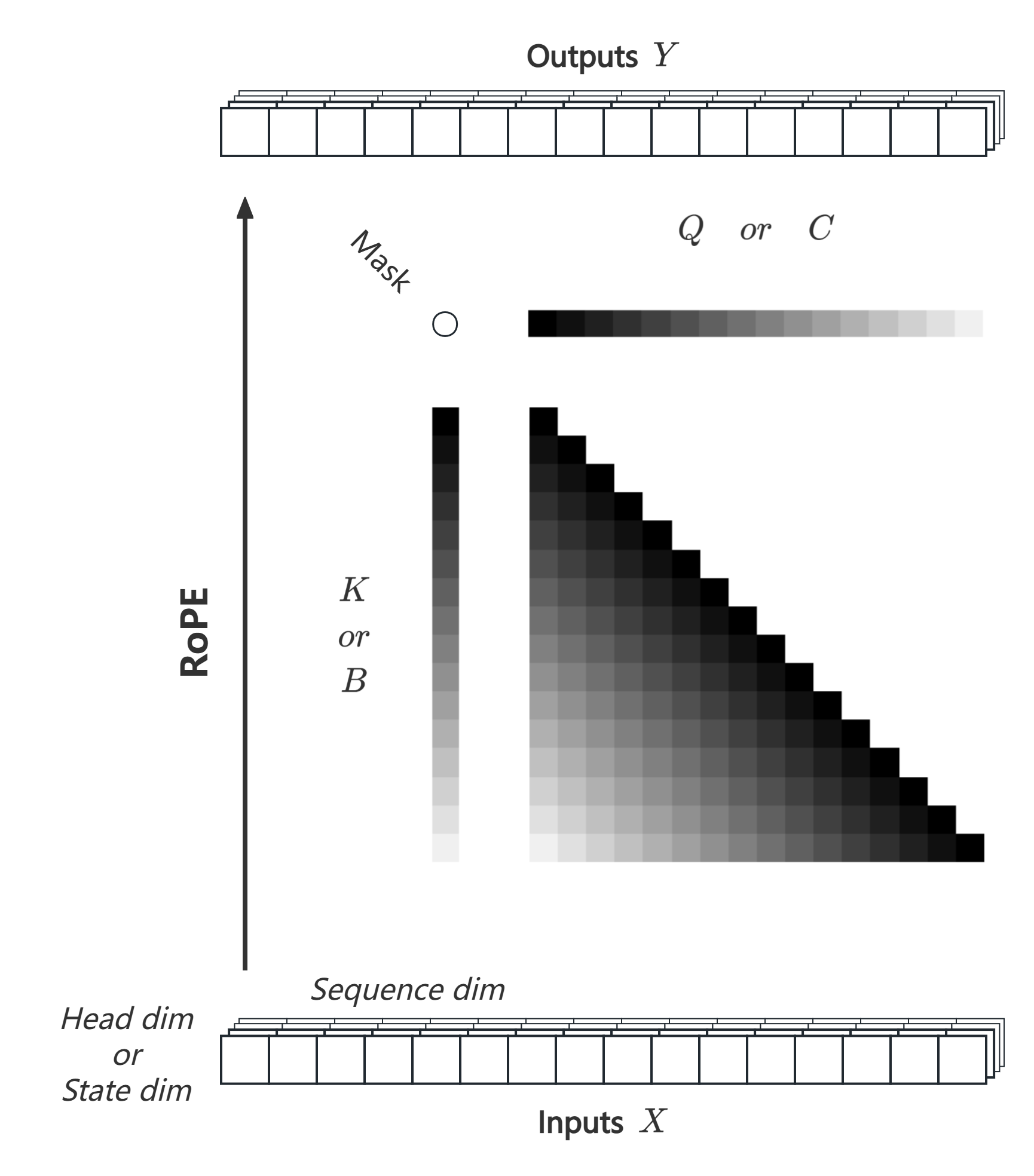
Figure 2: (RoPE.) Shows the algorithm matrix of the rotation position encoding in the form of inner product.

For example, in the self-attention $QK^{\top}$, the dot product of two vectors $Q_{i}\cdot K_{j}$ is calculated, and the result is a scalar, which represents the correlation between position $i$ and position $j$.

The basic idea of rotation position encoding is to encode the position information as a complex rotation matrix, whose angle is determined by the position index. When $QK$ or $CB$ is applied with RoPE, if an element position is close to the front, its rotation will affect the direction of the $K$ or $B$ vector multiplied by it, thereby affecting the result of the inner product.

Define RoPE as $f_{\{Q,K\}}(x_{i},i)$ and $f_{\{C,B\}}(x_{i},i)$, where $x_{i}$ is the input vector, and $i$ is the position index, then:

$$f_{\{Q,K\}}(x_{i},i) =\mathbb{R}_{\Theta,i}^{d}W_{\{Q,K\}}x_{i}$$ (1)

$$f_{\{C,B\}}(x_{i},i) =\mathbb{R}_{\Theta,i}^{d}W_{\{C,B\}}x_{i}$$ (2)

where $\Theta$ and $\mathbb{R}_{\Theta,i}^{d}$ are defined as follows:

$$\Theta=\{\theta_{i}=n^{-2(i-1)/d},i\in[1,2,\dots,d/2]\}$$ (3)

$$\mathbb{R}_{\Theta,i}^{d}=\begin{bmatrix}\cos i\theta_{0}&-\sin i\theta_{0}&0&0&\dots&0&0\\ \sin i\theta_{0}&\cos i\theta_{0}&0&0&\dots&0&0\\ 0&0&\cos i\theta_{1}&-\sin i\theta_{1}&\dots&0&0\\ 0&0&\sin i\theta_{1}&\cos i\theta_{1}&\dots&0&0\\ \vdots&\vdots&\vdots&\vdots&\ddots&\vdots&\vdots\\ 0&0&0&0&\dots&\cos i\theta_{d/2}&-\sin i\theta_{d/2-1}\\ 0&0&0&0&\dots&\sin i\theta_{d/2}&\cos i\theta_{d/2-1}\\ \end{bmatrix}$$ (4)

Table 1: ($Conv1d+D$ vs. $a_{t}$ vs. $RoPE$.) Set the sequence length to 8192. Stacking SSD modules and MLP modules, each accounting for $50\%$. The positional information comes from $Conv1d+D$, $a_{t}$, and $RoPE$, the difference in perplexity performance on the pre-training subset. Stacking SSD modules, Attn modules, and MLP modules, each accounting for $37.5\%$, $12.5\%$, and $50\%$. The difference in perplexity performance on the pre-training subset.

Module	$Conv1d+D$	$a_{t}$	$RoPE$
	ppl $\downarrow$	ppl $\downarrow$	ppl $\downarrow$
SSD + MLP	2.56	2.62	2.33
SSD + Attn + MLP	2.48	2.56	2.18

In Figure 2, the algorithm matrix of the rotation position encoding in the form of inner product is shown. In Appendix A.1, an example of the implementation code of RoPE and the application of RoPE in Attn and SSD is provided.

From Table 1, we can observe that, when the SSD module and the MLP module each account for $50\%$, the best perplexity performance is achieved when the positional information comes from $RoPE$. When the SSD module, the Attn module, and the MLP module each account for $37.5\%$, $12.5\%$, and $50\%$, since the Attn module can only use $RoPE$ as the source of positional information, the improvement in perplexity performance when using $RoPE$ is more significant than when using $Conv1d+D$ and $a_{t}$. The dataset and hyperparameters will be introduced in the following chapters.

4.2 Inner Function Attention

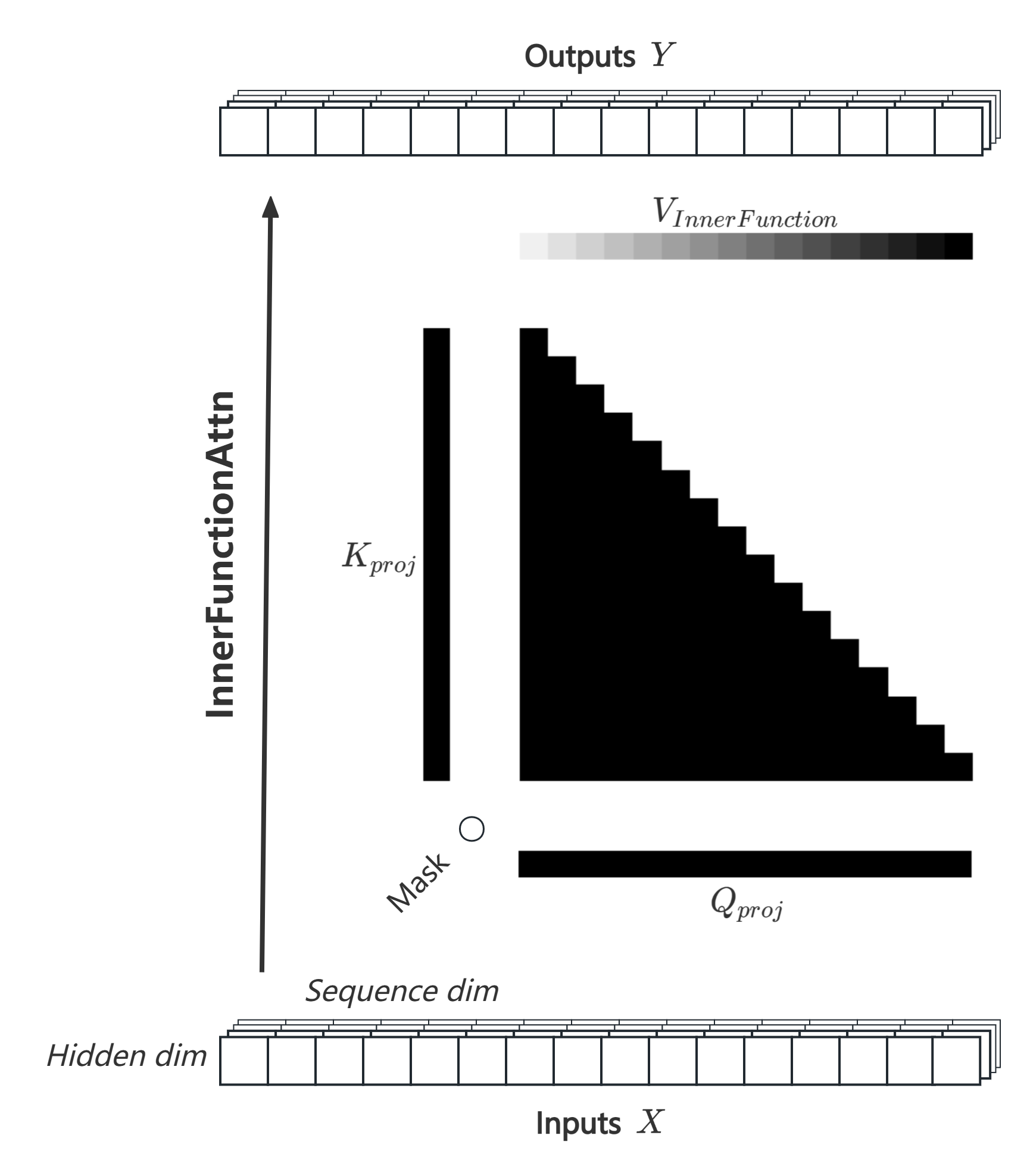
Figure 3: (Inner Function Attention.) Shows the structure and algorithm of inner function attention.

The quadratic self-attention algorithm calculates the $Q$ and $K$ related to the entire input sequence $X$ to form the attention matrix, and the hidden state (usually referred to as the $KV$ cache) is a linearly growing list with $t$ (token), explicitly storing all historical context information without any compression, and the time complexity of calculating this linearly growing state is quadratically increasing, which is a characteristic of quadratic self-attention. I do not consider the efficiency problem of this quadratic algorithm on long sequences $O(t)$ in this paper.

$$Q_{proj} =XW_{Q}$$ (5)

$$K_{proj} =XW_{K}$$ (6)

To improve the expressive power of the quadratic self-attention hidden state from the perspective of ignoring a certain speed to improve the effect, and finally achieve efficiency improvement, it is necessary to change from a simple $y=xW$ to an excellent heuristic $y=f(x,W,...)$. Considering that $Q$ and $K$ need to perform inner product operations, more complex operations may cause large fluctuations during training, so the heuristic should be applied to $V$. Of course, from a more intuitive perspective, queries and keys do indeed only need simple linear transformations, and their dot product similarity, that is, the attention matrix, is to determine which information to extract from the values. Therefore, we can apply the heuristic to the values to improve the expressive power of the hidden state. This is the basic idea of inner function attention.

$$V_{InnerFunction}=f(X,W,...)$$ (7)

Suppose there is a Super Hero with a photographic memory, who can remember everything seen and recall any detail. When you ask it a question, at first, you will decide that this Super Hero is very smart and seems to know everything. But as you ask more and more questions, you will realize that it does not think at all because it refuses to compress information and cannot extract patterns and rules from a large amount of information. Having the ability to compress information in both training and reasoning is the key to intelligence.

In OTCE [11], it was found that when mixing SSM [4] with Attention, if the entire sequence is calculated, the quadratic self-attention algorithm can learn the recursive state update from $h_{t-1}$ to $h_{t}$. And the state space algorithm such as SSD [2] has a constant state size, using it as a heuristic will not cause too much speed reduction on long sequences. So $V=SSD(X,W_{A},W_{B},W_{C})$ is a selective recursive state related to the input $X$, from $h_{0}$ to $h_{t}$, which meets the requirements of improving the expressive power of the hidden state.

$$V_{InnerFunction}=SSD(X,W_{A},W_{B},W_{C})$$ (8)

Then the attention matrix calculated by $QK^{T}$ extracts information from the selective recursive state $V$, retaining the explicit storage of all historical context information of the quadratic self-attention.

$$A =softmax(Q_{proj}K_{proj}^{T})$$ (9)

$$Y =AV_{InnerFunction}$$ (10)

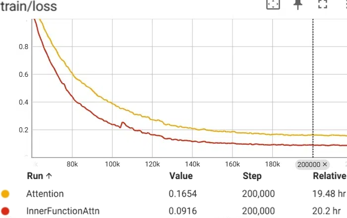
Figure 4: (Inner Function Attn vs. Attention.) Set the sequence length to 8192. Stacking SSD modules, Attn modules, and CDMMOE modules, each accounting for $37.5\%$, $12.5\%$, and $50\%$, the parameter is 1.3B. The loss curve of the two different quadratic self-attention algorithms on the fine-tuning training set.

In Figure 3, the algorithm matrix of inner function attention is shown. In Appendices A.2 and A.3, an example of the implementation code of SSD and the application of SSD as a heuristic for inner function attention is provided.

From Figure 4, we can observe that, with almost the same model parameter, the loss curve of Inner Function Attn is reduced by more than $40\%$ compared to the loss curve of Attention. Of course, the speed of Inner Function Attn is about $4\%$ slower than Attention. The dataset and hyperparameters will be introduced in the following chapters.

4.3 Cross Domain Million Mixture of Experts

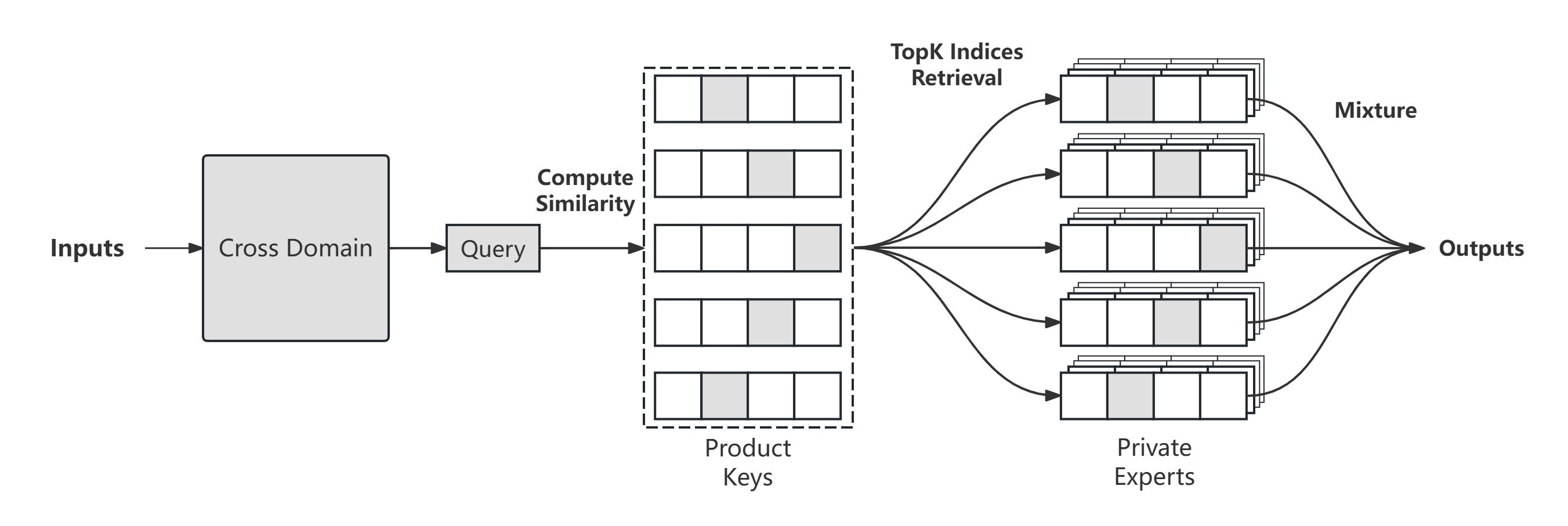
Figure 5: (CDMMOE.) Shows the internal structure and calculation process of the cross domain million mixture of experts matrix.

In the conventional mixture of experts strategy, the tokens assigned to different experts need to have common knowledge or information, so multiple experts will have redundant parameters for storing common information when obtaining their respective parameters, which leads to expert parameter redundancy. And the proportion of expert parameter redundancy increases with the increase in expert granularity and the decrease in the number of expert activations. In Mixture of A Million Experts (MMOE) [5], due to the high degree of expert refinement, the proportion of expert parameter redundancy reaches an astonishingly high level, which can be seen in the loss curve at the beginning of pre-training.

However, if the tokens assigned to different experts have already passed through the parameters for storing common knowledge, the parameter redundancy can be reduced. The reduction of redundancy will help build a more efficient and professional mixture of experts. This parameter for storing common knowledge can be called cross-domain.

$$CrossDomain(x,W^{s},V^{s},W_{2}^{s}) =(xW^{s}\cdot\sigma(xV^{s}))W_{2}^{s}$$ (11)

where $s$ represents shared parameters, $\sigma$ represents the activation function, $W,V,W_{2}$ represent the three weight matrices of the Gated MLP.

Subsequently, we use the output of the cross-domain as the input of the private mixture of experts, where the mixture of experts strategy can be a classic routing strategy or the PEER [5] strategy.

$$f(x) =\sum_{i=1}^{N}e_{i}^{p}(CrossDomain(x))$$ (12)

where $e$ represents the expert, $p$ represents the private parameters, and $N$ represents the number of experts.

Of course, in order to allow private experts to decide for themselves which information from the shared cross-domain should be used and to be able to arbitrarily adjust the proportion of shared cross-domain parameters, it is necessary to make certain modifications to the PEER strategy. Taking only one private expert as an example:

$$In\_Private(x,W) =CrossDomain(x)W\quad W\in\mathbb{R}^{d^{s}\times d^{p}}$$ (13)

$$CDMMOE(x,W^{p},V^{p},W_{2}^{p}) =(xW^{p\ T}\cdot\sigma(xV^{p\ T}))W_{2}$$ (14)

This algorithm with the ability to arbitrarily adjust the shared cross-domain parameters and combined with the PEER strategy as private experts, I call it Cross Domain Million Mixture of Experts (CDMMOE). Compared to CDMOE [11], it can expand the number of experts 1024 times (from 4 to 4096) under the same shared dimension (4096) and private dimension (2048) while maintaining the same number of parameters, and the speed has slightly improved.

In Figure 5, the internal structure and calculation process of the cross-domain million mixture of experts matrix are shown. In Appendix A.4, an example of the implementation code of CDMMOE is provided.

4.4 Cheems Architecture

In fact, after the discussion of the previous few sections, the architecture of Cheems has emerged. I use RoPE in the inner product positional encoding as the source of positional information for SSD and Attn. Add a CDMMOE module after each SSD or InnerFunctionAttn module to store factual knowledge. Considering that the quadratic self-attention is slow in long sequence calculation, more SSD modules are needed to extend the model depth. Considering the selective nature of SSD, the SSD module is used before the InnerFunctionAttn module for information filtering. Considering that the SSD module at the end of the model will lead to knowledge routing bias within a certain range, the SSD module is not used at the end of the model. There are many studies that show that the best perplexity performance of the model is when the ratio of SSD to Attn is 7:1. Therefore, a Cheems module is $7\times(\text{RoPE}+\text{SSD}+\text{CDMMOE})+(\text{RoPE}+\text{InnerFunctionAttn}+\text{CDMMOE})$, stacked in this way.

5 Empirical Validation

5.1 Environment Dataset and Hyperparameters

• The environment is an open-source PyTorch image provided by Nvidia [10].

• The pre-training dataset is a mixture of open-source datasets including Book, Wikipedia, UNCorpus, translation2019zh, WikiMatri, news-commentry, ParaCrawlv9, ClueCorpusSmall, CSL, news-crawl, etc.

• The SFT fine-tuning is 2 million instructions of the Belle dataset.

• Use the Trainer class of the Transformers library for training and evaluation and save relevant metrics.

• Use GLM [3] as the architecture backbone.

• The $AdamW$ hyperparameters are set to $\beta_{1}=0.9,\beta_{2}=0.98,\epsilon=10^{-6}$.

• The linear warm-up steps are $10\%$ of the total steps, reaching the maximum learning rate of 2e-4, and then cosine decay to the minimum learning rate of 2e-5.

• Use $RMSNorm$ instead of $LayerNorm$.

• No linear bias terms.

5.2 Language Modeling

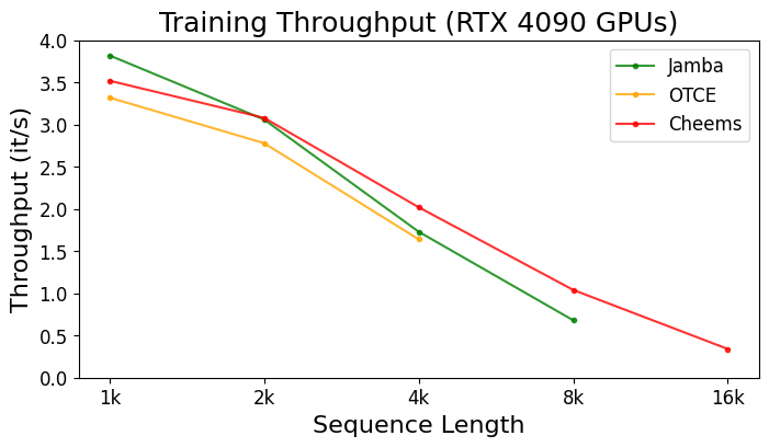
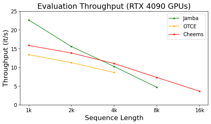
Figure 6: (Efficiency Benchmark.) Three architectures of mixed state space and attention: Jamba, OTCE, and Cheems. (Left) Throughput during training of Jamba-1.3B, OTCE-1.3B, and Cheems-1.3B. Cheems surpasses the other two architectures when the sequence length is 2K, and its advantage becomes more pronounced as the sequence length increases. (Right) Throughput during evaluation of Jamba-1.3B, OTCE-1.3B, and Cheems-1.3B. Cheems surpasses the other two architectures when the sequence length is 4K, and its advantage becomes more pronounced as the sequence length increases.

Table 2: (Effectiveness Benchmark.) Three architectures of mixed state space and attention: Jamba, OTCE, and Cheems. When the parameter is 280M, the perplexity performance of pre-training and fine-tuning of the three architectures and the verification accuracy in CLUE [15] are compared. When the parameter is 1.3B, the perplexity performance of pre-training and fine-tuning of the three architectures and the verification accuracy in CLUE, CEval [6], PIQA [1], NarrativeQA [8], HotpotQA [16] are compared. Cheems performs best in almost all metrics.

Model	PreTrain	FineTune	CLUE	CEval	PIQA	NarrativeQA	HotpotQA	Average
	ppl $\downarrow$	ppl $\downarrow$	acc $\uparrow$	acc $\uparrow$	acc $\uparrow$	acc $\uparrow$	acc $\uparrow$	acc $\uparrow$
Jamba-280M	2.53	1.98	75.89	—	—	—	—	75.89
OTCE-280M	2.10	1.46	79.12	—	—	—	—	79.12
Cheems-280M	2.12	1.32	80.82	—	—	—	—	80.82
Jamba-1.3B	2.12	1.66	82.12	42.05	78.65	23.15	34.40	52.07
OTCE-1.3B	1.88	1.28	89.02	46.86	79.48	27.98	42.71	57.21
Cheems-1.3B	1.45	1.08	92.33	49.18	79.23	29.82	45.32	59.18

The architecture of mixed state space algorithm and attention algorithm naturally needs to be compared with the same hybrid architecture, I chose Jamba [9] and OTCE [11] as the comparison objects.

In Figure 6, the throughput during training (forward pass and backward pass) and evaluation (forward propagation) of the three architectures is shown. Cheems architecture shows higher efficiency when the sequence length is above 4K in modern large-scale language modeling.

In Table 2, the perplexity performance of pre-training and fine-tuning of the three architectures at different scales and the verification accuracy on different tasks are compared. Cheems shows extremely low perplexity performance in SFT fine-tuning. CLUE is the benchmark for evaluating the model’s performance on sequence classification tasks. CEval is the benchmark for evaluating the model’s comprehensive ability on many domains, more detailed performance on each subtask is shown in Appendix B.1. PIQA (standard short context task), NarrativeQA (natural long context task), and HotpotQA (synthetic long context task) are benchmarks for evaluating the model’s associative memory recall performance at different context lengths, Cheems shows better performance as the context length increases.

6 Conclusion

This paper explores and proposes a new basic model architecture Cheems, continuing to promote language modeling in a more efficient and more effective direction.

Appendix A Implementation Code

A.1 RoPE

[!ht]

⬇

class RotaryEmbedding:

def __init__(self, dim, max_position_embeddings, base=10000, scaling_factor=1.0):

self.dim = dim

self.max_position_embeddings = max_position_embeddings

self.base = base

self.scaling_factor = scaling_factor

inv_freq = 1.0 / (self.base ** (torch.arange(0, self.dim, 2) / self.dim))

self.register_buffer("inv_freq", inv_freq)

def forward(self, x, position_ids):

seq_len = torch.max(position_ids) + 1

if seq_len > self.max_position_embeddings:

base = self.base * (

(self.scaling_factor * seq_len / self.max_position_embeddings) - (self.scaling_factor - 1)

) ** (self.dim / (self.dim - 2))

inv_freq = 1.0 / (

base ** (torch.arange(0, self.dim, 2) / self.dim)

)

else:

inv_freq = self.inv_freq

inv_freq_expanded = inv_freq[None, :, None].expand(position_ids.shape[0], -1, 1)

position_ids_expanded = position_ids[:, None, :]

freqs = (inv_freq_expanded @ position_ids_expanded).transpose(1, 2)

emb = torch.cat((freqs, freqs), dim=-1)

cos = emb.cos().to(x.dtype)

sin = emb.sin().to(x.dtype)

return cos, sin

def rotate_half(x):

x1 = x[…, : x.shape[-1] // 2]

x2 = x[…, x.shape[-1] // 2 :]

return torch.cat((-x2, x1), dim=-1)

def apply_QK_rotary_pos_emb(q, k, cos, sin, unsqueeze_dim=2):

cos = cos.unsqueeze(unsqueeze_dim)

sin = sin.unsqueeze(unsqueeze_dim)

q_embed = (q * cos) + (rotate_half(q) * sin)

k_embed = (k * cos) + (rotate_half(k) * sin)

return q_embed, k_embed

def apply_BC_rotary_pos_emb(b, c, cos, sin, unsqueeze_dim=2):

cos = cos.unsqueeze(unsqueeze_dim)

sin = sin.unsqueeze(unsqueeze_dim)

b_embed = (b * cos) + (rotate_half(b) * sin)

c_embed = (c * cos) + (rotate_half(c) * sin)

return b_embed, c_embed

PyTorch example of RoPE.

A.2 SSD

[!ht]

⬇

class SSD:

def __init__(self, hidden_dim, num_ssd_heads, ssd_state_dim, max_position_embeddings):

self.hidden_dim = hidden_dim

self.num_ssd_heads = num_ssd_heads

self.ssm_head_dim = self.hidden_dim // self.num_ssd_heads

self.ssd_state_dim = ssd_state_dim

# State Space Dual Linear Projections and Parameters

self.X_proj = Linear(self.hidden_dim, self.hidden_dim)

self.A_log = Parameter(torch.log(torch.ones(self.num_ssd_heads)))

self.B_proj = Linear(self.hidden_dim, self.ssd_state_dim * self.num_ssd_heads)

self.C_proj = Linear(self.hidden_dim, self.ssd_state_dim * self.num_ssd_heads)

self.dt_proj = Linear(self.hidden_dim, self.num_ssd_heads)

self.out_proj = Linear(self.hidden_dim, self.hidden_dim)

# Rotary Position Embedding

self.BC_rotary_emb = RotaryEmbedding(self.ssd_state_dim, max_position_embeddings)

def forward(self, hidden_states, position_ids):

"""

Arguments: hidden_states: (batch, length, hidden_dim)

Return: hidden_states: (batch, length, hidden_dim)

Notation:

b - batch

t - length

d - hidden dim

h - heads

p - head dim

n - ssd state dim

"""

# Compute State Space Dual Parameters

X = self.X_proj(hidden_states)

A = -torch.exp(self.A_log)

B = self.B_proj(hidden_states)

C = self.C_proj(hidden_states)

dt = self.dt_proj(hidden_states)

# Split into multiple heads

X = rearrange(X, "b t (h p) -> b t h p", h=self.num_ssd_heads)

B = rearrange(B, "b t (h n) -> b t h n", h=self.num_ssd_heads)

C = rearrange(C, "b t (h n) -> b t h n", h=self.num_ssd_heads)

# Apply rotary position embedding to B and C

cos, sin = self.BC_rotary_emb(hidden_states, position_ids=position_ids)

B, C = apply_BC_rotary_pos_emb(B, C, cos, sin)

# Compute State Space Dual matrix and rotary position encoding matrix weighted to X

Y = rearrange(mamba_chunk_scan_combined(

X,

A,

B,

C,

dt

), "b t h p -> b t (h p)")

# Project Output

out = self.out_proj(Y)

return out

PyTorch example of SSD. For simplicity, the $mamba\_chunk\_scan\_combined$ function from the mamba-ssm library is not included.

A.3 SSD-Attn

[!ht]

⬇

class SSDAttn:

def __init__(self, hidden_dim, num_attn_heads, max_position_embeddings):

self.hidden_dim = hidden_dim

self.num_attn_heads = num_attn_heads

self.attn_head_dim = self.hidden_dim // self.num_attn_heads

# Attntion Linear Projections

self.Q_proj = Linear(hidden_dim, self.attn_head_dim * num_attn_heads)

self.K_proj = Linear(hidden_dim, self.attn_head_dim * num_attn_heads)

self.out_proj = Linear(hidden_dim, hidden_dim)

# Inner Function

self.V_layer = SSD(hidden_dim, …)

# Rotary Position Embedding

self.QK_rotary_emb = RotaryEmbedding(self.attn_head_dim, max_position_embeddings)

def forward(self, hidden_states, attn_mask, position_ids):

"""

Arguments: hidden_states: (batch, length, hidden_dim)

Return: hidden_states: (batch, length, hidden_dim)

Notation:

b - batch

t - length

d - hidden dim

h - heads

p - head dim

"""

# Compute linear projection Q K and inner function V

Q = self.Q_proj(hidden_states)

K = self.K_proj(hidden_states)

V = self.V_layer(hidden_states, position_ids=position_ids)

# Split into multiple heads

Q = rearrange(Q, "b t (h p) -> b t h p", h=self.num_attn_heads)

K = rearrange(K, "b t (h p) -> b t h p", h=self.num_attn_heads)

V = rearrange(V, "b t (h p) -> b t h p", h=self.num_attn_heads)

# Apply rotary position embedding to Q and K

cos, sin = self.QK_rotary_emb(V, position_ids=position_ids)

Q, K = apply_QK_rotary_pos_emb(Q, K, cos, sin)

# Compute Attention score matrix and rotary position encoding matrix weighted to inner function state V

attn = rearrange(scaled_dot_product_attention(

rearrange(Q, "b t h p -> b h t p"),

rearrange(K, "b t h p -> b h t p"),

rearrange(V, "b t h p -> b h t p"),

attn_mask=attn_mask

), "b h t p -> b t (h p)")

# Project Output

out = self.out_proj(attn)

return out

PyTorch example of SSD-Attn. For simplicity, the $scaled\_dot\_product\_attention$ function from the pytorch library is not included.

A.4 Cross Domain Million Mixture of Experts

[!ht]

⬇

class CDMMOE:

def __init__(self, hidden_dim, hidden_act, shared_intermediate_dim, private_intermediate_dim, num_heads, num_experts, num_experts_per_head):

self.act_fn = ACT2FN[hidden_act]

# Shared Domain

self.shared_gate_proj = Linear(hidden_dim, shared_intermediate_dim)

self.shared_up_proj = Linear(hidden_dim, shared_intermediate_dim)

self.shared_down_proj = Linear(shared_intermediate_dim, hidden_dim)

# Linear projection into private experts

self.in_private_proj = Linear(hidden_dim, private_intermediate_dim)

# Queries and Keys

self.queries = Sequential(

Linear(private_intermediate_dim, private_intermediate_dim // 2 * num_heads * 2),

Rearrange(’b t (p h d) -> p b t h d’, p = 2, h = num_heads)

)

self.num_keys = int(math.sqrt(num_experts))

self.keys = nn.Parameter(torch.zeros(num_heads, self.num_keys, 2, private_intermediate_dim // 2))

self.num_experts_per_head = num_experts_per_head

# Private Experts

self.gate_embed = Embedding(num_experts, private_intermediate_dim)

self.up_embed = Embedding(num_experts, private_intermediate_dim)

self.down_embed = Embedding(num_experts, hidden_dim)

def forward(self, hidden_states):

"""

Arguments: hidden_states: (batch, length, hidden_dim)

Return: hidden_states: (batch, length, hidden_dim)

Notation:

b - batch

t - length

d - hidden dim

h - heads

p - 2 for product key

k - number of keys

"""

# Compute Shared Domain

hidden_states = self.shared_down_proj(self.shared_up_proj(hidden_states) * self.act_fn(self.shared_gate_proj(hidden_states)))

# Project into Private Experts

hidden_states = self.in_private_proj(hidden_states)

# Queries and Keys for Product-Key

queries = self.queries(hidden_states)

sim = torch.einsum(’p b t h d, h k p d -> p b t h k’, queries, self.keys)

(scores_x, scores_y), (indices_x, indices_y) = sim.topk(self.num_experts_per_head, dim=-1)

all_scores = einx.add(’… i, … j -> … (i j)’, scores_x, scores_y)

all_indices = einx.add(’… i, … j -> … (i j)’, indices_x * self.num_keys, indices_y)

scores, pk_indices = all_scores.topk(self.num_experts_per_head, dim=-1)

indices = all_indices.gather(-1, pk_indices)

# Compute Private Experts

gate_embed = self.gate_embed(indices)

up_embed = self.up_embed(indices)

down_embed = self.down_embed(indices)

gate = torch.einsum(’b t d, b t h k d -> b t h k’, hidden_states, gate_embed)

hidden_states = torch.einsum(’b t d, b t h k d -> b t h k’, hidden_states, up_embed)

hidden_states = hidden_states * self.act_fn(gate) * scores.softmax(dim=-1)

return torch.einsum(’b t h k, b t h k d -> b t d’, hidden_states, down_embed)

PyTorch example of CDMMOE.

Appendix B Comparative

B.1 Mixture of Experts

Table 3: (Jamba vs. OTCE vs. Cheems in CEvalBenchmark.) These tasks come from CEvalBenchmark [6], I detail the zero-shot and five-shot accuracy of the three sparse activation mixture of experts architectures on each subtask.

Task	Jamba	OTCE	Cheems	Jamba	OTCE	Cheems
	zero-shot $\uparrow$	zero-shot $\uparrow$	zero-shot $\uparrow$	five-shot $\uparrow$	five-shot $\uparrow$	five-shot $\uparrow$
computer network	45.65	53.51	55.63	48.23	54.87	56.81
operating system	54.42	60.11	61.65	54.42	51.41	52.02
computer architecture	55.34	54.21	56.33	55.34	52.09	56.56
college programming	34.90	36.36	39.65	35.03	36.36	39.08
college physics	41.48	37.65	43.15	41.01	43.15	43.15
college chemistry	23.76	44.37	56.86	46.11	61.34	62.52
advanced mathematics	42.23	43.76	47.76	44.44	47.76	48.12
probability and statistics	45.66	45.66	42.12	38.17	41.21	44.85
discrete mathematics	37.85	44.44	40.56	37.85	39.57	41.42
electrical engineer	38.75	42.55	45.52	42.55	51.34	54.76
metrology engineer	37.61	36.45	40.02	38.18	39.98	45.32
high school mathematics	42.21	44.44	45.78	43.01	44.44	46.02
high school physics	51.84	55.88	56.34	47.41	50.31	55.68
high school chemistry	23.72	54.54	56.78	24.14	54.54	57.05
high school biology	48.76	48.76	48.38	50.18	56.54	57.32
middle school mathematics	62.59	65.76	66.12	62.07	65.76	66.45
middle school biology	37.82	38.10	37.82	37.82	38.10	38.78
middle school physics	59.87	59.87	60.86	47.32	48.76	54.78
middle school chemistry	43.32	45.00	52.14	43.32	43.32	50.67
veterinary medicine	46.31	51.11	52.24	46.31	51.78	52.98
college economics	23.17	34.87	32.45	25.56	31.23	34.87
business administration	35.51	34.44	34.44	37.11	41.21	43.76
marxism	48.99	54.67	57.02	52.06	57.43	58.91
mao zedong thought	9.87	25.00	32.10	12.12	24.43	32.10
education science	31.77	33.43	32.72	32.11	34.32	34.32
teacher qualification	28.67	29.98	28.67	29.89	32.77	34.33
high school politics	66.12	65.47	68.63	66.12	68.98	72.16
high school geography	53.21	53.21	53.21	52.88	53.21	53.73
middle school politics	34.54	38.10	39.02	32.23	37.81	40.68
middle school geography	68.43	71.10	68.89	44.35	45.78	60.18
modern chinese history	47.34	46.43	54.91	60.55	62.12	64.56
ideological and moral cultivation	24.76	45.55	47.75	27.17	42.21	45.55
logic	54.55	54.55	54.55	52.86	54.55	53.65
law	43.63	47.76	48.74	46.11	52.32	53.27
chinese language and literature	52.43	55.55	56.89	52.14	55.55	58.65
art studies	32.11	31.21	30.99	32.11	34.44	32.75
professional tour guide	48.47	49.87	50.12	45.78	45.78	48.74
legal professional	46.97	53.43	53.43	48.56	56.66	56.18
high school chinese	45.56	45.56	49.60	46.06	48.64	58.58
high school history	32.33	45.00	45.00	41.24	55.00	56.55
middle school history	51.67	49.94	51.67	43.88	45.77	51.67
civil servant	31.06	30.76	32.82	32.35	34.77	33.04
sports science	34.66	45.54	56.14	57.42	70.12	62.68
plant protection	41.66	45.88	44.72	40.68	45.88	44.08
basic medicine	60.01	65.67	65.67	55.55	61.32	62.85
clinical medicine	40.91	50.00	52.55	36.24	40.91	45.74
urban and rural planner	37.51	41.30	38.88	38.02	41.30	39.48
accountant	21.66	32.44	36.53	23.33	34.34	36.53
fire engineer	31.21	30.32	35.25	33.44	37.75	38.79
environmental impact assessment	36.66	46.56	46.56	36.25	46.56	46.56
tax accountant	25.92	34.69	42.11	25.15	32.65	38.02
physician	29.55	35.32	36.02	32.86	38.78	40.32
Average	41.25	45.88	47.76	42.05	46.86	49.18

References

- [1] Yonatan Bisk, Rowan Zellers, Jianfeng Gao and Yejin Choi “PIQA: Reasoning about Physical Commonsense in Natural Language” In Proceedings of the AAAI conference on Artificial Intelligence 34, 2020
- [2] Tri Dao and Albert Gu “Transformers are SSMs: Generalized Models and Efficient Algorithms Through Structured State Space Duality” In International Conference on Machine Learning (ICML), 2024
- [3] Zhengxiao Du, Yujie Qian, Xiao Liu, Ming Ding, Jiezhong Qiu, Zhilin Yang and Jie Tang “GLM: General Language Model Pretraining with Autoregressive Blank Infilling” In Proceedings of the 60th Annual Meeting of the Association for Computational Linguistics (Volume 1: Long Papers), 2022, pp. 320–335
- [4] Albert Gu and Tri Dao “Mamba: Linear-Time Sequence Modeling with Selective State Spaces” In arXiv preprint arXiv:2312.00752, 2023
- [5] Xu Owen He “Mixture of A Million Experts” In arXiv preprint arXiv:2407.04153, 2024
- [6] Yuzhen Huang, Yuzhuo Bai, Zhihao Zhu, Junlei Zhang, Jinghan Zhang, Tangjun Su, Junteng Liu, Chuancheng Lv, Yikai Zhang, Jiayi Lei, Yao Fu, Maosong Sun and Junxian He “C-Eval: A Multi-Level Multi-Discipline Chinese Evaluation Suite for Foundation Models” In Advances in Neural Information Processing Systems, 2023
- [7] Angelos Katharopoulos, Apoorv Vyas, Nikolaos Pappas and François Fleuret “Transformers are RNNs: Fast Autoregressive Transformers with Linear Attention” In International Conference on Machine Learning, 2020, pp. 5156–5165 PMLR
- [8] Tomas Kovcisky, Bryan McCann, James Bradbury, Caiming Xiong and Richard Socher “The NarrativeQA Reading Comprehension Challenge” In Transactions of the Association for Computational Linguistics 6, 2018, pp. 317–328
- [9] Opher Lieber, Barak Lenz, Hofit Bata, Gal Cohen, Jhonathan Osin, Itay Dalmedigos, Erez Safahi, Shaked Meirom, Yonatan Belinkov and Shai Shalev-Shwartz “Jamba: A Hybrid Transformer-Mamba Language Model” In arXiv preprint arXiv:2403.19887, 2024
- [10] Meta NVIDIA “PyTorch Container Image”, https://catalog.ngc.nvidia.com/orgs/nvidia/containers/pytorch, 2022
- [11] Jingze Shi, Ting Xie, Bingheng Wu, Chunjun Zheng and Kai Wang “OTCE: Hybrid SSM and Attention with Cross Domain Mixture of Experts to construct Observer-Thinker-Conceiver-Expresser” In arXiv preprint arXiv:2406.16495, 2024
- [12] Jianlin Su, Yu Lu, Shengfeng Pan, Ahmed Murtadha, Bo Wen and Yunfeng Liu “Roformer: Enhanced Transformer with Rotary Position Embedding” In arXiv preprint arXiv:2104.09864, 2021
- [13] Yu Sun, Xinhao Li, Karan Dalal, Jiarui Xu, Arjun Vikram, Genghan Zhang, Yann Dubois, Xinlei Chen, Xiaolong Wang, Sanmi Koyejo, Tatsunori Hashimoto and Carlos Guestrin “Learning to (Learn at Test Time): RNNs with Expressive Hidden States” In arXiv preprint arXiv:2407.04620, 2024
- [14] Ashish Vaswani, Noam Shazeer, Niki Parmar, Jakob Uszkoreit, Llion Jones, Aidan N. Gomez, Lukasz Kaiser and Illia Polosukhin “Attention is All You Need” In arXiv preprint arXiv:1706.03762, 2017
- [15] Liang Xu, Hai Hu, Xuanwei Zhang, Lu Li, Chenjie Cao, Yudong Li, Yechen Xu, Kai Sun, Dian Yu, Cong Yu, Yin Tian, Qianqian Dong, Weitang Liu, Bo Shi, Yiming Cui, Junyi Li, Jun Zeng, Rongzhao Wang, Weijian Xie, Yanting Li, Yina Patterson, Zuoyu Tian, Yiwen Zhang, He Zhou, Shaoweihua Liu, Zhe Zhao, Qipeng Zhao, Cong Yue, Xinrui Zhang, Zhengliang Yang, Kyle Richardson and Zhenzhong Lan “CLUE: A Chinese Language Understanding Evaluation Benchmark” In Proceedings of the 28th International Conference on Computational Linguistics Barcelona, Spain (Online): International Committee on Computational Linguistics, 2020, pp. 4762–4772 DOI: 10.18653/v1/2020.coling-main.419
- [16] Zhilin Yang, Peng Qi, Saizheng Zhang, Yoshua Bengio, William W Cohen, Ruslan Salakhutdinov and Christopher D Manning “HotpotQA: A Dataset for Diverse, Explainable Multi-hop Question Answering” In arXiv preprint arXiv:1809.09600, 2018