Real-time risk estimation for active road safety: Leveraging Waymo AV sensor data with hierarchical Bayesian extreme value models

Abstract

This study develops a real-time framework for estimating the risk of near-misses by using high-fidelity two-dimensional (2D) risk indicator time-to-collision (TTC), which is calculated from high-resolution data collected by autonomous vehicles (AVs). The framework utilizes extreme value theory (EVT) to derive near-miss risk based on observed TTC data. Most existing studies employ a generalized extreme value (GEV) distribution for specific sites and conflict types and often overlook individual vehicle dynamics heterogeneity. This framework is versatile across various highway geometries and can encompass vehicle dynamics and fidelity by incorporating covariates such as speed, acceleration, steering angle, and heading. This makes the risk estimation framework suitable for dynamic, real-world traffic environments. The dataset for this study is derived from Waymo perception data, encompassing six sites across three cities: San Francisco, Phoenix, and Los Angeles. Vehicle trajectory data were extracted from the dataset, and near-miss frequencies were calculated using high-fidelity 2D TTC. The crash risk was derived from observed near misses using four hierarchical Bayesian GEV models, explicitly focusing on conflicting pairs as block minima (BM), which revealed that crash risk varies across pairs. The proposed framework is efficient using a hierarchical Bayesian structure random parameter (HBSRP) model, offering superior statistical performance and flexibility by accounting for unobserved heterogeneity across sites. The study identifies and quantifies that the most hazardous conditions involve conflicting vehicle speeds and rapid acceleration and deceleration, significantly increasing crash risk in urban arterials. This finding underscores the importance of incorporating vehicular dynamic covariates heterogeneity in risk assessment, which bridges the gap between active and passive safety measures. The proposed methodology can be utilized for more accurate risk assessment in heterogeneous traffic, providing valuable insights for improving road safety in diverse environments.

1 Introduction

Ensuring highway safety is paramount to maintaining the integrity of our transportation systems and achieving vision zero. In 2021, there were 39,508 fatal crashes, resulting in a fatality rate of 1.37 per 100 million vehicle miles traveled (VMT), illustrating the seriousness of the issue (NHTSA, 2021). The economic burden is equally staggering, with road crashes costing $498.3 billion annually (National Safety Council, 2021). These statistics underscore the urgent need for robust safety measures, which are vital for individual well-being and societal harmony. As our transportation networks become more complex, ensuring highway safety requires increased attention and investment to protect lives and reduce economic losses.

Furthermore, highway safety reflects the efficiency and reliability of our transportation system, influenced by factors such as infrastructure integrity, driver vigilance, and vehicle standards. However, human error still accounts for 94% of all road crashes, making it the predominant factor (Zhu et al., 2023; Yue et al., 2018; Singh, 2018). This necessitates a more rigorous analysis of human driving behavior, including speed, acceleration, deceleration, steering angle control, braking, etc. With the increased traffic density on urban roads, innovative solutions such as connected and autonomous vehicles (CAVs) are becoming increasingly popular. CAVs have significant potential to enhance highway safety by improving perception, rapidly responding to ambient traffic changes, and eliminating driver distraction and fatigue (Dai et al., 2023). However, awareness among drivers and patterns of behavior remains crucial despite these technological enhancements, especially as CAVs and human-driven vehicles (HDVs) are expected to coexist on our roads for a very long time.

Traditional safety measures often rely on historical aggregated crash data to predict future extreme events within specific roadway entities, widely known as the reactive approach (Arun et al., 2021; Lee et al., 2017; Pei et al., 2011). However, this method has significant drawbacks (Lord et al., 2021), such as the rarity of crashes, the lengthy time needed for crash data collection (Mannering et al., 2020), and the inherent issues with historical data accuracy due to under-reporting and subjective reporting (Arun et al., 2021; Tarko, 2018a). These limitations hinder the ability to make precise facility-specific crash risk predictions and comprehensive safety assessments (Tarko, 2018b; Mannering et al., 2016), and they fail to account for potential crashes, thereby stalling advancements in highway safety research (Wang et al., 2021). To address these issues, an effective alternative involves utilizing near-miss data, which occur much more frequently than actual crashes, and providing an enriched dataset for robust analysis. This approach offers valuable insights into the performance of road networks through vehicle interactions (Tarko, 2018a; Davis et al., 2011). Researchers can develop more proactive and accurate safety interventions by concentrating on near-miss data, thereby significantly advancing highway safety research and its application. This method heavily relies on surrogate safety measures (SSMs) to quantify and analyze these near-miss events.

Although SSMs are commonly employed for analyzing near-miss events, their usefulness in real-world situations is constrained by their dependence on one-dimensional (1D) or longitudinal movement risk (Dai et al., 2023; Das et al., 2022; Rahman and Abdel-Aty, 2018) limits their capacity in real-world scenarios. When a vehicle interacts with its surroundings, such as other vehicles, road objects, and road boundaries, particularly during maneuvers like merging, lane changes, and passing, it is essential to consider both its lateral and longitudinal movement. The complexity of these interactions increases in various scenarios, such as diversions, work zones, and intersections, where the probability of conflicts rises. Although some studies (Lu et al., 2022; Zhang et al., 2020; St-Aubin et al., 2013) have begun to consider both longitudinal and lateral vehicle movements, recent reviews (Wang et al., 2021) have raised concerns about the ability of SSMs to accurately and objectively characterize different traffic facilities. These concerns highlight the need for a comprehensive and high-fidelity analytical framework that is generic and applicable to various scenarios. For this response, Li et al.(2024) developed a 2D risk indicator TTC that would ensure a more accurate representation of complex traffic dynamics, enhancing the capability to predict and mitigate traffic conflicts effectively.

SSM-based near-miss risk studies have traditionally relied on infrastructure-based technologies such as video cameras, lidars, radars, and loop detectors along roadsides. These systems monitor and report time-based traffic parameters like speed, acceleration, and volume within their detection range. However, infrastructure-based systems like roadside cameras and loop detectors face challenges such as occlusion, shadowing, overlap detection, and maintenance, affecting risk detection accuracy (St-Aubin et al., 2013). CAV sensor data like Waymo AV overcomes traditional infrastructure challenges by providing real-time, detailed geolocation and vehicle dynamics data. CAV sensor data reduces coverage gaps, avoids field-of-view limitations, and requires maintenance only on individual vehicles. Additionally, CAV data offer insights into HDV driving behaviors that traditional methods and driving simulators might overlook. However, existing studies using aggregated data have limited scope, with a minimal investigation into granular vehicle-level information. On the other hand, simulation-based studies with connected vehicle data have also been restricted and may not accurately reflect real-world conditions.

So far, various studies have delved into real-time risk prediction using aggregated data including speed, acceleration, volume, and statistical features such as averages and coefficients of variation. Typically, this data is collected from stationary roadside sensors like radar, which capture spot vehicle states rather than the actual conditions of vehicles involved in crashes. Although studies have been limited, some have investigated conflicts using GPS data at a broader level. Simulation models, calibrated with real-world data, have been used to predict near-miss risk by analyzing potential risk points based on anticipated vehicle trajectories (Essa and Sayed, 2020). However, these studies have predominantly focused on rear-end conflicts at specific intersections and have not accounted for vehicle dynamics; instead, they have aggregated traffic parameters per cycle. Another significant limitation of current studies is their reliance on historical data for crash risk estimation. Real-time data from video cameras and information from connected vehicles, loop detectors, and signal timing can provide live traffic updates through edge processing and low-latency cloud services (Arun et al., 2021). This approach enables real-time crash risk estimation and prediction, facilitating proactive traffic management strategies to reduce crash potential. Traditionally, risk indicators such as time-to-collision (TTC) have correlated conflicts with actual crashes through statistical models, including extreme value theory (EVT) (Fu and Sayed, 2021, 2022b; Kamel et al., 2023, 2024; Kumar and Mudgal, 2024). Recent studies focusing on real-time risk prediction using data generated by autonomous vehicles (AVs) and Bayesian hierarchical spatial random parameter extreme value models have made strides in this area (Kamel et al., 2023, 2024). Nonetheless, these studies often fall short of using 2D risk indicators, generalized sites, and conflict types and incorporating the heterogeneity of vehicle dynamics. Thus, there is a compelling need to develop a generalized real-time risk estimation EVT framework that uses 2D risk indicators, is versatile across various highway geometries, and can encompass vehicle dynamics and fidelity by incorporating covariates such as speed, acceleration, steering angle, and heading. This framework would be well-suited for dynamic, real-world environments, enhancing the accuracy and applicability of risk predictions between HDV-HDV interactions in urban contexts.

This study utilizes a 2D risk indicator TTC, incorporating conflicting vehicles’ dynamics to address the gap for precise near-miss analysis between HDV-HDV interactions beyond the specific traffic conflict pattern. The dataset for this study is derived from Waymo perception data, encompassing six sites across three cities: San Francisco, Phoenix, and Los Angeles. Vehicle trajectory data were extracted from the AV dataset, and near misses were estimated using high-fidelity 2D TTC for each segment. The framework utilizes extreme value theory (EVT) to derive near-miss risk from observed TTC. EVT is particularly effective because it identifies the correlation between observed near-miss risk and actual crashes. The crash risk was derived from observed near misses using four hierarchical Bayesian GEV models, specifically focusing on conflicting pairs as block minima (BM). The study employs the GEV random parameters model with a Bayesian hierarchical structure to reveal the relationship between observed near misses to vehicle dynamics and risk probability. This study highlights the importance of a high-fidelity vehicle movement model that can capture diverse vehicle interactions using real-world AV data in real time and estimate crash risk using EVT.

The structure of this study is as follows: In Section 2, we present a comprehensive review of the literature relevant to the proposed framework. Section 3 covers the data description, a generalized real-time risk estimation EVT framework based on 2D high-fidelity risk indicator TTC. In Section 4, we discuss data preparation, model estimation inference, and model validation in detail. Finally, a brief discussion is included in Section 5, and we draw summary and conclusions from our study in Section 6.

2 Literature review

Traditionally, safety measures in transportation have historically been reactive, relying on crash data analysis to predict, establish relationships between safety and different variables and prevent future extreme events through safety interventions. However, recent research has highlighted the limitations of such approaches, emphasizing the need for a shift toward proactive road safety measures, evident in the literature, with a growing emphasis on analyzing near-miss data. In contrast, proactive safety measures are based on analyzing near-miss data, which occur more frequently than actual crashes. This approach has a richer dataset for analysis and offers valuable insights into the performance of road networks through vehicle interactions. Tarko (2018b) and Davis et al. (2011) advocate for the use of SSMs to quantify and analyze these near-miss events, enabling more proactive and accurate safety interventions. This approach aims to prevent unsafe road conditions from occurring rather than reacting to crash data (Sayed et al., 2010). Abdel-Aty et al. (2010; 2023b) discuss using real-time data to identify potential crash locations and deploy traffic management strategies. Studies have proposed novel functional data analysis approaches to analyze driver response behavior to provide warnings in real-world conditions, enabling the detection of safety-related anomalies from traffic video data (Yang et al., 2021, 2022). Additionally, the development of surrogate safety indicators based on vehicle trajectories has shown promise in overcoming the limitations of traditional safety measures, providing a more comprehensive understanding of crash risks and enabling the design of effective countermeasures to prevent crashes (Kim et al., 2024).

SSMs have substantially progressed in improving highway safety by facilitating infrastructure assessment, user behavior analysis, and the evaluation of emerging technologies (Oikonomou et al., 2023). These advancements have been crucial in policy and strategy development (Arun et al., 2021). In recent years, SSMs have become increasingly crucial in conflict-based analyses due to their ability to determine road users’ temporal and spatial proximity through trajectory extraction, which aids in detecting, evaluating, and assessing the severity of conflicts or near-miss incidents (Abdel-Aty et al., 2023a). In modern research, SSMs are essential for determining the safety of CAVs during their development phases. Given the scarcity of historical and generalizable safety data on CAVs, microsimulation techniques are utilized to extract vehicle trajectories and identify traffic conflicts effectively using SSMs. This approach mitigates data scarcity while ensuring robust safety assessment methodologies for emerging autonomous technologies (Oikonomou et al., 2023). The implementation of SSM-based conflict studies dates back to the early 1970s and has consistently provided valuable insights for highway safety research (Hayward, 1971). Within the SSM framework, three primary sub-categories exist: time-based, deceleration-based, and energy-based measures. Time-based SSMs play a crucial role in highway safety research, with TTC being one of the most widely used examples, first utilized by Hayward (1971). TTC estimates the time remaining before a collision by analyzing projected vehicle paths, assuming steady speed and direction, and using probabilistic models to gauge a driver’s likelihood of avoiding a crash (Wang and Stamatiadis, 2014). However, due to the limitations of TTC in scenarios where drivers frequently perform evasive maneuvers, Perkins and Harris ((1967) developed Time to Accident (TA). Extending TTC, Minderhoud and Bovy (2001) introduced more sophisticated SSMs, such as Time-Exposed Time to Collision (TET) and Time-Integrated Time to Collision (TIT). TET quantifies the duration a vehicle spends below a critical TTC threshold, while TIT measures the area between the TTC curve and this threshold under hazardous conditions, requiring continuous TTC monitoring. Additional time-based SSMs include time headway (Vogel, 2003), time to zebra (TTZ) (Varhelyi, 1998), time-to-lane crossing (TTL), modified time to collision (MTTC) (Ozbay et al., 2008), and post-encroachment time (PET) (Allen et al., 1978). MTTC adjusts for variable speeds in car-following situations, whereas PET assesses the interval between one vehicle leaving and another entering a potential conflict point, independent of assumptions about speed or direction. Similarly, Venthuruthiyil and Chunchu (2022) proposed a novel surrogate safety indicator called anticipated collision time (ACT) that captures various crash risk patterns proactively.

Despite their extensive use, different types of time-based SSMs face certain limitations. These challenges include difficulties managing interactions at crossings or angled approaches, limited adaptability to changing traffic dynamics, and an inability to effectively account for lateral maneuvers during overtaking or lane changes.

Real-time traffic safety analysis is crucial in urban areas due to increasing complexity and congestion (Yuan et al., 2018b). Studies have shown that real-time traffic factors such as average speed, acceleration, upstream volume, etc, significantly impact crash occurrence (Yuan et al., 2018a). Deep learning techniques and UAV-based video analysis have also been proposed for real-time traffic analysis, providing a potential solution for efficiently managing urban traffic (Zhang et al., 2019). The relationship between crash occurrence and real-time traffic characteristics can be analyzed through Bayesian conditional logistic models (Yuan et al., 2018a). In recent years, EVT has been increasingly applied to traffic safety analyses, particularly in estimating rare and severe events such as near misses, offering quick and reliable evaluations without relying on historical crash data (Orsini et al., 2019). Orsini et al. (2020) and Zheng et al. (2019) both demonstrate the effectiveness of EVT in predicting road crashes using risk indicators, specifically focusing on rear-end collisions and exploring the use of univariate and bivariate EVT models. Fu et al.(2021; 2022b) further enhance the application of EVT by proposing a random parameters Bayesian hierarchical modeling approach to account for unobserved heterogeneity in near-miss extremes. This approach outperforms traditional models in terms of crash estimation accuracy and precision. EVT has also been used in before-after road safety analysis, which has shown the capability to confidently estimate extreme events and identify safety improvements (Zheng and Sayed, 2019). Recent studies have highlighted the importance of incorporating vehicular heterogeneity in crash risk assessment (Kumar and Mudgal, 2024). A dynamic approach to identifying hazardous locations using a conflict-based real-time EVT model has been proposed, allowing for assessing short-term and longer-term crash risk (Ghoul et al., 2023). For real-time near-miss safety analysis, a Bayesian dynamic extreme value modeling approach has been developed that considers changes in time and non-stationary extremes (Fu and Sayed, 2022a). Zheng (2014) and Wang et al. (2019) both found that EVT models outperformed traditional statistical models in predicting crash frequency and probability. However, Ali (2023) highlighted the need for ongoing evaluation and development of EVT models, particularly in the context of CAV. Research on the Block Maxima (BM) and Peak Over Threshold (POT) methods in EVT has yielded mixed results. The BM method, known for its simplicity and effectiveness in handling time-series data, is often preferred in real-time traffic conflict studies (Fu and Sayed, 2022a). This method is particularly advantageous due to its ability to handle temporal dependencies, traffic flow variations, and computational efficiency. The BM method has also developed a Bayesian dynamic extreme value modeling approach for real-time safety analysis based on conflict. This approach considers changing model parameters over time and conflict extremes that do not stay the same over time (Fu and Sayed, 2022a). Non-stationary BM models are beneficial in capturing trends and variations in traffic conditions (Mannering et al., 2020). Incorporating vehicle-specific characteristics as covariates in EVT models can enhance the accuracy of safety evaluations by addressing unobserved heterogeneity (Kumar and Mudgal, 2024). Kumar (2024) and Fu (2021) both emphasize the importance of considering vehicle dynamics such as speed, acceleration, and braking patterns in these models. Fu (2021; 2022b) further suggests that using random parameters in Bayesian hierarchical EVT models can improve crash estimation accuracy and precision. These models can include random parameters and hierarchical structures, which capture the complexity of traffic systems and consider changes in time and non-stationarity. Kamal et al. (2023; 2024) extend this approach to real-time safety analysis using CAV sensor data, demonstrating the ability of Bayesian hierarchical models to address the scarcity and non-stationarity of conflict extremes.

3 Methodology

3.1 Data description

The Waymo Open Dataset, generously provided by Waymo, a leading company in AV technology, is a rich source of high-resolution data on AV movements and their environment, and it has been utilized in several studies. Ettinger et al. (2021) introduced a diverse interactive motion dataset containing over 100,000 scenes collected by mining for interesting interactions between vehicles, pedestrians, and cyclists across six cities within the United States. Waymo’s comprehensive road-testing initiatives involve SAE Level 4 AVs, which have collectively traversed over 32 million kilometers across diverse terrains and environments in the United States. These AVs are equipped with an extensive array of high-resolution sensors, including LiDAR, cameras, and radar, that meticulously capture detailed data on the vehicle’s movements and the surrounding environment at 10 Hz. The dataset includes various sensor data such as 3D point clouds, high-definition images, and precise localization information, offering a comprehensive view of real-world driving conditions.

Waymo’s AVs are easily recognizable by their distinct technological features, which include prominently protruding cameras, robust frames, Waymo-branded stickers, and roof-mounted LiDAR sensors (Fig. 3.1). These features are integral to the AVs’ ability to perceive and navigate complex environments. The dataset also encompasses diverse scenarios, including varying weather conditions, different times of day, and a wide range of urban, suburban, and rural settings. This richness in data makes the Waymo Open Dataset an invaluable resource for advancing research in driving behavior, environmental interactions, and the development of robust crash risk models for improving road environment performance. The dataset employed in this study is derived from the Mendeley open-source repository (2023). This dataset has been meticulously processed and enhanced, with particular emphasis on paired car-following trajectories, thereby augmenting its utility for driving behavior research.

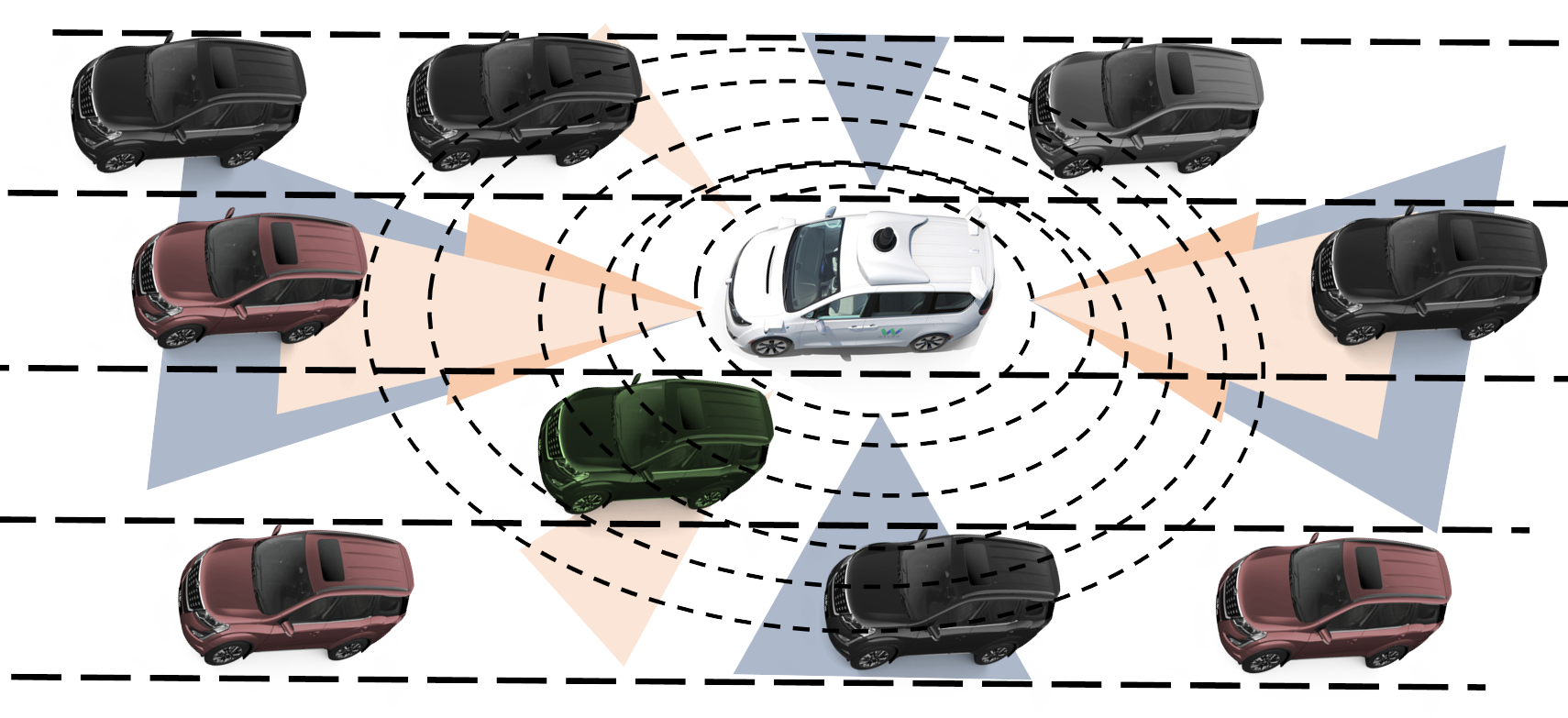
Fig. 1.: Waymo AV and its ambient environment

The dataset comprises two main subsets: perception and motion dataset. This study focuses exclusively on the motion dataset. This subset includes various dynamic and static features, such as the GPS location of the vehicle, its heading direction, speed, acceleration, steering angle, and volume, among other relevant information. A detailed summary of the raw data features are listed in Table 1. The data are captured with a high temporal resolution, having a sampling rate of 0.01 seconds. This fine-grained sampling allows for precise tracking of vehicle dynamics. Each data segment covers a duration of 20 seconds, resulting in a total of 200 frames per segment. This high-frequency sampling and comprehensive feature set enable detailed vehicle motion and behavior analysis over short intervals. The dataset’s distinguishable appearance and extensive feature set allow surrounding HDV to recognize and interact with HDV effectively. This interaction is crucial for studying the interaction patterns and safety aspects of CAVs and HDVs in mixed-traffic environments.

Table 1: Features in available Waymo AV open dataset

Name	Description	Unit
id	Unique ID for each data point
segment id	Unique segment ID for each data point
frame label	Unique Frame ID for each data point
time of day	Day or night
location	Three specific locations: Px, SF, and LA
weather	Sunny, cloudy or dark
laser veh count	Total vehicle count number of each frame
obj type	Vehicle, pedestrian or cyclist
obj id	Unique ID for each object
global time stamp	Global time stamp
global center x	Object global North-South position
global center y	Object global East-West position
global center z	Object global z coordinates
length	Object length	$m$
width	Object width	$m$
height	Object height	$m$
heading	Direction of the object at the instant the data point was captured	$rad$
speed x	Speed of the vehicle along x axis at the instant the data point was captured	$m/s$
speed y	Speed of the vehicle along y axis at the instant the data point was captured	$m/s$
acce x	Acceleration of the vehicle along x-axis at the instant the data point was captured	$m/s^{2}$
accel y	Acceleration of the vehicle along y axis at the instant the data point was captured	$m/s^{2}$
angular speed	Steering angle of the ego vehicle at the instant the data point was captured	$rad$

3.2 2D high-fidelity near-miss risk indicator

SSMs are commonly used to examine near-miss, their effectiveness is limited in real-world scenarios due to their focus on one-dimensional (1D) or longitudinal movement risk scenarios. Traffic interactions (HDV-HDV), especially during maneuvers like merging, lateral movement, and overtaking, require consideration of both the longitudinal and lateral dimensions. While some studies have addressed both dimensions, there are concerns about the accuracy and objectivity of using existing SSMs to characterize various conflicts (see Fig. 3.2). This highlights the need for a versatile, high-fidelity analytical framework to portray complex traffic potential collisions accurately.

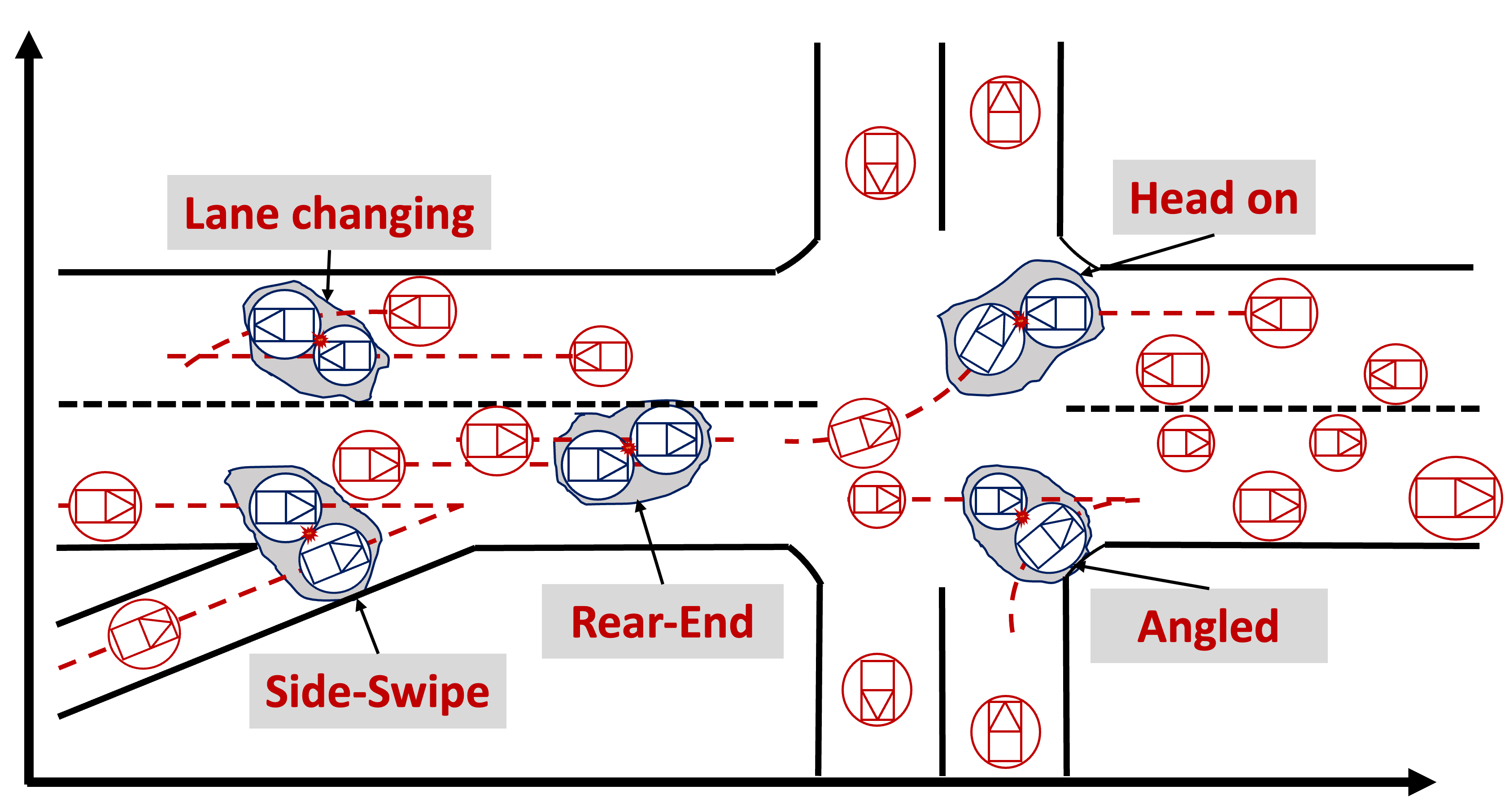
Fig. 2.: Representation of different types of collisions

To address this issue, a 2D high-fidelity TTC derived by Li et al. (2024), which determines potential collisions based on both longitudinal and steering movements of vehicles, is adopted. Assumptions regarding acceleration and steering angle invariance are made each time the TTC is calculated. Under this assumption, the future trajectory of a vehicle is estimated using a state-space model. For a deeper understanding, readers are directed to (Li et al., 2024). To extend the proposed framework beyond 1D, Li et al. (2024) employ a 2D kinematic bicycle model to describe vehicle movements in Cartesian coordinates. This model accounts for the vehicle’s motion in both the x and y directions, providing a comprehensive representation of its dynamics for future state estimation using Eqs. (1)-(4). The model designate the state vector $\chi(t)=[x(t),y(t),\theta(t),v(t)]^{T}$ and the control input vector $u(t)=[\delta(t),a(t)]^{T}$.

$${x}=v\text{~{}cos}(\theta)$$ (1)

$${y}=v\text{~{}sin}(\theta)$$ (2)

$${\theta}=\frac{v\text{~{}tan}(\delta)}{L}$$ (3)

$${v}=a$$ (4)

Here, $(x,y)$ represent the Cartesian coordinates of the vehicle’s center of gravity (C.G.), $\theta$ is the vehicle heading angle, $\delta$ are the steering angles, $L$ is the vehicle’s wheelbase, and $v$ and $a$ are the velocity and acceleration, respectively.

A mathematical condition to represent collisions was proposed by Li et al.(2024), as shown in Eq. (5). The equation calculates the euclidean distance between the centers of the bounding circles of two conflicting vehicles at coordinates $(x_{i},y_{i})$ and $(x_{j},y_{j})$. Setting the distance equal to the sum of their radii, $r_{i}+r_{j}$, implies that vehicles are deemed to collide with each other. Geometrically, this implies that the two bounding circles are tangential to each other (Fig:3.2), representing an imminent collision.

$$g(\chi_{i}(t_{c}),\chi_{j}(t_{c}))$$

$$= (x_{i,t_{c}}-x_{j,t_{c}})^{2}+(y_{i,t_{c}}+y_{j,t_{c}})^{2}-(r_{i}+r_{j})^{2}$$

$$= \biggl{(}-\frac{1}{12}\left(a_{i,0}v_{i,0}\sin(\theta_{i,0})\frac{\tan(\delta_{i,0})}{L_{i}}-a_{j,0}v_{j,0}\sin(\theta_{j,0})\frac{\tan(\delta_{j,0})}{L_{j}}\right)t_{c}^{3}+\frac{1}{2}\biggl{(}a_{i,0}\cos(\theta_{i,0})-v_{i,0}^{2}\sin(\theta_{i,0})\frac{\tan(\delta_{i,0})}{L_{i}}$$

$$-a_{j,0}\cos(\theta_{j,0})+v_{j,0}^{2}\sin(\theta_{j,0})\frac{\tan(\delta_{j,0})}{L_{j}}\biggr{)}t_{c}^{2}+\left(v_{i,0}\cos(\theta_{i,0})-v_{j,0}\cos(\theta_{j,0})\right)t_{c}+(x_{i,0}-x_{j,0})\biggr{)}^{2}$$

$$+\biggl{(}\frac{1}{12}\biggl{(}a_{i,0}v_{i,0}\cos(\theta_{i,0})\frac{\tan(\delta_{i,0})}{L_{i}}-a_{j,0}v_{j,0}\cos(\theta_{j,0})\frac{\tan(\delta_{j,0})}{L_{j}}\biggr{)}t_{c}^{3}+\frac{1}{2}\biggl{(}a_{i,0}\sin(\theta_{i,0})+v_{i,0}^{2}\cos(\theta_{i,0})\frac{\tan(\delta_{i,0})}{L_{i}}$$

$$-a_{j,0}\sin(\theta_{j,0})-v_{j,0}^{2}\cos(\theta_{j,0})\frac{\tan(\delta_{j,0})}{L_{j}}\biggr{)}t_{c}^{2}+\left(v_{i,0}\sin(\theta_{i,0})-v_{j,0}\sin(\theta_{j,0})\right)t_{c}+(y_{i,0}-y_{j,0})\biggr{)}^{2}-(r_{i}+r_{j})^{2}$$ (5)

Here $t_{c}$ is the time after which two vehicles would collide if they move with the same steering angle and acceleration, where subscript $i$ and $j$ denote the indices corresponding to individual vehicles, $r$ is the radius of the vehicle from the center.

By setting $g(x_{i}(t_{c}),x_{j}(t_{c}))=0$ and solving for feasible $t_{c}$, a novel 2D TTC is obtained, as detailed in Eq. (6) and Fig. (3.2).

$$\text{TTC}_{ij}=\begin{cases}t_{c},&\text{if }g(x_{i}(t_{c}),x_{j}(t_{c}))=0\text{ and }t_{c}\geq 0\\ \infty,&\text{otherwise}\end{cases}$$ (6)

AV sensor data contains granular information for vehicles $i$ and $j$ in each frame of $z$. To identify the minimum TTC for any given pair of conflicting vehicles, we calculate the TTC between vehicle $i$ and vehicle $j$ at frame $z$ denoted as $\text{TTC}_{ij}(z)$. The minimum TTC for any vehicle pair across all frames can be determined using the following equation.

$$\text{X}=\text{TTC}_{\text{min}}(i,j)=\min_{z\in\{1,2,\ldots,n\}}\{\text{TTC}_{ij}(z)\}$$ (7)

This equation defines X as the minimum TTC value observed between vehicles $i$ and $j$ over n frames.

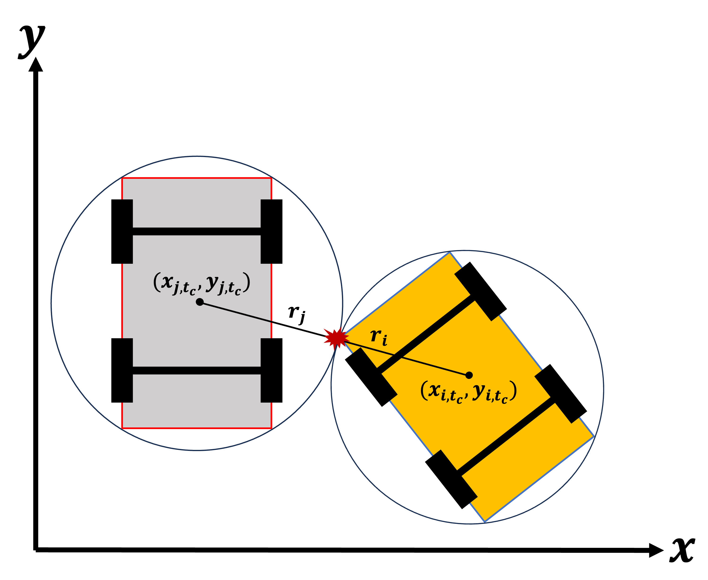
Fig. 3.: Description of Eq.5

3.3 Univariate generalized extreme value distribution

Extreme Value Theory (EVT) is applied to derive near-miss or traffic conflict risk from surrogate safety measures (SSM) due to its effectiveness in identifying a strong correlation between observed near-miss risks and actual crashes. This risk was quantified using EVT, which enables precise modeling of extreme traffic conflicts, also known as tail events. In general, EVT employs two main approaches for fitting the tail distribution of these extreme conflicts: Block Maxima/Minima (BM) and Peaks Over Threshold (POT). Several studies reveal that the POT method often yields more efficient estimates since it accounts for all extreme observations, whereas the BM method might overlook some significant observations within the same block (Ferreira and De Haan, 2015). For instance, Zheng et al.(2014) found that the POT method outperformed the BM method in terms of data utilization, estimate accuracy, and reliability. Similarly, Orsini et al. (2019) also reported promising results for both BM and POT methods, particularly when using the 1/TTC approach. However, Bucher et al. (2021) argued that the choice of method should be guided by the statistical interest, with POT being preferable for quantile estimation and BM for return level estimation. Ferreira (2015) provided conditions under which the BM method can be justified, suggesting that it is efficient under practical conditions. Nonetheless, recent research indicates that the convergence rates of these methods can vary based on the underlying data process, with no definitive superior approach. BM models generally exhibit smaller variance but more significant bias than POT models.

The BM approach is frequently chosen for real-time applications since it considers equal intervals of the observation period, making metrics like crash risk suited for immediate scenarios and time-sensitive (Songchitruksa and Tarko, 2006). Conversely, the POT approach assesses safety levels based on instances that exceed a certain severity threshold, making it better for aggregated safety estimates. Consequently, this study employs the BM approach due to its practical advantages in real-time crash risk assessment and its efficiency under the given conditions.

The BM approach, a fundamental method for developing generalized extreme value distribution (GEV), involves dividing observations into fixed time blocks and treating the maximum or minimum value within each block as an extreme event (Coles et al., 2001). Assuming a common distribution for a series of independent random variables $X_{1},X_{2},\ldots,X_{n}$, within a block, the maximum values such as $M_{n}=\max\{-X_{1},-X_{2},\ldots,-X_{n}\}$ of $n$ observations, where X are derived from Eqn. 7 and used negative values for block minima distribution. A GEV distribution will be converged if normalized maximum values $M_{n}^{*}=\frac{M_{n}-a_{n}}{b_{n}}$.

In the univariate case, if there are sequences of constants $a_{n}>0$ and $b_{n}$ such that:

$$\Pr\left(\frac{M_{n}-a_{n}}{b_{n}}\leq X\right)\to F(X)\quad\text{as}\quad n\to\infty$$

where $F$ is a non-degenerate distribution function that belongs to the Gumbel, Fréchet, or Weibull distribution families, which are all part of the GEV distribution (Coles et al., 2001), shown in Eqn (8).

$$f(X;\mu,\sigma,\xi)=\exp\left\{-\left[1+\xi\left(\frac{X-\mu}{\sigma}\right)\right]^{-1/\xi}\right\}$$ (8)

where $[1+\xi\left(\frac{X-\mu}{\sigma}\right)>0]$, $-\infty<\mu<\infty$, $\sigma>0$, $-\infty<\xi<\infty$, $\xi>0$ for Fréchet and $\xi<0$ for Weibull, $\xi=0$ for Gumbel distribution of GEV

3.3.1 Hierarchical Bayesian structure random parameter (HBSRP) model

This study employs a hierarchical Bayesian structure with a random parameter (HBSRP) model that offers greater flexibility than fixed parameter models by accounting for unobserved heterogeneity among different sites. By employing a multi-site strategy, the HBSRP model improves effectiveness using precise safety performance metrics from stable regions to inform more unstable ones. The data level, process level, and prior level make up the three layers that make up the Bayesian structure of the model. Extreme TTC for each block is modeled at the data level using a GEV distribution. The process level incorporates a Gaussian Process (GP) latent variable to capture spatial or temporal correlations and unobserved heterogeneity. The prior level involves selecting appropriate prior distributions, including their means and variances, to characterize each parameter and address uncertainties effectively.

By applying Bayes’ theorem, the parameters $\Omega$ for the univariate extreme value model with a three-layer hierarchical structure given the data $X$, are inferred through the posterior distribution as formulated in Eqn (9):

$$q(\Omega\mid X)\propto q_{\text{data}}(X\mid\Omega_{1})q_{\text{process}}(\Omega_{1}\mid\Omega_{2})q_{\text{prior}}(\Omega_{2})$$ (9)

Here, $q(\Omega\mid X)$ represents the posterior distribution of the parameters $\Omega$ given the observed data $X$. This posterior distribution is obtained by combining the likelihood of the data layer $q_{\text{data}}(X\mid\Omega_{1})$, with the process layer $q_{\text{process}}(\Omega_{1}\mid\Omega_{2})$ and prior layer $q_{\text{prior}}(\Omega_{2})$. The density functions of $q_{\text{data}},q_{\text{process}},q_{\text{prior}}$ are given below

The HBSRP model is formulated by denoting $k_{n}$ as the number of extreme traffic conflicts observed in the $n$-th block ($n=1,2,3,\ldots,k_{n}$) and $X_{nm}$ as the traffic conflict of the $n$-th block within the $m$-th site ($m=1,2,3,\ldots,i_{m}$). The magnitudes of the $k_{n}$ events occurring within a block are assumed to be realizations of independent and identically distributed random variables $X_{nm}$ with a common parametric cumulative distribution function $f$.

Due to the positive property of the scale parameter, the GEV distribution $(\mu,\sigma,\xi)$ is reparametrized as GEV $(\mu,\vartheta,\xi)$ where $(\vartheta=\log\sigma)$. Therefore, letting $\mu_{m},\vartheta_{m},\xi_{m}$ denote the parameters at the site $m$, the expression for the joint probability density function (pdf) of the reparameterized GEV distribution for all events is given by Eqn (10):

$$q_{\text{data}}(X\mid\Omega_{1})=\prod_{m=1}^{i}\prod_{n=1}^{k_{m}}\left(\frac{1}{\exp(\vartheta_{m})}\right)\exp\left\{-\left[1+\xi_{m}\left(\frac{X_{nm}-\mu_{m}}{\exp(\vartheta_{m})}\right)\right]^{-1/\xi_{m}}\right\}\left[1+\xi_{m}\left(\frac{X_{nm}-\mu_{m}}{\exp(\vartheta_{m})}\right)\right]^{-1-1/\xi_{m}}$$ (10)

The cumulative distribution function for $X_{nm}$ given the parameters $\mu_{m},\vartheta_{m},\xi_{m}$ is given by Eqn (11):

$$f(X_{nm}<X\mid\mu_{m},\sigma_{m},\xi_{m})=\exp\left\{-\left[1+\xi_{m}\left(\frac{X-\mu_{m}}{\exp(\vartheta_{m})}\right)\right]^{-1/\xi_{m}}\right\}$$ (11)

This study utilizes a latent Gaussian process to model extremes, specifically linking data layer parameters to covariates through identity link functions. A significant challenge in this approach is accurately estimating the shape parameter $\xi$ of the GEV distribution. As it is unrealistic to construct a smooth function of covariates for $\xi$, it is generally treated as unknown and not influenced by covariates (Coles et al., 2001; Cooley et al., 2006). The model introduces random coefficients to address unobserved heterogeneity among observation sites, as shown in Eqn (12). Random intercept coefficients capture site-specific heterogeneity unrelated to explanatory variables, while random coefficients account for the variation in covariate effects across different sites. This approach allows for a more thorough representation of unobserved heterogeneity, improving traffic safety analysis’s accuracy and reliability by incorporating consistent site-specific factors and variable covariate impacts across sites.

$$\mu_{m} =\alpha_{\mu_{0m}}+\alpha_{\mu_{m}}Y$$ (12)

$$\vartheta_{m} =\alpha_{\vartheta_{0m}}+\alpha_{\vartheta_{m}}Y$$

$$\xi_{m} =\alpha_{\xi_{0m}}$$

Where, $\alpha_{\mu_{0m}},\alpha_{\mu_{m}},\alpha_{\vartheta_{0m}},\alpha_{\vartheta_{m}},\alpha_{\xi_{0m}}$ are random coefficients and $Y$ is an explanatory variable. With these parameters, the process layer works according to Eqn (13):

$$q_{\text{process}}(\Omega_{1}\mid\Omega_{2})=\frac{1}{\sqrt{2\pi\tau_{\mu}^{2}}}\exp\left\{-\frac{1}{2\tau_{\mu}^{2}}(\mu-\mu_{m})^{2}\right\}\times\frac{1}{\sqrt{2\pi\tau_{\vartheta}^{2}}}\exp\left\{-\frac{1}{2\tau_{\vartheta}^{2}}(\vartheta-\vartheta_{m})^{2}\right\}\times\frac{1}{\sqrt{2\pi\tau_{\xi}^{2}}}\exp\left\{-\frac{1}{2\tau_{\xi}^{2}}(\xi-\xi_{m})^{2}\right\}$$ (13)

In Bayesian analysis, it is crucial to identify appropriate prior distributions. For this study, noninformative priors were selected empirically. The model parameters $\alpha_{\mu_{0m}},\alpha_{\mu_{m}},\alpha_{\vartheta_{0m}},\alpha_{\vartheta_{m}},\alpha_{\xi_{0m}}$ are assigned normal prior distributions, specifically $N(\delta_{\mu},\delta_{\sigma})$. The mean $\delta_{\mu}$ of these distributions is itself normally distributed $\delta_{\mu}\sim N(0,0.00001)$. The variance $\delta_{\sigma}$ follows an inverse gamma distribution $\delta_{\sigma}\sim\text{IG}(0.001,0.001)$. The shape parameter $\xi$ of the GEV distribution is typically uniformly distributed between -1 and 1; according to Fu et al. (2020), the criterion for selecting these prior distributions is the successful convergence of the model, and the prior works as Equation (14).

$$q_{\text{prior}}(\Omega_{2})=q_{\alpha_{\mu_{0}}}(\alpha_{\mu_{0}})\times q_{\alpha_{\mu_{m}}}(\alpha_{m})\times q_{\alpha_{\vartheta_{0}}}(\alpha_{\vartheta_{0}})\times q_{\alpha_{\vartheta_{m}}}(\alpha_{m})\times q_{\alpha_{\xi_{0}}}(\alpha_{\xi_{0}})$$ (14)

3.3.2 Model choice

When developing the HBSRP model, which links the location and scale parameters of the GEV distribution to several covariates, numerous model choices are available. The Deviance Information Criterion (DIC) is widely used within the Bayesian framework for model selection. The principle of DIC is parsimony, aiming to find the simplest model that explains the most variation in the data. The DIC is calculated as Eqn (15):

$$\text{DIC}=\bar{D}+p_{D}$$ (15)

where $\bar{D}$ is the posterior mean deviance, indicating model fit, and $p_{D}$ is the adequate number of parameters. Generally, a model with a lower DIC is preferred. A difference greater than 10 in DIC values between models strongly favors the model with the lower DIC. Differences between 5 and 10 are considered substantial, while differences less than 5 suggest that the models are competitive.

3.3.3 Crash estimation

The Risk of Crash (RC) index is a probabilistic measure derived from the GEV distribution, used to quantify the likelihood of a crash based on TTC data. In this context, a crash is defined as having a TTC equal to zero. The RC index represents the probability that the maximum negated TTC in a given block exceeds zero. The likelihood for block $n$ is given by Eqn (16):

$$\text{RC}_{n}=\Pr(X_{n}\geq 0)=\begin{cases}1-\exp\left\{-\left[1-\xi_{n}\left(\frac{\mu_{n}}{\exp(\vartheta_{n})}\right)\right]^{-1/\xi_{n}}\right\},&\xi_{n}\neq 0\\ 1-\exp\left\{-\exp\left(\frac{\mu_{n}}{\exp(\vartheta_{n})}\right)\right\},&\xi_{n}=0\end{cases}$$ (16)

In this equation, $\xi_{n}$, $\vartheta_{n}$, and $\mu_{n}$ are the GEV distribution’s shape, scale, and location parameters, respectively. The value of $\text{RC}_{n}$ ranges from 0 to 1, where 0 indicates no crash risk and values closer to 1 indicate higher crash risk. This index provides a quantitative measure of crash probability, enabling researchers and engineers to identify high-risk areas and implement safety interventions accordingly.

The estimated crash risk can be translated to extended periods beyond the observation period, such as annually. To calculate the crash frequency for both the observation period and yearly, use Eqn (17):

$$\text{CF}=\sum_{n=1}^{k}\text{RC}_{n}$$ (17)

$$\text{CF}_{\text{year}}=\frac{T}{t}\times\text{CF}$$ (18)

where CF is defined as crash frequency, $t$ is the number of block maxima used in the observation period, and $T$ is the total block maxima data yearly included in the model.

4 Analysis and results

4.1 Data preparation

The dataset for this study was meticulously extracted from the Waymo fleet data (described in section 3.1), currently operating in various urban networks across cities such as San Francisco, Phoenix, and Los Angeles. Two segments were chronologically selected ( see Fig. 4.1) for each of these cities based on specific criteria designed to capture diverse and complex traffic scenarios as depicted in Fig. 3.2. The selected segments considered high traffic movement, presence of lane-changing vehicles, pedestrians, cyclists, multiple midblock sections, and intersections to represent diverse HDV behaviors and capture more complex 2D HDV movements.

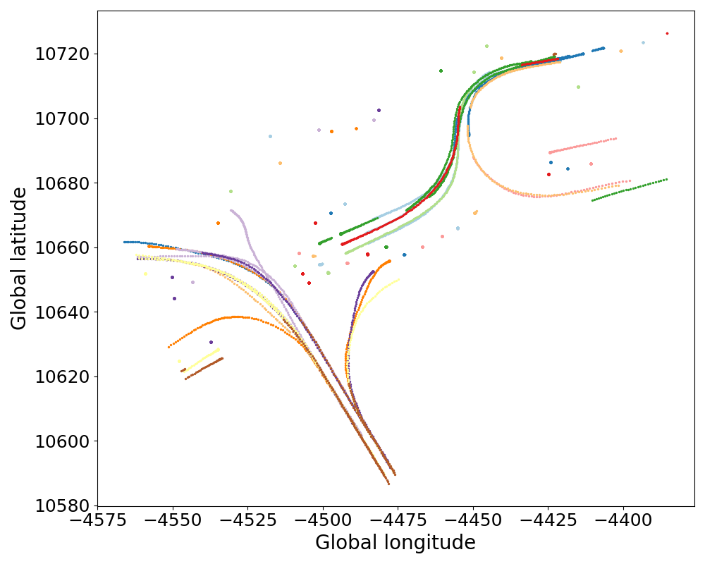
(a) Site-1

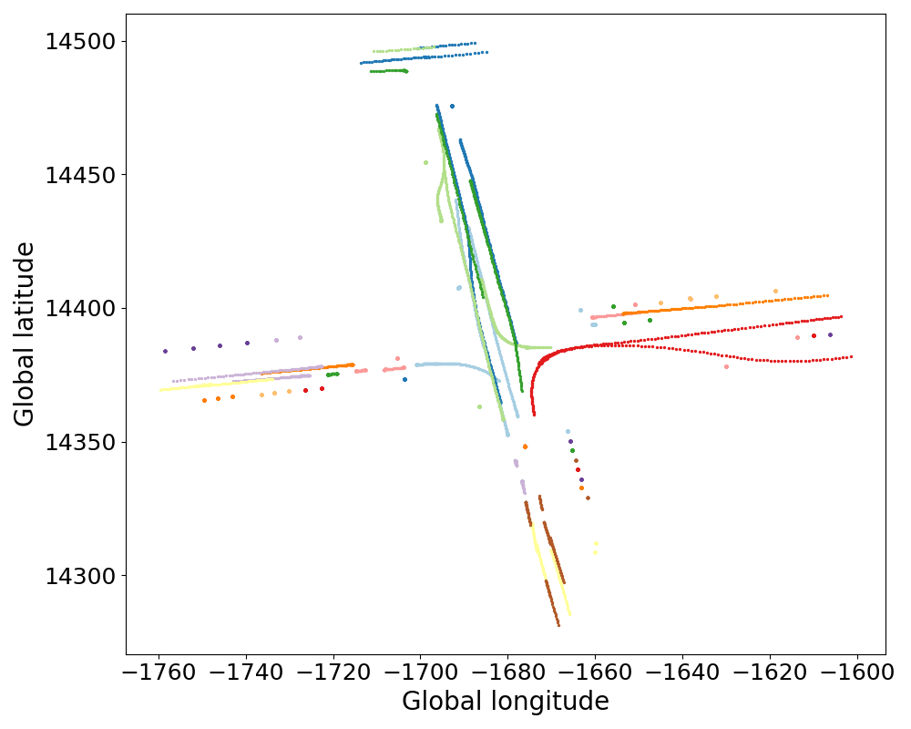
(b) Site-2

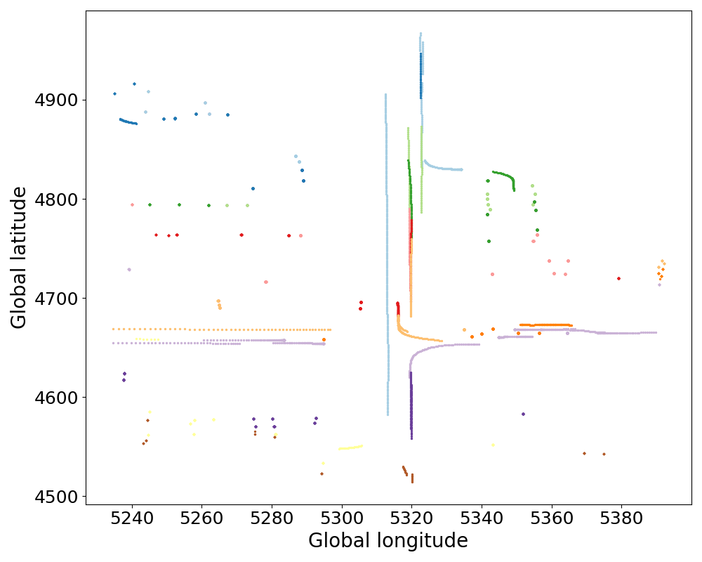
(c) Site-3

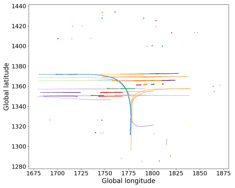
(d) Site-4

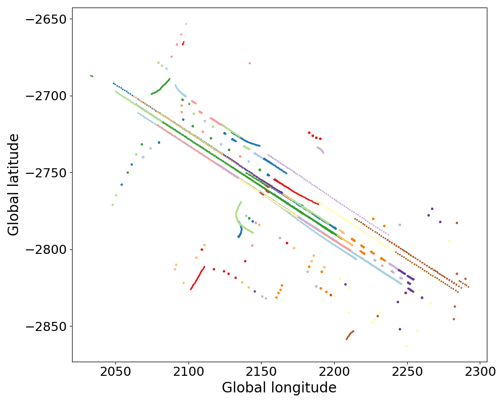
(e) Site-5

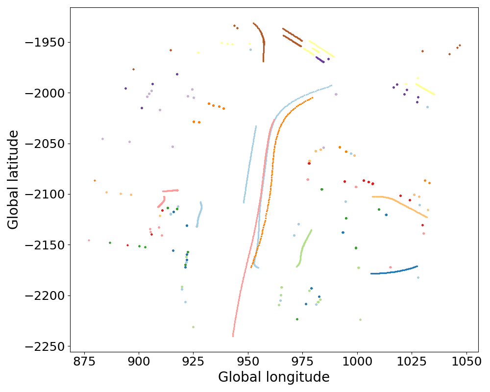
(f) Site-6

Fig. 4.: The study locations: San Francisco (1&2), Phonix (3&4), Los Angeles (5&6)

The data preparation for this analysis involved several key steps. This initial extraction aimed to gather comprehensive data from the most relevant ambient environment. Other road users, such as pedestrians and cyclists, were excluded from the dataset to focus solely on HDV-HDV interactions. This exclusion helped concentrate on the primary area of interest for this study. The extracted data was meticulously cleaned to remove any anomalies, duplicates, or irrelevant information. This step ensured the dataset’s integrity and accuracy, providing a reliable foundation for further analysis. The cleaned data was segmented chronologically for each city, and all detected objects’ information and other relevant information, as listed in Table 1. This step ensured that the selected segments met the high-traffic movement and complex interaction criteria, focusing on relevant HDV behaviors. These features included vehicle speed, acceleration, steering angles, heading, and other information. This selection was crucial to capturing the essential dynamics of HDV movements. The dataset includes real-time local positions of all detected HDVs identified by the LiDAR system of the Waymo ego vehicle at each time step. To utilize this information effectively, it is necessary to transform the HDVs’ local headings into global headings. While the Waymo vehicle’s heading ($\alpha$) is already in the global coordinate system, the HDVs’ headings ($\alpha^{\prime}$) are measured in the local coordinate system relative to the ego vehicle. Therefore, to convert these local headings into the global coordinate system, we add the Waymo vehicle’s global heading to each HDV’s local heading. This transformation process, illustrated in Fig. 4.1(a), is expressed mathematically as:

(a) Heading

(b) Speed

(c) Acceleration

Fig. 5.: Transformation to the global reference

$$\theta =\alpha+\alpha^{\prime}$$ (19)

where $\theta$ represents the global heading of an HDV. This step is crucial for ensuring that the orientation of each HDV is accurately represented in the global context, which is essential for task trajectory calculation. Similarly, speed, acceleration, and steering angle data were transformed into the global reference frame for all vehicles, as shown in Fig. 4.1(b)&(c). The transformations are given by:

$$v =v_{x}\cos\theta+v_{y}\cos\left(\frac{\pi}{2}-\theta\right)$$ (20)

$$a =a_{x}\cos\theta+a_{y}\cos\left(\frac{\pi}{2}-\theta\right)$$ (21)

$$\delta =\tan^{-1}\left(\frac{\dot{\theta}L}{v}\right)$$ (22)

where $v$ is the global speed, $v_{x}$ and $v_{y}$ are the speed components in the local coordinate system. Where $a$ is the global acceleration, $a_{x}$ and $a_{y}$ are the acceleration components in the local coordinate system. Where $\delta$ is the global steering angle, $\dot{\theta}$ is the rate of change of the heading angle in each frame, and $L$ is the vehicle’s wheelbase. These transformations are essential for ensuring that the speed, acceleration, heading, and steering angle data of HDVs are accurately represented in the global coordinate system. After transforming these parameters into the global reference frame, they are applied in the HDV-HDV interaction function in Eq. 5. This transformation ensured consistency and comparability across the dataset.

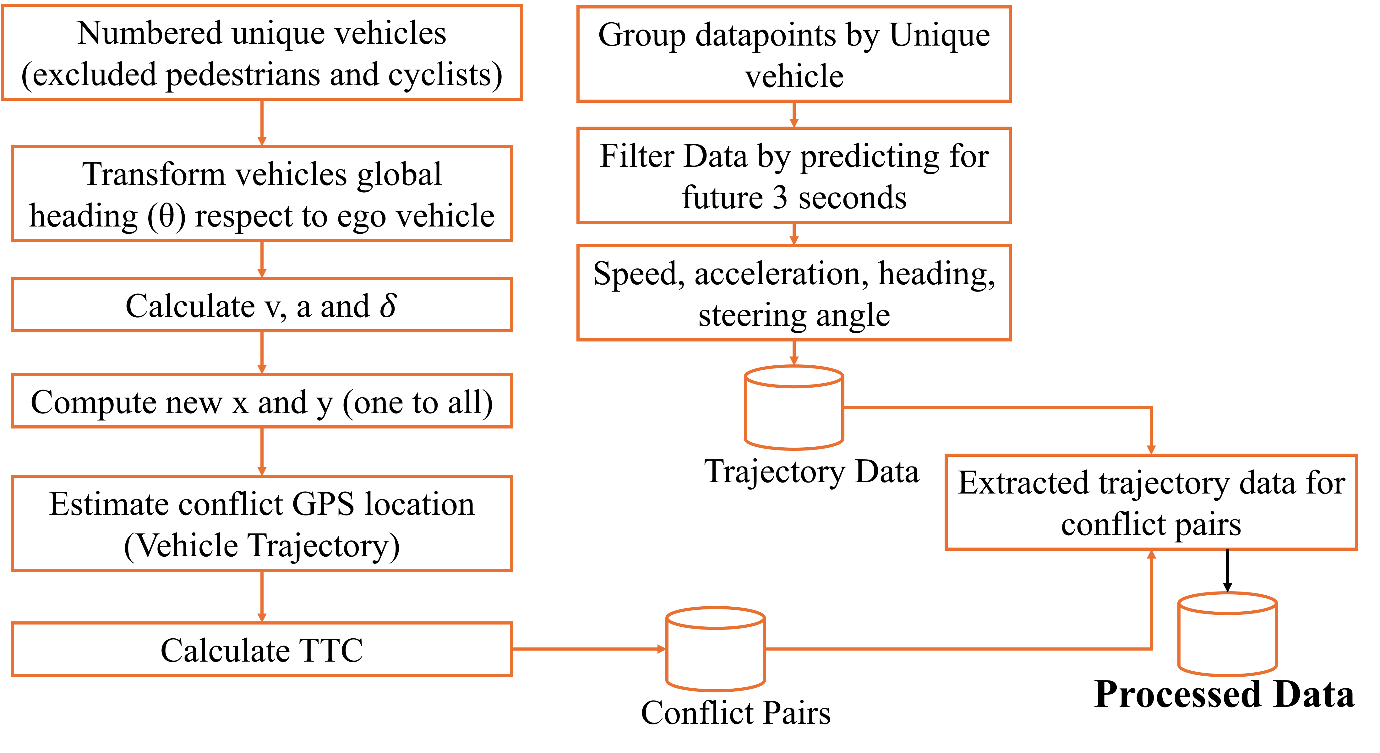
Fig. 6.: Data processing pipeline for calculating TTC from conflicting pairs

The data processing pipeline, illustrated in Fig. 4.1, employs two separate pipelines: one for identifying conflict pairs and another for processing trajectory data. This dual-pipeline approach facilitated the efficient handling and analysis of the complex dataset. By calculating 2D-based TTC for all vehicles over 200 frames, within a boundary of 0.1 to 3 seconds using Eqns (5) and (6), the method identifies all conflicting pairs frame by frame, as depicted in Fig. 4.1.

Fig. 4.1 visually represents a subset of the sequential TTC calculation process for unique conflicting vehicle pairs over 200 frames. Each sub-figure, shown from Frame-1 to Frame-6, captures the dynamic interactions between two vehicles moving closer to a potential collision. Initially, Frame-1 calculates the TTC using Eqns (5) and (6) based on their starting positions, velocities, accelerations, steering angles, and headings. As the frames progress, the positions and distances between the vehicles are updated based on their trajectories and the recalculated TTC values. Frame-2 through Frame-6 depict intermediate stages where the TTC values decrease as the vehicles approach each other, highlighting the increased risk of collision. For instance, in Frame 6, vehicles 21 and 46 are shown in close proximity, with a minimal TTC indicating a high collision risk, resulting in a TTC of 1.647s for this conflicting pair. So, calculated TTC illustrates the point of imminent collision with minimal TTC value if no evasive actions are taken. This detailed series of frames demonstrates the real-time calculation of TTC using high-resolution Waymo sensor data, emphasizing the critical moments leading up to a potential crash.

(a) Frame-1

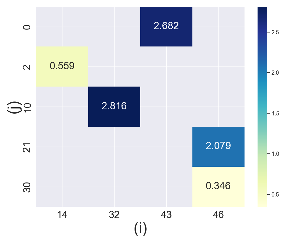
(b) Frame-2

(c) Frame-3

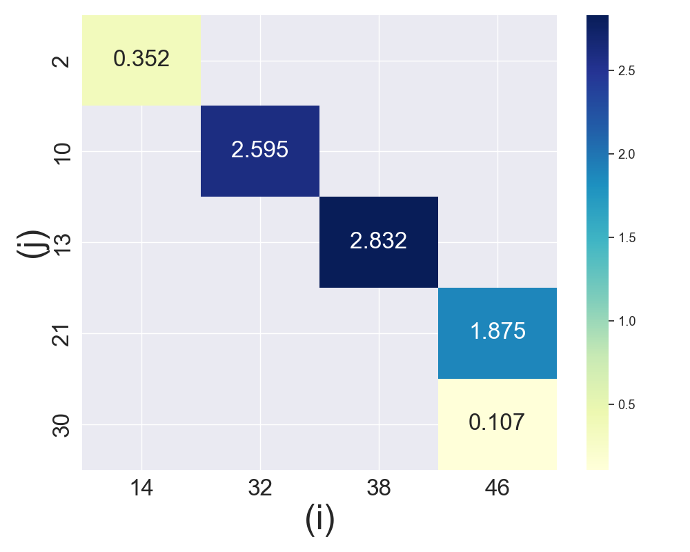
(d) Frame-4

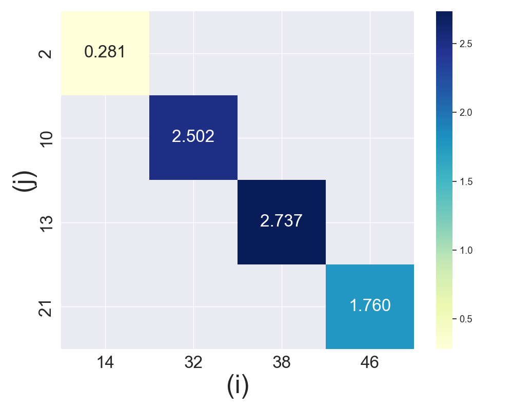
(e) Frame-5

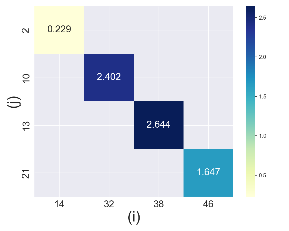
(f) Frame-6

Fig. 7.: TTC calculation of conflicting pairs

Fig. 4.1 presents a detailed analysis of how various exogenous variables impact the TTC. The figure comprises several subplots, each focusing on different parameters. The first subplot Fig. 4.1(a) illustrates the effect of the volume, speed, and acceleration of conflicting vehicles on TTC. It shows no definite trend among TTC, speeds, acceleration, and deceleration. However, it indicates that high volume results in higher conflict crash risk, thereby increasing the risk of collision as vehicles approach each other more rapidly. Fig. 4.1(b) demonstrates the influence of vehicle length, speed, and acceleration on TTC. It suggests that smaller vehicles increase collision risk by reducing TTC values, emphasizing the critical role of vehicle length in potential crash scenarios. Fig. 4.1(c) explores the impact of steering angle changes, speed, and acceleration on TTC. It reveals that TTC values decrease when a vehicle is moving toward another vehicle, indicating increased collision risk. These insights underscore the importance of vehicle dynamics, particularly speed and acceleration, in determining collision risks. They highlight the need for further investigation into the relationship between these variables to enhance our understanding of potential crash scenarios.

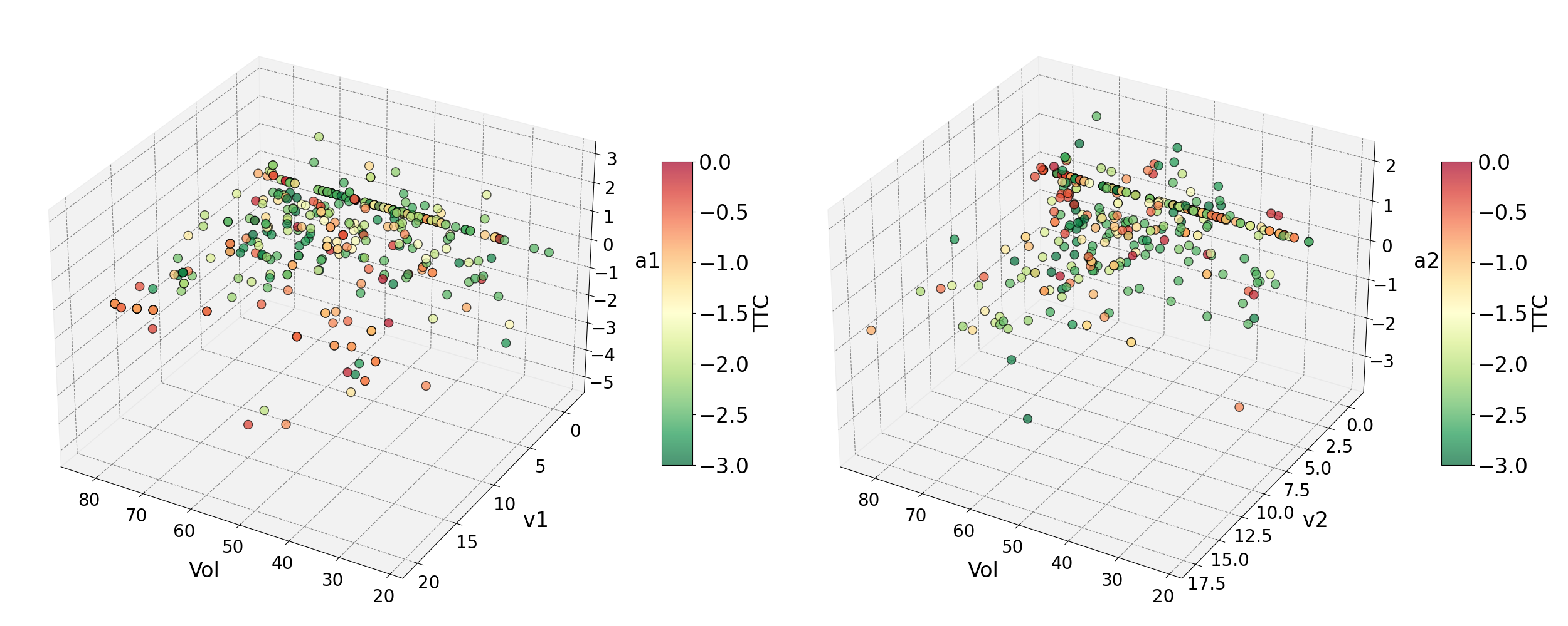
(a) Relationship among volume, speed, acceleration and TTC

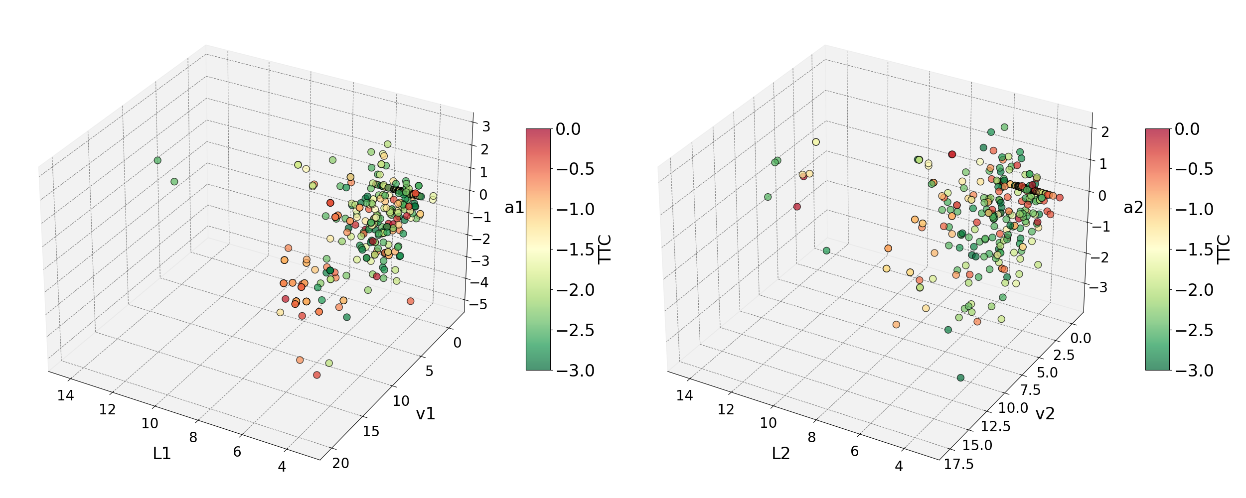
(b) Relationship among length, speed, acceleration and TTC

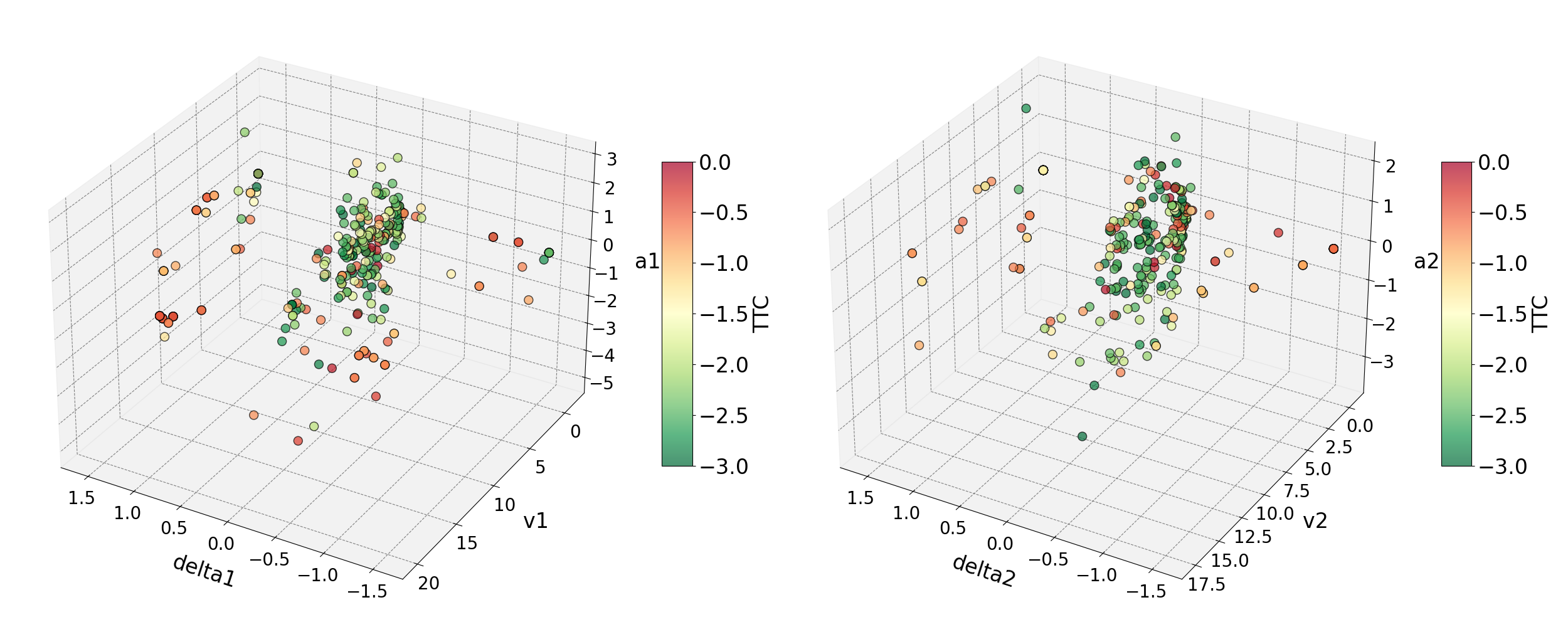
(c) Relationship among steering angle, speed, acceleration and TTC

Fig. 8.: Effect of exogenous variables on TTC

As described in 3.1, to derive 2D-based TTC to crash risk using GEV distribution requires a suitable sample size for fitting curves. Therefore, block segmentation is crucial to selecting an appropriate block size. The block maxima/minima approach, as described by Songchitruksa and Tarko (2006), uses a time-based sampling scheme where observations are divided into fixed time intervals, and the maxima (or minima) from each block are treated as extremes. The literature does not provide a consensus on the optimal block size, with studies using block sizes ranging from 2-3 minutes to 20 minutes. Recent studies by Fu et al. (2022b; 2022a) and Zheng and Sayed (2019) have used a 20-minute block size and compared it with other block sizes based on local goodness-of-fit (GOF) measures such as Bayesian Information Criterion (BIC). While local GOF provides insights into model fit, it is also essential to evaluate the effects of block size using global measures like mean crash estimates and confidence intervals of crash estimates.

The methodology for identifying extreme traffic events from sensor data differs from video data, favoring shorter intervals for detailed analysis. In this study, each conflicting pair is treated as a block, and the minima of TTC selected for each pair are considered extreme traffic events, as shown in Eqn. 7, as used in a simulator-based study by Ali et al. (2022). Selecting the minima of each frame could lead to biased parameter estimates due to the granular nature of each frame having the same conflicting pairs of information. To avoid this, the study uses the conflicting pair as a block. This approach, driven by the availability of micro-level data, mitigates errors from time-varying driver behaviors (Mannering, 2018). Few studies argue that the poor performance of estimated GEV models is often attributed to sample size, but this is debatable. Although more data over longer periods is generally preferred, extended data collection can also introduce errors from temporal shifts in driver behavior.

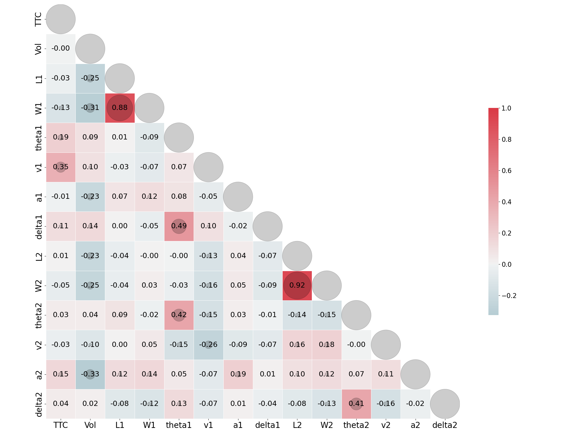
Fig. 9.: Correlation matrix of exogenous variables

Fig. 4.1 provides a comprehensive correlation matrix illustrating the relationships between various exogenous variables of the used dataset in this study. The matrix includes key variables such as traffic volume (Vol), vehicle lengths (L1, L2), vehicle widths (W1, W2), vehicle speeds (v1, v2), vehicle accelerations (a1, a2), and steering angles (theta1, theta2). Each cell contains a correlation coefficient value ranging from -1 to 1, indicating the strength and direction of the relationship between two variables. Significant correlations are evident in the matrix, such as the strong positive correlation between vehicle widths and length, suggesting that large vehicles tend to be consistently wider across different measurements. Another notable correlation is the strong positive relationship between vehicle heading and steering angle. The matrix also shows moderate negative correlations between traffic volume, vehicle speed, and acceleration, implying that higher traffic volumes are associated with decreased vehicle speeds and acceleration. These insights are crucial for understanding the dynamics of traffic conflicts and the interactions between vehicles and traffic characteristics. For instance, the relationships between speed, volume, and dimensions can help identify potential risk factors and improve the accuracy of traffic conflict predictions.

For each location, unique conflicting pairs’ minimum negated TTC_min were determined for each block, representing the BM. These values, along with traffic volume, conflicting pairs’ average speed, and average acceleration, were then used as covariates in the GEV model. Conflict data, summarized for each site, revealed total conflicts with TTC 3.0 seconds ranging from 45 to 108 across six sites (see Table. 2). This table provides a detailed summary of statistics and vehicle dynamics variation across six distinct sites, highlighting key metrics such as block minimum TTC, traffic volume, and the vehicles’ speed and acceleration/deceleration characteristics. Site 5 exhibits the highest frequency of conflict events 108 and a notably high average traffic volume 77, with Vehicle-1 showing a significant speed of 7.78 m/s and deceleration of -0.56 m/s², indicating a potentially high-risk area with frequent traffic interactions and abrupt vehicle maneuvers. Conversely, Site 3, with the lowest frequency of conflict events of 45 and a relatively low traffic volume of 37, displays distinct vehicle dynamics where Vehicle-2 has a high speed of 9.7 m/s but minimal deceleration of -0.17 m/s², suggesting less frequent but more severe interactions. Sites 1 and 2, with moderate conflict frequencies of 58 and 95, respectively, show a balance in vehicle dynamics with moderate speeds and mixed acceleration/deceleration patterns, reflecting typical urban traffic conditions with diverse movement behaviors. Site 4, with a moderate conflict frequency of 61 and balanced vehicle dynamics, indicates a mix of interactions with both vehicles displaying similar acceleration patterns, pointing to synchronized traffic behavior. Site 6, with the lowest traffic volume of 53 and minimal vehicle speeds, suggests a less dynamic but stable traffic environment.

Table 2: Summary statistics of each site

Site	Block minima	TTCmin (s)			Traffic vol/frame	Vehicle-1		Vehicle-2
	(Frequency)	avg	min	max		spd (m/s)	acc/dec (m/s${}^{2}$)	spd (m/s)	acc/dec (m/s${}^{2}$)
1	58	1.96	0.1	3.00	64	3.89	-0.255	2.61	-0.15
2	95	2.18	0.1	3.00	53	2.4	0.06	3.33	-0.09
3	45	1.21	0.15	2.846	37	9.7	-0.17	2.45	0.07
4	61	1.36	0.1	2.92	49	4.9	0.57	4.55	0.66
5	108	1.44	0.1	2.97	77	7.78	-0.56	2.24	-0.48
6	55	1.58	0.3	2.53	53	1.13	-0.03	0.87	0.04

4.2 Model estimation inference

Several hierarchical Bayesian univariate models were developed for six sites across three cities to estimate crash risks from calculated TTC data. Instead of modeling individual sites separately, the GEV distribution was fitted to the data as a network. This approach addresses the issue of sample scarcity by effectively grouping the sites by city. Using the OpenBUGS tool, which facilitated the complex computations required for this analysis, we estimated the posterior distributions of each model parameter through Markov Chain Monte Carlo (MCMC) algorithms. Due to the inherent bias and auto-correlation MCMC samples, we conducted numerous iterations to mitigate these effects. Multiple simulation chains, each beginning with different initial values, were run to ensure robust convergence. Precisely, two chains were executed for 50,000 iterations for each parameter, with the first 20,000 discarded as burn-in. The subsequent 30,000 iterations provided the data for posterior estimates.

To assess convergence, we visually inspect trace plots that display the progression of chains from varied starting points, as well as calculate the Brooks-Gelman-Rubin (BGR) statistic for each parameter (El-Basyouny and Sayed, 2009). The BGR statistic, which stabilized around 1 (less than 1.1), indicates that the models had converged effectively (Gelman and Rubin, 1992).

The DIC values used to evaluate four distinct GEV models in this study are presented in Tables 3, 4, and 5. These models include stationary models with fixed parameters, which assume consistency across all observations, and stationary models with random parameters, allowing for data variability at different sites. The non-stationary model with location and scale parameterized accommodates non-stationary behavior by allowing these parameters to vary over sites. Meanwhile, the non-stationary model with a random location and a scale-parameterized model provides a more dynamic analysis framework. Our evaluation reveals that non-stationary models, particularly those that parameterize location and scale, significantly outperform their stationary counterparts in fitting the data. This superior performance is enhanced by the strategic inclusion of covariates in the model, which captures more nuanced variations and interactions within the data, offering more profound insights into HDV-HDV interactions and improving the model’s GOF. Among the two non-stationary models, the most effective, which featured the lowest DIC value, included random parameters for different sites and covariates in the location and scale parameters. This model was selected for further study due to its robustness and accuracy in crash risk estimation.

Initial exogenous covariates consider the time of day, weather, laser vehicle count, object length, width, height, speed, acceleration, heading, and steering angle. However, due to their statistical insignificance, the final retained model did not include some covariates, such as time of day, weather, object dimensions, heading, and steering angle. The laser vehicle count covariate was also excluded from the final models due to its correlation with vehicle speed and acceleration, which could lead to multicollinearity issues. This approach ensures a more robust and parsimonious model, improving the reliability and accuracy of the crash risk estimates.

Table 3: Model estimation results for sites 1&2 (San Francisco)

Model parameters		Stationary								Non-Stationary
		FP				RP				FP				RP
		Mean	SD	2.5%	97.5%	Mean	SD	2.5%	97.5%	Mean	SD	2.5%	97.5%	Mean	SD	2.5%	97.5%
$\mu$	$\alpha_{\mu_{0}}$	-2.499	0.04	-2.576	-2.418					-2.489	0.037	-2.56	-2.413
	$\alpha_{\mu_{0[1]}}$					-2.485	0.103	-2.667	-2.268					-2.605	0.064	-2.718	-2.467
	$\alpha_{\mu_{0[2]}}$					-2.491	0.039	-2.565	-2.411					-2.472	0.035	-2.538	-2.402
	$\alpha_{\mu_{\text{spd\_veh1}}}$
	$\alpha_{\mu_{\text{spd\_veh2}}}$									-0.047	0.008	-0.0613	-0.0281	-0.028	0.008	-0.044	-0.013
	$\alpha_{\mu_{\text{acc\_veh1}}}$													-0.049	0.024	-0.094	-0.030
	$\alpha_{\mu_{\text{acc\_veh2}}}$
$\vartheta=\log(\sigma)$	$\alpha_{\vartheta_{0}}$	-0.846	0.08	-1.0	-0.688					-0.888	0.0787	-1.04	-0.732
	$\alpha_{\vartheta_{0[1]}}$					-0.566	0.166	-0.901	–0.254					-0.795	0.158	-1.098	-0.478
	$\alpha_{\vartheta_{0[2]}}$					-1.077	0.095	-1.259	-0.885					-1.127	0.091	-1.3	-0.941
	$\alpha_{\vartheta_{\text{spd\_veh1}}}$
	$\alpha_{\vartheta_{\text{spd\_veh2}}}$									-0.074	0.027	-0.124	-0.019	-0.104	0.026	-0.152	-0.053
	$\alpha_{\vartheta_{\text{acc\_veh1}}}$
	$\alpha_{\vartheta_{\text{acc\_veh2}}}$									0.275	0.113	0.002	0.059	0.298	0.102	0.105	0.507
$\zeta$	$\alpha_{\xi_{0}}$	0.299	0.079	-0.151	-0.4634					0.286	0.074	0.149	0.438
	$\alpha_{\xi_{0[1]}}$					0.329	0.226	0.031	0.813					0.559	0.183	0.203	0.916
	$\alpha_{\xi_{0[2]}}$					0.275	0.074	0.139	0.429					0.220	0.069	0.094	0.367
$\bar{D}$				274.5				260.8				261.6			241.3
$p_{D}$				1.54				2.953				3.176			5.645
DIC				276.1				263.7				264.8			246.95

Table 4: Model estimation results for sites 3&4 (Phoenix)

Model parameters		Stationary								Non-Stationary
		FP				RP				FP				RP
		Mean	SD	2.5	97.5	Mean	SD	2.5	97.5	Mean	SD	2.5	97.5	Mean	SD	2.5	97.5
$\mu$	$\alpha_{\mu_{0}}$	-1.466	0.086	-1.641	-1.302					-1.535	0.057	-1.647	-1.424
	$\alpha_{\mu_{0[1]}}$					-1.363	0.124	-1.616	-1.132					-1.349	0.072	-1.497	-1.212
	$\alpha_{\mu_{0[2]}}$					-1.56	0.122	-1.807	-1.327					-1.677	0.084	-1.843	-1.512
	$\alpha_{\mu_{\text{spd\_veh1}}}$									0.101	0.014	0.073	0.128	0.093	0.012	0.071	0.116
	$\alpha_{\mu_{\text{spd\_veh2}}}$									0.1	0.013	0.073	0.125	0.083	0.012	0.061	0.107
	$\alpha_{\mu_{\text{acc\_veh1}}}$
	$\alpha_{\mu_{\text{acc\_veh2}}}$
$\vartheta=\log(\sigma)$	$\alpha_{\vartheta_{0}}$	-0.207	0.084	-0.359	-0.031					-0.519	0.068	-0.651	-0.384
	$\alpha_{\vartheta_{0[1]}}$					-0.285	0.127	-0.507	-0.014					-0.755	0.136	-1.007	-0.476
	$\alpha_{\vartheta_{0[2]}}$					-0.152	0.111	-0.352	0.088					-0.418	0.107	-0.620	-0.198
	$\alpha_{\vartheta_{\text{spd\_veh1}}}$
	$\alpha_{\vartheta_{\text{spd\_veh2}}}$													-0.055	0.026	-0.104	-0.003
	$\alpha_{\vartheta_{\text{acc\_veh1}}}$									-0.359	0.068	-0.493	-0.227	-0.393	0.073	-0.538	-0.249
	$\alpha_{\vartheta_{\text{acc\_veh2}}}$									0.146	0.054	0.036	0.251	0.293	0.081	0.135	0.452
$\zeta$	$\alpha_{\xi_{0}}$	-0.546	0.067	-0.684	-0.415					0.015	0.015	0.0003	0.055
	$\alpha_{\xi_{0[1]}}$					-0.573	0.094	-0.765	-0.393					0.043	0.040	0.001	0.149
	$\alpha_{\xi_{0[2]}}$					-0.506	0.102	-0.706	-0.300					0.027	0.027	0.0006	0.101
$\bar{D}$				223.5				224.0				202.4			195.551
$p_{D}$				1.623				3.396				4.735			5.849
DIC				225.1				227.4				207.2			201.4

Table 5: Model estimation results for sites 5&6 (Los Angeles)

Model parameters		Stationary								Non-Stationary
		FP				RP				FP				RP
		Mean	SD	2.5	97.5	Mean	SD	2.5	97.5	Mean	SD	2.5	97.5	Mean	SD	2.5	97.5
$\mu$	$\alpha_{\mu_{0}}$	-1.885	0.062	-2.005	-1.764					-1.854	0.059	-1.969	-1.737
	$\alpha_{\mu_{0[1]}}$					-1.889	0.085	-2.054	-1.72					-1.866	0.084	-2.029	-1.698
	$\alpha_{\mu_{0[2]}}$					-1.875	0.077	-2.025	-1.722					-1.857	0.074	-2.001	-1.709
	$\alpha_{\mu_{\text{spd\_veh1}}}$									0.046	0.011	0.025	0.067	0.048	0.012	0.024	0.072
	$\alpha_{\mu_{\text{spd\_veh2}}}$
	$\alpha_{\mu_{\text{acc\_veh1}}}$
	$\alpha_{\mu_{\text{acc\_veh2}}}$									0.181	0.072	0.044	0.328	0.018	0.020	0.008	0.057
$\vartheta=\log(\sigma)$	$\alpha_{\vartheta_{0}}$	-0.309	0.061	-0.427	-0.188					-0.344	0.059	-0.456	-0.227
	$\alpha_{\vartheta_{0[1]}}$					-0.19	0.0812	-0.249	-0.049					-0.209	0.075	-0.349	-0.058
	$\alpha_{\vartheta_{0[2]}}$					-0.65	0.11	-0.910	-0.540					-0.689	0.107	-0.890	-0.470
	$\alpha_{\vartheta_{\text{spd\_veh1}}}$
	$\alpha_{\vartheta_{\text{spd\_veh2}}}$
	$\alpha_{\vartheta_{\text{acc\_veh1}}}$
	$\alpha_{\vartheta_{\text{acc\_veh2}}}$
$\zeta$	$\alpha_{\xi_{0}}$	0.02	0.019	0.0005	0.072					0.015	0.015	0.0003	0.053
	$\alpha_{\xi_{0[1]}}$					0.031	0.031	0.0007	0.112					0.024	0.024	0.0061	0.089
	$\alpha_{\xi_{0[2]}}$					0.061	0.059	0.002	0.219					0.055	0.053	0.002	0.197
$\bar{D}$				402.1				392.7				383.3			374.95
$p_{D}$				1.966				3.929				2.979			4.749
DIC				404.1				396.6				386.2			379.7

Finally, the non-stationary model with random parameters (HBSRP) for both location and scale extends this flexibility further, accounting for both temporal variability and random effects. The comparative analysis (Tables: 3, 4, and 5) highlights the effectiveness of non-stationary models with random parameters in capturing the complexities and nuances of the data, yielding the most accurate and reliable estimates of crash risks. The evaluation of model fit revealed that the HBSRP model demonstrated the lowest values, indicating their superior fit compared to other models. Specifically, the DIC values for the best-fitted models in the three cities were 246.95 for San Francisco, 201.4 for Phoenix, and 379.7 for Los Angeles.

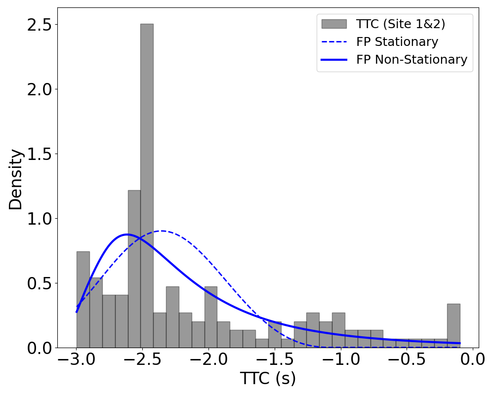
(a) FP with stationary and non-stationary

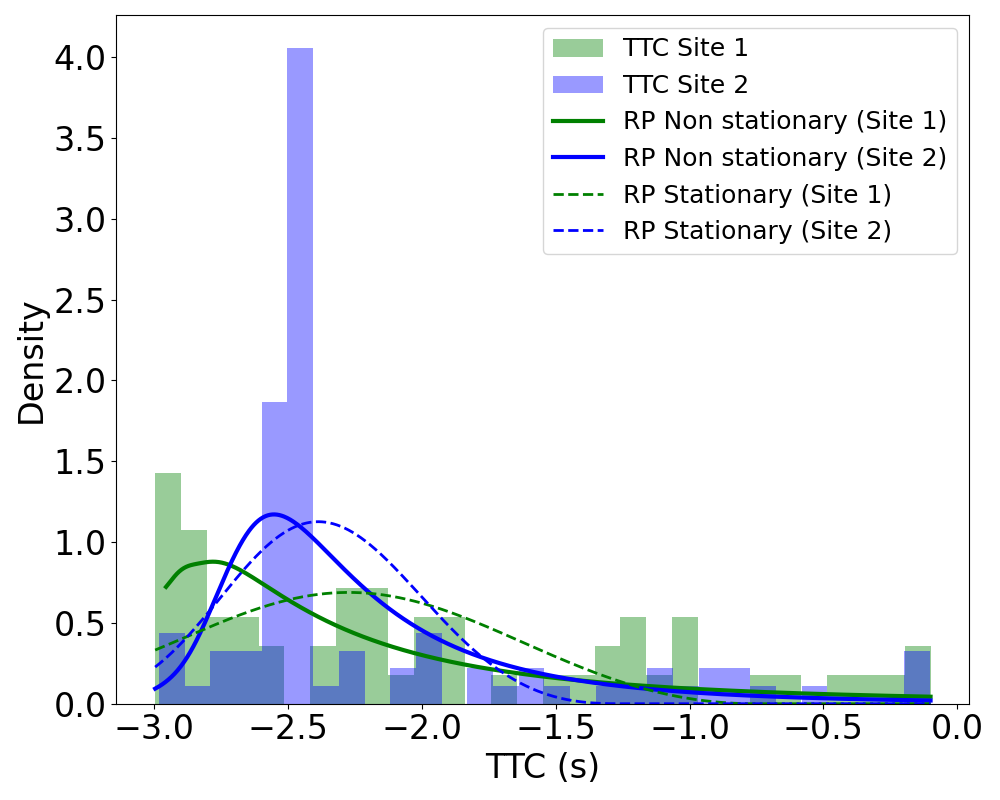
(b) RP with stationary and non-stationary

Fig. 10.: Posterior predictive model check for San Francisco sites

After ensuring proper sampling with minimal autocorrelation, model fit was checked using posterior predictive checks by comparing model data with observations (Gelman et al., 1996). Samples drawn from the posterior distribution generated data using the likelihood function. The posterior predictive model checks, illustrated in Figures: 4.2, 4.2, and 4.2, visualize that non-stationary models consistently outperform stationary models, highlighting the importance of accounting for random effects and temporal variations. These figures show that non-stationary models provide better predictions of extreme values than stationary models, especially the HBSRP model, closely matching observed data, indicating a better fit. The sign and magnitude of the mean estimates of covariates in (Table: 3, 4, and 5) can be used to interpret their impact on overall crash risk.

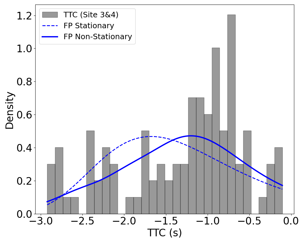
(a) FP with stationary and non-stationary

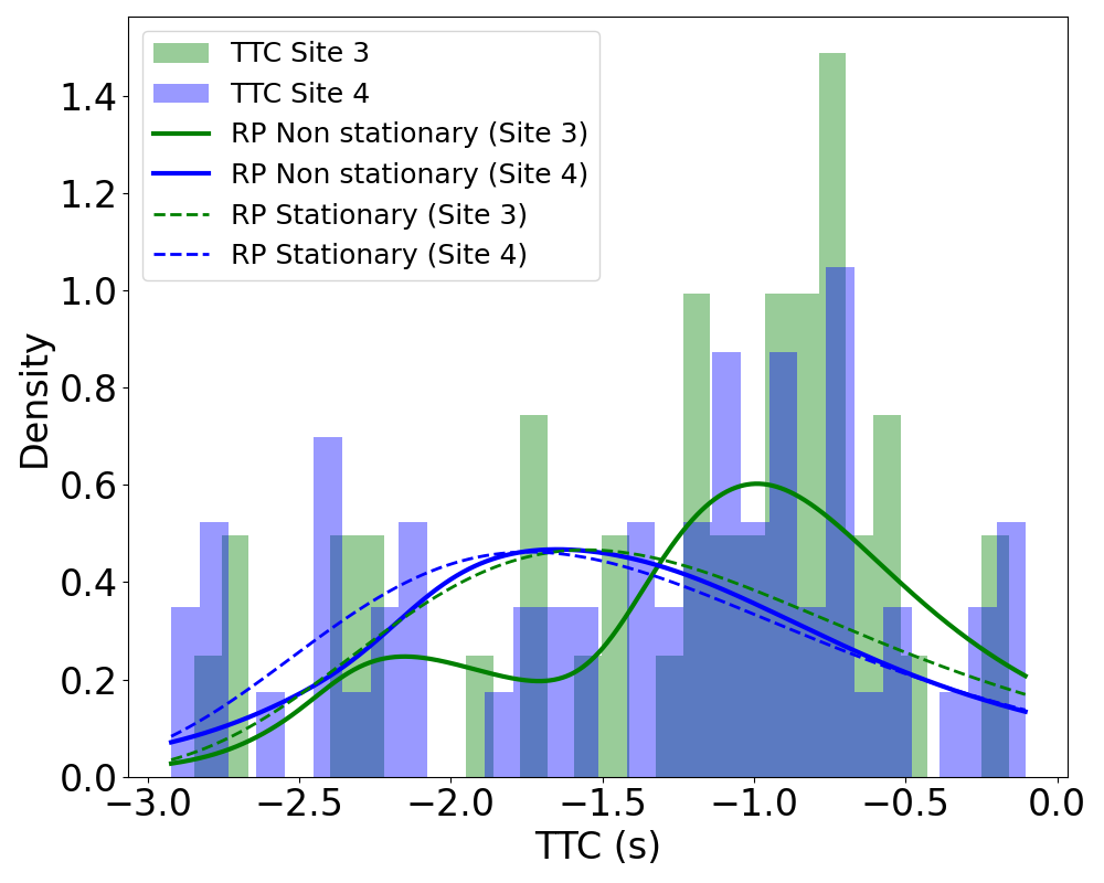
(b) RP with stationary and non-stationary

Fig. 11.: Posterior predictive model check for Phoenix sites

In San Francisco, the HBSRP model significantly outperformed others, with a DIC difference greater than ten compared to other models. For Phoenix and Los Angeles, the differences in DIC values between fixed parameter (FP) and RP non-stationary models were greater than five. Despite these variations, the RP non-stationary model (HBSRP) consistently reported the lowest DIC values for all city datasets, indicating a superior fit across cities. These models effectively capture the unobserved heterogeneity in traffic conflict sites by allowing parameters to vary across observations, accommodating the inherent variability in traffic dynamics. The non-stationary nature of these models will enable them to adapt to temporal and spatial changes, reflecting real-world conditions more accurately. Using MCMC algorithms, the models achieve improved parameter estimation, especially when individual vehicle dynamics are included as covariates, resulting in more precise and reliable crash risk predictions. The hierarchical Bayesian structure further enhances the model fit by distinguishing between within-site and between-site variability. At the same time, the extreme value distribution focuses on rare but significant events, crucial for assessing high-risk scenarios.

The analysis of model estimation results reveals significant associations between vehicle dynamics and the GEV distribution parameters for TTC across different cities. In San Francisco (Table:3), the speed of vehicle-2 and the acceleration of vehicle-1 are significantly linked to the location parameter, while the speed and acceleration of vehicle-2 are significantly related to the scale parameter. Here, vehicle-1 and vehicle-2 are represented in Fig. 3.2. In Phoenix (Table: 4), the speeds of both vehicle-1 and 2 significantly affect the location parameter, and the speed and acceleration of vehicle-1, along with the speed of vehicle-2, influence the scale parameter. For the Los Angeles sites (Table: 5), the speed of vehicle-1 and the acceleration of vehicle-2 are significantly associated with the location parameter, but no covariates significantly impact the scale parameter. The HBSRP model results confirm that the variances of the parameter distributions for the intercept random coefficient of the GEV distribution for TTC are statistically appropriate for the location, shape, and scale parameters.

Our comprehensive analysis provides both theoretical insights and practical implications. Non-stationary models with random parameters consistently outperform stationary models, highlighting the importance of considering temporal variations and random effects in predicting traffic conflicts and crash risks. The unique traffic conflict patterns observed in different locations necessitate tailored safety interventions. The EVT models with a hierarchical Bayesian structure effectively capture the extreme values and tail behavior of conflict distributions, which is crucial for assessing high-risk scenarios. The significant differences between stationary and non-stationary models underscore the need to account for time-varying factors in traffic safety analysis. Random parameters enhance model flexibility and performance, capturing unobserved heterogeneity among different locations. These insights provide a robust framework for understanding traffic conflict dynamics and implementing proactive safety measures.

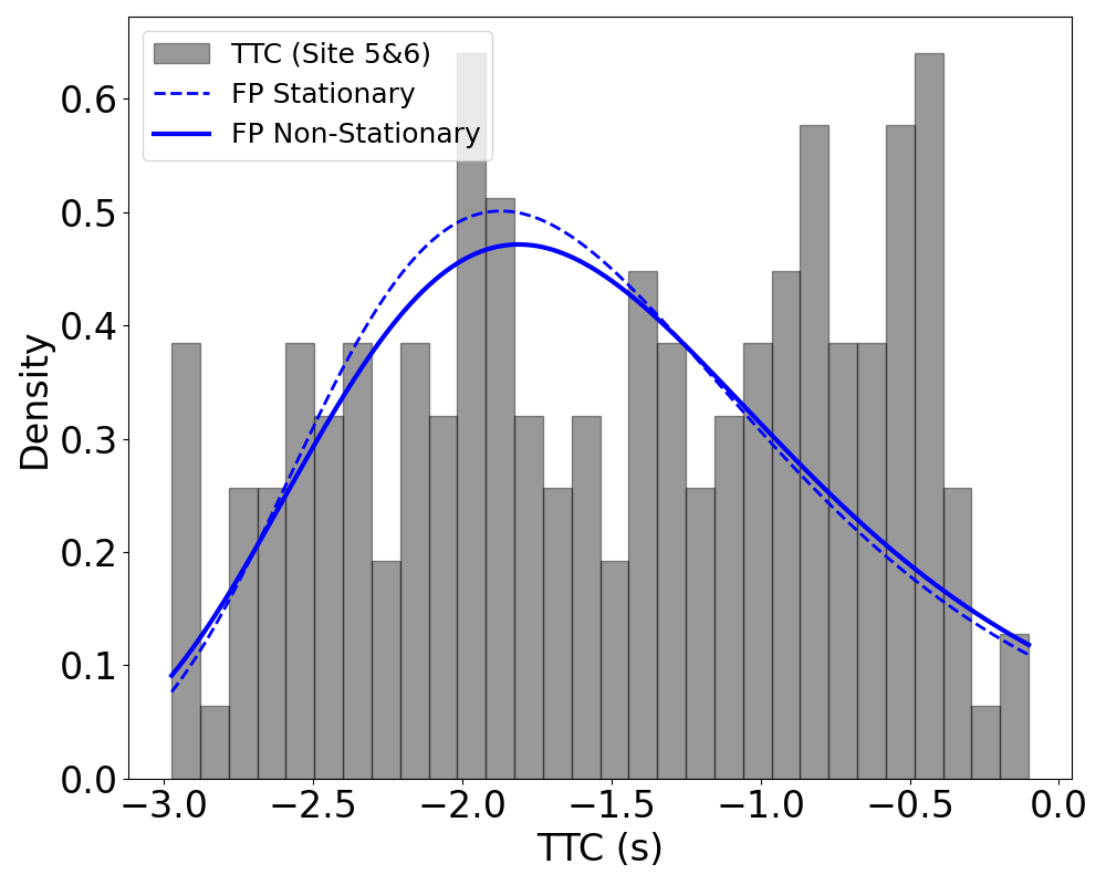
(a) FP with stationary and non-stationary

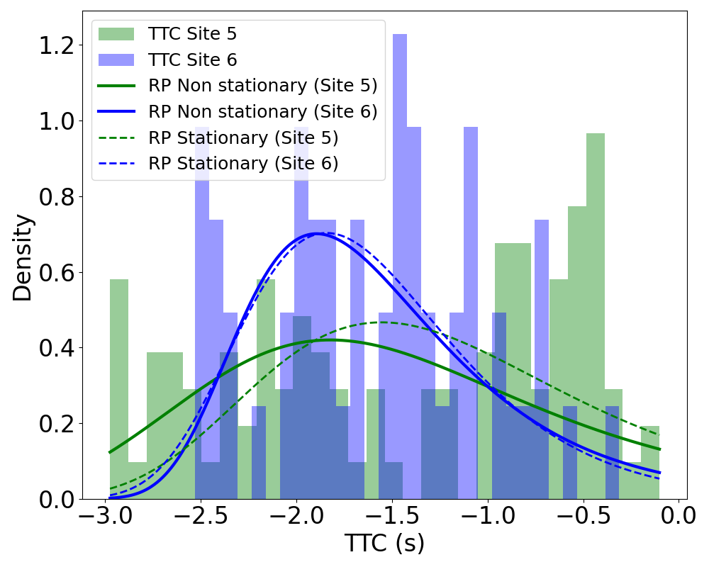
(b) RP with stationary and non-stationary

Fig. 12.: Posterior predictive model check for Los Angeles sites

4.3 Model validation

To validate the performance of the HBSRP model, this study estimates near misses frequency (C) at different thresholds ($\lambda$) using Eqn. 23, which is derived from Eqn. 16 . The estimation is performed by summing the probabilities that the maximum conflict value ($X_{n}$) in each time block exceeds the threshold ($\lambda$). The formula for the estimated frequencies of extreme conflicts is given by:

$$C_{m\lambda}=\begin{cases}\sum_{n=1}^{k}\left(1-\exp\left[-\left(1-\xi_{n}\frac{\lambda-\mu_{n}}{\exp(\vartheta_{n})}\right)^{-1/\xi_{n}}\right]\right),&\text{for }\xi_{n}\neq 0\\ \sum_{n=1}^{k}\left(1-\exp\left[-\exp\left(\frac{\lambda-\mu_{n}}{\exp(\vartheta_{n})}\right)\right]\right),&\text{for }\xi_{n}=0\end{cases}$$ (23)

In this formula, $m$ denotes the site type, $\lambda$ represents the threshold values (-0.2, to -0.9), and $k$ is the number of blocks for each site. The parameters $\mu_{n}$, $\vartheta_{n}$, and $\xi_{n}$ are the location, scale, and shape parameters of the GEV distribution, respectively. To calibrate the model’s parameters, we split the dataset into training and test datasets for model validation. The training dataset is used to calibrate the parameters, while the test dataset is used to assess the model’s performance. This estimation allows us to compute the expected number of extreme near misses for different severity levels and compare these estimates with the observed near miss frequencies to assess the model’s predictive accuracy. Table 6 comprehensively compares observed and estimated near-miss incidents across six different sites and thresholds ranging from -0.2 to -0.9, highlighting key insights into the model’s predictive performance. Each cell in the table displays the estimated near misses, followed by the observed near misses in parentheses. The model overestimates near misses at severe thresholds, suggesting that the model may be overly sensitive at these severe thresholds, leading to higher predicted values than found near misses using Eqn. 5 and 6. Conversely, the model underestimates the near misses at less severe thresholds, which indicates that the model is restricted to accurately predicting the number of near misses under less severe conditions. Figure 4.3 shows that the estimated mean values for most sites are generally higher than the observed value. The confidence intervals indicate the range within which the true number of near misses is expected to lie in 95% confidence. The model seems to provide reasonable estimates, although there are instances where the observed near-misses fall outside the estimated confidence intervals.

Table 6: Estimated and observed near misses at different sites and thresholds

${\lambda}$ (sec)	Site 1	Site 2	Site 3	Site4	Site 5	Site 6
-0.2	0.67 (0)	0.43 (1)	0.6 (0)	2.0 (1)	0.9 (0)	0.2 (0)
-0.3	1.3 (1)	0.98 (1)	1.8 (1)	2.4 (1)	1.9 (2)	0.4 (0)
-0.4	2.5 (2)	1.9 (1)	3.2 (1)	2.5 (3)	3.5 (3)	0.9 (0)
-0.5	3.9 (3)	2.9 (1)	4.7 (1)	3.9 (3)	5.6 (6)	1.4 (1)
-0.6	4.7 (3)	4.1 (1)	6.9 (2)	5.7 (4)	9.8 (11)	1.9 (1)
-0.7	5.7 (3)	6.2 (2)	9.7 (3)	7.9 (5)	16.7 (23)	2.8 (2)
-0.8	6.6 (4)	7.8 (4)	11.8 (8)	12.3 (9)	24.5 (28)	3.2 (2)
-0.9	8.2 (5)	9.2 (5)	13.7 (14)	17.6 (15)	29.8 (34)	4.8 (3)

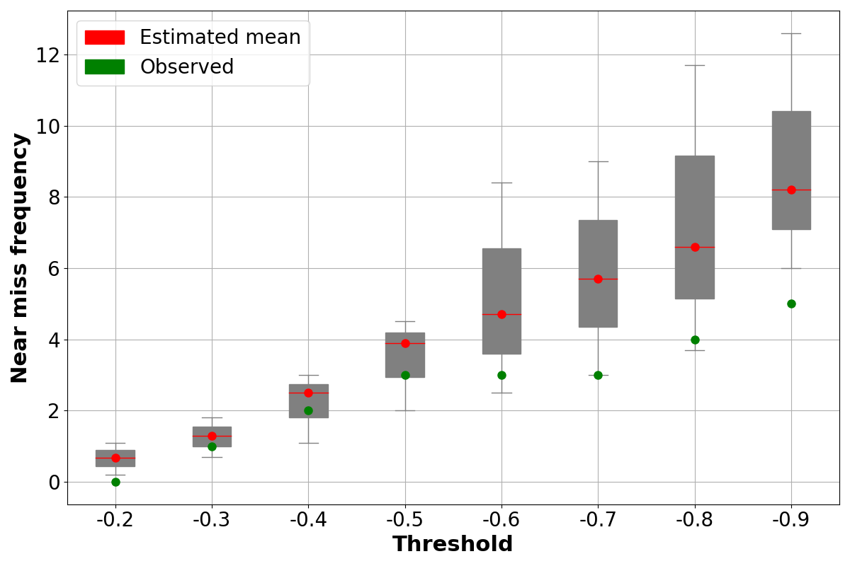
(a) Site-1

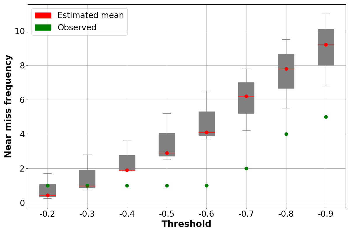
(b) Site-2

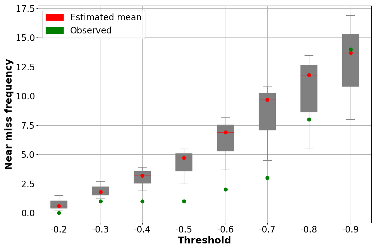
(c) Site-3

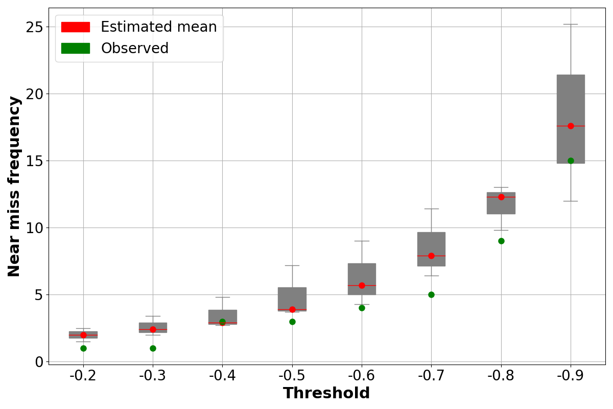
(d) Site-4

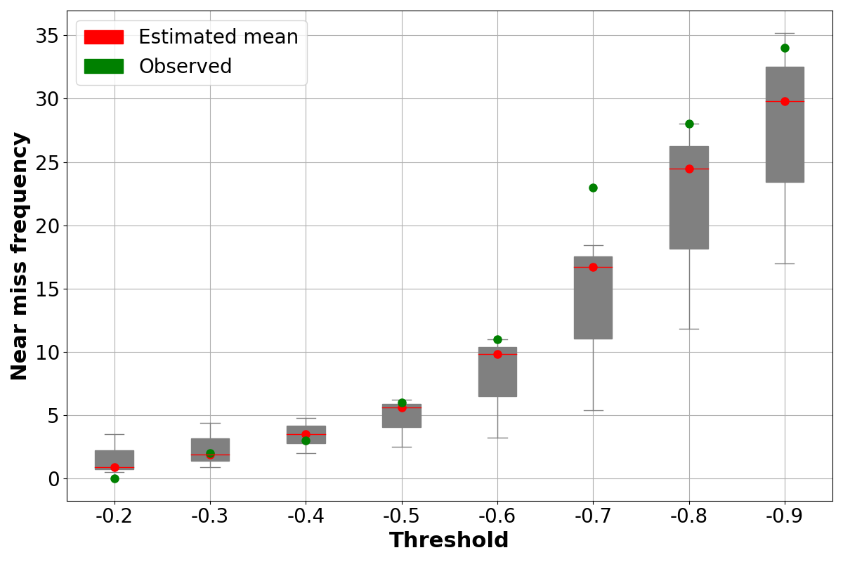
(e) Site-5

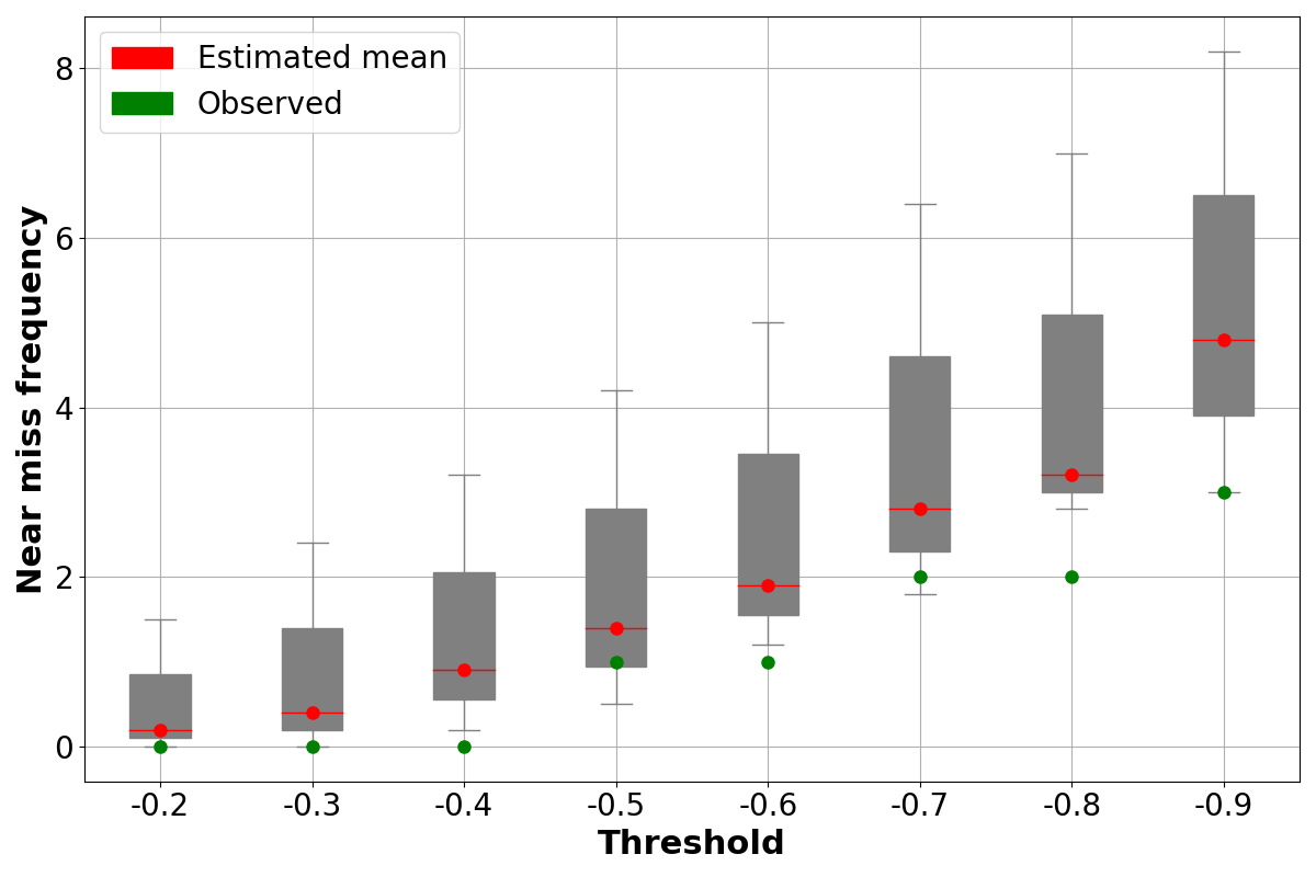
(f) Site-6

Fig. 13.: Result comparison of observed and estimated near miss using HBSRP model

5 Discussion

This study developed a real-time framework for estimating HDV near-miss risks using Waymo AV sensor data, including high-resolution HDV vehicle trajectories. The framework employs hierarchical Bayesian EVT models with block minima sampling approaches. A suitable risk indicator is crucial for effective near-miss-based traffic safety assessments, ensuring alignment with the study’s specific objectives and purposes. This study chose a 2D-based TTC risk indicator to estimate near misses from HDV-HDV interactions, as HDVs often follow 2D paths during maneuvers such as merging, lane changes, passing, etc. While this study focuses on TTC as the single risk indicator, future research can explore other 2D risk indicators such as PET, DRAC, MTTC, etc.

This risk indicator TTC, developed by Li et al.(2024), is derived from SSM and is integrated into the GEV framework. This allows for estimating the risk associated with HDV interactions across various highway geometries while accounting for vehicle dynamics and fidelity. Unlike most existing literature, this study calculated TTC based on vehicle longitudinal and steering movements to identify vehicle near-miss extreme events. These extremes were then fitted using GEV distributions to estimate near-miss frequency. The study also explored whether the identified extremes fit better with stationary or non-stationary GEV distributions. Among the four GEV models estimated, the non-stationary model for both location and scale with random parameters (HBSRP) performed best using the block minima approach. The developed model was validated through training and test datasets, which produced mean predicted near misses that closely matched observed near misses and demonstrated narrower confidence intervals, indicating higher precision and reliability in risk estimation.

While Waymo AV traverses roadways, their LiDAR sensors collect trajectories on nearby road users, including HDVs. Despite the limited sample size due to the low penetration rate and short duration of each segment, the high-resolution data is valuable for capturing the dynamic nature of HDVs. Consequently, the number of HDV-HDV conflict pairs was relatively limited during the observation period. This limited sample size may have resulted in wide confidence intervals in the HBSRP model. Fu and Sayed (2023) found that larger observation sample sizes in the hierarchical Bayesian GEV model led to lower model uncertainty. They proposed a method for identifying an adequate sample size for conflict-based crash risk estimation models, which was applied to the hierarchical Bayesian GEV model. The framework developed in this study generated the nearest accurate near-miss estimates and their confidence intervals, even with a relatively short observation period. However, the confidence intervals remained notably wide, likely due to the small sample size resulting from the brief observation period. To address this, future studies could extend the observation periods for specific conflict types and enhance the precision of risk estimates. Therefore, a comprehensive investigation into how varying observation periods affect the accuracy and confidence intervals of risk estimates for HDV is warranted. However, using a large block size often results in a high variance in model parameters (Ali et al., 2022).

The non-stationarity in the extreme value models was addressed by parameterizing the location and scale parameters using relevant covariates and incorporating random intercepts. Specifically, the block minima approach utilized covariates such as conflicting vehicle speed and acceleration to capture the dynamic nature of the data. Studies have highlighted the importance of incorporating vehicular heterogeneity in crash risk assessment (Kumar and Mudgal, 2024). This is particularly relevant in HDV crashes, where vehicle speeds and accelerations are key indicators of surrounding road traffic situations (Fu and Sayed, 2021). The model with these covariates outperformed competing models, as demonstrated by local and global goodness-of-fit measures. This superior performance indicates that including these specific covariates significantly enhanced the model’s ability to predict crash risks accurately, providing a more precise and reliable assessment of vehicle dynamics and near-miss events. First, a local goodness-of-fit measure was performed by comparing probability density plots (empirical versus modeled). The results showed that the conflict extremes identified by HBSRP follow extreme value distributions, indicating their suitability as an alternative to other modeling approaches.

Given the lack of a definitive ground truth for identifying real extremes in the Waymo dataset, a cross-fold approach was adopted. The dataset was divided into training and test datasets to evaluate the performance of the HBSRP modeling approach. Global GOF measures, such as mean near-miss, which may be overly sensitive estimates and confidence intervals, were used to assess the model’s performance. The model overestimates near misses at severe thresholds, suggesting it may be overly sensitive. Conversely, the model underestimates near misses at less severe thresholds, indicating a limitation in predicting the number of near misses under these conditions. It was also found that the mean near-miss estimates for block minima, fitted to GEV distributions, fell outside the confidence intervals of the observed near misses at some sites, indicating a potential limitation in the model’s accuracy.

6 Summary and Conclusions

This study introduced a pioneering framework for real-time near-miss risk estimation using sensor data from AVs and EVT within a hierarchical Bayesian structure. It focused on near-miss events and provided a more dynamic and proactive approach to traffic safety analysis. The methodology incorporated SSM-based 2D risk indicator TTC and highlighted the significance of considering vehicle dynamics heterogeneity, specifically the interactions between HDV-HDV. The study acknowledged the heterogeneous nature of traffic, considering the distinct states of interacting vehicles and their impact on near-miss risk. By evaluating exogenous variables such as vehicle speed and acceleration, it identified key factors contributing to higher near-miss risk probabilities. The hierarchical Bayesian structure enhanced the precision of risk estimation by capturing unobserved heterogeneity and temporal variations across different sites. GEV models effectively represented extreme values and tail behavior of extreme event distributions, which was crucial for assessing high-risk scenarios. This approach provides a nuanced understanding of the dynamic interplay between potentially conflicting vehicles, contributing to more accurate risk predictions. By leveraging high-resolution Waymo sensor data, the study offered detailed insights into vehicle interactions and traffic near-miss risk dynamics, paving the way for proactive traffic management and safety measures. The study successfully demonstrated the suitability of the proposed framework for estimating HDV-HDV intersection risk using high-fidelity vehicle movement models. This study was among the first to apply open-source, high-resolution AV sensor data to conduct real-time vehicle safety analysis with a high-fidelity 2D analytical framework considering individual vehicle dynamics. As shown by Li et al. (2024), transitioning from conventional 1D crash risk models to more complex 2D models improved the accuracy of real-time safety analyses. The framework’s modular and scalable nature allowed for its application to larger problem sets such as digital twins, demonstrating its potential for extensive active safety research. Future research can explore multivariate EVT models to predict HDV-HDV near-miss risk with severity and consider various conflict measures to characterize vehicle interactions comprehensively. Without delving into individual collision types, the study’s focus on generalized sites and conflict types suggested an avenue for future work to investigate different collision types and road-user interactions. As AV penetration increases, the data collection will enable more in-depth safety research, addressing macroscopic phenomena and variations in road geometry characteristics. This study laid the foundation for enhancing road safety and reducing crash occurrences through informed, data-driven interventions.

Acknowledgement:

This research is funded by Federal Highway Administration (FHWA) Exploratory Advanced Research 693JJ323C000010. The results do not reflect FHWA’s opinions.

Disclaimer:

The results presented in this document do not necessarily reflect those from the Federal Highway Administration.

Data availability:

Data and code will be made available on reasonable request.

References

- Abdel-Aty et al. 2010 Abdel-Aty, M., Pande, A., Hsia, L., 2010. The concept of proactive traffic management for enhancing freeway safety and operation. ITE journal 80, 34.
- Abdel-Aty et al. 2023a Abdel-Aty, M., Wang, Z., Zheng, O., Abdelraouf, A., 2023a. Advances and applications of computer vision techniques in vehicle trajectory generation and surrogate traffic safety indicators. arXiv preprint arXiv:2303.15231 .
- Abdel-Aty et al. 2023b Abdel-Aty, M., Zheng, O., Wu, Y., Abdelraouf, A., Rim, H., Li, P., 2023b. Real-time big data analytics and proactive traffic safety management visualization system. Journal of transportation engineering, Part A: Systems 149, 04023064.
- Ali et al. 2023 Ali, Y., Haque, M.M., Mannering, F., 2023. Assessing traffic conflict/crash relationships with extreme value theory: Recent developments and future directions for connected and autonomous vehicle and highway safety research. Analytic methods in accident research , 100276.
- Ali et al. 2022 Ali, Y., Haque, M.M., Zheng, Z., 2022. Assessing a connected environment’s safety impact during mandatory lane-changing: A block maxima approach. IEEE Transactions on Intelligent Transportation Systems .
- Allen et al. 1978 Allen, B.L., Shin, B.T., Cooper, P.J., 1978. Analysis of traffic conflicts and collisions. Technical Report.
- Arun et al. 2021 Arun, A., Haque, M.M., Bhaskar, A., Washington, S., Sayed, T., 2021. A systematic mapping review of surrogate safety assessment using traffic conflict techniques. Accident Analysis & Prevention 153, 106016.
- Bücher and Zhou 2021 Bücher, A., Zhou, C., 2021. A horse race between the block maxima method and the peak–over–threshold approach. Statistical Science 36, 360–378.
- Coles et al. 2001 Coles, S., Bawa, J., Trenner, L., Dorazio, P., 2001. An introduction to statistical modeling of extreme values. volume 208. Springer.
- Cooley et al. 2006 Cooley, D., Naveau, P., Jomelli, V., Rabatel, A., Grancher, D., 2006. A bayesian hierarchical extreme value model for lichenometry. Environmetrics: The official journal of the International Environmetrics Society 17, 555–574.
- Dai et al. 2023 Dai, Y., Wang, C., Xie, Y., 2023. Explicitly incorporating surrogate safety measures into connected and automated vehicle longitudinal control objectives for enhancing platoon safety. Accident Analysis & Prevention 183, 106975.
- Das et al. 2022 Das, T., Samandar, M.S., Rouphail, N., 2022. Longitudinal traffic conflict analysis of autonomous and traditional vehicle platoons in field tests via surrogate safety measures. Accident Analysis & Prevention 177, 106822.
- Davis et al. 2011 Davis, G.A., Hourdos, J., Xiong, H., Chatterjee, I., 2011. Outline for a causal model of traffic conflicts and crashes. Accident Analysis & Prevention 43, 1907–1919.
- El-Basyouny and Sayed 2009 El-Basyouny, K., Sayed, T., 2009. Urban arterial accident prediction models with spatial effects. Transportation research record 2102, 27–33.
- Essa and Sayed 2020 Essa, M., Sayed, T., 2020. Comparison between surrogate safety assessment model and real-time safety models in predicting field-measured conflicts at signalized intersections. Transportation research record 2674, 100–112.
- Ettinger et al. 2021 Ettinger, S., Cheng, S., Caine, B., Liu, C., Zhao, H., Pradhan, S., Chai, Y., Sapp, B., Qi, C.R., Zhou, Y., et al., 2021. Large scale interactive motion forecasting for autonomous driving: The waymo open motion dataset, in: Proceedings of the IEEE/CVF International Conference on Computer Vision, pp. 9710–9719.
- Ferreira and De Haan 2015 Ferreira, A., De Haan, L., 2015. On the block maxima method in extreme value theory: Pwm estimators. The Annals of statistics , 276–298.
- Fu and Sayed 2021 Fu, C., Sayed, T., 2021. Random parameters bayesian hierarchical modeling of traffic conflict extremes for crash estimation. Accident Analysis & Prevention 157, 106159.
- Fu and Sayed 2022a Fu, C., Sayed, T., 2022a. Bayesian dynamic extreme value modeling for conflict-based real-time safety analysis. Analytic methods in accident research 34, 100204.
- Fu and Sayed 2022b Fu, C., Sayed, T., 2022b. Random-parameter bayesian hierarchical extreme value modeling approach with heterogeneity in means and variances for traffic conflict–based crash estimation. Journal of transportation engineering, Part A: Systems 148, 04022056.
- Fu and Sayed 2023 Fu, C., Sayed, T., 2023. Identification of adequate sample size for conflict-based crash risk evaluation: an investigation using bayesian hierarchical extreme value theory models. Analytic methods in accident research 39, 100281.
- Fu et al. 2020 Fu, C., Sayed, T., Zheng, L., 2020. Multivariate bayesian hierarchical modeling of the non-stationary traffic conflict extremes for crash estimation. Analytic methods in accident research 28, 100135.
- Gelman et al. 1996 Gelman, A., Meng, X.L., Stern, H., 1996. Posterior predictive assessment of model fitness via realized discrepancies. Statistica sinica , 733–760.
- Gelman and Rubin 1992 Gelman, A., Rubin, D.B., 1992. Inference from iterative simulation using multiple sequences. Statistical science 7, 457–472.
- Ghoul et al. 2023 Ghoul, T., Sayed, T., Fu, C., 2023. Dynamic identification of short-term and longer-term hazardous locations using a conflict-based real-time extreme value safety model. Analytic methods in accident research 37, 100262.
- Hayward 1971 Hayward, J., 1971. Near misses as a measure of safety at urban intersections. Pennsylvania Transportation and Traffic Safety Center.
- Hu et al. 2023 Hu, X., Zheng, Z., Zhang, X., Chen, D., Sun, J., 2023. Vehicle trajectory data processed from the Waymo Open Dataset. Technical Report. Mendeley Data. doi:10.17632/wfn2c3437n.3.
- Kamel et al. 2023 Kamel, A., Sayed, T., Fu, C., 2023. Real-time safety analysis using autonomous vehicle data: a bayesian hierarchical extreme value model. Transportmetrica B: Transport Dynamics 11, 826–846.
- Kamel et al. 2024 Kamel, A., Sayed, T., Kamel, M., 2024. Real-time combined safety-mobility assessment using self-driving vehicles collected data. Accident Analysis & Prevention 199, 107513.
- Kim et al. 2024 Kim, Y., Kang, K., Park, J., Oh, C., 2024. A methodology for prioritizing safety indicators using individual vehicle trajectory data. Journal of Transportation Safety & Security 16, 18–42.
- Kumar and Mudgal 2024 Kumar, A., Mudgal, A., 2024. Risk assessment of rear-end crashes by incorporating vehicular heterogeneity into bayesian hierarchical extreme value models. Transportmetrica B: Transport Dynamics 12, 2323058.
- Lee et al. 2017 Lee, J., Abdel-Aty, M., Cai, Q., 2017. Intersection crash prediction modeling with macro-level data from various geographic units. Accident Analysis & Prevention 102, 213–226.
- Li et al. 2024 Li, S., Anis, M., Lord, D., Zhang, H., Zhou, Y., Ye, X., 2024. Beyond 1d and oversimplified kinematics: A generic analytical framework for surrogate safety measures. Accident Analysis & Prevention 204, 107649.
- Lord et al. 2021 Lord, D., Qin, X., Geedipally, S.R., 2021. Highway safety analytics and modeling. Elsevier.
- Lu et al. 2022 Lu, J., Grembek, O., Hansen, M., 2022. Learning the representation of surrogate safety measures to identify traffic conflict. Accident Analysis & Prevention 174, 106755.
- Mannering 2018 Mannering, F., 2018. Temporal instability and the analysis of highway accident data. Analytic methods in accident research 17, 1–13.
- Mannering et al. 2020 Mannering, F., Bhat, C.R., Shankar, V., Abdel-Aty, M., 2020. Big data, traditional data and the tradeoffs between prediction and causality in highway-safety analysis. Analytic methods in accident research 25, 100113.
- Mannering et al. 2016 Mannering, F.L., Shankar, V., Bhat, C.R., 2016. Unobserved heterogeneity and the statistical analysis of highway accident data. Analytic methods in accident research 11, 1–16.
- Minderhoud and Bovy 2001 Minderhoud, M.M., Bovy, P.H., 2001. Extended time-to-collision measures for road traffic safety assessment. Accident Analysis & Prevention 33, 89–97.
- National Safety Council 2021 National Safety Council, 2021. 2021 motor-vehicle crash highlights. https://injuryfacts.nsc.org/motor-vehicle/overview/introduction. Accessed on: 2023-11-29.
- NHTSA 2021 NHTSA, 2021. Nhtsa estimates for 2022 show roadway fatalities remain flat after two years of dramatic increases. URL: https://www.nhtsa.gov/press-releases/traffic-crash-death-estimates-2022.
- Oikonomou et al. 2023 Oikonomou, M.G., Ziakopoulos, A., Chaudhry, A., Thomas, P., Yannis, G., 2023. From conflicts to crashes: Simulating macroscopic connected and automated driving vehicle safety. Accident Analysis & Prevention 187, 107087.
- Orsini et al. 2019 Orsini, F., Gecchele, G., Gastaldi, M., Rossi, R., 2019. Collision prediction in roundabouts: a comparative study of extreme value theory approaches. Transportmetrica A: transport science 15, 556–572.
- Orsini et al. 2020 Orsini, F., Gecchele, G., Gastaldi, M., Rossi, R., 2020. Large-scale road safety evaluation using extreme value theory. IET Intelligent Transport Systems 14, 1004–1012.
- Ozbay et al. 2008 Ozbay, K., Yang, H., Bartin, B., Mudigonda, S., 2008. Derivation and validation of new simulation-based surrogate safety measure. Transportation research record 2083, 105–113.
- Pei et al. 2011 Pei, X., Wong, S., Sze, N.N., 2011. A joint-probability approach to crash prediction models. Accident Analysis & Prevention 43, 1160–1166.
- Perkins and Harris (1967 Perkins, S.R., Harris, J.I., (1967). Traffic conflict characteristics: Freeway curve and exit area f1, december, 1966. .
- Rahman and Abdel-Aty 2018 Rahman, M.S., Abdel-Aty, M., 2018. Longitudinal safety evaluation of connected vehicles’ platooning on expressways. Accident Analysis & Prevention 117, 381–391.
- Sayed et al. 2010 Sayed, T., Saunier, N., Lovegrove, G., de Leur, P., 2010. Advances in proactive road safety planning, in: Proceedings of the 20th Canadian Multidisciplinary Road Safety Conference (Niagara Falls, Ontario).
- Singh 2018 Singh, S., 2018. Critical Reasons for Crashes Investigated in the National Motor Vehicle Crash Causation Survey. Technical Report.
- Songchitruksa and Tarko 2006 Songchitruksa, P., Tarko, A.P., 2006. The extreme value theory approach to safety estimation. Accident Analysis & Prevention 38, 811–822.
- St-Aubin et al. 2013 St-Aubin, P., Miranda-Moreno, L., Saunier, N., 2013. An automated surrogate safety analysis at protected highway ramps using cross-sectional and before–after video data. Transportation Research Part C: Emerging Technologies 36, 284–295.
- Tarko 2018a Tarko, A.P., 2018a. Estimating the expected number of crashes with traffic conflicts and the lomax distribution–a theoretical and numerical exploration. Accident Analysis & Prevention 113, 63–73.
- Tarko 2018b Tarko, A.P., 2018b. Surrogate measures of safety, in: Safe mobility: challenges, methodology and solutions. Emerald Publishing Limited. volume 11, pp. 383–405.
- Varhelyi 1998 Varhelyi, A., 1998. Drivers’ speed behaviour at a zebra crossing: a case study. Accident Analysis & Prevention 30, 731–743.
- Venthuruthiyil and Chunchu 2022 Venthuruthiyil, S.P., Chunchu, M., 2022. Anticipated collision time (act): A two-dimensional surrogate safety indicator for trajectory-based proactive safety assessment. Transportation research part C: emerging technologies 139, 103655.
- Vogel 2003 Vogel, K., 2003. A comparison of headway and time to collision as safety indicators. Accident analysis & prevention 35, 427–433.
- Wang and Stamatiadis 2014 Wang, C., Stamatiadis, N., 2014. Evaluation of a simulation-based surrogate safety metric. Accident Analysis & Prevention 71, 82–92.
- Wang et al. 2021 Wang, C., Xie, Y., Huang, H., Liu, P., 2021. A review of surrogate safety measures and their applications in connected and automated vehicles safety modeling. Accident Analysis & Prevention 157, 106157.
- Wang et al. 2019 Wang, C., Xu, C., Dai, Y., 2019. A crash prediction method based on bivariate extreme value theory and video-based vehicle trajectory data. Accident Analysis & Prevention 123, 365–373.
- Yang et al. 2022 Yang, D., Ozbay, K., Gao, J., Zuo, F., 2022. A functional approach for analyzing time-dependent driver response behavior to real-world connected vehicle warnings. IEEE Transactions on Intelligent Transportation Systems 24, 3438–3447.
- Yang et al. 2021 Yang, D., Ozbay, K., Xie, K., Yang, H., Zuo, F., Sha, D., 2021. Proactive safety monitoring: A functional approach to detect safety-related anomalies using unmanned aerial vehicle video data. Transportation research part C: emerging technologies 127, 103130.
- Yuan et al. 2018a Yuan, J., Abdel-Aty, M., Wang, L., Lee, J., Wang, X., Yu, R., 2018a. Real-time crash risk analysis of urban arterials incorporating bluetooth, weather, and adaptive signal control data. arXiv preprint arXiv:1805.07826 .
- Yuan et al. 2018b Yuan, J., Abdel-Aty, M., Wang, L., Lee, J., Yu, R., Wang, X., 2018b. Utilizing bluetooth and adaptive signal control data for real-time safety analysis on urban arterials. Transportation research part C: emerging technologies 97, 114–127.
- Yue et al. 2018 Yue, L., Abdel-Aty, M., Wu, Y., Wang, L., 2018. Assessment of the safety benefits of vehicles’ advanced driver assistance, connectivity and low level automation systems. Accident Analysis & Prevention 117, 55–64.
- Zhang et al. 2019 Zhang, H., Liptrott, M., Bessis, N., Cheng, J., 2019. Real-time traffic analysis using deep learning techniques and uav based video, in: 2019 16th IEEE International Conference on Advanced Video and Signal Based Surveillance (AVSS), IEEE. pp. 1–5.
- Zhang et al. 2020 Zhang, J., Wu, K., Cheng, M., Yang, M., Cheng, Y., Li, S., 2020. Safety evaluation for connected and autonomous vehicles’ exclusive lanes considering penetrate ratios and impact of trucks using surrogate safety measures. Journal of advanced transportation 2020, 1–16.
- Zheng et al. 2014 Zheng, L., Ismail, K., Meng, X., 2014. Freeway safety estimation using extreme value theory approaches: A comparative study. Accident Analysis & Prevention 62, 32–41.
- Zheng and Sayed 2019 Zheng, L., Sayed, T., 2019. Application of extreme value theory for before-after road safety analysis. Transportation research record 2673, 1001–1010.
- Zhu et al. 2023 Zhu, C., Brown, C.T., Dadashova, B., Ye, X., Sohrabi, S., Potts, I., 2023. Investigation on the driver-victim pairs in pedestrian and bicyclist crashes by latent class clustering and random forest algorithm. Accident Analysis & Prevention 182, 106964.