AI-Enhanced 7-Point Checklist for Melanoma Detection Using Clinical Knowledge Graphs and Data-Driven Quantification

Abstract

The 7-point checklist (7PCL) is widely used in dermoscopy to identify malignant melanoma lesions needing urgent medical attention. It assigns point values to seven attributes: major attributes are worth two points each, and minor ones are worth one point each. A total score of three or higher prompts further evaluation, often including a biopsy. However, a significant limitation of current methods is the uniform weighting of attributes, which leads to imprecision and neglects their interconnections. Previous deep learning studies have treated the prediction of each attribute with the same importance as predicting melanoma, which fails to recognize the clinical significance of the attributes for melanoma. To address these limitations, we introduce a novel diagnostic method that integrates two innovative elements: a Clinical Knowledge-Based Topological Graph (CKTG) and a Gradient Diagnostic Strategy with Data-Driven Weighting Standards (GD-DDW). The CKTG integrates 7PCL attributes with diagnostic information, revealing both internal and external associations. By employing adaptive receptive domains and weighted edges, we establish connections among melanoma’s relevant features. Concurrently, GD-DDW emulates dermatologists’ diagnostic processes, who first observe the visual characteristics associated with melanoma and then make predictions. Our model uses two imaging modalities for the same lesion, ensuring comprehensive feature acquisition. Our method shows outstanding performance in predicting malignant melanoma and its features, achieving an average AUC value of 85%. This was validated on the EDRA dataset, the largest publicly available dataset for the 7-point checklist algorithm. Specifically, the integrated weighting system can provide clinicians with valuable data-driven benchmarks for their evaluations.

Melanoma, 7-point checklist, data-driven, classification, multi-modal

1 Introduction

Skin cancer is a widespread malignancy worldwide, with melanoma being the most dangerous type. Although the incidence of skin cancer varies by region and individual risk factors, timely diagnosis and prompt intervention can significantly improve the prognosis of the disease [1].

In the medical field, healthcare professionals utilize diverse imaging modalities to expedite the diagnosis and treatment of skin lesions [2]. Two notable techniques are dermoscopic imaging and clinical photography. Dermoscopy, which is an optical magnification technique assisted by liquid immersion and cross-polarized illumination, produces intricate images revealing subepidermal structures and lesions to support the diagnosis [3]. On the other hand, clinical images efficiently capture essential morphological features including color, texture, shape, and borders, despite their inability to explore intricate subcutaneous lesion details. The convenience and accessibility of clinical images, especially through widely available mobile electronic devices like smartphones, are indisputable benefits [4]. The fusion of these two imaging techniques provides a comprehensive information essential in practical medical scenarios, specifically for melanoma diagnosis.

Figure 1: Example of biopsy-confirmed melanoma cases from the EDRA dataset, accompanied by attributes outlined in the 7-point checklist.

Conventionally, clinical practice relies on pattern analysis, which recognizes observed dermatologic attributes to aid in skin lesion diagnosis. Several established algorithms, such as the ABCD rule [5] and the 7-point checklist (7PCL) [6], aid dermatologists in recognizing cancer-related characteristics, contributing to a simpler diagnostic process. For example, this study focuses on the 7PCL algorithm, which evaluates seven dermoscopic characteristics associated with malignant melanoma. These include three major attributes: atypical pigment network (ATP-PN), blue-whitish veil (BWV), and irregular vascular structures (IR-VS), as well as four minor attributes: irregular pigmentation (IR-PIG), irregular streaks (IR-STR), irregular dots and globus (IR-DaG), and regression structures (RS). Each major attribute receives a weighted score of two points, while minor attributes earn one point each. Cumulative scores establish an initial evaluation and necessitate a predetermined threshold, generally established at one or three points, as shown in Fig. 1. While the 7PCL algorithm has gained widespread acceptance and usage, limitations exist in the traditional method due to subjectivity resulting from the user’s experience and lack of clarity regarding the respective weights of major and minor factors. Subjective adjustments to thresholds can also impact the sensitivity and specificity of the algorithm. Therefore, implementing objective quantitative criteria can enhance predictive performance, benefiting healthcare practitioners and facilitating the training of professionals in the field.

1.1 Related Work

Computer-aided diagnosis (CAD) has rapidly emerged as an effective tool to assist dermatologists in the detection of melanoma, as it can extract characteristic information related to the lesion. The conventional CAD procedure for melanoma diagnosis based on machine learning involves multiple steps. These include image preprocessing (e.g., artifact removal and color correction), lesion segmentation, extraction of hand-crafted feature sets, and classification using dedicated classifiers based on the application context [7, 8, 9, 10, 11]. Initially, Celebi et al. [8] introduced a method that automatically detects borders, extracts shape, color, and texture features from relevant regions, selects optimized features, and addresses class imbalance specifically in dermoscopy images of pigmented skin lesions. Based on this work, researchers have proposed ways to take advantage of the variety of hand-crafted features of melanoma. Schaefer et al. [9] proposed an ensemble method that combines multiple classifiers and various hand-crafted features and demonstrated statistically improved recognition performance. Fabbrocini et al. [10] proposed a framework that integrates hand-crafted features and the 7-point checklist. The authors employed both machine learning classifiers and statistical analysis to enhance the accuracy of diagnosis. Wadhawan et al. [11] devised a comparable notion and modified it for intelligent, portable devices aimed at routine clinical skin monitoring or as an aid for dermatologists and primary care physicians in identifying melanoma. These efforts have facilitated collaboration between machine learning methods and clinical diagnosis of melanoma. However, their performance has been limited by an over-reliance on preprocessing and complicated feature extraction procedures.

Over the past decade, deep learning has become a widely used and powerful tool for feature learning and pattern recognition in CAD, enabling automated detection of melanoma and other skin diseases in various scenarios using different methods [12, 13, 14, 15, 16, 17]. Esteva et al. [12] demonstrated the classification of skin lesions using a single convolutional neural network trained end-to-end directly from both clinical and dermoscopy images, using only pixels and disease labels as input, and achieving performance comparable to dermatologists. Then, Abhishek et al. [16] presented the first work to directly explore image-based predicting clinical management decisions of melanoma without explicitly predicting diagnosis. Meanwhile, the International Skin Imaging Collaboration (ISIC) challenges and the corresponding constantly updated and expanded public datasets have greatly contributed to the rapid development of the field, and more excellent methods and training strategies have been proposed [18]. However, the above-mentioned research works focus more on the pixel information brought by the image itself, especially in the imaging modality of dermoscopy. Incorporating expert domain knowledge and multimodal data are important directions that deserve further attention.

Using information from clinical diagnostics to support multi-modal deep learning models has proven effective in several related research. Moura et al. [19] combined the ABCD rules and a pre-trained CNNs through a multi-layer perceptron classifier for melanoma detection and achieved improved accuracy. Kawahara et al. [6] proposed a multitask Convolutional Neural Network (CNN) trained on both dermoscopy and clinical images, along with the corresponding 7PCL attributes for melanoma detection, which has been regarded as the benchmark of the related research studies. Following this work, Bi et al. [20] proposed a hyper-connected CNN (HcCNN) structure for the multi-modal analysis of melanoma and the corresponding clinical features. Tang et al. [21] further developed this idea and fused 7PCL attributes information into a deep learning framework in a multi-stage manner, improving the average diagnostic accuracy. However, none of these studies have fully considered the intrinsic connections between melanoma attributes when analyzing the clinical data. The meta-information is processed consistently as feature vectors in combination with image features, resulting in some improvement in the outcomes. Nevertheless, the potential value of this clinical information warrants further investigation. To address these issues, Graph Convolutional Neural Networks (GCNs) are introduced to assist with data mining for works involving supplementary clinical information. Wu et al. [22] introduced GCNs based on general clinical meta-information to aid in the multi-label classification of skin diseases. Wang et al. [23] designed a framework utilizing constrained classifier chains, and first examined the mutual relationships between attributes of 7PCL. Fu et al. [24] applied GCNs to a 7PCL-based multimodal and multilabeled classification task, and uncovered the interconnections between attributes by analyzing simultaneous occurrences of different attributes and undirected GCNs. These studies demonstrate the potential of combining graph learning with clinical diagnosis to aid dermatologists in the pre-diagnosis of melanoma. However, a gap persists in understanding the directional relationships among diverse attributes and their practical implications for melanoma diagnosis. This is crucial for fully realizing the benefits of rule-based clinical algorithms like 7PCL.

1.2 Contributions

Figure 2: Conditional probability matrix for melanoma and 7PCL attributes. Each cell in the matrix represents the probability of one attribute given the presence of another. The rows correspond to the conditions, and the columns represent the attributes conditioned upon.

Previous studies regarded the 7PCL-based melanoma diagnostic task as a multi-label classification, treating skin disease labels and corresponding feature labels equally, which overlooks the clinical process of first examining features and then diagnosing based on correlation analysis. In this study, we propose two observations based on clinical experience and previous research. The first observation proposes that various characteristic attributes of melanoma have directed relationships with each other and influence each other to varying degrees. For instance, as shown in Fig. 2, the conditional probability of having irregular pigmentation given the presence of an atypical pigmentation network ($\text{IR-PIG}|\text{APN}$) is 42%. Conversely, the probability of having an atypical pigmentation network given the presence of irregular pigmentation ($\text{APN}|\text{IR-PIG}$) is lower, at only 31%. This weighted directed relationship is evident not only in direct connections such as first-order and second-order, but also in the higher-order relationships between nodes of lengthy pathways. Another observation is that there may be varying levels of significance among different attributes for pre-diagnosing melanoma, also as shown in the first row and column of Fig. 2. However, the current scoring system utilized in the clinic, which assigns 2 points to all major attributes and 1 point to all minor attributes, may not accurately reflect their true impact. Based on these two fundamental observations and the preservation of clinical diagnostic conventions, we present a data-driven, progressive learning method that utilizes a directed weighted graph convolutional network with joint optimization of attributes and final diagnosis. Our method aims to accurately detect, diagnose and predict melanoma and its corresponding attributes in 7PCL with high precision and reliable interpretability. Specifically, our contributions include:

• We propose a graph module for the 7PCL clinical algorithm, focusing on disease diagnosis results as the central node and attributes as peripheral nodes. This module separates multi-labeled information into internal and external interactions, enabling joint learning through trainable hyperparameters. Additionally, we introduce directed weight relationships between labeled nodes, transforming clinical experience into data-driven visual relationships to enhance predictive ability and practicality.

• The method explores not only the typical first- and second-order connections of graph networks but also incorporates connection information from higher-order sensory domains. This encompasses indirect relationships between individual nodes along extended paths during graph network construction. Consequently, it addresses the imbalance between isolated nodes and receptive domains, yielding more comprehensive information for multi-label feature extraction.

• We develop an end-to-end melanoma diagnostic system based on the 7PCL algorithm. Our system predicts melanoma by assigning trainable weights to each attribute, followed by a decision layer using the 7PCL attributes. This framework maintains clinical diagnosis logic while introducing new data-driven criteria, aiding dermatologists, general practitioners, and trainees in both practice and education.

• We evaluate our method on the Interactive Atlas of Dermoscopy (EDRA), showing improved prediction accuracy by enhancing deep learning models’ use of meta-information. For generalization, we also test on ISIC 2017 and ISIC 2018 datasets, confirming similar attribute-based improvements.

Figure 3: Illustration of our proposed melanoma diagnosis framework, which incorporates a topological graph convolutional neural network inspired by clinical knowledge and a gradient diagnosis mechanism with a data-driven weighted module that mimics the behavior of dermatologists. In the framework, (a) section represents a multimodal fusion framework that combines comprehensive information from two imaging modalities used in this work. Here, D refers to dermoscopy images, C refers to clinical images, and F refers to the fused feature after the max pooling function. The (b) section shows the generation of the graph information learned from the attributes listed in the 7PCL. Within this section, both internal and external mutual connections between melanoma and its related attributes are considered. The generated 7PCL graph feature embeddings are fed to the deep features from imaging modalities. Section (c) introduces a gradient diagnostic strategy that elaborates on the joint optimization functions for both attributes and melanoma. The trainable weights module serves as the bridge for this gradient workflow.

2 Methodology

As illustrated in Fig. 3, the proposed method comprises three modules. The first module, Clinical-Dermoscopic Multimodal Fusion (CD-MFM), combines information from clinical and dermoscopic modalities. The second module, 7-Point Checklist Directed Graph Mining (7PCL-DirGM), extracts representative features using a mining strategy that leverages directed and multi-order graph information from multi-labeled data. These two modules form our Clinical Knowledge-Based Topological Graph Convolutional Network (CKTG). Additionally, the GD-DDW employs data-driven weighted gradient diagnosis to enhance diagnostic accuracy by emulating a dermatologist’s diagnostic behavior. The following subsections provide a detailed overview of the methodology.

2.1 Clinical-Dermoscopic Multimodal Fusion (CD-MFM)

In this study, we treated each skin lesion as an individual “case” within the dataset. Each case, denoted as ${x}^{i}$, encompasses data from multiple modalities, including dermoscopy images ${x}^{i}_{\textrm{d}}$, clinical images $x^{i}_{\textrm{c}}$, and the encoded information related to the $j_{\textrm{th}}$ attribute within the 7PCL, $x^{i}_{\textrm{7p}_{j}}$, where $i$ ranges from 1 to $n$ (the total number of cases) and $j$ ranges from 1 to 7. Additionally, each case is associated with a diagnostic tag, denoted as $y^{i}_{\textrm{m}}$, which represents the melanoma diagnosis, and labels $y^{i}_{\textrm{7p}_{j}}$ for their morphologic attributes.

To commence, a deep convolutional neural network was applied to extract visual features independently from dermoscopic and clinical images. Utilizing ResNet-50 as the backbone model yielded feature vectors $X_{\textrm{c}}$ and $X_{\textrm{d}}$. Following this, multimodal feature fusion was conducted by combining feature channels extracted from dermoscopic and clinical images through weighted averaging, resulting in an additional channel denoted as $X_{\textrm{f}}$.

$$X_{\textrm{f}}={\delta X_{\textrm{c}}+(1-\delta)X_{\textrm{d}}}$$ (1)

Let $Z$ represent the features extracted from the graph information. For the next fusion step, we individually combined the graph features ($Z$) with the deep features extracted from dermoscopic ($X_{\textrm{d}}$), clinical ($X_{\textrm{c}}$), and the additional channel ($X_{\textrm{f}}$) images. This was achieved by element-wise multiplication:

$$X_{\textrm{fused\_d}} =X_{\textrm{d}}\odot Z$$ (2)

$$X_{\textrm{fused\_c}} =X_{\textrm{c}}\odot Z$$

$$X_{\textrm{fused\_f}} =X_{\textrm{f}}\odot Z$$

where $X_{\textrm{fused\_d}}$, $X_{\textrm{fused\_c}}$, and $X_{\textrm{fused\_f}}$ represent the fused features for the dermoscopic, clinical, and additional channel images, respectively.

Subsequently, we apply a fully connected layer to each channel independently and conduct a weighted average fusion of the features:

$$X=\gamma_{\textrm{d}}X_{\textrm{fused\_d}}+\gamma_{\textrm{c}}X_{\textrm{fused\_c}}+\gamma_{\textrm{f}}X_{\textrm{fused\_f}}$$ (3)

where $\gamma_{\textrm{d}}$, $\gamma_{\textrm{c}}$, and $\gamma_{\textrm{f}}$ represent the weights for combining the fully connected layers of the dermoscopic, clinical, and additional channel images, respectively.

The resulting fused feature $X$ with dimensions $\mathbb{R}^{n\times d}$ was used for downstream tasks, where $n$ denotes the number of cases and $d$ represents the feature dimensionality, leveraging the combined information from the 7PCL graph and the image modalities.

Data: List of 7PCL nodes $v_{\textrm{PCL}}$, Mel node $v_{\textrm{Mel}}$, co-directional occurrence data $\mathcal{H}$, and weighting parameters $\alpha$ and $\beta$

Result: Directed graphs $\mathcal{G}_{\textrm{internal}}$ and $\mathcal{G}_{\textrm{external}}$, and the combined graph $\mathcal{G}$

Step 1: Generate $\mathcal{G}_{\textrm{internal}}$ - Internal Graph

Initialize an empty directed graph $\mathcal{G}_{\textrm{internal}}$;

Initialize a co-occurrence matrix $\mathcal{Q}$;

for each co-directional occurrence of nodes $p$ and $q$, denoted as $(p,q,c)$ , in $\mathcal{H}$ do

       Increment $\mathcal{Q}_{p\rightarrow q}$ by count $c$;

      

end for

for $p=1$ to $7$ do

       for $q=1$ to $7$ do

             if $\mathcal{Q}_{p\rightarrow q}\geq 1$ then

                   Calculate the edge weight as $w_{p\rightarrow q}=\frac{\mathcal{Q}_{p\rightarrow q}}{\text{total occurrences of }v_{\textrm{PCL}_{p}}}$;

                   Add a directed edge from $v_{\textrm{PCL}_{p}}$ to $v_{\textrm{PCL}_{q}}$ with weight $w_{p\rightarrow q}$;

                  

             end if

            

       end for

      

end for

Step 2: Generate $\mathcal{G}_{\textrm{external}}$ - External Graph

Initialize an empty directed graph $\mathcal{G}_{\textrm{external}}$;

for $p=1$ to $7$ do

       if $\mathcal{Q}_{p,\textrm{Mel}}\geq 1$ then

             Calculate the edge weight $w_{\textrm{Mel}\rightarrow p}$ as $w_{\textrm{Mel}\rightarrow p}=\frac{\text{total occurrences of }p}{\text{total occurrences of Mel}}$;

             Add a directed edge from Mel to $v_{\textrm{PCL}_{p}}$ with weight $w_{\textrm{Mel}\rightarrow p}$;

            

       end if

      if $\mathcal{Q}_{\textrm{Mel},p}\geq 1$ then

             Calculate the edge weight $w_{p\rightarrow\textrm{Mel}}$ as $w_{p\rightarrow\textrm{Mel}}=\frac{\text{total occurrences of Mel}}{\text{total occurrences of }p}$;

             Add a directed edge from $v_{\textrm{PCL}_{p}}$ to Mel with weight $w_{p\rightarrow\textrm{Mel}}$;

            

       end if

      

end for

Step 3: Combine $\mathcal{G}_{\textrm{internal}}$ and $\mathcal{G}_{\textrm{external}}$

Calculate $\mathcal{G}=\alpha\cdot\mathcal{G}_{\textrm{internal}}+\beta\cdot\mathcal{G}_{\textrm{external}}$;

return $\mathcal{G}_{\textrm{internal}}$, $\mathcal{G}_{\textrm{external}}$, $\mathcal{G}$

Algorithm 1 Generation of Weighted Directed Graph

2.2 7-Point Checklist Directed Graph Mining (7PCL-DirGM)

Within the 7PCL dataset, there exist both directional and causal relationships among the various attributes, each associated with different stages of melanoma development and their causes. For instance, both irregular pigment network and atypical pigmentation are important features to consider when evaluating potential melanomas. However, irregular pigment network is often considered a more specific and reliable indicator of melanoma when compared to atypical pigmentation alone. This is because the disruption of the normal pigment network structure is a hallmark feature of melanomas and is less commonly seen in benign moles. Therefore, the presence of an irregular pigment network raises the suspicion for melanoma and may prompt further evaluation or biopsy [25, 26, 27]. Recognizing these distinctions aids in filtering out superfluous and inaccurate interactions, enhancing the efficiency of graph network data utilization. Moreover, contrary to previous studies equating disease diagnosis labels with 7PCL features [6, 20, 21, 24], we emphasize that the information pertaining to disease diagnosis, the various attributes, and interactions among these attributes represent significant directed information that should be considered separately with appropriate weighting for effective integration. To address these complexities, our study proposes the 7PCL-DirGM, a directional graph mining method tailored to extract vital attribute interaction data related to melanoma.

2.2.1 Graph Node Feature Encoding

As a critical input to graph convolutional learning networks, the encoding of node information is often overshadowed by the emphasis on topological relationships between nodes. Previous research has frequently relied on one-hot encoding to extract textual information features. However, this method tends to truncate the richness of information contained in node attributes, reducing them to mere labels. For example, both positive expressions related to pigmentation and streaks attributes tend to contain irregular descriptive statements, which is an important piece of information. In this study, we use Global Vectors (GloVe) [28], which can preserve semantic information, to extract node information features. Based on the predefined variables, $x^{i}_{\textrm{7p}_{j}}$ is transformed into ${X^{i}_{\textrm{7p}_{j}}\in\mathbb{R}^{7\times 128}}$, by utilizing the GloVe word embedding module, which employs word-content co-occurrence probabilities. Here, the length of encoded features is set to 128 based on pre-experiments.

2.2.2 Internal & External Directional Weighted Graph (IEDWG)

One significant deviation from related studies is the importance we place on the directed connection between attributes in 7PCL for constructing directed graph networks. As introduced in Algorithm 1 and Fig. 4, this connection is reflected primarily in two levels: the internal level within the attributes, which is determined by the mutual connections within the seven attributes in the checklist. The external level involves the coexistence probability of each attribute and the melanoma. Both internal and external information are used to build the weighted directional edges by using the conditional coexistence probability directedness $w_{p,q}$, which is calculated based on the training data. This probability serves as the weight of all edges and illustrates the unequal dependency relationship among attributes, as shown in Fig. 5.

(a)

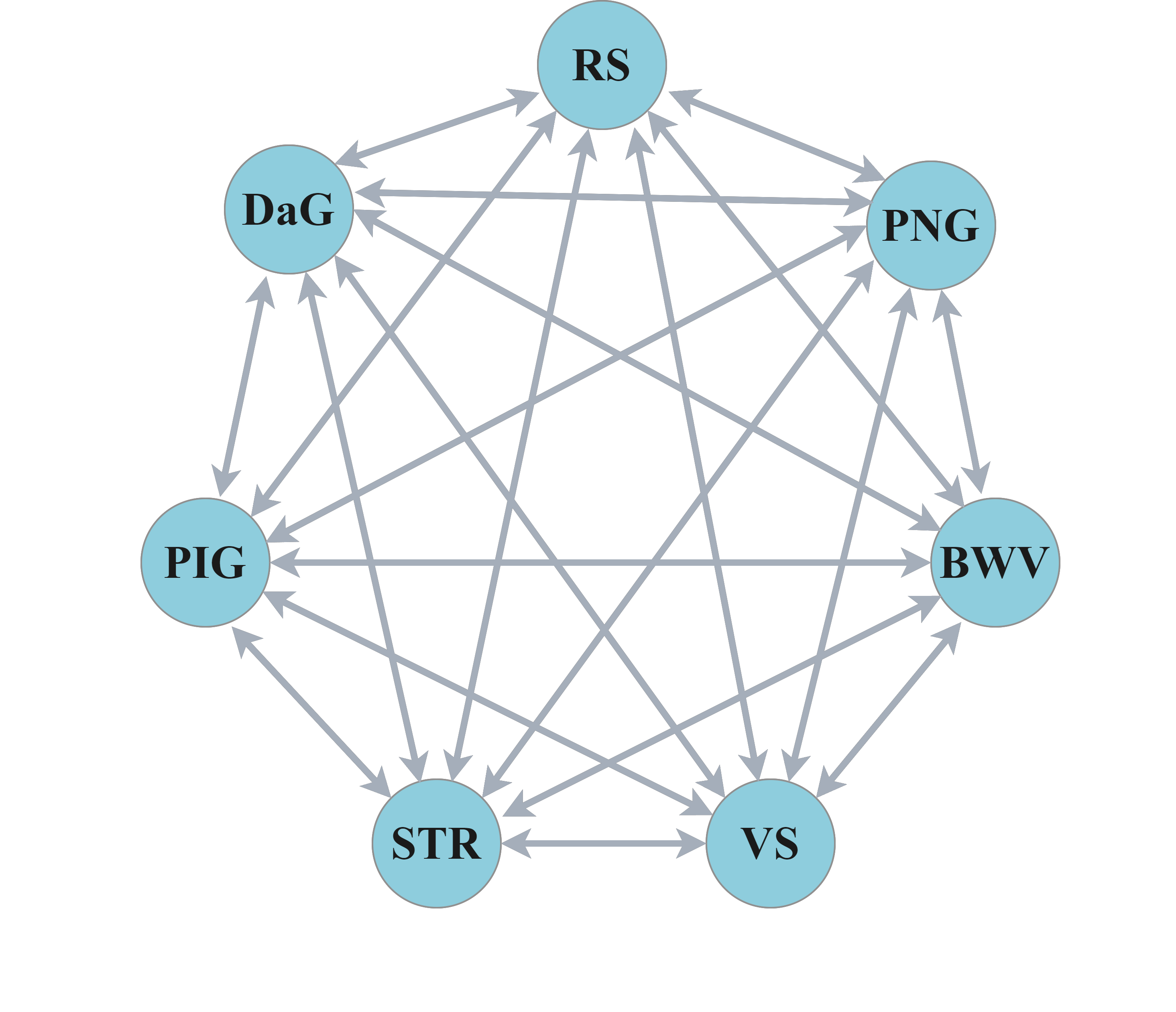
(b)

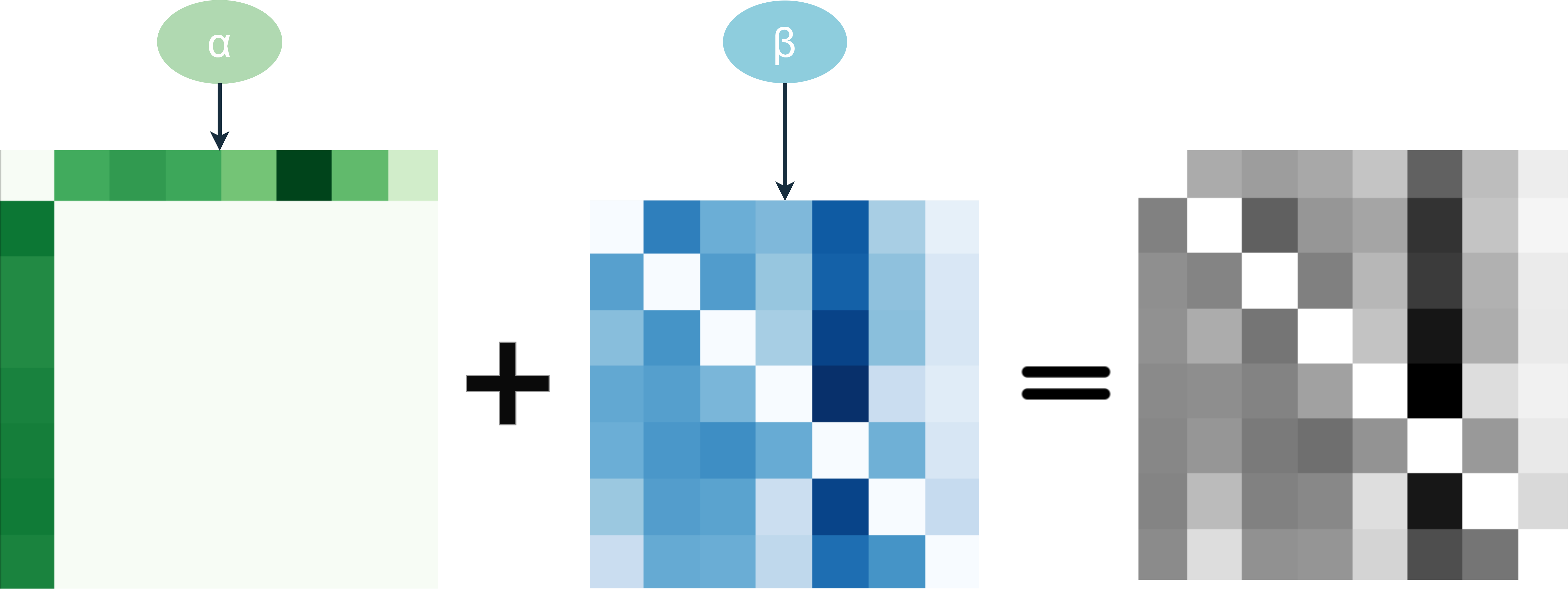
(c)

Figure 4: The illustration depicts the principles of both internal and external connectivity. The green nodes and matrix represent external connections between the seven attributes and melanoma, while the blue nodes and matrix represent internal connections among the seven attributes themselves. The gray matrix represents the final matrix obtained by the weighted fusion of the two.

2.2.3 Adaptive Receptive Field Proximity (ARFP)

When working with a weighted directed graph, the challenge initially lies in the absence of directed information along long paths, which results in insufficient global information and unbalanced receptive fields. Inspired by the digraph inception convolutional networks [29], we utilized the adjustable parameter $k$ to generate $k^{th}$-order proximity based on the information of both the meeting path and diffusion path. This approach enables the simultaneous extraction of direct and indirect connectivity information to the target and neighboring nodes, in contrast to relying solely on first- and second-order proximity. Given a graph $\mathcal{G}=(\mathcal{V},\mathcal{E})$, for $k\geq 2$, there exists a node $e\in\mathcal{V}$, the meeting path and diffusion path are defined as:

$$\left\{\begin{aligned} \mathcal{M}_{p,q}^{(k)}&=v_{p}\underbrace{\rightarrow\cdots\rightarrow}_{k-1\text{ edges }}v_{e}\underbrace{\leftarrow\cdots\leftarrow}_{k-1\text{ edges }}v_{q},\\ \mathcal{D}_{p,q}^{(k)}&=v_{p}\underbrace{\leftarrow\cdots\leftarrow}_{k-1\text{ edges }}v_{e}\underbrace{\rightarrow\cdots\rightarrow}_{k-1\text{ edges }}v_{q}.\end{aligned}\right.$$ (4)

where $\mathcal{M}_{p,q}^{(k)}$ and $\mathcal{D}_{p,q}^{(k)}$ represent the meeting path and diffusion path between nodes $p$ and $q$$(p,q\in\mathcal{V})$. If both $\mathcal{M}_{p,q}{}^{(k)}$ and $\mathcal{D}_{p,q}{}^{(k)}$ exist between nodes $p$ and $q$, then we consider them to be at the $k^{\text{th}}$-order proximity level, with $v_{e}$ being their $k^{\text{th}}$-order common neighbor. It is worth noting that a node has $0^{\text{th}}$-order proximity with itself and $1^{\text{st}}$-order proximity with its directly connected neighbors.

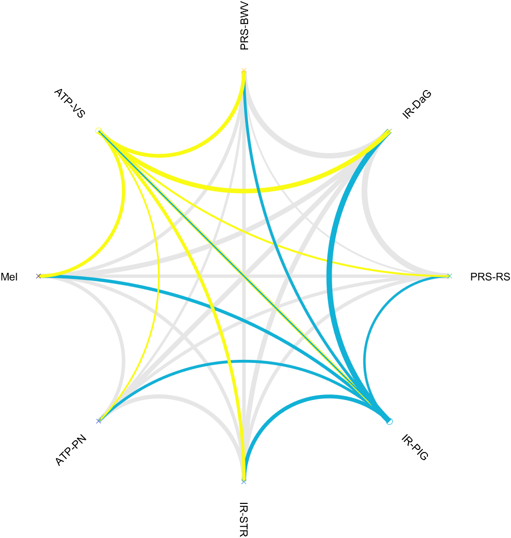
(a)

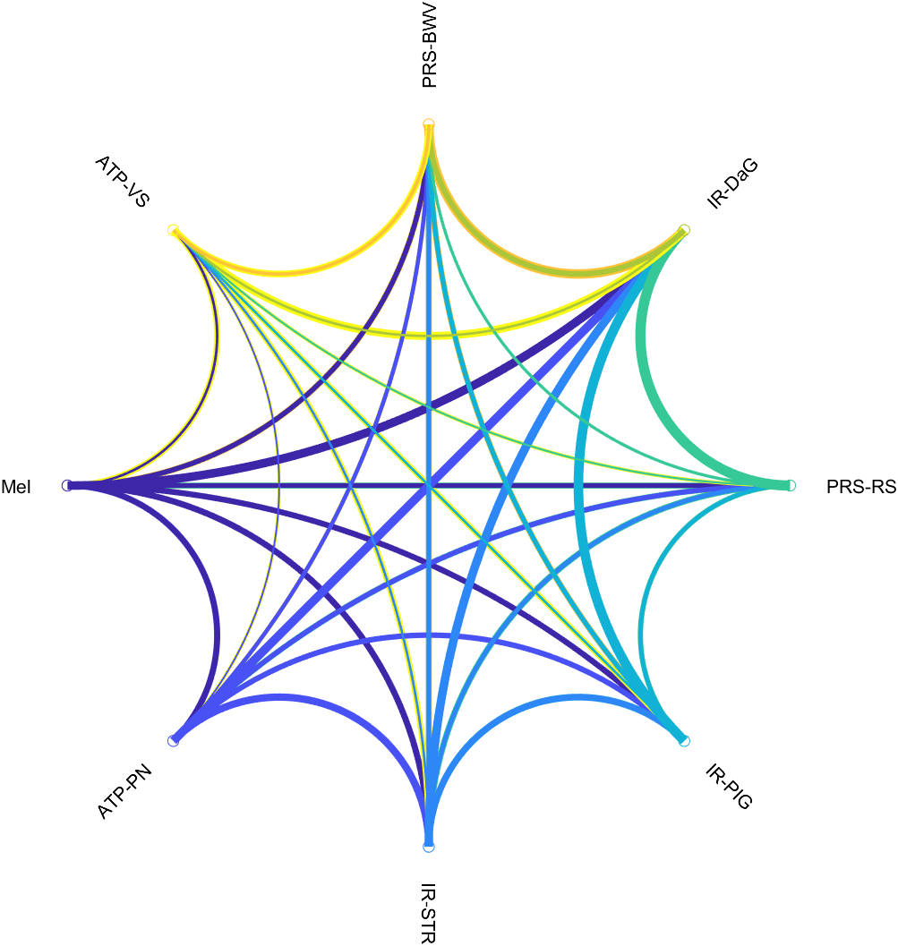
(b)

Figure 5: The plot illustrates the weighted connections in the training set of the EDRA dataset. while (a) focuses on a specific pair, ATP-VS and IR-PIG. Yellow lines represent connections from ATP-VS to the other nodes, while cyan lines represent connections from IR-PIG. Variations in line thickness highlight differences in directed weights between the nodes. Figure (b) displays the overall connectivity map among all eight nodes.

Using the 7PCL directed weighted graph and the $k^{\text{th}}$-order proximity, the 7PCL $k^{\text{th}}$-order proximity matrix founded on the conventional spectral-based GCN method is denoted as:

where ${{A}}$ represents the adjacency matrix of the directed weighted graph ${\mathcal{G}}$, and ${{D}}$ represents the corresponding diagonalized degree matrix. The matrix intersection operation $\text{intersect}(\cdot)$ creates a new matrix with the element-wise intersection of both meeting and diffusion paths. This operation aims to symmetrize the $k^{th}$-order proximity matrix ${P}^{(k)}$ to fit the structure of spectral-based GCN. Here, the value of parameter $k$ represents the distance between two similar nodes, which determines the size of the receptive fields. By adjusting the value of parameter $k$, users can observe and select the optimal receptive field with scalable capabilities.

Based on the $k^{th}$-order proximity matrix, the multi-scale digraph is then defined as:

where ${Z}^{(k)}$ represents the convolved output with dimensions $\mathbb{R}^{n\times d}$. ${X}$ denotes the node feature matrix with dimensions $\mathbb{R}^{n\times c}$. ${W}^{(k)}$ refers to the weight matrix, which is diagonalized from ${P}^{(k)}$, and ${\Theta}^{(k)}$, with dimensions $\mathbb{R}^{c\times d}$, is a trainable weight matrix. It’s noteworthy that when $k=1$, ${Z}^{(1)}$ is computed through digraph convolution using ${P}^{(1)}$ as defined in Eq. 5, and $\boldsymbol{\Pi}^{(1)}$ represents the corresponding approximate diagonalized eigenvector associated with ${P}^{(1)}$.

Table 1: Classification Performance (AUC, Prec, Sens, and Spec) of the Proposed Method Compared with the State-of-the-Art Methods, Evaluated on the EDRA Dataset

	Method	DIAG MEL	PN ATP	STR IR	PIG IR	RS PRS	DaG IR	BWV PRS	VS IR	Avg
AUC	Inception-combined [6]	86.3	79.9	78.9	79.0	82.9	79.9	89.2	76.1	81.5
	EmbeddingNet[30]	82.5	74.5	77.7	77.9	71.3	78.5	84.8	76.9	78.0
	TripleNet [31]	81.2	73.8	76.3	77.6	76.8	76.0	85.1	79.9	78.3
	Constrained-CC [23]	83.4	76.2	81.8	82.6	78.4	81.1	90.5	78.6	81.6
	HcCNN [20]	85.6	78.3	77.6	81.3	81.9	82.6	89.8	82.7	82.5
	GRM-DC [24]	87.6	87.5	81.2	83.6	79.0	83.1	90.8	75.4	83.5
	Ours	89.1	84.9	79.7	83.8	87.1	81.3	92.1	81.9	85.0
Prec	Inception-combined [6]	65.3	61.6	52.7	57.8	56.5	70.5	63.0	30.8	57.3
	EmbeddingNet [30]	68.3	52.5	58.5	61.5	76.8	70.8	89.5	36.8	64.4
	TripleNet [31]	61.8	59.6	61.7	54.7	77.7	65.7	90.6	64.3	67.0
	Constrained-CC [23]	54.4	66.1	62.8	43.0	76.1	77.8	67.4	75.7	65.4
	HcCNN [20]	62.8	62.3	52.4	65.1	81.6	69.6	91.9	50.0	67.0
	GRM-DC [24]	65.6	48.4	50.4	82.3	73.5	74.9	67.4	100	70.3
	Ours	77.7	65.8	57.1	74.5	77.6	75.7	75.0	37.1	67.6
Sens	Inception-combined [6]	61.4	48.4	51.1	59.7	66.0	62.1	77.3	13.3	54.9
	EmbeddingNet [30]	40.6	33.3	51.1	60.5	96.2	64.4	96.3	23.3	58.2
	TripleNet [31]	46.5	33.3	39.4	61.3	97.9	67.2	90.0	30.0	58.2
	Constrained-CC [23]	65.3	39.8	52.1	58.5	40.6	63.8	73.3	30.0	52.9
	HcCNN [20]	58.4	40.9	35.1	55.7	95.2	80.2	92.2	20.0	59.7
	GRM-DC [24]	59.0	77.5	67.0	39.2	21.9	70.1	69.9	3.6	51.0
	Ours	50.0	51.6	46.8	58.9	55.7	65.0	72.0	43.3	55.4
Spec	Inception-combined [6]	88.8	90.7	85.7	80.1	81.3	78.9	89.4	97.5	86.6
	EmbeddingNet [30]	93.5	90.7	88.7	82.7	20.8	78.4	52.0	96.7	75.4
	TripleNet [31]	90.1	93.0	92.4	76.8	23.6	71.6	60.0	98.6	75.8
	Constrained-CC [23]	81.6	93.7	90.4	75.7	95.6	85.3	91.6	99.2	89.1
	HcCNN [20]	88.1	92.4	90.0	86.3	41.5	71.6	65.3	98.4	79.2
	GRM-DC [24]	89.5	79.0	80.3	95.8	96.8	78.8	91.0	100	88.9
	Ours	95.5	91.7	89.0	90.7	94.1	83.0	94.3	94.0	91.5

2.3 Gradient Diagnostics with Data-Driven Weighting (GD-DDW)

As previously discussed, the deep features extracted from fused imaging modalities and the directed mutual connection matrix are collectively referred to as $X$ for subsequent diagnostic procedures. In this section, we present the GD-DDW method, designed to emulate the diagnostic approach employed by dermatologists using the 7-point checklist algorithm in clinical practice. Specifically, the GD-DDW method utilizes representative features corresponding to various attributes to make initial predictions, which are then used to diagnose melanoma.

In this module, we first establish a parallel multi-label classifier designed to address the classification of seven attributes on the checklist. As $X$ is the input, $y_{{\textrm{7p}}_{j}}=[y_{{\textrm{7p}}_{1}},y_{{\textrm{7p}}_{2}},...,y_{{\textrm{7p}}_{7}}]\in\{0,1\}^{7}$ is denoted as the ground truth of all seven attributes in the format of a binary indicator vector. In the proposed method, the focal loss function [32] was employed with the objective of enhancing the performance on the dataset that exhibiting a serious imbalance.

The focal loss function for each label can be defined as:

$$L_{{\textrm{7p}}_{j}}=-\mu_{j}(1-\hat{y}_{{\textrm{7p}}_{j}})^{\tau}\log(\hat{y}_{{\textrm{7p}}_{j}})$$ (7)

where $\hat{y}_{{\textrm{7p}}_{j}}$ represents the predicted probability of the positive class, $\mu_{j}$ is a balancing parameter, and $\tau$ is the focusing parameter. The total focal loss $L_{\textrm{7p}}$ for all seven attributes can be formulated as:

$$L_{\textrm{7p}}=\sum_{j=1}^{7}L_{{\textrm{7p}}_{j}}$$ (8)

Next, the prediction scores obtained for each label are utilized as inputs for the subsequent step. In this stage, a weighted sum function and a sigmoid activation function are applied to perform classification for the diagnosis of melanoma.

Let $w=[w_{1},w_{2},...,w_{j}]$ represent the learned weights module obtained from the attributes. In this module, the predicted probability of melanoma $\hat{y}_{\textrm{m}}$ is computed as:

$$\hat{y}_{\textrm{m}}=\sigma\left(\frac{1}{\sum_{j=1}^{7}w_{j}}\sum_{i=j}^{7}w_{j}\hat{y}_{{\textrm{7p}}_{j}}\right)$$ (9)

where $\sigma(\cdot)$ denotes the sigmoid activation function and the rescaling factor $\frac{1}{\sum_{j=1}^{7}w_{j}}$ ensures that the output is appropriately scaled to the range $[0,1]$.

The overall loss $L$ is then computed as the sum of $L_{\textrm{7p}}$ and $L_{\textrm{mel}}$:

$$L={L_{\textrm{7p}}}+{\lambda L_{\textrm{mel}}}$$ (10)

where $\lambda$ is the weighting parameter that adjusting the contributions of the two losses, specifically, making sure the loss values are in the same order of magnitude.

3 Experiments

3.1 Materials

In this study, we utilized the EDRA public dataset as the major material, purposefully curated for 7PCL studies and annotated by Kawahara et al [6]. This dataset comprises paired dermoscopic and clinical images sourced from 1011 patients, each image has a maximum resolution of 768 by 512 pixels. Notably, nine patients lacked clinical images, which were substituted with corresponding dermoscopic ones. Throughout our study, we strictly adhered to the dataset’s official specifications, which stipulated a total of 413 training, 203 validation, and 395 test images. Concerning the labels, the 7PCL attributes were incorporated into the analysis, following the official categorization. Notably, only the melanoma category was retained from the original disease categorization (DIAG). To verify the generalizability of our proposed method, we also used two publicly available datasets, ISIC 2017 and ISIC 2018 [18], which also have multiple attributes. The visual attributes contained in ISIC 2017 include milia-like cysts, negative network, pigment network, and streaks. A total of 2000 training, 150 validation, and 600 test images. ISIC 2018 adds an additional attribute, globules, to the 2017 version and adds a portion of the data to make the data distribution adjusted to 2594 training, 100 validation, and 1000 test images.

Table 2: Comparative Ablation Study of Key Modules in Our Proposed Method, Evaluated on the EDRA Dataset

Baseline (Clinical) Baseline (Derm) Derm & Clinical +IEDWG +ARFP +GD-DDW Ours DIAG MEL 75.6 78.2 77.8 83.5 86.5 83.2 89.1 PN TYP 71.7 75.8 79.4 84.2 85.5 81.5 84.9 ATP 69.5 66.9 68.5 83.9 82.5 77.2 80.2 STR REG 79.2 84.2 82.6 87.5 86.7 83.2 83.5 IR 58.5 67.9 71.6 79.4 77.2 75.3 79.7 PIG REG 66.7 67.8 71.3 71.0 70.2 71.4 82.3 IR 68.1 72.0 76.3 81.8 81.9 82.2 83.8 RS PRS 58.4 72.9 71.9 81.0 83.8 79.4 87.1 DaG REG 69.6 67.7 68.5 79.0 78.0 75.5 80.9 IR 67.1 71.3 70.4 81.0 80.3 79.5 81.3 BWV PRS 79.6 83.6 83.9 94.3 93.8 91.2 92.1 VS REG 71.5 75.6 79.1 82.8 83.9 84.9 86.1 IR 66.4 64.3 72.0 77.7 75.8 75.2 81.9 Avg 69.4 72.9 74.9 82.1 82.0 80.0 84.1

3.2 Implementation Details

In our study, we ensured the integrity of our results by employing consistent data processing methods and adhering to uniform model training protocols across various ablation comparison experiments. Our chosen deep learning model framework is ResNet-50, leveraging parameters pretrained on ImageNet, a common practice in other related works. The entire architecture is meticulously fine-tuned end-to-end, utilizing the Adam optimizer [33] with a concurrent learning rate set to 0.00001. We predefined the number of epochs for pretraining to 150, with an early-stopping mechanism in place. If the model’s performance on the validation set fails to improve over 50 consecutive epochs, the training process halts, and the best-performing model is saved. The loss functions utilized are based on focal loss to circumvent the result bias that may arise from imbalanced data. The hyperparameters for the different stages outlined in the methodology were selected based on insights gained from the training process and represent approximate ranges.

The initial stage of the process is the pre-processing of the images. To maintain consistency and minimize the impact of variable image formats, we eliminate the black edges from the images and resize them to 224 by 224 pixels, aligning with the requirements of the ResNet-50 backbone.

In the CD-MFM section, features from different channels undergo two stages of fusion using weighted averaging. Initially, a fusion process occurs between clinical and dermoscopy images, followed by a second fusion stage after incorporating topological relations learned by the graph network. The parameter $\delta$ in Eq. 1, which corresponds to the weight of clinical images, is set to 0.4, reflecting the dominance of dermoscopy in providing features related to 7PCL. Additionally, the parameters $\gamma$ series in Eq. 3 are configured to ${1}/{3}$ to mitigate potential biases stemming from assigning varying weights to the same feature across multiple instances.

In constructing the graph network, we consider only a subset of the possible connections between nodes due to the directionality of the multistep connections. Based on the average number of co-existing labels in the training set and the avoidance of isolated points, the connections are ordered according to the edge weights, ensuring that each node has at least one and no more than three edges. The order of connection $k$ is set to 3 due to the natural limitation of the number of nodes in 7PCL.

In the final diagnostic phase, the parameter $\lambda$, utilized in the global optimization of the loss function in Eq. 10, is set to 1, given that both loss values are of a comparable magnitude. All experiments were conducted on one NVIDIA Tesla V100 GPU card (32 GB memory) at the UBC ARC Sockeye using the PyTorch platform. The duration of each training cycle is approximately one hour. Our code is publicly available at https://github.com/Ryan315/7PGD.

3.3 Evaluation Settings

The study employed commonly used performance metrics such as the area under the receiver operating characteristic curve (AUC), sensitivity (Sens), specificity (Spec), and precision (Prec). To showcase the advantages of our method, we analyzed the results from various perspectives.

Initially, our method was compared with the state-of-the-art (SOTA) methods that utilized the same dataset and addressed the same task. These methods included GRM-DC [24], which considered intermodal and intercategory connections; 7PCL-Contrained-CC [23], considering the mutual connections between attributes; HcCNN, focusing on multi-channel modal fusion [20]; TripleNet, incorporating knowledge distillation transfer [31]; and the EmbeddingNet work proposed by Yap et al [30]. Specifically, we used the Inception models from the deep learning work of Kawahara et al. [6] as a baseline for comparison, as they originally published the data and proposed the first multi-modal, multi-label deep learning fusion method.

Next, ablation experiments were conducted to validate and analyze the role of crucial modules proposed in our method. Firstly, we verified the role of multimodal fusion CD-MFM by comparing unimodal and multimodal modalities. Secondly, the directed topology between features and diagnostics IEDWG, and the adjustable multi-order link ARFP used in graph network learning, were considered. Thirdly, our gradient-based prediction structure, GD-DDW, was employed for comparison with commonly used parallel prediction structures.

Then, as the proposed method draws inspiration from clinical algorithms in diagnosing real diseases, a comparison with clinical algorithms was also necessary. The prediction results of all attributes obtained in the first layer of the GD-DDW structure were utilized. Following the rule of summing the assigned scores in the clinic, different thresholds from 1 to 7 for the diagnostic scores were set to diagnose melanoma. This was then compared with the proposed method.

To validate the proposed method, we conducted comparative experiments on two additional publicly available datasets, ISIC 2017&2018. While the lack of information regarding the diagnosis precludes an evaluation of the impact of GD-DDW, the directed multi-order relationships between the attributes can still be validated.

Table 3: Comparison of Weights Value between Proposed Method and Traditional Algorithm.

	PN ATP	STR IR	PIG IR	RS PRS	DaG IR	BWV PRS	VS IR
Traditional	2	1	1	1	1	2	2
Proposed	1.47	0.95	0.93	0.92	0.97	1.42	1.35

Table 4: Performance (AUC) of Proposed Method on ISIC Datasets.

Dataset	Attributes	Baseline (ResNet-50)	GRM-DC [24]	CKTG (Proposed)
ISIC2017	Milia-like cysts	63.2	68.3	66.3
	Negative network	77.9	84.1	86.5
	Pigment network	87.3	87.4	89.6
	Streaks	96.2	93.9	94.1
	Avg	81.2	83.4	84.1
ISIC2018	Globules	68.2	77.1	79.3
	Milia-like cysts	60.1	68.8	66.7
	Negative network	82.3	87.3	87.9
	Pigment network	87.8	86.4	88.0
	Streaks	84.3	88.7	89.4
	Avg	76.5	81.7	82.3

4 Results

4.1 Comparison to State-of-the-Art Methods

Table 1 presented a comprehensive comparison of the classification performance between the proposed method and several state-of-the-art methods on the EDRA dataset. It demonstrated our method surpassed other SOTA methods with an average AUC of 85.0%. Notably, five out of the eight labels, specifically including melanoma, achieved the highest diagnostic results. Moreover, it was noteworthy that GRM-DC, which was also based on graph convolutional networks, was observed to be the methodology achieving the optimal AUC for the remaining two of three labels. This finding reinforced the notion that the interactions between attributes in 7PCL could not only aid in detecting melanoma but also offer insights for detecting each attribute.

As for the other three metrics, our method also demonstrated strong performance in precision (67.6%), particularly excelling in Mel (77.7%). The sensitivity of our method is 55.4%, particularly for VS, which represents an improvement of over 13% compared to other methods. As VS represents the most unbalanced attribute in this dataset (with only 71 positive subjects out of 1011), the resulting enhancement of this attribute highlights the significance of the interactions between the attributes learned by our approach. Additionally, it achieved the highest specificity (91.5%), excelling in Mel (95.5%) and BWV (94.3%).

4.2 Ablation Studies

Table 2 presented the results of the ablation experiments conducted on the various modules. The first comparison was between unimodality and multimodality. Consistent with previous related studies, the results showed that dermoscopy and clinical imaging fusion generally outperformed unimodality. Additionally, dermoscopy performed better than clinical images with 3% improvement, which was reasonable given that dermoscopy naturally provided more detailed features, especially in the context of 7PCL.

Regarding the impact of different modules on the results, both IEDWG and ARFD contributed to an average AUC improvement of 8%. Particularly, ARFD showed the highest improvement in melanoma’s results, increasing from 77.8% to 86.5%. This underscores the effectiveness of multi-order relationships between attributes in providing diagnostic information. Additionally, the gradient diagnostic structure, designed to mimic clinical diagnostic approaches, enhanced the average AUC by 5%. The integration of these three modules collectively resulted in a notable enhancement in model efficacy, as evidenced by the average AUC reaching 84.1%.

4.3 Comparison to Traditional 7PCL Algorithm

As shown in Table 3, the traditional algorithm employs approximate categorization based on multivariate analysis [34], assigning weights of 2 or 1 to major and minor attributes, respectively. In contrast, the method proposed in this study provides more precise weights, ranging from 1.3 to 1.5 for major attributes and from 0.9 to 1 for minor attributes, based on predicted scores for each category. Fig. 6 illustrates the discrepancy between the proposed method and the traditional 7PCL algorithm, based on identical forecasting outcomes for each attribute. The integration of predicted scores and data-driven weighting modules significantly enhances the prediction of melanoma. The predicted AUC improves from 72% to 89%, representing a substantial increase of 17%. Additionally, the ROC curve of the proposed method provides more accurate information regarding paired specificity and sensitivity, assisting dermatologists in more effective selection and analysis. While traditional methods offer initial guidance concisely, our method provides more detailed information, leveraging increasing computational resources. Moreover, the proposed method offers greater flexibility in setting thresholds and can be dynamically adjusted when the dataset changes, facilitating a more accurate determination of whether the detected lesion requires further biopsy treatment.

4.4 Generalizability Analysis on the ISIC Datasets

As illustrated in Table 4, we have predicted and compared the attributes present in the ISIC 2017 and 2018 datasets with the baseline utilized and the currently relevant SOTA, respectively. It is notable that our average AUC is the highest on both datasets, and specifically for each attribute, our proposed method attains the highest results in six out of nine attributes. This demonstrates that the proposed method is capable of effectively extracting the interactions between attributes, thereby enhancing the model’s predictive capability.

5 Discussion

In this study, a novel method to melanoma diagnosis was proposed, integrating clinical empirical knowledge, diagnostic procedures, and graph convolutional networks. Specifically, an appropriate topological graph structure was established by improving the causal learning of attributes associated with melanoma. Computational logic from clinical algorithms was borrowed to enhance explanatory power and clinical acceptance by improving the strong correlation between results and imaging datasets. Moreover, certain elements identified during this study warranted further discussion.

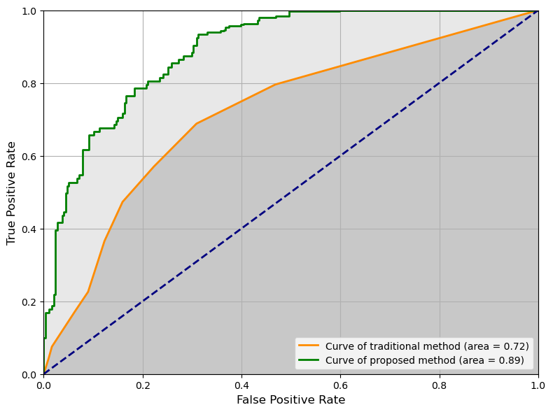
Figure 6: The ROC comparison graph illustrates the performance contrast between the proposed method and the traditional 7PCL algorithm.

Table 5: Comparison of One-Hot and GloVe.

	Semantic information	Training time		AUC
		Encoding	Total	Mel	Attributes
One-Hot	$\times$	3s	34 mins	86.8	81.1
GloVe	$\checkmark$	15s	45 mins	89.1	83.7

The results demonstrated the significance of the multi-order node associations introduced by ARFP as topological information, enhancing melanoma detection performance. In preliminary experiments, it was observed that the model’s performance improved as the order $k$ increased from 1 to 3. However, the results plateaued at order $k=4$. Upon closer examination, it was found that as the order $k$ increased, the number of links decreased sharply due to the limited number of nodes (7), resulting in the loss of useful information. Consequently, selecting the optimal order for this work was deemed paramount. Furthermore, the incorporation of additional, more informative labels may potentially enhance the overall outcome.

Additionally, current studies on graph networks related to melanoma detection have primarily focused on link information between nodes. However, for the first time, the semantic information contained in the category names of the nodes themselves was considered. As shown in Table 5, comparison data of predicted knots at the end of data processing time were retained in the study. It was observed that the semantic information of the nodes themselves, while increasing the total time for extraction and processing, resulted in a positive improvement in comparison. Indeed, numerous additional coding methods could be explored in future work.

In presenting the main results of this paper, we used the widely adopted ResNet-50 model to enhance the persuasiveness of our findings. Actually, in the preliminary studies, we experimented with various deep learning architectures, including EfficientNetV2-M, InceptionV3, and MobileNetV2. The results obtained from these models exhibit similar trends and comparisons to those of ResNet-50. The AUC values for melanoma (Mel) across these architectures range from 81.5% to 88.2%. The predictive capacity of our proposed framework may be further enhanced through the utilisation of more sophisticated feature extraction or fusion methodologies, such as the vision transformer (ViT) based models.

6 Conclusion

This study proposes an AI-enhanced 7PCL for melanoma detection using a unique topology enriched with clinical insights, simulating dermatologists’ diagnostic behavior. By considering directed multi-order relationships and a gradient prediction structure, our method provides weight measures for each attribute. This helps dermatologists intuitively analyze attributes, enhancing interpretability in clinical scenarios and improving detection performance and acceptance.

References

- [1] Jacques Ferlay ME, Rebecca L Siegel, MD Isabelle Soerjomataram and DVM Ahmedin Jemal “Global cancer statistics 2022: GLOBOCAN estimates of incidence and mortality worldwide for 36 cancers in 185 countries”, 2024
- [2] Haley D Heibel, Leah Hooey and Clay J Cockerell “A review of noninvasive techniques for skin cancer detection in dermatology” In American journal of clinical dermatology 21.4 Springer, 2020, pp. 513–524
- [3] M Emre Celebi, Noel Codella and Allan Halpern “Dermoscopy image analysis: overview and future directions” In IEEE journal of biomedical and health informatics 23.2 IEEE, 2019, pp. 474–478
- [4] David Wen et al. “Characteristics of publicly available skin cancer image datasets: a systematic review” In The Lancet Digital Health 4.1 Elsevier, 2022, pp. e64–e74
- [5] Naheed R Abbasi et al. “Early diagnosis of cutaneous melanoma: revisiting the ABCD criteria” In Jama 292.22 American Medical Association, 2004, pp. 2771–2776
- [6] Jeremy Kawahara, Sara Daneshvar, Giuseppe Argenziano and Ghassan Hamarneh “Seven-point checklist and skin lesion classification using multitask multimodal neural nets” In IEEE journal of biomedical and health informatics 23.2 IEEE, 2018, pp. 538–546
- [7] Catarina Barata, M Emre Celebi and Jorge S Marques “Development of a clinically oriented system for melanoma diagnosis” In Pattern Recognition 69 Elsevier, 2017, pp. 270–285
- [8] M Emre Celebi et al. “A methodological approach to the classification of dermoscopy images” In Computerized Medical imaging and graphics 31.6 Elsevier, 2007, pp. 362–373
- [9] Gerald Schaefer, Bartosz Krawczyk, M Emre Celebi and Hitoshi Iyatomi “An ensemble classification approach for melanoma diagnosis” In Memetic Computing 6 Springer, 2014, pp. 233–240
- [10] Gabriella Fabbrocini et al. “Automatic diagnosis of melanoma based on the 7-point checklist” In Computer Vision Techniques for the Diagnosis of Skin Cancer Springer, 2014, pp. 71–107
- [11] Tarun Wadhawan et al. “Implementation of the 7-point checklist for melanoma detection on smart handheld devices” In 2011 annual international conference of the IEEE engineering in medicine and biology society, 2011, pp. 3180–3183 IEEE
- [12] Andre Esteva et al. “Dermatologist-level classification of skin cancer with deep neural networks” In nature 542.7639 Nature Publishing Group, 2017, pp. 115–118
- [13] Yuheng Wang et al. “Deep learning enhances polarization speckle for in vivo skin cancer detection” In Optics & Laser Technology 140 Elsevier, 2021, pp. 107006
- [14] Qaisar Abbas and M Emre Celebi “DermoDeep-A classification of melanoma-nevus skin lesions using multi-feature fusion of visual features and deep neural network” In Multimedia Tools and Applications 78.16 Springer, 2019, pp. 23559–23580
- [15] Catarina Barata, M Emre Celebi and Jorge S Marques “A survey of feature extraction in dermoscopy image analysis of skin cancer” In IEEE journal of biomedical and health informatics 23.3 IEEE, 2018, pp. 1096–1109
- [16] Kumar Abhishek, Jeremy Kawahara and Ghassan Hamarneh “Predicting the clinical management of skin lesions using deep learning” In Scientific reports 11.1 Nature Publishing Group UK London, 2021, pp. 7769
- [17] Catarina Barata et al. “A reinforcement learning model for AI-based decision support in skin cancer” In Nature Medicine Nature Publishing Group US New York, 2023, pp. 1–6
- [18] Noel CF Codella et al. “Skin lesion analysis toward melanoma detection: A challenge at the 2017 international symposium on biomedical imaging (isbi), hosted by the international skin imaging collaboration (isic)” In 2018 IEEE 15th international symposium on biomedical imaging (ISBI 2018), 2018, pp. 168–172 IEEE
- [19] Nayara Moura et al. “ABCD rule and pre-trained CNNs for melanoma diagnosis” In Multimedia Tools and Applications 78 Springer, 2019, pp. 6869–6888
- [20] Lei Bi, David Dagan Feng, Michael Fulham and Jinman Kim “Multi-label classification of multi-modality skin lesion via hyper-connected convolutional neural network” In Pattern Recognition 107 Elsevier, 2020, pp. 107502
- [21] Peng Tang et al. “FusionM4Net: A multi-stage multi-modal learning algorithm for multi-label skin lesion classification” In Medical Image Analysis 76 Elsevier, 2022, pp. 102307
- [22] Junyan Wu et al. “Learning differential diagnosis of skin conditions with co-occurrence supervision using graph convolutional networks” In Medical Image Computing and Computer Assisted Intervention–MICCAI 2020: 23rd International Conference, Lima, Peru, October 4–8, 2020, Proceedings, Part II 23, 2020, pp. 335–344 Springer
- [23] Yuheng Wang et al. “Incorporating clinical knowledge with constrained classifier chain into a multimodal deep network for melanoma detection” In Computers in Biology and Medicine 137 Elsevier, 2021, pp. 104812
- [24] Xiaohang Fu et al. “Graph-based intercategory and intermodality network for multilabel classification and melanoma diagnosis of skin lesions in dermoscopy and clinical images” In IEEE Transactions on Medical Imaging 41.11 IEEE, 2022, pp. 3266–3277
- [25] B De Pace et al. “Reinterpreting dermoscopic pigment network with reflectance confocal microscopy for identification of melanoma-specific features” In Journal of the European Academy of Dermatology and Venereology 32.6 Wiley Online Library, 2018, pp. 947–955
- [26] Riccardo Pampena et al. “Clinical and dermoscopic features associated with difficult-to-recognize variants of cutaneous melanoma: a systematic review” In JAMA dermatology 156.4 American Medical Association, 2020, pp. 430–439
- [27] Katherine Shi et al. “A retrospective cohort study of the diagnostic value of different subtypes of atypical pigment network on dermoscopy” In Journal of the American Academy of Dermatology 83.4 Elsevier, 2020, pp. 1028–1034
- [28] Jeffrey Pennington, Richard Socher and Christopher D Manning “Glove: Global vectors for word representation” In Proceedings of the 2014 conference on empirical methods in natural language processing (EMNLP), 2014, pp. 1532–1543
- [29] Zekun Tong et al. “Digraph inception convolutional networks” In Advances in neural information processing systems 33, 2020, pp. 17907–17918
- [30] Jordan Yap, William Yolland and Philipp Tschandl “Multimodal skin lesion classification using deep learning” In Experimental dermatology 27.11 Wiley Online Library, 2018, pp. 1261–1267
- [31] Zongyuan Ge et al. “Skin disease recognition using deep saliency features and multimodal learning of dermoscopy and clinical images” In Medical Image Computing and Computer Assisted Intervention- MICCAI 2017: 20th International Conference, Quebec City, QC, Canada, September 11-13, 2017, Proceedings, Part III 20, 2017, pp. 250–258 Springer
- [32] Tsung-Yi Lin et al. “Focal loss for dense object detection” In Proceedings of the IEEE international conference on computer vision, 2017, pp. 2980–2988
- [33] Zijun Zhang “Improved adam optimizer for deep neural networks” In 2018 IEEE/ACM 26th international symposium on quality of service (IWQoS), 2018, pp. 1–2 Ieee
- [34] Giuseppe Argenziano et al. “Epiluminescence microscopy for the diagnosis of doubtful melanocytic skin lesions: comparison of the ABCD rule of dermatoscopy and a new 7-point checklist based on pattern analysis” In Archives of dermatology 134.12 American Medical Association, 1998, pp. 1563–1570