Accelerated Quantum Amplitude Estimation without QFT

Abstract

We put forward a Quantum Amplitude Estimation algorithm delivering superior performance (lower quantum computational complexity and faster classical computation parts) compared to the approaches available to-date. The algorithm does not relay on the Quantum Fourier Transform and its quantum computational complexity is of order $O(\frac{1}{\varepsilon})$ in terms of the target accuracy $\varepsilon>0$. The $O(\frac{1}{\varepsilon})$ bound on quantum computational complexity is also superior compared to those in the earlier approaches due to smaller constants. Moreover, a much tighter bound is obtained by means of computer-assisted estimates for the expected value of quantum computational complexity. The correctness of the algorithm and the $O(\frac{1}{\varepsilon})$ bound on quantum computational complexity are supported by precise proofs.

1 Introduction

Let $\mathbf{A}$ be a unitary operator representing a quantum circuit such that

$$\mathbf{A}\left|0\right\rangle_{w+1}=\sqrt{1-a}\left|\Psi_{0}\right\rangle_{w}\!\left|0\right\rangle+\sqrt{a}\left|\Psi_{1}\right\rangle_{w}\!\left|1\right\rangle$$ (1)

for some unknown $a\in[0,1]$, where $\left|\Psi_{0}\right\rangle_{w}$ and $\left|\Psi_{1}\right\rangle_{w}$ are normalised states of width $w$ (that is, $w$-qubit states). The goal of Quantum Amplitude Estimation (QAE) is to compute an estimate $\hat{a}$ of $a$ to within given accuracy $\varepsilon>0$ at a prescribed confidence level $1-\alpha\in\left(0,1\right)$, so that

$$\mathbb{P}\{|\hat{a}-a|\leq\varepsilon\}\geq 1-\alpha.$$ (2)

QAE is one of the fundamental procedures in quantum computing, and a building block for quantum algorithms in diverse areas such as machine learning, chemistry, or finance. In particular, QAE gives rise to quadratic quantum speedup in Monte Carlo estimation.

Brassard et al. [Bra2002] were the first to establish a QAE procedure by combining ideas from the Grover and Shor quantum algorithms. The approach of [Bra2002], when adapted to an operator $\mathbf{A}$ of the form (1), was to consider the operator

$$\mathbf{Q}=\mathbf{AS}_{0}\mathbf{A}^{\dagger}\mathbf{S}_{\Psi_{0}},$$

where $\mathbf{S}_{0}=\mathbf{I}_{w+1}-2\left|0\right\rangle_{w+1}\!\left\langle 0\right|_{w+1}$ and $\mathbf{S}_{\Psi_{0}}=\mathbf{I}_{w}\otimes\left(\mathbf{I}-2\left|0\right\rangle\!\left\langle 0\right|\right)$, and apply to the state $\mathbf{A}\left|0\right\rangle_{w+1}$ the operators $\mathbf{Q}^{2^{0}},\mathbf{Q}^{2^{1}},\ldots,\mathbf{Q}^{2^{j-1}}$ controlled by $j$ ancillary qubits, sandwiched between the Quantum Fourier Transform (QFT) and the inverse QFT acting on the ancillary qubits. The quantum computational complexity of the QAE algorithm in [Bra2002], understood as the number of applications of $\mathbf{Q}$, is of order $O(\frac{1}{\varepsilon})$. However, the cost in terms of quantum computing resources is considerable due to the use of QFT and controlled gates $\mathbf{Q}^{2^{0}},\mathbf{Q}^{2^{1}},\ldots,\mathbf{Q}^{2^{j-1}}$. It is important to seek more efficient and less costly QAE procedures that lend themselves to implementation on near-term quantum computers, while matching the computational complexity of order $O(\frac{1}{\varepsilon})$.

Suzuki et al. [Suz2020] put forward a version of QAE which does not rely on QFT or controlled gates $\mathbf{Q}^{2^{0}},\mathbf{Q}^{2^{1}},\ldots,\mathbf{Q}^{2^{j-1}}$, reducing the circuit width and depth as compared to [Bra2002]. After measuring the rightmost qubit in the states $\mathbf{Q}^{2^{0}}\mathbf{A}\left|0\right\rangle_{w+1},\mathbf{Q}^{2^{1}}\mathbf{A}\left|0\right\rangle_{w+1},\ldots,\mathbf{Q}^{2^{j-1}}\mathbf{A}\left|0\right\rangle_{w+1}$, the authors of [Suz2020] applied maximum likelihood estimation to obtain an approximation of $a$. They justified this procedure by heuristic considerations and demonstrated empirically that the number of applications of $\mathbf{Q}$ needed to achieve accuracy $\varepsilon$ appears to scale roughly as $O\left(\frac{1}{\varepsilon}\right)$, but provided no rigorous proof to support this conjecture.

Aaranson and Rall [Aar2020] proposed a QAE algorithm without QFT or controlled gates $\mathbf{Q}^{k}$, proven to achieve the same quantum computational complexity of order $O(\frac{1}{\varepsilon})$ as in [Bra2002], but with large constants making it ill-suited for implementation on near-term quantum computers. Near-term efficiency was considerably improved by Grinko et al. [Gri2021] at the expense of asymptotic computational complexity of the QAE algorithm, for which the authors obtained a bound of order $O(\frac{1}{\varepsilon}\log(\log\frac{1}{\varepsilon}))$. A different algorithm of this kind, also with query complexity of order $O(\frac{1}{\varepsilon}\log(\log\frac{1}{\varepsilon}))$, belongs to Nakaji [Nak2020]. Fukuzawa et al. [Fuk2023] proposed a modification of the algorithm in [Gri2021] with computational complexity of order $O(\frac{1}{\varepsilon})$ and constants competitive with those in [Gri2021] and [Nak2020].

Here we present another version of QAE, also related to that in [Gri2021], but with computational complexity of order $O(\frac{1}{\varepsilon})$ and even better constants in the asymptotic bound, and better performance than all the aforesaid approaches. In Algorithms 1 and 2 we present variants of QAE which do not utilize QFT or controlled gates $\mathbf{Q}^{k}$ either and accomplish these aims. Theorems 2 and 4 provide precise proofs of the correctness of the algorithms, that is, of achieving (2), with upper bounds on the number of applications of $\mathbf{Q}$ of order $O(\frac{1}{\varepsilon})$ and constants smaller than in the papers listed above. Indeed, our algorithms, and particularly Algorithm 2, reduce the number of applications of $\mathbf{Q}$ as compared to all previous work, including [Gri2021] and [Fuk2023]. This being so, our algorithms are well suited for near-term quantum computers. The classical computation parts of the algorithms are also more efficient compared, for example, to [IQAE] and [MIQAE].

We rely on the following well-known property of $\mathbf{Q}$ (see [Bra2002]):

$$\mathbf{Q}^{k}\mathbf{A}\left|0\right\rangle_{w+1}=\cos\left(\left(2k+1\right)\theta\right)\left|\Psi_{0}\right\rangle_{w}\!\left|0\right\rangle+\sin\left(\left(2k+1\right)\theta\right)\left|\Psi_{1}\right\rangle_{w}\!\left|1\right\rangle$$ (3)

for each $k=0,1,2,\ldots$ , where

$$\sin^{2}(\theta)=a\quad\text{with}\quad\theta\in\textstyle\left[0,\frac{\pi}{2}\right].$$

It means that a measurement of the rightmost qubit in (3) will produce $\left|1\right\rangle$ with probability $\sin^{2}\left(\left(2k+1\right)\theta\right)$. We write

$$n=\texttt{{QuantCirc}}(k,N)$$

for the number of times when outcome $\left|1\right\rangle$ is produced in $N$ runs of the circuit $\mathbf{Q}^{k}\mathbf{A}\left|0\right\rangle_{w+1}$ followed by a measurement of the rightmost qubit. Hence, $n$ can be regarded as the number of successful outcomes in $N$ i.i.d. Bernoulli trials with probability of success $\sin^{2}\left(\left(2k+1\right)\theta\right)$, and $\frac{n}{N}$ can be taken as an estimate for the probability of a successful outcome, that is, outcome $\left|1\right\rangle$.

Let

$$\sin^{2}((2k+1)\hat{\theta})=\frac{n}{N}$$ (4)

for some $\hat{\theta}\in\left[0,\frac{\pi}{2}\right]$, and let $E$ and $F$ be given by (43) and (45). These constants are such that if

$$|\sin^{2}((2k+1)\hat{\theta})-\sin^{2}((2k+1)\theta)|\leq 2E,$$

(which will be so with high probability if $N$ is large enough), then

$$|(2k+1)\hat{\theta}-(2k+1)\theta|\leq 2F,$$

as long as there is an integer $m$ such that both $(2k+1)\hat{\theta}$ and $(2k+1)\theta$ belong to the same interval $\left[m\frac{\pi}{2},(m+1)\frac{\pi}{2}\right]$. In that case we get $|\hat{\theta}-\theta|\leq\frac{2F}{2k+1}$, and taking $\hat{a}=\sin^{2}(\hat{\theta})$ as an estimate for $a=\sin^{2}(\theta)$, we obtain

$$|\hat{a}-a|=|\sin^{2}(\hat{\theta})-\sin^{2}(\theta)|\leq|\hat{\theta}-\theta|\leq\frac{2F}{2k+1}.$$

The accuracy $\frac{2F}{2k+1}$ of this estimate can be made as small as desired by taking a sufficiently large $k$. However, for this to work we need to know the value of $m$ such that $(2k+1)\theta$ belongs to $\left[m\frac{\pi}{2},(m+1)\frac{\pi}{2}\right]$, so that among all the solutions $\hat{\theta}$ of equation (4) we can select the one that belongs to the interval $\left[m\frac{\pi}{2},(m+1)\frac{\pi}{2}\right]$. But we do not know $\theta$ (because we do not know $a$), and will need to rely on Lemma 6 to keep track of $m$. We do this in a different and perhaps simpler manner than Grinko et al. [Gri2021] or Fukuzawa et al. [Fuk2023].

Where our approach differs significantly from [Gri2021] is in how we achieve computational complexity $O(\frac{1}{\varepsilon})$ rather than $O(\frac{1}{\varepsilon}\log(\log(\frac{1}{\varepsilon})))$. Instead of assigning the same fraction $\frac{\alpha}{T}$ of $\alpha$ to each round $i$ of the main loop in the algorithm in [Gri2021] (where $1-\alpha$ is the prescribed confidence level and $T$ is an upper bound on the number of rounds), we take $\alpha_{i}$ increasing with $i$ as defined by (10) or (25) in such a manner that the sum of the$~{}\alpha_{i}$’s over all the rounds $i$ does not exceed $\alpha$. This is similar to, but different from [Fuk2023], leading to better constants in the asymptotics for computational complexity and better performance for relevant input data ranges. For low values of $i$, that is, when the powers of the $\mathbf{Q}$ operator in the quantum circuit are also low, the lower values of $\alpha_{i}$ force more runs of the circuit. But fewer runs are needed as $i$ and $\alpha_{i}$ increase and the powers of $\mathbf{Q}$ become higher. This is what makes it possible to reduce the upper bound for the overall number of applications of $\mathbf{Q}$ from $O(\frac{1}{\varepsilon}\log(\log(\frac{1}{\varepsilon})))$ to $O(\frac{1}{\varepsilon})$ with tight constants, as demonstrated in Theorems 2 and 4. Moreover, in Remarks 3 and 5 we show that our choice of the $\alpha_{i}$ is optimal in a certain sense.

The above upper bounds on quantum computational complexity, which is a random variable, are worst-case estimates holding with probability greater than or equal to the prescribed confidence level $1-\alpha$. A more representative quantity is the expected value of quantum computational complexity, that is, the expected number of applications of $\mathbf{Q}$, for which we obtain a much tighter bound by means of computer-assisted estimates.

Notation 1

Throughout this paper we denote by $\left[x,y\right]$ the closed interval with end-points $x,y\in\mathbb{R}$, irrespective of whether $x\leq y$ or $y\leq x$.

2 Accelerated QAE algorithm

We begin with formulating a simple version of our algorithm; see Algorithm 1. We prove the correctness of this algorithm and obtain an upper bound for quantum computational complexity in Theorem 2.

Algorithm 1

1:$\varepsilon>0$ and $\alpha\in(0,1)$

2:$E:=\frac{1}{2}\left(\sin^{2}\left(\frac{3}{7}\frac{\pi}{2}\right)-\sin^{2}\left(\frac{1}{3}\frac{\pi}{2}\right)\right),\quad F:=\frac{1}{2}\arcsin\sqrt{2E}$

3:$C:=\frac{4}{6F+\pi}$

4:$i:=-1,\quad K_{0}:=1,\quad m_{0}:=0$

5:repeat

6:     $i:=i+1$

7:     $\alpha_{i}:=C\alpha\varepsilon K_{i},\quad N_{i}:=\left\lceil\frac{1}{2E^{2}}\ln\frac{2}{\alpha_{i}}\right\rceil$

8:     $n_{i}:=\texttt{{QuantCirc}}(\frac{K_{i}-1}{2},N_{i}),\quad\hat{A}_{i}:=\frac{n_{i}}{N_{i}}$

9:     compute $\hat{\theta}^{\flat}_{i}$ and $\hat{\theta}^{\sharp}_{i}$ such that

10:   $K_{i}\hat{\theta}^{\flat}_{i},K_{i}\hat{\theta}^{\sharp}_{i}\in\big{[}m_{i}\frac{\pi}{2},(m_{i}+1)\frac{\pi}{2}\big{]}$

11:   and $\sin^{2}(K_{i}\hat{\theta}^{\flat}_{i})=\max\{\hat{A}_{i}-E,0\}$

12:   and $\sin^{2}(K_{i}\hat{\theta}^{\sharp}_{i})=\min\{\hat{A}_{i}+E,1\}$

13:     find $L_{i}\in\{3,5,7\}$ and $m_{i+1}\in L_{i}m_{i}+\{0,\ldots,L_{i}-1\}$ such that

14:   $[L_{i}K_{i}\hat{\theta}^{\flat}_{i},L_{i}K_{i}\hat{\theta}^{\sharp}_{i}]\subset\big{[}m_{i+1}\frac{\pi}{2},(m_{i+1}+1)\frac{\pi}{2}\big{]}$

15:     $K_{i+1}:=L_{i}K_{i}$

16:until $|\hat{\theta}^{\sharp}_{i}-\hat{\theta}^{\flat}_{i}|\leq 2\varepsilon$

17:$I:=i$

18:return $\hat{a}:=\sin^{2}(\frac{1}{2}{}(\hat{\theta}^{\flat}_{I}+\hat{\theta}^{\sharp}_{I}))$

Theorem 2

Given an accuracy $\varepsilon>0$ and confidence level $1-\alpha\in(0,1)$, Algorithm 1 returns an estimate $\hat{a}$ of $a$ such that

$$\mathbb{P}\{\left|\hat{a}-a\right|\leq\varepsilon\}\geq 1-\alpha.$$ (5)

The algorithm involves at most

$$M <\frac{1}{\varepsilon}\left(\frac{1}{4E^{2}}\left(\frac{3}{2}F\ln\left(\frac{2}{C\alpha F}\right)+\frac{3}{4}F\ln\left(3\right)+\frac{\pi}{4}\ln\left(\frac{8}{C\alpha\pi}\right)\right)+\frac{3}{4}F+\frac{\pi}{8}\right)$$

$$\approx\frac{1}{\varepsilon}\left(85.637-55.674\ln\left(\alpha\right)\right)$$ (6)

applications of $\mathbf{Q}$, where the constants $E,F,C$ are given by (43), (45), (13). That is, the quantum computational complexity $M$ of the algorithm scales as $O(\frac{1}{\varepsilon})$.

Proof. Take an $a\in\left[0,1\right]$ and the angle $\theta\in\left[0,\frac{\pi}{2}\right]$ such that

$$a=\sin^{2}(\theta),$$

and for each $i=0,1,\ldots$ put

$$A_{i}=\sin^{2}(K_{i}\theta).$$

For the sake of this argument, suppose that the repeat loop in Algorithm 1 does not break when the condition $|\hat{\theta}_{i}^{\sharp}-\hat{\theta}_{i}^{\flat}|\leq 2\varepsilon$ is satisfied, but keeps running indefinitely. This defines $\alpha_{i},N_{i},n_{i},\hat{A}_{i},K_{i},\hat{\theta}_{i}^{\sharp},\hat{\theta}_{i}^{\sharp},L_{i},m_{i}$ for each $i=0,1,\ldots$ . Then, $I$ can be taken to be the smallest $i=0,1,\ldots$ satisfying the condition $|\hat{\theta}_{i}^{\sharp}-\hat{\theta}_{i}^{\flat}|\leq 2\varepsilon$.

We have

$$\hat{A}_{i}=\frac{n_{i}}{N_{i}},$$ (7)

where

$$n_{i}=\textstyle\texttt{{QuantCirc}}(\frac{K_{i}-1}{2},N_{i})$$ (8)

can be regarded as the number of successful outcomes in $N_{i}$ i.i.d. Bernoulli trials with probability of success $A_{i}$. Let

$$B=\textstyle\bigcap_{i=0}^{I}B_{i},$$

where, for each $i=0,1,\ldots\,$,

$$B_{i}=\{|\hat{A}_{i}-A_{i}|\leq E\}$$

with

$$N_{i}=\left\lceil\frac{1}{2E^{2}}\ln\frac{2}{\alpha_{i}}\right\rceil$$ (9)

and

$$\alpha_{i}=C\alpha\varepsilon K_{i}.$$ (10)

In these formulae $E$ and $F$ are given by (43) and (45), and $C$ by (13). By Hoeffding’s inequality [Hoeff] for $N_{i}$ i.i.d.  Benoulli trials applied to the probability of $B_{i}$ conditioned on the algorithm outcomes for rounds $0,1,\ldots,i-1$ of the repeat loop, we have

$$\mathbb{P}(B_{i}|B_{0}\cap\cdots\cap B_{i-1})\geq 1-2e^{-2N_{i}E^{2}}\geq 1-\alpha_{i}$$

for each $i=0,1,\ldots\,$.

Consider the situation when the outcome of Algorithm 1 is in $B$. Observe that

$$|K_{I-1}\hat{\theta}_{I-1}^{\sharp}-K_{I-1}\hat{\theta}_{I-1}^{\flat}|=2f(\hat{A}_{I-1},E)\leq 2f(E,E)\leq 2F$$

by the definitions and properties of $E,F,f$ (see Section 3) and the fact that $\sin^{2}(K_{I-1}\hat{\theta}_{I-1}^{\flat})=\max\{\hat{A}_{I-1}-E,0\}$, $\sin^{2}(K_{I-1}\hat{\theta}_{I-1}^{\sharp})=\min\{\hat{A}_{I-1}+E,1\}$, and $K_{I-1}\hat{\theta}_{I-1}^{\sharp},K_{I-1}\hat{\theta}_{I-1}^{\flat}\in\left[m_{I-1}\frac{\pi}{2},(m_{I-1}+1)\frac{\pi}{2}\right]$. We have $|\hat{\theta}_{I-1}^{\sharp}-\hat{\theta}_{I-1}^{\flat}|>2\varepsilon$ since $I$ is the smallest $i=0,1,\ldots$ satisfying the condition $|\hat{\theta}_{i}^{\sharp}-\hat{\theta}_{i}^{\flat}|\leq 2\varepsilon$. It follows that

$$K_{I-1}\leq\frac{2F}{|\hat{\theta}_{I-1}^{\sharp}-\hat{\theta}_{I-1}^{\flat}|}<\frac{F}{\varepsilon}.$$

Then, for each $i=0,1,\ldots,I-1$,

$$K_{i}\leq\frac{L_{I-2}}{3}\times\cdots\times\frac{L_{i}}{3}K_{i}=3^{-I+1+i}K_{I-1}<3^{-I+1+i}\frac{F}{\varepsilon}$$ (11)

since $L_{i},\ldots,L_{I-2}\in\left\{3,5,7\right\}$. For $i=I$, this inequality would read $K_{I}\leq\frac{3F}{\varepsilon}$, but this may not hold. However, there is a higher bound for $K_{I}$, namely,

$$K_{I}<\frac{\pi}{4\varepsilon}.$$ (12)

The last inequality holds because $|\hat{\theta}_{I-1}^{\sharp}-\hat{\theta}_{I-1}^{\sharp}|>2\varepsilon$ and $K_{I}\hat{\theta}_{I-1}^{\flat},K_{I}\hat{\theta}_{I-1}^{\sharp}\in\left[m_{I}\frac{\pi}{2},\left(m_{I}+1\right)\frac{\pi}{2}\right]$, which means that $|K_{I}\hat{\theta}_{I-1}^{\sharp}-K_{I}\hat{\theta}_{I-1}^{\flat}|\leq\frac{\pi}{2}$.

It follows that

$$\sum_{i=0}^{I}\alpha_{i} =C\alpha\varepsilon\sum_{i=0}^{I}K_{i}<C\alpha\bigg{(}\sum_{i=0}^{I-1}3^{-I+1+i}F+\frac{\pi}{4}\bigg{)}=C\alpha\bigg{(}\sum_{j=0}^{I-1}3^{-j}F+\frac{\pi}{4}\bigg{)}$$

$$<C\alpha\bigg{(}\sum_{j=0}^{\infty}3^{-j}F+\frac{\pi}{4}\bigg{)}=C\alpha\bigg{(}\frac{3}{2}F+\frac{\pi}{4}\bigg{)}=C\alpha\frac{6F+\pi}{4}=\alpha$$

when

$$C=\frac{4}{6F+\pi}\approx 0.93314.$$ (13)

Since the events $B_{0},B_{1},\ldots$ are independent of $I$, it follows that the conditional probability $\mathbb{P}(B|I)$ satisfies

$$\mathbb{P}(B|I)=\prod_{i=0}^{I}\mathbb{P}(B_{i}|B_{0}\cap\cdots\cap B_{i-1})\geq\prod_{i=0}^{I}\left(1-\alpha_{i}\right)\geq 1-\sum_{i=0}^{I}\alpha_{i}>1-\alpha,$$

so

$$\mathbb{P}(B)=\mathbb{E}\left(\mathbb{P}(B|I)\right)\geq 1-\alpha.$$ (14)

Next, we claim that

$$\theta\in[\hat{\theta}_{i}^{\flat},\hat{\theta}_{i}^{\sharp}]\quad\text{on }B\text{ for each }i=0,1,\ldots,I.$$ (15)

To verify the claim, let us assume, once again, that the outcome of Algorithm 1 is in $B$, and proceed by induction. For $i=0$, we have $K_{0}=0$ and $m_{0}=0$, so $\theta,\hat{\theta}_{0}^{\flat},\hat{\theta}_{0}^{\sharp}\in\left[0,\frac{\pi}{2}\right]$. With $|\hat{A}_{0}-A_{0}|\leq E\$in $B_{0}\supset B$, it means that

$$\sin^{2}(\theta)=A_{0} \in[\hat{A}_{0}-E,\hat{A}_{0}+E]\cap\left[0,1\right]$$

$$=[\max\{\hat{A}_{0}-E,0\},\min\{\hat{A}_{0}+E,1\}]$$

$$=[\sin^{2}(\hat{\theta}_{0}^{\flat}),\sin^{2}(\hat{\theta}_{0}^{\sharp})],$$

so $\theta\in[\hat{\theta}_{0}^{\flat},\hat{\theta}_{0}^{\sharp}]$. Now suppose that $\theta\in[\hat{\theta}_{i}^{\flat},\hat{\theta}_{i}^{\sharp}]$ for some $i=0,1,\ldots,I-1$. According to Algorithm 1,

$$\textstyle K_{i}\hat{\theta}_{i}^{\flat},K_{i}\hat{\theta}_{i}^{\sharp}\in\left[m_{i}\frac{\pi}{2},\left(m_{i}+1\right)\frac{\pi}{2}\right]$$ (16)

and

$$\sin^{2}(K_{i}\hat{\theta}_{i}^{\flat}) =\max(\hat{A}_{i}-E,0),$$ (17)

$$\sin^{2}(K_{i}\hat{\theta}_{i}^{\sharp}) =\min(\hat{A}_{i}+E,1).$$ (18)

By Lemma 6, we can find an $L_{i}\in\left\{3,5,7\right\}$ and an $m_{i+1}\in L_{i}m_{i}+\{0,\ldots,L_{i}-1\}$ such that

$$\textstyle[L_{i}K_{i}\hat{\theta}_{i}^{\flat},L_{i}K_{i}\hat{\theta}_{i}^{\sharp}]\subset\left[m_{i+1}\frac{\pi}{2},\left(m_{i+1}+1\right)\frac{\pi}{2}\right].$$

With $K_{i+1}=L_{i}K_{i}$, it follows by the induction hypothesis that

$$\textstyle K_{i+1}\theta\in[K_{i+1}\hat{\theta}_{i}^{\flat},K_{i+1}\hat{\theta}_{i}^{\sharp}]\subset\left[m_{i+1}\frac{\pi}{2},\left(m_{i+1}+1\right)\frac{\pi}{2}\right],$$

and from Algorithm 1 we have

$$\textstyle K_{i+1}\hat{\theta}_{i+1}^{\flat},K_{i+1}\hat{\theta}_{i+1}^{\sharp}\in\left[m_{i+1}\frac{\pi}{2},\left(m_{i+1}+1\right)\frac{\pi}{2}\right].$$

We know that $|\hat{A}_{i+1}-A_{i+1}|\leq E\$on $B$, which means that

$$\sin^{2}(K_{i+1}\theta)=A_{i+1} \in[\hat{A}_{i+1}-E,\hat{A}_{i+1}+E]\cap\left[0,1\right]$$

$$=[\max\{\hat{A}_{i+1}-E,0\},\min\{\hat{A}_{i+1}+E,1\}]$$

$$=[\sin^{2}(K_{i+1}\hat{\theta}_{i+1}^{\flat}),\sin^{2}(K_{i+1}\hat{\theta}_{i+}^{\sharp})].$$

As a result,

$$K_{i+1}\theta\in[K_{i+1}\hat{\theta}_{i+1}^{\flat},K_{i+1}\hat{\theta}_{i+1}^{\sharp}],$$

so

$$\theta\in[\hat{\theta}_{i+1}^{\flat},\hat{\theta}_{i+1}^{\sharp}],$$

completing the proof of the claim.

For

$$\hat{a}=\textstyle\sin^{2}(\frac{1}{2}(\hat{\theta}_{I}^{\flat}+\hat{\theta}_{I}^{\sharp})),$$ (19)

it follows that

$$|\hat{a}-a| =\textstyle|\sin^{2}(\frac{1}{2}(\hat{\theta}_{I}^{\flat}+\hat{\theta}_{I}^{\sharp}))-\sin^{2}(\theta)|$$

$$\leq\textstyle|\frac{1}{2}(\hat{\theta}_{I}^{\flat}+\hat{\theta}_{I}^{\sharp})-\theta|\leq\frac{1}{2}|\hat{\theta}_{I}^{\sharp}-\hat{\theta}_{I}^{\flat}|\leq\varepsilon\quad\text{on }B.$$

The first inequality holds because $|\sin^{2}\alpha-\sin^{2}\beta|\leq|\alpha-\beta|$, the second one because $\theta\in[\hat{\theta}_{I}^{\flat},\hat{\theta}_{I}^{\sharp}]$ on $B$ by (15), and the last one because $I$ is the smallest $i=0,1,\ldots$ such that

$$|\hat{\theta}_{i}^{\sharp}-\hat{\theta}_{i}^{\flat}|\leq 2\varepsilon.$$ (20)

Together with (14), this yields

$$\mathbb{P}\{|\hat{a}-a|\leq\varepsilon\}\geq\mathbb{P}(B)\geq 1-\alpha,$$

proving (5).

It remains to estimate the quantum computational complexity of Algorithm 1, understood as the number of applications $M$ of the unitary operator $\mathbf{Q}$. Namely,

$$M =\sum_{i=0}^{I}\frac{K_{i}-1}{2}N_{i}<\frac{1}{2}\sum_{i=0}^{I}K_{i}N_{i}=\frac{1}{4E^{2}}\sum_{i=0}^{I}K_{i}\ln\left(\frac{2}{\alpha_{i}}\right)+\frac{1}{2}\sum_{i=0}^{I}K_{i}$$

$$=\frac{1}{4E^{2}}\sum_{i=0}^{I}K_{i}\ln\left(\frac{2}{C\alpha\varepsilon K_{i}}\right)+\frac{1}{2}\sum_{i=0}^{I}K_{i}$$

since

$$N_{i}=\left\lceil\frac{1}{4E^{2}}\ln\frac{2}{\alpha_{i}}\right\rceil\leq\frac{1}{4E^{2}}\ln\frac{2}{\alpha_{i}}+1.$$

Observe that $x\ln\frac{c}{x}$, where $c$ is a positive constant, is an increasing function of $x\in(0,c/e)$. By (11), (13), and (45),

$$K_{i}\leq 3^{-I+1+i}\frac{F}{\varepsilon}\leq\frac{F}{\varepsilon}<\frac{2}{C\varepsilon}\frac{1}{e}<\frac{2}{C\alpha\varepsilon}\frac{1}{e}$$

for each $i=0,1,\ldots,I-1$, and

$$K_{I}<\frac{\pi}{4\varepsilon}<\frac{2}{C\varepsilon}\frac{1}{e}<\frac{2}{C\alpha\varepsilon}\frac{1}{e}.$$

As a result,

$$M <\frac{1}{4E^{2}}\bigg{(}\sum_{i=0}^{I-1}K_{i}\ln\left(\frac{2}{C\alpha\varepsilon K_{i}}\right)+K_{I}\ln\left(\frac{2}{C\alpha\varepsilon K_{I}}\right)\bigg{)}+\frac{1}{2}\sum_{i=0}^{I-1}K_{i}+\frac{1}{2}K_{I}$$

$$<\frac{1}{4E^{2}}\frac{1}{\varepsilon}\bigg{(}F\sum_{i=0}^{I-1}3^{-I+1+i}\ln\left(\frac{2}{C\alpha 3^{-I+1+i}F}\right)+\frac{\pi}{4}\ln\left(\frac{8}{C\alpha\pi}\right)\bigg{)}$$

$$\quad+\frac{1}{\varepsilon}\bigg{(}\frac{1}{2}F\sum_{i=0}^{I-1}3^{-I+1+i}+\frac{\pi}{8}\bigg{)}$$

$$=\frac{1}{4E^{2}}\frac{1}{\varepsilon}\bigg{(}F\sum_{j=0}^{I-1}3^{-j}\ln\left(\frac{2}{C\alpha F}\right)+F\sum_{j=0}^{I-1}j3^{-j}\ln\left(3\right)+\frac{\pi}{4}\ln\left(\frac{8}{C\alpha\pi}\right)\bigg{)}$$

$$\quad+\frac{1}{\varepsilon}\bigg{(}\frac{1}{2}F\sum_{j=0}^{I-1}3^{-j}+\frac{\pi}{8}\bigg{)}.$$

Since

$$\sum_{j=0}^{I-1}3^{-j}<\sum_{j=0}^{\infty}3^{-j}=\frac{3}{2}\quad\text{and}\quad\sum_{j=0}^{I-1}j3^{-j}<\sum_{j=0}^{\infty}j3^{-j}=\frac{3}{4},$$

we finally get

$$M <\frac{1}{\varepsilon}\left(\frac{1}{4E^{2}}\left(\frac{3}{2}F\ln\left(\frac{2}{C\alpha F}\right)+\frac{3}{4}F\ln\left(3\right)+\frac{\pi}{4}\ln\left(\frac{8}{C\alpha\pi}\right)\right)+\frac{3}{4}F+\frac{\pi}{8}\right)$$

$$\approx\frac{1}{\varepsilon}\left(85.637-55.674\ln\left(\alpha\right)\right),$$

which proves that $M=O(\frac{1}{\varepsilon})$.  

Remark 3

It is interesting to note that the choice of $\alpha_{i}$ as in (10) is optimal in the following sense. Suppose that $\alpha_{i}$ is given by a more general expression of the form

$$\alpha_{i}=C_{x}\alpha\left(\varepsilon K_{i}\right)^{x}$$

for some $x>0$. Then

$$\sum_{i=0}^{I}\alpha_{i} =C_{x}\alpha\sum_{i=0}^{I}\left(\varepsilon K_{i}\right)^{x}\leq C_{x}\alpha\bigg{(}F^{x}\sum_{i=0}^{I-1}3^{\left(-I+1+i\right)x}+\left(\frac{\pi}{4}\right)^{x}\bigg{)}$$

$$<C_{x}\alpha\bigg{(}\frac{F^{x}}{1-3^{-x}}+\left(\frac{\pi}{4}\right)^{x}\bigg{)}=C_{x}\alpha\bigg{(}\frac{3^{x}4^{x}F^{x}+\left(3^{x}-1\right)\pi^{x}}{\left(3^{x}-1\right)4^{x}}\bigg{)}=\alpha$$

if we take

$$C_{x}=\frac{\left(3^{x}-1\right)4^{x}}{3^{x}4^{x}F^{x}+\left(3^{x}-1\right)\pi^{x}}.$$

Estimating the number of applications of $\mathbf{Q}$ in a similar manner as in the proof of Theorem 2 gives

$$M<\frac{1}{\varepsilon}\bigg{(}\frac{1}{4E^{2}}\bigg{(}\frac{3}{2}F\ln\bigg{(}\frac{2\sqrt{3^{x}}}{C_{x}\alpha F^{x}}\bigg{)}+\frac{\pi}{4}\ln\bigg{(}\frac{2^{2x+1}}{C_{x}\alpha\pi^{x}}\bigg{)}\bigg{)}+\frac{3}{4}F+\frac{\pi}{8}\bigg{)}.$$

This upper bound for $M$ attains its minimum value when $x=1$, that is, $\alpha_{i}$ given by (10) with (13) turns out to be the best choice.

Next, we present an accelerated version of our algorithm; see Algorithm 2. We shall refer to it as the accelerated QAE (AQAE) algorithm. Theorem 4 shows the correctness of the algorithm and provides an upper bound for quantum computational complexity.

Algorithm 2

1:$\varepsilon>0$ and $\alpha\in(0,1)$

2:$E:=\frac{1}{2}\left(\sin^{2}\left(\frac{3}{7}\frac{\pi}{2}\right)-\sin^{2}\left(\frac{1}{3}\frac{\pi}{2}\right)\right)$

3:$C:=\frac{8}{3\pi}$

4:$i:=-1,\quad K_{0}:=1,\quad m_{0}:=0$

5:repeat

6:     $i:=i+1$

7:     $\alpha_{i}:=C\alpha\varepsilon K_{i},\quad N_{i}:=\left\lceil\frac{1}{2E^{2}}\ln\frac{2}{\alpha_{i}}\right\rceil$

8:     $N:=0,\quad n:=0$

9:     repeat

10:         $N:=N+1,\quad n:=n+\texttt{{QuantCirc}}(\mathbf{Q}^{(K_{i}-1)/2},1)$

11:         $\hat{A}_{i}^{N}:=\frac{n}{N}$

12:         $E_{i}^{N}:=\sqrt{\frac{1}{2N}\ln\frac{2}{\alpha_{i}}}$ if $N<N_{i}$, and $E_{i}^{N}:=E$ otherwise

13:         compute $\hat{\theta}^{\flat}_{i}$ and $\hat{\theta}^{\sharp}_{i}$ such that

14:     $K_{i}\hat{\theta}^{\flat}_{i},K_{i}\hat{\theta}^{\sharp}_{i}\in\big{[}m_{i}\frac{\pi}{2},(m_{i}+1)\frac{\pi}{2}\big{]}$

15:     and $\sin^{2}(K_{i}\hat{\theta}^{\flat}_{i})=\max\{\hat{A}_{i}^{N}-E_{i}^{N},0\}$

16:     and $\sin^{2}(K_{i}\hat{\theta}^{\sharp}_{i})=\min\{\hat{A}_{i}^{N}+E_{i}^{N},1\}$

17:     until found $L_{i}\in\{3,5,7\}$ and $m_{i+1}\in L_{i}m_{i}+\{0,\ldots,L_{i}-1\}$ such that

18:   $[L_{i}K_{i}\hat{\theta}^{\flat}_{i},L_{i}K_{i}\hat{\theta}^{\sharp}_{i}]\subset\big{[}m_{i+1}\frac{\pi}{2},(m_{i+1}+1)\frac{\pi}{2}\big{]}$

19:     $K_{i+1}:=L_{i}K_{i}$

20:until $|\hat{\theta}^{\sharp}_{i}-\hat{\theta}^{\flat}_{i}|\leq 2\varepsilon$

21:$I:=i$

22:return $\hat{a}:=\sin^{2}(\frac{1}{2}{}(\hat{\theta}^{\flat}_{I}+\hat{\theta}^{\sharp}_{I}))$

Theorem 4

Given an accuracy $\varepsilon>0$ and confidence level $1-\alpha\in(0,1)$, Algorithm 2 returns an estimate $\hat{a}$ of $a$ such that

$$\mathbb{P}\{\left|\hat{a}-a\right|\leq\varepsilon\}\geq 1-\alpha.$$ (21)

The quantum computational complexity of Algorithm 2, that is, the number of applications of $\mathbf{Q}$ also scales as $M=O(\frac{1}{\varepsilon})$.

Proof. Fix an $a\in\left[0,1\right]$ and the angle $\theta\in\left[0,\frac{\pi}{2}\right]$ such that

$$a=\sin^{2}(\theta).$$

For each $i=0,1,\ldots~{}$, we put

$$A_{i}=\sin^{2}(K_{i}\theta).$$

We also out

$$\hat{A}_{i}=\hat{A}_{i}^{N_{i}^{\prime}}$$

where $i$ is the iteration index of the outer repeat loop in Algorithm 2 and $N_{i}^{\prime}$ denotes the iteration inded $N$ of the inner repeat loop at which the inner loop terminates, and where

$$\hat{A}_{i}^{N}=\frac{n}{N}$$ (22)

with

$$n=\textstyle\texttt{{QuantCirc}}(\frac{K_{i}-1}{2},N).$$ (23)

It follows that $n$ can be regarded as the number of successful outcomes in $N$ i.i.d. Bernoulli trials with probability of success $A_{i}$. Moreover, we put

$$E_{i}=E_{i}^{N_{i}^{\prime}},$$

where

$$E_{i}^{N}=\left\{\begin{array}[c]{cl}\sqrt{\frac{1}{2N}\ln\frac{2}{\alpha_{i}}}&\text{if }N<N_{i}\text{,}\\ E&\text{otherwise,}\end{array}\right.$$ (24)

and

$$\alpha_{i}=C\alpha\varepsilon K_{i},$$ (25)

with the constant $C$ defined by (29).

For the sake of this argument, suppose that the outer repeat loop in Algorithm 2 does not break when the condition $|\hat{\theta}_{i}^{\sharp}-\hat{\theta}_{i}^{\flat}|\leq 2\varepsilon$ is satisfied, but keeps running indefinitely. This defines $\alpha_{i},N_{i},N_{i}^{\prime},\hat{A}_{i},E_{i},K_{i},\hat{\theta}_{i}^{\sharp},\hat{\theta}_{i}^{\sharp},L_{i},m_{i}$ for each $i=0,1,\ldots$ . Then, $I$ can be taken to be the smallest $i=0,1,\ldots$ satisfying the condition $|\hat{\theta}_{i}^{\sharp}-\hat{\theta}_{i}^{\flat}|\leq 2\varepsilon$.

Let

$$B=\textstyle\bigcap_{i=0}^{I}B_{i}\quad\text{and}\quad B^{\prime}=\textstyle\bigcap_{i=0}^{I}B_{i}^{\prime},$$

where, for each $i=0,1,\ldots\,$, we denote by$~{}B_{i}$ the event that the inner repeat loop in Algorithm 2 terminates at the iteration $N=N_{i}^{\prime}=N_{i}$ and produces $\hat{A}_{i}$ at termination such that

$$|\hat{A}_{i}-A_{i}|\leq E,$$

and by $B_{i}^{\prime}$ we denote the event that the inner repeat loop in Algorithm 2 terminates at an iteration $N=N_{i}^{\prime}\leq N_{i}$ and produces $\hat{A}_{i}$ at termination such that

$$|\hat{A}_{i}-A_{i}|\leq E_{i},$$

where $E$ is given by (43) and

$$N_{i}=\left\lceil\frac{1}{2E^{2}}\ln\frac{2}{\alpha_{i}}\right\rceil.$$ (26)

Since $E_{i}=E$ when the inner loop terminates at iteration $N=N_{i}^{\prime}=N_{i}$, we have $B_{i}\subset B_{i}^{\prime}$ for each $i=0,1,\ldots\,$, which implies that $B\subset B^{\prime}$.

By Hoeffding’s inequality [Hoeff] for $N_{i}$ i.i.d.  Benoulli trials applied to the probability of $B_{i}$ conditioned on the algorithm outcomes for rounds $0,1,\ldots,i-1$ of the outer repeat loop, we have

$$\mathbb{P}(B_{i}|B_{0}\cap\cdots\cap B_{i-1})\geq 1-2e^{-2N_{i}E^{2}}\geq 1-\alpha_{i}$$

for each $i=0,1,\ldots\,$.

Observe that we have $|K_{I}\hat{\theta}_{I-1}^{\sharp}-K_{I}\hat{\theta}_{I-1}^{\flat}|\leq\frac{\pi}{2}$ since $K_{I}\hat{\theta}_{I-1}^{\sharp},K_{I}\hat{\theta}_{I-1}^{\flat}\in\left[m_{I}\frac{\pi}{2},(m_{I}+1)\frac{\pi}{2}\right]$. Moreover $|\hat{\theta}_{I-1}^{\sharp}-\hat{\theta}_{I-1}^{\flat}|>2\varepsilon$ since $I$ is the smallest $i=0,1,\ldots$ satisfying the condition $|\hat{\theta}_{i}^{\sharp}-\hat{\theta}_{i}^{\flat}|\leq 2\varepsilon$. It follows that

$$K_{I}\leq\frac{\pi}{2|\hat{\theta}_{I-1}^{\sharp}-\hat{\theta}_{I-1}^{\flat}|}<\frac{\pi}{4\varepsilon}.$$

Then, for each $i=0,1,\ldots,I$,

$$K_{i}\leq\frac{L_{I-1}}{3}\times\cdots\times\frac{L_{i}}{3}K_{i}=3^{-I+i}K_{I}<3^{-I+i}\frac{\pi}{4\varepsilon}$$ (27)

since $L_{i},\ldots,L_{I-1}\in\left\{3,5,7\right\}$. It follows that

$$\sum_{i=0}^{I}\alpha_{i} =C\alpha\varepsilon\sum_{i=0}^{I}K_{i}<C\alpha\frac{\pi}{4}\sum_{i=0}^{I}3^{-I+i}=C\alpha\frac{\pi}{4}\sum_{j=0}^{I}3^{-j}$$

$$<C\alpha\frac{\pi}{4}\sum_{j=0}^{\infty}3^{-j}=C\alpha\frac{3\pi}{8}=\alpha$$ (28)

when

$$C=\frac{8}{3\pi}\approx 0.84883.$$ (29)

Because the events $B_{0},B_{1},\ldots$ are independent of $I$, it follows that the conditional probability $\mathbb{P}(B|I)$ satisfies

$$\mathbb{P}(B|I)=\prod_{i=0}^{I}\mathbb{P}(B_{i}|B_{0}\cap\cdots\cap B_{i-1})\geq\prod_{i=0}^{I}\left(1-\alpha_{i}\right)\geq 1-\sum_{i=0}^{I}\alpha_{i}>1-\alpha,$$

so

$$\mathbb{P}(B^{\prime})\geq\mathbb{P}(B)=\mathbb{E}\left(\mathbb{P}(B|I)\right)\geq 1-\alpha$$ (30)

since $B\subset B^{\prime}$.

Next, we claim that

$$\theta\in[\hat{\theta}_{i}^{\flat},\hat{\theta}_{i}^{\sharp}]\quad\text{on }B\text{ for each }i=0,1,\ldots,I.$$ (31)

To verify the claim, let us assume that the outcome of Algorithm 2 is in $B$, and proceed by induction. For $i=0$, we have $K_{0}=0$ and $m_{0}=0$, so $\theta,\hat{\theta}_{0}^{\flat},\hat{\theta}_{0}^{\sharp}\in\left[0,\frac{\pi}{2}\right]$. Since $|\hat{A}_{0}-A_{0}|\leq E_{0}\$on $B_{0}^{\prime}$, and therefore also on $B\subset B^{\prime}\subset B_{0}^{\prime}$, it means that

$$\sin^{2}(\theta)=A_{0} \in[\hat{A}_{0}-E_{0},\hat{A}_{0}+E_{0}]\cap\left[0,1\right]$$

$$=[\max\{\hat{A}_{0}-E_{0},0\},\min\{\hat{A}_{0}+E_{0},1\}]$$

$$=[\sin^{2}(\hat{\theta}_{0}^{\flat}),\sin^{2}(\hat{\theta}_{0}^{\sharp})]$$

when the inner loop terminates, so $\theta\in[\hat{\theta}_{0}^{\flat},\hat{\theta}_{0}^{\sharp}]$. Now suppose that $\theta\in[\hat{\theta}_{i}^{\flat},\hat{\theta}_{i}^{\sharp}]$ for some $i=0,1,\ldots,I-1$. According to Algorithm 2,

$$\textstyle K_{i}\hat{\theta}_{i}^{\flat},K_{i}\hat{\theta}_{i}^{\sharp}\in\left[m_{i}\frac{\pi}{2},\left(m_{i}+1\right)\frac{\pi}{2}\right]$$ (32)

and

$$\sin^{2}(K_{i}\hat{\theta}_{i}^{\flat}) =\max(\hat{A}_{i}-E_{i},0),$$ (33)

$$\sin^{2}(K_{i}\hat{\theta}_{i}^{\sharp}) =\min(\hat{A}_{i}+E_{i},1)$$ (34)

when the inner loop terminates. If no $L_{i}\in\left\{3,5,7\right\}$ and $m_{i+1}\in L_{i}m_{i}+\{0,\ldots,L_{i}-1\}$ such that

$$\textstyle[L_{i}K_{i}\hat{\theta}_{i}^{\flat},L_{i}K_{i}\hat{\theta}_{i}^{\sharp}]\subset\left[m_{i+1}\frac{\pi}{2},\left(m_{i+1}+1\right)\frac{\pi}{2}\right]$$

has been found for any of the iterations of the inner loop in Algorithm 2 with index $N<N_{i}$, then Lemma 6 ensures that such an $L_{i}$ and $m_{i+1}$ can be found for the iteration of the inner loop with index $N=N_{i}$. This is because, according to (24), $E_{i}=E_{i}^{N_{i}}=E$ when $N=N_{i}$. With $K_{i+1}=L_{i}K_{i}$, it follows by the induction hypothesis $\theta\in[\hat{\theta}_{i}^{\flat},\hat{\theta}_{i}^{\sharp}]$ that

$$\textstyle K_{i+1}\theta\in[K_{i+1}\hat{\theta}_{i}^{\flat},K_{i+1}\hat{\theta}_{i}^{\sharp}]\subset\left[m_{i+1}\frac{\pi}{2},\left(m_{i+1}+1\right)\frac{\pi}{2}\right].$$ (35)

From Algorithm 2 we have

$$\textstyle K_{i+1}\hat{\theta}_{i+1}^{\flat},K_{i+1}\hat{\theta}_{i+1}^{\sharp}\in\left[m_{i+1}\frac{\pi}{2},\left(m_{i+1}+1\right)\frac{\pi}{2}\right].$$ (36)

We know that $|\hat{A}_{i+1}-A_{i+1}|\leq E_{i+1}\$on $B_{i+1}^{\prime}$, hence on $B\subset B_{i+1}\subset B_{i+1}^{\prime}$, which means that

$$\sin^{2}(K_{i+1}\theta)=A_{i+1} \in[\hat{A}_{i+1}-E_{i+1},\hat{A}_{i+1}+E_{i+1}]\cap\left[0,1\right]$$

$$=[\max\{\hat{A}_{i+1}-E_{i+1},0\},\min\{\hat{A}_{i+1}+E_{i+1},1\}]$$

$$=[\sin^{2}(K_{i+1}\hat{\theta}_{i+1}^{\flat}),\sin^{2}(K_{i+1}\hat{\theta}_{i+1}^{\sharp})]$$

when the inner loop terminates. Together with (35) and (36), this implies that

$$K_{i+1}\theta\in[K_{i+1}\hat{\theta}_{i+1}^{\flat},K_{i+1}\hat{\theta}_{i+1}^{\sharp}],$$

so

$$\theta\in[\hat{\theta}_{i+1}^{\flat},\hat{\theta}_{i+1}^{\sharp}],$$

completing the proof of the claim.

With

$$\hat{a}=\textstyle\sin^{2}(\frac{1}{2}(\hat{\theta}_{I}^{\flat}+\hat{\theta}_{I}^{\sharp})),$$ (37)

it follows that

$$|\hat{a}-a| =\textstyle|\sin^{2}(\frac{1}{2}(\hat{\theta}_{I}^{\flat}+\hat{\theta}_{I}^{\sharp}))-\sin^{2}(\theta)|$$

$$\leq\textstyle|\frac{1}{2}(\hat{\theta}_{I}^{\flat}+\hat{\theta}_{I}^{\sharp})-\theta|\leq\frac{1}{2}|\hat{\theta}_{I}^{\sharp}-\hat{\theta}_{I}^{\flat}|\leq\varepsilon\quad\text{on }B.$$

The first inequality holds because $|\sin^{2}\alpha-\sin^{2}\beta|\leq|\alpha-\beta|$, the second one because $\theta\in[\hat{\theta}_{I}^{\flat},\hat{\theta}_{I}^{\sharp}]$ on $B$ by (31), and the last one because $I$ is the smallest $i=0,1,2,\ldots$ such that

$$|\hat{\theta}_{i}^{\sharp}-\hat{\theta}_{i}^{\flat}|\leq 2\varepsilon.$$ (38)

Together with (30), this yields

$$\mathbb{P}\{|\hat{a}-a|\leq\varepsilon\}\geq\mathbb{P}(B)\geq 1-\alpha,$$

proving (21).

It remains to estimate the quantum computational complexity of Algorithm 2, that is, the number $M$ of applications of the unitary operator $\mathbf{Q}$. Namely,

$$M =\sum_{i=0}^{I}\frac{K_{i}-1}{2}N_{i}^{\prime}<\frac{1}{2}\sum_{i=0}^{I}K_{i}N_{i}<\frac{1}{4E^{2}}\sum_{i=0}^{I}K_{i}\ln\left(\frac{2}{\alpha_{i}}\right)+\frac{1}{2}\sum_{i=0}^{I}K_{i}$$

$$=\frac{1}{4E^{2}}\sum_{i=0}^{I}K_{i}\ln\left(\frac{2}{C\alpha\varepsilon K_{i}}\right)+\frac{1}{2}\sum_{i=0}^{I}K_{i}$$

since

$$N_{i}^{\prime}\leq N_{i}=\left\lceil\frac{1}{2E^{2}}\ln\frac{2}{\alpha_{i}}\right\rceil<\frac{1}{2E^{2}}\ln\frac{2}{\alpha_{i}}+1.$$

Observe that $x\ln\frac{c}{x}$, where $c$ is a positive constant, is an increasing function of $x\in(0,c/e)$. By (27),

$$K_{i}<3^{-I+i}\frac{\pi}{4\varepsilon}\leq\frac{\pi}{4\varepsilon}<\frac{2}{C\varepsilon}\frac{1}{e}<\frac{2}{C\alpha\varepsilon}\frac{1}{e}$$

for each $i=0,1,\ldots,I$. As a result,

$$M <\frac{1}{4E^{2}}\frac{\pi}{4\varepsilon}\sum_{i=0}^{I}3^{-I+i}\ln\left(\frac{8}{C^{\alpha}3^{-I+i}\pi}\right)+\frac{\pi}{8\varepsilon}\sum_{i=0}^{I}3^{-I+i}$$

$$=\frac{1}{4E^{2}}\frac{\pi}{4\varepsilon}\sum_{j=0}^{I}3^{-j}\ln\left(\frac{8}{C\alpha 3^{-j}\pi}\right)+\frac{\pi}{8\varepsilon}\sum_{j=0}^{I}3^{-j}$$

$$<\frac{1}{4E^{2}}\frac{\pi}{4\varepsilon}\sum_{j=0}^{\infty}3^{-j}\ln\left(\frac{8}{C\alpha 3^{-j}\pi}\right)+\frac{\pi}{8\varepsilon}\sum_{j=0}^{\infty}3^{-j}$$

$$=\frac{1}{4E^{2}}\frac{\pi}{4\varepsilon}\left(\sum_{j=0}^{\infty}3^{-j}\ln\left(\frac{8}{C\alpha\pi}\right)+\sum_{j=0}^{\infty}3^{-j}j\ln\left(3\right)\right)+\frac{\pi}{8\varepsilon}\sum_{j=0}^{\infty}3^{-j}$$

Since

$$\sum_{j=0}^{I-1}3^{-j}<\sum_{j=0}^{\infty}3^{-j}=\frac{3}{2}\quad\text{and}\quad\sum_{j=0}^{I-1}j3^{-j}<\sum_{j=0}^{\infty}j3^{-j}=\frac{3}{4},$$

we finally get

$$M<\frac{1}{\varepsilon}\left(\frac{1}{4E^{2}}\frac{\pi}{4}\left(\frac{3}{2}\ln\left(\frac{8}{C\alpha\pi}\right)+\frac{3}{4}\ln\left(3\right)\right)+\frac{3\pi}{16}\right)=O\left(\frac{1}{\varepsilon}\right).$$

 

Remark 5

Just like observed in Remark 3, in the case of Algorithm 2 the choice of $\alpha_{i}$ given by (25) is optimal in the following sense. Suppose that $\alpha_{i}$ is given by an expression of the form

$$\alpha_{i}=C_{x}\alpha(\varepsilon K_{i})^{x}$$

for some $x>0$. Then

$$\sum_{i=0}^{I}\alpha_{i} =C_{x}\alpha\sum_{i=0}^{I}\left(\varepsilon K_{i}\right)^{x}<C_{x}\alpha\sum_{i=0}^{I}\left(3^{-I+i}\frac{\pi}{4}\right)^{x}<C_{x}\alpha\left(\frac{\pi}{4}\right)^{x}\sum_{j=0}^{\infty}3^{-jx}$$

$$=C_{x}\alpha\left(\frac{\pi}{4}\right)^{x}\frac{1}{1-3^{-x}}=C_{x}\alpha\frac{\pi^{x}}{4^{x}\left(1-3^{-x}\right)}=\alpha$$

if we take

$$C_{x}=\frac{4^{x}\left(1-3^{-x}\right)}{\pi^{x}}.$$

Then the number of applications of $\mathbf{Q}$ can be estimated as

$$M<\frac{1}{\varepsilon}\left(\frac{1}{4E^{2}}\frac{\pi}{4}\frac{3}{2}\ln\left(\frac{2\sqrt{3^{x}}}{\left(1-3^{-x}\right)\alpha}\right)+\frac{3\pi}{16}\right).$$

This upper bound for $M$ attains its minimum when $x=1$, meaning that $\alpha_{i}$ given by (25) with (29) is the best choice.

3 Auxiliary results and notation

For any $a\in\left[0,1\right]$ and $L\in\left\{3,5,7,\ldots\right\}$, we put

$$e_{L}(a)=\min_{l=1,\ldots,L-1}\left|a-\sin^{2}\left(\frac{l}{L}\frac{\pi}{2}\right)\right|.$$

Moreover, let

$$e(a)=\max_{L=3,5,7,\ldots}e_{L}(a).$$ (39)

The function $e(a)$ is shown in Figure 1, along with $e_{3}(a)$, $e_{5}(a)$, and $e_{7}(a)$.

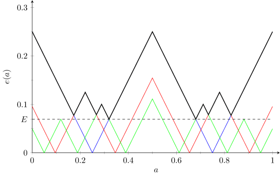
Figure 1: The functions $e(a)$ (black) and $e_{3}(a)$, $e_{5}(a),$ $e_{7}(a)$ (blue, red, green). The dashed line indicates the minimum value $E$ of the function $e(a)$.

Lemma 6

Fix any $a\in\left[0,1\right]$, $\varepsilon>0$, $n\in\left\{0,1,2,\ldots\right\}$, and take the angles $\theta_{a,\varepsilon,n}^{\flat},\theta_{a,\varepsilon,n}^{\sharp}\in\left[n\frac{\pi}{2},\left(n+1\right)\frac{\pi}{2}\right]$ such that

$$\sin^{2}(\theta_{a,\varepsilon,n}^{\flat})=\max\left(a-\varepsilon,0\right),\quad\sin^{2}(\theta_{a,\varepsilon,n}^{\sharp})=\min\left(a+\varepsilon,1\right).$$

Then

$$0<\varepsilon\leq e(a)$$ (40)

if an only if there is an $L\in\left\{3,5,7,\ldots\right\}$ such that

$$[L\theta_{a,\varepsilon,n}^{\flat},L\theta_{a,\varepsilon,n}^{\sharp}]\subset\left[m\frac{\pi}{2},\left(m+1\right)\frac{\pi}{2}\right]\quad\text{for some }m\in Ln+\left\{0,1,\ldots,L-1\right\}.$$ (41)

Proof. Condition (40) is satisfied if and only if there is an $L\in\left\{3,5,7,\ldots\right\}$ such that

$$0<\varepsilon\leq e_{L}(a).$$ (42)

Now observe that condition (42) holds whenever

$$a \in\left[0,\sin^{2}\left(\frac{1}{L}\frac{\pi}{2}\right)-\varepsilon\right]$$

$$\text{or\quad}a \in\left[\sin^{2}\left(\frac{1}{L}\frac{\pi}{2}\right)+\varepsilon,\sin^{2}\left(\frac{2}{L}\frac{\pi}{2}\right)-\varepsilon\right]$$

$$\vdots$$

$$\text{or\quad}a \in\left[\sin^{2}\left(\frac{L-2}{L}\frac{\pi}{2}\right)+\varepsilon,\sin^{2}\left(\frac{L-1}{L}\frac{\pi}{2}\right)-\varepsilon\right]$$

$$\text{or\quad}a \in\left[\sin^{2}\left(\frac{L-1}{L}\frac{\pi}{2}\right)+\varepsilon,1\right],$$

and so does condition (41). This proves the lemma.  

Remark 7

In fact, condition (40) is satisfied if and only if there is an $L\in\left\{3,5,7\right\}$ such that (41) holds. This is so because, for each $a\in\left[0,1\right]$, the maximum in (39) is attained at an $L\in\left\{3,5,7\right\}$ (which depends on $a$).

The largest possible value of $\varepsilon$ such that (40) holds for all $a\in\left[0,1\right]$ is denoted by $E$ . This value, indicated by the dashed horizontal line in Figure 1, is

$$E=\min_{a\in[0,1]}e(a)=\frac{1}{2}\left(\sin^{2}\left(\frac{3}{7}\frac{\pi}{2}\right)-\sin^{2}\left(\frac{1}{3}\frac{\pi}{2}\right)\right)\approx 0.06937,$$ (43)

with the minimum attained at $a=\frac{1}{2}\left(\sin^{2}\left(\frac{3}{7}\frac{\pi}{2}\right)+\sin^{2}\left(\frac{1}{3}\frac{\pi}{2}\right)\right)$. (Note that the minimum is also attained at $a=\frac{1}{2}\left(\sin^{2}\left(\frac{4}{7}\frac{\pi}{2}\right)+\sin^{2}\left(\frac{2}{3}\frac{\pi}{2}\right)\right)$.) By Lemma 6 and Remark 7, for every $a\in\left[0,1\right]$ and $\varepsilon\in(0,E]$, there is an $L\in\left\{3,5,7\right\}$ such that (41) holds.

We take

$$f(a,\varepsilon) =\frac{1}{2}|\theta_{a,\varepsilon,n}^{\sharp}-\theta_{a,\varepsilon,n}^{\flat}|$$

$$=\frac{1}{2}\left(\arcsin\sqrt{\min\left(a+\varepsilon,1\right)}-\arcsin\sqrt{\max\left(a-\varepsilon,0\right)}\right)$$

(where $\theta_{a,\varepsilon,n}^{\sharp},\theta_{a,\varepsilon,n}^{\flat}$ are defined in Lemma 6) as the accuracy of estimating the angle $\theta$ such that $\sin^{2}\theta=a$, expressed as a function of $a$ and the accuracy $\varepsilon>0$ of estimating $a\in\left[0,1\right]$. Note that $f(a,\varepsilon)$ does not depend on $n$. The graph of $f(a,E)$ is shown in Figure 2. We also put

$$F=\max_{a\in\left[0,1\right]}f(a,E),$$ (44)

indicated by the dashed horizontal line in Figure 2. The maximum is attained at $a=E$ (and also at $a=1-E$), so

$$F =f(E,E)=\frac{1}{2}\arcsin\sqrt{2E}$$

$$=\frac{1}{2}\arcsin\sqrt{\sin^{2}\left(\frac{3}{7}\frac{\pi}{2}\right)-\sin^{2}\left(\frac{1}{3}\frac{\pi}{2}\right)}\approx 0.19084,$$ (45)

This is the maximum accuracy of estimating $\theta$ when the accuracy of estimating $a=\sin^{2}\theta$ is$~{}E$.

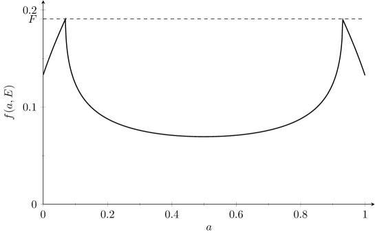
Figure 2: The function $f(a,E)$. The dashed line indicates the maximum value $F$.

4 Algorithm performance

The quantum computational complexity of the algorithm, which we denote by $M$, is understood as the number of applications of the operator $\mathbf{Q}$. We have shown that $M=O(\frac{1}{\varepsilon})$ for the QAE algorithms put forward in the present paper. In fact, the constants in our $O(\frac{1}{\varepsilon})$ bound for $M$ are low enough to outperform those in the earlier papers, in particular [Gri2021] and [Fuk2023]. This can be seen in Figure 3 by comparing the line labelled as $\mathrm{AQAE}_{M}$ computed from (6) in the present paper with the lines $\mathrm{IQAE}_{M}$ and $\mathrm{MIQAE}_{M}$ representing the bound

$$M<\frac{50}{\varepsilon}\ln\left(\frac{1}{\alpha}\log_{2}\left(\frac{\pi}{4\varepsilon}\right)\right)$$

for the IQAE algorithm of Grinko et al. [Gri2021], formula (8), and the bound

$$M<\frac{62}{\varepsilon}\ln\left(\frac{6}{\alpha}\right)$$

for the MIQAE algorithm of Fukuzawa et al. [Fuk2023], formula (3.32). Additionally, Figure 3 shows the bound $\mathrm{AQAE}_{\mathbb{E}(M)}$ on the expected value of $M$ obtained in Section 4.1 of the present paper.

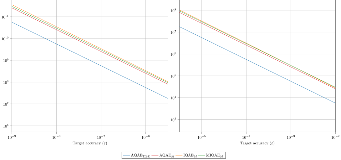
Figure 3: Bounds on quantum computational complexity $M$ depending on the target accuracy $\varepsilon$ as compared to the bounds for the IAQE algorithm [Gri2021] and the MIQAE algorithm [Fuk2023] in the case when $a=0.5$ and $\alpha=0.05$. A bound on the expectation $\mathbb{E}(M)$ for the AQAE algorithm is also shown (see Section 4.1).

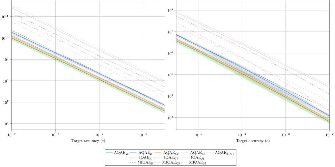
Figure 4: Quantum computational complexity $M$ depending on the target accuracy $\varepsilon$ as compared to the results from the IAQE algorithm [IQAE] and MIQAE algorithm [MIQAE] in the case when $a=0.5$ and $\alpha=0.05$. The values of $M$ are averages over 2000 runs of the algorithms. The shaded areas indicate the 25%–75% interquartile ranges. The gray lines show the theoretical bounds from Figure 3.

Numerical experiments to assess the performance of Algorithm 2 are presented in Figure 4 and compared with those from the Qiskit implementation [IQAE] of the IQAE algorithm and the implementation [MIQAE] of the MIQAE algorithm.

For an implementation of the AQAE algorithm, see [AQAE]. In addition to the Hoeffding confidence interval

$$[\max(\hat{A}_{i}^{N}-E_{i}^{N},0),\min(\hat{A}_{i}^{N}-E_{i}^{N},0)]$$

with $E_{i}$ given by (24) and $\hat{A}_{i}^{N}$ by (22), we also implement Algorithm 2 with the Clopper–Pearson confidence interval

$$\textstyle\left[B\left(\frac{\alpha_{i}}{2};n,N-n+1\right),B\left(1-\frac{\alpha_{i}}{2};n+1,N-n\right)\right],$$

where $B\left(p;a,b\right)$ is the $p$-th quantile of the beta distribution with shape parameters $a$ and $b$. In Figure 4 the lines for the AQAE, IQAE and MIQAE algorithms with Hoeffding and Clopper–Pearson confidence intervals are indicated by subscripts $H$ and $CP$, respectively. Because $M$, the number of applications of $\mathbf{Q}$, is random, we show the averages of $M$ over 2000 runs of the algorithms. To facilitate comparison, we show the 25%–75% interquartile ranges (rendered as shaded bands) for $M$ from our AQAE algorithm. This shows superior performance of Algorithm 2 compared to [IQAE] and [MIQAE], and therefore compared to all the earlier algorithms.

The Hoeffding and Clopper–Pearson confidence intervals are exact in the sense of guaranteeing the given confidence level for all possible values of the binomial distribution probability parameter being estimated. In doing so, they are also conservative. The performance of the algorithm can be improved further by allowing approximate confidence intervals, which are narrower and meet the prescribed confidence level approximately. This is possible because the sum $\sum_{i=0}^{I}\alpha_{i}$, for which $\alpha$ is an upper bound as shown in (28), in fact turns out significantly lower than $\alpha$ in numerical experiments. Here we implement Wilson’s score interval, the approximate confidence interval first proposed by Wilson [Wil1927] in 1927; see also [AgCo1998]:

$$\textstyle\left[\frac{\hat{A}_{i}^{N}+\frac{z_{\alpha_{i}/2}^{2}}{2N}-z_{\alpha_{i}/2}\sqrt{\frac{\hat{A}_{i}^{N}\left(1-\hat{A}_{i}^{N}\right)}{N}+\frac{z_{\alpha_{i}/2}^{2}}{4N^{2}}}}{1+\frac{z_{\alpha_{i}/2}^{2}}{N}},\frac{\hat{A}_{i}^{N}+\frac{z_{\alpha_{i}/2}^{2}}{2N}+z_{\alpha_{i}/2}\sqrt{\frac{\hat{A}_{i}^{N}\left(1-\hat{A}_{i}^{N}\right)}{N}+\frac{z_{\alpha_{i}/2}^{2}}{4N^{2}}}}{1+\frac{z_{\alpha_{i}/2}^{2}}{N}}\right],$$

where $z_{c}$ denotes the $1-c$ quantile of the standard normal distribution. Wilson’s score interval does indeed improve the performance of the algorithm still further, as can be seen in Figure 4, line $\mathrm{AQAE}_{W}$.

4.1 Computer-assisted bound for the expectation of $M$

The theoretical bound $\mathrm{AQAE}_{M}$ for the number of applications $M$ of $\mathbf{Q}$ is quite high compared to the results $\mathrm{AQAE}_{H}$ (and also $\mathrm{AQAE}_{CP}$ and $\mathrm{AQAE}_{W}$) of numerical experiments in Figure 4. Since $M$ is random in Algorithm 2, a bound for the expected value of $M$ would be more relevant. We achieve such a bound by first evaluating the expectation of the number of iterations $N_{i}^{\prime}$ of the inner loop for each round $i$ of the outer loop in Algorithm 2, conditioned on the algorithm outcomes for rounds $0,1,\ldots,i-1$ and on $I$. This involves computer-assisted computations of the binomial distribution probabilities of certain events.

The value of $N_{i}^{\prime}$ is obtained by running the inner loop in Algorithm 2. From $\alpha_{i}$ we compute $E_{i}^{N}$ using (24). According to Lemma 6, the inner loop stops at an iteration $N=N_{i}^{\prime}$ such that $E_{i}^{N}\leq e(\hat{A}_{i}^{N})$. This allows us to view $N_{i}^{\prime}$ as a random variable with values in $\{1,\ldots,N_{i}\}$ depending on $\alpha_{i}$, and to view the conditional expectation of $N_{i}^{\prime}$ as a function of $\alpha_{i}$.

We compute the probability $\mathbb{P}_{i}(E_{i}^{N}\leq e(\hat{A}_{i}^{N}))$ for each $N$ in $\{1,\ldots,N_{i}\}$, conditioned on the algorithm outcomes for rounds $0,1,\ldots,i-1$ and on $I$. Then we use these conditional probabilities to evaluate a bound for the expectation $\mathbb{E}_{i}(N_{i}^{\prime})$, also conditioned on the algorithm outcomes for rounds $0,1,\ldots,i-1$ and on $I$. Observe that $E_{i}^{N}\leq e(\hat{A}_{i}^{N})$ whenever $\hat{A}_{i}^{N}$ belongs to the union of the intervals depicted in Figure 5. This union of intervals will be denoted by $C_{i}^{N}$. We have $\hat{A}_{i}^{N}\in C_{i}^{N}$ iff $n\in NC_{i}^{N}$, where $n$ follows the binomial distribution $B(A_{i},N)$, that is, it is the number of successful outcomes in $N$ independent Bernoulli trials with probability of success $A_{i}$. This allows the conditional probability of $E_{i}^{N}\leq e(\hat{A}_{i}^{N})$ to be expressed as

$$\mathbb{P}_{i}(\hat{A}_{i}^{N}\in C_{i}^{N})=\mathbb{P}_{i}(E_{i}^{N}\leq e(\hat{A}_{i}^{N}))=\sum_{n\in NC_{i}}\binom{N}{n}A_{i}^{n}(1-A_{i})^{N-n}.$$

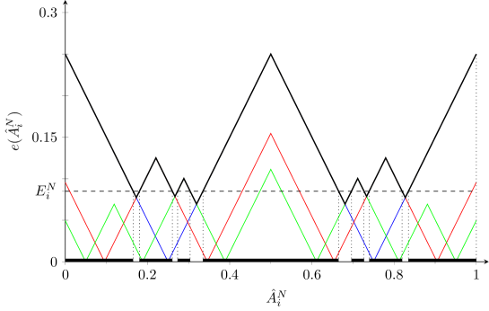
Figure 5: The set $C_{i}^{N}$ of values of $\hat{A}_{i}^{N}$ such that $E_{i}^{N}\leq e(\hat{A}_{i}^{N})$ is the union of the bold intervals on the horizontal axis.

Then, a bound for the conditional expectation $\mathbb{E}_{i}(N_{i}^{\prime})$ of the number of shots $N_{i}^{\prime}$ in the $i$th round of the outer loop can be obtained as follows. For any $J\in\left\{1,\ldots,N_{i}\right\}$, we have

$$\mathbb{E}_{i}(N_{i}^{\prime}) =\sum_{N=1}^{N_{i}}N\mathbb{P}_{i}\left(N=N_{i}^{\prime}\right)=\sum_{N=1}^{J}N\mathbb{P}_{i}\left(N=N_{i}^{\prime}\right)+\sum_{N=J+1}^{N_{i}}N\mathbb{P}_{i}\left(N=N_{i}^{\prime}\right)$$

$$\leq J\mathbb{P}_{i}\left(J\geq N_{i}^{\prime}\right)+N_{i}\mathbb{P}_{i}\left(J<N_{i}^{\prime}\right)\leq J+(N_{i}-J)\mathbb{P}_{i}\left(J<N_{i}^{\prime}\right).$$

Since $J<N_{i}$ implies that $E_{i}^{J}>e(\hat{A}_{i}^{J})$, it follows that

$$\mathbb{E}_{i}(N_{i}^{\prime})\leq J+(N_{i}-J)\mathbb{P}_{i}(E_{i}^{J}>e(\hat{A}_{i}^{J}))=J+(N_{i}-J)\left(1-\mathbb{P}_{i}(\hat{A}_{i}^{J}\in C_{i}^{J})\right).$$

This holds for each $J\in\left\{1,\ldots,N_{i}\right\}$, so

$$\mathbb{E}_{i}(N_{i}^{\prime})\leq\min_{J\in\left\{1,\ldots,N_{i}\right\}}\left(J+(N_{i}-J)\left(1-\mathbb{P}_{i}(\hat{A}_{i}^{J}\in C_{i}^{J})\right)\right).$$

This bound for $\mathbb{E}_{i}(N_{i}^{\prime})$ can be evaluated precisely. We use computer-assisted computations for this purpose, first to compute the probabilities $\mathbb{P}_{i}(\hat{A}_{i}^{J}\in C_{i}^{J})$ and then the minimum. For the Python code, see [CondExp]. The results are presented in Figure 6, which shows that

$$\mathbb{E}_{i}(N_{i}^{\prime})<\frac{1}{6}N_{i}+40.$$

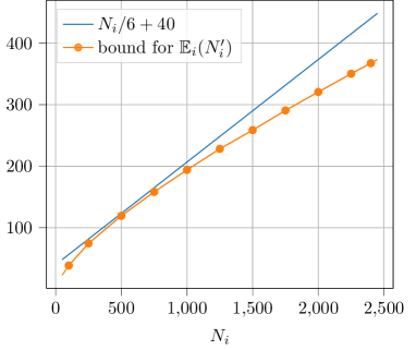
Figure 6: The expectation $\mathbb{E}_{i}(N_{i}^{\prime})$ computed for various values of $N_{i}$ versus the bound $\frac{1}{6}N_{i}+40$.

Now we can obtain a bound for the expectation $\mathbb{E}(M)$ of the number $M$ of applications of $\mathbf{Q}$, where

$$M=\sum_{i=0}^{I}\frac{K_{i}-1}{2}N_{i}^{\prime}<\frac{1}{2}\sum_{i=0}^{I}K_{i}N_{i}^{\prime}.$$

We have

$$\mathbb{E}(M|I) <\mathbb{E}\left(\left.\frac{1}{2}\sum_{i=0}^{I}K_{i}N_{i}^{\prime}\right|I\right)=\mathbb{E}\left(\left.\frac{1}{2}\sum_{i=0}^{I}K_{i}\mathbb{E}_{i}(N_{i}^{\prime})\right|I\right)$$

$$<\mathbb{E}\left(\left.\frac{1}{2}\sum_{i=0}^{I}K_{i}\left(\frac{1}{6}N_{i}+40\right)\right|I\right)=\mathbb{E}\left(\left.\frac{1}{12}\sum_{i=0}^{I}K_{i}N_{i}+20\sum_{i=0}^{I}K_{i}\right|I\right),$$

so

$$\mathbb{E}(M)<\mathbb{E}\left(\frac{1}{12}\sum_{i=0}^{I}K_{i}N_{i}+20\sum_{i=0}^{I}K_{i}\right).$$

By recycling some of the estimates at the end of the proof of Theorem 4, we obtain

$$\frac{1}{2}\sum_{i=0}^{I}K_{i}N_{i} <\frac{1}{\varepsilon}\left(\frac{1}{4E^{2}}\frac{\pi}{4}\left(\frac{3}{2}\ln\left(\frac{8}{C\alpha\pi}\right)+\frac{3}{4}\ln\left(3\right)\right)+\frac{3\pi}{16}\right),$$

$$\sum_{i=0}^{I}K_{i} <\sum_{i=0}^{I}3^{-I+i}\frac{\pi}{4}=\sum_{j=0}^{I}3^{-j}\frac{\pi}{4\varepsilon}<\frac{1}{\varepsilon}\frac{\pi}{6},$$

so

$$\mathbb{E}(M) <\frac{1}{\varepsilon}\left(\frac{1}{12}\left(\frac{1}{4E^{2}}\frac{\pi}{4}\left(\frac{3}{2}\ln\left(\frac{8}{C\alpha\pi}\right)+\frac{3}{4}\ln\left(3\right)\right)+\frac{3\pi}{16}\right)+\frac{20\pi}{6}\right)$$

$$\approx\frac{1}{\varepsilon}\left(27.380-10.201\ln\alpha\right).$$

This bound for $\mathbb{E}(M)$ is shown by the line labelled as $\mathrm{AQAE}_{\mathbb{E}(M)}$ in Figures 3 and 4. As expected, it is much tighter than the bound $\mathrm{AQAE}_{M}$ (hence even tighter than the bounds $\mathrm{IQAE}_{M}$ and $\mathrm{MIQAE}_{M}$) for $M$.

References

[Aar2020]S. Aaronson and P. Rall, Quantum approximate
counting, simplified, in Symposium on Simplicity in Algorithms, SIAM, 2020,
pp. 24–32. arXiv:1908.10846.
[AgCo1998]A. Agresti and B.A. Coull, Approximate is better
that “exact” for interval estimation,
The American Statistician52:2 (1998) 119–126.
[Bra2002]G. Brassard, P. Hoyer, M. Mosca, and A. Tapp,
Quantum Amplitude Amplification and Estimation, in: S.J. Lomonaco, Jr. and
H.E. Brandt (eds.), Quantum Computation and Information, AMS Special
Session (Washington, 19–21 January 2000), Contemporary Mathematics305 (2002) 53–74.
[Fuk2023]S. Fukuzawa, C. Ho, S. Irani, and J. Zion,
Modified iterative quantum amplitude estimation is asymptotically
optimal, arXiv:2208.14612v4 (2023).
[Gri2021]D. Grinko, J. Gacon, C. Zoufal, and S. Woerner,
Iterative quantum amplitude estimation, npj Quantum Inf.7
(2021) 52.
[Suz2020]Y. Suzuki, S. Uno, R. Raymond, T. Tanaka,
T. Onodera, and N. Yamamoto, Amplitude estimation without phase estimation,
Quantum Information Processing19:75 (2020) 1–17.
[Wil1927]E.B. Wilson, Probable inference, the law of
succession, and statistical inference, Journal of American Statistical
Association 22 (1927) 209–212.