Generalised Causal Dantzig

Abstract

Prediction invariance of causal models under heterogeneous settings has been exploited by a number of recent methods for causal discovery, typically focussing on recovering the causal parents of a target variable of interest. When instrumental variables are not available, the causal Dantzig estimator exploits invariance under the more restrictive case of shift interventions. However, also in this case, one requires observational data from a number of sufficiently different environments, which is rarely available. In this paper, we consider a structural equation model where the target variable is described by a generalised additive model conditional on its parents. Besides having finite moments, no modelling assumptions are made on the conditional distributions of the other variables in the system. Under this setting, we characterise the causal model uniquely by means of two key properties: the Pearson residuals are invariant under the causal model and conditional on the causal parents the causal parameters maximise the population likelihood. These two properties form the basis of a computational strategy for searching the causal model among all possible models. Crucially, for generalised linear models with a known dispersion parameter, such as Poisson and logistic regression, the causal model can be identified from a single data environment.

1 Introduction

Causal inference is the study of determining the causal relationship between two or more variables. This field has been a subject of research for many years, and its importance has only grown with the rise of artificial intelligence and machine learning (Pearl, 2019; Luo et al., 2020). Indeed, causal inference strategies go beyond prediction, ensuring that machine learning models have out-of-distribution generalization and a causal interpretation (Arjovsky et al., 2019). This is particularly important in applications such as healthcare and autonomous vehicles, where decisions made by machines have real-world consequences (Kuang et al., 2020).

In recent years, causal inference has been used extensively in social sciences (Sobel, 2000), economics (Varian, 2016), and public health (Glass et al., 2013) to determine the effectiveness of interventions and to inform policy decisions. For example, randomised controlled trials are commonly used in clinical studies to determine the causal effect of a treatment on a disease. However, conducting a randomised controlled trial is not always feasible or ethical. So, in some cases, observational studies must be used to infer causal relationships.

One popular method for causal inference in observational studies is propensity score matching (Haukoos and Lewis, 2015), which involves matching individuals who have similar characteristics and differ only in their exposure to a certain treatment or intervention. This technique has been used in various fields, such as education, finance, and healthcare, to determine the causal effect of a particular intervention. The focus of this propensity score matching is on the estimation of the causal effects, rather than the identification of the causal relationships. The latter is also referred to as causal discovery. An alternative approach to causal inference is the use of structural causal models (Pearl, 2009; Bollen and Pearl, 2013). These allow researchers also to model the causal relationships between variables, as well as to estimate the strength of these relationships. Within this framework, a number of methods have been developed for learning the causal graph from observational data, starting from the traditional PC-algorithm (Spirtes et al., 2001) and leading to various alternatives and extensions (Glymour et al., 2019). In many applications, learning the full causal graph is often too ambitious, while the interest is more focussed on discovering the direct causes of a certain variable of interest. This problem, which is also the focus of this paper, is sometimes referred to as causal feature selection (Guyon et al., 2007).

Embedded in the definition of structural causal models is the concept of causal invariance: the conditional distribution of a variable given its direct causes remains the same under perturbations on any other variable excluding the target variable itself. Causal invariance and the exclusion restriction assumptions are at the basis of invariant causal prediction. The method was recently proposed by Peters et al. (2016) to identify the causal relationships between variables in a system, and to predict the effect of an intervention on the system. The methodology is described primarily for the case of linear structural equation models and requires the availability of data across a number of sufficiently different environments. Searching for invariance across these environments results in conducting a number of statistical tests across all possible causal models. This can become computationally expensive for large systems. Various extensions have been proposed in recent years to address these limitations.

Rothenhäusler et al. (2019) avoids the combinatorial search by limiting the source of heterogeneity. They model perturbations as a system of linear structural equations, where covariates are shifted additively by an instrument. In that scenario, the covariance between the covariates and the residuals under the causal model remains invariant across datasets. Given access to two datasets with sufficiently different shifts, the difference between these invariant covariances provides a moment condition that uniquely identifies the causal model. Estimating the moment condition gives rise to the causal Dantzig estimator. One of the main drawbacks of the causal Dantzig is that the out-of-sample risk under the empirical estimator is often much larger than that of the ordinary least-squares estimator. This is due to the large variance of the causal Dantzig estimator, when the shifts in the different environments are small to moderate.

As a result of causal invariance, causal models enjoy the best out-of-sample prediction guarantees (Arjovsky et al., 2019). Some alternatives to invariant causal prediction focus more closely on this aspect. Rothenhäusler et al. (2021) find that the out-of-sample risk depends on the correlation between the residuals and the instrument. The more uncorrelated they are, the stronger the out-of-sample risk guarantees under unseen covariate shifts, whereby the causal model provides the best guarantees. Assuming access to the instrumental variable that generates the covariate shift, the authors propose to build a regularised estimator, called anchor regression, that regulates the amount of correlation between the residuals and the instrumental variable. While overcoming the issues of causal Dantzig, the main disadvantage of anchor regression is that it requires explicit information about the shift variables. This is often not available in observational studies.

Kania and Wit (2023) take a different view to anchor regression and aim for a solution that lies between the ordinary least-squares solution, which has the best in-sample risk guarantees, and the causal Dantzig solution, which has the best out-of-sample risk guarantees but which can be attained only with enough heterogeneity in the data. They avoid the need of instrumental variables by adding a regularization term to the likelihood that encourages causal invariance. A cross-validation strategy is proposed in order to find the best level of regularization from the available data.

Causal invariance approaches, and their theoretical guarantees, are mostly presented for the case of linear structural equation models, i.e., linear dependences between the variables and Gaussian distributed errors. A small number of studies have considered extensions to more general models. Bühlmann (2020) proposes an extension of anchor regression to the non-linear case, while Kook et al. (2022) consider the case of a transformation model (Hothorn et al., 2014) for the conditional distribution of the target variable given the parents. Similarly, invariant causal prediction has been extended to the non-linear case (Heinze-Deml et al., 2018) and to the case of time-ordered (Pfister et al., 2019) and general response types (Kook et al., 2023). In the latter case, a transformation model is again used for the conditional distribution of the target variable given the parents, while causal invariance is translated into an assumption of invariance of the expected conditional covariance between the environments and the score residuals. As with the linear equation models with Gaussian errors, these extensions are challenged by the requirement of observational data from a number of sufficiently different environments.

This paper proposes a new model-based approach for causal discovery for general response types which does not require multiple environments. In particular, we consider a structural equation model where the target variable is described by a generalised linear model conditional on its parents (McCullagh and Nelder, 1989). The link function can include flexible, possibly non-linear, additive modelling structures. As in Kook et al. (2023), no modelling assumptions are made on the other conditional distributions. Under this setting, we characterise the causal model uniquely by means of two key properties: invariance of the Pearson residuals and maximum of the population likelihood. As the expected squared Pearson residual of the causal model depends only on the dispersion parameter, causal generalised linear models with a known dispersion parameter, such as Poisson or logistic regression, can be identified from a single environment. Here, we will focus on these models. For other models, an estimate of the dispersion parameter can be used.

In section 2, we define the structural equation model formally and the characterization of the causal model describing the target variable. A computationally efficient strategy for detecting the causal model among all possible models from observational data is proposed. We call the resulting model the generalised causal Dantzig estimator of the causal model. Section 3 evaluates the performance of the method on simulation data in the case of Poisson additive regression and performs a comparison with the PC-algorithm. Section 4 shows the applicability of the proposed approach for the identification of the causal determinants of women’s fertility and high earning, using a Poisson and logistic additive regression setting, respectively.

2 Generalised causal Dantzig

In this section, we extend the causal Dantzig estimator. We begin by defining a structural equation model with exponential family target. Then we define a characterization of the causal model, that is unique under certain conditions. Given this characterization, we will define a population and empirical generalised causal Dantzig estimator of the causal model.

2.1 Structural equation model with exponential family target

We define a structural equation model that describes the dependences between a set of random variables. Let $Y$ be the target variable of interest and let $\boldsymbol{X}=(X_{1},\ldots,X_{p})^{\top}$ be the remaining variables in the system. The aim is to discover which of these variables are the causal parents of $Y$ and what their effect on $Y$ is. The following definition is considered for the joint distribution of $(\boldsymbol{X},Y)$.

Definition 1.

A structural equation model $(\boldsymbol{X},Y)$ with exponential dispersion family target $Y$ satisfies the following two conditions:

1. $(\boldsymbol{X},Y)$ is a causal graphical model (Lauritzen, 1996), i.e., it factorises w.r.t. a Directed Acyclic Graph (DAG) that represents the causal relationships between the variables and satisfies a do-calculus under intervention;

2. $Y|\boldsymbol{X}_{PA}=\boldsymbol{x}_{PA}\sim EDF\Big{(}b(f_{PA}(\boldsymbol{x}_{PA})),a(\phi)\Big{)}$ with $\boldsymbol{X}_{PA}$ the parents of $Y$ in the causal graph, where

   $$EDF(b(\theta),a(\phi))=\exp\bigg{\{}\frac{y\theta-b(\theta)}{a(\phi)}+c(y;\phi)\bigg{\}},\quad\quad\theta=f_{PA}(\boldsymbol{x}_{PA}),$$

   and $f_{PA}:\mathbb{R}^{|PA|}\rightarrow\mathbb{R}$ depends on $\boldsymbol{x}\in\mathbb{R}^{p}$ only through $\boldsymbol{x}_{PA}$, while $a(\cdot)$, $b(\cdot)$ and $c(\cdot)$ are known functions that define the distribution in the exponential dispersion family (McCullagh and Nelder, 1989).

Additional regularity conditions on $\boldsymbol{X}$ and $f_{PA}$, such as finite moments for $f_{PA}(\boldsymbol{X})$ in the case of Poisson distributed $Y$, as well as a strictly positive joint density $p(\boldsymbol{X})>0$, should be imposed depending on the the type of exponential family selected. We furthermore assume that the graph is faithful with respect to $Y$.

The distribution of $Y$ conditional on its parents is described by a generalised linear model with a canonical link, while no modelling assumptions are made on the distributions of the predictors $X_{i}$ given their parents. Notable examples in this family, frequently used on a variety of application studies, are Poisson and logistic regression. In both of these cases, $a(\phi)$ is known and equal to 1, while $b(\theta)=e^{\theta}$ for Poisson and $b(\theta)=\log(1+e^{\theta})$ for the logistic regression model. Note that in our definition of the model, linearity is not assumed in the distribution of $Y$ given $\boldsymbol{X}_{PA}$. The special case of $f_{PA}(\boldsymbol{x}_{PA})=\boldsymbol{\beta}_{PA}^{\top}\boldsymbol{x}_{PA}$ for some causal parameters $\boldsymbol{\beta}_{PA}$ may be of interest in practice, but the theoretical derivations do not assume this and apply also to more general models like generalised additive models (Wood, 2017).

2.2 Generalised causal Dantzig characterization of causal model

The structural equation model defined above contains a causal parameter, such as the infinite dimensional functional parameter $f_{PA}$ or the finite dimensional linear parameter $\boldsymbol{\beta}_{PA}$. The identification of this parameter identifies the causal structure governing $Y$. The next theorem describes the properties that characterise the causal model, that is the properties that are satisfied by $f_{PA}$.

Theorem 2.

Let $(\boldsymbol{X},Y)$ be distributed according to a structural equation model defined in definition 1. Let $\boldsymbol{X}_{PA}$ be the parents of $Y$ in this graph and $f_{PA}$ the true causal model linking $Y$ to its parents. Let $\dot{b}(\theta)$ and $\ddot{b}(\theta)$ be the first and second derivative of the cumulant generator function, respectively.

Then, $f_{PA}$ satisfies the following population conditions:

1. $f_{PA}$ is the maximiser of the expected population likelihood of $Y$ and its causal parents,

   $$f_{PA}=\arg\max_{f}\mathbb{E}_{\boldsymbol{X}_{PA},Y}\left[\ell_{\boldsymbol{X}_{PA},Y}(f)\right];$$

2. $f_{PA}$ achieves a perfectly dispersed population Pearson risk,

   $$\mathbb{E}_{\boldsymbol{X},Y}\left[\frac{(Y-\dot{b}(f_{PA}(\boldsymbol{X}_{PA})))^{2}}{\ddot{b}(f_{PA}(\boldsymbol{X}_{PA}))}\right]=a(\phi),$$

for any arbitrary square-integrable distribution of $\boldsymbol{X}$. In particular, this may be the observational or any interventional distribution.

Proof.

The first property is a direct consequence of the maximum likelihood estimator maximizing the expected log-likelihood, i.e., if we restrict the system to only $Y$ and its parents, then

$$\mathbb{E}_{\boldsymbol{X}_{PA},Y}\left[\ell_{\boldsymbol{X}_{PA},Y}(f)\right]=\mathbb{E}_{\boldsymbol{X}_{PA},Y}\bigg{[}\frac{Yf(\boldsymbol{X}_{PA})-b(f(\boldsymbol{X}_{PA}))}{a(\phi)}+c(Y;\phi)\bigg{]}$$

is maximised by $f_{PA}$.

As for the second property, using the laws of conditional probabilities, we can write the population Pearson risk as

$$\mathbb{E}_{\boldsymbol{X},Y}\bigg{[}\frac{(Y-\dot{b}(f_{PA}(\boldsymbol{X}_{PA})))^{2}}{\ddot{b}(f_{PA}(\boldsymbol{X}_{PA}))}\bigg{]}=\mathbb{E}_{\boldsymbol{X}_{PA}}\bigg{[}\mathbb{E}_{Y,\boldsymbol{X}_{{PA}^{C}}}\bigg{[}\frac{(Y-\dot{b}(f_{PA}(\boldsymbol{X}_{PA})))^{2}}{\ddot{b}(f_{PA}(\boldsymbol{X}_{PA}))}\bigg{|}\boldsymbol{X}_{PA}\bigg{]}\bigg{]}$$

where ${PA}^{C}$ is the complementary set of the parental set of $Y$, and hence $\boldsymbol{X}_{{PA}^{C}}$ are the non-causal variables. Recalling that the expected values in the population likelihood and Pearson risks are taken w.r.t. $(\boldsymbol{X},Y)$ distributed according to the true causal graphical model, we have in particular that $Y|\boldsymbol{X}_{PA}=\boldsymbol{x}_{PA}\sim EDF\Big{(}b(f_{PA}(\boldsymbol{x}_{PA})),a(\phi)\Big{)}$ for the chosen EDF distribution and $f_{PA}(\boldsymbol{X}_{PA})$ is only a function of $\boldsymbol{X}_{PA}$. Moreover, being a generalised linear model, it holds that $\mathbb{E}[Y|\boldsymbol{X}_{PA}]=\dot{b}(f_{PA}(\boldsymbol{X}_{PA}))$ and $\mathbb{V}ar[Y|\boldsymbol{X}_{PA}]=\ddot{b}(f_{PA}(\boldsymbol{X}_{PA}))a(\phi)$. Using these properties on the inner expectation, we can write the population Pearson risk as

$$\mathbb{E}_{\boldsymbol{X},Y}\bigg{[}\frac{(Y-\dot{b}(f_{PA}(\boldsymbol{X}_{PA})))^{2}}{\ddot{b}(f_{PA}(\boldsymbol{X}_{PA}))}\bigg{]}=\mathbb{E}_{\boldsymbol{X}_{PA}}\bigg{[}\frac{\ddot{b}(f_{PA}(\boldsymbol{X}_{PA}))a(\phi)}{\ddot{b}(f_{PA}(\boldsymbol{X}_{PA}))}\bigg{]}=a(\phi).$$

∎

The second property in Theorem 2 shows how the Pearson risk is invariant under the causal model, that is it is stable under any distribution of the covariates $\boldsymbol{X}$, including possible changes due to interventions. Unlike the quadratic risk used in the Gaussian case (Kania and Wit, 2023; Rothenhäusler et al., 2019), it is clear how an invariant property for generalised linear models must account also for their inherent heteroscedasticity. This is the role played by the conditional variance at the denominator of the Pearson risk. However, this invariance property can be satisfied by a number of other models. Considering for simplicity a generalised linear model with a linear predictor described by a $p+1$-dimensional vector of parameters $\boldsymbol{\beta}$, the set of solutions for which the Pearson risk condition is satisfied corresponds to a $p$ dimensional manifold in $\mathbb{R}^{p+1}$. The first condition in Theorem 2, stating that the causal model maximises the population likelihood of the marginal model $(\boldsymbol{X}_{PA},Y)$, guarantees an almost sure unique identification of the causal model within this surface, under the conditions described by the next theorem.

Theorem 3.

Let $S\subset\{1,\ldots,p\}$ indicate a potential set of causal parents of $Y$ in $\boldsymbol{X}$. Let $f_{S}:\mathbb{R}^{|S|}\rightarrow\mathbb{R}$ be the function that depends strictly on $\boldsymbol{X}_{S}$, and that satisfies (i) $f_{S}$ is defined on some functional space $\cal{F}$ with basis $\psi_{S}=\{\psi_{1},\psi_{2},\ldots\}$, i.e., $f_{S}(\boldsymbol{x}_{S})=\boldsymbol{\beta}_{S}^{\top}\psi_{S}(\boldsymbol{x}_{S})$, and (ii) $\boldsymbol{\beta}_{S}$ solves the population likelihood score equations

$$\mathbb{E}_{\boldsymbol{X}_{S},Y}\left[\psi_{S}(\boldsymbol{X}_{S})Y\right]-\mathbb{E}_{\boldsymbol{X}_{S},Y}\left[\psi_{S}(\boldsymbol{X}_{S})\dot{b}(\boldsymbol{\beta}^{\top}\psi_{S}(\boldsymbol{X}_{S}))\right]=0.$$

Then

$$S=PA\mbox{ and }f_{S}=f_{PA}\mbox{ a.s.}\quad\mbox{iff}\quad\mathbb{E}_{\boldsymbol{X},Y}\left[\frac{(Y-\dot{b}(\boldsymbol{\beta}_{S}^{\top}\psi_{S}(\boldsymbol{X}_{S})))^{2}}{\ddot{b}(\boldsymbol{\beta}_{S}^{\top}\psi_{S}(\boldsymbol{X}_{S}))}\right]=a(\phi).$$

Proof.

If $S=PA$ and $f_{S}=f_{PA}$ a.s., then Theorem 2 shows how $f_{PA}=\boldsymbol{\beta}_{PA}^{\top}\psi_{PA}$ satisfies the likelihood score equations from the first property and the Pearson risk invariance from the second property. We therefore only need to prove the reverse direction of this theorem.
Consider then a $\boldsymbol{\beta}_{S}$ that solves the score equations and that satisfies Pearson risk invariance. Then, since $\boldsymbol{\beta}_{S}^{\top}\psi_{S}$ depends only on $\boldsymbol{X}_{S}$, using similar derivations to before, we can rewrite the Pearson risk as

$$\mathbb{E}_{\boldsymbol{X},Y}\bigg{[}\frac{(Y-\dot{b}(\boldsymbol{\beta}_{S}^{\top}\psi_{S}(\boldsymbol{X}_{S})))^{2}}{\ddot{b}(\boldsymbol{\beta}_{S}^{\top}\psi_{S}(\boldsymbol{X}_{S}))}\bigg{]}=\mathbb{E}_{\boldsymbol{X}_{S}}\bigg{[}\frac{\mathbb{E}_{Y}[(Y-\dot{b}(\boldsymbol{\beta}_{S}^{\top}\psi_{S}(\boldsymbol{X}_{S})))^{2}|\boldsymbol{X}_{S}]}{\ddot{b}(\boldsymbol{\beta}_{S}^{\top}\psi_{S}(\boldsymbol{X}_{S}))}\bigg{]}.$$

Thus, except for a null set on the space of distributions on $\boldsymbol{X}_{S}$, Pearson risk invariance can be achieved only if

$$\mathbb{E}_{Y}[(Y-\dot{b}(\boldsymbol{\beta}_{S}^{\top}\psi_{S}(\boldsymbol{X}_{S})))^{2}|\boldsymbol{X}_{S}]=\ddot{b}(\boldsymbol{\beta}_{S}^{\top}\psi_{S}(\boldsymbol{X}_{S}))a(\phi).$$

Multiplying both sides of the equation by $\psi_{S}(\boldsymbol{X}_{S})$ and dividing by $a(\phi)^{2}$, we have

$$\frac{\mathbb{E}_{Y}[\psi_{S}(\boldsymbol{X}_{S})^{\top}(Y-\dot{b}(\boldsymbol{\beta}_{S}^{\top}\psi_{S}(\boldsymbol{X}_{S})))^{2}\psi_{S}(\boldsymbol{X}_{S})|\boldsymbol{X}_{S}]}{a(\phi)^{2}}=\frac{\psi_{S}(\boldsymbol{X}_{S})^{\top}\ddot{b}(\boldsymbol{\beta}_{S}^{\top}\psi_{S}(\boldsymbol{X}_{S}))\psi_{S}(\boldsymbol{X}_{S})}{a(\phi)}.$$

Since $Y-\dot{b}(\boldsymbol{\beta}_{S}^{\top}\psi_{S}(\boldsymbol{X}_{S}))$ is a scalar, we can further rewrite the left hand side as an inner product, resulting in

$$\mathbb{E}_{Y}\bigg{[}\frac{(\psi_{S}(\boldsymbol{X}_{S})(Y-\dot{b}(\boldsymbol{\beta}_{S}^{\top}\psi_{S}(\boldsymbol{X}_{S})))^{\top}}{a(\phi)}\frac{\psi_{S}(\boldsymbol{X}_{S})(Y-\dot{b}(\boldsymbol{\beta}_{S}^{\top}\psi_{S}(\boldsymbol{X}_{S})))}{a(\phi)}|\boldsymbol{X}_{S}\bigg{]}$$

$$=\frac{\psi_{S}(\boldsymbol{X}_{S})^{\top}\ddot{b}(\boldsymbol{\beta}_{S}^{\top}\psi_{S}(\boldsymbol{X}_{S}))\psi_{S}(\boldsymbol{X}_{S})}{a(\phi)}.$$

Taking now expectation w.r.t. $\boldsymbol{X}_{S}$ we have that

$$\mathbb{E}_{\boldsymbol{X}_{S}}\bigg{[}\mathbb{E}_{Y}\bigg{[}\frac{(\psi_{S}(\boldsymbol{X})(Y-\dot{b}(\boldsymbol{\beta}_{S}^{\top}\psi_{S}(\boldsymbol{X}_{S}))))^{\top}}{a(\phi)}\frac{\psi_{S}(\boldsymbol{X}_{S})(Y-\dot{b}(\boldsymbol{\beta}_{S}^{\top}\psi_{S}(\boldsymbol{X}_{S})))}{a(\phi)}|\boldsymbol{X}_{S}\bigg{]}\bigg{]}$$

$$=\mathbb{E}_{\boldsymbol{X}_{S}}\bigg{[}\psi_{S}(\boldsymbol{X}_{S})^{\top}\frac{\ddot{b}(\boldsymbol{\beta}_{S}^{\top}\psi_{S}(\boldsymbol{X}_{S}))}{a(\phi)}\psi_{S}(\boldsymbol{X}_{S})\bigg{]}.$$

We finally notice how the LHS is the expected value of the expected square of the gradient of the maximum log-likelihood of an EDF distribution, since $\boldsymbol{\beta}_{S}$ solves the score equations by assumption. The right hand side is the expected value of the expected Fisher information matrix on $\boldsymbol{\beta}_{S}$ of the same EDF distribution. The two sides match if and only if

$$Y\>|\>\boldsymbol{X}_{S}\sim EDF(b(\boldsymbol{\beta}_{S}^{\top}\psi_{S}(\boldsymbol{X}_{S})),a(\phi)).$$

Except for a null set on the space of distributions on $\boldsymbol{X}_{S}$, under the true graphical model this is true only if $S=PA$ and $f_{S}=f_{PA}$. ∎

Remark 4.

Uniqueness is achieved under the restriction that $f_{S}$ depends on all $\boldsymbol{x}_{S}$ — in Theorem 3 this was referred to as strict dependence on $\boldsymbol{x}$. Any set $\boldsymbol{X}_{S}$ that contains $\boldsymbol{X}_{PA}$ together with variables that are d-separated from $Y$ by its parents would still satisfy the two properties that characterise the causal model. This is because $f_{S}$ is simply constant with respect to these variables.

In the next section, we propose a computational strategy for the search of the causal model based on the characterization that we have provided above and addressing the redundancy in the candidate models that we have just remarked.

1. For any set of covariates $\boldsymbol{X}_{S}$, with $S\subset\{1,\ldots,p\}$, determine the population maximum likelihood,

   $$\boldsymbol{\beta}_{S}=\arg\max_{\boldsymbol{\beta}}\mathbb{E}_{\boldsymbol{X}_{S},Y}[\ell_{\boldsymbol{X}_{S},Y}(\boldsymbol{\beta})].$$

2. Check whether the Pearson risk is perfectly dispersed for $\boldsymbol{\beta}_{S}$, that is whether

   $$\mathbb{E}_{\boldsymbol{X},Y}\left[\frac{(Y-\dot{b}(\boldsymbol{\beta}_{S}^{\top}\psi_{S}(\boldsymbol{X}_{S})))^{2}}{\ddot{b}(\boldsymbol{\beta}_{S}^{\top}\psi_{S}(\boldsymbol{X}_{S}))}\right]=a(\phi).$$

   If it is, then $\boldsymbol{\beta}_{S}^{\top}\psi_{S}$ is a candidate for $f_{PA}=\boldsymbol{\beta}_{PA}^{\top}\psi_{PA}$.

3. Among the set of candidate models $\boldsymbol{\beta}_{S}$, select $\boldsymbol{\beta}_{PA}$ as the one minimising the Bayesian Information Criterion (BIC).

Algorithm 1 Population algorithm for finding causal parents.

2.3 Population and empirical algorithms

Theorem 3 can be translated into a population algorithm for finding the causal model. It involves a combinatorial search among all subsets of covariates, and is described in Algorithm 1. The algorithm involves a search of the models that achieve a perfectly dispersed Pearson risk. Then, an information criterion is used to select the optimal model among the class of candidate models. The choice of an information criterion is motivated by the fact that variables that are d-separated from $Y$ by its causal parents, such as ancestors of $Y$, have no predictive power on $Y$. In principle, any information criterion that penalises the expected likelihood by a term including the number of covariates can be used at this stage.

For a finite sample, $(\boldsymbol{x}_{i},y_{i})$, $i=1,\ldots,n$, an empirical version of the population algorithm is proposed in Algorithm 2. It involves replacing the population likelihood by the empirical likelihood, while the requirement of a perfectly dispersed Pearson risk is checked via an appropriate statistical test. In particular, for each candidate subset $\boldsymbol{X}_{S}$, we test the null hypothesis

$$H_{0}:\mathbb{E}_{\boldsymbol{X},Y}\left[\frac{(Y-\dot{b}({\boldsymbol{\beta}_{S}}^{\top}\psi_{S}(\boldsymbol{X}_{S})))^{2}}{\ddot{b}({\boldsymbol{\beta}_{S}}^{\top}\psi_{S}(\boldsymbol{X}_{S}))}\right]=a(\phi).$$

We consider a $q$-dimensional basis $\tilde{\psi}_{S}$ for $\{f:\mathbb{R}^{|S|}\rightarrow\mathbb{R}~{}|~{}f=\beta^{\top}\tilde{\psi}_{S}\}$. Typical examples are (i) a simple linear basis, in which case $q=|S|$, or (ii) a simple additive model with individual $q_{0}$-dimensional bases for each of the variables, in which case $q=q_{0}|S|$. For this, we use the test statistic

$$R^{+}=\displaystyle\sum_{i=1}^{n}\left[\frac{(y_{i}-\dot{b}({\widehat{\boldsymbol{\beta}}}_{S}^{\top}\tilde{\psi}_{S}(\boldsymbol{x}_{i,S})))^{2}}{\ddot{b}({{\widehat{\boldsymbol{\beta}}}_{S}}^{\top}\tilde{\psi}_{S}(\boldsymbol{x}_{i,S}))a(\phi)}\right],$$

where $\boldsymbol{x}_{i,S}$ denotes the $i$-th realization of $\boldsymbol{X}_{S}$ and $\widehat{\boldsymbol{\beta}}_{S}$ is a penalised maximum likelihood estimator,

$$\widehat{\boldsymbol{\beta}}_{S}=\arg\max_{\boldsymbol{\beta}}\sum_{i=1}^{n}\frac{y_{i}\boldsymbol{\beta}^{\top}\tilde{\psi}_{S}(\boldsymbol{x}_{i,S})-b(\boldsymbol{\beta}^{\top}\tilde{\psi}_{S}(\boldsymbol{x}_{i,S}))}{a(\phi)}+\lambda P_{\lambda}(\boldsymbol{\beta}),$$

for some convenient smoothness or sparsity penalty $P_{\lambda}$ (Wood, 2017). Under the null hypothesis and some standard conditions on the penalty, the Pearson statistic is asymptotically chi-squared distributed. In particular, it holds that, approximately,

$$R^{+}\overset{H_{0}}{\sim}\chi^{2}_{n-\hat{q}},$$ (1)

with $\hat{q}$ an estimate for the effective degrees of freedom of the model.

1. For any set of covariates $\boldsymbol{X}_{S}$, with $S\subset\{1,\ldots,p\}$, find the penalised maximum likelihood estimator,

   $$\widehat{\boldsymbol{\beta}}_{S}=\arg\max_{\boldsymbol{\beta}}\sum_{i=1}^{n}\frac{y_{i}\boldsymbol{\beta}^{\top}\tilde{\psi}_{S}({\boldsymbol{x}_{i}}_{S})-b(\boldsymbol{\beta}^{\top}\tilde{\psi}_{S}({\boldsymbol{x}_{i}}_{S}))}{a(\phi)}+\lambda P_{\lambda}(\boldsymbol{\beta}),$$

   for a finite dimensional basis $\tilde{\psi}_{S}$.

2. Find $S_{1},\ldots,S_{K}\subset\{1,\ldots,p\}$ such that

   $$H_{0}:\mathbb{E}_{\boldsymbol{X},Y}\left[\frac{(Y-\dot{b}({\boldsymbol{\beta}_{S}}_{k}^{\top}\psi_{S}(\boldsymbol{X}_{S})))^{2}}{\ddot{b}({\boldsymbol{\beta}_{S}}_{k}^{\top}\psi_{S}(\boldsymbol{X}_{S}))}\right]=a(\phi)$$

   cannot be rejected, i.e., such that

   $$\chi^{2}_{n-\hat{q}_{k},\frac{\alpha}{2}}\leq\displaystyle\sum_{i=1}^{n}\left[\frac{(y_{i}-\dot{b}({\widehat{\boldsymbol{\beta}}}_{S_{k}}^{\top}\tilde{\psi}_{S_{k}}(\boldsymbol{x}_{i,S_{k}})))^{2}}{\ddot{b}({{\widehat{\boldsymbol{\beta}}}_{S_{k}}}^{\top}\tilde{\psi}_{S_{k}}(\boldsymbol{x}_{i,S_{k}}))a(\phi)}\right]\leq\chi^{2}_{n-\hat{q}_{k},1-\frac{\alpha}{2}},$$

   for some significance level $\alpha$, where $\hat{q}_{k}$ is the effective degrees of freedom of the model involving $S_{k}$.

3. Among the set of candidate models $f_{S_{1}},\ldots,f_{S_{K}}$, select $f_{PA}$ as the one minimising the Bayesian Information Criterion (BIC).

Algorithm 2 Empirical algorithm for finding causal parents.

The algorithm considers all possible models and retains those for which the null hypothesis cannot be rejected. As the aim is to select perfectly dispersed models, a two-sided test is needed and therefore the acceptance region for the model that includes variables $S_{k}$ is given by

$$\chi^{2}_{n-\hat{q}_{k},\frac{\alpha}{2}}\leq\displaystyle\sum_{i=1}^{n}\left[\frac{(y_{i}-\dot{b}({\widehat{\boldsymbol{\beta}}}_{S_{k}}^{\top}\tilde{\psi}_{S_{k}}(\boldsymbol{x}_{i,S_{k}})))^{2}}{\ddot{b}({{\widehat{\boldsymbol{\beta}}}_{S_{k}}}^{\top}\tilde{\psi}_{S_{k}}(\boldsymbol{x}_{i,S_{k}}))a(\phi)}\right]\leq\chi^{2}_{n-\hat{q}_{k},1-\frac{\alpha}{2}},$$

for some significance level $\alpha$, where $\hat{q}_{k}$ is the effective degrees of freedom associated with the model involving $S_{k}$. As with the population algorithm, the candidate set of models obtained via statistical testing is finally refined via BIC, in order to find the sparse most predictive model among the class of perfectly dispersed models.

Looking at all possible models leads to a computational complexity of the algorithm that is exponential. For real applications involving a large number of covariates, we therefore propose also a stepwise version of the algorithm. At each step, we add the variable with the largest p-value from the statistical test (1) and stop when the addition of the new variable decreases the p-value of the resulting model and drops below the significance level $\alpha$.

3 Simulation study

In this section, we illustrate the performance of the generalised causal Dantzig procedure. In section 3.1, we describe the data generating process for a generalised additive target inside a structural equation model. In section 3.2 we explain the idea behind Theorem 2 as the characterization of the causal parameters in the population scenario by means of a large sample. Finally in section 3.3 we show the performance of the method in a non-linear Poisson regression setting for the target of interest.

3.1 Simulating data via an underlying SEM

We generate a sample $(\boldsymbol{x}_{i},y_{i})$, $i=1,\ldots,n$ from a structural equation model with exponential target in definition 1 by first simulating $(\boldsymbol{x}_{i},z_{i})$ observations from a linear structural equation model (SEM), as follows,

$$\begin{bmatrix}Z\\ \boldsymbol{X}\\ \end{bmatrix}=B\begin{bmatrix}Z\\ \boldsymbol{X}\\ \end{bmatrix}+\begin{bmatrix}\epsilon_{Z}\\ \boldsymbol{\epsilon}_{X}\\ \end{bmatrix}$$ (2)

where $B=\begin{bmatrix}0&\boldsymbol{b}_{PA}^{\top}\\ \boldsymbol{\beta}_{CH}&B_{X}\\ \end{bmatrix}$ is the matrix of unknown parameters describing the structural equations between the variables $(\boldsymbol{X},Z)$, such that $(I-B)$ is invertible, and $\epsilon_{Z}\sim N(0,\sigma^{2}_{Z})$ and $\epsilon_{j,X}\sim N(0,\sigma_{j}^{2}))$ are independent noise components ($j=1,\ldots,p$). The exponential family target variables $Y_{i}$ are then simulated via

$$y_{i}=F^{-1}_{b(\boldsymbol{\beta}_{PA}^{\top}\boldsymbol{x}_{i,PA}),a(\phi)}(\Phi_{0,\sigma^{2}_{Z}}(\epsilon_{i,Z})),$$ (3)

where $F_{b(\boldsymbol{\beta}_{PA}^{\top}\boldsymbol{x}_{i,PA}),a(\phi)}$ is the cdf of the EDF distribution and $\Phi_{m,s^{2}}$ is the cdf of a $N(m,s^{2})$ distribution. In this notation, $\boldsymbol{\beta}_{PA}$ is the vector of non-zero coefficients corresponding to a causal generalised linear model for the target variable $Y$. The vector $\boldsymbol{b}_{PA}\in\mathbb{R}^{p}$ is identical to $\boldsymbol{\beta}_{PA}$, but also includes additional zeroes for the variables that are not the causal parents.

This formulation of the model allows to control the predictive power of the children of $Y$ via the underlying linear SEM (2), where the variable $Z$ is in the same scale as the predictors $\boldsymbol{X}$. In this way, we can make the detection of the causal parameters $\boldsymbol{\beta}_{PA}$ sufficiently different from the standard regression approaches. Figures 1a and 1c show two causal DAGs that will be used in the simulations in the next two sections. The left plots show the causal graphs of $(\boldsymbol{X},Y)$, while the right plots show the DAGs corresponding to the equivalent formulation as a linear SEM on $(\boldsymbol{X},Z)$. The transformation (3) guarantees that $Y$ has the required distribution, i.e.,

$$Y|\boldsymbol{X}_{PA}=\boldsymbol{x}_{PA}\sim EDF\Big{(}b(\boldsymbol{\beta}_{PA}^{\top}\boldsymbol{x}_{PA}),a(\phi)\Big{)},$$

with the parents of $Y$ being the parents of $Z$ in the SEM. In the simulation studies, we will consider Poisson regression as a running example.

(a)

(b)

(c)

(d)

Figure 1: Left: Causal graphical models for generating data on a target variable $Y$ and (a) p=2 (c) p=7 predictors. (b), (d): Equivalent formulations of (a),(c), respectively, with a latent variable $Z$, a linear SEM on $(\boldsymbol{X},Z)$ and a transformation of $Z$ in a $Y$ with a given EDF distribution conditional on $\boldsymbol{X}_{PA}$.

3.2 Proof-of-concept: population scenario

In this section, we highlight the main features of the proposed method via a simple simulation. We consider the DAG in Figure 1(a), with a target variable $Y$ having a causal parent $X_{1}$ and a child $X_{2}$. We consider a Poisson distribution for $Y$ conditional on $X_{1}$ and an underlying structural equation model (Figure 1(b)) given by

$$\begin{cases}X_{1}&=\epsilon_{1}\\ Z&=X_{1}+\epsilon_{Z}\\ X_{2}&=Z+\epsilon_{2},\end{cases}$$

where we assume the noise components $\epsilon_{1}$, $\epsilon_{2}$ and $\epsilon_{Z}$ to be independent and identically distributed standard normal random variables. From the structural equations, we deduce that $\boldsymbol{b}_{PA}=(1,0)^{\top}$, with the causal parameter $\beta_{PA}=1$, so

$$Y|X_{PA}=x_{PA}\sim\mbox{Poisson}(e^{X_{1}}).$$

We simulate a dataset from this system with a large sample size ($n=100000$), i.e., mimicking the population setting. Figure 2(a) shows the contour lines of the likelihood function of a full model, with both $X_{1}$ and $X_{2}$ being potential parents to $Y$. Since $Y$ has a conditional Poisson distribution and considering only the terms dependent on $\boldsymbol{\beta}$, this is given by

$$\ell(\boldsymbol{\beta})=\frac{1}{n}\sum_{i=1}^{n}[y_{i}\boldsymbol{\beta}^{\top}\boldsymbol{x}_{i}-e^{\boldsymbol{\beta}^{\top}\boldsymbol{x}_{i}}].$$

For easy of visualization, we consider a full model without the intercept, and so a $\boldsymbol{\beta}$ vector of length 2. As expected, Figure 2(a) shows how the Maximum Likelihood (ML) estimate of $\boldsymbol{\beta}$ achieves the maximum of this function, being the most predictive model on the observed data. On the other hand, the causal parameter $\boldsymbol{b}_{PA}$ lies on a lower contour line.

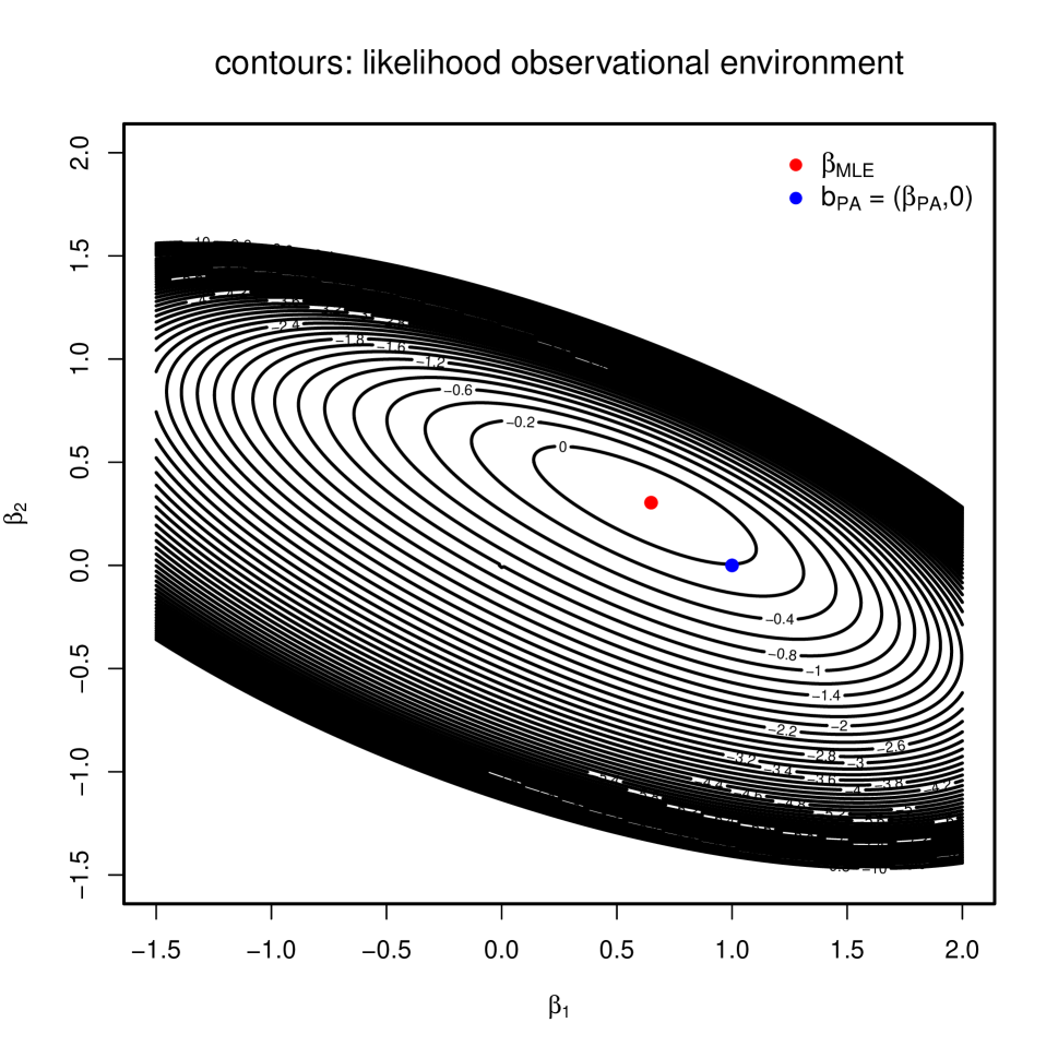
(a)

(b)

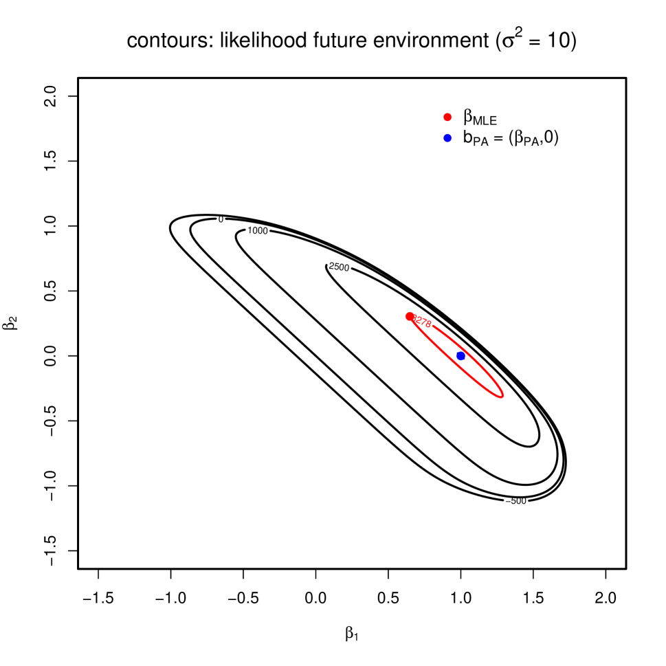
(c)

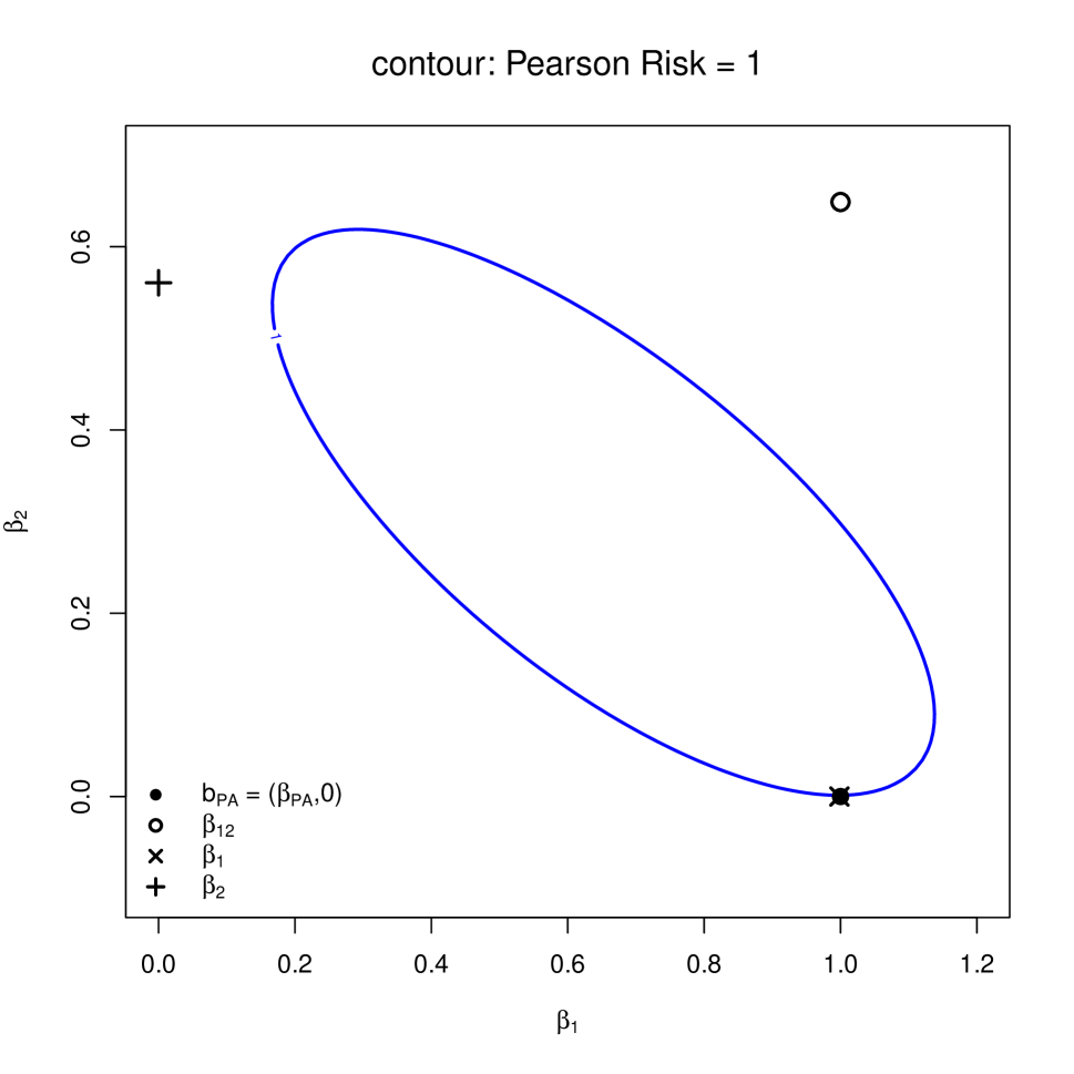
(d)

Figure 2: Simulated data ($n=100000$) using a Poisson regression model with $p=2$ predictors. Contour lines of likelihood on (a) observational data and (b)-(c) two future environments, with covariates $X_{1}$ and $X_{2}$ perturbed by an additive noise with variance $\sigma^{2}=5$ and $\sigma^{2}=10$, respectively. The MLE solution (red dot) has a higher likelihood than the causal solution (blue dot) on the observational environment (a) but a lower likelihood on the shifted environments (b-c), particularly for larger noise (c). That is, the causal model has better out-of-sample guarantees. (d) Contour line for Pearson risk $=1$ contains the true $\boldsymbol{b}_{PA}$, which coincide with the ML $\boldsymbol{\beta}_{1}$ of the model that includes only the causal parent $X_{1}$. The ML population estimates $\boldsymbol{\beta}_{S}$ from other models are not on the Pearson risk $=1$ surface.

The situation changes if one evaluates the prediction performance of the models on out-of-sample data. In particular, we consider the case where $X_{1}$ and $X_{2}$ are perturbed by an additional $N(0,\sigma^{2})$ noise. Figures 2(b) and 2(c) show the cases of $\sigma^{2}$ equal to $5$ and $10$, respectively. It is evident how the likelihood of the $\boldsymbol{\beta}_{MLE}$ model evaluated on the out-of-sample data is now lower compared to that evaluated on the causal solution. This is more pronounced in Figure 2(c) than in Figure 2(b), that is the larger the perturbation is. This shows, firstly, how causal models have better out-of-sample guarantees than predictive models, and, secondly, how maximising the likelihood on observational data is not an appropriate criterion for causal discovery. Both facts are well-known in the causal inference literature (e.g., Kania and Wit, 2023).

Figure 2(d) shows the surface satisfied by all $\boldsymbol{\beta}$ with Pearson risk equal to 1. As expected from Theorem 2, $\boldsymbol{b}_{PA}$ belongs to this surface, and so does the $\boldsymbol{\beta}_{1}$, the population maximum likelihood estimator of the dependence of $Y$ only on the causal parent $X_{1}$. The remaining two models, i.e., the saturated model ($\beta_{12}$) and the model with $Y$ dependent only on $X_{2}$ ($\beta_{2}$), lead to population maximum likelihood estimates that do not lie on the Pearson risk surface. Indeed, these models are not causal and, therefore, do not enjoy the invariance property, as shown in the uniqueness result of Theorem 3.

3.3 Finite sample behaviour of generalised causal Dantzig

In this section, we study the behaviour of the finite sample algorithm to obtain the causal parents of target $Y$. We consider the more complex system in Figure 1(c), where $Y$ has 2 causal parents ($X_{2}$ and $X_{3}$) and with 5 other variables in the system. We simulate it according to a latent structural equation model shown in Figure 1(d), where

$$\begin{cases}X_{1}&=\epsilon_{1}\\ X_{2}&=X_{1}+\epsilon_{2}\\ X_{3}&=X_{1}+X_{2}+\epsilon_{3}\\ Z&=\sin(5X_{2})+X_{3}^{3}+\epsilon_{Z}\\ X_{4}&=X_{2}+\epsilon_{4}\\ X_{5}&=Z+\epsilon_{5}\\ X_{6}&=Z+\epsilon_{6}\\ X_{7}&=X_{6}+\epsilon_{7}\\ \end{cases}.$$

In particular, the non-linear predictor for the target $Y$ is described by the function $f_{PA}(x_{2},x_{3})=\sin(5x_{2})+x_{3}^{3}$. The error terms are assumed to be independent and normally distributed with mean 0 and variance 0.04. For the distribution of $Y$ given $X_{2}$ and $X_{3}$, we consider a Poisson regression model, i.e.,

$$Y|\boldsymbol{X}_{PA}=\boldsymbol{x}_{PA}\sim\mbox{Poisson}\Big{(}e^{f_{PA}(\boldsymbol{x}_{PA})}\Big{)}.$$

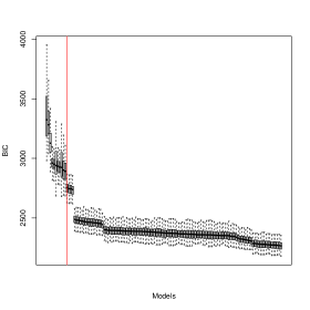
(a)

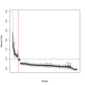
(b)

(c)

		PC-algorithm
$n$	GCD	$X_{2}\rightarrow Y\leftarrow X_{3}$	$X_{2}\rightarrow Y$	$Y\leftarrow X_{3}$
1000	91%	9%	24%	16%
500	80%	0%	14%	1%
250	60%	0%	11%	2%
200	49%	0%	9%	0%
150	27%	0%	2%	0%
100	8%	0%	1%	0%

(d)

Figure 3: Results across 100 simulations with $n=1000$ from the Model in Figure 1(c) with a Poisson distribution for $Y$ conditional on its causal parents. (a) BIC values across all models show how the causal model (red vertical line) is not the one that minimises BIC; (b) Pearson risk values show how the causal model has a median Pearson risk close to 1; (c) % times a model is selected by a Generalised Causal Dantzig approach using a 5% significance level shows a high percentage for the causal model; (d)The table reports the percentage of times that the correct model is selected by the proposed Generalised Causal Dantzig (GCD) approach. For the PC-algorithm, we count the graphs where there is a direct arrow to the target $Y$ from its parents ($X_{2}$, $X_{3}$), as well as those where only one of the two arrows is detected. Across all settings, the proposed method detects the true causal model more often than the PC-algorithm.

We repeat the simulation 100 times with sample size $n=1000$. We fit Poisson regression models for $Y$ for all possible subsets of the predictors. In order not to use any information from the generative process, we include also an intercept term in each of these models. Figure 3(a) shows the boxplots of BIC values of the models across the 100 simulations, sorted in descending order according to their median. The figure shows how the causal model (red vertical line) is far from being the most predictive model on the observational data. Indeed, the model with the lowest median BIC value is a model that includes the parents of $Y$ ($X_{2}$ and $X_{3}$) as well as its children ($X_{5}$ and $X_{6}$), which form the Markov blanket of $Y$ in the graph in Figure 1(c). On the other hand, Figure 3(b) shows how the causal model achieves a median Pearson risk close to 1, together with 3 other models that contain either ancestors ($X_{1}$) or variables blocked by the parents of $Y$ ($X_{4}$). Figure 3(c) shows how the generalised causal Dantzig procedure is able to detect the correct causal model 91% of the time out of all models, when setting an $\alpha=5\%$ in the statistical testing procedure.

Figure 3(d) shows how the detecting accuracy changes for decreasing sample sizes $n$. As expected, the accuracy in detecting the causal model decreases with $n$. However, it is significantly larger than what can be achieved with the PC-algorithm. As there are no implementations of the PC-algorithm that are specific to systems with Gaussian variables and a target count variable, we stabilised the variance of $Y$ by taking a square-root transformation and constructed the causal graph using Gaussian conditional independence tests on the resulting data.

4 Identifying causal drivers in two empirical studies

Here we illustrate the use of the generalised causal Dantzig method on two empirical studies. In section 4.1 we consider data from a women’s fertility study in the US. The aim is to identify the causal drivers of women’s reproductive fertility. In section 4.2 we consider a socio-economic study for identifying potential causal drivers of high income.

4.1 Causal determinants of fertility

The National Opinion Resource Center’s General Social Survey, which is currently available for 34 editions between 1972 and 2022 (GSS, 2022), can be used for the identification of the causal determinants of women’s fertility. The survey is conducted on English-speaking women living in non-institutional arrangements in the United States. As in Sander (1992), we consider women between the age of $35$ and $54$, as younger women may not have completed their schooling or their reproductive period. Across the $34$ editions of the survey, this results in a sample size of $n=16,269$ women. The target variable of interest is the “number of children ever born,” whereas the potential causal determinants are investigated among $p=8$ available covariates:

• level of education: years of schooling, mother’s years of schooling, father’s years of schooling (ordinal variables taking integer values between 0 and 20);

• demographic variables: age, race (indicator variable for black), region of the country at age 16 (south, east, north-center, west), living environment at age 16 (farm, other rural, town, small city, large city);

• time: the year of the study.

We fit an additive Poisson regression model with all variables, where we consider thin-plate regression splines for the 5 numerical variables (years of schooling, mother’s and father’s years of schooling, year of study, age) and factorial main effects for the remaining 3 categorical variables. The variables produce a relatively good fit, with 8.04% of deviance explained. The results correspond to other association studies conducted in the literature, with years of schooling, age, race, living environment and years of study picked up as the most significant variables (Sander, 1992; Wooldridge, 2009).

We now use the proposed approach to detect the causal determinants of fertility. A full search of all 256 models with $\alpha=5\%$ returns a model with years of schooling, mother’s years of schooling, race, age, living environment and year of study as the causal determinants. Figure 4 shows the causal effects associated to the four numerical variables.

(a)

(b)

(c)

(d)

Figure 4: Causal determinants of women’s fertility detected by the proposed generalised causal Dantzig framework show how (a) time is associated to a decline in the number of children born; (b) age has a non-linear increasing causal effect on the number of children born; (c) high levels of education cause a sharp drop in fertility; (d) mother’s levels of education also cause a decrease in the number of children born.

In particular, Figure 4(a) shows an overall decline over time in the number of children born, but with an interesting rise between 2000 and 2010. In the context of causality, this variable is most likely capturing unmeasured time-varying causal determinants of fertility. Figure 4(b) shows a non-linear and increasing causal effect of women’s age on the number of children born, which is to be expected. The non-linear association between this variable and the response is picked up also by Wooldridge (2009) who includes a quadratic polynomial term for age in the linear model. It is interesting to note how a search of the causal model among the linear models does not pick up any causal determinant, even when one includes a quadratic term in age. This shows the flexibility of the proposed additive modelling framework in allowing to include smooth effects. Finally, Figure 4(c) shows a marked non-linear causal effect of years of schooling on fertility, with high levels of education causing a sharp drop in fertility. This is pointed out also by Sander (1992). Although less pronounced, the same negative effect is found in relation to the mother’s years of schooling. Among the categorical variables, we find a positive causal effect associated to being black, compared to other races (estimated causal coefficient 0.15) and to living in north-central or west American regions, compared to south (estimated causal coefficients both equal to 0.07). This is also in line with previous studies (Sander, 1992).

4.2 Causal determinants of income

The US census provides a wealth of socio-economic information. Becker and Kohavi (1996) analyzed the 1994 census with the aim of developing a prediction model to find the factors that discriminate high earners ($>\$50K$ a year) from the rest ($\leq\$50K$ a year). The authors extracted a pre-processed subset of $n=32,561$ individuals from the original census data. While there are many association studies that have been conducted on this dataset, only few have considered it in the context of causality (Binkytė et al., 2023). We take this view and look for potential causal determinants amongst the following $p=8$ factors:

• level of education: ordinal variable taking integer values between 1 and 16;

• demographic variables: age, race (white, asian-pacific-islander, american-indian-eskimo, other, black), gender, marital status (divorced, married, separated, single, widowed);

• job-related variables: hours-per-week, occupation (blue-collar, white-collar, professional, sales, service, other/unknown), working class (government, private, self-employed, other/unknown).

We perform generalised causal Dantzig among the family of additive logistic regression models, where we consider thin-plate regression splines for the 3 numerical variables (education level, age and hours-per-week) and factorial main effects for the remaining 5 categorical variables. A full search of all 256 models with $\alpha=5\%$ returns a model with age, education level, marital status and occupation as the causal determinants.

(a)

(b)

Figure 5: Causal determinants of high income detected by the proposed generalised causal Dantzig framework show how (a) age has an increasing causal effect on income, during the early working years; (b) education level has an increasing, close to linear, association with high earning.

Figure 5, for the two numerical variables, shows how age has a non-linear causal effect on income, with a pronounced increasing effect during the early working years, while education level has an increasing, close to linear, association with high earning. As for the categorical variables, being male makes it 73% more likely to be a high earner, whereas being married makes is roughly 7 times more likely than any other marital status level. With respect to type of occupation, white collar jobs, sales jobs and other professionals are between 60% and 160% more likely to be high earners, compared to blue collar jobs, services and other job types.

5 Conclusion

In this paper, we have proposed a novel semi-parametric approach to causal discovery, when, conditional on its causal parents, the target variable of interest has a distribution in the exponential dispersion family. We have characterised the causal model by means of two properties: invariance of the expected Pearson risk and maximization of the population likelihood. We have proposed a generalised causal Dantzig procedure, that consists of (i) a statistical testing procedure of the empirical Pearson risk, returning a list of candidate causal models; and (ii) a BIC selection step to refine the list of candidate models, as models containing variables that are d-separated from the target by the causal parents lead to the same perfectly dispersed Pearson risk as the causal model.

For generalised linear models with a known dispersion parameter, such as for Poisson or Binomial, the Pearson risk is known. For these settings, the causal model can be recovered with data from a single environment. For other distributional families, the method requires an a priori value for the dispersion parameter. This may be possible in certain applications where the negative Binomial is used. If not available, data from multiple environments can be considered in order to fix the dispersion parameter across these environments. This is the idea of the causal Dantzig estimator in the Gaussian or additive noise setting. Given that our method extends this idea to any exponential family distribution, we refer to it as the generalised causal Dantzig.

References

- Arjovsky et al. (2019) Arjovsky, M., L. Bottou, I. Gulrajani, and D. Lopez-Paz (2019). Invariant risk minimization. arXiv:1907.02893.
- Becker and Kohavi (1996) Becker, B. and R. Kohavi (1996). Adult. UCI Machine Learning Repository. DOI: https://doi.org/10.24432/C5XW20.
- Binkytė et al. (2023) Binkytė, R., K. Makhlouf, C. Pinzón, S. Zhioua, and C. Palamidessi (2023). Causal discovery for fairness. In A. Dieng, M. Rateike, G. Farnadi, F. Fioretto, M. Kusner, and J. Schrouff (Eds.), Proceedings of the Workshop on Algorithmic Fairness through the Lens of Causality and Privacy, Volume 214 of Proceedings of Machine Learning Research, pp. 7–22.
- Bollen and Pearl (2013) Bollen, K. and J. Pearl (2013). Eight myths about causality and structural equation models. Handbook of causal analysis for social research, 301–328.
- Bühlmann (2020) Bühlmann, P. (2020). Invariance, Causality and Robustness. Statistical Science 35(3), 404 – 426.
- Glass et al. (2013) Glass, T. A., S. N. Goodman, M. A. Hernán, and J. M. Samet (2013). Causal inference in public health. Annual review of public health 34, 61–75.
- Glymour et al. (2019) Glymour, C., K. Zhang, and P. Spirtes (2019). Review of causal discovery methods based on graphical models. Frontiers in Genetics 10.
- GSS (2022) GSS (2022). The General Social Survey (GSS). https://gss.norc.org/get-the-data.
- Guyon et al. (2007) Guyon, I., C. Aliferis, and A. Elisseeff (2007). Causal Feature Selection (1st ed.)., pp. 79 – 102. Chapman and Hall/CRC.
- Haukoos and Lewis (2015) Haukoos, J. and R. Lewis (2015). The propensity score. Jama 314(15), 1637–1638.
- Heinze-Deml et al. (2018) Heinze-Deml, C., J. Peters, and N. Meinshausen (2018). Invariant causal prediction for nonlinear models. Journal of Causal Inference 6(2).
- Hothorn et al. (2014) Hothorn, T., T. Kneib, and P. Bühlmann (2014). Conditional Transformation Models. Journal of the Royal Statistical Society Series B: Statistical Methodology 76(1), 3–27.
- Kania and Wit (2023) Kania, L. and E. Wit (2023). Causal regularization: On the trade-off between in-sample risk and out-of-sample risk guarantees. arXiv:2205.01593.
- Kook et al. (2023) Kook, L., S. Saengkyongam, A. R. Lundborg, T. Hothorn, and J. Peters (2023). Model-based causal feature selection for general response types. arXiv:2309.12833.
- Kook et al. (2022) Kook, L., B. Sick, and P. Bühlmann (2022). Distributional anchor regression. Statistics and Computing 32(39).
- Kuang et al. (2020) Kuang, K., L. Li, Z. Geng, L. Xu, K. Zhang, B. Liao, H. Huang, P. Ding, W. Miao, and Z. Jiang (2020). Causal inference. Engineering 6(3), 253–263.
- Lauritzen (1996) Lauritzen, S. (1996). Graphical Models. Oxford: Oxford University Press.
- Luo et al. (2020) Luo, Y., J. Peng, and J. Ma (2020). When causal inference meets deep learning. Nature Machine Intelligence 2(8), 426–427.
- McCullagh and Nelder (1989) McCullagh, P. and J. A. Nelder (1989). Generalized Linear Models. Chapman & Hall / CRC.
- Pearl (2009) Pearl, J. (2009). Causality: Models, Reasoning and Inference (2nd ed.). USA: Cambridge University Press.
- Pearl (2019) Pearl, J. (2019). The seven tools of causal inference, with reflections on machine learning. Communications of the ACM 62(3), 54–60.
- Peters et al. (2016) Peters, J., P. Bühlmann, and N. Meinshausen (2016). Causal inference using invariant prediction: identification and confidence intervals. JRSS-B 78, 947–1012.
- Pfister et al. (2019) Pfister, N., P. Bühlmann, and J. Peters (2019). Invariant causal prediction for sequential data. Journal of the American Statistical Association 114(527), 1264–1276.