Fading ergodicity

Abstract

Eigenstate thermalization hypothesis (ETH) represents a breakthrough in many-body physics since it allows to link thermalization of physical observables with the applicability of random matrix theory (RMT). Recent years were also extremely fruitful in exploring possible counterexamples to thermalization, ranging, among others, from integrability, single-particle chaos, many-body localization, many-body scars, to Hilbert-space fragmentation. In all these cases the conventional ETH is violated. However, it remains elusive how the conventional ETH breaks down when one approaches the boundaries of ergodicity, and whether the range of validity of the conventional ETH coincides with the validity of RMT-like spectral statistics. Here we bridge this gap and we introduce a scenario of the ETH breakdown in many-body quantum systems, which establishes a link between the conventional ETH and non-ergodic behavior. We conjecture this scenario to be relevant for the description of finite many-body systems at the boundaries of ergodicity, and we provide numerical and analytical arguments for its validity in the quantum sun model of ergodicity breaking phase transition. For the latter, we provide evidence that the breakdown of the conventional ETH is not associated with the breakdown of the RMT-like spectral statistics.

Introduction. The quantum chaos conjecture links the emergence of random-matrix theory (RMT) statistics in quantum systems with the chaotic dynamics in their classical limit bohigas_giannoni_84; casati_valzgris_80. Perhaps surprisingly or not, the RMT predictions are also relevant for the description of spectral statistics of quantum many-body systems without classical counterparts, e.g., of interacting spin-1/2 systems on a lattice montambaux_poilblanc_93; hsu_dauriac_93; distasio_zotos_95; prosen_99; santos_04; rabson_narozhny_04; rigol_santos_10. Nevertheless, the experiments that study nonequilibrium dynamics of isolated quantum many-body systems usually cannot access the spectral properties, but they can measure local observables such as site occupations bloch_dalibard_12. Here, the central role is played by the eigenstate thermalization hypothesis (ETH) deutsch_91; srednicki_94; rigol_dunjko_08, which provides simple principles to explain the agreement between the observable expectation values in time-evolving pure states and the predictions of statistical ensembles dalessio_kafri_16.

The possibility for thermalization to occur on a level of eigenstates is suggested by the analysis of expectation values of observables in random pure states dalessio_kafri_16. However, Hamiltonian eigenstates are not random pure states and hence the ETH contains non-trivial refinements beyond the RMT. In particular, considering the expectation values of an observable $\hat{O}$ in Hamiltonian eigenstates, $\hat{H}|n\rangle=E_{n}|n\rangle$, the non-trivial refinements represent the structure function $O(\bar{E})$ of the diagonal matrix elements, where $\bar{E}=(E_{n}+E_{m})/2$ is the mean energy, and the envelope function $f(\bar{E},\omega)$, where $\omega=E_{n}-E_{m}$ is the energy difference (setting $\hbar\equiv 1$). Combining these with the fluctuating part that originates from the analysis of random pure states gives rise to the ETH ansatz (also referred to as the conventional ETH further on) srednicki_99,

$$\langle n|\hat{O}|m\rangle=O(\bar{E})\delta_{m,n}+\rho(\bar{E})^{-1/2}f(\bar{E},\omega)R_{nm}\;.$$ (1)

In the latter, the fluctuations are suppressed as a square root of the many-body density of states $\rho(\bar{E})$ that increases exponentially with the number of lattice sites $L$ in interacting systems, and $R_{nm}$ is a random number with zero mean and variance one. Equation (1) provides a mechanism of thermalization in an isolated quantum system for which short-range statistics agree with RMT predictions dalessio_kafri_16.

When considering counterexamples to thermalization, the ETH from Eq. (1) is not expected to be valid. Specifically, two features of the matrix elements may emerge in non-ergodic systems: (a) the fluctuations of matrix elements may decay polynomially (instead of exponentially) with $L$, and (b) the matrix elements in some eigenstates, dubbed outliers, may not approach the corresponding microcanonical averages. These frameworks allow for introducing weaker forms of ETH that apply, e.g., for integrable systems biroli_lauchli_10; ikeda_ueda_15; alba_15; leblond_mallayya_19; brenes_leblond_20, single-particle chaotic systems lydzba_swietek_24, many-body localization luitz_16; panda_scardicchio_19; Colmenarez2019; corps_molina_21, many-body scars shiraishi_mori_17; *mondaini_mallayya_18; serbyn_abanin_2021; moudgalya_2022, and Hilbert-space fragmentation sala_rakovszky_2020; moudgalya_2022. However, all these forms of ETH are incompatible with ergodicity and thermalization. These considerations give rise to the central question of our study: how and when does the conventional ETH from Eq. (1) evolve into other (weaker) forms of ETH when ergodicity is fading, and to what extent is this transition related to the breakdown of RMT-like short-range spectral statistics?

It is intriguing that, in contrast to observables, the approach towards boundaries of ergodicity is currently better understood for spectral properties. In physical systems, one can define the Thouless energy $\Gamma$ that separates the properties of short-range and long-range spectral statistics. The short-range statistics comply with the RMT predictions while the long-range do not, and $\Gamma$ shrinks to the mean level spacing (i.e., the Heisenberg energy) at the ergodicity breaking transition. This perspective is well established for the Anderson localization transition sierant_delande_20; suntajs_prosen_21, and also for certain well controlled many-body systems such as the quantum sun model of the avalanche theory suntajs_vidmar_22. The inverse of the Thouless energy, dubbed Thouless time $t_{\rm Th}$, has a natural interpretation of a diverging relaxation time at the ergodicity breaking phase transition.

Here, our goal is to go beyond the paradigm of ergodicity breaking as the absence of validity of RMT spectral statistics, and hence we focus our analysis on observables. We introduce a scenario in which the fluctuations of the observable matrix elements soften when approaching the ergodicity boundary, even though the observables still thermalize and the short-range spectral statistics comply with RMT predictions. Our theory provides a natural bridge between the two limits, i.e., the conventional ETH limit (1) and the completely non-ergodic limit. Moreover, in the regime intermediate to these two limits, it establishes ergodicity beyond the conventional ETH. Hence, it can be used as observable-based precursor of the ergodicity breaking phase transition.

Scenarios for the breakdown of ETH. We now discuss the possible scenarios for the ETH breakdown in many-body quantum systems. The latter should be searched for observables that are diagonal in the basis in which the Hamiltonian eigenstates in the non-ergodic regime exhibit signatures of localization. This perspective is supported by the recent analysis of the matrix elements of observables in single-particle eigenstates of an Anderson insulator lydzba_zhang_21. As the limiting non-ergodic behavior, we hence expect the majority of the weight of the matrix elements to be accumulated in the diagonal matrix elements. An important technical aspect when considering ETH is the existence of a sum rule for the matrix elements of observables lydzba_swietek_24, which we impose as

$$\frac{1}{\cal D}\sum_{n,m=1}^{\cal D}|O_{nm}|^{2}=1\;,$$ (2)

where $\cal D$ is the Hilbert space dimension and $O_{nm}\equiv\langle n|\hat{O}|m\rangle$, see SM for details.

Based on these considerations, we anticipate two possible scenarios when approaching the ergodicity boundary: (a) the conventional ETH, as given by Eq. (1), is valid in the entire ergodic phase, i.e., its validity coincides with the short-range spectral statistics being RMT-like; (b) the deviations from Eq. (1), e.g., in the form of softening of the fluctuations, are manifested despite the system being ergodic and the short-range level statistics complying with the RMT predictions.

We note that recent studies based on the norms of adiabatic gauge potentials contributed valuable insights into the structure of the off-diagonal matrix elements in the vicinity of the ergodicity breakdown pandey_claeys_20. In particular, they suggested that the softening of fluctuations of matrix elements at low $\omega$ is s smooth process in the vicinity of the breakdown leblond_sels_21. However, a clear distinction between the scenarios (a) and (b) has to our knowledge not yet been established.

Here we put forth arguments in favor of scenario (b). Our main conjecture is that the fluctuations of the diagonal and low-$\omega$ off-diagonal matrix elements soften when approaching the ergodicity boundary, such that the fluctuating part of the ETH ansatz in Eq. (1) should acquire $\omega$-dependence, $\rho(\bar{E})^{-1/2}\to\Sigma(\bar{E},\omega)$. Hence, the difference of our scenario with respect to the conventional ETH is that the $L$-dependence of fluctuations, expressed via the density of states $\rho(\bar{E})$, and the $\omega$-dependence of the off-diagonal matrix elements, do not decouple as in Eq. (1). In the low-$\omega$ regime $\omega\to 0$, we express the softening of fluctuations as

$$\rho(\bar{E})^{-1/2}\;\;\to\;\;\Sigma(\bar{E},\omega\to 0,L)\;\;\to\;\;\rho(\bar{E})^{-1/\eta}\;,$$ (3)

with $\eta\geq 2$. We propose that $\eta$ is determined by the ratio of the Thouless and Heisenberg energy, and when the Thouless time is sufficiently large, the divergence of $\eta$ signals proximity of the ergodicity breaking phase transition. This scenario is sketched in Fig. 1.

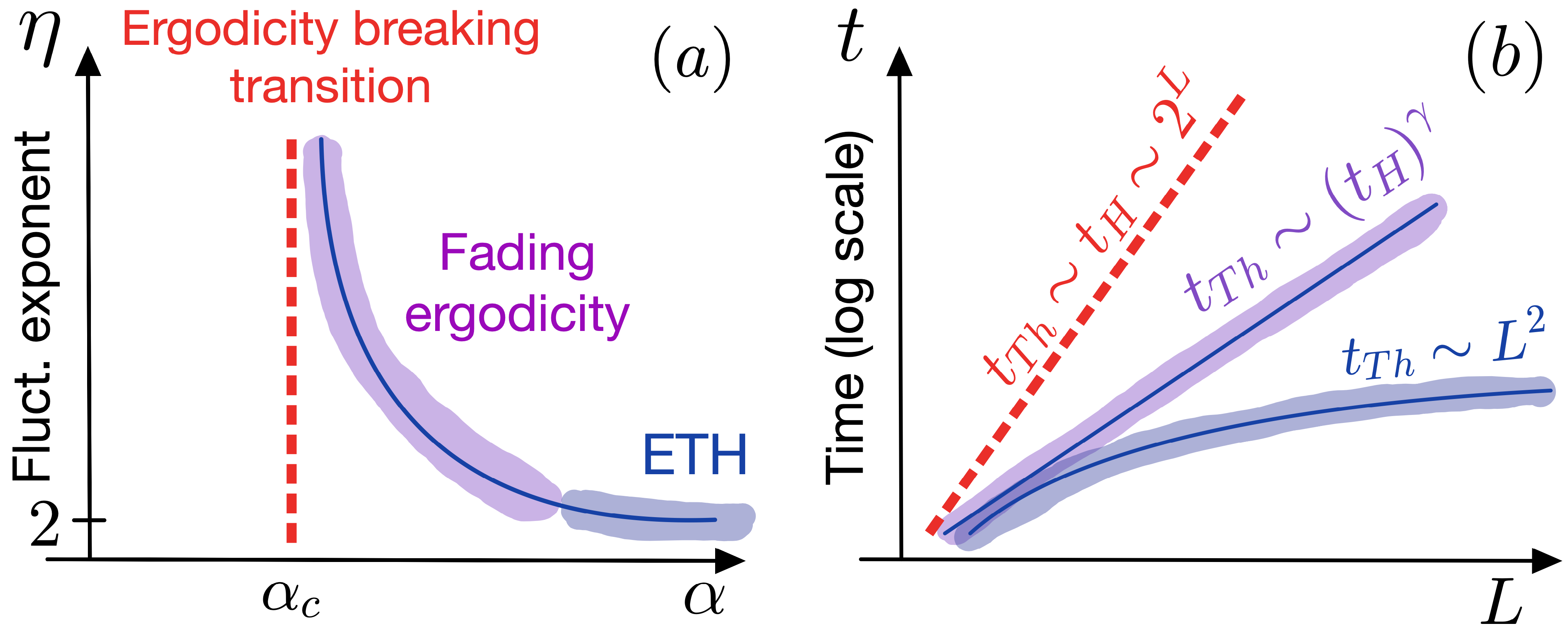
Figure 1: Sketch of the fading ergodicity scenario. (a) Divergence of the fluctuation exponent $\eta$, see Eq. (3), as a function of the control parameter $\alpha$, when approaching the ergodicity breaking transition point at $\alpha=\alpha_{c}$. (b) While the Thouless time $t_{\rm Th}$ is proportional to the Heisenberg time $t_{H}$ at the transition point ($t_{\rm Th}\sim t_{H}$), and it is much smaller than $t_{H}$ in the conventional ETH regime (e.g., $t_{\rm Th}\sim L^{2}$), it scales as $t_{\rm Th}\sim(t_{H})^{\gamma}$, with $0<\gamma<1$, when the boundary of ergodicity is approached.

Softening of ETH at small energies. We now present an argument supporting Eq. (3), i.e., a scenario that naturally interpolates between the conventional ETH ($\eta=2$) and its breakdown in the non-ergodic limit ($\eta\to\infty$). The argument is based on the $L$-dependence of the off-diagonal matrix elements at low $\omega$ for the targeted observable $\hat{O}$. For simplicity, we model the coarse-grained off-diagonal matrix elements at low $\omega$ with a Lorentzian function. This specific functional form is not crucial for the derivation of our main result, however, since we are approaching the ergodicity boundary from the ergodic side, it is important that the function is a constant in the $\omega\to 0$ limit. We consider

$$\overline{|O_{nm}|^{2}}\rho=\frac{\Gamma}{\Gamma^{2}+\omega^{2}}\;,$$ (4)

where for simplicity we omit the energy dependence of $\rho$. The width of the function $\Gamma$ is a characteristic low-energy scale that we name the Thouless energy. We refer to low-$\omega$ off-diagonal matrix elements as those that belong to the interval $\Delta<\omega<\Gamma$, where $\Delta\propto 1/\rho$ is the many-body mean level spacing, i.e., the Heisenberg energy.

Importantly, the Thouless energy $\Gamma$ depends on $L$ in most physical systems. Consequently, also the scaled off-diagonal matrix elements $\overline{|O_{nm}|^{2}}\rho$ are expected to depend on $L$. This is a known property, which is usually interpreted via the $L$-dependence of $f(\bar{E},\omega)$, see Eq. (1), at $\omega\ll\Gamma$ dalessio_kafri_16; luitz_barlev_16; brenes_leblond_20; richter_dymarsky_20; schoenle_jansen_21; wang_lamann_22; Sugimoto2022; balachandran_santos_23. However, in many cases this $L$-dependence is polynomial, and it is hence subleading when compared to the exponentially increasing $\rho$.

Equation (4) suggests that one may restore scale invariance by expressing the matrix elements as a function of $\omega/\Gamma$, giving rise to the following scale-invariant form:

$$\overline{|O_{nm}|^{2}}\rho\Gamma=\frac{1}{1+(\omega/\Gamma)^{2}}.$$ (5)

As a consequence, the low-energy offdiagonals at $\omega\ll\Gamma$ scale as

$$\overline{|O_{nm}|^{2}}\propto\frac{1}{\rho\Gamma}\approx\frac{\Delta}{\Gamma}\;.$$ (6)

Equation (6) is the main result of this study: whenever the Thouless energy increases as $\Gamma\propto\Delta^{\zeta}$, with $0<\zeta<1$, the system is still ergodic but the ETH does not hold in the conventional way (1). In particular, the fluctuations of the matrix elements are softened according to Eq. (3) as $\eta=2/(1-\zeta)>2$, i.e., $\eta$ diverges at the ergodicity breaking transition at which the Thouless energy scales as the Heisenberg energy, $\Gamma\propto\Delta$.

The physical picture that emerges from our study is the suppression of fluctuations of the low-$\omega$ off-diagonal matrix elements, as well as the diagonal matrix elements, which can be interpreted as the accumulation of spectral weight in the ergodic system at $\omega\ll\Gamma$. In contrast, the sum rule for the matrix elements from Eq. (2) then suggests the depletion of the spectral weight at $\omega\gg\Gamma$. We expect this phenomenology to be a generic feature of finite ergodic systems that approach the boundaries of ergodicity, irrespective of whether the ergodicity breaking transition becomes a true phase transition in the thermodynamic limit, or the non-ergodic regime ultimately becomes a singular point in the parameter space.

Example: Quantum sun model. We now present analytical and numerical evidence that supports the above scenario in a toy model that hosts an ergodicity breaking phase transition in the thermodynamic limit, i.e., the quantum sun model of the avalanche theory deroeck_huveneers_17; luitz_huveneers_17; suntajs_vidmar_22. The Hamiltonian is defined as

$$\hat{H}=\hat{H}_{\rm dot}+\sum_{j=1}^{L}\alpha^{u_{j}}\hat{S}_{n_{j}}^{x}\hat{S}_{j}^{x}+\sum_{j=1}^{L}h_{j}\hat{S}_{j}^{z},$$ (7)

where $\hat{H}_{\rm dot}$ is a $2^{N}\times 2^{N}$ random matrix drawn from the Gaussian orthogonal ensemble (GOE) describing all-to-all interacting particles within an ergodic quantum dot (we set $N=3$). The second term defines the coupling between a spin $j$ outside the dot ($j=1,...,L)$ and a randomly selected spin $n_{j}$ within the dot, with $\alpha$ acting as the tuning parameter of the ergodicity breaking phase transition, and $u_{j}\propto j$. Details of the model implementation and the choice of model parameters are given in SM.

A convenient aspect of the quantum sun model is that it allows for using accurate closed-form expressions for the Thouless and Heisenberg energies. The Thouless energy on the ergodic side can be well approximated as suntajs_vidmar_22

$$\Gamma\propto e^{-\ln\left(\frac{1}{\alpha^{2}}\right)L}\;,$$ (8)

while the Heisenberg energy scales, up to subleading corrections, as $\Delta\propto 2^{-L}=\exp{-L\ln{\quantity(1/\tilde{\alpha}_{c}^{2})}}$, where $\tilde{\alpha}_{c}=1/\sqrt{2}$ is the critical point derived within the avalanche theory deroeck_huveneers_17; suntajs_hopjan_24. Hence, using Eq. (6), one can estimate the scaling of the low-$\omega$ off-diagonal matrix elements as

$$\overline{|O_{nm}|^{2}}\propto e^{-\ln\left(\frac{\alpha^{2}}{\tilde{\alpha}_{c}^{2}}\right)L}\;,$$ (9)

which leads to a closed-form expression for the divergence of $\eta$ from Eq. (3),

$$\eta^{*}=2\left(1-\frac{\ln\alpha}{\ln\tilde{\alpha}_{c}}\right)^{-1}\;,$$ (10)

in the ergodic phase at $\tilde{\alpha}_{c}\leq\alpha\leq 1$. While $\tilde{\alpha}_{c}=1/\sqrt{2}\approx 0.707$ provides a reasonably accurate prediction of the transition point, in what follows we refer to the numerically extracted transition point as $\alpha_{c}$, and the difference between $\tilde{\alpha}_{c}$ and $\alpha_{c}$ is of the order of a few percents.

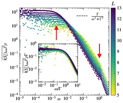
Figure 2: Coarse-grained off-diagonal matrix elements of $\overline{|(S_{L}^{z})_{nm}|^{2}}$ at $\alpha=0.86$ and different $L$. Main panel: $\overline{|(S_{L}^{z})_{nm}|^{2}}\rho$ vs $\omega$, where the density of states $\rho\propto 2^{L}$ is obtained from a small energy window in the middle of the spectrum. Dashed lines are fits to the Lorentzian function (4), from which we extract $\Gamma$. The red arrows highlight the weight accumulation (depletion) at low (high) $\omega$. Inset: $\overline{|(S_{L}^{z})_{nm}|^{2}}\rho\Gamma$ vs $\omega/\Gamma$.

In Fig. 2 and 3 we numerically test the above predictions. We focus on the observable $\hat{O}=\hat{S}_{L}^{z}$, i.e., the projection of the most weakly coupled spin on the z-axis. The physical motivation for selecting this observable is based on understanding that observables, which measure properties of spins that are most weakly coupled to the ergodic quantum dot, are most sensitive to ergodicity breaking suntajs_hopjan_24. Results for other observables are shown in SM.

In Fig. 2, we show the $\omega$-dependence of the coarse-grained off-diagonal matrix elements $\overline{|(S_{L}^{z})_{nm}|^{2}}$, where $(S_{L}^{z})_{nm}\equiv\langle n|\hat{S}_{L}^{z}|m\rangle$ and the coarse graining is carried out over a narrow window above the target $\omega$. The scaled matrix elements $\overline{|(S_{L}^{z})_{nm}|^{2}}\rho$ vs $\omega$ exhibit accumulation of spectral weight at low $\omega$ and its depletion at large $\omega$, see the arrows in the main panel of Fig. 2. Remarkably, the results in Fig. 2 are shown for $\alpha=0.86$, for which the nearest level-spacing statistics complies with the GOE predictions SM. This suggests that the softening of the fluctuations of the matrix elements emerges while the short-range statistics are still GOE-like. Another perspective on the softening of the low-$\omega$ matrix elements is shown in the inset of Fig. 2, in which we show the scaled matrix elements $\overline{|(S_{L}^{z})_{nm}|^{2}}\rho\Gamma$ vs $\omega/\Gamma$, exhibiting a reasonably good collapse of the results for all system sizes under investigation.

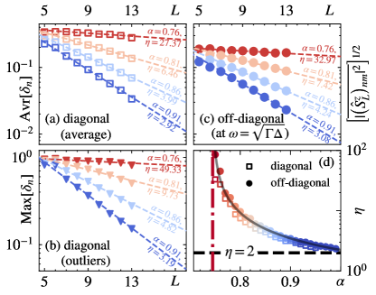
Figure 3: Scaling of fluctuations of matrix elements. (a), (b) Eigenstate-to-eigenstate fluctuations of the diagonal matrix elements, $\delta_{n}\equiv|(\hat{S}^{z}_{L})_{n+1}-(\hat{S}^{z}_{L})_{n}|$. We show the average and the maximal outliers in (a) and (b), respectively, see also SM. (c) Low-$\omega$ off-diagonal matrix elements, taken from a narrow energy window around the target $\omega=\sqrt{\Gamma\Delta}$. Dashed lines in (a)-(c) are the two-parameter fits of the function $a_{0}2^{-L/\eta}$ with the values of $\eta$ shown next to them. (d) Fluctuation exponents $\eta$ from Eq. (3) as a function of $\alpha$. The solid line is a fit of $b_{0}\eta^{*}$ to the results for the off-diagonal matrix elements, where $b_{0}=1.12$ is the fitting parameter and $\eta^{*}$ is the function from Eq. (10), in which $\tilde{\alpha}_{c}$ is replaced by a fitting parameter $\alpha_{c}$. We get $\alpha_{c}=0.745$, see the vertical dashed-dotted line, which is very close to the values of transition point obtained from other indicators such as the average gap ratio SM.

A quantitative analysis of the fluctuations of the matrix elements in carried out in Fig. 3. We study the average eigenstate-to-eigenstate fluctuations of the diagonal matrix elements, see Fig. 3(a), and the fluctuations of the low-$\omega$ off-diagonal matrix elements measured at $\omega=\sqrt{\Delta\Gamma}$, see Fig. 3(c). They both exhibit a fast decay deep in the ergodic regime (at $\alpha$ close to $\alpha=1$), while the decay becomes much slower when the ergodicity breaking transition point is approached, $\alpha\to\alpha_{c}$. The extracted fluctuation exponents $\eta$ as functions of $\alpha$ are shown as symbols in Fig. 3(d). They behave very similarly for the diagonal and the low-$\omega$ off-diagonal matrix elements, and remarkably, are well described by the solid line that corresponds to the analytical prediction from Eq. (10). Moreover, Fig. 3(b) shows that even the maximal outliers of the diagonal matrix elements decay to zero with increasing $L$. This property suggest that the system is still ergodic, and makes a clear distinction to non-ergodic systems such as integrable interacting systems in which the maximal outliers do not decay with system size biroli_lauchli_10; leblond_mallayya_19; lydzba_mierzejewski_23. In SM we also show the distributions of the matrix elements. They appear to be close to a normal distribution in nearly entire ergodic phase.

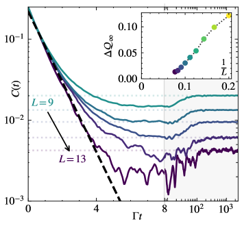
Figure 4: Time evolution of the autocorrelation function $C(t)=\langle\hat{S}_{L}^{z}(t)\hat{S}_{L}^{z}(0)\rangle$ at $\alpha=0.86$ and different system sizes $L$, as a function of scaled time $\Gamma t$. Dashed line denotes the exponential decay $\propto e^{-\Gamma t}$, and horizontal dotted lines represent the long-time average $C_{\infty}$. Inset: difference $\Delta\mathcal{Q}_{\infty}$ between the long-time average of the observable $\mathcal{Q}(t)=\langle\hat{S}_{L}^{z}(t)\rangle$ after a quantum quench and the microcanonical ensemble prediction, vs $1/L$. See SM for details about the quench protocols.

Finally, we demonstrate the emergence of ergodicity from the dynamical perspective. In Fig. 4 we study the dynamics of two related quantities, the autocorrelation function $C(t)=\langle\hat{S}_{L}^{z}(t)\hat{S}_{L}^{z}(0)\rangle$ and the observable $\mathcal{Q}(t)=\langle\hat{S}_{L}^{z}(t)\rangle$ after a quantum quench from initial product states, while in SM we show the growth of the entanglement entropy towards the maximal value. The autocorrelation function $C(t)$ shown in the main panel of Fig. 4 exhibits an initial exponential decay, followed by an approach at long times to the steady-state value that vanishes with increasing the system size $L$. In the inset of Fig. 4, we compare the long-time value of $\mathcal{Q}(t)$ after a quantum quench to the microcanonical ensemble prediction, and we show that their difference vanishes as $L\to\infty$. In SM we also demonstrate that the temporal fluctuations above the long-time average vanish in the thermodynamic limit. Still, the finite-size scaling of temporal fluctuations exhibit softening that resembles the softening of the fluctuations exponent $\eta$ shown in Fig. 3(d). Since the temporal fluctuations are upper-bounded by the decay of the maximal off-diagonal matrix element dalessio_kafri_16, they represent an indicator to detect fingerprints of fading ergodicity based on quantum dynamics.

Conclusions. Historically, the ETH ansatz for the matrix elements of observables was introduced by defining the smooth functions $O(\bar{E})$ and $f(\bar{E},\omega)$ as a refinement beyond the RMT behavior srednicki_99; dalessio_kafri_16. The physical significance of this refinement was to properly describe the energy dependence of matrix elements in physical systems that exhibit thermalization. Recent work has also explored refinements of ETH due to correlations between the matrix elements foini_kurchan_19, which give rise, among others, to nontrivial dynamics of four-point correlation functions foini_kurchan_19; chan_deluca_19; murthy_srednicki_19b; pappalardi_foini_22; Dymarsky2022. In this work we introduce a new modification of the RMT behavior that concerns the softening of the fluctuations of matrix elements. We refer to this phenomenon as fading ergodicity, which is characterized by the breakdown of the conventional ETH. Its physical significance is to allow for detecting boundaries of ergodicity. In case of a well-defined ergodicity breaking phase transition in the thermodynamic limit, fading ergodicity can be considered as a precursor of the transition point at which the ETH ceases to be valid.

We provided analytical arguments and showed numerical evidence in the quantum sun model of ergodicity breaking transitions that the breakdown of conventional ETH is not associated to the breakdown of GOE-like spectral statistics, since the former occurs when later is still valid. Yet, we argued that the unconventional form of fluctuations of matrix elements (i.e., the softening of fluctuations) is still consistent with thermalization of observables. We expect this feature to be generic and to have applications in different types of ergodicity breaking phenomena.

S1 Matrix elements of observables

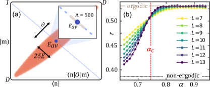
Figure S1: (a) A sketch of matrix elements $\langle n|O|m\rangle$ studied in this work. Main panel: The shaded region represents the off-diagonal matrix elements used to extract their $\omega$-dependence. Inset: diagonal matrix elements in the middle of the spectrum, around the mean energy $E_{\rm av}$. (b) Average gap ratio $r$ vs $\alpha$, for different system sizes $L$. Vertical dashed line denotes the transition point $\alpha_{c}$, extracted in Fig. 3(d) of the main text, while the horizontal solid and dotted lines show the ergodic and non-ergodic value respectively.

An operator matrix, expressed in the basis of the Hamiltonian eigenstates, takes the form

$$\hat{O}=\sum_{n,m=1}^{\cal D}O_{nm}|n\rangle\langle m|\;,$$ (S1)

where $O_{nm}\equiv\langle n|\hat{O}|m\rangle$, $O_{n}\equiv O_{nn}$, and the states $|n\rangle$ and $|m\rangle$ denote the Hamiltonian eigenstates with corresponding eigenenergies $E_{n}$, satisfying $\hat{H}|n\rangle=E_{n}|n\rangle$. When studying ETH, it is important to properly normalize the observables mierzejewski_vidmar_20; leblond_mallayya_19; lydzba_swietek_24. This is achieved, for traceless observables considered here, via the sum rule from Eq. (2) in the main text. The latter can be interpreted as requiring the Hilbert-Schmidt norm of the operator (divided by the Hilbert space dimension ${\cal D}$) to equal one.

To study the diagonal matrix elements, we restrict the analysis to the subset of $\Lambda=500$ eigenstates around the mean energy $E_{\rm av}=\Tr\{\hat{H}\}/\mathcal{D}$, as sketched in the inset of Fig. S1(a). For the off-diagonal matrix elements we restrict the analysis to the eigenstates within a narrow energy window $|(E_{n}+E_{m})/2-E_{\rm target}|<\delta\bar{E}$ around the target energy $E_{\rm target}$, as illustrated by the shaded region in Fig. S1(a). We set the target energy $E_{\rm target}=E_{\rm av}$ and the energy width $\delta\bar{E}/L=10^{-3}$, such that the ratio of the microcanonical window to the bandwidth is $O(1)$. In Fig. 2 of the main text and in Figs. S2(a)-S2(c) we study the coarse-grained off-diagonal matrix elements $\overline{|O_{nm}|^{2}}$ as a function of their energy difference $\omega=E_{n}-E_{m}$. For each bin, we obtain the values of $\overline{|O_{nm}|^{2}}$ by averaging over a narrow interval around the target $\omega$. We use a fixed number of bins, which are evenly spaced on a logarithmic scale ranging from the mean level spacing $\omega\sim\Delta$ (specifically, we take $\omega=\omega_{\rm min}=0.1/{\cal D}$) to $\omega=\omega_{\rm max}$, with $\omega_{\rm max}$ being the bandwidth of the model. The number of bins is of the order of hundred and it increases slightly with the system size.

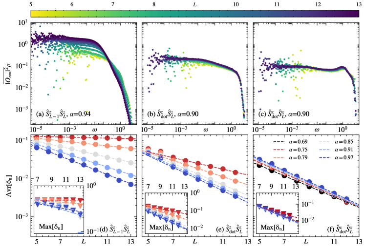
Figure S2: (a)-(c) Coarse-grained off-diagonal matrix elements $\overline{|O_{nm}|^{2}}\rho$ vs $\omega$, where the density of states $\rho$ is obtained from a small energy window in the middle of the spectrum. Results are shown for the observables $\hat{S}^{z}_{L-1}\hat{S}^{z}_{L}$, $\hat{S}^{z}_{\rm dot}\hat{S}^{z}_{L}$, and $\hat{S}^{x}_{\rm dot}\hat{S}^{x}_{L}$, respectively, for different $L$. (d)-(f) Eigenstate-to-eigenstate fluctuations of the diagonal matrix elements, $\delta_{n}\equiv|O_{n+1}-O_{n}|$, vs $L$, for the same observables as shown in (a)-(c), respectively. We show the average values of $\delta_{n}$ in the main panels and the maximal outliers in the insets. Dashed lines are two-parameter fits to the function $a_{0}2^{-L/\eta}$.

S2 Quantum sun model

The quantum sun model, defined in Eq. (7) of the main text, represents a system of $N+L$ spin-1/2 particles deroeck_huveneers_17; luitz_huveneers_17; suntajs_vidmar_22; suntajs_hopjan_24. $N$ particles form an ergodic quantum dot with all-to-all random interactions (we fix $N=3$ throughout the study), while $L$ particles reside outside the dot. The total Hilbert space dimension is ${\cal D}=2^{N+L}$. The interactions of spins within the dot are described by a $2^{N}\times 2^{N}$ random matrix taken from a Gaussian orthogonal ensemble (GOE) suntajs_hopjan_24,

$$\hat{H}_{\rm dot}=\frac{1}{\sqrt{2^{N}+1}}R\;,$$ (S2)

where $R=(A+A^{T})/\sqrt{2}$ and the matrix elements $A_{i,j}=\mathcal{N}(0,1)$ are sampled from a normal distribution with zero mean and unit variance. Each of the spins outside the dot is coupled to a single randomly selected spin within the dot with a strength of $\alpha^{u_{j}}$, where $\alpha$ is the parameter that drives the ergodicity breaking transition, and $u_{j}$ (with $j=1,2,...,L$) are drawn from a uniform distribution, $u_{j}\in[(j-1)-0.2,(j-1)+0.2]$, except for $j=1$ when $u_{1}=0$. The spins outside the dot are also subject to random magnetic fields $h_{j}$, which are drawn from a uniform distribution, $h_{j}\in[0.5,1.5]$. The diagonal and off-diagonal matrix elements of observables, discussed in Sec. S1, are collected with $N_{\rm samples}=2000$ for $11\geq L\geq 5$ and $N_{\rm samples}=874,89$ for $L=12,13$, respectively.

The analytical prediction for the ergodicity breaking transition point, based on the hybridization condition deroeck_huveneers_17, is $\tilde{\alpha}_{c}=1/\sqrt{2}\approx 0.707$. The exact numerical calculations of different ergodicity indicators predict the value of the transition point $\alpha_{c}$ that is close to $\tilde{\alpha}_{c}$. For the model parameters considered here the transition point is estimated to be in the interval $\tilde{\alpha}_{c}\lesssim\alpha_{c}\lesssim 0.75$ suntajs_hopjan_24. In particular, in Fig. 3(d) of the main text we obtained $\alpha_{c}\approx 0.74$ using the divergence of the fluctuation exponent $\eta$ as the transition indicator. In Fig. S1(b) we study the standard transition indicator, namely, the average nearest level spacing ratio $r$, shortly the average gap ratio. Introducing $r_{n}={\rm min}\{\delta E_{n},\delta E_{n-1}\}/{\rm max}\{\delta E_{n},\delta E_{n-1}\}$, where $\delta E_{n}=E_{n+1}-E_{n}$ is the level spacing between the levels $n$ and $n+1$, we obtain the average gap ratio $r$ by averaging $r_{n}$ over 500 eigenstates near the center of the spectrum and over different Hamiltonian realizations. Results in Fig. S1(b) suggest that the scale invariant point of $r$ vs $\alpha$, which denotes the ergodicity breaking transition point suntajs_hopjan_24, is quantitatively very close to $\alpha_{c}\approx 0.74$ predicted by the analysis of $\eta$ in Fig. 3(d).

S3 Choice of observables

The analysis in the main text focuses on the observable $\hat{S}_{L}^{z}$, where $\hat{S}^{z}_{j}=\hat{\sigma}^{z}_{j}/2$ and $\hat{\sigma}_{j}^{z}$ is a Pauli operator acting on a spin labeled by index $j$. Here we extend the analysis to two-point spin correlations $\hat{S}^{z}_{L-1}\hat{S}^{z}_{L}$, $\hat{S}^{z}_{\rm dot}\hat{S}^{z}_{L}$ and $\hat{S}^{x}_{\rm dot}\hat{S}^{x}_{L}$, where $\hat{S}^{z}_{\rm dot}$ and $\hat{S}^{x}_{\rm dot}$ act on a randomly selected spin within the dot.

The results in Fig. S2 show how susceptible are the fluctuations of observable matrix elements to the proximity of the ergodicity breaking transition. The behavior of the matrix elements of $\hat{S}^{z}_{L-1}\hat{S}^{z}_{L}$ is similar to the behavior of $\hat{S}_{L}^{z}$ studied in the main text: the spectral weight of the off-diagonal matrix elements is accumulating at low $\omega$ [cf. Fig. S2(a)] and the fluctuations of the diagonal matrix elements gradually soften when $\alpha$ approaches the transition point [cf. Fig. S2(d)]. The common property of the observables $\hat{S}_{L}^{z}$ and $\hat{S}^{z}_{L-1}\hat{S}^{z}_{L}$ is that they measure properties of spins that are at large distance from the ergodic quantum dot, and hence they exhibit the weakest coupling in the system.

On the other hand, both observables $\hat{S}^{z}_{\rm dot}\hat{S}^{z}_{L}$ and $\hat{S}^{x}_{\rm dot}\hat{S}^{x}_{L}$ include the operator within the ergodic quantum dot. This property makes the proximity of the ergodicity breaking transition less apparent, as seen in Figs. S2(b)-S2(c) and S2(e)-S2(f). For the matrix elements of $\hat{S}^{z}_{\rm dot}\hat{S}^{z}_{L}$, the softening of fluctuations is mild but still noticeable [cf. Figs. S2(b) and S2(e)], while for $\hat{S}^{x}_{\rm dot}\hat{S}^{x}_{L}$, there is no signature of softening [cf. Figs. S2(c) and S2(f)]. The latter is a consequence of the nonergodic phase being localized in the computational basis suntajs_hopjan_24, which is the eigenstate basis of the $\hat{S}^{z}$ operator. For the observable $\hat{S}^{x}_{\rm dot}\hat{S}^{x}_{L}$, we find that the conventional ETH appears to be valid even on the non-ergodic side of the transition. Hence the matrix elements of the observable $\hat{S}^{x}_{\rm dot}\hat{S}^{x}_{L}$ are not expected to contain any special signature of the fading ergodicity regime.

S4 Distribution of matrix elements

The distributions of matrix elements of observables that comply with the conventional ETH are to a good approximation described by a normal distribution (with certain deviations that are manifested in finite systems luitz_barlev_16; wang_wang_18; haque_mcclarty_2022; kliczkowski_swietek_23). We here study the distributions of the matrix elements of observables in the ergodic regime where the conventional ETH is not valid. We ask the question to what degree are the distributions in this regime described by a normal distribution.

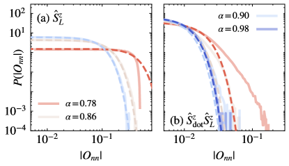
Figure S3: PDFs $P(|O_{nn}|)$ of the diagonal matrix elements of observables: (a) $\hat{O}=\hat{S}^{z}_{L}$ and (b) $\hat{O}=\hat{S}^{z}_{\rm dot}\hat{S}^{z}_{L}$, for the system size $L=12$. Dashed lines indicate fits to the Gaussian PDF from Eq. (S3). We numerically subtract the smooth structure function $O(\bar{E})$ to study the distribution of fluctuations.

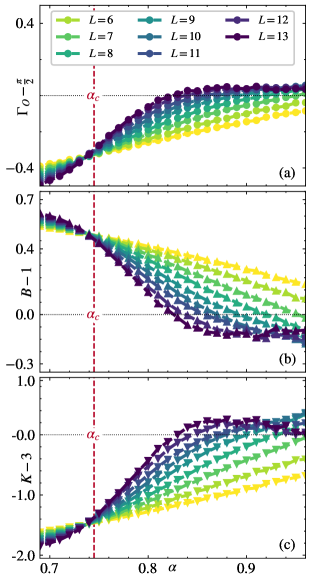
Figure S4: Measures of gaussianity for the diagonal matrix elements of $\hat{S}_{L}^{z}$ vs $\alpha$, for different system sizes $L$. (a) The normalized variance $\Gamma_{O}-\pi/2$ from Eq. (S4), (b) the Binder cumulant $B-1$ from Eq. (S5), and (c) the Kurtosis $K-3$ from Eq. (S6). Horizontal dotted lines are the results for the Gaussian PDF. Vertical dashed lines denote the transition point $\alpha_{c}$ obtained from Fig. 3(d) in the main text.

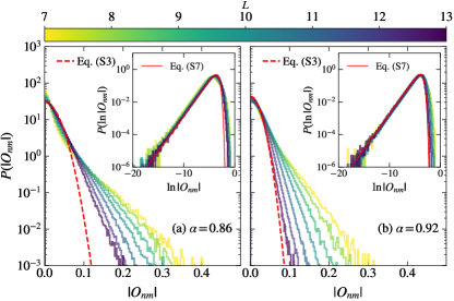
Figure S5: PDFs of off-diagonal matrix elements of the observable $\hat{O}=\hat{S}_{L}^{z}$, studied in the energy interval $\omega<100\Delta$, for (a) $\alpha=0.86$ and (b) $\alpha=0.92$. Main panels: $P(|O_{nm}|)$ vs $|O_{nm}|$. Dashed lines are the fits of the Gaussian PDF from Eq. (S3) to the largest system size. Insets: $P(\ln|O_{nm}|)$ vs $\ln|O_{nm}|$. Solid lines are the fits of the corresponding Gaussian PDF from Eq. (S7) using the same variance.

Figure S3 shows the distributions of the absolute values of diagonal matrix elements of observables $\hat{S}_{L}^{z}$ and $\hat{S}_{\rm dot}^{z}\hat{S}^{z}_{L}$, for a fixed system size and for different values of $\alpha$. Their main feature is that the distribution broadens upon decreasing $\alpha$, which is consistent with the softening of fluctuations in the regime of fading ergodicity.

The dashed lines in Fig. S3 represent the Gaussian probability density functions (PDFs). Given a positive random variable $z$, the corresponding Gaussian PDF is given by

$$\bar{P}(z)=\frac{2}{\sqrt{2\pi\sigma^{2}}}\exp{-\frac{z^{2}}{2\sigma^{2}}}\;,$$ (S3)

where a prefactor 2 appears in the numerator because we study the distribution of absolute values kliczkowski_swietek_23.

While the Gaussian PDFs in Fig. S3 provide accurate descriptions for the numerical distributions at large $\alpha$, they also exhibit deviations at lower $\alpha$ in the tails of the distributions. To quantify the deviations from the Gaussian PDF as functions of both $\alpha$ and $L$, we compute the normalized variance leblond_mallayya_19

$$\Gamma_{O}=\frac{\expectationvalue{z^{2}}}{\expectationvalue{z}^{2}}\;,$$ (S4)

which yields $\Gamma_{O}=\pi/2$ for a Gaussian PDF from Eq. (S3). We complement this measure by computing the Binder cumulant

$$B=\frac{\expectationvalue{z^{4}}}{3\expectationvalue{z^{2}}^{2}}\;,$$ (S5)

which yields $B=1$ for the Gaussian PDF, and the Kurtosis

$$K=\frac{\expectationvalue{(z-\expectationvalue{z})^{4}}}{\expectationvalue{(z-\expectationvalue{z})^{2}}^{2}}\;,$$ (S6)

which yields $K=3$ for the Gaussian PDF.

Figure S4 shows the dependence of the gaussianity measures from Eqs. (S4)-(S6) on $\alpha$, for the observable $\hat{S}_{L}^{z}$ and different system sizes $L$. We observe that the PDFs are indeed close to a Gaussian PDF at large $\alpha$, and notable deviations occur when the transition point is approached. However, the dependence on system size shares certain similarities with other ergodicity measures such as the average gap ratio $r$ studied in Fig. S1(b). This suggests a possibility that in the thermodynamic limit $L\to\infty$, the PDFs are close to Gaussian in the entire ergodic phase. The vertical dashed line in Fig. S4 represents the critical value $\alpha_{c}$ obtained by fitting the divergence of the fluctuation exponent $\eta$ in Fig. 3 using Eq. (10). Notably, all the gaussianity measures studied in Fig. S4 exhibit a scale invariant point that is very close to the extracted value of $\alpha_{c}$ from Fig. 3.

In Fig. S5 we also study the distributions of the off-diagonal matrix elements at fixed $\alpha$ and different system sizes $L$. The dashed line, which is the prediction of the Gaussian PDF from Eq. (S3) for the larger system size, exhibits a good agreement close the peak of the PDFs, while deviations can be observed in the tails of the distributions. In the insets of Fig. S5, we also consider the distribution of $\ln{\absolutevalue{O_{mn}}}$. For a random variable $x=\ln{z}$, where $z$ is distributed according to Eq. (S3), its distribution [shown as solid lines in the insets of Fig. S5] takes the form

$$\tilde{P}(x)=\frac{2e^{x}}{\sqrt{2\pi\sigma^{2}}}\exp{-\frac{e^{2x}}{2\sigma^{2}}}\;.$$ (S7)

The results from the insets of Fig. S5 reinforce the observation from the main panels that the deviations from the Gaussian PDF occur mostly in the tails, i.e., for large values of matrix elements. The deviations are larger in Fig. S5(a) [at $\alpha=0.86$] than in Fig. S5(b) [at $\alpha=0.92$], suggesting similar finite-size phenomenology as observed in Fig. S4 for the diagonal matrix elements.

S5 Quantum dynamics of observables

We now focus on ergodicity through the lens of quantum dynamics. Our goal is to study the dynamics of the expectation value of observable $\hat{S}_{L}^{z}$ after a quantum quench,

$$\mathcal{Q}(t)=\langle\psi_{0}|\hat{S}_{L}^{z}(t)|\psi_{0}\rangle\;.$$ (S8)

We choose the initial state $|\psi_{0}\rangle$ such that we minimize the finite-size effects due to the existence of a many-body mobility edge in the quantum sun model pawlik_sierant_2024. Specifically, for a given Hamiltonian realization, denoted as $\hat{H}^{(\mu)}$, we select a single initial state $|\psi_{0}\rangle$ that is a product state in the computational basis $|i\rangle$ (i.e., an eigenstate of $\hat{S}_{L}^{z}$), such that the energy of this state, $\epsilon_{i}=\langle i|\hat{H}^{(\mu)}|i\rangle$, is closest to the mean energy, $\epsilon_{i}\approx E_{\rm av}^{(\mu)}$. We hence make the expression in Eq. (S8) more precise by explicitly referring to the expectation value of observable for a single Hamiltonian realization $H^{(\mu)}$,

$$\mathcal{Q}(t)^{(\mu)}=\langle\psi_{0}|e^{iH^{(\mu)}t}\hat{S}_{L}^{z}e^{-iH^{(\mu)}t}|\psi_{0}\rangle\;,$$ (S9)

setting $\hbar\equiv 1$. One can rewrite Eq. (S9) as

$$\mathcal{Q}(t)^{(\mu)}=\sum_{n,m}c_{n}^{(\mu)*}c_{m}^{(\mu)}(S_{L}^{z})_{nm}e^{-i(E_{m}^{(\mu)}-E_{n}^{(\mu)})t}\;,$$ (S10)

where the coefficients $\{c_{n}^{(\mu)}\}$ are obtained from the overlaps between the initial state $|\psi_{0}\rangle$ and the Hamiltonian eigenstates, $c_{n}^{(\mu)}=\langle n^{(\mu)}|\psi_{0}\rangle$.

In the long-time limit, the expectation value approaches predictions of the diagonal ensemble (provided the spectrum has no degeneracies) rigol_dunjko_08,

$$\mathcal{Q}_{\infty}^{(\mu)}\equiv\lim_{t\rightarrow\infty}\mathcal{Q}(t)^{(\mu)}=\sum_{n=1}^{\mathcal{D}}|c_{n}^{(\mu)}|^{2}(S_{L}^{z})_{n}\;.$$ (S11)

The expectation values of observables in the diagonal ensemble depend on the initial state of the system via the coefficients $|c_{n}^{(\mu)}|^{2}$. We compare the diagonal ensemble prediction to the microcanonical ensemble average for the same Hamiltonian realization and at the same mean energy $\epsilon_{i}$,

$$\langle\mathcal{Q}^{(\mu)}\rangle_{\rm mic}\equiv\frac{1}{\mathcal{N}_{\epsilon_{i},\Delta_{\epsilon}}}\sum_{|E_{n}^{(\mu)}-\epsilon_{i}|<\Delta_{\epsilon}}(S_{L}^{z})_{n},$$ (S12)

where $\mathcal{N}_{\epsilon_{i},\Delta_{\epsilon}}$ is the normalization factor and the width $\Delta_{\epsilon}$ of the microcanonical ensemble is sufficiently small. In practice, we either set $\Delta_{\epsilon}=5\times 10^{-2}$, or, if the sum in Eq. (S12) contains too few elements (which may be the case for small systems), we select $\mathcal{N}_{\epsilon_{i},\Delta_{\epsilon}}=10$ eigenstates with energies $E_{n}^{(\mu)}$ closest to $\epsilon_{i}$, regardless of $\Delta_{\epsilon}$.

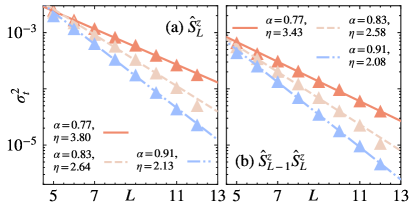
Figure S6: Scaling of the variance of temporal fluctuations $\sigma_{t}^{2}$, see Eq. (S16), vs $L$ for the observables (a) $\hat{S}^{z}_{L}$ and (b) $\hat{S}^{z}_{L-1}\hat{S}^{z}_{L}$. Results are shown for different values of $\alpha$.

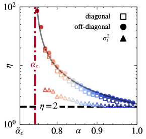
Figure S7: Fluctuation exponents $\eta$ vs $\alpha$. Exponents of the fluctuations of the diagonal (squares) and the low-$\omega$ off-diagonal matrix elements (circles) are identical to those in Fig. 3(d). Exponent of the temporal fluctuations (triangles) are obtained by fitting the function $b_{0}2^{-2L/\eta}$ to the results in Fig. S6.

We define the averaged differences between the diagonal and the microcanonical ensembles as

$$\Delta\mathcal{Q}_{\infty}={\rm Avr}_{\mu}\left\{|\mathcal{Q}_{\infty}^{(\mu)}-\langle\mathcal{Q}^{(\mu)}\rangle_{\rm mic}|\right\}\;,$$ (S13)

where ${\rm Avr}_{\mu}\{...\}$ corresponds to the average over Hamiltonian realizations. We studied $\Delta\mathcal{Q}_{\infty}$ vs $1/L$ in the inset of Fig. 4 of the main text. The averaging over Hamiltonian realizations is carried out over $N_{\rm samples}=500$ for $L\leq 8$, and the number of realizations is then gradually reduced to $N_{\rm samples}=500-100(L-8)$ for $12>L\geq 9$. For $L=12,13$, we use $N_{\rm samples}=25,10$, respectively.

We note that the initial value $\mathcal{Q}(t=0)^{(\mu)}$ at the quantum quench is either $+1/2$ or $-1/2$, depending on the polarization of the spin at $j=L$ in the initial state $|\psi_{0}\rangle$. To study properties of time evolution after averaging over different Hamiltonian realizations, we then define the autocorrelation function

$$C(t)^{(\mu)}\equiv\langle\psi_{0}|\hat{S}_{L}^{z}(t)\hat{S}_{L}^{z}(0)|\psi_{0}\rangle\;,$$ (S14)

which is related to ${\cal Q}(t)^{(\mu)}$ from Eq. (S9) as $C(t)^{(\mu)}=s_{L}^{z}{\cal Q}(t)^{(\mu)}$, with $s_{L}^{z}=\langle\psi_{0}|\hat{S}_{L}^{z}|\psi_{0}\rangle$. In the main panel of Fig. 4 in the main text, we show the average autocorrelation function $C(t)$, which corresponds to $C(t)^{(\mu)}$ from Eq. (S14) averaged over different Hamiltonian realizations.

Another important property of quantum dynamics is whether or not the expectation values of observables equilibrate. To measure that, we define the variance of long-time temporal fluctuations for a given Hamiltonian realization dalessio_kafri_16,

$$\sigma^{2}_{t,\mu}\equiv{\rm Var}_{t}\left\{\tilde{\mathcal{Q}}(t)^{(\mu)}\right\}\;,$$ (S15)

where $\tilde{\mathcal{Q}}(t)^{(\mu)}$ is the expectation value $\mathcal{Q}(t)^{(\mu)}$ [Eq. (S14)] restricted to a time window after the Heisenberg time $t_{\rm H}$. Here, we select the time window $t\in[50t_{H},100t_{H}]$. The corresponding average variance over the Hamiltonian realizations is defined as

$$\sigma^{2}_{t}={\rm Avr}_{\mu}\left\{\sigma^{2}_{t,\mu}\right\}\;.$$ (S16)

One can set an upper bound for $\sigma^{2}_{t,\mu}$ that is given by the decay of the maximal off-diagonal matrix element with system size dalessio_kafri_16. This suggest a relationship between the temporal fluctuations and the fluctuations of matrix elements.

Here we ask whether the breakdown of the conventional ETH in the fading ergodicity regime is also manifested in the scaling of the variance of temporal fluctuations with system size. In Fig. S6 we show $\sigma_{t}^{2}$ vs $L$ for the observables $\hat{S}_{L}^{z}$ and $\hat{S}_{L-1}^{z}\hat{S}_{L}^{z}$, and different values of $\alpha$. We observe that in all cases under consideration, the decay of $\sigma_{t}^{2}$ is exponential with $L$, suggesting equilibration of the system. Moreover, we also observe that the rate of the exponential decay decreases when $\alpha$ approaches the ergodicity breaking transition, which is consistent with the softening of fluctuations of matrix elements. In Fig. S7 we compare the corresponding fluctuation exponents of the temporal fluctuations and the matrix elements fluctuations [as reported in Fig. 3(d)]. The obtained temporal fluctuation exponent is quantitatively smaller than the matrix element fluctuation exponent. However, in all cases, the fluctuation exponent increase when $\alpha$ approaches the transition point $\alpha_{c}$, suggesting that the long-time temporal fluctuations indeed carry information about the softening of the low-$\omega$ off-diagonal matrix elements.

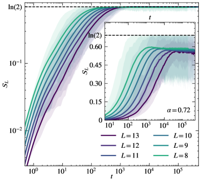
Figure S8: Time evolution of the entanglement entropy ${\cal S}_{L}(t)$, see Eq. (S17), of a single (most weakly coupled) spin. Main panel: $\alpha=0.86>\alpha_{c}$ in the ergodic regime. Inset: $\alpha=0.72<\alpha_{c}$ in the non-ergodic regime. Results are shown for various system sizes $L$. Solid lines represent the averaged entanglement entropy ${\cal S}_{L}(t)$, while the temporal fluctuations in different Hamiltonian realizations are denoted by fading colors.

S6 Growth of entanglement entropy

To complement the analysis, we study the time evolution of the von Neumann entanglement entropy ${\cal S}_{L}(t)$, defined as

$${\cal S}_{L}(t)={\rm Avr}_{\mu}\left\{-\Tr{\hat{\rho}_{L}(t)\ln\hat{\rho}_{L}(t)}\right\}\;,$$ (S17)

where for each Hamiltonian realization $\hat{H}^{(\mu)}$, we choose the same initial state as used in Sec. S5, and we then average the results over different Hamiltonian realizations. In Eq. (S17), $\hat{\rho}_{L}=\Tr_{\rm remain}\{|\psi(t)\rangle\langle\psi(t)|\}$ is the reduced density matrix of the single spin (at $j=L$), obtained by tracing out the remaining spins in the time-evolved state $|\psi(t)\rangle$ at time $t$.

Results shown in Fig. S8 represent the entanglement growth in the ergodic regime (main panel) and in the non-ergodic regime (inset). We observe that in the ergodic regime, the entanglement entropy grows towards its maximum value, ${\cal S}(t\to\infty)\to\ln 2$. The approach towards maximal entanglement entropy is consistent with the ergodic behavior of the system (however, it is not a sufficient condition; see, e.g., Ref. vidmar_hackl_17 for a counter-example). On the other hand, the breakdown of ergodicity is clearly manifested in the inset of Fig. S8 at $\alpha<\alpha_{c}$, in which the entanglement entropy after a long time saturates to a value that is below the maximal value.

References

- (1) O. Bohigas, M. J. Giannoni, and C. Schmit, Characterization of chaotic quantum spectra and universality of level fluctuation laws, Phys. Rev. Lett. 52, 1 (1984).
- (2) G. Casati, F. Valz-Gris, and I. Guarnieri, On the connection between quantization of nonintegrable systems and statistical theory of spectra, Lettere al Nuovo Cimento 28, 279 (1980).
- (3) G. Montambaux, D. Poilblanc, J. Bellissard, and C. Sire, Quantum chaos in spin-fermion models, Phys. Rev. Lett. 70, 497 (1993).
- (4) T. C. Hsu and J. C. Angle‘s d’Auriac, Level repulsion in integrable and almost-integrable quantum spin models, Phys. Rev. B 47, 14291 (1993).
- (5) M. Di Stasio and X. Zotos, Connection between Low Energy Effective Hamiltonians and Energy Level Statistics, Phys. Rev. Lett. 74, 2050 (1995).
- (6) T. Prosen, Ergodic properties of a generic nonintegrable quantum many-body system in the thermodynamic limit, Phys. Rev. E 60, 3949 (1999).
- (7) L. F. Santos, Integrability of a disordered Heisenberg spin-1/2 chain, J. Phys. A. 37, 4723 (2004).
- (8) D. A. Rabson, B. N. Narozhny, and A. J. Millis, Crossover from Poisson to Wigner-Dyson level statistics in spin chains with integrability breaking, Phys. Rev. B 69, 054403 (2004).
- (9) M. Rigol and L. F. Santos, Quantum chaos and thermalization in gapped systems, Phys. Rev. A 82, 011604 (2010).
- (10) I. Bloch, J. Dalibard, and S. Nascimbène, Quantum simulations with ultracold quantum gases, Nature Physics 8, 267 (2012).
- (11) J. M. Deutsch, Quantum statistical mechanics in a closed system, Phys. Rev. A 43, 2046 (1991).
- (12) M. Srednicki, Chaos and quantum thermalization, Phys. Rev. E 50, 888 (1994).
- (13) M. Rigol, V. Dunjko, and M. Olshanii, Thermalization and its mechanism for generic isolated quantum systems, Nature (London) 452, 854 (2008).
- (14) L. D’Alessio, Y. Kafri, A. Polkovnikov, and M. Rigol, From quantum chaos and eigenstate thermalization to statistical mechanics and thermodynamics, Adv. Phys. 65, 239 (2016).
- (15) M. Srednicki, The approach to thermal equilibrium in quantized chaotic systems, J. Phys. A. 32, 1163 (1999).
- (16) G. Biroli, C. Kollath, and A. M. Läuchli, Effect of rare fluctuations on the thermalization of isolated quantum systems, Phys. Rev. Lett. 105, 250401 (2010).
- (17) T. N. Ikeda and M. Ueda, How accurately can the microcanonical ensemble describe small isolated quantum systems?, Phys. Rev. E 92, 020102 (2015).
- (18) V. Alba, Eigenstate thermalization hypothesis and integrability in quantum spin chains, Phys. Rev. B 91, 155123 (2015).
- (19) T. LeBlond, K. Mallayya, L. Vidmar, and M. Rigol, Entanglement and matrix elements of observables in interacting integrable systems, Phys. Rev. E 100, 062134 (2019).
- (20) M. Brenes, T. LeBlond, J. Goold, and M. Rigol, Eigenstate Thermalization in a Locally Perturbed Integrable System, Phys. Rev. Lett. 125, 070605 (2020).
- (21) P. Łydżba, R. Świętek, M. Mierzejewski, M. Rigol, and L. Vidmar, Normal weak eigenstate thermalization, arXiv:2404.02199.
- (22) D. J. Luitz, Long tail distributions near the many-body localization transition, Phys. Rev. B 93, 134201 (2016).
- (23) R. K. Panda, A. Scardicchio, M. Schulz, S. R. Taylor, and M. Žnidarič, Can we study the many-body localisation transition?, EPL 128, 67003 (2019).
- (24) L. A. Colmenarez, P. A. McClarty, M. Haque, and D. J. Luitz, Statistics of correlation functions in the random heisenberg chain, SciPost Physics 7 (2019).
- (25) Á. L. Corps, R. A. Molina, and A. Relaño, Signatures of a critical point in the many-body localization transition, SciPost Phys. 10, 107 (2021).
- (26) N. Shiraishi and T. Mori, Systematic Construction of Counterexamples to the Eigenstate Thermalization Hypothesis, Phys. Rev. Lett. 119, 030601 (2017).
- (27) R. Mondaini, K. Mallayya, L. F. Santos, and M. Rigol, Comment on “Systematic Construction of Counterexamples to the Eigenstate Thermalization Hypothesis”, Phys. Rev. Lett. 121, 038901 (2018).
- (28) M. Serbyn, D. A. Abanin, and Z. Papić, Quantum many-body scars and weak breaking of ergodicity, Nature Physics 17, 675 (2021).
- (29) S. Moudgalya, B. A. Bernevig, and N. Regnault, Quantum many-body scars and Hilbert space fragmentation: a review of exact results, Rep. Prog. Phys. 85, 086501 (2022).
- (30) P. Sala, T. Rakovszky, R. Verresen, M. Knap, and F. Pollmann, Ergodicity Breaking Arising from Hilbert Space Fragmentation in Dipole-Conserving Hamiltonians, Phys. Rev. X 10, 011047 (2020).
- (31) P. Sierant, D. Delande, and J. Zakrzewski, Thouless time analysis of Anderson and many-body localization transitions, Phys. Rev. Lett. 124, 186601 (2020).
- (32) J. Šuntajs, T. Prosen, and L. Vidmar, Spectral properties of three-dimensional Anderson model, Ann. Phys. 435, 168469 (2021).
- (33) J. Šuntajs and L. Vidmar, Ergodicity Breaking Transition in Zero Dimensions, Phys. Rev. Lett. 129, 060602 (2022).
- (34) P. Łydżba, Y. Zhang, M. Rigol, and L. Vidmar, Single-particle eigenstate thermalization in quantum-chaotic quadratic Hamiltonians, Phys. Rev. B 104, 214203 (2021).
- (35) See Supplemental Material for further details on calculations of observables (normalization, choice of observables, their distributions, etc.), the implementation of the quantum sun model, the quantum dynamics of autocorrelation functions, and the growth of entanglement entropies.
- (36) M. Pandey, P. W. Claeys, D. K. Campbell, A. Polkovnikov, and D. Sels, Adiabatic Eigenstate Deformations as a Sensitive Probe for Quantum Chaos, Phys. Rev. X 10, 041017 (2020).
- (37) T. LeBlond, D. Sels, A. Polkovnikov, and M. Rigol, Universality in the onset of quantum chaos in many-body systems, Phys. Rev. B 104, L201117 (2021).
- (38) D. J. Luitz and Y. Bar Lev, Anomalous Thermalization in Ergodic Systems, Phys. Rev. Lett. 117, 170404 (2016).
- (39) J. Richter, A. Dymarsky, R. Steinigeweg, and J. Gemmer, Eigenstate thermalization hypothesis beyond standard indicators: Emergence of random-matrix behavior at small frequencies, Phys. Rev. E 102, 042127 (2020).
- (40) C. Schönle, D. Jansen, F. Heidrich-Meisner, and L. Vidmar, Eigenstate thermalization hypothesis through the lens of autocorrelation functions, Phys. Rev. B 103, 235137 (2021).
- (41) J. Wang, M. H. Lamann, J. Richter, R. Steinigeweg, A. Dymarsky, and J. Gemmer, Eigenstate Thermalization Hypothesis and Its Deviations from Random-Matrix Theory beyond the Thermalization Time, Phys. Rev. Lett. 128, 180601 (2022).
- (42) S. Sugimoto, R. Hamazaki, and M. Ueda, Eigenstate thermalization in long-range interacting systems, Phys. Rev. Lett. 129, 030602 (2022).
- (43) V. Balachandran, L. F. Santos, M. Rigol, and D. Poletti, Slow relaxation of out-of-time-ordered correlators in interacting integrable and nonintegrable spin- xyz chains, Phys. Rev. B 107, 235421 (2023).
- (44) W. De Roeck and F. Huveneers, Stability and instability towards delocalization in many-body localization systems, Phys. Rev. B 95, 155129 (2017).
- (45) D. J. Luitz, F. Huveneers, and W. De Roeck, How a small quantum bath can thermalize long localized chains, Phys. Rev. Lett. 119, 150602 (2017).
- (46) J. Šuntajs, M. Hopjan, W. De Roeck, and L. Vidmar, Similarity between a many-body quantum avalanche model and the ultrametric random matrix model, Phys. Rev. Res. 6, 023030 (2024).
- (47) P. Łydżba, M. Mierzejewski, M. Rigol, and L. Vidmar, Generalized thermalization in quantum-chaotic quadratic hamiltonians, Phys. Rev. Lett. 131, 060401 (2023).
- (48) L. Foini and J. Kurchan, Eigenstate thermalization hypothesis and out of time order correlators, Phys. Rev. E 99, 042139 (2019).
- (49) A. Chan, A. De Luca, and J. T. Chalker, Eigenstate Correlations, Thermalization, and the Butterfly Effect, Phys. Rev. Lett. 122, 220601 (2019).
- (50) C. Murthy and M. Srednicki, Bounds on Chaos from the Eigenstate Thermalization Hypothesis, Phys. Rev. Lett. 123, 230606 (2019).
- (51) S. Pappalardi, L. Foini, and J. Kurchan, Eigenstate thermalization hypothesis and free probability, Phys. Rev. Lett. 129, 170603 (2022).
- (52) A. Dymarsky, Bound on Eigenstate Thermalization from Transport, Phys. Rev. Lett. 128, 190601 (2022).
- (53) www.hpc-rivr.si.
- (54) eurohpc-ju.europa.eu.
- (55) www.izum.si.
- (56) M. Mierzejewski and L. Vidmar, Quantitative Impact of Integrals of Motion on the Eigenstate Thermalization Hypothesis, Phys. Rev. Lett. 124, 040603 (2020).
- (57) J. Wang and W.-G. Wang, Characterization of random features of chaotic eigenfunctions in unperturbed basis, Phys. Rev. E 97, 062219 (2018).
- (58) M. Haque, P. A. McClarty, and I. M. Khaymovich, Entanglement of midspectrum eigenstates of chaotic many-body systems: Reasons for deviation from random ensembles, Phys. Rev. E 105, 014109 (2022).
- (59) M. Kliczkowski, R. Swietek, L. Vidmar, and M. Rigol, Average entanglement entropy of midspectrum eigenstates of quantum-chaotic interacting hamiltonians, Phys. Rev. E 107, 064119 (2023).
- (60) K. Pawlik, P. Sierant, L. Vidmar, and J. Zakrzewski, Many-body mobility edge in quantum sun models, Phys. Rev. B 109, l180201 (2024).
- (61) L. Vidmar, L. Hackl, E. Bianchi, and M. Rigol, Entanglement Entropy of Eigenstates of Quadratic Fermionic Hamiltonians, Phys. Rev. Lett. 119, 020601 (2017).