Entanglement dynamics from universal low-lying modes
Abstract
Information-theoretic quantities such as Renyi entropies show a remarkable universality in their late-time behaviour across a variety of chaotic quantum many-body systems. Understanding how such common features emerge from very different microscopic dynamics remains an important challenge. In this work, we address this question in a class of Brownian models with random time-dependent Hamiltonians and a variety of different microscopic couplings. In any such model, the Lorentzian time-evolution of the -th Renyi entropy can be mapped to evolution by a Euclidean Hamiltonian on 2 copies of the system. We provide evidence that in systems with no symmetries, the low-energy excitations of the Euclidean Hamiltonian are universally given by a gapped quasiparticle-like band. The eigenstates in this band are plane waves of locally dressed domain walls between ferromagnetic ground states associated with two permutations in the symmetric group . These excitations give rise to the membrane picture of entanglement growth, with the membrane tension determined by their dispersion relation. We establish this structure in a variety of cases using analytical perturbative methods and numerical variational techniques, and extract the associated dispersion relations and membrane tensions for the second and third Renyi entropies. For the third Renyi entropy, we argue that phase transitions in the membrane tension as a function of velocity are needed to ensure that physical constraints on the membrane tension are satisfied. Overall, this structure provides an understanding of entanglement dynamics in terms of a universal set of gapped low-lying modes, which may also apply to systems with time-independent Hamiltonians.
I Introduction
Chaotic quantum many-body systems show the universal phenomenon of thermalization. When an arbitrary initial state is evolved to sufficiently late times, it starts to macroscopically resemble a thermal density matrix . This process is independent of most details of the initial state and microscopic dynamics of the system. While thermalization is ubiquitously observed, much remains to be understood both about the mechanism for its robustness across a variety of different microscopic dynamics, and about the effective field-theoretic approaches which can capture its essential aspects. Such an understanding would be valuable not only for quantum many-body physics, but also for understanding the process of black hole formation in quantum gravity, which is an example of thermalization [1, 2].
Thermalization can be probed by using correlation functions of few-body operators in the time-evolved state, as well as information-theoretic quantities such as the Renyi entropies of a subsystem. For an initial state and a unitary time-evolution operator , the time-evolved -th Renyi entropy of a subsystem is given by 111The limit is the von Neumann entropy.
| (1) |
At late times in chaotic systems, saturates to a value that depends only on , reflecting the fact that most details of the initial state are forgotten. For example, if is pure and one of the subsystems is much larger than the other, we expect the general behaviour
| (2) |
The late-time value (2) is intuitively expected based on the behaviour of the Renyi entropies in random pure states [3, 4, 5, 6, 7], and was argued for more systematically in [8].
For the evolution of correlation functions during thermalization, it has long been understood that there are universal behaviours not only in the saturation value, but also in the way in which it is approached at late times. For example, one expects the late-time behaviour of correlation functions of any conserved charge density to be governed by hydrodynamic modes, which depend on the conservation law but not on details of the microscopic dynamics.
A lot of evidence has been gathered for a similar universality in the growth of in chaotic systems before it approaches its late-time value (2), starting with observations of a linear in regime in a variety of chaotic systems [9, 10, 11]. By synthesizing various observations, [12] conjectured a “membrane formula” to describe entanglement growth in general chaotic quantum many-body systems. This formula was found to hold in two very different examples of analytically tractable chaotic quantum many-body systems: random unitary circuits [13, 14, 15, 16], which involve a discrete chaotic evolution with random gates, and holographic conformal field theories [17]. While the result turns out to be the same, the formula is derived in these examples using techniques which are specific to each model.
In this work, we identify the origin of the membrane picture across various examples in a large class of chaotic quantum many-body systems, from a common set of gapped low-lying modes of an effective Hamiltonian. The models we consider have random time-dependent “Brownian” Hamiltonians, with a variety of tunable parameters that allow us to check the robustness of this physical picture. We provide a precise physical interpretation of the “membrane tension” function, the key ingredient of the membrane formula, in terms of the dispersion relation of these modes.
We show that the membrane picture for discrete-time random unitary circuits derived in [14, 15, 12, 16] is a specific case where this structure applies, but in most of this work, the time-evolutions we consider are continuous. Moreover, the same set of modes that we find here can in principle be defined in systems with a fixed time-independent Hamiltonian, and even in continuum quantum field theories such as holographic CFTs. It is tempting to speculate that the same modes also govern the late-time evolution of the Renyi entropies in these contexts, and are entanglement analogs of hydrodynamic modes for correlation functions.
In the rest of the introduction, we first briefly review the membrane picture, and then summarize our methods and results.
I.1 Review of membrane picture
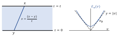
For simplicity, let us state the membrane formula in the case of one spatial dimension. Consider the evolution of the Renyi entropy of a pure or mixed state for the left half-line region ending at . According to the conjecture of [12], this quantity can be expressed as the following minimization problem in any chaotic system. Let us extend the one-dimensional system to a two-dimensional slab, with an auxilliary time axis going from to , as shown in Fig. 1. Then consider all possible lines with different velocities starting at , and extending into the direction. At sufficiently late times, is given by:
| (3) |
Here is the -th Renyi entropy density of the equilibrium state. The function is model-dependent, but is conjectured to always be an even convex function, with a minimum at . It is expected to also universally satisfy the following constraints:
| (4) |
for some velocity , which are necessitated by physical conditions we discuss below. A natural generalization of the formula also holds for multiple intervals and higher dimensions, for details see [12].
To understand the physical consequences of this formula, it is useful to understand its prediction for an initial mixed state with volume law entropy with some coefficient :
| (5) |
where we have assumed that the system has total length , with positions labelled from to . For such states, (3) predicts that
| (6) |
where the entropy growth rate is related to through
| (7) |
The constraints (4) are equivalent to the physical condition that the entropy of the initial equilibrium state should not grow, i.e.,
| (8) |
is the velocity that minimizes (7) for , and due to the fact that , only velocities are physically relevant for the evolution of the entropy.
I.2 Summary of results
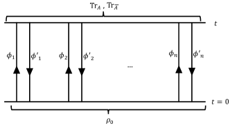
In this work, we will consider a family of “Brownian” time-evolutions in lattice systems, with independent random local Hamiltonians acting at each infinitesimal time-step. Various specific examples of such models have been introduced and studied in the literature over the years [18, 19, 20, 21, 22, 23, 24, 25, 26, 27, 21, 28, 29, 30, 31]. These models are less random than Haar-random unitary circuits, and have various tunable microscopic parameters. The key simplification of such models is that after averaging over randomness, the Lorentzian evolution on copies of the system, which governs the evolution of the -th Renyi entropy, can be replaced with a Euclidean evolution on copies with a non-negative frustration-free Hamiltonian :222In Haar random circuits, this average maps to a classical statistical mechanics model [14, 15]
| (9) |
We will explain the precise setup and derive this mapping from Lorentzian to Euclidean evolution in Sec. II. We will sometimes refer to as the “superhamiltonian” in the discussion below. Due to the mapping in (9), the low-energy properties of the superhamiltonian determine the late-time evolution of quantities such as the -th Renyi entropy. This allows us to use both physical intuition and precise analytical and numerical techniques from the low-energy physics of quantum many-body systems, and apply them to understanding the physics of thermalization.
For , correlation functions of few-body operators in the thermal state or a time-evolved state can be written as transition amplitudes under the evolution operator (9). Some hints that the lessons we learn from Brownian models apply more generally come from Refs. [30, 31], which studied Brownian models with a variety of symmetries, and derived the associated hydrodynamic modes using the low-energy spectrum of . For example, in models with global symmetry, these works used the low-energy gapless modes of to derive diffusive behaviour of two-point functions of the charge density.
The Renyi entropies can be written as transition amplitudes under (9) for . We first show that in general Brownian models with any symmetry, we can use the zero energy eigenstates of to derive a late-time saturation value of consistent with the equilibrium approximation of [8], and in particular with (2). We then specialize to the case of Brownian models with no symmetries, where generically has an -dimensional ground state subspace. The ground state subspace is spanned by states associated with permutations in , which have a product form between different sites of the system:
| (10) |
The precise definition of will be given in Sec. II. We will provide more intuitition for why states associated with permutations should be relevant for the late-time behaviour of the Renyi entropies at the end of the introduction.
In one spatial dimension, we find evidence that the low-energy excitations of in models with no symmetries have the following universal structure. Let us denote the identity permutation in by , and the cyclic permutation which sends to , to , and so on, by . The low-energy eigenstates are well-approximated by plane waves of locally dressed domain walls between the states associated with and . More explicitly, we find that they can be well-approximated as
| (11) |
where is in the thermodynamic limit, and is an arbitrary state in the full Hilbert space on copies of sites from to . We will show that the structure (11) of the eigenstates in the thermodynamic limit leads to the membrane formula (3) for a half-line region. These eigenstates have a gapped dispersion relation , which determines the entanglement growth rate of (6) through the relation
| (12) |
This in turn determines the membrane tension through the inverse of (7). The natural “multiparticle” versions of these single domain wall excitations give rise to the membrane picture for subsystems consisting of one or more intervals.333Note that these effective “particles” which appear in the chaotic systems in this work have an entirely different structure from the quasiparticle picture of Calabrese and Cardy [32]. The latter applies to integrable systems and gives very different results for the evolution of for multiple intervals from the chaotic case [33, 34].
We establish the above universal structure of the low-energy eigenstates of by studying the following cases:
-
1.
We start with the simplest case of a maximally random Brownian Hamiltonian, where the local coupling operators are drawn from the GUE ensemble and the local Hilbert space dimension is large. For the second Renyi entropy in this case, the superhamiltonian is analytically tractable, and allows us to explicitly see that the low-energy eigenstates have the form (11).
-
2.
Next, we consider the second Renyi entropy in the same model at finite local Hilbert space dimension . Since the superhamiltonian is no longer analytically tractable, we use a version of the variational approach used for extracting low-energy excitations of gapped Hamiltonians in [35, 36, 37]. This method allows us to both verify that the eigenstates are well-approximated by (11), and to extract their dispersion relation . In this case, the on-site Hilbert space dimension of the superhamiltonian is sufficiently small that we can also check obtained from the variational method with results from exact diagonalization, finding good agreement.
-
3.
We then turn to the case of the higher Renyi entropies in the same model, in particular focusing on the third Renyi entropy. While we can no longer use exact diagonalization due to the large on-site Hilbert space dimension of the superhamiltonian, we again use the variational approach to check that the low-energy eigenstates have the structure (11), and extract the associated .
-
4.
Finally, we consider the evolution of in a class of Brownian models where the coupling operators are fixed to be those of the mixed field Ising model, and only the coefficients appearing next to the operators have time-dependent randomness. For generic values of the coupling strength, the model is expected to be chaotic, except close to a special integrable point. Consistent with this expectation, we find good evidence for the structure (11) using the variational approach in the general case, and a breakdown of this structure close to the integrable point.
In cases 1, 2, and 4 above, we find that the membrane tensions for the second Renyi entropy resulting from the dispersion relations satisfy (4), or equivalently satisfies (8). The case of the third Renyi entropy from point 3 turns out to be more subtle. The naive growth rate from the dispersion relation of modes (11) appears to be non-zero at . However, we conjecture that the evolution of also receives contributions from a second set of modes besides (11) in this case. We argue that beyond some value of , the naive growth rate should be replaced with the growth rate implied by this second set of modes, which is the same as . In terms of the membrane tension, we find that this single first-order phase transition in leads to two phase transitions in terms of at velocities . We have a first-order phase transition at and a second-order transition at . For , is smaller than , while for , .
While the above discussion of uses an assumption about the existence of the second set of modes which should be more carefully checked in future work, it allows us to propose a form of at finite and general . Hence, we are able to provide a characterization of the phase transitions of in a more general regime than previous discussions in random unitary circuits [16], where evidence for a phase transition was found using expansions for large and large . Our physical picture for the origin of the phase transition appears to be similar to the one in [16].
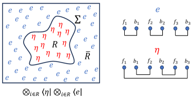
The structure of the modes (11) can be seen as a simple and precise realization of an insight from [38] about the crucial role played by permutations in the late-time evolution of the Renyi entropies. Note that the Lorentzian path integral representation of the quantity , shown schematically in Fig. 2, involves an integrand of the form , where represent the dynamical fields of the theory along forward and backward contours respectively. Ref. [38] noted that we get stationary contributions in this path integral from configurations where each is equal to some for some , as the phase in the exponent cancels. From other configurations, in a chaotic system, we should expect rapidly oscillating contributions that cancel among themselves. Based on this observation, [8] developed a systematic approximation for the saturation value of .
At late times before saturation, it is natural to expect that the dominant configurations should be such that each is locally equal to some for some , but different permutations can appear in different regions. [38] developed a self-consistent numerical scheme based on this idea for evaluating the membrane tension in circuit and Floquet models. The scheme involved a sum over spacetime diagrams, where the contributions from diagrams with large spacetime regions with states orthogonal to the permutation subspace were neglected. In the models considered in this work, we can better understand the suppression of such diagrams due to the high energy of the associated configurations in the Euclidean superhamiltonian. The analog of the summation over diagrams from [38] is automatically performed by the low-energy dispersion relation of the superhamiltonian. The structure of low-lying modes in (11) provides a natural language for generalization to continuum systems, as we discuss further in the final section.
The plan of this paper is as follows. We introduce the family of models we study and derive the mapping (9) from the Lorentzian to the Euclidean time evolution in Sec. II. We discuss the structure of the ground states and derive the equilibrium approximation for these models in Sec. III. We then provide a detailed analysis of both the second and third Renyi entropy in the Brownian local GUE model in Sec. IV. In Sec. V, we discuss the robustness of the same structure in more general Brownian models, and provide numerical results in a Brownian version of the mixed field Ising model.
The results up to this point are all for one spatial dimension. For the more challenging case of higher dimensions, we derive the membrane formula in a large , small limit of the local GUE model in Sec. VI, using a different approach from the one-dimensional case. We end with a number of open questions in Sec. VII. Various technical details as well as a few conceptual points are discussed in the appendices.
II Setup
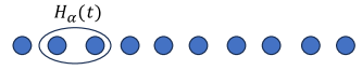
In this work, we will consider a class of lattice models one or more spatial dimensions with “Brownian” time-dependent Hamiltonians. We label one copy of the full Hilbert space . The Hamitonians consist of a sum of local random terms (shown in Fig. 3) which are uncorrelated for different and :
| (13) | |||
| (14) |
We can analyze the dynamics under this setup by formally discretizing the time-evolution in small steps of size , and regularizing the delta function between different times by replacing it with , so that
| (15) |
One simple choice, which we will discuss in Sec. IV, will be to take the matrices themselves to be random. A less random class of models is one where we fix some set of local Hermitian operators , and take the coefficients appearing next to them to be random:
| (16) |
where are random i.i.d. real numbers drawn from a Gaussian distribution, such that
| (17) |
for some arbitrary positive numbers . We can make a variety of choices of , where cases with different symmetries will correspond to different dynamical universality classes [30]. For example, in a spin-1/2 system in spatial dimensions with sites labelled by , we could consider a case where for nearest neighbours . In this case, the time-evolution does not have any symmetry. Another choice is to take . These operators commute with the total charge , so that the time-evolution has a symmetry. 444We can see the symmetries in each case by computing the commutant of the operators (i.e., the algebra of operators that commute with these terms) [39, 30].
The dynamical quantities of interest in this work are the -th Renyi entropies of a subsystem . These can be expressed as transition amplitudes on copies of the system ,
| (18) |
where denotes complex conjugation, and we have introduced a set of states in , associated with an operator acting on , and permutations , which are defined as follows. Let be basis states for one copy of the system. We define
| (19) |
In cases where is the identity operator, it will be convenient to label the corresponding states simply by the permutation, that is,
| (20) |
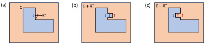
In (18), refers to the identity permutation, and refers to the single-cycle permutation . Further, we can also consider such states with a fixed permutation on the Hilbert space of some subsystem ; in lattice systems with sites labelled by , we have . The final state in the bra in (18) therefore has a domain wall at the boundary between the regions, see Fig. 4. From (18), the evolution of the Renyi entropy of any initial state can be understood in terms of the backward time-evolution of this domain wall final state under . We will make use of this perspective, introduced for instance in [14, 15], in the rest of this work.
Let us label the copies of the system in (18) by , for , corresponding respectively to the forward evolutions by and backward evolutions by . On expanding (15) for a step of size and using the averages in (17), we find
| (21) | |||
By re-exponentiating (21) 555In the rest of this work, we will not explicitly indicate overlines, but in all cases the expression should be interpreted as the average of over the randomness in the time-evolution., we find
| (22) |
In particular, the average over the random allows us to replace the original Lorentzian time-evolution on copies of the system with a Euclidean evolution, with a non-negative “superhamiltonian” . We will first briefly discuss the structure of the zero energy ground states of in Sec. III, and then discuss the structure of its low energy eigenstates in models without conserved quantities in the later sections.
III Late-time saturation value
The superhamiltonian (21) consists of a sum of positive semidefinite operators, so that its eigenvalues are all non-negative. Any zero energy eigenstate must be “frustration-free,” meaning that it is annihilated by each term:
| (23) |
One explicit set of zero energy eigenstates of can be constructed as follows. Let be the set of all operators which commute with all elements of , which is also known as its commutant algebra [39], and characterizes the symmetries of the time-evolution. Let be an orthonormal basis of operators for , i.e., they satisfy . Now for any choice of a sequence and a permutation , let us define a state in :
| (24) |
Here each labels basis states in like in (19), and runs from 1 to , the total Hilbert space dimension, and each goes from 1 to , the dimension of , and labels an element of . Since each commutes with all , the above states are zero energy eigenstates of . Assuming that these states span the ground state subspace of ,666This should be true for generic choices of , and is provable in many cases for [30] but there are exceptions for , e.g., when can be written as quadratic operators in fermions [40, 26]. We also discuss this in Section V. we have the following late-time limit of the Euclidean time-evolution operator:
| (25) |
The above expression assumes that the states in (24) can be treated as approximately orthonormal, which is true for the purpose of the expression (18) when the initial state can access a large effective Hilbert space dimension.777See the example in Appendix A for a more explicit discussion of this point.
Putting this projector into (18), in the case where the initial state is pure, we find
| (26) |
where
| (27) |
is defined as in (19). See Appendix A for details of the derivation. It is natural to think of defined above as an equilibrium density matrix which coarse-grains over all details of other than the information about the conserved charges. We discuss an explicit example in Appendix A for the case where the time-evolution has a symmetry, which makes this interpretation clearer.
It was previously argued in the context of general chaotic quantum many-body systems in [8] that the expression (26) gives the saturation value of the -th Renyi entropy in an equilibrated pure state which macroscopically resembles some equilibrium state . The Brownian models we consider in this work provide one explicit confirmation of this general argument, with a precise form of given by (27). The general properties of the expression (26) are discussed in [8]. In particular, the sum over permutations ensures that the -th Renyi entropy in is equal to that in at late times, as required by the unitarity of the dynamics. In the thermodynamic limit, it is explained in [8] that the dominant permutation in (26) is always either or , leading to the physically expected result in (2).
IV Brownian local GUE model
Let us consider a -dimensional lattice, with a -dimensional Hilbert space at each site. As a first simple model, we take the to be random Hermitian matrices acting on pairs of nearest neighbours on the lattice, and drawn from the GUE ensemble, so that888For a recent discussion of the spectrum of this time-dependent Hamiltonian in the case without spatial locality, see [41].
| (28) |
By similar steps to the discussion around (21), for this model we obtain the following superhamiltonian on (again labelling copies with forward evolution and those with backward evolution , with ):
| (29) |
where is the identity operator in , is the projector onto the maximally entangled state between the copies and at site , , and is the swap operator between copies and at site , which has the action . has a large symmetry group which includes corresponding to permuting the forward and backward copies independently; see [40] for a detailed symmetry analysis of Hamiltonians of this kind.
For , this superhamiltonian has a unique ground state given by , where is two-copy state associated with the identity permuation, see Eq. (20). Moreover, it is easy to check that it is composed of commuting terms, and is therefore exactly solvable, with a gapped spectrum with discretely spaced energy levels. This leads to a simple exponential decay of infinite-temperature autocorrelation functions of any operator , which can be written as
| (30) |
This is consistent with the physical expectation from the lack of any symmetries in the time-evolution.
For general , if we consider the subspace spanned by states of the form for , then keeps this subspace closed. Its zero energy ground states are the product states with the same permutation at each site:
| (31) |
These can be thought of as ferromagnets of degrees of freedom. We hence expect to be gapped, and the low-energy excitations to be domain-walls between the different ferromagnetic ground states. The structure of the low-energy excitations leads to the membrane picture of entanglement.
The saturation value of the -th Renyi entropy in this model obtained from the ground states (31) is the special case of (26) with , where is the total Hilbert space dimension. As discussed in [8], (27) for this case is equal to the average value in random product states [3, 4, 5, 6, 7]. The equilibrium entropy density for each of the Renyi entropies is therefore
| (32) |
IV.1 Second Renyi entropy
Let us now focus on the structure of the superhamiltonian (29) for the case . In this case, we have two degenerate ground states,
| (33) |
where
| (34) |
It will be useful to express in terms of these spin states. Note that and are normalized, but do not form an orthonormal basis as . It will be convenient to work in a bi-orthogonal system and introduce the following two states
| (35) |
which have the property that for . We can then write in the subspace spanned by at each site as follows:
| (36) |
where denotes nearest neighboring sites on a lattice, and for instance denotes . This representation will be useful as the final state in the expression for the second Renyi entropy in (18) is a domain wall state of the form .
While the above representation will be convenient for some of our later analysis, we can also represent in the following orthonormal basis for one site:
| (37) |
Defining the Pauli matrices with respect to these states, where and are the eigenstates of the operator, we obtain the following representation:
| (38) |
In one spatial dimension, lies on a parameter line of the Heisenberg XYZ spin chain in an external magnetic field known as the “Peschel-Emery” line [42, 43]. On this line, the Hamiltonian is known to lie within the Ising ferromagnetic ( symmetry broken) phase, and was previously noted to have two frustration-free product ground states, which are of the form (33). We discuss this mapping in Appendix B.
In the rest of this section, we specialize to one spatial dimension. We will consider higher dimensions in Sec. VI.
 |
 |
 |
IV.1.1 Large limit
Let us first take a large limit by ignoring the term in (36), which is . In one spatial dimension, the left eigenstates of the non-Hermitian Hamiltonian will turn out to be exactly solvable. We assume that the system has sites labelled from to and open boundary conditions (OBC), but we will take for most purposes. Note that the zero energy left-eigenstates of are the same as the zero energy eigenstates of the full Hamiltonian , given by (33). Due to this feature, turns out to be a better first approximation for understanding the structure of the first excited states than the transverse field Ising model obtained by keeping the and terms in (38).
To find the low-energy left-eigenstates, note that has a particularly simple left-action on the domain wall states defined as
| (39) |
given by
| (40) |
where we have implicitly defined at the boundaries. From (40), we can immediately see that the lowest band of left-eigenstates of above the ground state is given by
| (41) |
The spectrum is gapped as we are in the regime .
Let us now apply this structure to understand the evolution of for a half-line region to the left of ,
| (42) |
It is useful to introduce the states , and a “domain wall propagator” (considered for instance in [38])
| (43) |
in terms of which (42) can be written as
| (44) |
Here we have used the fact that the action of does not create additional domain walls, and we can hence insert a resolution of identity restricted to the single domain wall subspace in (42). Then using (41) and working in the limit, we can express (43) as
| (45) |
Let us now take the late-time limit , and consider of in this limit. Then the integral over can be evaluated using the saddle-point approximation. The saddle-point value lies on the imaginary axis, and by deforming the contour to pass through its steepest descent contour we get
| (46) |
where
| (47) |
Now putting (46) into (44), we obtain precisely the membrane formula for the second Renyi entropy in the large limit:999In this discussion, we ignore the difference between and , as in various earlier works including [15, 14].
| (48) |
where in the second step we have used that and , and ignored contributions that are smaller than linear in .
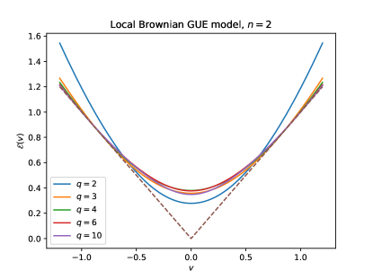
The membrane tension from the dispersion relation (41) is 101010Note that (49) by itself does not satisfy the constraints (4) except in the strict large limit (50). It does satisfy the constraints at finite if we make the replacement , which can be seen as a simple analytical “toy model” for the membrane tension function, see Appendix B.3.
| (49) |
Its strict large limit is
| (50) |
which satisfies the constraints (4) in a somewhat degenerate way. As we will discuss in the following sections, the expressions (44)-(48) will turn out to apply to more general cases than the large limit of the current model. The modified dispersion relations in these cases will lead to other, more general expressions for .
Before discussing these more general cases, let us briefly discuss the form of for a region consisting of one or more intervals in the large limit. Since the “final state” in this case would contain more than one domain wall, we now need to consider “multi-particle” excitations of involving more than one domain wall. For a state with two or more domain walls, we can check from (36) that the left-action of can cause domain walls to annihilate in pairs. It is useful to divide into two parts,
| (51) |
where keeps the number of domain walls fixed, while causes the annihilation of pairs of domain walls. has a block-diagonal structure, while the whole matrix has a lower-triangular structure due to . The energy eigenvalues of are therefore the same as those of . Denoting the multiple domain wall states by , , it is easy to check that the domain walls are “non-interacting” under the action of . Hence, the eigenstates of take a simple free fermion-like Slater determinant form:
| (52) |
with energies given by the sum of the one-particle energies in (41). Hence, the energies of the multiparticle states under are also sums of one-particle energies,111111This is also evident if one performs the basis change of (37) on in (36) and then performs a Jordan-Wigner transformation of (110) – the resulting Hamiltonian is a non-Hermitian non-interacting Hamiltonian. although the eigenstates are more complicated superpositions of (52). As we discuss in more detail in Appendix C, this structure leads to the membrane picture for multiple intervals.
IV.1.2 General structure
The key physical properties of that give rise to the membrane picture in the above discussion are: (i) is gapped, so that has an exponential decay for any initial state, leading to linear growth of ; (ii) the one-particle eigenstates of the are plane waves of domain walls between and ; and (iii) domain walls are non-interacting other than the possibility of pair-wise annihilation. In the next section, we will show that properties (i) and (ii) remain robust for the full Hamiltonian at finite . (ii) is robust up to some local “dressing” of the domain walls. In Sec. IV, we will further show that these properties remain robust for Brownian models with fixed coupling operators. We expect that property (iii) is also robust, but this is harder to show explicitly, and we do not comment further on it until the Discussion section VII.
Due to the robustness of (ii), the formulas (44) and (45) will also apply to the second Renyi entropy in all remaining examples we consider. It is useful at this point to summarize some general consequences of these formulas, which we will use in the later discussion.
For an initial state of the form (5), the evolution of is given by
| (53) |
The saddle-point equations for and in the above integral are:
| (54) |
which imply (6) with the entropy growth rate
| (55) |
where we have used the fact that is an even function. Eq. (47) is equivalent to the statement that is the Legendre transform of ,
| (56) |
which also follows from (7) and was previously noted in [12]. 121212We do not add subscripts in this formula as it will also apply to the higher Renyis.
In particular, for an initial pure product state, the entanglement velocity of the second Renyi entropy is proportional to the gap in the spectrum:
| (57) |
From (55), the constraints (4) or (8) are equivalent to the fact that
| (58) |
Using (54), in terms of the dispersion relation, is given by
| (59) |
Note that the condition (58) does not need to be imposed as an external input. The evolution of the entanglement entropy of for a maximally mixed initial state can be expressed as
| (60) |
By acting with on the left, we get (53) with due to the structure of the low-energy excitations, and by acting on the right, we get a time-independent result due to the fact that is a zero energy eigenstate of . (58) must always be true to ensure consistency between these results.
One interesting aspect of the condition (58) is that it is sensitive to the UV behaviour of the dispersion relation , as it involves an imaginary value of . We will return to the implications of this UV sensitivity in the Discussion section.
IV.1.3 Finite
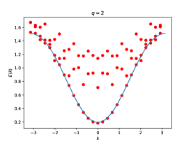
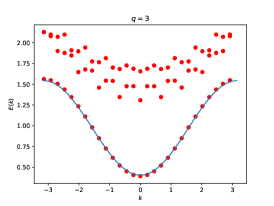
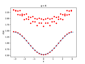
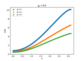
At finite , the term in (36) can send a single domain wall state to a three domain wall state and vice versa, so that the exact low-energy eigenstates are no longer plane waves of single domain walls as in (41), and the exact energies are also modified. Nevertheless, since the ground states of are still ferromagnetic states of the form of (33), we expect the low-energy excitations to be gapped (dressed) domain walls between the two ground states, similar to (41). To numerically determine the momentum-resolved dispersion of the low-energy eigenstates, we study with symmetry-twisted (antiperiodic) boundary conditions, as discussed in Appendix B.131313We thank Tibor Rakovszky for useful discussions on this.,141414In summary, the momentum resolution cannot be obtained directly with a finite-size OBC Hamiltonian due to lack of translation-invariance. On the other hand, periodic boundary conditions (PBC) does not allow for an odd number of domain walls. By inserting a symmetry twist at the boundary, one domain wall gets pinned at the boundary while the other can disperse, and we can obtained the momentum-resolved dispersion of a single domain wall. This is expected to match the low-energy spectrum to match that of the OBC Hamiltonian for large system sizes.
The low-lying spectrum as a function of is shown in Fig. 5 for . In all cases, we find that is gapped, consistent with expectations in the ferromagnetic phase. The gap leads to a linear growth of entanglement for a product state, according to (57). To verify the robustness of the membrane picture, we need to further address the following questions:
-
1.
For , we find a single-particle band in the spectrum well-separated from the multi-particle continuum for all . It is natural to expect that the eigenstates in this band have a quasiparticle structure [35]. Can these quasiparticle states be understood as locally dressed versions of the domain wall states in (41) in a precise sense?
-
2.
For , the gap between the single-particle states and the multi-particle continuum vanishes beyond some value of . Are there still well-defined quasiparticle states within the continuum at large ?
Both questions can be simultaneously addressed using a technique for obtaining low-energy dispersion relations along the lines of [35, 36, 37]. These references introduced a general variational ansatz for low-energy excitations of gapped spin chain systems, starting from the assumption that the ground state is well-approximated by a matrix product state. In the case of the Hamiltonian , since we know that the exact zero energy eigenstates are the product states and , we can use a particularly simple version of the general ansatz:
| (61) |
where is an arbitrary state in the subspace spanned by on sites, which has total Hilbert space dimension . 151515The actual dimension of the subspace spanned by the states in (61) is slightly smaller than due to the redundancy between certain choices of in the thermodynamic limit. For example, for , there is only one linearly independent choice , and for , we can consider an arbitrary superposition of the form .

We increase the value of starting from , and minimize the expectation value over all choices of for a given . We explain details of the variational optimization in Appendix D. As discussed in [35, 36, 37], rapid convergence of the dispersion relation on increasing indicates that the eigenstates of are well-approximated by (61) for , and this interpretation also holds when the dispersion relation lies within a multi-particle continuum. The results are shown in Fig. 6, where we find rapid convergence of the dispersion relation with for all values of for both and . We also compare the variational dispersion relations to the energies obtained from exact diagonalization in Fig. 5, finding good agreement in cases where the latter show a well-defined single-particle band. The expectation value with already gives a good approximation for the numerically observed dispersion relation, see Appendix B.3 for details.
These results confirm that the low-energy eigenstates relevant for the evolution of have the structure of localized domain wall-like states at finite , including in the case at all . Putting this structure (61) of the eigenstates into (42), we have: 161616Note in particular that in the case, even though the energies of the multi-particle continuum are comparable to those of the single-particle band, the final state has significant overlap only with the eigenstates of the single particle band, so that the approximation in (62) is valid.
| (62) |
Since is some superposition of configurations of and spins, for of , the factor in the last line of (62) contains a term proportional to , as well as terms proportional to for all odd , for some . Since is , in the scaling limit of late time and large system size, the differences between these terms can be ignored, and they can be combined into for some number . Similarly, the factor in the first line of (62) can be replaced with in this limit. Hence, the analysis of (43)-(48) also applies to this case, with the change that should be used to denote the numerically obtained exact dispersion relation at finite from Fig. 5, instead of the large- dispersion relation of (41).
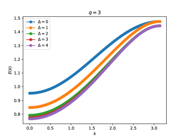
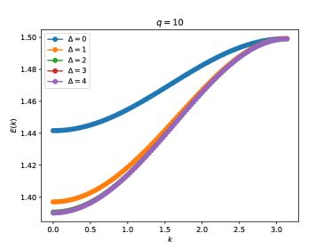
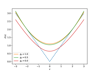
We determine by fitting to the general form
| (63) |
for some finite , and then numerically solving the equation for in (47). This procedure gives us the membrane tensions in Fig. 7. Let us make a few observations about these results:
- 1.
-
2.
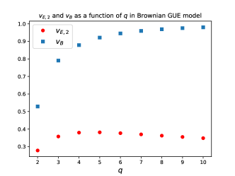
The entanglement velocity from (57) is non-monotonic as a function of , increasing up to and then decreasing. The eventual decreasing behaviour is consistent with the large limit (50). Note, however, that the quantity , which determines the coefficient of the linear growth of for a product state with time, increases monotonically with .
-
3.
The butterfly velocity from (59) monotonically increases with .
We note one subtlety of the above discussion. For any choice of at which we choose to truncate the approximation (61), there will be small corrections in the exact eigenstate proportional to for . In principle, there could be initial states with entanglement structures that would lead to a non-trivial competition in (42) between the suppression of such components in the eigenstate, and an enhancement of the corresponding overlap factor . We argue in Appendix E using a somewhat different approach that such corrections are not important. This argument makes use of the convexity of the numerically obtained membrane tensions in Fig. 7, together with the structure of the interaction picture diagrams we get from treating as a perturbation.
IV.1.4 Comparison to Haar random unitary circuits
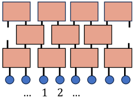
It is instructive to rephrase the evolution of the second Renyi entropy in the brickwork Haar random circuits of [14, 15] in the above language of low-energy modes of a one-dimensional quantum Hamiltonian, as an alternative to the standard discussion in terms of a mapping to a two-dimensional classical statistical mechanics problem. In these models, we apply two-site random unitaries drawn with the Haar measure in the pattern shown in Fig. 8. The average for an even time can be written in the notation of the previous subsections as
| (64) |
Note that is not Hermitian. We can see that , are left eigenstates of with eigenvalue 1, and that in (41) (with the sum restricted to odd , hence the momentum restricted to ) is an exact left eigenstate of for any value of , with eigenvalue , where
| (65) |
Applying the relation (47) for this dispersion relation gives a simple derivation of the membrane tension for this case, previously found in [12]. Unlike the membrane tensions in the Brownian models in the rest of this work, in this model diverges for and is not well-defined for , indicating the sharp light-cone in Haar-random circuits.
One difference between the four-copy evolution by (64) for the Haar random circuit and the evolution by for the local GUE model is the fact that a single domain wall can split into multiple domain walls under the latter but not the former. From the discussion of the previous subsection and Appendix E, we learn that this splitting of the domain walls does not have a qualitative effect on the membrane picture for the second Renyi entropy, and only serves to renormalize the membrane tension. In Appendix F, we give an example of a physical quantity related to operator growth which does show a qualitative difference between Haar random circuits and the GUE model due to this domain wall splitting.
IV.2 Higher Renyi entropies
Let us now discuss the structure of the superhamiltonian of (29) in the more general case where . Recall from the discussion around (31) that the relevant Hilbert space at each site has dimension , and is spanned by the states . The ground states are given by ferromagnetic states of the form (31). For studying the excitations, it is convenient to introduce the notion of the Cayley distance between two permutations , which is the minimum number of transpositions (swaps) needed to go from to . For any such that , we have
| (66) |
Comparing to (36), we see that the action of on states constructed only from any such pair is identical to the action of on . Indeed, this reduction is needed to ensure that we get consistent results on computing the quantity using a general . Hence, the subspaces spanned by configurations of such pairs are closed under the action of . Following the discussion in the case in Sec. IV.1, we have eigenstates of approximately given by plane waves of domain walls between each and , with the same dispersion relations as those found in Fig. 5. However, the action of on permutations , with is not as simple as (66), and this complicates their analysis, as we discuss below.
Recall from (18) that the final state that appears in the expression for is , where . Since for , it turns out that the subspace spanned by configurations of and is not closed, and there is no exact eigenstate of consisting only of and .
To analyze this case, let us start with the following variational ansatz for the excitations of in the sector with towards the left boundary and states towards the right boundary171717We look for eigenstates which asymptotically have this form so that they have non-negligible overlap with the final state in the expression for .
| (67) |
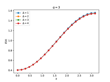
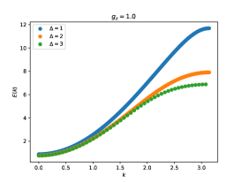
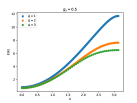
where is some state in the -dimensional Hilbert space consisting of all possible permutation states on sites. Like in Sec. IV, we minimize the expectation value over all possible choices of for increasing values of , and check whether the resulting estimate for the dispersion relation converges with . We show the results of this procedure for with from 0 to 4 in Fig. 9. We find rapid convergence for for all values of . Like in the case of , the convergence with is increasingly fast for larger . We therefore learn that the lowest energy excitations in the relevant sector are well-approximated by (67) for .
Let us now discuss the consequences of (67) for the time-evolution of the -th Renyi entropy. For general , it is useful to define the domain wall propagator (similar to (43)) as
| (68) |
where is defined such that
| (69) |
We assume that the -th Renyi entropy in the scaling limit is well-approximated by
| (70) |
which can be justified by arguments analogous to those below (62). Putting (67) and the corresponding dispersion relation into (70), for an initial state with entropy density for the -th Renyi entropy, analogous to (53), we find
| (71) |
The saddle-point equations for and are
| (72) |
which lead to the following growth rate for the -th Renyi entropy:
| (73) |
An example of from (73) for and (with ) is shown in Fig. 10. Again, we find this function by fitting to the form (63). The figure also shows for the second Renyi entropy from the dispersion relation for the same value of . We see that while obeys the condition (8) needed to ensure that of the equilibrium state should not grow, the curve for appears to not obey this condition. This implies it gives the unphysical prediction that the of the equilibrium state increases rapidly. By similar reasoning to the discussion around (60), we know that this prediction cannot be correct.
In the above discussion, we made the approximation in the expression for , for from (67). The above unphysical conclusion must be prevented by contributions to from a different set of energy eigenstates which we have not taken into account. We now conjecture a possible structure of these other eigenstates which can give a simple resolution of the above issue.
Recall from the discussion around (66) at the beginning of this section that domain walls between permutations of Cayley distance 1 can still be thought of as elementary excitations of for , although these eigenstates would have a very small overlap with the final state . A natural guess for a “multi-particle” version of these elementary excitations, which would have significant overlap with the final state, would be of the approximate form
| (74) |
where we have defined
| (75) |
Since (74)has the structure of a state of free particles, we would expect the energies of the states (74) to be , where is the dispersion relation found numerically for the second Renyi entropy in Sec. IV.1.3. We can check numerically that obtained from the variational calculation in Fig. 9 is smaller than the energies of these hypothetical states with free single-transposition domain walls:
| (76) |
This can be interpreted as the result of an attractive interaction between the single-transposition domain walls, which causes the lowest-energy eigenstates in the relevant sector to be “bound states” of elementary domain walls of the form (67). A similar attractive attraction was also argued for using different techniques in random unitary circuits [16].
Even though the lowest excitations are “bound states,” states of the form (74) may still be present as higher excited states in the spectrum of . We will assume this in the rest of the discussion. 181818It would be challenging to numerically check that these states are present in the spectrum by exact diagonalization due to the large on-site Hilbert space dimension of the superhamiltonian, which allows us to access only small system sizes. However, we comment on other methods that can be used to check this in the Discussion. Such states would give a contribution to the domain wall propagator , which would be added to contribution from the states (67).
By putting this into the expression for , we would get a sum of two terms:
| (77) |
From the competition between the two terms, the true growth rate for the third Renyi entropy at late times is given by
| (78) |
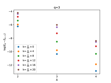
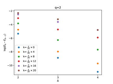
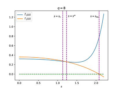
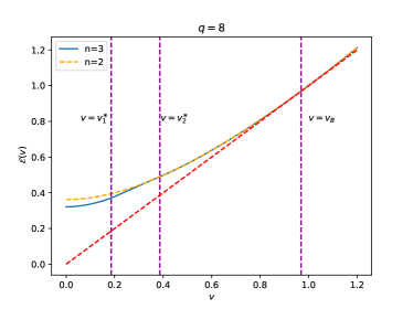
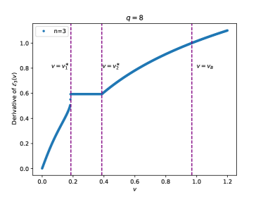
At the critical value where and cross (see Fig. 10), (78) implies a first-order phase transition in . For , , so that in particular the constraint (8) is satisfied. We show the particular case , but we find that the curves cross at all values of that we checked, from to . The ratio appears to increase monotonically with .
Using the general formula (56), we can find the membrane tension as the Legendre transform of . Assuming (78), there are three possible sources of the maximum value in the Legendre transform: it could come either from the region , where , or from the endpoint at , or from the region . We find three distinct regimes for the behaviour of depending on which of these options dominates:
| (79) |
Here is the Legendre transform of restricted to the regime where it is convex 191919Note that the Legendre transform of the full function is not well-defined as it is not convex., and is the value of at which the second derivative of changes from negative to positive. is the membrane tension for the second Renyi entropy found previously. The two critical velocities are
| (80) |
In Fig. 11, we show the membrane tension of (79) obtained from and of Fig. 10, and its first derivative. The membrane tension has a first-order phase transition at , and a second-order phase transition at .
We now make a brief technical note on the difference of the analysis we used above from the case. In this discussion of this section, we did not directly use the domain wall propagator (68) to derive the membrane tension, but instead found it indirectly as the Legendre transform of . The form of the dispersion relation is such that the domain wall propagator from the states (67),
| (81) |
can be used to obtain the membrane tension only up to by similar steps to (47). For , the propagator has an oscillating behaviour with time due to a change in the structure of the solutions to the saddle-point equation . The propagator in this regime does not contribute to the evolution of the entropy in the combined saddle-point analysis in the integral over and for . From the saddle-point equations (71), we get a well-defined result for for any . The Legendre transform of by itself is again not well-defined beyond , but the Legendre transform of the negative of (78) is well-defined, as discussed above, and this should be seen as the definition of the membrane tension for this case. 202020We thank Raghu Mahajan and Douglas Stanford for helpful discussions on the saddle point analysis.
In [16], the membrane tension for the third Renyi entropy was studied for random unitary circuits. The calculations in that context, which were done in expansions for large and large , also gave indication of a phase transition in . The physical mechanism suggested for the “unbinding” phase transition there appears similar to the one discussed here. From the calculations in the present model at finite and general , we see that there are two phase transitions in . Unlike in the large random circuit calculation of [16], where the critical velocity appeared to be , we find that both critical velocities are smaller than at finite .
V Brownian models with fixed coupling operators
|
Let us now consider the family of models in (16), where the coupling coefficients are random and uncorrelated, but the operators are fixed and act on a system with a -dimensional on-site Hilbert space. This is a less random and hence more realistic example of a chaotic system than the one considered in Sec. IV.
The superhamiltonian (21) for this case still has the property that any of its terms that has support on sites annihilates configurations of the form on those sites for any . This implies that the states (31) are still ground states in this case. In cases where the time-evolution has no symmetries, we expect that these are generically a complete basis for the ground state subspace, so that the saturation value of is given by the Page value [44], and .
Unlike in the GUE case, the action of a general can now take a general initial state with different permutation states at different sites into the subspace orthogonal to all the permutation states, hence the effective Hilbert space on each site is now -dimensional, rather than dimensional in the GUE case. However, since the ground states are still of the ferromagnetic form of (31), it is natural to once again conjecture that the low-energy excitations are well-approximated by the structure in (11) for , with the state now living in the full -dimensional Hilbert space.
Numerically, it is feasible to test the above conjecture using the variational technique of Appendix D up to for and , where the maximum Hilbert space dimension of the effective Hamiltonian for the variational problem (see Appendix D) is . For concreteness, let us take the set of coupling operators to be the following spin- operators in a one-dimensional system of sites:
| (82) |
Taking the in the variance of the couplings (17) to be some positive numbers respectively. In the discussion below, we will fix , and consider a variety of different values of . We expect this time-evolution to be chaotic for generic values of , except at the point , where the time-dependent Hamiltonian is only a linear superposition of and operators and hence has a quadratic (non-interacting) Majorana fermion representation using the Jordan-Wigner transformation.
We show the results of the variational method for this family of models in Fig. 12, which confirms the expectation that the eigenstates have the structure (11) for generic . The dispersion relation in the cases and converges rapidly. For , corresponding to the free fermion case, the dispersion relation shows slower convergence.
The Brownian free Majorana fermion evolution corresponding to was previously studied in [26], where it was found that can be mapped to the ferromagnetic Heisenberg model. The ground state subspace for this case is much larger than the one spanned by (33), and it has gapless low-energy excitations which lead to a growth of proportional to rather than . Hence, the variational ansatz (11) is likely to not be a good approximation to the true low energy eigenstates for , consistent with our observations.
The closing of the gap of (or equivalently vanishing of the entanglement velocity ) can be seen as a precise information-theoretic signature of a transition from chaotic to free-fermion integrable behaviour in this family of models. Any non-zero causes the model to lose its free fermion character and recover the general features of chaotic many-body systems, hence opening up a gap in the thermodynamic limit. At finite system size, we expect a crossover from chaotic to integrable behaviour at small , similar to the discussion in [26].
While we do not have an independent check of the dispersion relations from exact diagonalization of in the above family of models (due to the large on-site Hilbert space dimension ), we have performed the following two consistency checks, which verify that the dispersion relation is close to convergence for and far from convergence for :
-
1.
We directly evaluated the amplitude using the TEBD method for imaginary time evolution [45] for an initial pure product state . For generic values of , we find that this quantity has an exponential decay regime for a large range of times, corresponding to linear growth of the entropy. This gives an independent calculation of the entanglement velocity defined in the first equation of (57), which can be compared to the one found from the gap of the dispersion relation. For , we find good agreement up to about of the values, which are expected from the level of precision on both sides of the calculation. For , we do not see a linear growth regime from TEBD.
- 2.
VI Membrane picture in general spatial dimensions
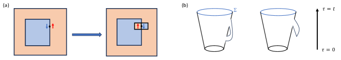
Let us briefly discuss how the above picture generalizes to higher spatial dimensions . It is useful to return to the simplest case of the second Renyi entropy in the Brownian GUE model, where the superhamiltonian in arbitrary dimensions is given by (36) or (38). To find the second Renyi entropy of a region with boundary , the final state in (18) is a domain wall between and along , as shown in Fig. 14(a), which we call . As a first approximation in the large limit, let us again ignore the term of (36). Even with this simplification, it is not straightforward in to diagonalize in the subspace relevant for the evolution of for . However, we can obtain an expression for the evolution of for an infinitesimal time-step of length by noting that
| (83) |
where correspond to inward or outward deformations of by a single lattice site in the direction normal to the surface at .212121We assume that the shape of the initial surface is such that it does not pinch off and split into two domain walls in time . See Fig. 14 for an illustration in . Hence, close to a small segment of the domain wall, the dynamics in higher dimensions resemble the one-dimensional dynamics in (40) in the direction normal to the surface.
Now by linearizing the evolution of for a short time , we find
| (84) |
By taking continuum approximations for the differences and sums in the above expression, we obtain
| (85) |
For the second Renyi entropy, on ignoring a second derivative term which is negligible in the scaling limit of large system size and late time, (85) is equivalent to
| (86) |
where
| (87) |
As discussed in [12], a differential equation of the form (86) is equivalent to the membrane formula in arbitrary dimensions with given by (56), which for this case is
| (88) |
independent of the spatial dimension . In particular, the above series of steps are valid in the case , where on comparing to (49), we see that we have obtained the membrane tension we would get from taking first the large and then the small limit in . Recall that in order to satisfy the constraints (4), the higher order terms in both and were important. In order to go beyond the quadratic approximation in , we would need to find an alternative to taking the continuum limit in (84). The higher order corrections in would come from incorporating corrections from the term in the last line of (36), which causes domain walls to split as shown in Fig. 15 (a), and gives rise to spacetime diagrams like those in Fig. 15 (b) which should renormalize the membrane tension. These are analogous to the diagrams for discussed in Appendix E.1, which provided an alternative way of understanding corrections to the dispersion relation and membrane tension away from the large . It would be interesting to quantitatively incorporate the effects of such diagrams and see whether they lead to a dimension-dependent membrane tension, as observed in holographic CFTs [17].
Finally, we note that the superhamiltonian for the GUE model on any lattice in one or higher dimensions is the Peschel-Emery Hamiltonian of Eq. (38) on that lattice. For large , the low-energy physics of this Hamiltonian is expected to resemble that of the Transverse-Field Ising Model (TFIM) in the presence of a “weak” field of , which is the Hamiltonian obtained by ignoring the term in Eq. (38). Indeed, as discussed in Sec. IV.1, many of the properties of in one dimension are similar to those of the one dimensional TFIM, e.g., the symmetry broken degenerate ground states and the structure of the low-energy domain wall excitations. It is natural to expect similar connections in higher dimensions too at least for large , i.e., the entanglement membrane picture in higher dimensions should be related to the low-energy physics of higher dimensional transverse field Ising models in a weak field. It would be interesting to explore this connection in future work.
VII Conclusions and Discussion
In this work, we have identified the microscopic mechanism which is responsible for the emergence of the membrane picture of entanglement dynamics in “Brownian” time-evolutions of the form (14). The Lorentzian time-evolution of the Renyi entropies in such models can be mapped to a Euclidean evolution by a “superhamiltonian” living on multiple copies of the system. We first considered a maximally random Brownian GUE model in spatial dimension, where we showed that the membrane picture for the second Renyi entropy emerges from the fact that the low-energy excited states of this superhamiltonian take the form of plane waves of certain locally dressed domain walls between symmetry broken ground states. We confirmed this structure using analytical perturbative techniques and exact diagonalization, as well as variational numerical techniques for probing the low-energy eigenstates.
We further used the variational techniques to study the third Renyi entropy, and argued that in this case, the membrane tension exhibits a first order as well as a second order phase transition as a function of velocity. Finally, we provided evidence that the same structure of low-energy modes appears in more generic examples of Brownian models, independent of details of the interactions. The membrane tensions in all cases are determined by the dispersion relations of the low-energy modes, and we showed that they satisfy the expected physical constraints. Collectively, these examples provide an understanding of how universality emerges in the late-time dynamics of entanglement entropies in this class of quantum many-body systems.
While the above derivation of the membrane formula from the microscopic dynamics is specific to this particular class of models, it would be interesting to use these lessons to build an effective theory for more general chaotic systems, including fixed Hamiltonians without any randomness. Some motivation that the structure found here should extend to more general systems comes from considering the superhamiltonians (living on two copies of the system) in -conserving versions of these models, previously studied in [30, 31]. These papers found that the diffusive behaviour of the two-point functions of the charge density comes from certain gapless low-energy eigenstates of the superhamiltonian. These gapless excitations can be seen as a precise realization of the hydrodynamic modes which are expected to govern diffusive behaviour of two-point functions much more generally. Alternative approaches which start from the assumption that such gapless modes exist have previously been used to construct effective field theories of hydrodynamics [46, 47].
It is then natural to ask whether one can formulate an effective field theory for entanglement dynamics based on the set of low-lying modes living on four or more copies that we found in this work. Note that any such effective field theory would need to contain several new elements relative to those developed in earlier works [47, 46]. The modes leading to the membrane picture differ from hydrodynamic modes in that they are not associated with any symmetry of the time-evolution, and are gapped. 222222The fact that the modes are gapped is needed to ensure exponential decay of , or equivalently linear growth of the entropies. Moreover, even above the gap, the dispersion relation at values of the momentum is physically relevant. In particular, since , a small expansion of the dispersion relation will not satisfy the condition (58); this UV sensitivity suggests that the conventional approach of derivative expansions might not be the right way to formulate the relevant EFT.
In holographic theories, the modes that lead to diffusion in the boundary conformal field theory correspond to quasinormal modes in the bulk gravity dual [48]. Based on the results of this work, it is natural to ask what the analog of these quasinormal modes is for observables like the -th Renyi entropy and the von Neumann entropy. It would be interesting to identify such modes in the replicated geometries for the -th Renyi entropy in the prescription of [49, 50], as well as their analytic continuation to .
In the context of higher Renyi entropies, a better understanding the phase transition that we found in is highly desirable. At a technical level, it would be good use the methods of [37] for probing multi-quasiparticle excitations to check the existence of the excited states (74), which is assumed in obtaining our expression (78). At a conceptual level, there are interesting questions about what this phase transition means information-theoretically. In particular, beyond , we find that becomes equal to , which in particular implies that defined through (4) is the same for and . Is there a simple physical reason why the butterfly velocity according to this definition should be the same for all the Renyi entropies? It would also be good to collect more data on such phase transitions in more general Brownian models and for , which would require technical improvements to the variational methods used in this work, for instance by combining them with a matrix product state (MPS) ansatz (see [51] for a review). The physical existence of these transitions in generic non-Brownian models or time-independent systems should also be verified more carefully, for example using direct computations of the entropies.
The methods developed in [37] and their extensions could also be useful for a number of related questions. Recall that in the large limit, to show the membrane picture for multiple intervals even for the second Renyi entropy, we used the fact that multiple domain walls were essentially non-interacting in this limit. For the membrane picture for multiple intervals to be robust at finite and in more general cases, the quasiparticles consisting of dressed domain walls should be weakly interacting, which can be checked using such numerical methods. Higher dimensional generalizations of these methods could also be useful in understanding the physical picture for entanglement growth in higher dimensional systems, which were discussed in Section VI.
It is important to understand how the physical picture of this work is modified in cases where the system has conservation laws. The simplest such case one can consider is to take Brownian models like the ones studied in this work with an additional conservation law. Renyi entropies in systems with conservation are said to show a growth [52, 53, 54], however a universal underlying mechanism and the extent to which these results hold [55, 56] is still not clear. In this case, there is an interesting and rather intricate coupling between the domain wall degrees of freedom discussed in this work, and the hydrodynamic degrees of freedom associated with the conserved charge density. We plan to report these on results in upcoming work.
This interplay between the entanglement domain walls and hydrodynamic modes can also be explored for a variety of other symmetries, such as dipole or multipole conservation [57, 58, 59], or other unconventional symmetries such as quantum many-body scars [60, 61] and Hilbert space fragmentation [39, 62], hydrodynamic modes of which were derived using the superhamiltonian in [31, 30].
The superhamiltonians found in this work govern the evolution not only of the Renyi entropies, but also of other interesting dynamical quantities that probe chaos and thermalization. In particular, the out-of-time-ordered correlator (OTOC) can also be written as a transition amplitude under :
| (89) |
where we use the notation of Sec. II, and and are the spatial locations of the two operators. By putting the eigenstates of that we found in (11) into this expression, we obtain the following expression for the OTOC, previously noted in [38, 63] (assuming that , and after an average over unitary rotations of the operators , which allows us to write the boundary conditions for this quantity in terms of [38]):
| (90) |
Using the constraints , we see that if , then is included in the sum over , so that . If , then the OTOC starts to decay, and is dominated by the endpoint contribution from in (90) due to the convexity of . By expanding close to and using (4), we find the diffusive broadening of the operator front first noted in [15, 14]:
| (91) |
A particular case where this structure should applyis in the Brownian SYK model [20, 21]. In this model, there is an alternative effective description in a certain large limit in terms of collective degrees of freedom known as “scramblons.” The diffusive broadening (91) is very non-trivial to derive from the Feynman diagrams of the scramblon field theory [64]. It would be interesting to understand how the effective modes found in the present work emerge from the scramblons in the appropriate late-time limit.
Acknowledgements
We thank Henry Lin and Tibor Rakovszky for early collaboration on this work. We are grateful to Hosho Katsura, Shota Komatsu, Marco Lastres, Hong Liu, Frank Pollmann, Xiaoliang Qi, Raghu Mahajan, Mark Mezei, Lesik Motrunich, and Douglas Stanford for useful discussions, Raghu Mahajan for helpful comments on the draft, and Frank Pollmann for helpful numerical suggestions. SM thanks Lesik Motrunich for collaboration on a previous work [30], and Marco Lastres and Frank Pollmann for collaboration on an upcoming work. SV is supported by Google. We acknowledge the hospitality of the Yukawa Institute of Theoretical Physics (YITP), Kyoto during the workshop “Quantum Information, Quantum Matter and Quantum Gravity” (YITP-T-23-01), where this work was initiated.
References
- Banks et al. [1998] T. Banks, M. R. Douglas, G. T. Horowitz, and E. Martinec, AdS Dynamics from Conformal Field Theory, arXiv e-prints (1998), arXiv:hep-th/9808016 [hep-th] .
- Balasubramanian et al. [1999] V. Balasubramanian, P. Kraus, A. Lawrence, and S. P. Trivedi, Holographic probes of anti-de Sitter spacetimes, Phys. Rev. D 59, 104021 (1999), arXiv:hep-th/9808017 [hep-th] .
- Page [1993] D. N. Page, Average entropy of a subsystem, Phys. Rev. Lett. 71, 1291 (1993), arXiv:gr-qc/9305007 [gr-qc] .
- Lubkin [1978] E. Lubkin, Entropy of an n-system from its correlation with a k-reservoir, Journal of Mathematical Physics 19, 1028 (1978).
- Lloyd and Pagels [1988] S. Lloyd and H. Pagels, Complexity as thermodynamic depth, Annals of Physics 188, 186 (1988).
- Nadal et al. [2011] C. Nadal, S. N. Majumdar, and M. Vergassola, Statistical Distribution of Quantum Entanglement for a Random Bipartite State, Journal of Statistical Physics 142, 403 (2011), arXiv:1006.4091 [cond-mat.stat-mech] .
- Leutheusser and Van Raamsdonk [2017] S. Leutheusser and M. Van Raamsdonk, Tensor network models of unitary black hole evaporation, Journal of High Energy Physics 2017, 141 (2017), arXiv:1611.08613 [hep-th] .
- Liu and Vardhan [2021] H. Liu and S. Vardhan, Entanglement entropies of equilibrated pure states in quantum many-body systems and gravity, PRX Quantum 2, 010344 (2021).
- Kim and Huse [2013] H. Kim and D. A. Huse, Ballistic Spreading of Entanglement in a Diffusive Nonintegrable System, Phys. Rev. Lett. 111, 127205 (2013), arXiv:1306.4306 [quant-ph] .
- Liu and Suh [2014] H. Liu and S. J. Suh, Entanglement Tsunami: Universal Scaling in Holographic Thermalization, Phys. Rev. Lett. 112, 011601 (2014), arXiv:1305.7244 [hep-th] .
- Hartman and Maldacena [2013] T. Hartman and J. Maldacena, Time evolution of entanglement entropy from black hole interiors, Journal of High Energy Physics 2013, 14 (2013), arXiv:1303.1080 [hep-th] .
- Jonay et al. [2018] C. Jonay, D. A. Huse, and A. Nahum, Coarse-grained dynamics of operator and state entanglement, arXiv e-prints (2018), arXiv:1803.00089 [cond-mat.stat-mech] .
- Nahum et al. [2017] A. Nahum, J. Ruhman, S. Vijay, and J. Haah, Quantum Entanglement Growth under Random Unitary Dynamics, Physical Review X 7, 031016 (2017), arXiv:1608.06950 [cond-mat.stat-mech] .
- Nahum et al. [2018] A. Nahum, S. Vijay, and J. Haah, Operator Spreading in Random Unitary Circuits, Physical Review X 8, 021014 (2018), arXiv:1705.08975 [cond-mat.str-el] .
- von Keyserlingk et al. [2018] C. W. von Keyserlingk, T. Rakovszky, F. Pollmann, and S. L. Sondhi, Operator Hydrodynamics, OTOCs, and Entanglement Growth in Systems without Conservation Laws, Physical Review X 8, 021013 (2018), arXiv:1705.08910 [cond-mat.str-el] .
- Zhou and Nahum [2019] T. Zhou and A. Nahum, Emergent statistical mechanics of entanglement in random unitary circuits, Phys. Rev. B 99, 174205 (2019), arXiv:1804.09737 [cond-mat.stat-mech] .
- Mezei [2018] M. Mezei, Membrane theory of entanglement dynamics from holography, Phys. Rev. D 98, 106025 (2018), arXiv:1803.10244 [hep-th] .
- Lashkari et al. [2013] N. Lashkari, D. Stanford, M. Hastings, T. Osborne, and P. Hayden, Towards the fast scrambling conjecture, Journal of High Energy Physics 2013, 22 (2013), arXiv:1111.6580 [hep-th] .
- Xu and Swingle [2019] S. Xu and B. Swingle, Locality, Quantum Fluctuations, and Scrambling, Physical Review X 9, 031048 (2019), arXiv:1805.05376 [cond-mat.str-el] .
- Saad et al. [2018] P. Saad, S. H. Shenker, and D. Stanford, A semiclassical ramp in SYK and in gravity, arXiv e-prints (2018), arXiv:1806.06840 [hep-th] .
- Sünderhauf et al. [2019] C. Sünderhauf, L. Piroli, X.-L. Qi, N. Schuch, and J. I. Cirac, Quantum chaos in the Brownian SYK model with large finite N : OTOCs and tripartite information, Journal of High Energy Physics 2019, 38 (2019).
- Bauer et al. [2017] M. Bauer, D. Bernard, and T. Jin, Stochastic dissipative quantum spin chains (I) : Quantum fluctuating discrete hydrodynamics, SciPost Phys. 3, 033 (2017).
- Bauer et al. [2019] M. Bauer, D. Bernard, and T. Jin, Equilibrium fluctuations in maximally noisy extended quantum systems, SciPost Phys. 6, 045 (2019).
- Bernard and Piroli [2021] D. Bernard and L. Piroli, Entanglement distribution in the quantum symmetric simple exclusion process, Phys. Rev. E 104, 014146 (2021).
- Bernard et al. [2022] D. Bernard, F. H. L. Essler, L. Hruza, and M. Medenjak, Dynamics of fluctuations in quantum simple exclusion processes, SciPost Phys. 12, 042 (2022).
- Swann et al. [2023] T. Swann, D. Bernard, and A. Nahum, Spacetime picture for entanglement generation in noisy fermion chains, arXiv e-prints (2023), arXiv:2302.12212 [cond-mat.stat-mech] .
- Zhou and Chen [2019] T. Zhou and X. Chen, Operator dynamics in a Brownian quantum circuit, Phys. Rev. E 99, 052212 (2019).
- Jian and Swingle [2021] S.-K. Jian and B. Swingle, Note on entropy dynamics in the Brownian SYK model, Journal of High Energy Physics 2021, 42 (2021).
- Jian et al. [2022] S.-K. Jian, G. Bentsen, and B. Swingle, Linear Growth of Circuit Complexity from Brownian Dynamics, arXiv e-prints (2022), arXiv:2206.14205 [quant-ph] .
- Moudgalya and Motrunich [2023] S. Moudgalya and O. I. Motrunich, Symmetries as Ground States of Local Superoperators, arXiv e-prints (2023), arXiv:2309.15167 [cond-mat.stat-mech] .
- Ogunnaike et al. [2023] O. Ogunnaike, J. Feldmeier, and J. Y. Lee, Unifying Emergent Hydrodynamics and Lindbladian Low-Energy Spectra across Symmetries, Constraints, and Long-Range Interactions, Phys. Rev. Lett. 131, 220403 (2023).
- Calabrese and Cardy [2007] P. Calabrese and J. Cardy, Entanglement and correlation functions following a local quench: a conformal field theory approach, Journal of Statistical Mechanics: Theory and Experiment 2007, 10004 (2007), arXiv:0708.3750 [cond-mat.stat-mech] .
- Leichenauer and Moosa [2015] S. Leichenauer and M. Moosa, Entanglement tsunami in (1 +1 )-dimensions, Phys. Rev. D 92, 126004 (2015), arXiv:1505.04225 [hep-th] .
- Casini et al. [2016] H. Casini, H. Liu, and M. Mezei, Spread of entanglement and causality, Journal of High Energy Physics 2016, 77 (2016), arXiv:1509.05044 [hep-th] .
- Haegeman et al. [2013] J. Haegeman, S. Michalakis, B. Nachtergaele, T. J. Osborne, N. Schuch, and F. Verstraete, Elementary Excitations in Gapped Quantum Spin Systems, Phys. Rev. Lett. 111, 080401 (2013), arXiv:1305.2176 [quant-ph] .
- Haegeman et al. [2012] J. Haegeman, B. Pirvu, D. J. Weir, J. I. Cirac, T. J. Osborne, H. Verschelde, and F. Verstraete, Variational matrix product ansatz for dispersion relations, Phys. Rev. B 85, 100408 (2012), arXiv:1103.2286 [quant-ph] .
- Vanderstraeten et al. [2015] L. Vanderstraeten, F. Verstraete, and J. Haegeman, Scattering particles in quantum spin chains, Phys. Rev. B 92, 125136 (2015), arXiv:1506.01008 [cond-mat.str-el] .
- Zhou and Nahum [2020] T. Zhou and A. Nahum, Entanglement Membrane in Chaotic Many-Body Systems, Physical Review X 10, 031066 (2020), arXiv:1912.12311 [cond-mat.str-el] .
- Moudgalya and Motrunich [2023] S. Moudgalya and O. I. Motrunich, From symmetries to commutant algebras in standard Hamiltonians, Annals of Physics 455, 169384 (2023).
- Bao et al. [2021] Y. Bao, S. Choi, and E. Altman, Symmetry enriched phases of quantum circuits, Annals of Physics 435, 168618 (2021), special issue on Philip W. Anderson.
- Tang [2024] H. Tang, Brownian Gaussian Unitary Ensemble: non-equilibrium dynamics, efficient -design and application in classical shadow tomography, arXiv e-prints (2024), arXiv:2406.11320 [hep-th] .
- Peschel and Emery [1981] I. Peschel and V. J. Emery, Calculation of spin correlations in two-dimensional Ising systems from one-dimensional kinetic models, Zeitschrift für Physik B Condensed Matter 43, 241 (1981).
- Katsura et al. [2015] H. Katsura, D. Schuricht, and M. Takahashi, Exact ground states and topological order in interacting Kitaev/Majorana chains, Phys. Rev. B 92, 115137 (2015).
- Page [1993] D. N. Page, Average entropy of a subsystem, Physical Review Letters 71, 1291 (1993).
- Schollwöck [2013] U. Schollwöck, Matrix product state algorithms: Dmrg, tebd and relatives, in Strongly Correlated Systems: Numerical Methods, edited by A. Avella and F. Mancini (Springer Berlin Heidelberg, Berlin, Heidelberg, 2013) pp. 67–98.
- Crossley et al. [2017] M. Crossley, P. Glorioso, and H. Liu, Effective field theory of dissipative fluids, Journal of High Energy Physics 2017, 95 (2017).
- Haehl et al. [2016] F. M. Haehl, R. Loganayagam, and M. Rangamani, Topological sigma models & dissipative hydrodynamics, Journal of High Energy Physics 2016, 39 (2016), arXiv:1511.07809 [hep-th] .
- Horowitz and Hubeny [2000] G. T. Horowitz and V. E. Hubeny, Quasinormal modes of AdS black holes and the approach to thermal equilibrium, Phys. Rev. D 62, 024027 (2000), arXiv:hep-th/9909056 [hep-th] .
- Colin-Ellerin et al. [2021a] S. Colin-Ellerin, X. Dong, D. Marolf, M. Rangamani, and Z. Wang, Real-time gravitational replicas: formalism and a variational principle, Journal of High Energy Physics 2021, 117 (2021a), arXiv:2012.00828 [hep-th] .
- Colin-Ellerin et al. [2021b] S. Colin-Ellerin, X. Dong, D. Marolf, M. Rangamani, and Z. Wang, Real-time gravitational replicas: Low dimensional examples, arXiv e-prints (2021b), arXiv:2105.07002 [hep-th] .
- Cirac et al. [2021] J. I. Cirac, D. Pérez-García, N. Schuch, and F. Verstraete, Matrix product states and projected entangled pair states: Concepts, symmetries, theorems, Reviews of Modern Physics 93, 045003 (2021).
- Rakovszky et al. [2018] T. Rakovszky, F. Pollmann, and C. W. von Keyserlingk, Diffusive hydrodynamics of out-of-time-ordered correlators with charge conservation, Phys. Rev. X 8, 031058 (2018).
- Huang [2020] Y. Huang, Dynamics of rényi entanglement entropy in diffusive qudit systems, IOP SciNotes 1, 035205 (2020).
- Zhou and Ludwig [2020] T. Zhou and A. W. W. Ludwig, Diffusive scaling of rényi entanglement entropy, Phys. Rev. Res. 2, 033020 (2020).
- Žnidarič [2020] M. Žnidarič, Entanglement growth in diffusive systems, Communications Physics 3, 100 (2020).
- Rakovszky et al. [2021] T. Rakovszky, F. Pollmann, and C. von Keyserlingk, Entanglement growth in diffusive systems with large spin, Communications Physics 4, 91 (2021).
- Guardado-Sanchez et al. [2020] E. Guardado-Sanchez, A. Morningstar, B. M. Spar, P. T. Brown, D. A. Huse, and W. S. Bakr, Subdiffusion and Heat Transport in a Tilted Two-Dimensional Fermi-Hubbard System, Phys. Rev. X 10, 011042 (2020).
- Feldmeier et al. [2020] J. Feldmeier, P. Sala, G. De Tomasi, F. Pollmann, and M. Knap, Anomalous Diffusion in Dipole- and Higher-Moment-Conserving Systems, Phys. Rev. Lett. 125, 245303 (2020).
- Moudgalya et al. [2021] S. Moudgalya, A. Prem, D. A. Huse, and A. Chan, Spectral statistics in constrained many-body quantum chaotic systems, Phys. Rev. Res. 3, 023176 (2021).
- Moudgalya and Motrunich [2022] S. Moudgalya and O. I. Motrunich, Exhaustive Characterization of Quantum Many-Body Scars using Commutant Algebras, arXiv e-prints (2022), arXiv:2209.03377 [cond-mat.str-el] .
- Gotta et al. [2023] L. Gotta, S. Moudgalya, and L. Mazza, Asymptotic Quantum Many-Body Scars, Phys. Rev. Lett. 131, 190401 (2023).
- Feldmeier et al. [2022] J. Feldmeier, W. Witczak-Krempa, and M. Knap, Emergent tracer dynamics in constrained quantum systems, Phys. Rev. B 106, 094303 (2022).
- Khemani et al. [2018] V. Khemani, D. A. Huse, and A. Nahum, Velocity-dependent Lyapunov exponents in many-body quantum, semiclassical, and classical chaos, Phys. Rev. B 98, 144304 (2018), arXiv:1803.05902 [cond-mat.stat-mech] .
- Stanford et al. [2023] D. Stanford, S. Vardhan, and S. Yao, Scramblon loops, arXiv e-prints (2023), arXiv:2311.12121 [hep-th] .
- Schuckert et al. [2020] A. Schuckert, I. Lovas, and M. Knap, Nonlocal emergent hydrodynamics in a long-range quantum spin system, Phys. Rev. B 101, 020416 (2020).
- Morningstar et al. [2023] A. Morningstar, N. O’Dea, and J. Richter, Hydrodynamics in long-range interacting systems with center-of-mass conservation, Phys. Rev. B 108, L020304 (2023).
- Gliozzi et al. [2023] J. Gliozzi, J. May-Mann, T. L. Hughes, and G. De Tomasi, Hierarchical hydrodynamics in long-range multipole-conserving systems, Phys. Rev. B 108, 195106 (2023).
- Sierant et al. [2023] P. Sierant, M. Schirò, M. Lewenstein, and X. Turkeshi, Entanglement growth and minimal membranes in () random unitary circuits, Phys. Rev. Lett. 131, 230403 (2023).
- Sommers et al. [2024] G. M. Sommers, S. Gopalakrishnan, M. J. Gullans, and D. A. Huse, Zero-temperature entanglement membranes in quantum circuits, arXiv e-prints (2024), arXiv:2404.02975 [quant-ph] .
- Rampp et al. [2023] M. A. Rampp, S. A. Rather, and P. W. Claeys, The entanglement membrane in exactly solvable lattice models, arXiv e-prints (2023), arXiv:2312.12509 [quant-ph] .
- Potter and Vasseur [2022] A. C. Potter and R. Vasseur, Entanglement dynamics in hybrid quantum circuits, in Entanglement in Spin Chains: From Theory to Quantum Technology Applications, edited by A. Bayat, S. Bose, and H. Johannesson (Springer International Publishing, Cham, 2022) pp. 211–249.
- Zaletel et al. [2014] M. P. Zaletel, R. S. K. Mong, and F. Pollmann, Flux insertion, entanglement, and quantized responses, Journal of Statistical Mechanics: Theory and Experiment 2014, P10007 (2014).
- Roberts et al. [2015] D. A. Roberts, D. Stanford, and L. Susskind, Localized shocks, Journal of High Energy Physics 2015, 51 (2015), arXiv:1409.8180 [hep-th] .
- Roberts et al. [2018] D. A. Roberts, D. Stanford, and A. Streicher, Operator growth in the SYK model, Journal of High Energy Physics 2018, 122 (2018), arXiv:1802.02633 [hep-th] .
Appendix A Derivation of the equilibrium approximation for Brownian models
In this Appendix, we provide some details of the derivation of the equilibrium approximation for Brownian models, discussed in Sec. III, as well as some explicit examples.
Let us first justify the assumption that the states defined in (24) can be treated as orthonormal. First note that since is an orthonormal basis for , we have . Next, consider the overlap between states with . For , suppose has cycles, with lengths respectively. More explicitly, say the cycle decomposition is given by
| (92) |
Then we have the following general expression for the overlap:
| (93) |
In most examples of interest, the products (93) for are suppressed compared to 1 in powers of the total Hilbert space dimension. For example, in the case with no symmetries, we only have the option corresponding to the normalized identity operator , and hence the overlap in (93) is , where is the total Hilbert space dimension. Another simple example we can consider is a spin-1/2 chain of length with conserved charge . In this case, we can take take a basis for consisting of projectors onto sectors with different values of the total spin. Let be the projector onto the one-site state with spin , and the projector onto the state with spin 1. Then we can take the following basis of operators for :
| (94) |
For this case, we can check that for is either exactly zero, or suppressed in powers of , , which are typically large.
Based on the above argument, the states can be treated as an approximately orthonormal basis for the ground state subspace for . Then by putting (25) into the expression (18) for the Renyi entropy, we find
| (95) |
Now suppose that has cycles, and its cycle structure is
| (96) |
Then
| (97) |
In the case where is a pure state, the above expression simplifies to
| (98) |
Combining this with the other factor inside the sum in (95), we find
| (99) |
with
| (100) |
In the case with no symmetries, is always the infinite temperature density matrix . In the spin-1/2 case discussed above, suppose is an initial state with a fixed total spin . Then using (94),
| (101) |
which is the maximally mixed density matrix restricted to the spin quantum number sector.
Appendix B Details on the Peschel-Emery Hamiltonian
In this section, we will discuss the details of the GUE superhamiltonian of Eq. (36), show the mapping to the Peschel-Emery Hamiltonian of Eq. (38), and discuss numerical and analytical methods to probe its low-energy spectrum.
B.1 Mapping to the Peschel-Emery Hamiltonian
For numerical exact diagonalization, it is convenient to work in the orthonormal basis of Eq. (37), instead of the biorthogonal system of Eqs. (34) and (35) that are convenient for analytical calculations discussed in this work. In this biorthogonal system, operators can be given the following matrix representation:232323Note that one could also work in a different biorthogonal system obtained by interchanging the and in Eq. (102), and the matrix representation of operators in that system would be related as .
| (102) |
whereas in the orthonormal basis of (37), the same operator can be represented as:
| (103) |
The transformation of the vector (matrix) representations of states (operators) between the biorthogonal system and the orthonormal basis can be compactly described as a similarity transformation. Denoting the vector in the basis with a superscript such as , we can use Eq. (37) to directly see that
| (104) |
This leads to the relation between the matrix representations of an operator in the biorthogonal system and orthonormal basis as
| (105) |
In the biorthonormal basis, the nearest neighbor term of the superhamiltonian of Eq. (36) reads
| (106) |
with basis elements on the rows (columns) ordered as (). This can be converted into the orthonormal basis ordered as using a similarity transformation with the matrix :
| (107) |
where are the Pauli matrices in the basis. This leads to the expression of (38) for on any general lattice. This Hamiltonian has exact frustration-free ground states and are of the form of Eq. (33), as evident from the fact that . The representation Eq. (109) in the orthonormal basis of (37) also clearly reveals the symmetry of the system, and that and spontaneously break this symmetry,
| (108) |
Restricted to one spatial dimension with sites labelled from to , the Hamiltonian of (38) reads
| (109) |
where for OBC and for PBC. As we now show, this exactly lies on the Peschel-Emery line [42, 43] in the Ising ferromagnetic phase. This can be explicitly seen in the fermion language using a Jordan-Wigner transformation with the substitutions
| (110) |
where , , and are the fermion creation, annihilation, and number operators. Up to an overall constant of , the Hamiltonian of Eq. (109) then maps to the standard form of the Kitaev Hamiltonian, given by Eq. (4) of [43]:
| (111) |
with the parameters
| (112) |
This satisfies the Peschel-Emery condition for having frustration-free exact ground states [43]. To relate these parameters to the phase diagram of the Kitaev model in Fig. 1 of [43], we can use the parametrization
| (113) |
It is clear that this entire line lies in the Ising symmetry broken phase, which is also the topological phase in the Kitaev chain. Large corresponds to the weak interaction limit, and smaller to stronger interactions. Moreover, is a pathological point, since Eq. (109) becomes a commuting projector Hamiltonian with an integer spectrum.
B.2 Low-Energy Excitations from Twisted Boundary Conditions
We now describe a method to numerically study the low-energy excitations of the Peschel-Emery Hamiltonian of Eq. (38) using exact diagonalization. Since its exact ground states spontaneously break the symmetry of Eq. (108), we expect the low-energy excitations to be gapped Domain Walls (DW) between the two ground states of the form (61).
A technical obstacle to obtaining the dispersion relation of the low-energy mode with OBC is the boundary condition. While momentum is not well-defined with OBC due to lack of translation invariance in a finite system, PBC forbids single DW excitations just by geometry, i.e., DWs always occur in pairs with PBC. However, the single DW dispersion relation can be probed by imposing symmetry-twisted boundary conditions (also called anti-periodic BCs) by inserting a symmetry flux into the system, which pins the position of one of the DWs while allowing the other DW to move freely.
A standard procedure for inserting a symmetry flux to any symmetric Hamiltonian with an on-site internal symmetry is described in [72], which we summarize here. The chain with PBC is divided into three contiguous parts , , , and the symmetry operations restricted to each part is defined as , . The Hamiltonian is also divided into three disjoint parts , where for only contains terms that are completely within the region . The twisted Hamiltonian is then given by . Since the terms of that are completely within or completely outside of the region commute with (due to its on-site structure), the addition of a symmetry flux only changes the Hamiltonian terms that straddle and .
While the twisting breaks the translation symmetry of the system, it preserves a twisted translation symmetry, given by the operator , which satisfies , where is the symmetry operator. The eigenstates of can hence be labelled by a momentum w.r.t. the twisted translation operator, in particular the symmetry sector corresponding to symmetry eigenvalue splits into sectors labelled by twisted momenta . For large enough system sizes, we expect the low-energy excitations of the system with twisted BCs, which are single DWs, matches that of OBC, which are also single DWs. However, the correspondence is not one to one, for example, the symmetry-broken ground states of the OBCs are themselves not the ground states of the Hamiltonian with twisted BCs.
Inserting a symmetry flux in the PBC Peschel-Emery Hamiltonian of Eq. (109), we obtain the twisted Hamiltonian
| (114) |
which has a twisted translation symmetry that satisfies . Hence we can obtain its eigenstates separately in the sector, where the momenta are quantized as and in the , where the momenta are quantized as . It is easy to check that the last term in Eq. (114) has ground states of the form unlike the terms in the sum, which have ground states . Hence in the low-energy spectrum, one DW is pinned to the boundary whereas the other DW can disperse, revealing a clear band of one DW states shown in Fig. 5. We have verified that states of similar energies also appear in the spectrum of the OBC Hamiltonian, which shows the correspondence between systems with OBC and twisted BCs. This physics can also be checked in the exactly solvable transverse-field Ising model in the ferromagnetic phase.
B.3 Analytical Estimate of the Dispersion Relation
In this section, we give an estimate of the dispersion relation in the Peschel-Emery model at finite by evaluating its expectation value in the state (61) with . This calculation can be done semi-analytically, and gives a reasonable estimate for the exact dispersion relation. We also show that the corresponding variance is small for large .
The simplest expression for a single DW state is obtained by setting in Eq. (61):
| (115) |
where , is a normalization constant, and we have chosen momentum to be quantized in units of , which is the case with OBC. While is not orthogonal to the ground states and , we find that orthonormalizing it does not change the computations below. For these computations, it is convenient to invoke the representation of the Hamiltonian in the non-orthogonal basis, which is different from the biorthogonal and the orthonormal basis discussed in Sec. B.1. Following the discussion there, we can derive the matrix representation of the nearest-neighbor term of Eq. (107) in this basis by a simple transformation (which is not a similarity transformation, since the basis is no longer biorthogonal):
| (116) |
With this expression, and denoting the Hamiltonian as , where is the nearest-neighbor term, the expectation value of the energy in the state (115):
| (117) |
where in the second line we have used the fact that unless . We numerically observe that it can be written as
| (118) |
where appears to be of and decreasing with for the system sizes we can access. As mentioned in Footnote 10, this is precisely the “toy” dispersion relation that gives rise to a membrane tension that satisfied the constraints of (4). Indeed, the curves shown in Fig. 6 obtained using the methods of Appendix D for larger values of are also well approximated by Eq. (118) with .
To understand why are good trial states, we compute their energy variances, which are given by
| (119) |
where we have evaluated the various matrix elements using the expressions of (116). Using (118), we further obtain
| (120) |
where in the last step we have used that large. Since , we have that , which from our numerical observations is and appears to be decreasing with system size .
Appendix C Multiple intervals and multiparticle excitations
In the main text, we mostly discuss the evolution of the Renyi entropies for the half line region in one spatial dimension. To distinguish the entanglement dynamics in chaotic systems from that in integrable systems like the quasiparticle model [32], it is important to also consider the evolution of the Renyi entropies for multiple intervals [33, 34]. In this appendix, we first briefly review the implications of the membrane picture for regions consisting of one or more intervals from [12]. We then explain how in the large limit of the GUE model (Section IV.1.1), these results can be obtained from the structure of the multiparticle excitations of . A similar picture should hold away from this special limit, as we have shown that the lowest excitations of are quite generally given by well-defined gapped quasiparticles.
Consider the evolution of the entanglement entropy for a single interval. For simplicity, consider the case where the initial state is a pure product state. In applying the membrane formula for the Renyi entropy to a finite interval , we need to consider the minimum over all possible velocities in the two configurations (a) and (b) in Fig. 16.
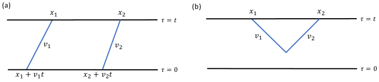
From the configurations in (a), we get:
| (121) |
From the configuration in (b), since we must have for the membranes to join together,
| (122) |
where we have used the constraints (4) to see that the quantity in (122) is minimized for . Minimizing between and , we see a linear growth of entanglement entropy followed by saturation at the thermal value:
| (123) |
For consisting of intervals , we have a minimization over a larger set of configurations, which leads to the following result
| (124) |
(124) is always non-decreasing as a function of time, in contrast to the evolution of multiple interval entanglement entropy in the integrable quasiparticle model [33].
To derive this formula for the Brownian models of this work, we need understand the structure of the “multi-particle” excitations involving more than one domain wall. We will understand this structure for the simplest case of from (36).
For an initial state with two or more domain walls, the action of can cause domain walls to annihilate in pairs, and it is useful to divide into parts and as discuss below (51). The action of on the multi-domain wall state , , is given by
| (125) |
when all . If any are such that , the action is such that we can simply delete the terms with any repeated appearing on the RHS of (125). The action of is
| (126) |
An initial state with zero or 1 domain walls is annihilated by .
Due to (125), eigenstates of take a simple non-interacting, free fermion-like form of (52) with energies given by the sum of the one-particle energies in (41), . Hence, the total propagator can be written as
| (127) |
where is the single-particle propagator defined in (43).
Consider the evolution of for a region consisting of intervals, . Expanding the evolution under in the interaction picture, treating as the interaction, we get
| (128) | |||
| (129) |
We can check from (126) that after insertions of at any intermediate times, the state necessarily gets annihilated, so that the interaction picture expansion truncates at (129). Using (127)and (126), together with the expression (46) for the domain wall propagator, we can show that the sum over the terms in (129) leads precisely to the minimization of (124) in the scaling limit.
Appendix D Variational approach for low energy excitations of
In the variational calculations discussed in this work, our goal can be stated as follows: we select some orthonormal basis of candidate states, , for some . We then consider a general state in the subspace spanned by , i.e., , and want to minimize the expectation value of some Hamiltonian with respect to the coefficients , subject to the normalization condition . It is easy to see that this minimization problem is equivalent to finding the lowest energy eigenstate of an “effective Hamiltonian” projected to the subspace:
| (130) |
The smallest eigenvalue of is the minimized expectation value in the given subspace, and the corresponding eigenvector corresponds to the optimal coefficients . The calculation shown in Appendix B.3 is a trivial version of this procedure.
For our Hamiltonian , we generally look for excitations of the form
| (131) |
It is natural to parameterize the excitations as plane waves due to the translation-invariance of . For a system with open boundary conditions, this is a natural ansatz in the thermodynamic limit. Taking the form of the excitations to be asymptotically towards the left and towards the right ensures that we are in the right sector of the Hilbert space for finding eigenstates of that contribute to the -th Renyi entropy of the left half-line. It also ensures that the states we consider have vanishing overlap with any of the ground states in the thermodynamic limit, so that the above minimization procedure will give an estimate of the lowest excited energy with the given momentum, and not the ground state energy.
Now for any given , we must find an appropriate orthonormal basis of states of the form (131). Let us start with the simplest non-trivial example of for of the GUE model, where , . In this case, the two options and span the whole relevant Hilbert space – the other two possibilities are redundant as the the resulting states differ from these cases only by an overall phase in the thermodynamic limit. However, note that the two states
| (132) | |||
| (133) |
are not orthonormal. To find in an orthonormal basis, we use the following two steps:
-
1.
We find the four matrix elements directly in the thermodynamic limit. This is easy to do due to the fact that , where is the nearest neighbor term in .
-
2.
We construct the gram matrix with matrix elements semi-analytically for a large value of and use it to construct an orthonormal basis for the subspace spanned by (132)-(133). In practice, is sufficient for the convergence of the coefficients of in the orthonormal vectors. We then transform found in point 1 to the orthonormal basis to find , which is simply a matrix in this case.
We then plot the lowest eigenvalue of obtained for each to obtain the curves in Fig. 6. The generalization of this procedure to higher for in the GUE model is straightforward. For the remaining cases of in the Brownian GUE model and of in the Brownian mixed field Ising model, again we use the same two steps Let us describe the case more explicitly in each case.
For the third Renyi entropy in the GUE model, we need to allow for arbitrary permutations in . A convenient way to form an orthonormal basis for this case is as follows. Let us label the one-site states associated with permutations other than and as , =1, …, 4. First, for each , subtract the components of the state along both and to get a state . Then find the orthonormal states , in the subspace spanned by . Then for the case, the relevant set of five states is
| (134) | |||
| (135) |
Note that we have not included the state with at , as this is redundant with the choice (134). The states (135) are already orthonormal among themselves, and orthogonal to . The normalization factor in has to be computed numerically, and converges to some constant for large enough . We can then find the matrix elements of directly in the thermodynamic limit.
For of (21) for the mixed field Ising model couplings in (82), we need to consider a 16-dimensional Hilbert space at each site. We can construct an arbitrary one-site orthonormal basis of states , , which are orthogonal to the permutation subspace spanned by . Then for , we can take the orthonormal basis to be
| (136) | |||
| (137) |
where again the normalization factor can be computed numerically for finite until it converges to some number, and the only remaining microscopic inputs needed to compute the matrix elements of in this basis directly in the thermodynamic limit are the two-site matrix elements such as , , and so on.
Appendix E Arguments using diagrammatic approach in the Brownian GUE model
E.1 Diagrams in interaction picture
In Sec. IV.1.3 of the main text, we used the structure of the eigenstates for any finite to argue that the domain wall propagator, defined as
| (138) |
is given by
| (139) |
where is the exact dispersion relation at finite , which we obtained numerically. In this appendix, we will use perturbation theory to understand the structure of the diagrams coming from in (36) that correct the large propagator from ,
| (140) |
The resummation of all such diagrams should in principle lead to the exact result (139). Note that we are now using “0” subscripts to denote , , and for which we found in Sec. IV.1.1, to distinguish them from the exact quantities appearing in (138). Quantitatively, the perturbation theory approach is much weaker than the numerical techniques discussed in the main text. In particular, the corrections that we obtain order-by-order in do not lead to membrane tensions that satisfy the constraints (4) well at finite . Moreover, this discussion only applies to , as the zeroth order Hamiltonian is gapless for . However, one advantage of discussing the diagrams is that they allow us to better explain the connection of our results to the diagrammatic approach used for circuit models in [38]. The diagrammatic approach in the interaction picture may also be more directly generalizable to higher dimensions than than the dispersion relation approach discussed in the main text.
Let us use the following expansion of the Euclidean time-evolution operator:
| (141) |
Putting this expansion into , the first term gives the bare propagator from the previous section. Recall that the action of sends a state with one domain wall to a state with three domain walls. For the second term in (141) to contribute to the domain wall propagator, two of the three domain walls created by the action of must annihilate at an intermediate time between and due to the action of defined in (126), see Fig. 17 (a). The resulting contribution to the domain wall propagator is
| (142) |
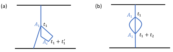
By inserting resolutions of the identity in the energy eigenbasis of before and after and , and doing the integrals over and ,
| (143) | |||
| (144) |
where was defined in (52), and is defined such that
| (145) |
In the final expression (143), we have kept only the leading linear-in- term in the large limit, ignoring the and exponentially suppressed terms. This leading contribution comes from the regime in the diagram Fig. 17 (a) where is . (The proportionality to in the second term of (143) comes from the fact that the small bubble of size can be placed at any value of from 0 to .) By summing over the leading contributions at large from the series of diagrams in Fig. 18, the correction in (143) exponentiates to
| (146) |
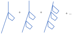
Similarly, one can check that the leading correction at large from the diagram in Fig. 17 (b), which comes from the third term in (141), is
| (147) |
and exponentiates to give a correction in the energy. In all, these “renormalize” the bare dispersion to , where
| (148) |
By extending the same reasoning to higher order terms in the expansion (141), we can see that the exact dispersion relation at finite is a resummation of the full set of diagrams in the interaction picture where we have departures from the one domain wall subspace into the multiple domain wall subspace for an amount of time at intermediate times. These are precisely analogous to the diagrams considered for circuit and Floquet models in [38]. Note that the corrections and to the dispersion relation found above can also be independently derived by using a version of Schrodinger picture perturbation theory adapted to the non-Hermitian starting point .
In the next subsection, we will use a thickened line to denote the exact propagator of (139) at finite , which should now be understood as a sum over the following set of diagrams for departures from the one domain wall subspace:
![[Uncaptioned image]](/html/2407.16763/assets/x29.png)
E.2 Argument that configurations where the domain wall splits are subleading for any initial state
Under the action of the full Hamiltonian in (36), a single domain wall state can evolve to a state with an arbitrary number of domain walls, so that (44) for the large limit should be replaced with the following expression for the exact evolution at finite :
| (149) |
where we have inserted a resolution of the identity in the subspace of odd numbers of domain walls to the right of . Note that for instance .
Using the interaction picture diagrams of the previous section, can be expressed as follows in terms of the exact propagator , again up to an overall prefactor which does not have an exponential dependence on :
| (150) |
This gives the following contribution to (149), which can be represented by a sum over diagrams shown in Fig. 19 (a) (for now, let us ignore the dashed line in the figure):
| (151) |
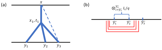
If we have a pure product initial state such that the initial value of for any region is zero, then it is immediately clear that any such contributions where the domain wall splits are exponentially suppressed in time compared to the first term in (149). Even taking into account the contribution from an arbitrary initial state, we can use the convexity of the membrane tensions obtained in Fig. 7 to show that the first term of (149) dominates, as follows.
Let us fix some arbitrary set of positions . Consider an initial state that is maximally mixed in the region , and has maximal entanglement between the degrees of freedom in and the degrees of freedom to the left of . See Fig. 19 (b). For this state, the initial entropy contribution in (151) is minimized for .
Let us now consider the total potential contribution to the from the diagram in Fig. 19 (a) with for this initial state:
| (152) |
Let us now compare this contribution to the single domain wall configuration shown with the dashed line (coming from the first term of (149)), which contributes
| (153) |
Now using the convexity of ,
| (154) |
and by similar steps to those leading to (122), by making use of the constraints (4),
| (155) |
We therefore find that always wins in the minimization problem in the scaling limit. It is clear that if wins even for this choice of initial state, it will also be the dominant contribution for any other choice of initial state.
Appendix F Operator growth interpretation of domain wall splitting
Consider a basis of operators for a single site, , such that , and satisfying . By taking tensor products of these operators, we can also construct a basis of operators for the full system, satisfying
Let us introduce the two-copy states associated with these operators, such that . In terms of these states, the four-copy spin states defined in (34)-(35) can be shown to be written as
| (156) | |||
| (157) |
It is natural to introduce the notion of a probability that some initial operator in the full system evolves to some final operator under the unitary evolution [73, 74, 14, 15]:
| (158) |
Using (156), for any initial operator and some position in the system, we define as
| (159) |
where “ ending to the left of ” means that the is equal to the identity for all sites to the right of . This is the total probability that the operator evolves to an operator that has support only on the left of . Now consider two different kinds of initial operators from the basis ending at some point (meaning that has a non-trivial operator at , but is equal to the identity everywhere to the right of ). One type of operator has non-trivial operators at all sites to the left of , while the other is equal to the identity at some and nontrivial at all other . Consider the quantity , where
| (160) |
where denotes the average over all basis operators with the property described in the subscript. Using (157),
| (161) |
In random unitary circuits, since a single domain wall does not split, we have , indicating that the evolution of the endpoint of an operator is independent of its internal structure, which is consistent with a maximally random time-evolution. In the Brownian GUE model, is highly suppressed at late times, but non-zero, indicating that there is some slight sensitivity of the operator growth to the internal structure. However, such effects do not modify qualitative features of the dynamics such as the validity of the membrane picture for the second Renyi entropy.