382 Via Pueblo, Stanford CA 94305
APD-Invariant Tensor Networks from Matrix Quantum Mechanics
Abstract
We propose a simple connection between matrix quantum mechanics and tensor networks. This allows us to imbue tensor networks with some interesting additional structure. The geometry of the graph describing the tensor network state is determined dynamically, giving a notion of background independence. The tensor network states have a invariance, which (a) allows us to consider continuous families of entanglement cuts even with a finite number of tensors and (b) includes a notion of bulk coordinate reparameterization and area-preserving diffeomorphism invariance in the large limit. These tensor networks also have a natural scale of nonlocality that behaves similarly to a string scale, suggesting a potential toy model for sub-AdS physics. Emergent gauge fields naturally appear on the tensor network links.
1 Introduction
Following the second superstring revolution schwarz1987review ; polchinski1996tasi a family of holographic dualities was proposed between large quantum theories and various corners of string theory banks1999m ; Maldacena:1997re ; itzhaki1998supergravity ; berenstein2002strings ; gubser1998gauge ; witten1998anti . These dualities share a heart – their quantum mechanical sides are generically worldvolume theories of some stack of D-branes in the decoupling limit. The most well-studied example is the gravitational theory emergent from dimensionally reduced 9+1d Super Yang-Mills (SYM) Maldacena:1997re ; itzhaki1998supergravity . The worldvolume theory of D3-branes in particular is conformal, and the emergent spacetime is string theory in AdS Maldacena:1997re , so the case is a particular instantiation of the more general AdS/CFT correspondence. However, following the general arguments of t1993planar , even non-conformal large- theories in the appropriate limit often define some emergent string theory.
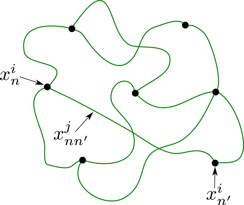
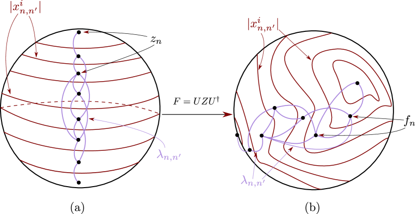
In this paper we focus on matrix quantum mechanics (MQM), in which the ‘boundary’ theory is neither conformal, nor a QFT, but a quantum mechanical system with a finite number of degrees of freedom living on a 0+1 dimensional base space. The BFSS banks1999m and BMN berenstein2002strings models are particular examples of type IIA string theory emergent from interacting D0-branes. The degrees of freedom consist of Hermitian matrices and fermionic matrices . The entries of these matrices are denoted and , with the color indices running from 1 to . When considered as the worldvolume theory of D0-branes, the eigenvalues of the matrix are interpreted as the positions of the branes along the th spatial dimension and the off-diagonal elements as modes of strings stretching between the th and th branes polchinski1996tasi . See Fig. 1(a) for a diagram. As before, MQM Lagrangians with stringy duals have the schematic form of dimensionally reduced SYM:
| (1) |
The commutator squared term may be recognized as the zero-mode piece of the covariant SYM derivative. It is precisely this term that is responsible for imbuing strings with a potential energy linear in their length (see taylor2001m for a review).
Since the discovery of holographic duality, there has been a concerted effort to develop tractable toy models that capture important aspects of its physics. Tensor networks pastawski2015holographic ; Hayden:2016cfa ; swingle2012entanglement have been one of the most celebrated and fruitful of these models, and particularly excel in capturing the emergence of bulk geometry from quantum correlation in the boundary theory. Among other phenomena they capture holographic error correction, bulk reconstruction, the Ryu-Takayanagi formula for boundary entropy ryu2006holographic , and a notion of sub-AdS locality yang2016bidirectional . Suprisingly, they have even recently been shown to recover bulk gravitational forces that appear to directly arise from the entanglement pattern Sahay:2024vfw . They are essentially lattice-regularized holography.
The key building block of of a tensor network is a generic state on qudits with Hilbert space dimension . The most general such state is described in terms of a multilinear operator (i.e. tensor) :
| (2) |
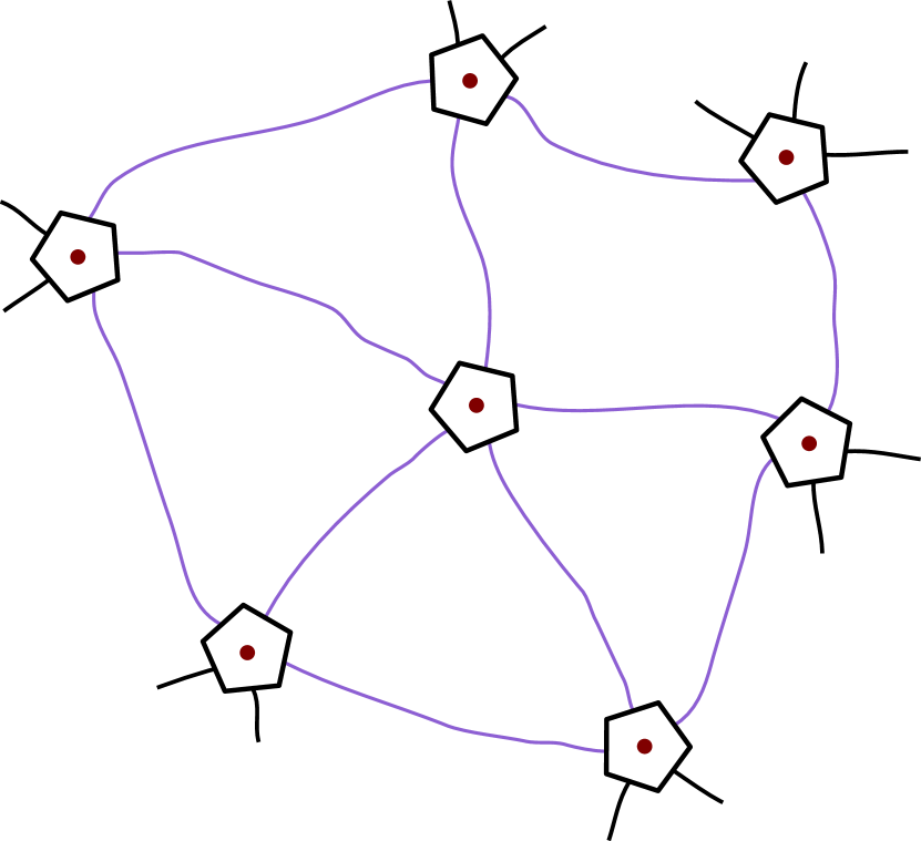
These states are pictorially represented as a geometric shape with external legs, with one qudit associated to each leg (see Fig. 1(b) for an example). General tensor network states are built by entangling qudits on the external legs of different tensors. This is done by taking inner products of the tensors . To represent entangled qudits, we connect the legs of the tensors to form an internal edge. As such, tensor network states are graphs (again, see Fig. 1(b)).
While they successfully capture many aspects of AdS/CFT, tensor networks suffer from deficiencies. As they are defined on a lattice determined by some graph, they lose the diffeomorphism invariance and background independence that constitute general covariance of the bulk geometry (see Akers:2024wab for an alternative recent approach for introducing diffeomorphism invariance using the Chern-Simons description of 3d gravity). It is further unclear how tensor networks properly describe the backreaction of RT surfaces on the geometry Dong:2023kyr ; Akers:2024wab . While capable of probing some sub-AdS lengthscale physics, they do not capture corrections and the UV/IR mixing we expect from physics at the string scale.
In this paper we argue that MQM states are naturally thought of as a generalization of tensor network states. The construction is built on a simple observation – the Hilbert space of MQM is identical in structure to the Hilbert space of tensor networks. Moreover, the matrices defining compact noncommutative manifolds have a natural interpretation as graph adjacency matrices. Mapping tensor network states into invariant MQM models allows us to define tensor networks on noncommutative manifolds. The symmetry in the large limit contains area-preserving diffeomorphisms (APDs) hoppe1982quantum (see swain2004topology for discussion of some subtleties on this point), and a judicious choice of Hamiltonian allows the background geometry to be determined dynamically, so we may think of this construction as a step toward introducing general covariance and background independence into tensor network models. This construction may be viewed as a particular instantiation of the ideas in Cheng:2022ori .
1.1 Overview of the Construction
The construction in this paper relies on results and intuition from tensor networks, noncommutative geometry, and noncommutative field theory. For the convenience of a reader that may unfamiliar with one or more of these concepts we give a brief sketch of the core idea, where we give the essential results but leave their technical justification for §3.
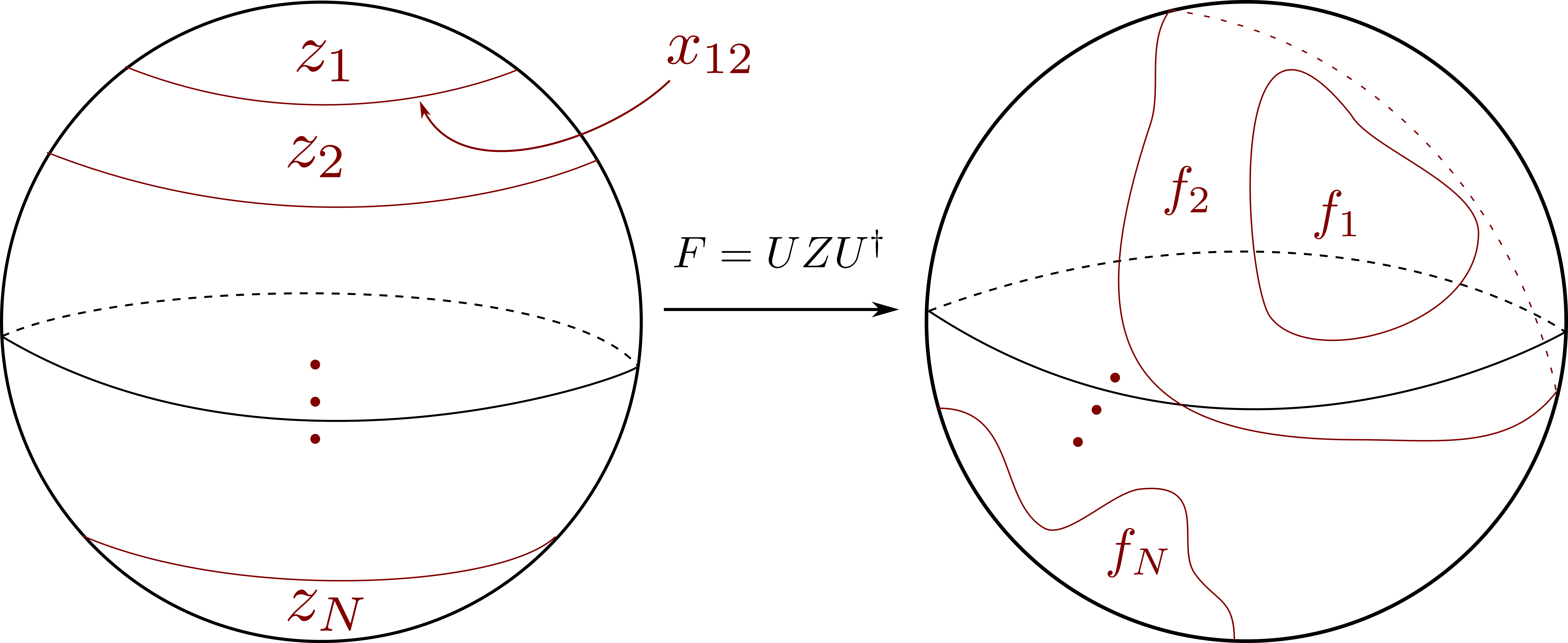
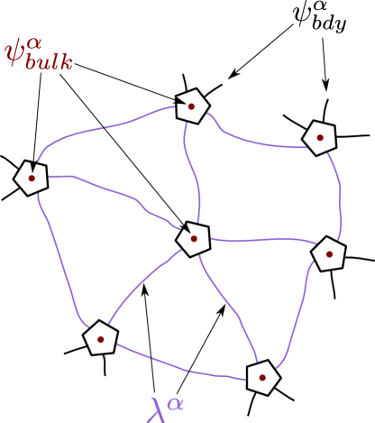
As we review in §2, a noncommutative manifold is defined via a set of matrices . The are the generators of the algebra of functions on , and are themselves interpreted as the coordinate functions. One of the observations of §2 is that carry a natural interpretation as the adjacency matrices of a graph. For similar observations, see Hampapura:2020hfg ; Frenkel:2021yql . An example of such a graph in the case of is drawn in Fig. 2.
We wish to put a tensor network on this graph in a manner that respects the coordinate reparameterization symmetry of noncommutative manifolds. To do so, we introduce matrices of qubits . is a flavor index that runs from to . Our total Hilbert space therefore consists of the and degrees of freedom, and there is a natural adjoint action of the symmetry group on this Hilbert space. The explicit generators of this action are given in (21). In view of Fig. 1(b), maximally entangling the qubits with the qubits creates a link between the th and th nodes.
The key to the construction is how we determine the state of the tensor network. We write -invariant MQM Hamiltonians on the and degrees of freedom and consider their low energy states. While we expect the relationship between MQM and tensor networks to be quite general, for simplicity the specific Hamiltonians we consider in this paper take the form
| (3) | |||
| (4) | |||
| (5) | |||
| (6) |
is the Hamiltonian that sets the geometry of the noncommutative manifold. It consists of a kinetic term (the are the conjugate momenta of the ) and a potential term . This could be something like mini-BMN Anous:2017mwr ; Han:2019wue , which has the fuzzy sphere as a ground state. is designed to maximally entangle all qubits with their counterparts. controls the strength of the backreaction of the fermion modes on the geometry. For the purposes of this paper we work in the regime of , so as not to worry about this backreaction.
The ground state of is an all-to-all connected tensor network graph. is the coupling between the geometry and the tensor network qubits. On its own, the ground state of is the completely unentangled state of all the qubits – without , this would define a completely disconnected network. The commutator structure has a nice interpretation in the noncommutative geometry – the commutator is the noncommutative analog of the Laplacian . We should therefore read as
| (7) |
where the couplings set a derivative expansion in the Hamiltonian of some spinor fields propagating on . The structure of suppresses high momentum modes of , and by tuning we may set a momentum scale for modes that can propagate in the low-energy subspace of (3). The nature of noncommutative geometry is that momentum scales are related to length-scales – high momentum modes spread out in the transverse directions to the direction of propagation McGreevy:2000cw . By setting a momentum scale, we also set a length-scale across which internal edges of the tensor network can stretch. This is the scale of nonlocality of the network. The competition between and is what sets the scale of nonlocality and creates the local entanglement strucure of the states we consider.
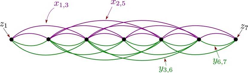
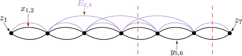
It is crucial that the Hamiltonian of (3) is invariant, so that we may restrict ourselves to the subspace of -invariant states (i.e. we may gauge this symmetry111In quantum mechanics, as opposed to quantum field theory, we often have a choice about whether or not to take a symmetry to be global symmetry or a gauge redundancy. It is only a question of whether we restrict to the subspace of the Hilbert space annihilated by the symmetry generators.). So far, as depicted in Fig. 3, we have described tensor networks where each node has a fixed coordinate. It may seem that this only allows us to partition our network along . However, by acting with a unitary transformation on the and matrices, we may transform the state of our tensor network to a new basis that admits a Hilbert space factorization along any curvilinear coordinate222There is a UV cutoff on the curvature of coordinates we may consider given by , the scale of noncommutativity. However, it is important to note that unlike a standard tensor network, we may consider continuous families of coordinates (and therefore a continuous families of entanglement cuts). of our choosing (see Fig. 4).
A punchline here is that in the large limit, area-preserving diffeomorphisms are a gauge symmetry of these matrix tensor networks. Different gauge fixing conditions behave as different coordinate systems on , and each coordinate system presents us with a different coordinate along which we may partition the network and compute an entanglement entropy (again see Fig. 4). It is quite nontrivial that the ground state of (3) has area-law entanglement for any choice of entanglement cut333The cut should be weakly curved compared to the scale of nonlocality we introduce in §§1.2.. This is the main technical result of this paper and what is shown in §§3.3.2.
1.2 A Planck Scale and a String Scale
The holographic bulk of D-brane systems has three essential length-scales444More precisely, two independent unitless ratios of length-scales. – the scale of the geometry (i.e. the AdS radius) , the string scale , and the Planck length . The string scale in particular is the scale of nonlocality – the Ryu-Takayanagi formula picks up corrections as extremal surfaces become more and more curved Dong:2013qoa ; Wall:2015raa , and we expect that the area law contribution will cease to dominate below the string scale. In Maldacena:1997re ; itzhaki1998supergravity , it is emphasized that the ratios of these length-scales are given by
| (8) |
is the ‘t Hooft coupling, and sets the string scale in the bulk. In the holographic dualities considered in Maldacena:1997re ; itzhaki1998supergravity and related works, the ‘t Hooft coupling (and therefore the ratio between the string scale and the AdS length-scale) is in scaling. The Planck length , meanwhile, is separated from the AdS lenghtscale and the string scale by nontrivial factors of .
The tensor networks we consider naturally impose on us three length-scales that have a behavior strikingly similar to those in (8). Consider Figs. 3 and 4, and call the size of the geometry . One natural length-scale to consider is the typical separation between nodes of the network, or equivalently between D0-branes in Fig. 1(a). This is analogous to – it is the shortest possible distance scale, and sets the total number of degrees of freedom. The other length-scale is the typical lengths of the tensor network edges – the purple edges in the two figures. They need not only connect nearest-neighbor nodes, and may in principle stretch long distances along the geometry. This is the scale of nonlocality of the network, and behaves similarly to the string scale . We refer to these scales as and respectively. The ratio of these two length-scales is set by the structure of in (3), and in particular by the strength and structure of the couplings in the derivative expansion.
Note that in light of the D0-brane origin of holographic MQM (as in Fig. 1(a)), the interpretation of this scale of nonlocality as a string scale might be taken quite literally. Below this scale, the off-diagonal matrix elements and modes connecting branes arehighly excited and entangled with nearby degrees of freedom. Above this scale, and are suppressed to their ground states. This exactly matches the behavior of off-diagonal matrix elements (i.e. string modes connecting branes) in D-brane matrix quantum mechanics taylor2001m ; Polchinski:1999br .
To find the nice property that area law entanglement is simply given by the number of tensor network legs crossing a given entanglement cut, we find in §3 that we must consider the regime
| (9) |
In particular, the ‘string scale’ must be much greater than the ‘Planck scale’. It is perhaps an interesting coincidence that this regime includes the analog of the ‘t Hooft limit. The string scale of the matrix tensor networks we define depends on the Hamiltonian we choose, and we will find area law entanglement only above the string scale we set.
1.3 Layout of the Paper
In §2 we review the relevant main ideas of noncommutative geometry. We also argue that the matrices representing the noncommutative coordinate functions have a natural interpretation as the adjacency matrices of a graph.
§3 contains the main results of the paper. We embed the structure of tensor networks into the MQM Hilbert space. We find that these noncommutative tensor networks have a natural scale of nonlocality, mimicking a string scale. This string scale may be tuned arbitarily small in comparison to the size of the geometry in the large limit, similar to the limit of strong ‘t Hooft coupling. We show that the low-energy states of reasonable -invariant MQM Hamiltonians produce states with area-law entanglement above this string scale, demonstrating that local geometry may emerge dynamically for these models.
In §4 we discuss the results and comment on future directions.
2 Fuzzy Coordinate Functions as Adjacency Matrices
Noncommutative geometry has a storied history within string theory in general seiberg1999string ; douglas2001noncommutative ; szabo2003quantum ; witten1986non ; Ardalan:1998ce and matrix quantum mechanics in particular taylor2001m ; Steinacker_2010 ; Steinacker:2011ix ; Han:2019wue . The bulk of holographic systems, especially the compact dimensions, exhibit phenomena similar to physics on noncommutative backrounds McGreevy:2000cw ; ho2000large ; ho2001fuzzy . In this section we briefly review how noncommutative manifolds are defined and how they naturally emerge in MQM systems.
Noncommutative manifolds (which we denote ), much like their commutative counterparts, are defined through their algebra of functions and metric structure. The essential aspect is that the coordinate functions parameterizing do not commute, and instead obey some relations
| (10) |
The algebra of functions on is then generated by all sums and products of the . Perhaps surprisingly, from this basic starting point we may introduce a differential and integral structure. Consider some function on . Its derivatives are given by
| (11) |
This definition is particularly natural because commutators obey the Leibniz rule. The Laplacian, which in turn determines the metric structure, is defined as
| (12) |
Integrals are given by traces –
| (13) |
The simplest way to work with noncommutative manifolds is by finding a representation of their algebra. The prototypical example is the fuzzy sphere, which is defined by the relations
| (14) |
We recognize these expressions as the defining relations of representations, and may find an explicit realization of the fuzzy sphere by choosing an irrep of –
| (15) |
This is the basis in which is diagonal and its eigenvalues are ordered. We interpret the spectrum of as the distribution of -brane positions over the axis. That the eigenvalues are evenly spaced is a signature of the commutative sphere measure being .
With an explicit representation given by matrices, there is a close relationship between derivatives and length scales. In particular, consider some function on a noncommutative manifold represented by a matrix with entries . Its commutator with a diagonal coordinate matrix (say ) is
| (16) |
The ratio therefore measures the typical distance between coordinates that elements of stretch between, weighted by the size of the elements . By extension, the noncommutative gradient measures the average length squared of the matrix elements excited in , and therefore sets a length-scale for .
In the basis where is diagonal, and are sparse matrices with support only on the diagonals adjacent to the main diagonal. This means that e.g. in Fig. 5, is only nonzero in a particular basis if and are adjacent D0 branes in the coordinate system corresponding to this basis. In this sense, and precisely behave as adjacency matrices of a graph. Digging a bit deeper, is precisely the length of the perimeter between the th and th D0-branes. The reason for this is that projection matrices are the noncommutative analog of step functions, and their derivatives (the natural noncommutative analog of a delta function) pick out the off-diagonal blocks of the coordinate matrices .
So far we have taken the coordinate functions to be fixed. One way in which noncommutative geometry naturally arises in MQM is by interpreting the dynamical Hermitian matrices in (1) as the coordinate matrices of a noncommutative manifold . Because the metric structure is determined by the , if we make the fuzzy coordinates dynamical we also make the metric dynamical. The fuzzy sphere, for example, arises as one possible vacuum state in the BMN (or mini-BMN Han:2019wue ; Anous:2017mwr ) matrix model. (1) is precisely designed to energetically suppress string modes propagating between distant D-branes, and we can see this effect explicitly from (14) in that only the matrix elements between adjacent D-branes are populated with nonzero entries. In this way, it is natural for low-energy states of MQM models to behave as dynamical adjacency matrices of local graphs that only have connections between nearby nodes. Because the geometry and topology of these graphs are determined by the dynamics of the theory, they come with a manifest sense of background independence.
Intuition tells us that in low energy states of quantum systems degrees of freedom which are more strongly coupled are more entangled. Moreover, it is often tempting to interpret strings stretching across an entanglement cut as extended degrees of freedom which should be cut to produce entanglement edge modes Susskind:1994sm ; levin2006detecting ; ghosh2015entanglement ; hampapura2021target ; Frenkel:2021yql ; frenkel2023emergent . The way in which we make this intuition precise is by interpreting the graph arising from the adjacency matrix picture of as the graph of a tensor network. This is the task we take up in §3.
2.1 Subregions of Noncommutative Manifolds
Considering subalgebras and entanglement on the tensor networks we are defining is closely related to the idea of considering geometric subregions of noncommutative geometries. On a typical commutative manifold, a subregion is defined via a characteristic function . evaluates to 1 inside and evaluates to 0 on the complement . Any function may be decomposed into two parts:
| (17) |
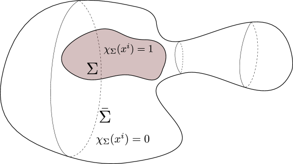
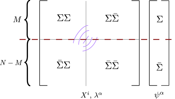
On a noncommutative manifold characteristic functions are promoted to projection matrices satisfying . Unlike the commutative case, a noncommutative function has four distinct pieces to consider:
| (18) |
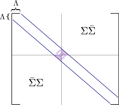
If we choose a basis where is diagonal with ordered eigenvalues, this is nothing more than a block decomposition of the matrix (see Fig 7). The blocks and are associated to the boundary of the noncommutative manifold, and in particular should be thought of as modes that cross the boundary (see Fig. 8).

To consider RT surfaces, instead of minimizing over a discrete set of entanglement cuts we must minimize over the continuous set of projection matrices. This type of minimization will appear shortly in ffhs:2024xx , and would be interesting to directly apply to entropy calculations and bulk reconstruction in the tensor networks we are considering.
3 Embedding Tensor Networks into MQM
3.1 The Embedding Map
We interpret the color indices of the matrices as nodes in the network. To construct quantum states, we introduce dynamical degrees of freedom in the form of matrices of spinors and vectors of spinors . For simplicity, instead of treating these spins as fermions we take their (anti-)commutation relations to be
| (19) |
We take this unusual choice to simplify the representations of the operators, so that we may take e.g.
| (20) |
With these conventions, the generators of transformations on the , , variables take the form
| (21) |
The creation operators act on the dimensional Hilbert space that lives on the link connecting nodes and . On each factor of the Hilbert space, we label as the states annihilated by and the states annihilated by . We interpret the dynamical variables as living on ‘external’ legs of the tensor network with corresponding spaces . For holographic models these can be interpreted as either boundary or bulk external legs, depending on where the node is located in the fuzzy geometry. For notational convenience we introduce a basis of states or on the corresponding Hilbert spaces, with the index running from 0 to .
We have now introduced all the degrees of freedom necessary to construct any tensor network state depending on what state we fix on the products . For the most straightforward type of network, we can create a link (or a lack of a link) between the nodes and by choosing one of two states on these spaces:
| (22) |
Of course, as Hayden:2016cfa ; Cheng:2022ori point out, it is fruitful to consider more general types of connections between nodes besides maximally entangled states. With this in mind, we generally take a state in as defining the graph the tensor network lives on, so we denote elements of as .
To introduce random tensor networks, random tensors are defined on the states
| (23) |
Correspondingly, given a ‘graph state’ the state on the external links is given by
| (24) |
3.2 Partitions and Subalgebras
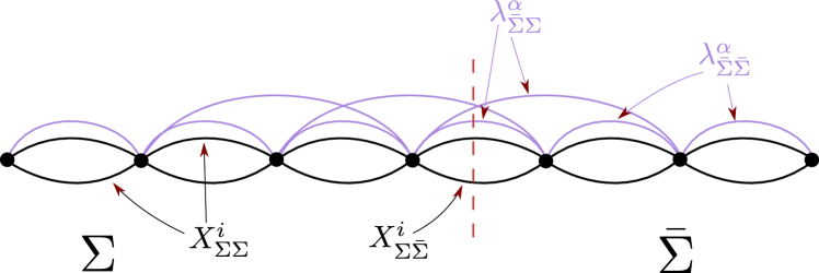
Now that we have described the Hilbert space of the theory (22), we explain how to consider subregions of MQM systems and matrix tensor networks in particular. This story is essentially the same as that of target space entanglement in MQM das2020bulk ; Das:2020jhy ; karczmarek2014entanglement ; hampapura2021target ; Han:2019wue ; frenkel2023emergent ; Frenkel:2021yql , but contains a crucial unique ingredient in how we treat the off-diagonal matrix elements.
Remember that each matrix entry has a Hilbert space associated to it. This is true of both the and the . The essential idea, then, is to choose an appropriate basis in which to write our vectors and matrices555This should be thought of as a gauge fixing condition for our invariant wavefunctions. and split the system along the row index (see Fig. 10). More precisely, we write
| (25) |
The most convenient way to split a matrix is to introduce a projection matrix on color space. The label may be associated to a subregion of the noncommutative manfiold of area (see §§2.1). is the noncommutative analog of a characteristic function, which evaluates to 1 on some subset of a manifold and evaluates to 0 on the complement of .
3.3 Dynamically Introducing Locality
Thus we have introduced the tools to in principle describe tensor networks on potentially all-to-all connected (or otherwise nonlocal) graphs. To make contact with the typical notion of tensor network, however, we want there to be a sense in which only nearby nodes are connected. We could by hand choose a graph state that reproduces a local network, but this simply reduces us to the construction explored in Hayden:2016cfa . In this section consider some simple MQM-like Hamiltonians and argue that their low-energy states have the properties of tensor networks with only geometrically nearby nodes connected.
We consider two classes of MQM models. The first are based on Matrix Quantum Hall models Susskind:2001fb ; Hellerman:2001rj ; Polychronakos:2001mi ; Tong:2015xaa where there are two coordinate matrices and that commute at a classical level but not as quantum operators. This is the usual way by which noncommutative geometry arises in quantum hall models, as and become conjugate phase space variables in the limit of a strong magnetic field. We refer to this setup as classically commutative, quantum noncommutative, and explore it in §3.3.1. This is the notion of noncommutative geometry considered in e.g. Zhu:2022gjc .
The second class consists of field theories on honest noncommutative geometries with classically noncommuting coordinates. We refer to this as the classically noncommutative setup and discuss it in §3.3.2. This setup has a much richer structure and is closer in spirit to MQM with multiple matrices.
3.3.1 Classically commutative, Quantum noncommutative geometries
As in Polychronakos:2001mi ; Tong:2015xaa we consider a complex matrix . We make the assumption that , so that is unitarily diagonalizable. We first consider the case where the matrix is fixed and has eigenvalues . For simplicity, we drop the index on the and spinors for now. The Hamiltonian we consider is
| (26) |
We choose to work in a basis where is diagonal. In components, this Hamiltonian is written as
| (27) |
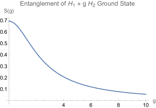
This Hamiltonian decouples on each Hilbert space factor , where each is two dimensional. The ground state of is the maximally entangled state . The ground state of is . The entanglement of the ground state of as a function of the coupling is
| (28) |
Its behavior is shown in Fig. 11, but the only important point about its functional form is that it is for and falls off as for . The overall ground state wavefunction will simply be a tensor product of the ground states of each .
So far we have not moved beyond familiar tensor network graphs. To do so, we introduce dynamics on . We take the Hamiltonian studied in Polychronakos:2001mi ; Tong:2015xaa , which we refer to as the matrix quantum hall (MQH) model.
| (29) |
The matrix elements of obey the commutation relations
| (30) |
so without the coupling to the system decomposes into variables obeying the harmonic oscillator algebra.
We treat the system by passing to a collective field description, where we define the eigenvalue density
| (31) |
In terms of the Hamiltonian takes the form666I would like to thank Laurens Lootens for pointing out the similarity to continuous tensor network models as in Tilloy:2018gvo . One may view this construction as a fuzzy-regulated version of a continuous tensor network.
| (32) |
We have introduced an additional coupling constant , which we may take to be small to ensure the bilocal fields do not strongly backreact on the geometry. Each mode now decouples, and the entanglement of a subregion with its complement is now calculated to leading order in as
| (33) |
Noting that we may plug into (28) , falls off as
| (34) |
With this in mind, the integral in (33) is dominated by the UV contribution localized to the entanglement cut, so we find an area law entanglement.
3.3.2 Classically noncommutative models
We turn to a case where the background geometry on which the tensor network lives is honestly noncommutative at a classical level, as in §2. For clarity and concreteness we focus on the fuzzy sphere as in (14) Madore:1991bw , but the results of this section are readily extended to any weakly curved noncommutative geometry with small noncommutativity parameter.
We first consider the case where the background geometry is fixed, so the don’t fluctuate. The Hamiltonian on the degrees of freedom takes the form as in (3)
| (35) |
Sums over the repeated indices are implicit. As in §§3.3.1, we have dropped the index as it just comes along for the ride. The ground state of (35) is again easy to determine, this time by decomposing into matrix spherical harmonics Taylor:1999qk ; Han:2019wue :
| (36) |
The entanglement between the mode and the mode (for ) is obtained by plugging in the place of in (28).
It is most instructive to analyze this system in the diagonal basis, where is only supported on the th diagonal (see Fig. 12). It is clear from the structure of (36) that the fermion mode will only be entangled with the mode. Because the matrix entries of matrix spherical harmonics are a discretization of the usual commutative spherical harmonics , we may evaluate traces of products of the in terms of integrals of up to corrections suppressed by .
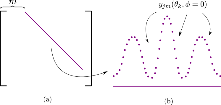
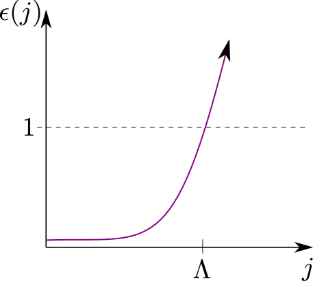
The entanglement structure of the ground state depends on the structure of . Modes for which is small will have large entanglement, and vice versa for modes for which is large. We take to have a form depicted in Fig. 13: it is a growing function of that sharply transitions from much less than 1 to much greater than 1 at some cutoff . As is standard on noncommutative geometries, a momentum scale is also a length-scale (see the discussion below (16)). Physically, is the length-scale of extended objects which propagate along the fuzzy sphere geometry. As such, it is the scale of nonlocality of the theory, and we refer to it as the string scale. To ensure a local entanglement structure for our network we take .
Unlike in §§3.3.1, there are two distinct contributions to the entanglement structure of the ground state. couples (and therefore entangles) the and matrix spherical harmonic modes, whereas couples entries of modes along the diagonals pictured in Fig. 12. To make contact with standard tensor networks, we wish for the former contribution to dominate. We do this by estimating the scaling of these two contributions in and .
The first issue is that the modes are delocalized across the sphere. In view of Fig. 12, we look for a fourier-like transform that takes the delocalized form of spherical Harmonics along the matrix diagonal into a more local form. For a particular cutoff , the th diagonal will have activated modes entangled with the opposite diagonal. There are lattice sites along the th diagonal, so we may squeeze each qudit to occupy lattice sites. The order of magnitude of the number of entangled qudits within the off-diagonal block (i.e. the number of cut tensor network edges contributing to the entanglement as in Fig. 14) therefore scales as
| (37) |
On the other hand, the number of diagonals with excited degrees of freedom that cross the entanglement cut simply scales as . This contribution to the entanglement is precisely what is computed in karczmarek2014entanglement , and scales as . As we take , note that we are within the area law regime found karczmarek2014entanglement . We therefore wish to take the limit . In order to for the scale of nonlocality to be much smaller than the scale of the background geometry, we must take . We therefore consider the parameter regime
| (38) |
To evaluate the entanglement, we simply need to rotate to a basis where induces a block decomposition of the matrix as in Fig. 10 and count the number of qubits in the block that are entangled with their partners in the block. This is given by the sum
| (39) |
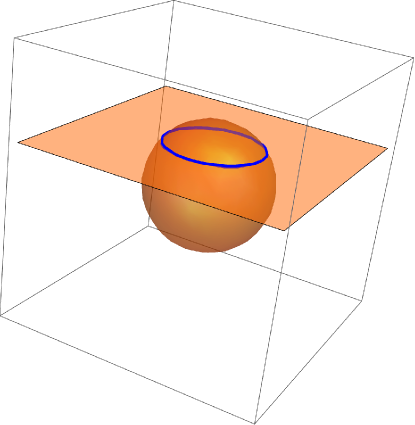
As an instructive example we explicitly evaluate this sum in a simple the simple case where is a cap subregion on the sphere (see Fig. 15) so that is diagonal in the same basis as . The spherical harmonics then take the form drawn in Fig. 12. The sum may be rewritten as
| (40) |
As the form a complete basis for matrices, we may expand the matrix itself in terms of spherical harmonics:
| (41) |
Via the Moyal map Moyal:1949sk ; Susskind:2001fb ; Steinacker:2011ix (and as strongly suggested by Fig. 12) we may approximate up to corrections as
| (42) |
The coefficients are therefore simply determined by the properties of the Fourier decomposition of step functions. In particular, for large they have the structure
| (43) |
is the lengthscale of the radius of curvature of . Put simply, the projection of a characteristic function onto high-momentum (compared to the radius of curvature) fourier mode subspaces has magnitude proportional to the surface area (i.e. perimeter for the case). For the case of the cap subregion symmetry demands that only is nonzero, so we simply have
| (44) |
Plugging this back into (39) we find
| (45) |
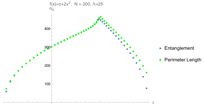
Taking large, we find that the number of tensor network legs partitioned by the entanglement cut is proportional to the perimeter length . As the entanglement is proportional to , we find area law entanglement in this parameter regime.
We may extend this argument to more general subregions using the techniques of Frenkel:2023yuw . Instead of we diagonalize some other matrix (as in Fig. 4), and take the radius of curvature to be given by . It is important to take . This matrix corresponds to the curvilinear coordinate on the sphere, along with an orthogonal curvilinear coordinate which satisfies . The computation was easy in the case of the cap subregion because spherical harmonics are eigenstates of . Because high-momentum spherical harmonics have the structure of plane waves on the surface of the sphere, we may find local rotations of the spherical harmonics that satisfy
| (46) |
such that is an eigenfunction of . This definition may be promoted to the fuzzy sphere by promoting the to be functions of the . The then get promoted to matrices that satisfy
| (47) |
This implies that now have the exact structure depicted in Fig. 12.
We now recall that the matrix commutator becomes the Poisson bracket on the fuzzy sphere surface. We therefore have
| (48) |
as the terms that dominate the Poisson bracket are those where the derivatives hit the instead of the . Pulling this back to matix expression in turn implies
| (49) |
Using this expansion we may now run the exact same computation as before, finding again the result (45) with the same overall numerical coefficient:
| (50) |
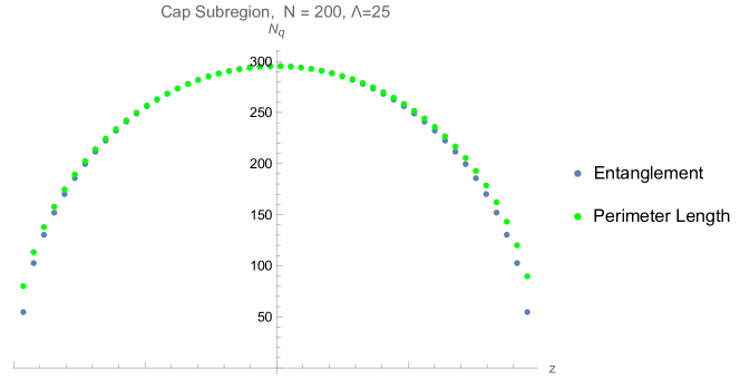
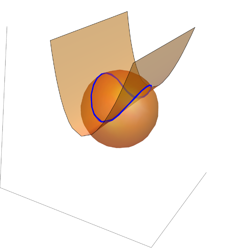
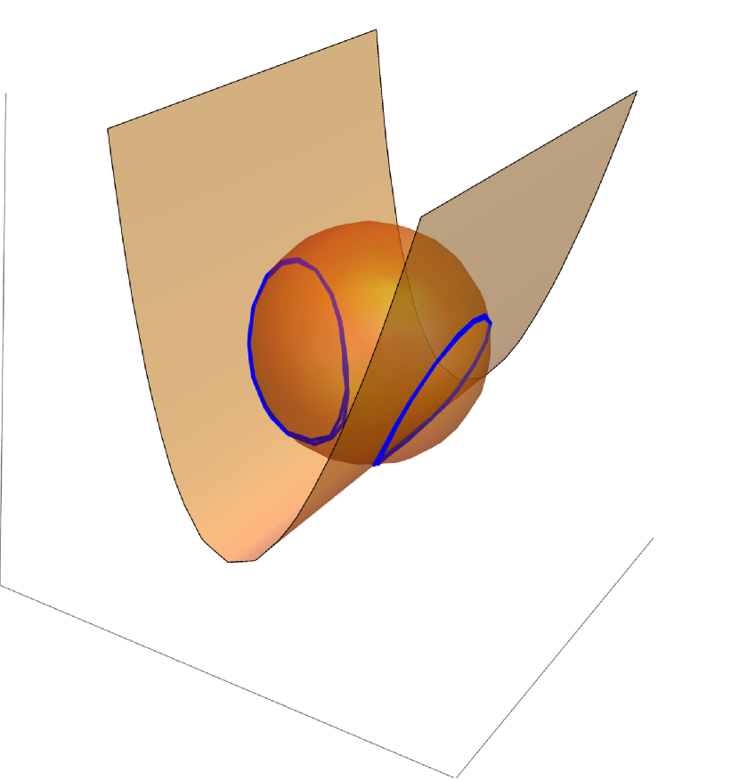
To help the reader trust these quick noncommutative function manipulations, we present numerical results. See Fig. 16 for a direct numerical evaluation of (39) for the cap subregion that confirms the area law behavior. See Figs. 17 and 18 for numerics for another family of entanglement cuts that includes topologically nontrivial subregions.
3.4 Emergent Non-Abelian Gauge Fields on the Links
The observation that tensor networks may incorporate emergent bulk gauge fields living on their links is nothing new Dong:2023kyr ; Akers:2024ixq ; Akers:2024wab ; Qi:2022lbd . In this section, we simply demonstrate that this construction naturally arises from the structure of MQM.
The symmetry of the network acts in the adjoint representation on . Consider acting with a diagonal . This will rotate the matrix elements as
| (51) |
Note that transforms precisely with the opposite phase as with its partner . There is therefore a natural emergent bulk gauge field that lives on the tensor network links. This is the same of the emergent Maxwell (or Chern-Simons) theory that lives on the surface of the fuzzy sphere Iso:2001mg . To make contact with Dong:2023kyr ; Akers:2024ixq , we promote the emergent gauge theory to a gauge theory in the standard way Iso:2001mg ; Susskind:2001fb ; Dorey:2016mxm – by stacking fuzzy spheres on top of one another. Specifically, we take our coordinate matrices to be
| (52) |
where the are an irreducible representation of the algebra as in (14). We take to be and to be . The structure of encourages us to introduce a block decomposition for the . We introduce the symbol to denote the block
| (53) |
We have introduced an index which runs from to , whereas runs from to .
We plug into the Hamiltonian (35). Note that satisfy
| (54) |
This Weyl-like subgroup of acts on the blocks as
| (55) |
We have therefore promoted our tensor network to one where the links are bifundamentals as opposed to bifundamentals, and have found an emergent gauge theory. The structure of (35) ensures that only appear in the Hamiltonian in the combination , , or . The ground state is therefore invariant under the larger group that acts as
| (56) |
The Hilbert space of decomposes into irreps. By standard arguments ghosh2015entanglement , in the ground state the irreps of are maximally entangled with the corresponding irreps of .
4 Discussion and Outlook
We have introduced a new family of tensor network states inspired by MQM and noncommutative geometry. They appear to naturally include notions of background independence, area-preserving diffeomorphism invariance, emergent gauge theory, and a string scale. We have demonstrated that despite the nonlocality UV/IR mixing endemic to noncommutative field theories, the low-energy tensor network states exhibit area law entanglement.
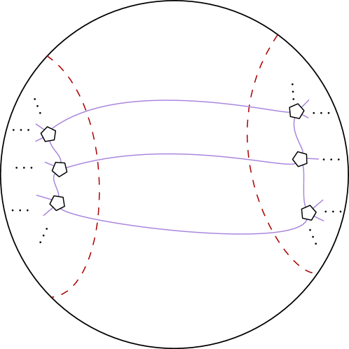
It would be interested to explicitly check the RT surface and bulk reconstruction properties of these networks, especially on fuzzy AdS spaces, perhaps using the methods of Cheng:2022ori ; ffhs:2024xx . In particular, it would be interesting to make sense of tensor network links that might stretch far across the geometry. These modes suggest a natural way to encode mutual information between distant subregions, perhaps inducing backreaction between RT surfaces (see Fig. 19). One could also ask whether the dynamical background independence we consider in this work is identical to the notion of background independence explored in Akers:2024ixq .
It would also be interesting to explore whether such matrix tensor networks are the appropriate language in which to capture (or general higher-derivative) corrections to the entanglement entropy (as in Dong:2013qoa ; Wall:2015raa ). More generally, it is an interesting question whether a matrix tensor network on a fuzzy background (perhaps using the results of Fiore:2022twy ) is the correct way to capture how the compact directions of AdS/CFT may be incorporated into tensor networks. Similarly, it is interesting to check whether these networks accurately capture the ground-state entanglement behavior of BFSS.
Lastly, although we have proposed a manner if incorporating spatial APDs into tensor networks, it is interesting whether time reparameterizations may also be incorporated into such a context, e.g. by using constructions such as Banados:2001xw . Alternatively, it is possible that the dynamics generated by (35) or similar Hamiltonians might be related in some way to bulk time evolution. ffhs:2024xx
Acknowledgements
I am partially supported by the NSF GRFP under grant no. DGE-165-651. I am indebted especially to Xiao-Liang Qi and Aditya Cowsik for extensive insightful discussions. I am also grateful to Ronak M. Soni, Watse Sybesma, Laurens Lootens, Chris Akers, Jason Pollack, and Annie Y. Wei for extensive comments on an early draft. I would like to thank Annie Y. Wei in particular for discussion that inspired the addition of §§3.4. I would also like to thank DAMTP and the University of Cambridge for hospitality during a significant portion of this work.
References
- (1) J.H. Schwarz, Review of recent developments in superstring theory, International Journal of Modern Physics A 2 (1987) 593.
- (2) J. Polchinski, Tasi lectures on d-branes, arXiv preprint hep-th/9611050 (1996) .
- (3) T. Banks, W. Fischler, S.H. Shenker and L. Susskind, M theory as a matrix model: A conjecture, in The World in Eleven Dimensions, pp. 435–451, CRC Press (1999).
- (4) J.M. Maldacena, The Large N limit of superconformal field theories and supergravity, Adv. Theor. Math. Phys. 2 (1998) 231 [hep-th/9711200].
- (5) N. Itzhaki, J.M. Maldacena, J. Sonnenschein and S. Yankielowicz, Supergravity and the large n limit of theories with sixteen supercharges, Physical Review D 58 (1998) 046004.
- (6) D. Berenstein, J. Maldacena and H. Nastase, Strings in flat space and pp waves from super yang mills, Journal of High Energy Physics 2002 (2002) 013.
- (7) S.S. Gubser, I.R. Klebanov and A.M. Polyakov, Gauge theory correlators from non-critical string theory, Physics Letters B 428 (1998) 105.
- (8) E. Witten, Anti de sitter space and holography, arXiv preprint hep-th/9802150 (1998) .
- (9) G. ’t Hooft, A planar diagram theory for strong interactions, in The Large N Expansion In Quantum Field Theory And Statistical Physics: From Spin Systems to 2-Dimensional Gravity, pp. 80–92, World Scientific (1993).
- (10) W. Taylor, M (atrix) theory: Matrix quantum mechanics as a fundamental theory, Reviews of Modern Physics 73 (2001) 419.
- (11) F. Pastawski, B. Yoshida, D. Harlow and J. Preskill, Holographic quantum error-correcting codes: Toy models for the bulk/boundary correspondence, Journal of High Energy Physics 2015 (2015) 1.
- (12) H.R. Hampapura, J. Harper and A. Lawrence, Target space entanglement in Matrix Models, JHEP 10 (2021) 231 [2012.15683].
- (13) P. Hayden, S. Nezami, X.-L. Qi, N. Thomas, M. Walter and Z. Yang, Holographic duality from random tensor networks, JHEP 11 (2016) 009 [1601.01694].
- (14) B. Swingle, Entanglement renormalization and holography, Physical Review D 86 (2012) 065007.
- (15) S. Ryu and T. Takayanagi, Holographic derivation of entanglement entropy from the anti–de sitter space/conformal field theory correspondence, Physical review letters 96 (2006) 181602.
- (16) Z. Yang, P. Hayden and X.-L. Qi, Bidirectional holographic codes and sub-ads locality, Journal of High Energy Physics 2016 (2016) 1.
- (17) R. Sahay, M.D. Lukin and J. Cotler, Emergent Holographic Forces from Tensor Networks and Criticality, 2401.13595.
- (18) C. Akers, R.M. Soni and A.Y. Wei, Multipartite edge modes and tensor networks, 2404.03651.
- (19) X. Dong, S. McBride and W.W. Weng, Holographic tensor networks with bulk gauge symmetries, JHEP 02 (2024) 222 [2309.06436].
- (20) J. Hoppe, Quantum theory of a relativistic surface, in Proceedings of the Workshop “Constraint’s Theory And Relativistic Dynamics”(Florence, 1986), eds. G. Longhi, L. Lusanna (World Scientific, Singapore, 1987), 1982.
- (21) J. Swain, The topology of and the group of area-preserving diffeomorphisms of a compact 2-manifold, Preprint (2004) .
- (22) N. Cheng, C. Lancien, G. Penington, M. Walter and F. Witteveen, Random Tensor Networks with Non-trivial Links, Annales Henri Poincare 25 (2024) 2107 [2206.10482].
- (23) A. Frenkel and S.A. Hartnoll, Entanglement in the Quantum Hall Matrix Model, JHEP 05 (2022) 130 [2111.05967].
- (24) T. Anous and C. Cogburn, Mini-BFSS matrix model in silico, Phys. Rev. D 100 (2019) 066023 [1701.07511].
- (25) X. Han and S.A. Hartnoll, Deep Quantum Geometry of Matrices, Phys. Rev. X 10 (2020) 011069 [1906.08781].
- (26) J. McGreevy, L. Susskind and N. Toumbas, Invasion of the giant gravitons from Anti-de Sitter space, JHEP 06 (2000) 008 [hep-th/0003075].
- (27) X. Dong, Holographic Entanglement Entropy for General Higher Derivative Gravity, JHEP 01 (2014) 044 [1310.5713].
- (28) A.C. Wall, A Second Law for Higher Curvature Gravity, Int. J. Mod. Phys. D 24 (2015) 1544014 [1504.08040].
- (29) J. Polchinski, M theory and the light cone, Prog. Theor. Phys. Suppl. 134 (1999) 158 [hep-th/9903165].
- (30) N. Seiberg and E. Witten, String theory and noncommutative geometry, Journal of High Energy Physics 1999 (1999) 032.
- (31) M.R. Douglas and N.A. Nekrasov, Noncommutative field theory, Reviews of Modern Physics 73 (2001) 977.
- (32) R.J. Szabo, Quantum field theory on noncommutative spaces, Physics Reports 378 (2003) 207.
- (33) E. Witten, Non-commutative geometry and string field theory, Nuclear Physics B 268 (1986) 253.
- (34) F. Ardalan, H. Arfaei and M.M. Sheikh-Jabbari, Noncommutative geometry from strings and branes, JHEP 02 (1999) 016 [hep-th/9810072].
- (35) H. Steinacker, Emergent geometry and gravity from matrix models: an introduction, Classical and Quantum Gravity 27 (2010) 133001.
- (36) H. Steinacker, Non-commutative geometry and matrix models, PoS QGQGS2011 (2011) 004 [1109.5521].
- (37) P.-M. Ho and M. Li, Large n expansion from fuzzy ads2, Nuclear Physics B 590 (2000) 198.
- (38) P.-M. Ho and M. Li, Fuzzy spheres in ads/cft correspondence and holography from noncommutativity, Nuclear Physics B 596 (2001) 259.
- (39) L. Susskind and J. Uglum, Black hole entropy in canonical quantum gravity and superstring theory, Phys. Rev. D 50 (1994) 2700 [hep-th/9401070].
- (40) M. Levin and X.-G. Wen, Detecting topological order in a ground state wave function, Physical review letters 96 (2006) 110405.
- (41) S. Ghosh, R.M. Soni and S.P. Trivedi, On the entanglement entropy for gauge theories, Journal of High Energy Physics 2015 (2015) 1.
- (42) H.R. Hampapura, J. Harper and A. Lawrence, Target space entanglement in matrix models, Journal of High Energy Physics 2021 (2021) 1.
- (43) A. Frenkel and S.A. Hartnoll, Emergent area laws from entangled matrices, Journal of High Energy Physics 2023 (2023) 1.
- (44) J.R. Fliss, A. Frenkel, S.E. Hartnoll and R.M. Soni, Minimal Areas from Entangled Matrices, to appear (2024) .
- (45) S.R. Das, A. Kaushal, G. Mandal and S.P. Trivedi, Bulk entanglement entropy and matrices, Journal of Physics A: Mathematical and Theoretical 53 (2020) 444002.
- (46) S.R. Das, A. Kaushal, G. Mandal and S.P. Trivedi, Bulk Entanglement Entropy and Matrices, J. Phys. A 53 (2020) 444002 [2004.00613].
- (47) J.L. Karczmarek and P. Sabella-Garnier, Entanglement entropy on the fuzzy sphere, Journal of High Energy Physics 2014 (2014) 1.
- (48) L. Susskind, The Quantum Hall fluid and noncommutative Chern-Simons theory, hep-th/0101029.
- (49) S. Hellerman and M. Van Raamsdonk, Quantum Hall physics equals noncommutative field theory, JHEP 10 (2001) 039 [hep-th/0103179].
- (50) A.P. Polychronakos, Quantum Hall states as matrix Chern-Simons theory, JHEP 04 (2001) 011 [hep-th/0103013].
- (51) D. Tong and C. Turner, Quantum Hall effect in supersymmetric Chern-Simons theories, Phys. Rev. B 92 (2015) 235125 [1508.00580].
- (52) W. Zhu, C. Han, E. Huffman, J.S. Hofmann and Y.-C. He, Uncovering Conformal Symmetry in the 3D Ising Transition: State-Operator Correspondence from a Quantum Fuzzy Sphere Regularization, Phys. Rev. X 13 (2023) 021009 [2210.13482].
- (53) A. Tilloy and J.I. Cirac, Continuous Tensor Network States for Quantum Fields, Phys. Rev. X 9 (2019) 021040 [1808.00976].
- (54) J. Madore, The Fuzzy sphere, Class. Quant. Grav. 9 (1992) 69.
- (55) W. Taylor, The M(atrix) model of M theory, NATO Sci. Ser. C 556 (2000) 91 [hep-th/0002016].
- (56) J.E. Moyal, Quantum mechanics as a statistical theory, Proc. Cambridge Phil. Soc. 45 (1949) 99.
- (57) A. Frenkel, Entanglement Edge Modes of General Noncommutative Matrix Backgrounds, 2311.10131.
- (58) C. Akers and A.Y. Wei, Background independent tensor networks, 2402.05910.
- (59) X.-L. Qi, Emergent bulk gauge field in random tensor networks, 2209.02940.
- (60) S. Iso, Y. Kimura, K. Tanaka and K. Wakatsuki, Noncommutative gauge theory on fuzzy sphere from matrix model, Nucl. Phys. B 604 (2001) 121 [hep-th/0101102].
- (61) N. Dorey, D. Tong and C. Turner, Matrix model for non-Abelian quantum Hall states, Phys. Rev. B 94 (2016) 085114 [1603.09688].
- (62) G. Fiore, Fuzzy hyperspheres via confining potentials and energy cutoffs, J. Phys. A 56 (2023) 204002 [2211.13284].
- (63) M. Banados, O. Chandia, N.E. Grandi, F.A. Schaposnik and G.A. Silva, Three-dimensional noncommutative gravity, Phys. Rev. D 64 (2001) 084012 [hep-th/0104264].