Any INFORMS Journal IJDS-0001-1922.65

Forecasting Automotive Supply Chain Disruption with Heterogeneous Time Series

Bach Viet Do

Ford GDIA, 22001 Michigan Ave Dearborn MI 48124 USA, bdo1@ford.com

Xingyu Li

Ford GDIA, 22001 Michigan Ave Dearborn MI 48124 USA, xli236@ford.com

Chaoye Pan

Ford GDIA, 22001 Michigan Ave Dearborn MI 48124 USA, cpan9@ford.com

Oleg Gusikhin Ford GDIA, 22001 Michigan Ave Dearborn MI 48124 USA, ogusikhi@ford.com

Operational disruptions can significantly impact a company’s performance. Ford, with its 37 plants globally, uses 17 billion parts annually to manufacture six million cars and trucks. With up to ten tiers of suppliers between the company and raw materials, any extended disruption in this supply chain can cause substantial financial losses. Therefore, the ability to forecast and identify such disruptions early is crucial for maintaining seamless operations. In this study, we demonstrate how we construct a dataset consisting of many multivariate time series to forecast first-tier supply chain disruptions, utilizing features related to capacity, inventory, utilization, and processing, as outlined in the classical Factory Physics framework. This dataset is technically challenging due to its vast scale of over five hundred thousand time series. Furthermore, these time series, while exhibiting certain similarities, also display heterogeneity within specific subgroups. To address these challenges, we propose a novel methodology that integrates an enhanced Attention Sequence to Sequence Deep Learning architecture, using Neural Network Embeddings to model group effects, with a Survival Analysis model. This model is designed to learn intricate heterogeneous data patterns related to operational disruptions. Our model has demonstrated a strong performance, achieving 0.85 precision and 0.8 recall during the Quality Assurance (QA) phase across Ford’s five North American plants. Additionally, to address the common criticism of Machine Learning models as ”black boxes,” we show how the SHAP framework can be used to generate feature importance from the proposed model’s predictions. It offers valuable insights that can lead to actionable strategies and highlights the potential of advanced machine learning for managing and mitigating supply chain risks in the automotive industry.

Supply Chain Disruption; Supply Chain Resilience; Supply Chain Deep Learning; Survival Analysis; Sequence-to-Sequence

1 Introduction

Ford maintains a complex supply chain and operational network, operating 37 plants globally, utilizing 17 billion parts annually to manufacture six million cars and trucks. The company has up to 10 tiers of suppliers between itself and raw materials. An extended disruption anywhere within this extensive supply chain can inflict a substantial financial impact on the company. In the literature, scholars and practitioners generally agree that disruption negatively impacts the company [31, 12, 26]. However, there is less agreement on classifying and forecasting such disruption [18, 37, 40, 34]. Understanding the different sources and risks of disruption is critical because we can make informed decisions on which disruptions warrant mitigation investment [32]. Supply chain disruptions can stem from many sources, such as global pandemics, natural disasters, geopolitical risks, terrorist attacks, environmental hazards, volatile fuel prices, rising labor costs, currency fluctuations, counterfeit parts and products, delivery delays, market changes, and supplier performance issues.

In the supply chain literature, efforts have been dedicated to modeling the propagation of disruption effects through supply chain networks. One of the early studies by [15] analyzed the propagation of disruption effects through a simplified supply chain. [30] evaluated response strategies to minimize service level impacts in a multi-echelon network during random-duration disruptions. [24] examined the interaction between supplier and buyer response strategies under random-duration disruptions. Simchi-Levi et al. [32, 33] introduced the Time-To-Recover (TTR) metric to quantify the financial impact of disruptions on the entire supply chain, measured by the Risk Exposure Index (REI). This index enables companies to rank their direct and indirect suppliers, identifying the ”weak links” in their supply chains. Additionally, [33] proposed the Time-To-Survive (TTS) concept, which defines the maximum duration the entire supply chain can generally function before the ripple effects of a disruption impact performance. These concepts—TTR, REI, and TTS—have been implemented at Ford Motor Company to manage supply chain risks [33].

These studies are based on the assumption that disruption events can be identified well in advance. In the era of Big Data, the rise of Machine Learning and Artificial Intelligence offers opportunities for predicting disruptive events with high degrees of accuracy. However, the literature on utilizing Machine Learning for supply chain risk management remains sparse. [7] explored the potential of leveraging big data sources related to supply chains and proposed a Supply Chain Risk Management (SCRM) framework to detect emergent risks. [11] recognized the predictive capabilities of incorporating a significant data analytical component into a generic SCRM framework. Nevertheless, these works are theoretical and lack real-world application or implementation of the proposed frameworks and models. More concretely, [42] used a Support Vector Machine classifier to identify disruptions based on the economic performance of firms within the supply chain, collecting public financial data for these firms before, during, and after supply chain disruptions. [2] analyzed historical data from an Original Equipment Manufacturer (OEM) that produced complex engineering assets to predict order delays using machine learning models, including Random Forest, Support Vector Machine, Logistic Regression, and Linear Regression. In their study, the Random Forest Classifier achieved the best performance. Although both studies identify potential suppliers with a high risk of disruptions, they do not provide estimates for the time until these disruption events occur. Such estimates are crucial for integrating this research into the broader framework of Supply Chain Risk Management.

As a leading automobile manufacturer, Ford can request and accumulate an extensive repository of proprietary data on suppliers’ capacity and performance, providing a potent source for highly accurate predictive capabilities. Moreover, Deep Learning has recently emerged as preeminent models in Artificial Intelligence, driven by a decade of rigorous research. Consequently, many state-of-the-art Machine Learning models are now based on Deep Learning.

Our contribution in this work is to advance the research on applying Big Data to forecast supply chain disruptions. We demonstrate the construction of a complex dataset comprising many multivariate time series that track the arrangements between Ford and our first-tier suppliers for transporting critical vehicle parts to Ford’s manufacturing plants. We meticulously select data features that reflect capacity, inventory, utilization, and process time—key aspects in the classical Factory Physics (see [14]). Furthermore, we propose an AI model that integrates an enhanced Sequence to Sequence with Attention Deep Learning architecture with a parametric survival analysis likelihood model. This enhanced architecture is designed to model the heterogeneity in the data, driven by various combinations of plants, sites, and vehicle parts. Our work introduces an important improvement to the Seq2Surv model proposed by [22], developed for generic time series exhibiting similar underlying statistical patterns despite random variations. In contrast, the disruption behaviors in our data can differ markedly, even contradictorily, based on the specific values of suppliers, plants, and parts. While originally developed for supply chain time series data, our methodology can be generalized to any dataset comprising multivariate time series with inherent heterogeneity. Lastly, we illustrate how to use the SHAP (SHapley Additive exPlanations, [27]) framework to calculate feature importance for each of the model’s predictions. This explainable AI technique provides valuable insights that can inform actionable strategies for our business partners.

Our model relies on the Survival Analysis framework to model observed time-to-disruption data. Survival Analysis, a branch of Statistics, focuses on the study of time-to-event data. This field encompasses a variety of applications, such as predicting the survival of cancer patients [39], customer churn [38], mechanical system failure [35], credit scoring [6], and reliability and manufacturing problems [22]. The strength of Survival Analysis lies in its interpretability, flexibility, and ability to handle censored data. However, one of its notable weaknesses is predictive accuracy. To enhance predictive performance, numerous studies have extended classical Survival Analysis using Neural Networks.

[8] were among the pioneers, extending Cox regression by replacing its linear predictor with a single hidden layer multilayer perceptron (MLP). [17] revisited this approach within the deep learning framework, introducing DeepSurv, a model that outperformed traditional Cox models in terms of the C-index (see [10]). Other similar works include SurvivalNet by [43] , which fits Cox proportional models using Neural Networks and applies Bayesian optimization on tuning hyperparameters. [44, 45] utilized Convolutional Neural Networks instead of MLP in their work. [20] proposed an extension of the Cox model where the proportionality constraint is relaxed, introducing an alternative loss function that scales well for both proportional and non-proportional cases. [22] further extended these methodologies by leveraging Sequence-to-Sequence with Attention deep learning architecture for time series survival analysis data.

For discrete-time survival problems, [21] applied neural networks to the discrete-time likelihood for right-censored time-to-event data, parameterizing the probability mass function. [9] adopted a similar likelihood approach, parameterizing hazard rates with a neural network. [19], through simulation studies and real-world data, found that hazard rate parameterization performed slightly better. Building on this insight, the authors introduced PC-Hazard, which parameterization the hazard rate for continuous survival time data by discretizing the continuous time scale, assuming the continuous-time hazard is piece-wise constant.

The remainder of the paper is organized as follows: Section 2 reviews the relevant background and preliminaries. Section 3 offers a detailed explanation of how to construct a dataset for forecasting supply chain disruptions by selecting features that reflect key aspects of classical Factory Physics. In Section 4, we present the Heterogeneous Sequence-to-Disruption AI model. Section 5 evaluates the model’s performance and discusses methods for interpreting the results using the SHAP framework. Finally, Section 6 concludes the paper.

2 Background

2.1 Survival Analysis

In this study, we aim to model the distribution of the time-to-disruption, denoted as $T^{*}$. In practical scenarios, not all disruption times are observable and are often subject to right censoring, wherein the observation period concludes before the disruption event occurs. Let $C^{*}$ represent the time to the censoring event. Formally, we define:

$$T =\min(T^{*},C^{*})$$

$$Y =\mathbbm{1}(T^{*}\leq C^{*}).$$

Here, $T$ is the observed time-to-disruption, and $Y$ is an indicator that equals $1$ if the disruption event occurs within the observation window $T^{*}\leq C^{*}$ and $0$ otherwise. This framework is fundamental in Survival Analysis, a branch of statistics focusing on time-to-event data [16]. As demonstrated in the next section, in our data, the time-to-disruption is discrete, ranging from $1$ to $365$ days. The discrete disruption time can be modeled using a parametric approach (see Chapter 10 in [25]).

Before we define the model, let’s go over some preliminaries. Consider a random discrete variable $T^{*}$ with the discrete support $\tau_{1}<\tau_{2}<\ldots<\tau_{j}<\ldots$, the cumulative distribution function (CDF) is given by $F(t)=P(T^{*}\leq t)=\sum_{i=0}^{t}\mathbb{P}(T^{*}=t)$, and the corresponding probability mass function (PMF) is $f(t)=\mathbb{P}(T^{*}=t)$.

In Survival Analysis, it’s often more useful to discuss the survival function, defined as $S(t)=1-F(t)=P(T^{*}>t)$, along with its associated hazard function. For a discrete variable $T^{*}$ and two consecutive survival time points $\tau_{j-1}<\tau_{j}$, the hazard function is denoted $h(\tau_{j})=\mathbb{P}(T^{*}=\tau_{j}\;|\;T^{*}>\tau_{j-1})=\cfrac{f(\tau_{j})}{S(\tau_{j-1})}=\cfrac{S(\tau_{j-1})-S(\tau_{j})}{S(\tau_{j-1})}$. As such,

$$f(\tau_{j})=h(\tau_{j})S(\tau_{j-1})$$ (1)

$$S(\tau_{j})=[1-h(\tau_{j})]S(\tau_{j-1}).$$ (2)

On the other hand, we see that,

$$\mathbb{P}(T=t,Y=y) =\mathbb{P}(T=t,t\leq C^{*})^{y}\mathbb{P}(T=t,t>C^{*})^{1-y}$$

$$=f(t)^{y}\mathbb{P}(C^{*}\geq t)^{y}\mathbb{P}(T^{*}>t,C^{*}=t)^{1-y}$$

$$=f(t)^{y}\mathbb{P}(C^{*}\geq t)^{y}\mathbb{P}(T^{*}>t)^{1-y}\mathbb{P}(C^{*}=t)^{1-y}$$

$$=f(t)^{y}S(t)^{1-y}\mathbb{P}(C^{*}\geq t)^{y}\mathbb{P}(C^{*}=t)^{1-y}.$$

The third equality is due to $T^{*}$ and $C^{*}$ are independent. Since random variable $T$ is discrete, we can model the hazard function using a parametric distribution with parameter $\theta$. We define $\kappa(t)$ as the index of the discrete time point in the support, i.e., $t=\tau_{\kappa(t)}$. For a sample of observations $(t_{1},y_{1}),(t_{2},y_{2}),\ldots,(t_{n},y_{n})$, the log-likelihood function can be expressed as a sum of individual log-likelihood contributions as follows using equations (1) and (2).

$$l(\theta) =\sum_{i=1}^{n}y_{i}\log f_{\theta}(t_{i})+\sum_{i=1}^{n}(1-y_{i})\log S_{\theta}(t_{i})+\sum_{i=1}^{n}\left[y_{i}\log P(C^{*}_{i}\geq t_{i})+(1-y_{i})\log\mathbb{P}(C^{*}_{i}=t_{i})\right]$$

$$\propto\sum_{i=1}^{n}y_{i}\log f_{\theta}(t_{i})+\sum_{i=1}^{n}(1-y_{i})\log S_{\theta}(t_{i})$$

$$=\sum_{i=1}^{n}y_{i}\log h_{\theta}(t_{i})+y_{i}\log S(\tau_{\kappa(t_{i})-1})+\sum_{i=1}^{n}(1-y_{i})\log[1-h_{\theta}(t_{i})]+(1-y_{i})\log S_{\theta}(\tau_{\kappa(t_{i})-1})$$

$$=\sum_{i=1}^{n}\left[y_{i}\log h_{\theta}(t_{i})+(1-y_{i})\log[1-h_{\theta}(t_{i})]+S(t_{\kappa(t_{i})-1})\right].$$

In the second equality, terms related to censoring times $C_{i}$ are omitted from the log-likelihood function as they are constant and do not contain parameter $\theta$. Utilizing equation 2 recursively in the final term of the last equality above, we can finally write the log-likelihood of the sample data as,

$$l(\theta)=\sum_{i=1}^{n}\left[y_{i}\log h_{\theta}(t_{i})+(1-y_{i})\log[1-h_{\theta}(t_{i})]+\sum_{j=1}^{\kappa(t_{i})-1}\log[1-h_{\theta}(\tau_{j})]\right].$$ (3)

Observe that the equation 3 consists solely of the hazard function. To model the observed data, we simply need to define the form of the hazard function. Since the hazard function represents a probability in discrete form, its range must lie between 0 and 1. One suitable choice is the logistic hazard function (see [3]). Assume that the time-to-disruption is also conditioned on covariates/features $X$,

$$h(\tau_{k})=\cfrac{1}{1+\exp\left(-\theta_{k}^{T}X\right)},k=1,2,\ldots,$$ (4)

where $\theta$ is the model parameter and the linear combination $\theta^{T}X$ reflects the linear relationship between the features and the model parameter.

2.2 Sequence-to-Sequence Architecture

The Seq2Seq model, introduced by [36] at Google, represents a pivotal milestone in deep learning. This model processes a sequence of inputs to generate a corresponding sequence of outputs. While initially developed to address the challenges of machine translation, the Seq2Seq model has since become a foundational framework for various natural language processing tasks and has been adopted for time series data in other fields.

The core architecture of the Seq2Seq model is the encoder-decoder framework, which is frequently implemented using Recurrent Neural Networks (RNNs, see [29]). The encoder’s primary function is to convert the sequential input data into hidden states and a context vector. The context vector, the aggregated sum of these hidden states, encapsulates the information from the input sequence into a fixed-size representation.

Once the input sequence has been encoded, the decoder generates the output sequence. It leverages the context vector and hidden states to produce the output sequence. Operating in an autoregressive manner, the decoder generates one unit of the output sequence at a time. This step-by-step generation ensures that each subsequent unit is conditioned on the previously generated units, thereby maintaining coherence in the output sequence.

A significant enhancement to the Seq2Seq model is integrating the Attention mechanism proposed by [1]. This mechanism enables the model to dynamically focus on different parts of the input sequence while generating each output unit. Specifically, the context vector is computed as a weighted sum of the encoder’s hidden states, with the weights reflecting the relevance of each hidden state to the current decoding step. This dynamic focusing capability significantly improves the model’s performance, particularly for tasks involving long and complex input sequences.

2.3 Seq2Surv Model

Leveraging the power of Sequence-to-Sequence neural networks and the Attention mechanism for modeling sequential data, [22] employs this advanced deep learning architecture to handle time series data in the reliability and manufacturing domain. This approach replaces the linear predictor in Cox proportional hazard models (see Chapter 5 in [25]) and discrete time logistic hazard parametric models (see equation 4) with learnable non-linear functions. In this methodology, time series are treated as sequential input to the Encoder, which [22] implemented using Bidirectional Gated Recurrent Units (GRUs), as introduced by [5]. The GRU, similar to a Long Short-Term Memory network (LSTM, see [13]) with its gating mechanisms for input and forgetting features, lacks output gates, resulting in fewer parameters than LSTMs. The Decoder in Seq2Surv then generates a sequence of survival probability estimates for the entire lifetime, which is then used in the Survival Analysis’ log-likelihood function to model the observed disruption times.

3 Model Performance & Explainability

3.1 Predictive Performance

Ford Plant	Precision	Recall	Normalized Confusion Matrix
			True Positive	False Negative	False Positive	True Negative
Kansas City Assembly Plant	0.85	0.82	0.23	0.05	0.04	0.68
Michigan Assembly Plant	0.95	0.9	0.22	0.02	0.00	0.75
Dearborn Truck Plant	0.95	0.81	0.15	0.04	0.01	0.8
Ohio Assembly Plant	0.95	0.86	0.21	0.03	0.01	0.75
Kentucky Truck Plant	0.85	0.81	0.25	0.06	0.04	065

Table 1: Quality Assurance (QA) performance of the model for five selected plants in North America. Metrics were calculated using the definitions of Adapted True Positive, False Negative, False Positive, and True Negative as previously described. For brevity, ’Adapted’ is omitted in the column names.

In this section, we detail the approach for evaluating the proposed model at Ford to ensure its quality. The trained model estimates the time until a disruption event occurs related to the shipment of vehicle parts between a supplier and a Ford plant. To assess the model’s performance, we modify and adapt the standard classification metrics to fit our specific needs.

In binary classification, the two standard metrics for evaluation are Precision and Recall (see [4]). Binary classification involves two labels: positive and negative. For a given classifier, True Positives (TP) are the instances where the classifier correctly identifies positives. True Negatives (TN) are the instances where the classifier correctly identifies negatives. False Positives are instances where the classifier incorrectly predicts positives when the true label is negative. Conversely, False Negatives (FN) are instances where the classifier incorrectly predicts negatives when the true label is positive. Formally, Precision and Recall are defined as,

$$\text{Precision}=\cfrac{\text{TP}}{\text{TP}+\text{FP}}$$

$$\text{Recall}=\cfrac{\text{TP}}{\text{TP}+\text{FN}}.$$

Precision and recall range from $0$ to $1$. The closer these values are to $1$, the better the classifier’s performance. Specifically, recall quantifies the proportion of actual positive data points that the classifier successfully identifies. Precision, on the other hand, measures the proportion of predicted positive cases that are, in fact, positive. Informally, recall measures how effectively a classifier identifies positive events (disruptions in this context), while precision measures the frequency with which the classifier avoids generating false alarms. These two metrics offer a comprehensive view of a model’s classification performance.

Given that the model proposed in Section LABEL:model estimates the time until a disruption, we first define a forecasting horizon, $\Delta$ (in days), and a margin-of-error, $\epsilon$ (in days), to evaluate its performance. We introduce the following definitions to adapt the concepts of True Positives, False Positives, True Negatives, and False Negatives to our specific problem. Given an observation time $t_{0}$, and the forecasting window $\Delta$ and margin-of-error $\epsilon$, $t_{0}+\Delta$ represents a time point $\Delta$ days from $t_{0}$. Adapted True Positives (ATP) are defined as the number of disruptions that occur exactly $\Delta$ days from $t_{0}$ and are estimated by the model within $\epsilon$ days of $t_{0}+\Delta$. The difference between the model’s estimated time and $t_{0}+\Delta$ must fall within the range $[-\epsilon,\epsilon]$ days. Adapted False Positives (AFP) are instances where the model predicts a disruption time exactly $\Delta$ days from $t_{0}$, but no disruptions actually occur within $\epsilon$ days of $t_{0}+\Delta$.

Conversely, Adapted True Negatives (ATN) are instances where the model estimates the disruption time to be more than $\Delta$ days from $t_{0}$, and no disruptions occur between $t_{0}$ and $t_{0}+\Delta$. Adapted False Negatives (AFN) are instances where the model predicts a disruption time beyond $\Delta$ from $t_{0}$, while disruptions actually occur within $\Delta$ days from $t_{0}$.

With these definitions, Adapted Recall is computed as the ratio of Adapted True Positives (ATP) to the total of ATP and Adapted False Negatives (AFN). Likewise, Adapted Precision is the proportion of ATP relative to the sum of ATP and Adapted False Positives (AFP). Additionally, we provide the Normalized Confusion Matrix in Table 1 also known as the error matrix. This table offers a detailed visualization of the four cases: True Positives, False Negatives, False Positives, and True Negatives. The normalization is done by dividing each case by the total number of cases.

Model on Data	Performance Metrics
	Precision	Recall
Seq2Surv on Kansas Assembly Plant Data	0.62	0.3
Seq2Surv on Kentucky Truck Plant	0.52	0.21
Heterogeneous Seq2Surv on Kansas Assembly Plant Data	0.85	0.82
Heterogeneous Seq2Surv on Kentucky Truck Plant	0.85	0.81

Table 2: Model Performance Comparison of Seq2Surv and Heterogeneous Seq2Surv on Kansas Assembly Plant and Kentucky Truck Plant Datasets. Heterogeneity presents a critical challenge for Seq2Surv.

We conducted 20 iterations of Quality Assurance (QA) testing from August 1, 2023, to January 13, 2024 for the result in Table 1. For each observation week, we trained the model on the cumulative data up to that week and used it to predict disruptions in the near future. We computed Adapted Precision, Adapted Recall, and the Normalized Confusion Matrix using definitions for Adapted True Positives, True Negatives, False Positives, and False Negatives, with parameters forecasting horizon $\Delta=28$ days and margin-of-error $\epsilon=7$ days. The metrics in Table 1 are averaged over the 20 iterations. The Quality Assurance (QA) evaluation was conducted at five selected Ford manufacturing facilities in North America: Kansas City Assembly Plant, Michigan Assembly Plant, Dearborn Truck Plant, Ohio Assembly Plant, and Kentucky Truck Plant.

The model demonstrated on average precision exceeding $0.85$ and a recall surpassing $0.8$ across the five plants during the 20-week QA period. Additionally, the normalized confusion matrix indicates that the combined error rate of false positive and false negative errors was below $10$% on average. Furthermore, we present performance comparison between Seq2Surv, as described in [22], and our Heterogeneous Seq2Surv proposed in Section LABEL:model, as shown in Table 2. The metrics provided are the averages obtained from 20 iterations of QA testing. Our analysis reveals that the heterogeneity in plant, supplier, and part groups poses significant challenges for Seq2Surv. However, by incorporating heterogeneous behaviors in the data into the model, our Heterogeneous Seq2Surv demonstrates substantially improved performance. For a comparison between Seq2Surv and other models, please refer to [22].

3.2 Explainable AI with SHAP

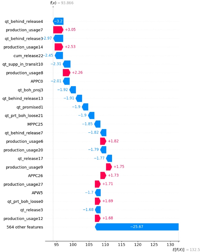
Figure 1: Utilizing the SHAP (SHapley Additive exPlanations) framework to calculate feature importance for a specific prediction instance made by the trained model.

The proposed model demonstrates desirable predictive performance, largely due to the Sequence-to-Sequence Neural Network’s capability to capture complex non-linear relationships. However, despite their effectiveness, Deep Learning models often face criticism for their ”black-box” nature. The complexity of these models frequently makes it difficult to understand their underlying mechanisms or interpret internal embeddings and representations (see [41]). This lack of transparency is a significant challenge in a multi-departmental corporation like Ford, where it is essential to adequately communicate the model’s behaviors and decision-making processes to provide actionable insights to the Business department.

Explainable Artificial Intelligence (XAI) is an emerging field dedicated to developing principles, frameworks, and tools to elucidate the reasoning behind AI decisions and predictions (see [27]). A prominent technique in this area is the Shapley value, which is based on cooperative game theory (see [23]).

Introduced by Lloyd Shapley in 1951, the Shapley value is a technique for fairly allocating profits among players in a cooperative game, adhering to four fairness axioms (see [28]). In machine learning, Shapley values can be applied by treating features as players and the model’s behavior as the profit. This approach allows us to quantify the impact of each feature. The SHAP (SHapley Additive exPlanations) framework, popularized by [23], utilizes Shapley values to explain individual predictions. Figure 1 demonstrates the application of the SHAP framework to a specific prediction instance using the model described in Section LABEL:model. The waterfall plot illustrates the important factors influencing the model’s predicted time-to-disruption, such as the progression of ‘’qt_behind_release‘’ over 13, 7, 4, and 3 days ago, and the progression of ‘’production_usage‘’ over 27, 14, 12, 9, 8, 7, and 6 days ago, among others. This information enables a deeper investigation into the data, helping to uncover the potential reasons behind the model’s prediction for this specific instance.

4 Conclusion

In this paper, we first outline the process of constructing a dataset of multivariate time series for forecasting first-tier supply chain disruptions. We carefully selected features representing key aspects of classical Factory Physics, such as capacity, inventory, utilization, and processing.

The dataset, comprising over five hundred thousand individual time series, presents significant technical challenges due to its complexity and scale. Although these time series exhibit some commonalities, they also demonstrate substantial heterogeneity within specific subgroups, making traditional industrial and statistical models inadequate for capturing the intricate dynamics and managing the extensive data volume. To address these challenges, we propose a novel methodology that integrates an enhanced Attention Sequence-to-Sequence Deep Learning architecture with Neural Network Embeddings to model group effects, combined with a Survival Analysis model. This approach is designed to effectively capture complex heterogeneous data patterns related to operational disruptions. Our model has achieved strong performance, with at least $85$% precision and $80$% recall during the Quality Assurance (QA) phase across Ford’s five North American plants.

To mitigate the common critique of Machine Learning models as ”black boxes,” we employed the SHAP (SHapley Additive exPlanations) framework to elucidate feature importance in the model’s predictions. This technique provides valuable insights that can guide actionable strategies for business partners. Our work highlights the potential of advanced machine learning techniques to manage and mitigate supply chain risks effectively within the automotive industry.

References

- [1] Dzmitry Bahdanau, Kyunghyun Cho and Yoshua Bengio “Neural machine translation by jointly learning to align and translate” In arXiv preprint arXiv:1409.0473, 2014
- [2] Alexandra Brintrup, Johnson Pak, David Ratiney, Tim Pearce, Pascal Wichmann, Philip Woodall and Duncan McFarlane “Supply chain data analytics for predicting supplier disruptions: a case study in complex asset manufacturing” In International Journal of Production Research 58.11 Taylor & Francis, 2020, pp. 3330–3341
- [3] Charles C Brown “On the use of indicator variables for studying the time-dependence of parameters in a response-time model” In Biometrics JSTOR, 1975, pp. 863–872
- [4] Michael Buckland and Fredric Gey “The relationship between recall and precision” In Journal of the American society for information science 45.1 Wiley Online Library, 1994, pp. 12–19
- [5] Kyunghyun Cho, Bart Van Merriënboer, Dzmitry Bahdanau and Yoshua Bengio “On the properties of neural machine translation: Encoder-decoder approaches” In arXiv preprint arXiv:1409.1259, 2014
- [6] Lore Dirick, Gerda Claeskens and Bart Baesens “Time to default in credit scoring using survival analysis: a benchmark study” In Journal of the Operational Research Society 68.6 Taylor & Francis, 2017, pp. 652–665
- [7] Yingjie Fan, Leonard Heilig and Stefan Voß “Supply chain risk management in the era of big data” In Design, User Experience, and Usability: Design Discourse: 4th International Conference, DUXU 2015, Held as Part of HCI International 2015, Los Angeles, CA, USA, August 2–7, 2015, Proceedings, Part I, 2015, pp. 283–294 Springer
- [8] David Faraggi and Richard Simon “A neural network model for survival data” In Statistics in medicine 14.1 Wiley Online Library, 1995, pp. 73–82
- [9] Michael F Gensheimer and Balasubramanian Narasimhan “A scalable discrete-time survival model for neural networks” In PeerJ 7 PeerJ Inc., 2019, pp. e6257
- [10] Frank E Harrell, Robert M Califf, David B Pryor, Kerry L Lee and Robert A Rosati “Evaluating the yield of medical tests” In Jama 247.18 American Medical Association, 1982, pp. 2543–2546
- [11] Longfei He, Mei Xue and Bin Gu “Internet-of-things enabled supply chain planning and coordination with big data services: Certain theoretic implications” In Journal of Management Science and Engineering 5.1 Elsevier, 2020, pp. 1–22
- [12] Kevin B Hendricks and Vinod R Singhal “Association between supply chain glitches and operating performance” In Management science 51.5 INFORMS, 2005, pp. 695–711
- [13] Sepp Hochreiter and Jürgen Schmidhuber “Long short-term memory” In Neural computation 9.8 MIT press, 1997, pp. 1735–1780
- [14] Wallace J Hopp and Mark L Spearman “Factory physics” Waveland Press, 2011
- [15] Wallace J Hopp and Zigeng Yin “Protecting supply chain networks against catastrophic failures” In not yet published, 2006
- [16] Stephen P Jenkins “Survival analysis” In Unpublished manuscript, Institute for Social and Economic Research, University of Essex, Colchester, UK 42 Citeseer, 2005, pp. 54–56
- [17] Jared L Katzman, Uri Shaham, Alexander Cloninger, Jonathan Bates, Tingting Jiang and Yuval Kluger “DeepSurv: personalized treatment recommender system using a Cox proportional hazards deep neural network” In BMC medical research methodology 18 Springer, 2018, pp. 1–12
- [18] Paul R Kleindorfer and Germaine H Saad “Managing disruption risks in supply chains” In Production and operations management 14.1 SAGE Publications Sage CA: Los Angeles, CA, 2005, pp. 53–68
- [19] Håvard Kvamme and Ørnulf Borgan “Continuous and discrete-time survival prediction with neural networks” In arXiv preprint arXiv:1910.06724, 2019
- [20] Håvard Kvamme, Ørnulf Borgan and Ida Scheel “Time-to-event prediction with neural networks and Cox regression” In Journal of machine learning research 20.129, 2019, pp. 1–30
- [21] Changhee Lee, William Zame, Jinsung Yoon and Mihaela Van Der Schaar “Deephit: A deep learning approach to survival analysis with competing risks” In Proceedings of the AAAI conference on artificial intelligence 32.1, 2018
- [22] Xingyu Li, Vasiliy Krivtsov and Karunesh Arora “Attention-based deep survival model for time series data” In Reliability Engineering & System Safety 217 Elsevier, 2022, pp. 108033
- [23] Scott M Lundberg and Su-In Lee “A unified approach to interpreting model predictions” In Advances in neural information processing systems 30, 2017
- [24] Cameron A MacKenzie, Kash Barker and Joost R Santos “Modeling a severe supply chain disruption and post-disaster decision making with application to the Japanese earthquake and tsunami” In IIE Transactions 46.12 Taylor & Francis, 2014, pp. 1243–1260
- [25] Dirk F Moore “Applied survival analysis using R” Springer, 2016
- [26] Risk Response Network “Building resilience in supply chains”, 2013 Technical report, The World Economic Forum
- [27] P Jonathon Phillips, P Jonathon Phillips, Carina A Hahn, Peter C Fontana, Amy N Yates, Kristen Greene, David A Broniatowski and Mark A Przybocki “Four principles of explainable artificial intelligence” US Department of Commerce, National Institute of StandardsTechnology, 2021
- [28] Alvin E Roth “The Shapley value: essays in honor of Lloyd S. Shapley” Cambridge University Press, 1988
- [29] David E Rumelhart, Geoffrey E Hinton and Ronald J Williams “Learning internal representations by error propagation, parallel distributed processing, explorations in the microstructure of cognition, ed. de rumelhart and j. mcclelland. vol. 1. 1986” In Biometrika 71.599-607, 1986, pp. 6
- [30] Amanda J Schmitt “Strategies for customer service level protection under multi-echelon supply chain disruption risk” In Transportation Research Part B: Methodological 45.8 Elsevier, 2011, pp. 1266–1283
- [31] Yossi Sheffi “The resilient enterprise: overcoming vulnerability for competitive advantage” Pearson Education India, 2005
- [32] David Simchi-Levi, William Schmidt and Yehua Wei “From superstorms to factory fires: Managing unpredictable supply chain disruptions” In Harvard Business Review 92.1-2, 2014, pp. 96–101
- [33] David Simchi-Levi, William Schmidt, Yehua Wei, Peter Yun Zhang, Keith Combs, Yao Ge, Oleg Gusikhin, Michael Sanders and Don Zhang “Identifying risks and mitigating disruptions in the automotive supply chain” In Interfaces 45.5 INFORMS, 2015, pp. 375–390
- [34] ManMohan S Sodhi, Byung-Gak Son and Christopher S Tang “Researchers’ perspectives on supply chain risk management” In Production and operations management 21.1 SAGE Publications Sage CA: Los Angeles, CA, 2012, pp. 1–13
- [35] Gian Antonio Susto, Andrea Schirru, Simone Pampuri, Seán McLoone and Alessandro Beghi “Machine learning for predictive maintenance: A multiple classifier approach” In IEEE transactions on industrial informatics 11.3 IEEE, 2014, pp. 812–820
- [36] Ilya Sutskever, Oriol Vinyals and Quoc V Le “Sequence to sequence learning with neural networks” In Advances in neural information processing systems 27, 2014
- [37] Christopher S Tang “Robust strategies for mitigating supply chain disruptions” In International Journal of Logistics: Research and Applications 9.1 Taylor & Francis, 2006, pp. 33–45
- [38] Dirk Van den Poel and Bart Lariviere “Customer attrition analysis for financial services using proportional hazard models” In European journal of operational research 157.1 Elsevier, 2004, pp. 196–217
- [39] Antonio Viganò, Marlene Dorgan, Jeanette Buckingham, Eduardo Bruera and Maria E Suarez-Almazor “Survival prediction in terminal cancer patients: a systematic review of the medical literature” In Palliative Medicine 14.5 Sage Publications Sage CA: Thousand Oaks, CA, 2000, pp. 363–374
- [40] Stephan M Wagner and Christoph Bode “An empirical investigation into supply chain vulnerability” In Journal of purchasing and supply management 12.6 Elsevier, 2006, pp. 301–312
- [41] Jinjiang Wang, Yulin Ma, Laibin Zhang, Robert X Gao and Dazhong Wu “Deep learning for smart manufacturing: Methods and applications” In Journal of manufacturing systems 48 Elsevier, 2018, pp. 144–156
- [42] ShiJie Ye, Zhi Xiao and Guangfu Zhu “Identification of supply chain disruptions with economic performance of firms using multi-category support vector machines” In International Journal of Production Research 53.10 Taylor & Francis, 2015, pp. 3086–3103
- [43] Safoora Yousefi et al. “Predicting clinical outcomes from large scale cancer genomic profiles with deep survival models” In Scientific reports 7.1 Nature Publishing Group, 2017, pp. 1–11
- [44] Xinliang Zhu, Jiawen Yao and Junzhou Huang “Deep convolutional neural network for survival analysis with pathological images” In 2016 IEEE international conference on bioinformatics and biomedicine (BIBM), 2016, pp. 544–547 IEEE
- [45] Xinliang Zhu, Jiawen Yao, Feiyun Zhu and Junzhou Huang “Wsisa: Making survival prediction from whole slide histopathological images” In Proceedings of the IEEE conference on computer vision and pattern recognition, 2017, pp. 7234–7242