Abstract

In this article, we focus on solving a class of distributed optimization problems involving $n$ agents with the local objective function at every agent $i$ given by the difference of two convex functions $f_{i}$ and $g_{i}$ (difference-of-convex (DC) form), where $f_{i}$ and $g_{i}$ are potentially nonsmooth. The agents communicate via a directed graph containing $n$ nodes. We create smooth approximations of the functions $f_{i}$ and $g_{i}$ and develop a distributed algorithm utilizing the gradients of the smooth surrogates and a finite-time approximate consensus protocol. We term this algorithm as DDC-Consensus. The developed DDC-Consensus algorithm allows for non-symmetric directed graph topologies and can be synthesized distributively. We establish that the DDC-Consensus algorithm converges to a stationary point of the nonconvex distributed optimization problem. The performance of the DDC-Consensus algorithm is evaluated via a simulation study to solve a nonconvex DC-regularized distributed least squares problem. The numerical results corroborate the efficacy of the proposed algorithm.
keywords: Distributed optimization, nonconvex optimization, difference-of-convex (DC) functions, DC programming, distributed gradient descent, directed graphs.

Distributed Difference of Convex Optimization

Vivek Khatana, Murti V. Salapaka Vivek Khatana (Email: {khata010}@umn.edu) and Murti V. Salapaka (Email: {murtis}@umn.edu) are with the Department of Electrical and Computer Engineering, University of Minnesota, Minneapolis, USA.

I Introduction

Due to the increase in size and complexity of modern systems, solving problems involving many agents via distributed methods is highly desirable. An effective way towards a distributed solution is to cast the problems in the framework of distributed optimization [1, 2]. In this article, we focus on the following distributed optimization problem,

$\displaystyle\textstyle\operatorname*{minimize}\limits_{x\in\mathbb{R}^{p}}\ F(x)=\frac{1}{n}\sum_{i=1}^{n}(f_{i}(x)-g_{i}(x)),$ (1)

where $x\in\mathbb{R}^{p}$ is a common decision, and $f_{i}:\mathbb{R}^{p}\to\mathbb{R}\cup\{-\infty,\infty\}$ and $g_{i}:\mathbb{R}^{p}\to\mathbb{R}$ are private objective functions of agent $i$. The agents are connected through a directed graph, $\mathcal{G}(\mathcal{V},\mathcal{E})$, where $\mathcal{V}$ and $\mathcal{E}$ are the set of vertices and edges respectively. The terms in the aggregate objective function in (1) are of a difference-of-convex (DC) form. Due to the richness of the set of DC functions (see the properties mentioned in [3]), DC functions can be used to model most of all practical non-convex optimization problems. Many applications in statistical learning and estimation [4], power systems [5], computational biology [6], signal restoration [7], network optimization [8], combinatorial optimization [9] can be posed as DC programs.

The initial study of distributed optimization can be traced back to the seminal works [10, 11]. Since then the special case with $f_{i}$ being convex and $g_{i}=0$ has received significant development (see [12, 13, 14] and references therein). As a relaxation of the convex objective functions most works in the literature are restricted to Lipschitz differentiable not necessarily convex functions $f_{i}$ with $g_{i}=0$ (some examples include [15, 16, 17, 18, 19, 20, 21]) and do not address the general problem (1). Article [22] focuses on a special case with weakly convex objective functions $f_{i}$ and $g_{i}=0$. Article [23] considers a DC form however the functions $f_{i}$ and $g_{i}$ are assumed to have Lipschitz differentiable gradients, and does not ensure globally agreed decisions among all the agents. To the best of the authors’ knowledge, the general distributed optimization problem (1) with DC functions is not addressed in prior works.

However, DC programming is studied in the centralized optimization literature [24, 25, 26, 27, 28, 29, 30]. Articles [24, 25, 26, 27, 28] utilize an affine minorization $g_{i}^{m}$ of the functions $g_{i},i=1$ and minimize the resulting convex function $f_{i}-g_{i}^{m},i=1$. The work in [29] provides an accelerated version of the algorithms proposed in [24, 25, 26, 27, 28] using adaptive step-sizes and extrapolation of the algorithm iterates. Article [30] proposed an alternating direction of multipliers method based algorithm for solving centralized DC optimization problems with Lipschitz differentiable functions and a linear equality constraint. The current article is closest to the centralized algorithms [31, 32], where a majorization of the objective functions via the proximal mapping is solved.

In this article, we propose an iterative algorithm termed Distributed DC-Consensus DDC-Consensus. The DDC-Consensus algorithm proceeds in two steps: first, all the agents in parallel solve a local optimization problem involving $f_{i}-g_{i}$, then each agent $i\in\mathcal{V}$ shares the obtained solution with its neighbors where the estimates of the global solution are updated by utilizing an average consensus protocol (the algorithm is presented in detail in Section II-B). The main contributions of the current article are as follows:
i) We develop a distributed algorithm, DDC-Consensus, based on distributed gradient descent to the solve (1) for non-differentiable weakly convex $f_{i}$ and non-differentiable convex function $g_{i}$. These assumptions are weaker than the existing literature on distributed optimization.
ii) We establish that the DDC-Consensus converges to a stationary solution of the nonconvex problem (1).
iii) The proposed DDC-Consensus algorithm has desirable properties as it (a) is suitable for directed graphs and non-symmetric communication topologies, and (b) can be implemented as well as synthesized distributively.
We demonstrate the performance of the DDC-Consensus algorithm by solving a DC-regularized least squares problem. Empirical results from the numerical simulation study corroborate that the proposed DDC-Consensus algorithm performs well in practice.

The rest of the article is organized as follows: Some essential definitions and notations are presented in Section I-A. Section II provides the details of the proposed DDC-Consensus algorithm. Convergence analysis of DDC-Consensus is presented in Section III. Section IV presents the numerical simulation study followed by concluding remarks in Section V.

I-A Definitions and Notations

Definition 1.

(Directed Graph) A directed graph $\mathcal{G}$ is a pair $(\mathcal{V},\mathcal{E})$ where $\mathcal{V}$ is a set of vertices and $\mathcal{E}$ is a set of edges, which are ordered subsets of two distinct elements of $\mathcal{V}$. If an edge from $j\in\mathcal{V}$ to $i\in\mathcal{V}$ exists it is denoted as $(i,j)\in\mathcal{E}$.

Definition 2.

(Strongly Connected Graph) A directed graph is strongly connected if for any pair $(i,j),\ i\not=j$, there is a directed path from node $i$ to node $j$.

Definition 3.

(Diameter of a Graph) The longest shortest directed path between any two nodes in the graph.

Definition 4.

(In-Neighborhood) The set of in-neighbors of node $i\in\mathcal{V}$ is called the in-neighborhood of node $i$ and is denoted by $\mathcal{N}^{-}_{i}=\{j\ |\ (i,j)\in\mathcal{E}\}$ not including the node $i$.

Definition 5.

(Column-Stochastic Matrix) A matrix $M=[m_{ij}]\in\mathbb{R}^{n\times n}$ is called a column-stochastic matrix if $0\leq m_{ij}\leq 1$ and $\sum_{i=1}^{n}m_{ij}=1$ for all $1\leq i,j\leq n$.

Definition 6.

(Lipschitz Continuity and Differentiability) A function $f:\mathbb{R}^{p}\to\mathbb{R}$ is called Lipschitz continuous with constant $L>0$ and Lipschitz differentiable with constant $L_{f}>0$ respectively, if the following inequalities hold:

$\displaystyle|f(x)-f(y)|$ $\displaystyle\leq L\|x-y\|,\ \forall\ x,y\in\mathbb{R}^{p}$
$\displaystyle\|\nabla f(x)-\nabla f(y)\|$ $\displaystyle\leq L_{f}\|x-y\|,\ \forall\ x,y\in\mathbb{R}^{p}.$
Definition 7.

(Strongly Convex Function) A differentiable function $f$ is called strongly convex with parameter $\sigma$, if there exists $\sigma>0$ such that for all $x,y$ in the domain of $f$:

$\displaystyle\langle\nabla f(x)-\nabla f(y),x-y\rangle\geq\sigma\|x-y\|^{2},\ \forall\ x,y\in\operatorname*{dom}f.$
Definition 8.

(Weakly Convex Function) For some $m_{f}\geq 0$, we say that function $f:\mathbb{R}^{p}\to\mathbb{R}$ is $m_{f}$-weakly convex if $f+\frac{m_{f}}{2}\|x\|^{2}$ is convex.

Definition 9.

(Level-bounded Function) Function $f:\mathbb{R}^{p}\to\mathbb{R}$ is called level-bounded if the $\beta$-level-set $\{x:f(x)\leq\beta\}$ is bounded (possibly empty) for all $\beta\in\mathbb{R}$.

Definition 10.

(Lower Semicontinuity) A function $f:\mathbb{R}^{p}\to\mathbb{R}\cup\{-\infty,\infty\}$ is called lower semi-continuous at a point $x_{0}$ if for every real $y<f(x_{0})$ there exists a neighborhood $U$ of $x_{0}$ such that $y<f(x)$ for all $x\in U$. The function $f$ is lower semicontinuous at every point of its domain, $\operatorname*{dom}(f)$.

Definition 11.

(Proper Function) A function $f:\mathbb{R}^{p}\to\mathbb{R}\cup\{-\infty,\infty\}$ is called proper if $f(x)>-\infty$ for every $x$ and and if there also exists some point $x_{0}$ such that $f(x_{0})<\infty$.

$\|x\|_{1}$ and $\|x\|$ denote the 1-norm and 2-norm of the vector $x\in\mathbb{R}^{p}$ respectively. The notation $\left\lceil.\right\rceil$ denotes the least integer function or the ceiling function, defined as: given $x\in\mathbb{R},\left\lceil x\right\rceil=\min\{m\in\mathbb{Z}|m\geq x\},$ where $\mathbb{Z}$ is the set of integers. $\operatorname*{dom}(f)=\{x:f(x)<\infty\}$.

II Proposed Methodology

The following assumption is satisfied throughout the article,

Assumption 1.

1. Functions $f_{i}:\mathbb{R}^{p}\to\mathbb{R}\cup\{-\infty,\infty\}$ are proper, lower semi-continuous, and $m_{f_{i}}$-weakly convex.
2. Functions $g_{i}:\mathbb{R}^{n}\to\mathbb{R}$ are convex and finite everywhere.
3. The set of global minimizers of (1), $\operatorname*{arg\ minimize}_{x}F(x)$, is nonempty, and the global minimum value $F^{*}$ is finite.

A vector $\tilde{y}\in\mathbb{R}^{p}$ is called a stationary point of $F$ if:

$\displaystyle\textstyle 0\in\partial\left(\frac{1}{n}\sum_{i=1}^{n}f_{i}(\tilde{y})\right)-\partial\left(\frac{1}{n}\sum_{i=1}^{n}g_{i}(\tilde{y})\right),$ (2)

or equivalently, $\partial\frac{1}{n}\sum_{i=1}^{n}f_{i}(\tilde{y})\cap\partial\frac{1}{n}\sum_{i=1}^{n}g_{i}(\tilde{y})\neq 0$. Furthermore, given $\varepsilon>0$, we say $\tilde{y}\in\mathbb{R}^{p}$ is an $\varepsilon$-stationary point of $F$ if there exists $(\xi;y)\in\mathbb{R}^{p}\times\mathbb{R}^{p}$ such that

$\displaystyle\textstyle\xi\in\partial\left(\frac{1}{n}\sum_{i=1}^{n}f_{i}(\tilde{y})\right)-$ $\displaystyle\textstyle\partial\left(\frac{1}{n}\sum_{i=1}^{n}g_{i}(y)\right),\ \mbox{and}$
$\displaystyle\max\big{\{}\|\xi\|,$ $\displaystyle\|\tilde{y}-y\|\big{\}}\leq\varepsilon.$ (3)

We use $\partial f(x)$ to denote the general subdifferential of the function $f$ at $x$ ([33], Definition $8.3$).

II-A Approach Roadmap and Supporting Results

Note that the objective function has a DC structure. Under Assumption 1 we do not impose differentiability of the functions $f_{i}$ and $g_{i}$. Thus, to develop an algorithm with desirable convergence properties, we first utilize a smooth function mapping to obtain a differentiable DC approximation of the objective function $f_{i}-g_{i}$. Then we utilize the differentiable DC approximation to develop first-order algorithms to solve problem (1). We take the approach in [31] and utilize separate Moreau envelopes of $f_{i}$ and $g_{i}$ to obtain a smooth approximation of the function $f_{i}-g_{i}$. To this end, we define the Moreau envelops: Given $0<\mu_{i}<1/m_{f_{i}}$, the Moreau envelopes, $M_{\mu f_{i}}:\mathbb{R}^{p}\to\mathbb{R}$, and $M_{\mu g_{i}}:\mathbb{R}^{p}\to\mathbb{R}$ of functions $f_{i}$ and $g_{i}$ respectively are given by

$\displaystyle M_{\mu_{i}f_{i}}(y)$ $\displaystyle:=\operatorname*{minimize}_{x\in\mathbb{R}^{p}}\textstyle\left\{f_{i}(x)+\frac{1}{2\mu_{i}}\|x-y\|^{2}\right\},$ (4)
$\displaystyle M_{\mu_{i}g_{i}}(y)$ $\displaystyle:=\operatorname*{minimize}_{x\in\mathbb{R}^{p}}\textstyle\left\{g_{i}(x)+\frac{1}{2\mu_{i}}\|x-y\|^{2}\right\},$ (5)

and form the smooth function $F_{i,\mu_{i}}:=M_{\mu_{i}f_{i}}-M_{\mu_{i}g_{i}}$, for all $i\in\{1,\dots,n\}$. The corresponding proximal mappings $x_{\mu_{i}f_{i}}:\mathbb{R}^{p}\to\mathbb{R}^{p}$, and $x_{\mu_{i}g_{i}}:\mathbb{R}^{p}\to\mathbb{R}^{p}$ are defined as,

$\displaystyle x_{\mu_{i}f_{i}}(y)$ $\displaystyle:=\operatorname*{arg\ minimize}_{x\in\mathbb{R}^{p}}\textstyle\left\{f_{i}(x)+\frac{1}{2\mu_{i}}\|x-y\|^{2}\right\},$ (6)
$\displaystyle x_{\mu_{i}g_{i}}(y)$ $\displaystyle:=\operatorname*{arg\ minimize}_{x\in\mathbb{R}^{p}}\textstyle\left\{g_{i}(x)+\frac{1}{2\mu_{i}}\|x-y\|^{2}\right\}.$ (7)

Define, $m_{f}:=\max_{1\leq i\leq n}m_{f_{i}}$. Given, $0<\mu<1/m_{f}$, let $F_{i,\mu}(x):=M_{\mu f_{i}}(x)-M_{\mu g_{i}}(x)$, and

$\displaystyle F_{\mu}(x):=\frac{1}{n}\sum_{i=1}^{n}F_{i,\mu}(x)=\frac{1}{n}\sum_{i=1}^{n}(M_{\mu f_{i}}(x)-M_{\mu g_{i}}(x)).$ (8)

Next, we summarize the properties of $F_{i,\mu}$, the Moreau envelops $M_{\mu f_{i}},M_{\mu g_{i}}$ the mappings $x_{\mu f_{i}},x_{\mu g_{i}}$.

Lemma 1.

([31], Properties of Moreau envelops and proximal mappings) Let Assumption 1 holds. Let $0<\mu<1/m_{f}$ and $M_{\mu f_{i}},M_{\mu g_{i}},x_{\mu f_{i}},x_{\mu g_{i}}$ be given by definitions (4)-(7) with parameter $\mu$. Then, the following claims hold:
1. $x_{\mu f_{i}},x_{\mu g_{i}}$ are Lipschitz continuous with modulus, $\frac{1}{1-\mu m_{f}}$ and $1$ respectively.
2. $M_{\mu f_{i}},M_{\mu g_{i}}$ are differentiable with gradient $\nabla M_{\mu f_{i}}(y)=\mu^{-1}(y-x_{\mu f_{i}}(y)),\nabla M_{\mu g_{i}}(y)=\mu^{-1}(y-x_{\mu g_{i}}(y))$.
3. $\nabla M_{\mu f_{i}},\nabla M_{\mu g_{i}}$ are Lipschitz continuous with modulus $L_{\mu_{M_{f}}}=\frac{2-\mu m_{f}}{\mu-\mu^{2}m_{f}}$ and $L_{\mu_{M_{g}}}=\frac{2}{\mu}$ respectively.
4. $F_{i,\mu}$ is differentiable, and $\nabla F_{i,\mu}(y)=\nabla M_{\mu f_{i}}(y)-\nabla M_{\mu g_{i}}(y)=\mu^{-1}(x_{\mu g_{i}}(y)-x_{\mu f_{i}}(y))$ is Lipschitz continuous with the modulus $L_{\mu_{F}}:=\frac{2-\mu m_{f}}{\mu-\mu^{2}m_{f}}$.

Next, we introduce the following optimization problem,

$\displaystyle\textstyle\operatorname*{minimize}\limits_{x\in\mathbb{R}^{p}}\ F_{\mu}(x)=\frac{1}{n}\sum_{i=1}^{n}(M_{\mu f_{i}}(x)-M_{\mu g_{i}}(x)).$ (9)
Lemma 2.

([31], Relation between (1) and (9)) Let Assumption 1 holds and $0<\mu<1/m_{f}$. Then,
1. The set of global minimizers of (9), $\operatorname*{arg\ minimize}_{x}F_{\mu}(x)$, is non-empty, and $F^{*}=\operatorname*{minimize}_{x\in\mathbb{R}^{p}}F_{\mu}(x)$.
2. $\tilde{y}$ is a stationary point of $F_{\mu}$, i.e. $\nabla F_{\mu}(\tilde{y})=0$, if and only if $\tilde{x}=\frac{1}{n}\sum_{i=1}x_{\mu f_{i}}(\tilde{y})=\frac{1}{n}\sum_{i=1}x_{\mu g_{i}}(\tilde{y})$ is a stationary point of $F$ in the sense of (2).
3. $y^{*}\in\operatorname*{arg\ minimize}F_{\mu}(y)$ if and only if $\frac{1}{n}\sum_{i=1}x_{\mu f_{i}}(y^{*})$ $=\frac{1}{n}\sum_{i=1}x_{\mu g_{i}}(y^{*})=x^{*}\in\operatorname*{arg\ minimize}F(y)$.

The minimization problem (1) is generally challenging due to the nonconvexity and nonsmoothness of the objective functions. In contrast, problem (9) with the approximation $F_{\mu}$ provides an attractive surrogate: as $\nabla F_{\mu}$ is Lipschitz continuous, which is a desirable property for a wide range of first-order methods. Moreover, from Lemmas 1 and 2, $F_{\mu}$ also largely preserves the geometric structure of $F$. Obtaining a stationary solution of $F_{\mu}$, we can recover its counterpart for $F$ via the proximal mappings $x_{\mu f_{i}}$ and $x_{\mu g_{i}}$. Thus, we focus on solving problem (9).

II-B Proposed DDC-Consensus Algorithm

Problem (9) can be recast by creating local copies $y_{i}$ for all $i\in\{1,2,\dots,n\}$, of the solution $y$ to problem (9) and imposing the agreement of the solutions of all the agents via consensus constraint leading to the equivalent problem,

$\displaystyle\operatorname*{minimize}_{y_{1},y_{2},\dots,y_{n}}$ $\displaystyle\textstyle\frac{1}{n}\sum_{i=1}^{n}(M_{\mu f_{i}}(y_{i})-M_{\mu g_{i}}(y_{i})),$ (10)
subject to $\displaystyle y_{i}=y_{j},\mbox{ for all }i,j.$

We develop a distributed gradient descent-based algorithm to solve problem (10) called the DDC-Consensus algorithm. The algorithm proceeds in the following manner:
At any iteration $k$ of the algorithm, each agent $i$ maintains two estimates, an optimization variable $y_{i}^{(k)}\in\mathbb{R}^{p}$, and a local update variable $z_{i}^{(k)}\in\mathbb{R}^{p}$. Every iteration $k$ involves two updates: first, each agent $i$ updates $z_{i}^{(k)}$ via local gradient descent based on the mapping $F_{i,\mu}$, with the gradient evaluated at $y_{i}^{(k-1)}$; next, the optimization variable $y_{i}^{(k)}$ is updated to an estimate which is $\eta_{k}$-close to the average value $\widehat{z}^{(k)}:=\frac{1}{n}\sum_{i=1}^{n}z_{i}^{(k)}$, i.e., $\|y_{i}^{(k)}-\widehat{z}^{(k)}\|\leq\eta^{(k)}$, using the distributed $\eta$-consensus protocol (described in detail in the next section), initialized with $z_{i}^{(k)}$ as the initial condition for the agent $i$ and tolerance $\eta_{k}$. The above algorithm updates at any agent $i$ in are summarized in the next equations:

$\displaystyle z_{i}^{(k+1)}=y_{i}^{(k)}-\alpha\textstyle\nabla\frac{1}{n}F_{i,\mu}(y_{i}^{(k)})$ (11)
$\displaystyle=y_{i}^{(k)}-\textstyle\frac{\alpha}{n}\nabla(M_{\mu f_{i}}(y_{i}^{(k)})-M_{\mu f_{i}}(y_{i}^{(k)}))$
$\displaystyle=y_{i}^{(k)}-\textstyle\frac{\alpha\mu^{-1}}{n}(x_{\mu g_{i}}(y_{i}^{(k)})-x_{\mu f_{i}}(y_{i}^{(k)})),$ (12)
$\displaystyle y_{i}^{(k+1)}=w_{i}^{(t_{k+1})},\ \ \mbox{where}$ (13)
$\displaystyle\|w_{i}^{(t_{k+1})}-\widehat{z}^{(k+1)}\|<\eta^{(k+1)},\ \widehat{z}^{(k+1)}$ $\displaystyle=\frac{1}{n}\sum_{i=1}^{n}z_{i}^{(k+1)}$ (14)

where, $w_{i}^{(t_{k})}$ is the output of the $\eta$-consensus protocol and is an approximate estimate of the average $\widehat{z}^{(k)}$, $t_{k}$ denotes the number of communication steps utilized by the $\eta$-consensus protocol at iteration $k$ of the DDC-Consensus algorithm. We summarize DDC-Consensus in Algorithm 1.

Input:
       $0<\mu<1/m_{f}$; step-size: $0<\alpha\leq 1/L_{\mu F}$;
       consensus tolerances $\{\eta^{(k)}\}_{k\geq 0}$
Initialize:
       For each agent $i\in\mathcal{V},y_{i}^{(0)}=z_{i}^{(0)}\in\mathbb{R}^{p}$;
Repeat for $k=0,1,2,\dots$
       for $i=1,2,3,\dots,n$, (In parallel) do
             /* gradient descent iteration: */
             $z_{i}^{(k+1)}=y_{i}^{(k)}-\textstyle\frac{\alpha\mu^{-1}}{n}(x_{\mu g_{i}}(y_{i}^{(k)})-x_{\mu f_{i}}(y_{i}^{(k)}))$
            [1ex] /* consensus iterations: */
             $y_{i}^{(k+1)}\longleftarrow\eta^{(k+1)}$-consensus$(z_{i}^{(k+1)},\ i\in\mathcal{V})$
       end for
      
until a stopping criterion is met
Algorithm 1 DDC-Consensus

The finite-time $\eta$-consensus protocol is described next.

II-C Finite-time $\eta$-consensus Protocol

The finite-time $\eta$-consensus protocol and its variants are proposed in earlier articles [34, 35, 36, 37, 38] by the authors under various practical scenarios. Here, we resort to consensus with vector-valued states [37, 38]. Consider, a set of $n$ agents connected via a directed graph $\mathcal{G}(\mathcal{V},\mathcal{E})$. The finite-time $\eta$-consensus protocol aims to design a distributed protocol so that the agents can compute an approximate estimate of the average, $\widehat{u}:=\frac{1}{n}\sum_{i=1}^{n}u_{i}^{(0)}$, of their initial states $u_{i}^{(0)}$ in finite-time. This approximate estimate is parameterized by a small tolerance $\eta$ chosen apriori to make the estimate precise. In the $\eta$-consensus protocol, the agents maintain state variables $u_{i}^{(k)}\in\mathbb{R}^{p},v_{i}^{(k)}\in\mathbb{R}$ and update them as:

$\displaystyle u_{i}^{(k)}$ $\displaystyle=\textstyle p_{ii}u_{i}^{(k-1)}+\sum_{j\in\mathit{\mathcal{N}^{-}_{i}}}p_{ij}u_{j}^{(k-1)}$ (15)
$\displaystyle v_{i}^{(k)}$ $\displaystyle=\textstyle p_{ii}v_{i}^{(k-1)}+\sum_{j\in\mathit{\mathcal{N}^{-}_{i}}}p_{ij}v_{j}^{(k-1)}$ (16)
$\displaystyle w_{i}^{(k)}$ $\displaystyle=\textstyle\frac{1}{v_{i}^{(k)}}u_{i}^{(k)},$ (17)

where, $w_{i}^{(0)}=u_{i}^{(0)},v_{i}^{(0)}=1$ for all $i\in\mathcal{V}$ and $\mathcal{N}^{-}_{i}$ denotes the set of in-neighbors of agent $i$. The updates (15)-(17) are based on the push-sum (or ratio consensus) updates (see [39]). The following assumption on the graph $\mathcal{G}(\mathcal{V},\mathcal{E})$ and weight matrix $\mathbf{P}:=[p_{ij}]$ is made:

Assumption 2.

The directed graph $\mathcal{G}(\mathcal{V},\mathcal{E})$ is strongly connected and the weight matrix $\mathbf{P}$ is column-stochastic.

Note that $\mathbf{P}$ being a column stochastic matrix allows for a distributed synthesis of the $\eta$-consensus protocol. The variable $w_{i}^{(k)}\in\mathbb{R}^{p}$ is an estimate of the average $\widehat{u}$ with each agent $i$ at any iteration $k$. The estimates $w_{i}^{(k)}$ converge to the average $\widehat{u}$ asymptotically.

Theorem 1.

([39],[40]) Let Assumption 2 hold. Let $\{w_{i}^{(k)}\}_{k\geq 0}$ be generated by (17). Then $w_{i}^{(k)}$ asymptotically converges to $\widehat{u}=\frac{1}{n}\sum_{i=1}^{n}u_{i}^{(0)}$ for all $i\in\mathcal{V}$, i.e.,

$\displaystyle\textstyle\lim_{k\rightarrow\infty}w_{i}^{(k)}=\frac{1}{n}\sum_{i=1}^{n}u_{i}^{(0)},\ \text{for all}\ i\in\mathcal{V}.$

Every agent $i\in\mathcal{V}$ maintains an additional scalar value $r_{i}$ to determine when the state $w_{i}^{(k)}$ are $\eta$-close to each other and hence from Theorem 1, $\eta$-close to $\widehat{u}$. The radius variable $w_{i}$ is designed to track the radius of the minimal ball that can enclose all the states $w_{i}^{(k)}$ (more details can be found in [37, 38]). The radius $w_{i}^{(k)}$, for all $i\in\mathcal{V}$, is updated as:

$\displaystyle r_{i}^{(k)}:=$
$\displaystyle\begin{cases}0,&\mbox{if}\ k=m\mathcal{D},m=0,1,2,\dots\\ \max\limits_{j\in\mathcal{N}_{i}^{-}}\Big{\{}\|w_{i}^{(k)}-w_{i}^{(k-1)}\|+r_{j}^{(k-1)}\Big{\}},&\mbox{otherwise},\end{cases}$ (18)

where $\mathcal{D}$ is an upper bound on the diameter of the directed graph $\mathcal{G}$. Denote, $\mathcal{B}(w_{i}^{(k)},r_{i}^{(k)})$ as the $p$-dimensional ball of radius $r_{i}^{(k)}$ centered at $w_{i}^{(k)}$. It is established in [37] that under Assumption 2, after $\mathcal{D}$ iterations of update (II-C), the ball $\mathcal{B}(w_{i}^{(k+\mathcal{D})},r_{i}^{(k+\mathcal{D})})$ encloses the states $w_{i}^{(k)}$ of all the agents $i\in\mathcal{V}$. Further, it is also established that radius update sequences $\{r_{i}^{(k)}\}_{k\geq 0}$ converge to zero as $m\to\infty$.

Theorem 2.

([37, 38]) Let updates (15)-(17) hold. Let $\{r_{i}^{(k)}\}_{k\geq 0}$ be the sequences generated by (II-C). Under Assumption 2,

$\displaystyle\textstyle\lim_{k\rightarrow\infty}r_{i}^{(k)}=0,\ \mbox{for all}\ i\in\mathcal{V}.$

Theorem 2 gives a criterion for termination of the consensus iterations (15)-(17) by utilizing the radius updates at each agent $i\in\mathcal{V}$ given by (II-C). Using the value of the $r_{i}^{(k)},k=0,1,2\dots$ each agent can ascertain the deviation from the consensus among the agents. As a method to detect $\eta$-consensus, at every iteration of the form $m\mathcal{D}$, for $m=1,2,\dots$, $r_{i}^{(m\mathcal{D})}$ is compared to the tolerance $\eta$, if $r_{i}^{(m\mathcal{D})}<\eta$ then all the agent states $w_{i}^{((m-1)\mathcal{D})}$ were $\eta$-close to $\widehat{u}$ (from Theorem 1) and the iterations (15)-(17) are terminated. Proposition 1 establishes that the $\eta$-consensus protocol converges in a finite number of iterations.

Proposition 1.

Under the Assumption 2, $\eta$-consensus is achieved in a finite number of iterations $k_{\eta}$ at each agent $i\in\mathcal{V}$. Moreover, $k_{\eta}$ satisfies

$\displaystyle\textstyle k_{\eta}\geq\left\lceil\frac{\log(1/\eta)}{-\log(\delta_{2})}+\frac{\log(C\|\mathbf{u}^{(0)}\|_{1}/\delta_{1})}{-\log(\delta_{2})}\right\rceil,$ (19)

where, $\mathbf{u}^{(0)}:=[u_{1}^{(0)},\dots,u_{n}^{(0)}]\in\mathbb{R}^{n\times p}$ and $C,\delta_{1},\delta_{2}\in(0,1)$ are constants related to the matrix $\mathbf{P}$ and graph $\mathcal{G}$.

Proof.

Note, $r_{i}^{(k)}\rightarrow 0$ as $k\rightarrow\infty$. Thus, given $\eta>0,i\in\mathcal{V}$ there exists finite $k_{i,\eta}$ such that for $k\geq k_{i,\eta},r_{i}^{(k)}<\eta$, for all $i\in\mathcal{V}.$ Choosing $k_{\eta}:=\max_{1\leq i\leq n}k_{i,\eta}$ establishes the claim. Further, (19) is proved rigorously in [14], Lemma 3.1. ∎

To have a global detection, each agent generates a one-bit “converged flag” indicating its detection. The flag signal can be combined using distributed one-bit consensus updates (see [37]) allowing the agents to achieve global $\eta$-consensus.

III Convergence Analysis For DDC-Consensus

Let the average of the optimization variables at iteration $k$ be denoted as: $\widehat{y}^{(k)}:=\frac{1}{n}\sum^{n}_{i=1}y_{i}^{(k)}$. Denote the gradient of the function $\frac{1}{n}\sum_{i=1}^{n}F_{i,\mu}$ evaluated at individual optimization variables of all the agents and the average $\widehat{y}^{(k)}$ as:

$\displaystyle h^{(k)}$ $\displaystyle:=\textstyle\frac{1}{n}\sum_{i=1}^{n}\nabla F_{i,\mu}(y_{i}^{(k)}),\ \mbox{and}$ (20)
$\displaystyle\widehat{h}^{(k)}$ $\displaystyle:=\textstyle\frac{1}{n}\sum_{i=1}^{n}\nabla F_{i,\mu}(\widehat{y}^{(k)})$ (21)

respectively. A consequence of the $\eta$-consensus protocol is that the difference between $h^{(k)}$ and $\widehat{h}^{(k)}$ is bounded.

Lemma 3.

Let $\eta^{(k)}$ denote the consensus tolerance in the DDC-Consensus algorithm at iteration $k$, then

$\displaystyle\|h^{(k)}-\widehat{h}^{(k)}\|\leq\textstyle 2L_{\mu F}\eta^{(k)},$

where $L_{\mu F}$ is the constant as defined in Lemma 1.

Proof.

Note that,

$\displaystyle\|h^{(k)}-\widehat{h}^{(k)}\|$ $\displaystyle=\left\|\frac{1}{n}\sum_{i=1}^{n}\nabla F_{i,\mu}(y_{i}^{(k)})-\frac{1}{n}\sum_{i=1}^{n}\nabla F_{i,\mu}(\widehat{y}^{(k)})\right\|$
$\displaystyle\textstyle=\frac{1}{n}\Big{\|}\left(\sum^{n}_{i=1}\nabla M_{\mu f_{i}}(y_{i}^{(k)})-\sum^{n}_{i=1}\nabla M_{\mu g_{i}}(y_{i}^{(k)})\right)$
$\displaystyle\textstyle-\left(\sum^{n}_{i=1}\nabla M_{\mu f_{i}}(\widehat{y}^{(k)})-\sum^{n}_{i=1}\nabla M_{\mu g_{i}}(\widehat{y}^{(k)})\right)\Big{\|}$
$\displaystyle\textstyle=\frac{1}{\mu n}\Big{\|}\left(\sum^{n}_{i=1}\left(x_{\mu g_{i}}(y_{i}^{(k)})-x_{\mu f_{i}}(y_{i}^{(k)})\right)\right)$
$\displaystyle\hskip 21.68121pt\textstyle-\left(\sum^{n}_{i=1}\left(x_{\mu g_{i}}(\widehat{y}^{(k)})-x_{\mu f_{i}}(\widehat{y}^{(k)})\right)\right)\Big{\|}$
$\displaystyle\textstyle=\frac{1}{\mu n}\Big{\|}\left(\sum^{n}_{i=1}\left(x_{\mu f_{i}}(\widehat{y}^{(k)})-x_{\mu f_{i}}(y_{i}^{(k)})\right)\right)$
$\displaystyle\hskip 14.45377pt\textstyle+\left(\sum^{n}_{i=1}\left(x_{\mu g_{i}}(y_{i}^{(k)})-x_{\mu g_{i}}(\widehat{y}^{(k)})\right)\right)\Big{\|}$
$\displaystyle\textstyle\leq\frac{1}{n\mu(1-\mu m_{f})}\sum_{i=1}^{n}\|y_{i}^{(k)}-\widehat{y}^{(k)}\|+\frac{1}{n\mu}\sum_{i=1}^{n}\|y_{i}^{(k)}-\widehat{y}^{(k)}\|$
$\displaystyle\textstyle=\frac{2-\mu m_{f}}{n(\mu-\mu^{2}m_{f})}\sum_{i=1}^{n}\|y_{i}^{(k)}-\widehat{y}^{(k)}\|$
$\displaystyle\textstyle=\frac{2-\mu m_{f}}{n(\mu-\mu^{2}m_{f})}\sum_{i=1}^{n}\|y_{i}^{(k)}-\widehat{y}^{(k)}+\widehat{z}^{(k)}-\widehat{z}^{(k)}\|$
$\displaystyle\textstyle\leq\frac{L_{\mu F}}{n}\sum_{i=1}^{n}\|y_{i}^{(k)}-\widehat{z}^{(k)}\|+\frac{L_{\mu F}}{n}\sum_{i=1}^{n}\|\widehat{z}^{(k)}-\widehat{y}^{(k)}\|$
$\displaystyle\textstyle\leq\frac{L_{\mu F}}{n}\sum_{i=1}^{n}(\eta^{(k)}+\eta^{(k)})\leq 2L_{\mu F}\eta^{(k)},$

where, $L_{\mu F}=\frac{2-\mu m_{f}}{(\mu-\mu^{2}m_{f})}$ as defined in Lemma 1 and the last step follows from (13) and (14). ∎

Recall (11), $\textstyle\frac{1}{n}\sum_{i=1}^{n}z_{i}^{(k+1)}=\textstyle\frac{1}{n}\sum_{i=1}^{n}y_{i}^{(k)}-\alpha\nabla F_{i,\mu}(y_{i}^{(k)})$ $=\widehat{y}^{(k)}-\alpha h^{(k)}$. Therefore, we have, $\widehat{z}^{(k+1)}=\widehat{y}^{(k)}-\textstyle\alpha h^{(k)}+\widehat{y}^{(k+1)}-\widehat{y}^{(k+1)}$

$\displaystyle\implies\widehat{y}^{(k+1)}$ $\displaystyle=\widehat{y}^{(k)}-\textstyle\alpha h^{(k)}+a^{(k+1)},$ (22)

with $a^{(k+1)}:=\widehat{y}^{(k+1)}-\widehat{z}^{(k+1)},\|a^{(k+1)}\|\leq\eta^{(k+1)}$. In the centralized setting, the information about the gradient of the function $\frac{1}{n}\sum_{i=1}^{n}F_{i,\mu}$, i.e. $\nabla\frac{1}{n}\sum_{i=1}^{n}F_{i,\mu}(y)=\frac{1}{n}\sum_{i=1}^{n}\nabla F_{i,\mu}(y)=\widehat{h}_{y}$ is known to the solver. Here, an iteration of the (centralized) gradient descent is of the form: $\widetilde{y}=y-\alpha\widehat{h}_{y}$, where, $\widetilde{y}$ denotes the updated estimate of the solution. Due to Lemma 3, update (22) can be viewed as an “inexact” centralized gradient descent update on the gradient $\frac{1}{n}\sum_{i=1}^{n}\nabla F_{i,\mu}$ evaluated at the average of all the agents’ optimization variables for the function $\frac{1}{n}\sum_{i=1}^{n}F_{i,\mu}$,

$\displaystyle\widehat{y}^{(k+1)}$ $\displaystyle=\widehat{y}(k)-\textstyle\alpha\widehat{h}^{(k)}+e^{(k)},\ \mbox{with}$ (23)
$\displaystyle e^{(k)}$ $\displaystyle:=\alpha(\widehat{h}^{(k)}-h^{(k)})+a^{(k+1)},$ (24)
$\displaystyle\|e^{(k)}\|$ $\displaystyle\leq 2\alpha L_{\mu F}\eta^{(k)}+\eta^{(k+1)}.$ (25)

Therefore, the proposed DDC-Consensus algorithm updates are equivalent to an (approximate) centralized gradient descent update to minimize the function $F_{\mu}$.

Theorem 3.

Let assumptions 1 and 2 hold, $\alpha\leq 1/L_{\mu F}$, and the tolerance sequence in DDC-Consensus is $\eta^{(k)}=1/k^{1+\theta}$, for all $k$, with a positive constant $\theta$. Suppose $\{y_{i}^{(k)},x_{\mu f_{i}}(y_{i}^{(k)}),x_{\mu g_{i}}(y_{i}^{(k)})\}_{k\geq 0,i\in\mathcal{V}}$ be the sequences generated by Algorithm 1. Let $\widehat{y}^{(k)}:=\frac{1}{n}\sum^{n}_{i=1}y_{i}^{(k)}$, $\widehat{\xi}^{(k)}:=\textstyle\mu^{-1}(\frac{1}{n}$ $\sum_{i=1}^{n}x_{\mu g_{i}}(\widehat{y}^{(k)})-\frac{1}{n}\sum_{i=1}^{n}x_{\mu f_{i}}(\widehat{y}^{(k)}))$, and $\xi^{(k)}:=\textstyle\mu^{-1}(\frac{1}{n}\sum_{i=1}^{n}x_{\mu g_{i}}(y_{i}^{(k)})-\frac{1}{n}\sum_{i=1}^{n}x_{\mu f_{i}}(y_{i}^{(k)}))$. Then, for any positive integer K, there exists $0\leq\overline{k}\leq K-1$ such that

$\displaystyle\textstyle\widehat{\xi}^{(\overline{k})}\in\partial\frac{1}{n}\sum_{i=1}^{n}f_{i}(x_{\mu f_{i}}(\widehat{y}^{(k)}))-\partial\frac{1}{n}\sum_{i=1}^{n}g_{i}(x_{\mu g_{i}}(\widehat{y}^{(k)})),$
$\displaystyle\max\{\|\widehat{\xi}^{(\overline{k})}\|,\|\textstyle\frac{1}{n}\sum^{n}_{i=1}x_{\mu g_{i}}(\widehat{y}^{(\overline{k})})-\frac{1}{n}\sum^{n}_{i=1}x_{\mu f_{i}}(\widehat{y}^{(\overline{k})})\|\}$
$\displaystyle\hskip 3.61371pt\leq\textstyle\max\{1,\mu^{-1}\}\bigg{(}\frac{2\mu^{2}\left(F_{\mu}(\widehat{y}^{(0)})-F^{*}+\textstyle\sum_{k=0}^{\infty}\frac{2C}{k^{1+\theta}}\right)}{\alpha K}\bigg{)}^{1/2}.$

Therefore, given $\varepsilon>0$, in no more than

$\displaystyle K\leq\textstyle\bigg{\lceil}\frac{2\max\{1,\mu^{-1}\}^{2}\mu^{2}\left(F_{\mu}(\widehat{y}^{(0)})-F^{*}+\textstyle\sum_{k=0}^{\infty}\frac{2C}{k^{1+\theta}}\right)}{\alpha\varepsilon^{2}}\bigg{\rceil}=O(\frac{1}{\varepsilon^{2}})$

iterations, $\widehat{\xi}^{(\overline{k})}$ is an $\varepsilon$-stationary point in the sense of (3), and Algorithm 1 estimate $\xi^{(\overline{k})}$ is $L_{\mu F}\eta^{(\overline{k})}$-close to an $\varepsilon$-stationary point in the sense of (3).
    Moreover, if $F$ is level-bounded and $\operatorname*{dom}(f_{i})=\mathbb{R}^{p}$ for all $i$, then sequences $\{y_{i}^{(k)}\}$ stay bounded and for every limit point $y^{\infty}$ of $y_{i}^{(k)}$ for all $i$, we have, $\frac{1}{n}\sum_{i=1}^{n}x_{\mu g_{i}}(y^{\infty})=\frac{1}{n}\sum_{i=1}^{n}x_{\mu f_{i}}(y^{\infty})$ and $\frac{1}{n}\sum_{i=1}^{n}x_{\mu f_{i}}(y^{\infty})$ satisfies the exact stationary condition (2).

Proof.

For any $k\in\mathbb{Z}^{+}$, let

$\displaystyle\widehat{\xi}^{(k)}$ $\displaystyle=\textstyle\mu^{-1}\left(\frac{1}{n}\sum^{n}_{i=1}x_{\mu g_{i}}(\widehat{y}^{(k)})-\frac{1}{n}\sum^{n}_{i=1}x_{\mu f_{i}}(\widehat{y}^{(k)})\right)$
$\displaystyle=\textstyle\mu^{-1}\left(\widehat{y}^{(k)}-\frac{1}{n}\sum^{n}_{i=1}x_{\mu g_{i}}(\widehat{y}^{(k)})\right)$
$\displaystyle\hskip 14.45377pt\textstyle-\mu^{-1}\left(\widehat{y}^{(k)}-\frac{1}{n}\sum^{n}_{i=1}x_{\mu f_{i}}(\widehat{y}^{(k)})\right).$ (26)

From the optimality of the proximal mapping, $x_{\mu f_{i}}(\widehat{y}^{(k)})$,

$\displaystyle 0\in\partial\{f_{i}(x_{\mu f_{i}}(\widehat{y}^{(k)}))+\textstyle\frac{1}{\mu}(x_{\mu f_{i}}(\widehat{y}^{(k)})-\widehat{y}^{(k)})\}$
$\displaystyle\implies\mu^{-1}(\widehat{y}^{(k)}-x_{\mu f_{i}}(\widehat{y}^{(k)}))\in\partial f_{i}(x_{\mu f_{i}}(\widehat{y}^{(k)})).$ (27)

Thus,

$\displaystyle\textstyle\frac{1}{\mu}(\widehat{y}^{(k)}-\frac{1}{n}\sum_{i=1}^{n}x_{\mu f_{i}}(\widehat{y}^{(k)}))$ $\displaystyle\in\textstyle\partial\frac{1}{n}\sum_{i=1}^{n}\partial f_{i}(x_{\mu f_{i}}(\widehat{y}^{(k)}))$
$\displaystyle\textstyle\subseteq\partial\frac{1}{n}\sum_{i=1}^{n}f_{i}(x_{\mu f_{i}}(\widehat{y}^{(k)})).$ (28)

Similarly, from the optimality of $x_{\mu g_{i}}(\widehat{y}^{(k)})$

$\displaystyle\textstyle\frac{1}{\mu}(\widehat{y}^{(k)}-\frac{1}{n}\displaystyle\sum_{i=1}^{n}x_{\mu g_{i}}(\widehat{y}^{(k)}))\in\textstyle\partial\frac{1}{n}\sum_{i=1}^{n}g_{i}(x_{\mu g_{i}}(\widehat{y}^{(k)})).$ (29)

Therefore, from (26), (28) and (29),

$\displaystyle\widehat{\xi}^{(k)}\in\partial\frac{1}{n}\sum_{i=1}^{n}f_{i}(x_{\mu f_{i}}(\widehat{y}^{(k)}))-\partial\frac{1}{n}\sum_{i=1}^{n}g_{i}(x_{\mu g_{i}}(\widehat{y}^{(k)})).$ (30)

Let $\xi^{(k)}=\textstyle\mu^{-1}(\frac{1}{n}\sum_{i=1}^{n}x_{\mu g_{i}}(y_{i}^{(k)})-\frac{1}{n}\sum_{i=1}^{n}x_{\mu f_{i}}(y_{i}^{(k)})).$ Consider, $\xi^{(k)}-\widehat{\xi}^{(k)}=\mu^{-1}\Big{(}\frac{1}{n}\sum_{i=1}^{n}x_{\mu g_{i}}(y_{i}^{(k)})-\frac{1}{n}\sum_{i=1}^{n}x_{\mu g_{i}}(\widehat{y}^{(k)})\Big{)}-\mu^{-1}\big{(}\frac{1}{n}\sum_{i=1}^{n}x_{\mu f_{i}}(y_{i}^{(k)})-\frac{1}{n}\sum_{i=1}^{n}$ $x_{\mu f_{i}}(\widehat{y}^{(k)})\big{)}.$ Therefore,

$\displaystyle\|\xi^{(k)}-\widehat{\xi}^{(k)}\|$ $\displaystyle\leq\textstyle\frac{\mu^{-1}}{n}\sum_{i=1}^{n}\|x_{\mu g_{i}}(y_{i}^{(k)})-x_{\mu g_{i}}(\widehat{y}^{(k)})\|$
$\displaystyle\textstyle\hskip 14.45377pt+\frac{\mu^{-1}}{n}\sum_{i=1}^{n}\|x_{\mu f_{i}}(y_{i}^{(k)})-x_{\mu f_{i}}(\widehat{y}^{(k)})\|$
$\displaystyle\leq\textstyle\frac{\mu^{-1}}{n}\Big{(}\sum_{i=1}^{n}\|y_{i}^{(k)}-\widehat{y}^{(k)}\|$
$\displaystyle\textstyle\hskip 36.135pt+\frac{1}{(1-\mu m_{f})}\sum_{i=1}^{n}\|y_{i}^{(k)}-\widehat{y}^{(k)}\|\Big{)}$
$\displaystyle\textstyle\leq\frac{L_{\mu F}}{n}\sum_{i=1}^{n}\eta^{(k)}=L_{\mu F}\eta^{(k)},$ (31)

where we used Lipschitz continuity properties of the proximal mappings listed in Lemma 1.

Since, $F_{i,\mu}$ is $L_{\mu F}$-Lipschitz differentiable. It can be seen that $F_{\mu}=\frac{1}{n}\sum_{i=1}^{n}F_{i,\mu}$ is Lipschitz differentiable with constant $\frac{1}{n}\sum_{i=1}^{n}L_{\mu F}=L_{\mu F}$. With $\alpha\leq 1/L_{\mu F}$ and (23),

$\displaystyle F_{\mu}(\widehat{y}^{(k+1)})$
$\displaystyle\leq F_{\mu}(\widehat{y}^{(k)})+\langle\widehat{h}^{(k)},\widehat{y}^{(k+1)}-\widehat{y}^{(k)}\rangle+\textstyle\frac{L_{\mu F}}{2}\|\widehat{y}^{(k+1)}-\widehat{y}^{(k)}\|^{2}$
$\displaystyle=F_{\mu}(\widehat{y}^{(k)})-\textstyle\frac{1}{\alpha}\langle\widehat{y}^{(k+1)}-\widehat{y}^{(k)}-e^{(k)},\widehat{y}^{(k+1)}-\widehat{y}^{(k)}\rangle$
$\displaystyle\hskip 14.45377pt+\textstyle\frac{L_{\mu F}}{2}\|\widehat{y}^{(k+1)}-\widehat{y}^{(k)}\|^{2}$
$\displaystyle=F_{\mu}(\widehat{y}^{(k)})+\textstyle\big{(}\frac{L_{\mu F}}{2}-\frac{1}{\alpha}\big{)}\|\widehat{y}^{(k+1)}-\widehat{y}^{(k)}\|^{2}$
$\displaystyle\hskip 14.45377pt+\textstyle\frac{1}{\alpha}\langle e^{(k)},\widehat{y}^{(k+1)}-\widehat{y}^{(k)}\rangle.$

This implies,

$\displaystyle\textstyle\big{(}\frac{1}{\alpha}-\frac{L_{\mu F}}{2}\big{)}\|\widehat{y}^{(k+1)}-\widehat{y}^{(k)}\|^{2}$
$\displaystyle\leq F_{\mu}(\widehat{y}^{(k)})-F_{\mu}(\widehat{y}^{(k+1)})+\textstyle\frac{1}{\alpha}\|e^{(k)}\|\|\widehat{y}^{(k+1)}-\widehat{y}^{(k)}\|$
$\displaystyle\leq F_{\mu}(\widehat{y}^{(k)})-F_{\mu}(\widehat{y}^{(k+1)})+\textstyle\frac{1}{\alpha}\|e^{(k)}\|\|e^{(k)}-\alpha\widehat{h}^{(k)}\|$
$\displaystyle\leq F_{\mu}(\widehat{y}^{(k)})-F_{\mu}(\widehat{y}^{(k+1)})+\textstyle\frac{1}{\alpha}\|e^{(k)}\|^{2}+\|e^{(k)}\|\|\widehat{h}^{(k)}\|$
$\displaystyle\leq F_{\mu}(\widehat{y}^{(k)})-F_{\mu}(\widehat{y}^{(k+1)})+\textstyle C_{1}(\eta^{(k)})^{2}+C_{2}\eta^{(k)},$
$\displaystyle\leq F_{\mu}(\widehat{y}^{(k)})-F_{\mu}(\widehat{y}^{(k+1)})+\textstyle C\eta^{(k)}$

where $C_{1}:=\frac{1}{\alpha}(2\alpha L_{\mu F}+1)^{2}$, $C_{2}:=\sup_{k}\|\widehat{h}^{(k)}\|(2\alpha L_{\mu F}+1)$, $C:=C_{1}+C_{2}$, and we used (23)-(25). Therefore,

$\displaystyle F_{\mu}(\widehat{y}^{(k)})-F_{\mu}(\widehat{y}^{(k+1)})+\textstyle C\eta^{(k)}$
$\displaystyle\geq\textstyle\big{(}\frac{1}{\alpha}-\frac{L_{\mu F}}{2}\big{)}\|\widehat{y}^{(k+1)}-\widehat{y}^{(k)}\|^{2}$
$\displaystyle\geq\textstyle\frac{1}{2\alpha}\|\widehat{y}^{(k+1)}-\widehat{y}^{(k)}\|^{2}\geq\textstyle\frac{\alpha}{2}\|\widehat{h}^{(k)}\|^{2}-\frac{1}{2}C_{1}(\eta^{(k)})^{2}.$

Thus,

$\displaystyle F_{\mu}(\widehat{y}^{(k)})-F_{\mu}(\widehat{y}^{(k+1)})+\textstyle\frac{3}{2}C\eta^{(k)}\geq\textstyle\frac{\alpha}{2}\|\widehat{h}(k)\|^{2}$
$\displaystyle=\textstyle\frac{\alpha}{2\mu^{2}}\|\frac{1}{n}\sum^{n}_{i=1}x_{\mu g_{i}}(\widehat{y}^{(k)})-\frac{1}{n}\sum^{n}_{i=1}x_{\mu f_{i}}(\widehat{y}^{(k)})\|^{2}.$

Summing the above inequality over $k=0,1,\dots,K-1$, for some positive integer $K-1$, gives,

$\displaystyle\textstyle\sum_{k=0}^{K-1}\|\frac{1}{n}\sum^{n}_{i=1}x_{\mu g_{i}}(\widehat{y}^{(k)})-\frac{1}{n}\sum^{n}_{i=1}x_{\mu f_{i}}(\widehat{y}^{(k)})\|^{2}$
$\displaystyle\leq\textstyle\frac{2\mu^{2}}{\alpha}\left(F_{\mu}(\widehat{y}^{(0)})-F_{\mu}(\widehat{y}^{(K)})+\textstyle\frac{3C}{2}\sum_{k=0}^{K-1}\eta^{(k)}\right)$
$\displaystyle\leq\textstyle\frac{2\mu^{2}}{\alpha}\left(F_{\mu}(\widehat{y}^{(0)})-F^{*}+\textstyle\frac{3C}{2}\sum_{k=0}^{K-1}\eta^{(k)}\right)$
$\displaystyle\leq\textstyle\frac{2\mu^{2}}{\alpha}\left(F_{\mu}(\widehat{y}^{(0)})-F^{*}+\textstyle\sum_{k=0}^{\infty}\frac{2C}{k^{1+\theta}}\right).$ (32)

Let $\overline{k}:=\operatorname*{arg\ minimize}\limits_{k=0,1,\dots,K}\Big{\|}\frac{1}{n}\sum^{n}_{i=1}x_{\mu g_{i}}(\widehat{y}^{(k)})-\frac{1}{n}\sum^{n}_{i=1}$ $x_{\mu f_{i}}(\widehat{y}^{(k)})\Big{\|}^{2}$. Therefore, from (32),

$\displaystyle\textstyle\left\|\frac{1}{n}\sum^{n}_{i=1}x_{\mu g_{i}}(\widehat{y}^{(\overline{k})})-\frac{1}{n}\sum^{n}_{i=1}x_{\mu f_{i}}(\widehat{y}^{(\overline{k})})\right\|$
$\displaystyle\textstyle\leq\bigg{(}\frac{2\mu^{2}\left(F_{\mu}(\widehat{y}^{(0)})-F^{*}+\textstyle\sum_{k=0}^{\infty}\frac{2C}{k^{1+\theta}}\right)}{\alpha K}\bigg{)}^{1/2}.$ (33)

Thus, from (26), (30), and (33) with the claimed upper on bound $K$ in Theorem 3 we get,

$\displaystyle\max\{\|\widehat{\xi}^{(\overline{k})}\|,\|\textstyle\frac{1}{n}\sum^{n}_{i=1}x_{\mu g_{i}}(\widehat{y}^{(\overline{k})})-\frac{1}{n}\sum^{n}_{i=1}x_{\mu f_{i}}(\widehat{y}^{(\overline{k})})\|\}$
$\displaystyle\leq\textstyle\max\{1,\mu^{-1}\}\bigg{(}\frac{2\mu^{2}\left(F_{\mu}(\widehat{y}^{(0)})-F^{*}+\textstyle\sum_{k=0}^{\infty}\frac{2C}{k^{1+\theta}}\right)}{\alpha K}\bigg{)}^{1/2}\leq\varepsilon.$

Since $F$ is level-bounded and $\operatorname*{dom}(f_{i})=\mathbb{R}^{p}$ for all $i$, then from [31], Proposition 5, $F_{\mu}$ is level-bounded. As $\{F_{\mu}(\widehat{y}^{(k)})\}_{k\in\mathbb{N}}$ is monotonically non-increasing, the sequence, $\{\widehat{y}^{(k)}\}_{k\in\mathbb{N}}$ is bounded and therefore, has at least one limit point $\widehat{y}^{\infty}$. Let $\{\widehat{y}^{(k_{j})}\}_{j\in\mathbb{N}}$ denote the subsequence converging to $\widehat{y}^{\infty}$. Since, $x_{\mu f_{i}}$ and $x_{\mu g_{i}}$ are continuous, (32) implies $\frac{1}{n}\sum_{i=1}^{n}x_{\mu f_{i}}(\widehat{y}^{\infty})=\frac{1}{n}\sum_{i=1}^{n}x_{\mu g_{i}}(\widehat{y}^{\infty})$. As $g_{i}$ are continuous, $\lim_{j\to\infty}\frac{1}{n}\sum_{i=1}^{n}g_{i}(x_{\mu g_{i}}(\widehat{y}^{(k_{j})}))=\frac{1}{n}\sum_{i=1}^{n}g_{i}(x_{\mu g_{i}}(\widehat{y}^{\infty}))$; in addition,

$\displaystyle\textstyle\frac{1}{n}\sum_{i=1}^{n}f_{i}(x_{\mu f_{i}}(\widehat{y}^{\infty}))$ $\displaystyle\textstyle\leq\liminf\limits_{j\to\infty}\frac{1}{n}\sum_{i=1}^{n}f_{i}(x_{\mu f_{i}}(\widehat{y}^{(k_{j})}))$
$\displaystyle\textstyle\leq\limsup_{j\to\infty}\frac{1}{n}\sum_{i=1}^{n}f_{i}(x_{\mu f_{i}}(\widehat{y}^{(k_{j})}))$
$\displaystyle\textstyle\leq\lim_{j\to\infty}\frac{1}{n}\sum_{i=1}^{n}f_{i}(x_{\mu f_{i}}(\widehat{y}^{\infty}))$
$\displaystyle\textstyle+\frac{1}{2\mu n}\sum_{i=1}^{n}\|x_{\mu f_{i}}(\widehat{y}^{\infty})-\widehat{y}^{(k_{j})}\|^{2}$
$\displaystyle\textstyle-\frac{1}{2\mu n}\sum_{i=1}^{n}\|x_{\mu f_{i}}(\widehat{y}^{(k_{j})})-\widehat{y}^{(k_{j})}\|^{2}$
$\displaystyle=\textstyle\frac{1}{n}\sum_{i=1}^{n}f_{i}(x_{\mu f_{i}}(\widehat{y}^{\infty})),$

where the first inequality is due to the lower-semicontinuity of $\frac{1}{n}\sum_{i=1}^{n}f_{i}$ and the last inequality is due to the optimality of $x_{\mu f_{i}}(\widehat{y}^{\infty})$ in each Moreau envelope evaluation, and therefore we also have $\lim_{j\to\infty}\frac{1}{n}\sum_{i=1}^{n}f_{i}(x_{\mu f_{i}}(\widehat{y}^{(k_{j})}))=\lim_{j\to\infty}\frac{1}{n}\sum_{i=1}^{n}f_{i}(x_{\mu f_{i}}(\widehat{y}^{\infty}))$. Due to $\eta$-consensus there exists $y^{\infty}$ such that $\lim_{j\to\infty}y_{i}^{(k_{j})}=y^{\infty}$ for all $i=1,\dots,n$. Further, for all $i$, $\|x_{\mu f_{i}}(y_{i}^{(k_{j})})-x_{\mu f_{i}}(\widehat{y}^{(k_{j})})\|\leq\frac{1}{1-\mu m_{f}}\|y_{i}^{(k_{j})}-\widehat{y}^{(k_{j})}\|\leq\frac{1}{1-\mu m_{f}}\eta^{(k_{j})}$. Thus, $x_{\mu f_{i}}(y_{i}^{(k_{j})})\to x_{\mu f_{i}}(\widehat{y}^{\infty})$ for all $i=1,2,\dots,n$. Since, $g_{i}$ are continuous, $\lim_{j\to\infty}g_{i}(x_{\mu g_{i}}(y_{i}^{(k_{j})}))=g_{i}(x_{\mu g_{i}}(\widehat{y}^{\infty}))$ for all $i=1,2,\dots,n$. Thus, $\lim_{j\to\infty}\frac{1}{n}\sum_{i=1}^{n}g_{i}(x_{\mu g_{i}}(y_{i}^{(k_{j})}))=\frac{1}{n}\sum_{i=1}^{n}g_{i}(x_{\mu g_{i}}(\widehat{y}^{\infty}))$. Finally, taking the limit on (30) and (31) along the appropriate subsequences gives $\xi$ satisfy (2) in the limit. ∎

IV Numerical Simulations

This section presents a simulation study for the proposed DDC-Consensus algorithm. We consider a network of $10$ agents with the underlying communication network generated using the Erdos-Renyi model [41] with a connectivity probability of $0.2$. We consider a $\ell_{1-2}$ regularized distributed least squares problem [28]:

$\displaystyle\operatorname*{minimize}_{x\in\mathbb{R}^{p}}\textstyle\ \frac{1}{10}\sum_{i=1}^{10}\frac{1}{2}\|A_{i}x-b_{i}\|^{2}+\rho\|x\|_{1}-\rho\|x\|_{2}.$

The problem data is generated as follows: first, we create the data matrices $A_{i}\in\mathbb{R}^{m\times p}$, for all $i$, with entries generated from the standard Gaussian distribution. Then the columns of the matrices are normalized to the unit norm. We generate $x^{*}\in\mathbb{R}^{p}$ such that $x^{*}$ is a sparse vector with $s$ non-zero entries. The non-zero entries of $x^{*}$ are drawn from the standard Gaussian distribution. Finally, the vectors $b_{i}\in\mathbb{R}^{m}$ are determined as $b_{i}=A_{i}x^{*}+0.01\zeta_{i}$, where, $\zeta_{i}\in\mathbb{R}^{m}$ has standard Gaussian entries. $F^{*}:=\frac{1}{10}\sum_{i=1}^{10}\frac{1}{2}\|A_{i}x^{*}-b_{i}\|^{2}+\rho\|x^{*}\|_{1}-\rho\|x^{*}\|_{2}$. The parameters used during the simulations are: $m=720,p=2560,\rho=0.1,\alpha=0.01,\mu=1/\lambda_{\max}(A_{i}^{\top}A_{i})$, where $\lambda_{\max}(M)$ is the maximum eigenvalue of matrix $M$. We choose $\eta^{(k)}=1/k^{1.1}$ as the tolerance sequence in Algorithm 1.

Refer to caption
Figure 1: Stationarity residual comparison: proposed DDC-Consensus and DDC-Consensus-Inexact-$q$

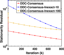
We compare the performance of the proposed algorithm DDC-Consensus with its following two relaxations: (i) DDC-Consensus-Inexact-$q$, where we solve the minimization problems (4) and (5) inexactly via a gradient descent method for $q$ iterations, (ii) DDC-Mixing, where the $\eta$-consensus is replaced with one step mixing (applying one iteration of the updates (15)-(17) to $y_{i}$ estimates of the optimization algorithms). To demonstrate the performance of the proposed algorithm we present utilize the following residual metrics: Solution Residual$(k)$: $\frac{1}{10}\sum_{i=1}^{10}\|y_{i}^{(k)}-x^{*}\|_{2}$, Stationarity Residual$(k)$: $\frac{1}{10}\sum_{i=1}^{10}\|x_{\mu g_{i}}(y_{i}^{(k)})-x_{\mu f_{i}}(y_{i}^{(k)})\|_{2}$, Objective Residual$(k)$: $F(y_{i}^{(k)})-F^{*}$, Consensus Residual$(k)$: $\frac{1}{10}\sum_{i=1}^{n}\sum_{j=1}^{n}\|y_{i}^{(k)}-y_{j}^{(k)}\|_{2}$.

IV-A Comparison with DDC-Consensus-Inexact-$q$

Figs. 1-3 demonstrate the performance comparisons between the proposed DDC-Consensus algorithm and two instances of DDC-Consensus-Inexact-$q$ that are denoted as DDC-Consensus-Inexact-$10$ and DDC-Consensus-Inexact-$100$ respectively. This comparison aims to determine a trade-off between the accuracy and computational burden of the proximal minimization in the proposed DDC-Consensus algorithm. As expected the DDC-Consensus algorithm performs the best with respect to all the performance metrics. Fig. 1 shows the stationarity metric that gives an estimate of the rate of convergence in the sense of Theorem 3.

Refer to caption
Figure 2: Objective residual comparison: proposed DDC-Consensus and DDC-Consensus-Inexact-$q$
Refer to caption
Figure 3: Solution residual comparison: proposed DDC-Consensus and DDC-Consensus-Inexact-$q$
Refer to caption
Figure 4: Stationarity residual: DDC-Consensus and DDC-Mixing

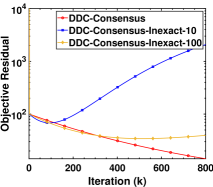
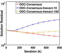
Figs. 2 and 3 show that gradient descent with a low computational footprint can perform relatively well compared to the exact minimization in the DDC-Consensus algorithm. However, it is also established that if the proximal minimization is not performed with good accuracy the algorithm iterates to diverge as in the case of DDC-Consensus-Inexact-$10$.

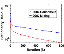
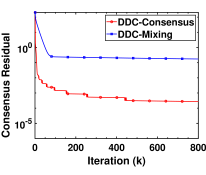
IV-B Comparison with DDC-Mixing

Figs. 4-7 present comparison plots showing the different metrics for both the DDC-Consensus and DDC-Mixing algorithms.

Refer to caption
Figure 5: Objective residual: DDC-Consensus and DDC-Mixing

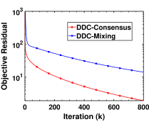
The simulation study in this section aims to study the effect of the agreement quality between the agent estimates in the DDC-Consensus algorithm on its performance. The DDC-Mixing algorithm uses only one information exchange step among the agents and is theoretically the lower bound on information aggregation. Note, that both DDC-Consensus and DDC-Mixing algorithms perform exact proximal minimization steps.
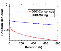
Refer to caption
Figure 6: Solution residual comparison: proposed DDC-Consensus and DDC-Mixing

Figs. 4-6 show that the $\eta$-consensus protocol allows for a higher degree of agreement between the agent estimates during the algorithm iterations lead to better convergence properties of the proposed DDC-Consensus algorithm compared to the DDC-Mixing algorithm. Furthermore, the $\eta$-consensus protocol adaptively controls the agent mismatch and leads to the consensus constraint satisfaction at every iterate of the proposed DDC-Consensus algorithm as seen in Fig. 7.

Refer to caption
Figure 7: Consensus residual: DDC-Consensus and DDC-Mixing

V Conclusion

We focused on a distributed DC optimization problem with local objective functions given by the difference between a nonsmooth weakly convex function and a nonsmooth convex function. Based on the gradient of the smooth approximations of the weakly convex and convex functions we developed the distributed DDC-Consensus algorithm. In the DDC-Consensus algorithm each agent performs a local gradient descent step and updates its estimates using a finite-time $\eta$-consensus protocol. The agent estimates are shared over a directed graph and updated via a column stochastic matrix; giving DDC-Consensus the desirable properties of allowing for non-symmetric communication and distributed synthesis. We established that the DDC-Consensus algorithm converges to a stationary point of the nonconvex distributed optimization problem. The numerical performance of the DDC-Consensus algorithm is presented in a simulation study solving the DC-regularized least squares problem. Results showing the behavior of DDC-Consensus and its relaxations DDC-Consensus-Inexact-$q$ and DDC-Mixing concerning the residual metrics demonstrate the efficacy of the proposed DDC-Consensus algorithm.

References

  • [1] V. Khatana and M. V. Salapaka, “D-distadmm: A o(1/k) distributed admm for distributed optimization in directed graph topologies,” in 2020 59th IEEE Conference on Decision and Control (CDC), 2020, pp. 2992–2997.
  • [2] V. Khatana, G. Saraswat, S. Patel, and M. V. Salapaka, “Gradient-consensus method for distributed optimization in directed multi-agent networks,” in 2020 American Control Conference (ACC), 2020, pp. 4689–4694.
  • [3] P. Hartman, “On functions representable as a difference of convex functions.” Pacific Journal of Mathematics, vol. 9, no. 3, pp. 707–713, 1959.
  • [4] M. Nouiehed, J.-S. Pang, and M. Razaviyayn, “On the pervasiveness of difference-convexity in optimization and statistics,” Mathematical Programming, vol. 174, no. 1, pp. 195–222, 2019.
  • [5] S. Merkli, A. Domahidi, J. L. Jerez, M. Morari, and R. S. Smith, “Fast ac power flow optimization using difference of convex functions programming,” IEEE Transactions on Power Systems, vol. 33, no. 1, pp. 363–372, 2017.
  • [6] H. An and L. Thi, “Solving large scale molecular distance geometry problems by a smoothing technique via the gaussian transform and dc programming,” Journal of Global Optimization, vol. 27, no. 4, pp. 375–397, 2003.
  • [7] T. H. L. An and P. D. Tao, “Dc optimization approaches via markov models for restoration of signal (1-d) and (2-d),” in Advances in Convex Analysis and Global Optimization.   Springer, 2001, pp. 303–317.
  • [8] L. T. Hoai An and P. D. Tao, “Dc programming approach for multicommodity network optimization problems with step increasing cost functions,” Journal of Global Optimization, vol. 22, no. 1, pp. 205–232, 2002.
  • [9] H. A. Le Thi and T. P. Dinh, “A continuous approch for globally solving linearly constrained quadratic,” Optimization, vol. 50, no. 1-2, pp. 93–120, 2001.
  • [10] J. N. Tsitsiklis, “Problems in decentralized decision making and computation.” Massachusetts Inst of Tech Cambridge Lab for Information and Decision Systems, Tech. Rep., 1984.
  • [11] D. P. Bertsekas and J. N. Tsitsiklis, Parallel and distributed computation: numerical methods.   Prentice hall Englewood Cliffs, NJ, 1989, vol. 23.
  • [12] S. Pu, W. Shi, J. Xu, and A. Nedic, “Push-pull gradient methods for distributed optimization in networks,” IEEE Transactions on Automatic Control, 2020.
  • [13] V. Khatana and M. V. Salapaka, “Dc-distadmm: Admm algorithm for constrained optimization over directed graphs,” IEEE Transactions on Automatic Control, vol. 68, no. 9, pp. 5365–5380, 2023.
  • [14] V. Khatana, G. Saraswat, S. Patel, and M. V. Salapaka, “Gradconsensus: Linearly convergent algorithm for reducing disagreement in multi-agent optimization,” IEEE Transactions on Network Science and Engineering, vol. 11, no. 1, pp. 1251–1264, 2024.
  • [15] J. Zeng and W. Yin, “On nonconvex decentralized gradient descent,” IEEE Transactions on Signal Processing, vol. 66, no. 11, pp. 2834–2848, 2018.
  • [16] R. Xin, U. A. Khan, and S. Kar, “A fast randomized incremental gradient method for decentralized nonconvex optimization,” IEEE Transactions on Automatic Control, vol. 67, pp. 5150–5165, 2020. [Online]. Available: https://api.semanticscholar.org/CorpusID:226282498
  • [17] Y. Yan, C. Niu, Y. Ding, Z. Zheng, F. Wu, G. Chen, S. Tang, and Z. Wu, “Distributed non-convex optimization with sublinear speedup under intermittent client availability,” INFORMS J. Comput., vol. 36, pp. 185–202, 2020. [Online]. Available: https://api.semanticscholar.org/CorpusID:211146497
  • [18] G. Scutari and Y. Sun, “Distributed nonconvex constrained optimization over time-varying digraphs,” Mathematical Programming, vol. 176, pp. 497–544, 2019.
  • [19] E. Gorbunov, K. P. Burlachenko, Z. Li, and P. Richtárik, “Marina: Faster non-convex distributed learning with compression,” in International Conference on Machine Learning.   PMLR, 2021, pp. 3788–3798.
  • [20] X. Jiang, X. Zeng, J. Sun, and J. Chen, “Distributed proximal gradient algorithm for nonconvex optimization over time-varying networks,” IEEE Transactions on Control of Network Systems, vol. 10, no. 2, pp. 1005–1017, 2023.
  • [21] P. D. Lorenzo and G. Scutari, “Next: In-network nonconvex optimization,” IEEE Transactions on Signal and Information Processing over Networks, vol. 2, pp. 120–136, 2016. [Online]. Available: https://api.semanticscholar.org/CorpusID:3261082
  • [22] S. Chen, A. García, and S. Shahrampour, “On distributed nonconvex optimization: Projected subgradient method for weakly convex problems in networks,” IEEE Transactions on Automatic Control, vol. 67, pp. 662–675, 2020. [Online]. Available: https://api.semanticscholar.org/CorpusID:234356225
  • [23] A. Alvarado, G. Scutari, and J.-S. Pang, “A new decomposition method for multiuser dc-programming and its applications,” IEEE Transactions on Signal Processing, vol. 62, no. 11, pp. 2984–2998, 2014.
  • [24] H. Le Thi, DC Programming and DCA.   (Homepage), 2005. [Online]. Available: http://www.lita.univ-lorraine.fr/~lethi/index.php/en/research/dc-programming-and-dca.html
  • [25] H. A. Le Thi, T. P. Dinh, H. M. Le, and X. T. Vo, “Dc approximation approaches for sparse optimization,” European Journal of Operational Research, vol. 244, no. 1, pp. 26–46, 2015.
  • [26] P. D. Tao and L. H. An, “Convex analysis approach to dc programming: theory, algorithms and applications,” Acta mathematica vietnamica, vol. 22, no. 1, pp. 289–355, 1997.
  • [27] L. T. H. An and P. D. Tao, “The dc (difference of convex functions) programming and dca revisited with dc models of real world nonconvex optimization problems,” Annals of operations research, vol. 133, pp. 23–46, 2005.
  • [28] M. Ahn, J.-S. Pang, and J. Xin, “Difference-of-convex learning: directional stationarity, optimality, and sparsity,” SIAM Journal on Optimization, vol. 27, no. 3, pp. 1637–1665, 2017.
  • [29] P. D. Nhat, H. M. Le, and H. A. Le Thi, “Accelerated difference of convex functions algorithm and its application to sparse binary logistic regression.” in IJCAI, 2018, pp. 1369–1375.
  • [30] T. Sun, P. Yin, L. Cheng, and H. Jiang, “Alternating direction method of multipliers with difference of convex functions,” Advances in Computational Mathematics, vol. 44, pp. 723–744, 2018.
  • [31] K. Sun and X. A. Sun, “Algorithms for difference-of-convex programs based on difference-of-moreau-envelopes smoothing,” INFORMS Journal on Optimization, vol. 5, no. 4, pp. 321–339, 2023.
  • [32] B. Wen, X. Chen, and T. K. Pong, “A proximal difference-of-convex algorithm with extrapolation,” Computational optimization and applications, vol. 69, pp. 297–324, 2018.
  • [33] R. T. Rockafellar and R. J.-B. Wets, Variational analysis.   Springer Science & Business Media, 2009, vol. 317.
  • [34] V. Yadav and M. V. Salapaka, “Distributed protocol for determining when averaging consensus is reached,” in 45th Annual Allerton Conf, 2007, pp. 715–720.
  • [35] M. Prakash, S. Talukdar, S. Attree, S. Patel, and M. V. Salapaka, “Distributed stopping criterion for ratio consensus,” in 2018 56th Annual Allerton Conference on Communication, Control, and Computing (Allerton), 2018, pp. 131–135.
  • [36] M. Prakash, S. Talukdar, S. Attree, V. Yadav, and M. V. Salapaka, “Distributed stopping criterion for consensus in the presence of delays,” IEEE Transactions on Control of Network Systems, vol. 7, no. 1, pp. 85–95, 2020.
  • [37] J. Melbourne, G. Saraswat, V. Khatana, S. Patel, and M. V. Salapaka, “On the geometry of consensus algorithms with application to distributed termination in higher dimension,” in the proceedings of International Federation of Automatic Control (IFAC), 2020. [Online]. Available: http://box5779.temp.domains/~jamesmel/wp-content/uploads/2019/11/Vector_Consensus__IFAC_-1.pdf
  • [38] ——, “Convex decreasing algorithms: Distributed synthesis and finite-time termination in higher dimension,” IEEE Transactions on Automatic Control, vol. 69, no. 6, pp. 3960–3967, 2024.
  • [39] D. Kempe, A. Dobra, and J. Gehrke, “Gossip-based computation of aggregate information,” in 44th Annual IEEE Symposium on Foundations of Computer Science, 2003. Proceedings.   IEEE, 2003, pp. 482–491.
  • [40] G. Saraswat, V. Khatana, S. Patel, and M. V. Salapaka, “Distributed finite-time termination for consensus algorithm in switching topologies,” IEEE Transactions on Network Science and Engineering, vol. 10, no. 1, pp. 489–499, 2023.
  • [41] P. Erdős and A. Rényi, “On the evolution of random graphs,” Publ. Math. Inst. Hung. Acad. Sci, vol. 5, no. 1, pp. 17–60, 1960.