Fluorescence Diffraction Tomography using Explicit Neural Fields

Abstract

Solving the 3D refractive index (RI) from fluorescence images provides both fluorescence and phase information about biological samples. However, accurately retrieving the phase of partially coherent light to reconstruct the unknown RI of label-free phase objects over a large volume, at high resolution, and in reflection mode remains challenging. To tackle this challenge, we developed fluorescence diffraction tomography (FDT) with explicit neural fields that can reconstruct 3D RI from defocused fluorescence speckle images. The successful reconstruction of 3D RI using FDT relies on four key components: coarse-to-fine modeling, self-calibration, a differential multi-slice rendering model, and partial coherent masks. Specifically, the explicit representation efficiently integrates with the coarse-to-fine modeling to achieve high-speed, high-resolution reconstruction. Moreover, we advance the multi-slice equation to differential multi-slice rendering model, which enables the self-calibration method for the extrinsic and intrinsic parameters of the system. The self-calibration facilitates high accuracy forward image prediction and RI reconstruction. Partial coherent masks are digital masks to resolve the discrepancies between the coherent light model and the partial coherent light data accurately and efficiently. FDT successfully reconstructed the RI of 3D cultured label-free 3D MuSCs tube in a 530 $\times$ 530 $\times$ 300 $\mu m^{3}$ volume at 1024$\times$1024 pixels across 24 $z$-layers from fluorescence images, demonstrating high fidelity 3D RI reconstruction of bulky and heterogeneous biological samples in vitro.

1 Introduction

Fluorescence and phase microscopy are two powerful techniques in the field of biological imaging, providing essential insights into the molecular specificity and quantitative biophysical properties of biological samples. Fluorescence microscopy captures molecular specified structural and functional information through exogenous fluorescence labeling or intrinsic autofluorescence. Phase microscopy quantitatively evaluate the biophysical properties of biological samples by measuring their refractive index (RI). Combining these distinct imaging modalities to image the same sample allows for studying the correlation between fluorescence-labeled structures and label-free structures with heterogeneous RI [1, 2, 3, 4, 5, 6].

optical diffraction tomography (ODT) [7, 8], as a quantitative phase imaging (QPI), can recover 3D RI distribution of a sample. Intensity diffraction tomography (IDT) [9, 10] can be seen as an advanced form of ODT that utilizes interferometric methods to enhance the accuracy and resolution of the 3D reconstruction. The challenge of traditional ODT methods lies in the computational complexity of processing large volumes of high-resolution images using traditional methods, which often leads to inefficiencies. Moreover, most of ODT methods use transmitted light, which limits the noninvasive application of the method. Despite these difficulties in phase retrieval, combining phase image with fluorescence brings additional challenges. Given the significance of integrating fluorescence and phase imaging, several techniques [3, 4, 5, 6, 11, 12] have been developed in the last decade. However, these methods combine two separate setups for sequential imaging, limiting their potential on simultaneously fluorescent and phase imaging of transient dynamics.

Many deep learning-based methods for phase recovery have been developed [13, 14]. A classic approach is to train an end-to-end neural network, such as a convolutional neural network (CNN) [15], to directly retrieve the phase from the input images. However, these end-to-end strategies typically require large and high-quality datasets and face general issues related to generalizability and accuracy. Although neural networks can be seen as inverse problem solvers [16] in function form, it remains unclear how the network operates, resulting in lower interpretability. Recently, the development of physically informed neural networks (PINNs) [17] and neural radiance fields (NeRFs) [18] has offered new ways to solve ill-posed inverse problems without the requirement of large dataset. Combining simple neural networks with physical principles significantly enhances the interpretability. Some papers have leveraged these new paradigm to solve the phase retrieval problem. For instance, Liu et al. [19] combined neural fields with the Born approximation to solve the RI from discrete intensity-only measurements, and Zhou et al. [20] integrated neural fields with Fourier ptychographic microscopy to solve the phase and achieve super-resolution. However, due to the nature of implicit representations, which encode unknown RI into the network rather than directly solving it, these networks struggle to handle strong nonlinearity or sharp gradient issues that are very common for PINNs [21].

More recently, our group [1, 2] proposed a 3D bi-functional refractive index and fluorescence microscopy (BRIEF), that enables simultaneous fluorescence and phase imaging in a reflection mode for the first time. Unlike the methods in transmission mode [3, 4, 5, 6] , BRIEF acquires dozens of fluorescence images in reflection mode, each ‘illuminated’ by a single fluorophore, then solve an inverse problem with a multiple-scattering forward model. However, BRIEF requires contrived samples with sparsely distributed fluorophores to avoid crosstalk between measurements under one-photon excitation. Compared to the plane wave used in ODT, BRIEF uses spatially variant spherical wave from individual fluorophores inside the sample, which enables optical sectioning but also requires precise modeling. This makes it challenging to model the intensity and location of the partially coherent illumination source. In terms of computational efficiency, BRIEF encounters similar challenges to traditional ODT methods in handling large numbers of high-resolution images due to the computational burden.

To address these limitations, we develop two-photon excited fluorescence diffraction tomography (FDT) with explicit neural fields. It uses two-photon excited fluorescence as illumination sources, lifts the constraint of sparse fluorescence labeling, and solves the 3D RI using the neural fields method with an explicit representation. The main contributions of our method are as follows:

1. We develop an explicit representation for RI reconstruction and combine it with coarse-to-fine modeling, enabling fast and high-resolution reconstruction.

2. We develop a self-calibration method to localize the positions of fluorescence sources in 3D, achieving highly accurate forward image prediction.

3. We derive and implement a differential multi-slice model within a neural network framework, ensuring all parameters are differentiable and irretrievable, which enables explicit representation, self-calibration, and further post-processing.

4. We design a partial coherent mask to resolve the model discrepancy between the coherent illumination of the multi-slice model and the partial coherent experimental data.

5. We design the FDT in reflection mode to achieve high-quality 3D RI reconstruction of bulky biological samples.

In this paper, We validate FDT and quantitatively evaluate the performance with simulated results and experimental data. We successfully reconstruct the 3D RI of thin-layers of Madin-Darby Canine Kidney (MDCK) GII cells and bulky 3D cultured microtube formed with Bovine muscle stem cells (MuSCs) from defocused two-photon fluorescence images. To our knowledge, FDT is the first method to achieve diffraction tomography from two-photon excited fluorescence. FDT significantly advances fluorescence-phase multimodal imaging and providing deeper insights into the function and structure of biological samples.

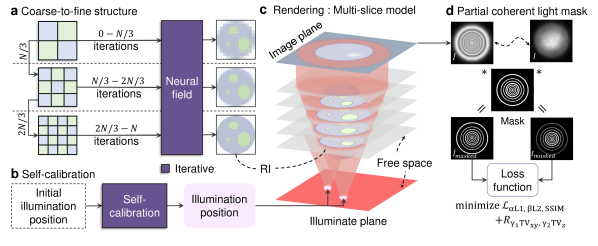
Figure 1: Overview of FDT using explicit neural fields. a, The refractive index (RI) is generated by the neural fields model and refined through three stages with increasing resolutions at different iterations using coarse-to-fine modeling. b, Self-calibration is applied to localize the illuminator positions, starting from an initial estimation by Gaussian fitting. The values are then set as iterative parameters and optimized during the training process. c, The rendering equation is based on the differential multi-slice model, which takes two inputs: the RI from a and the illuminator positions from b. This model describes how light propagates through homogeneous media and heterogeneous biological tissue, and be captured on the image plane. d, A partial coherent light mask is generated by computing light propagation to the image plane through the multi-slice model without heterogeneous RI (”free space”) and then binarized and applied to the predicted and measured images. The masked images are used to calculate the loss function, incorporating L1, L2, SSIM, and regularization terms.

2 Results

In this section, we first explain the details of our FDT model, as illustrated in Fig. 1 and validate our model and its components using simulation data, as discussed in Section 2.1. Finally, we apply FDT to take experimental images and reconstruct 3D RI from both thin (Section 2.2.1) and thick (Section 2.2.2) biological samples to demonstrate the model’s effectiveness across various structures and its capability in optical sectioning.

2.1 Model validation

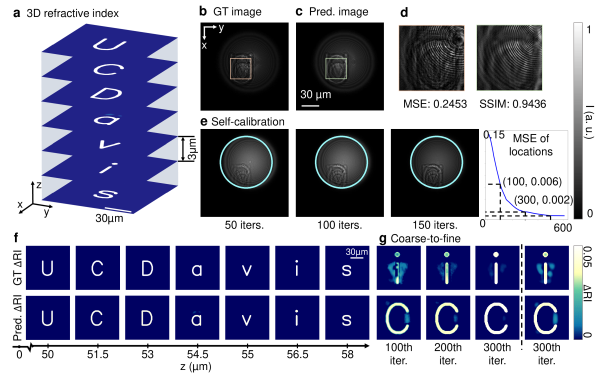
Figure 2: Reconstruction of simulated “UCDavis” pattern. a, 3D RI distribution of the ”UCDavis” pattern in 3D. b, Ground-truth (GT) image, generated using the multi-slice model with the known 3D RI distribution. c, Predicted image, generated by FDT simulation. d, Magnified views of the regions within the orange and green boxes in b and c, respectively. The MSE, SSIM between the ground-truth and predicted images are 0.2453 and 0.9436, respectively. e, Effect of self-calibration on illuminator position over 50, 100, and 150 iterations. The blue circles indicate the ground-truth illuminator position. The plot on the right illustrates the MSE loss between the self-calibrated and ground-truth illuminator positions, converging to 0.001 within 500 iterations, indicating a successful self-calibration of illuminator positions. f, Comparison of the ground-truth RI (first row) and the predicted RI (bottom row) on each $z$ plane, as indicated by the axis below. g, Effect of the coarse-to-fine modeling on reconstruction results. The first three columns show results of the coarse-to-fine modeling at different iterations (100, 200, and 300) with progressively increasing resolutions of 128$\times$128, 256$\times$256, and 512$\times$512. The last column shows the results after 300 iterations without the coarse-to-fine modeling at a resolution of 512$\times$512. Images reconstructed without the coarse-to-fine modeling exhibit artifacts and suffer from the miss DC frequency problem, demonstrating the effectiveness of the coarse-to-fine modeling in achieving higher-quality reconstructions.

In this subsection, we assess the validity of our method’s core components through evaluations on simulated datasets. The motivation for employing simulated data due to the inherent challenges associated with acquiring accurate ground-truth information in real experiments, such as illumination position and RI. Consequently, to preliminarily validate our algorithm’s validation and effectiveness, we test the performance of each components of FDT on the simulated data, indirectly substantiates the algorithm’s potential applicability to real-world scenarios.

We first validate our method by reconstructing the 3D RI of a “UCDavis” pattern, Fig. 2.

The ground-truth RI of the “UCDavis” pattern consists of seven layers with a resolution of 512 $\times$ 512 pixels, where each letter in “UCDavis” is located at the center of different layers along the z-axis. We use the ground-truth RI to generate 400 ground-truth images under different illuminations.

Our model is then trained based on the ground-truth images to predict the RI and generate the predicted images based on the predicted RI. Following the Fig.1, we first definite 3D grids of RI Fig.1a, then initial the illumination position by applying Gaussian fitting on the Ground-truth images, Fig.1b. The differentiable multi-slice model (Fig. 1c) takes the RI and the illuminator positions as the input and generates the forward images. Also the differentiable multi-slice model generate reference images based on the homogeneous media. The reference images are used to calculate the partial coherent masks, detailed in 2.1.4. The masks are applied to the predicted and ground-truth images. We calculate the loss function between the predicted and ground-truth images.

Figure 2a shows the predicted RI results of the “UCDavis” pattern, where each letter has a clear shape and no crosstalk between letters on the adjacent planes. This demonstrates that our model can correctly solve the RI and clearly distinguish each letter along the z-axis from the images. Figure 2b, c, d shows the ground-truth images and predicted images, along with zoomed-in views of the indicated boxes. The MSE and SSIM between these two images are 0.2453 and 0.9436, respectively. Figure 2d further details our results for each letter. We also demonstrate another example of reconstructing the RI of beads in the supplementary material. These results demonstrate that our model is not only amenable to accurately predict the RI but also generate similar predicted images.

In the following subsection, we conduct an ablation study and discuss the validation for each component of our method. In the comparison experiments, we did not compare our method with traditional methods like [1, 22] or implicit neural networks like [18, 19]. Because these methods are based on very different optical setups without utilizing two-photon excited fluorescence as illumination sources and reconstructing 3D RI from fluorescent images.

2.1.1 Coarse-to-fine modeling

The coarse-to-fine model divides the training process into three stages, gradually increasing the resolution throughout the training. In the simulation experiments, the total training iteration is 300. In the first 100 iterations, we use the lowest sampling resolution of 128 $\times$ 128 pixels to model the unknown RI. For the subsequent 100-200 iterations, we increase the sampling resolution to 256 $\times$ 256 pixels. Finally, for the 200-300 iterations, we use the highest sampling resolution of 512 $\times$ 512 pixels. At the transition points, we employ bilinear interpolation to downsample the RI to ensure smooth transitions between different resolutions. Both experiments are trained using the Adam optimizer with a learning rate of $5e-3$ and take approximately 20 minutes for 300 iterations.

Figure 2f compares the results of the coarse-to-fine modeling with those obtained without using this approach. The left three columns illustrate the predicted RI of the letters ‘i’ and ‘C’ in “UCDavis” at 100, 200, and 300 iterations, respectively. The resolutions are gradually increased for both the RI and the images, with corresponding sampling resolutions of 128$\times$128, 256$\times$256, and 512$\times$512. The right column shows the results at 300 iterations without employing the coarse-to-fine modeling. In this case, crosstalk appears in the RI map of ‘i’ and ‘C’, indicating the coarse-to-fine modeling enhances the $z$-sectioning ability. Additionally, many methods for high-resolution RI reconstruction suffer from the missing DC frequency problem. The dot of the ‘i’ clearly shows that the results without the coarse-to-fine approach experience a loss of low-frequency detail. Figure 2f demonstrates that our coarse-to-fine modeling effectively reconstructs low frequency structures, resulting in higher quality reconstructions.

2.1.2 Self-calibration on illuminator positions and intrinsic parameters of optical system

Since the illumination is related to the phase for each point, minor inaccuracies in the positioning of the illumination source can result in substantial cumulative errors in the forward images. To address this challenge, we have developed the self-calibration methodology that optimizes the initial illuminator positions automatically with the training process, Compared to other self-calibration methods used in ODT [6, 23] , our method doesn’t require additional computation or optical setup.

We validate the self-calibration method by localizing fluorescence sources in the simulation. The ground-truth location is randomly draw from a Gaussian distribution to add uncertainty to the positions, in Fig. 2e.

The uncertain positions of fluorescence sources are defined as $\hat{p}_{i}=p_{i}+\mathcal{N}(0,\sigma^{2})$, where $\hat{p}_{i}$ represents the uncertain positions of fluorescence sources, $p_{i}$ denotes the ground-truth positions, and $\mathcal{N}(0,\sigma^{2})$ is the Gaussian noise with mean 0 and variance $\sigma^{2}$. The standard deviation $\sigma$ is set to 0.1 because the location values are normalized to the range $[-0.5,0.5]$. In this normalized range, a standard deviation of 0.1 is relatively significant, ensuring a noticeable perturbation to test the robustness of the self-calibration method.

In the training process, self-calibration begins by fitting a 2D Gaussian function to the defocused fluorescence to initialize the positions of the fluorescence sources. These positions are then set as iterative parameters that are updated throughout the training process. Figure 2f shows the results of self-calibration during the training process. The illuminated area in the predicted fluorescence image gradually aligns with that under the fluorescence illumination from the ground-truth position (blue circle). This indicates that the estimated positions of fluorescence sources are gradually converging to the ground-truth positions. The MSE plot of the positions further confirms this trend, showing a sharp decrease in MSE as the number of iterations increases, ultimately stabilizing at a lower error value. This consistent reduction in MSE reflects the effectiveness of the self-calibration process in refining the estimated positions of fluorescence sources.

This self-calibration method leverages the robustness of Gaussian fitting to provide a strong starting point, while the iterative training process ensures that the illuminator positions are accurately calibrated to enhance the overall model performance.

The self-calibration on illuminator positions leverages the robustness of Gaussian fitting to provide a strong starting point, while the iterative training process ensures that the illuminator positions are accurately calibrated to enhance the overall model performance. Moreover, we extend the self-calibration method to optical parameters such as the $dx$ and $dy$ of the system which represent the corresponding physical size for each pixel and the free space.

2.1.3 Differential multi-slice model

We extend the conventional multi-slice model [1] to a differentiable version within the PyTorch framework. BRIEF [1] struggled to handle a large number of high-resolution images because it employed a gradient-based optimization method that generates all images simultaneously. Moreover, these methods involved manually performing inverse calculations, which are not computationally efficient and have limited scalability. Consequently, these methods were restricted to optimizing only RI with given resolution. We overcome these limitations by developing a differentiable multi-slice model within the neural network framework. Firstly, we can conduct batch training with automated backpropagation, which is more computationally efficient than previous methods. Additionally, the differentiable model and automated backpropagation mechanisms allow us to arbitrarily adjust the model’s parameters. This flexibility enables us to fine-tune the RI resolution for a coarse-to-fine strategy and set the illuminator positions as parameters to facilitate self-calibration.

The principle of our approach is based on the multi-slice model used in BRIEF, which simulates the propagation of the spherical light through layers of a sample. Equation 1 mathematically models the electric field $y_{k-1}$ from the $(k-1)$th layer propagating through the $k$th layer, where the RI is $n_{k}$:

$$y_{k}=\exp\left(\frac{j2\pi}{\lambda}\Delta z(n_{k}(\mathbf{r})-n_{b})\right)\mathcal{F}^{-1}\left\{Q\cdot\mathcal{F}\{y_{k-1}\}\right\}$$ (1)

where

$$Q=\exp\left(-j\Delta z\left(\left(\frac{2\pi}{\lambda}\right)^{2}-|\mathbf{k}|^{2}\right)^{1/2}\right)$$ (2)

Upon traversing $N$ layers, the electric field at the imaging plane is given by Equation 3:

$$E(\mathbf{r})=\mathcal{F}^{-1}\left\{p(\mathbf{k})\cdot\mathcal{F}\{y_{N}(\mathbf{r})\}\right\},$$ (3)

where $p(\mathbf{k})$ is the optical system’s pupil function, and $\mathcal{F}$ and $\mathcal{F}^{-1}$ denote the Fourier transform and its inverse, respectively.

The resultant intensity distribution on the image plane, $I(\mathbf{r})$, is defined as the squared magnitude of the electric field:

$$I(\mathbf{r})=|E(\mathbf{r})|^{2}.$$ (4)

This mathematical model enables the simulation of the electric field’s propagation through the layers of a sample within the PyTorch framework. However, a significant limitation of almost all models is their foundational assumption of coherent light. In contrast, the light source for two-photon excitation fluorescence is partially coherent, leading to a substantial gap between the simulations and actual experiments. We will address and resolve this issue in the subsequent subsection 2.1.4.

2.1.4 Partial coherent light mask

The other challenge that prevents us from directly applying ODT methods to our scenario lies in the nature of the illumination. The fluorescence illumination is partially coherent or incoherent, while other ODT methods are based on the assumption of a coherent light source. Solving phase information from partially coherent or incoherent light is challenging. Manipulating or modeling the light source to address this would introduce optical or computational complexity to the system. Instead, we develop a digital mask to mitigate the partial coherence problem.

This approach is inspired by an unexpected observation made during our preliminary experiments: the algorithm exhibited sensitivity primarily to areas characterized by the second-order gradient. This discovery led us to a novel strategy, wherein we selectively focus on these sensitive regions while excluding irrelevant areas, which mainly consist of the part of the incoherent light (Fig. 1d).

First, we generate reference illumination profiles by setting the RI to 1.33. Using these profiles, we employ a local maximum searching method to identify each bright ring. The bright rings near the center of the profiles appear close together, resembling a continuous region. We select all the pixels in this smooth region. Outside of the smooth region, where the gaps between the bright rings are evident, we select only the regions of bright rings. We can dynamically generate the mask for different illumination locations in each iteration and combine with the self-calibration method. This approach effectively alleviates the effects of the incoherence of the illumination, thereby offering a solution to the problem caused by partially coherent light. Our method is general, robust, and computationally efficient.

2.2 Method evaluation

In this section, we evaluate our method by apply it to real biological samples, such as MDCK cells and a 3D MuSCs tube. The label-free cells are cultured on a coverslip-bottom dish, with fluorescence sprayed on the outside.We spray one side of the coverslip with a fluorescent dye and then place the sample on the other side. The details of the sample preparation can be found in Section 3.1.3.

2.2.1 MDCK Cells 3D RI Reconstruction and Analysis

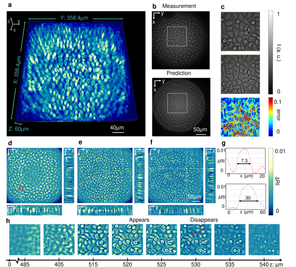
Figure 3: 3D RI Reconstruction of a MDCK sample. a, 3D visualization of the RI distribution within a volume of 358.4 $\times$ 358.4 $\times$ 60 $\mu m^{3}$ . b, Comparison of the measured (top) and predicted (bottom) images, with a highlighted region of interest. c, Detailed views of the highlighted region: measured image (top), predicted image (middle), and error map (bottom). d-f, Cross-sectional views of the RI difference distribution on different planes ($xy$, $xz$, $yz$), illustrating spatial variations in RI. g, Quantitative analysis of RI variation of the red box in d, showing RI along the X-axis (top) and Z-axis (bottom). h, Sequence of images highlighting the appearance and disappearance of specific features within the region along the Z-axis.

Figure 3 presents the recon for MDCK cells. The reconstruction result is shown in Fig. 3a, which consists of 12 slices with a resolution of 1024 $\times$ 1024 pixels, forming a volume of $358.4\times 358.4\times 60~{}\mu m^{3}$. The FDT method not only successfully recovers the sample’s structure, but also demonstrate high accuracy in the forward images as seen in Fig 3b. Fig 3c provides zoomed-in details of Fig. 3b, where we can further distinguish intracellular structures of the cells. In the error map at the bottom, we can see that the error is very small, with the highest values mostly distributed in the background, while the cell regions are of high accuracy. These accurate forward images are fundamental to the successful RI reconstruction. Figure 3d-f show three cross-sectional views of the RI difference in the $xy$, $xz$, and $yz$ planes. The clear shapes of the cells and distinct edges between them highlight the high resolution in both the $xy$ plane and along the $z$-axis. Figure 3g illustrates the RI variation within the red box shown in Fig. 3d. Figure 3h displays the $xy$ sections from different $z$ planes. As the $z$ value increases, cells can be observed appearing and disappearing. In the last several layers, brighter cells, which are dead cells, are visible. These cells are shrunken and floating above the substrate, indicating a higher RI and less adherence to the bottom. This feature serves as evidence of our method’s $z$-sectioning capability and RI sensitivity.

Table 1: Performance metrics w/ and w/o the mask for the MDCK reconstruction result.

Method	SSIM	PSNR	PCC
w/ mask	0.8194	28.2157	0.0665
w/o mask	0.8177	28.7119	0.0594

The quantitative analysis of our method’s performance is summarized in Table 1 w/ mask. The SSIM is 0.8194, reflecting high structural similarity between the predicted and ground-truth images.

2.2.2 MuSCs tube 3D RI Reconstruction and Analysis

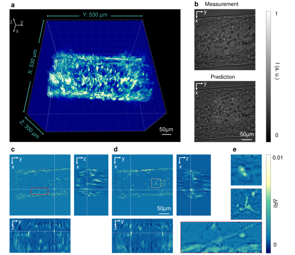
Figure 4: 3D RI Reconstruction of a 3D MuSCs tube sample. a, 3D visualization of the RI distribution within a volume of $530\times 530\times 300~{}\mu m^{3}$. b, Comparison of the measured (top) and predicted (bottom) images, highlighting a region of interest. c-d, Cross-sectional views of the RI difference distribution along different planes ($xy$, $xz$, $yz$), illustrating spatial variations in RI. e, Zoomed-in details of the highlighted regions in c and d, showing three different morphological fine structures and variations in RI: the top image corresponds to the green box in (d), the middle image to the orange box in (d), and the bottom image to the red box in (c).

Figure 4 presents the results for a 3D MuSCs tube sample. The reconstruction result is shown in Fig. 4a, which consists of 24 slices with a resolution of 1024 $\times$ 1024 pixels, forming a volume of $530\times 530\times 300~{}\mu m^{3}$. The FDT method successfully recovers the thick sample’s structure, demonstrating the ability of our method to handle large volumes and thick samples. Even under suboptimal fluorescence illumination conditions, our method can handle a larger volume compared to the state-of-the-art IDT methods [1, 24, 19].

Figure 4b demonstrates the high accuracy in forward image prediction, where we can easily distinguish between defocused and in-focus regions. Specifically, the defocused cells in the center appear with dark centers, while the in-focus cells show bright centers. This differentiation indicates the precision of our FDT method in RI reconstruction, validating the method’s potential for high-fidelity reconstructions.

Cross-sectional views presented in Fig. 4c and 4d further elucidate the structure of the 3D MuSCs tube sample. These slices, taken in the $xy$, $xz$, and $yz$ planes, reveal the sample’s tubular morphology. The circular cross-section observable in the $xz$ plane confirms the integrity of the tube structure, while the clear delineation between the top and bottom of the tube underscores our method’s effective $z$-sectioning ability. This ability to maintain structural fidelity across different planes is crucial for accurate 3D reconstructions.

Zoomed-in views of selected regions (Fig. 4e) provide insights into the fine morphological structures and RI variations within the sample. The top image, corresponding to the green box in Fig. 4d, highlights two closely positioned cells, demonstrating the high spatial resolution achieved by our model. The middle image, associated with the orange box in Fig. 4d, reveals muscle cells in the process of forming intercellular junctions, a detail that underscores our method’s capability to capture fine biological processes. The bottom image, derived from the red box in Fig. 4c, clearly shows the edge of the 3D tube wall composed of multiple muscle cells, highlighting the method’s ability to resolve diversity structural details.

Overall, these results collectively demonstrate the robustness, accuracy, and high resolution of our FDT method in reconstructing complex biological samples, offering significant improvements over existing imaging techniques.

2.3 Discussion

We develop FDT, a new multimodal imaging technique, for reconstructing 3D RI from fluorescence images using the explicit neural field and incorporates several innovative and efficient components. We designed a coarse-to-fine strategy for 3D RI reconstruction, developed a self-calibration method to accurately determine the illumination position and optical parameters, which were previously difficult to acquire, and designed a partial coherent mask to address the model mismatching problem. Our method can achieve a maximum depth of 300 $\mu m$ in the $z$-direction within one hour and attain 90% of the best result in just 20 minutes. This demonstrates that our approach is not only more robust but also faster than the current state-of-the-art methods.

The coarse-to-fine strategy significantly enhances the speed and resolution of the 3D RI reconstruction. This makes our method not only faster and more interpretable but also adaptable for future advancements such as the octree structure [25]. The self-calibration method is a versatile approach used in computational imaging methods. In our method, the foundation of self-calibration is the differential multi-slice model, where each variable is irretrievable. Due to its plug-and-play and computational efficiency features, we believe it will be widely adopted in various methods within this field.

By integrating these components, our approach offers a robust and high-performance solution for 3D RI reconstruction, paving the way for further innovations and applications in biological imaging. Our method not only demonstrates the potential of fluorescence illumination in diffraction tomography but also sets the stage for future developments in high-speed, high-resolution imaging technologies.

Since no specific method targets the same problem we address, we compare our approach with several state-of-the-art RI reconstruction methods. Compared to our previous work BRIEF, FDT can handle dense objects and extends from one-photon to two-photon illumination, allowing for more precise excitation in 3D space. Leveraging the neural fields method, our approach utilizes thousands of images to achieve high-resolution reconstruction and effectively address the missing cone problem.

Among deep learning-related methods, one notable work is DeCAF [19], which also achieves high-resolution RI reconstruction using neural fields. However, The first Born approximation hinders imaging of thick samples (over hundreds of microns), and the implicit representation limits computational speed. In contrast to conventional ODT methods that use transmitted light, our method is based on fluorescence microscopy in reflection mode, opening up the possibility of in vivo imaging in the future. Further qualitative comparisons are provided in the supplementary materials.

Limitations of FDT. Although we have successfully achieved fluorescence diffraction tomography for the first time, there are still several aspects where we have not fully utilized the advantages of fluorescence illumination. For instance, our current setup includes free space between the fluorescence source and the biological sample, such as a cover slip. This setup can be optimized to create a more realistic scenario by eliminating these gaps. We plan to upgrade our model both computationally and optically to solve the 3D RI of bulky tissues without any free space. Additionally, our model currently faces a memory inefficiency issue. The number of layers that can be processed is limited by the GPU memory available. To address this, we will develop memory-efficient methods to enhance the scalability of our approach. By tackling these limitations, we aim to improve the practicality and effectiveness of FDT for more complex and realistic biological imaging scenarios.

2.4 Conclusion

Our FDT method significantly advances traditional ODT by enhancing neural field-based approaches through explicit representation, achieving high-speed, high-resolution, and high-accuracy reconstructions. Unlike traditional methods that rely on sliced samples illuminated in a transmitted mode, FDT opens new possibilities for in vivo biological and medical imaging in reflection mode. This advancement highlights the potential for real-time, high-resolution imaging of living tissues, providing valuable insights into dynamic biological processes and paving the way for future innovations in the field of diffraction tomography.

3 Method

3.1 Experimental setup

3.1.1 Optical Setting

The laser source to excite fluorophores is a femtosecond laser at 1035 nm wavelength (Monaco 1035-40-40 LX, Coherent NA Inc., U.S.). The SLM is at the conjugate Fourier plane. The phase of each beam is modulated by a spatial light modulator (SLM) (HSPDM1K-900-1200-PC8, Meadowlark Optics Inc., U.S.) to excite a fluorophore at a pre-determined position in 3D. The laser beam size is expanded after the laser source to fill the SLM fully. Then, the modulated laser beam passes through the objective lens (XLUMPLFLN20XW, 20$\times$, NA 1.0, Olympus Inc., Japan) to excite a fluorophore and generate an illumination spot. A customized dichroic mirror (FF880-SDI01-T3-35X52, Chroma, U.S.) is placed before the objective lens to reflect the stimulation laser beams to the sample while transmitting fluorescence photons emitted from the sample. The set of fluorescence images generated from fluorophores at different positions is recorded by a camera (Kinetix22, Teledyne Photometrics, U.S.) controlled by the Micro-Manager software. A filter (AT635/60m, Chroma, U.S.) is placed before the camera only to transmit fluorescence light. A NI-DAQ (National Instruments, NI PCIe-6363) synthesizes custom digital signals to synchronously modulate the laser, the SLM, and the camera. A custom MATLAB (MathWorks, U.S.) graphic user interface controls the NI DAQ boards, calibrates the system, and acquires data.

3.1.2 Computational Setting

Our model is trained on an NVIDIA A6000 GPU with 48GB Memory. We use the Adam optimizer with initial learning rate at 1e-5 with decay rate (0.9, 0.99). Batch size is 30.

loss function. The loss function utilized in this study is designed to optimize multiple aspects of the model’s performance by incorporating various components that address different error metrics and regularization terms. The formulation of the loss function is as follows:

$$\mathscr{L}(I,\hat{I},\hat{n})=\sum_{i=0}^{batch}\underbrace{\left[\begin{matrix}\alpha&\beta&1\end{matrix}\right]}_{\text{Dynamic weights}}\times\underbrace{\begin{bmatrix}w_{1}&&\\ &w_{1}&\\ &&w_{2}\end{bmatrix}}_{\text{Balance contribution}}\times\underbrace{\left[\begin{matrix}\|\mathbf{I}_{i}-\hat{\mathbf{I}}_{i}\|_{1}\\ \|\mathbf{I}_{i}-\hat{\mathbf{I}}_{i}\|_{2}^{2}\\ \ell_{ssim}(\mathbf{I}_{i},\hat{\mathbf{I}_{i}})\end{matrix}\right]}_{\text{Loss items}}$$ (5)

$$+\underbrace{\left[\begin{matrix}w_{3},&w_{4}\end{matrix}\right]}_{\text{Weights}}\times\underbrace{\left[\begin{matrix}\sum_{x=0}^{H-1}\sum_{x=0}^{W-1}\sqrt{(\hat{n}_{x+1,y}-\hat{n}_{x,y})^{2}+(\hat{n}_{x,y+1}-\hat{n}_{x,y})^{2}}\\ \sum_{z}^{layers}\sqrt{(\hat{n}_{z+1}-\hat{n}_{z})^{2}}\end{matrix}\right]}_{\text{Total variation regularizers}}.$$

Here, $I$ represents the measurements, $\hat{I}$ denotes the predicted images generated by our multislice model, and $\hat{n}$ is the predicted refractive index (RI). Each term in the loss function is weighted by specific parameters to balance their contributions according to the desired outcomes of the model.

The matrix $[\alpha\ \beta\ 1]$ represents the dynamic weights assigned to the different loss components. These weights ensure that $\alpha+\beta=1$, allowing for a balance between the terms. Initially, $\beta$ is set higher to prioritize the reduction of large errors, while $\alpha$ is gradually increased during training to emphasize sparsity and fine-tuning of the predictions. This dynamic adjustment ensures that the model initially focuses on coarse corrections before refining its outputs, providing a robust framework for achieving high-quality predictions.

The term $w_{1},w_{2}$ scale the contributions of the loss components. Here, $w_{1}$ and $w_{2}$ are hyperparameters that control the overall impact of the respective loss terms. The L1 loss represents the mean absolute error, promoting sparsity in predictions, while the L2 loss, representing the mean squared error, helps reduce large errors. These loss items are applied to the input images $I$ and $\hat{I}$.

In addition to the L1 and L2 terms, the SSIM term is included to measure the similarity between predicted and ground-truth images, capturing perceptual differences and preserving image quality. This term is scaled by $w_{2}$. Furthermore, to encourage smoothness in the image along the $x$, $y$, and $z$ axes, we incorporate Total Variation (TV) regularization terms. The vector $[w_{3},w_{4}]$ controls the contribution of these total variation terms.

The first integral term represents the total variation in the $xy$ plane, promoting spatial consistency and reducing noise. The second integral term represents the total variation along the $z$ axis, further promoting smoothness. By combining these components, the loss function aims to balance accuracy, perceptual quality, and regularization.

The hyperparameters $w_{1}$, $w_{2}$, $\alpha$, $w_{3}$, and $w_{4}$ are meticulously tuned to optimize performance for the specific application. This dynamic adjustment of $\alpha$ and $\beta$ during training ensures that the model initially focuses on coarse corrections before refining its outputs, providing a robust framework for achieving high-quality predictions.

Evaluation metrics. The evaluation metrics used in this study include MSE, which measures the average squared differences between predicted and actual values; SSIM, which assesses perceptual similarity considering luminance, contrast, and structure; Learned Perceptual Image Patch Similarity (LPIPS), which evaluates perceptual similarity based on deep features; Peak Signal-to-Noise Ratio (PSNR), indicating the peak error between images; Pearson Correlation Coefficient (PCC), measuring linear correlation between predicted and actual values; and Precision (PC), which assesses the accuracy of positive predictions. These metrics collectively provide a comprehensive evaluation of both numerical accuracy and perceptual quality of the model’s predictions.

3.1.3 Sample and data preparation.

MDCK.. MDCK (Madin-Darby Canine Kidney) GII cells were cultured at 37°C, 5$\%$ CO2 in DMEM (Gibco) supplemented with 10$\%$ fetal bovine serum (FBS – RD Biosciences) and antibiotics. The cell line was checked for mycoplasma and routinely treated with mycoplasma removal agent (MRA) for preventive maintenance. The cells were plated onto a glass bottom dish (CellVis) pre-coated with rat tail collagen to promote cell adhesion to the substrate. We capture 410 measurements of this sample. We consider the a reconstruction volume of $358.4\times 358.4\times 60~{}\mu m^{3}$. The focal plane is slightly above the sample.

3D MuSCs tube. Bovine muscle stem cells (MuSCs) were isolated from freshly slaughtered Angus cow semitendinosus muscle received from the UC Davis Meat Lab by adapting a previously reported protocol [26]. Myotubes differentiated from MuSCs were fabricated employing an advanced Matrigel-agarose core-shell bioprinting technique. The core of Matrigel was prepared by creating a 5 million cells/mL Matrigel-cell printing ink, and the shell was meticulously formed by cooling a 3$\%$ w/v agarose solution from 55°C to 40°C during the printing process. The printed filaments were subsequently cultured in Ham’s F10 medium, enriched with 2$\%$ fetal bovine serum (FBS) and 1$\%$ penicillin-streptomycin (P/S). After 14 days, the well-differentiated MuSC myotubes were carefully harvested from the filaments by dismantling the agarose shell. Based on their aggregation and differentiation states, the morphology of MuSCs within the filaments can be categorized into three distinct stages: individual cells exhibiting membrane spreading, pre-differentiation clusters formed by a few interconnected cells within the matrix, and elongated, stable structures expressing MyHC, resulting from the axial connections of multiple cells. We capture 390 measurements of the cell in the region. The focus plane is located in the 90 $\mu m$ below the top of the sample.

3.2 Explicit representation of FDT

Conventioanl methods use the implicit neural netowrk, due to the high dimention representation ability. But in our method, the multi-slice model provides a strong contraint of RI. Thus, instead of using teh implicit representation, inspried by the Plenoxels [27], we use explicit representation. Conventional methods usually use implicit neural networks [20, 19]. However, in our method, the multi-slice model provides a strong constraint on the RI, which enforces consistency across multiple 2D slices of the sample, ensuring that the RI values are accurately aligned and correlated throughout the 3D volume. This inherent constraint reduces the complexity and ambiguity typically associated with high-dimensional data. Thus, instead of using the implicit representation, inspired by the Plenoxels [27], we use explicit representation.

The explicit representation method of our FDT for 3D RI reconstruction is illustrated in Fig. 1. This subsection we describe the detail of the framework.

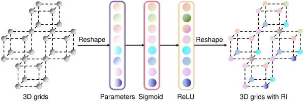
Figure 5: Structure of explicit representation and neural field. a, Initial 3D grids, depicting interconnected nodes arranged in a spatial structure. b, Reshape the 3D grids and set them as the parameters of the neural field. c, Processing through parameter layers followed by a sigmoid and ReLU function, which maps input values into a range between 0 and 1. d, Further reshaping the RI for multi-slice model.

Initially, we define a sparse voxel grid corresponding to the region of interest in the biological sample. Each voxel is then initialized as the parameters of the network using the Xavier method. This explicit method can easily be combined with other operations, such as a coarse-to-fine modeling, allowing direct upsampling or downsampling of the grid.

Our approach does not incorporate traditional neural network layers like linear or convolutional layers, significantly enhancing the model’s speed. To prevent large or negative values, we apply a combination of sigmoid and ReLU activation functions to the parameters:

$$\text{Out}=\text{ReLU}(\text{Sigmoid}(x)-0.5)$$ (6)

After this transformation, we reshape the parameters back into the grid format and then input them into our differential multi-slice model.

Data availability

The data used for reproducing the results in the manuscript are available at DFT website

Code availability

The code used for reproducing the results in the manuscript is available at DFT website

Contributions

The project was conceived by Y.X., and R.H.. The code of the model was implemented by R.H.. The experiments were designed by R.H., Y.C., and Y.X.. The numerical results were collected by R.H.. The 3D MuSCs tube was cultured by J.C.. The data acquisition and preparation was conducted by Y.C. and R.H.. The manuscript was primarily drafted by R.H.. and revised by Y.X., and reviewed by all authors.

Competing interests

The authors declare no competing interests.

References

- \bibcommenthead
- Xue et al. [2022] Xue, Y., Ren, D., Waller, L.: Three-dimensional bi-functional refractive index and fluorescence microscopy (brief). Biomed. Opt. Express 13(11), 5900–5908 (2022) https://doi.org/10.1364/BOE.456621
- Li and Xue [2024] Li, Y., Xue, Y.: Two-photon bi-functional refractive Index and fluorescence microscopy (2P-BRIEF). In: Brown, T.G., Wilson, T., Waller, L. (eds.) Three-Dimensional and Multidimensional Microscopy: Image Acquisition and Processing XXXI, vol. PC12848, p. 128480. SPIE, ??? (2024). https://doi.org/%****␣FDT.bbl␣Line␣75␣****10.1117/12.3001958 . International Society for Optics and Photonics. https://doi.org/10.1117/12.3001958
- Park et al. [2006] Park, Y., Popescu, G., Badizadegan, K., Dasari, R.R., Feld, M.S.: Diffraction phase and fluorescence microscopy. Opt. Express 14(18), 8263–8268 (2006) https://doi.org/10.1364/OE.14.008263
- Kim et al. [2017] Kim, K., Park, W.S., Na, S., Kim, S., Kim, T., Heo, W.D., Park, Y.: Correlative three-dimensional fluorescence and refractive index tomography: bridging the gap between molecular specificity and quantitative bioimaging. Biomed. Opt. Express 8(12), 5688–5697 (2017) https://doi.org/10.1364/BOE.8.005688
- Chowdhury et al. [2017] Chowdhury, S., Eldridge, W.J., Wax, A., Izatt, J.A.: Structured illumination multimodal 3d-resolved quantitative phase and fluorescence sub-diffraction microscopy. Biomed. Opt. Express 8(5), 2496–2518 (2017) https://doi.org/10.1364/BOE.8.002496
- Yeh et al. [2019] Yeh, L.-H., Chowdhury, S., Waller, L.: Computational structured illumination for high-content fluorescence and phase microscopy. Biomed. Opt. Express 10(4), 1978–1998 (2019) https://doi.org/10.1364/BOE.10.001978
- Choi et al. [2007] Choi, W., Fang-Yen, C., Badizadegan, K., Oh, S., Lue, N., Dasari, R.R., Feld, M.S.: Tomographic phase microscopy. Nat. Methods 4(9), 717–719 (2007)
- Sung et al. [2009] Sung, Y., Choi, W., Fang-Yen, C., Badizadegan, K., Dasari, R.R., Feld, M.S.: Optical diffraction tomography for high resolution live cell imaging. Opt. Express 17(1), 266–277 (2009) https://doi.org/10.1364/OE.17.000266
- Tian and Waller [2015] Tian, L., Waller, L.: Quantitative differential phase contrast imaging in an led array microscope. Opt. Express 23(9), 11394–11403 (2015) https://doi.org/10.1364/OE.23.011394
- Hugonnet et al. [2021] Hugonnet, H., Lee, M., Park, Y.: Optimizing illumination in three-dimensional deconvolution microscopy for accurate refractive index tomography. Opt. Express 29(5), 6293–6301 (2021) https://doi.org/10.1364/OE.412510
- Stockton et al. [2020] Stockton, P.A., Field, J.J., Squier, J., Pezeshki, A., Bartels, R.A.: Single-pixel fluorescent diffraction tomography. Optica 7(11), 1617–1620 (2020) https://doi.org/10.1364/OPTICA.400547
- an Pham et al. [2021] Pham, T.-a., Soubies, E., Soulez, F., Unser, M.: Optical diffraction tomography from single-molecule localization microscopy. Optics Communications 499, 127290 (2021) https://doi.org/10.1016/j.optcom.2021.127290
- Wang et al. [2024] Wang, K., Song, L., Wang, C., Ren, Z., Zhao, G., Dou, J., Di, J., Barbastathis, G., Zhou, R., Zhao, J., et al.: On the use of deep learning for phase recovery. Light: Science & Applications 13(1), 4 (2024)
- Dong et al. [2023] Dong, J., Valzania, L., Maillard, A., Pham, T.-a., Gigan, S., Unser, M.: Phase retrieval: From computational imaging to machine learning: A tutorial. IEEE Signal Processing Magazine 40(1), 45–57 (2023) https://doi.org/10.1109/MSP.2022.3219240
- Kamilov et al. [2015] Kamilov, U.S., Papadopoulos, I.N., Shoreh, M.H., Goy, A., Vonesch, C., Unser, M., Psaltis, D.: Learning approach to optical tomography. Optica 2(6), 517–522 (2015) https://doi.org/%****␣FDT.bbl␣Line␣300␣****10.1364/OPTICA.2.000517
- Jin et al. [2017] Jin, K.H., McCann, M.T., Froustey, E., Unser, M.: Deep convolutional neural network for inverse problems in imaging. IEEE transactions on image processing 26(9), 4509–4522 (2017)
- Wu et al. [2022] Wu, X., Wu, Z., Shanmugavel, S.C., Yu, H.Z., Zhu, Y.: Physics-informed neural network for phase imaging based on transport of intensity equation. Opt. Express 30(24), 43398–43416 (2022) https://doi.org/10.1364/OE.462844
- Rzepecki et al. [2022] Rzepecki, J., Bates, D., Doran, C.: Fast neural network based solving of partial differential equations. arXiv preprint arXiv:2205.08978 (2022)
- Liu et al. [2022] Liu, R., Sun, Y., Zhu, J., Tian, L., Kamilov, U.S.: Recovery of continuous 3d refractive index maps from discrete intensity-only measurements using neural fields. Nature Machine Intelligence 4(9), 781–791 (2022)
- Zhou et al. [2023] Zhou, H., Feng, B.Y., Guo, H., Lin, S.S., Liang, M., Metzler, C.A., Yang, C.: Fourier ptychographic microscopy image stack reconstruction using implicit neural representations. Optica 10(12), 1679–1687 (2023) https://doi.org/10.1364/OPTICA.505283
- Dwivedi et al. [2021] Dwivedi, V., Parashar, N., Srinivasan, B.: Distributed learning machines for solving forward and inverse problems in partial differential equations. Neurocomputing 420, 299–316 (2021) https://doi.org/10.1016/j.neucom.2020.09.006
- Chen et al. [2020] Chen, M., Ren, D., Liu, H.-Y., Chowdhury, S., Waller, L.: Multi-layer born multiple-scattering model for 3d phase microscopy. Optica 7(5), 394–403 (2020) https://doi.org/10.1364/OPTICA.383030
- Cao et al. [2022] Cao, R., Kellman, M., Ren, D., Eckert, R., Waller, L.: Self-calibrated 3d differential phase contrast microscopy with optimized illumination. Biomed. Opt. Express 13(3), 1671–1684 (2022) https://doi.org/10.1364/BOE.450838
- Chowdhury et al. [2019] Chowdhury, S., Chen, M., Eckert, R., Ren, D., Wu, F., Repina, N., Waller, L.: High-resolution 3d refractive index microscopy of multiple-scattering samples from intensity images. Optica 6(9), 1211–1219 (2019) https://doi.org/10.1364/OPTICA.6.001211
- Yu et al. [2021] Yu, A., Li, R., Tancik, M., Li, H., Ng, R., Kanazawa, A.: Plenoctrees for real-time rendering of neural radiance fields. In: Proceedings of the IEEE/CVF International Conference on Computer Vision, pp. 5752–5761 (2021)
- Li et al. [2011] Li, J., Gonzalez, J., Walker, D., Hersom, M., Ealy, A., Johnson, S.: Evidence of heterogeneity within bovine satellite cells isolated from young and adult animals. Journal of animal science 89, 1751–7 (2011) https://doi.org/10.2527/jas.2010-3568
- Fridovich-Keil et al. [2022] Fridovich-Keil, S., Yu, A., Tancik, M., Chen, Q., Recht, B., Kanazawa, A.: Plenoxels: Radiance fields without neural networks. In: 2022 IEEE/CVF Conference on Computer Vision and Pattern Recognition (CVPR), pp. 5491–5500 (2022). https://doi.org/10.1109/CVPR52688.2022.00542