Magnetic Fields in Massive Star-forming Regions (MagMaR): Unveiling an Hourglass Magnetic Field in G333.46$-$0.16 using ALMA

Abstract

The contribution of the magnetic field to the formation of high-mass stars is poorly understood. We report the high-angular resolution ($\sim 0.3^{\prime\prime}$, 870 au) map of the magnetic field projected on the plane of the sky (B_pos) towards the high-mass star forming region G333.46$-$0.16 (G333), obtained with the Atacama Large Millimeter/submillimeter Array (ALMA) at 1.2 mm as part of the Magnetic Fields in Massive Star-forming Regions (MagMaR) survey. The B_pos morphology found in this region is consistent with a canonical “hourglass” which suggest a dynamically important field. This region is fragmented into two protostars separated by $\sim 1740$ au. Interestingly, by analysing H¹³CO⁺ ($J=3-2$) line emission, we find no velocity gradient over the extend of the continuum which is consistent with a strong field. We model the B_pos, obtaining a marginally supercritical mass-to-flux ratio of 1.43, suggesting a initially strongly magnetized environment. Based on the Davis–Chandrasekhar–Fermi method, the magnetic field strength towards G333 is estimated to be $5.7$ mG. The absence of strong rotation and outflows towards the central region of G333 suggests strong magnetic braking, consistent with a highly magnetized environment. Our study shows that despite being a strong regulator, the magnetic energy fails to prevent the process of fragmentation, as revealed by the formation of the two protostars in the central region.

1 Introduction

Star formation is a complex process controlled by several factors, among which gravity, turbulence, and magnetic field play a key role. Magnetic fields are believed to oppose the gravitational contraction and fragmentation of dense cores, thus delaying the formation of protostars (e.g., Mouschovias & Ciolek, 1999; McKee & Ostriker, 2007; Li et al., 2017; Palau et al., 2021; Hwang et al., 2022). However, magnetic fields can also help to channel cloud material towards overdense regions, thus acting as a catalyst in the formation of protostars (e.g., Soler & Hennebelle, 2017; Hennebelle & Inutsuka, 2019).

In a strongly magnetic environment, the morphology of the magnetic field remains preserved up to scales of dense molecular cores of $0.01-0.1$ pc (e.g., Qiu et al., 2014; Li et al., 2015; Cortés et al., 2021). Another possible scenario shows the dragging of the frozen-in magnetic field along with the gas material towards the dense core by the gravitational collapse. This phenomenon creates a pinching effect in the magnetic field lines, leading to an “hourglass”-like appearance (e.g., Girart et al., 2006, 2009; Rao et al., 2009; Tang et al., 2009; Stephens et al., 2013; Hull et al., 2014; Qiu et al., 2014; Maury et al., 2018; Koch et al., 2018; Beltrán et al., 2019; Kwon et al., 2019; Cortés et al., 2021; Huang et al., 2024). This specific structure may be partially due to projection and line-of-sight integration effects that lead to the observed dust polarization. It is of utmost importance to characterize hourglass patterns when observed, in order to better understand the initial conditions of star formation.

Despite being a significant regulator of star formation, the role of the magnetic field during the birth of massive stars is still poorly understood. To make progress, a survey Magnetic fields in Massive star-forming Regions (MagMaR) has been carried out. In MagMaR, a total of 30 high-mass star-forming regions were observed at 1.2 mm with the Atacama Large Millimeter/ submillimeter Array (ALMA). A few detailed characteristics of some targets, such as G5.89$-$0.39, IRAS 18089$-$1732, and NGC 6334I(N), have been discussed by Fernández-López et al. (2021), Sanhueza et al. (2021), and Cortés et al. (2021), respectively.

Out of the 30 targets, the magnetic field projected on the plane of the sky (B_POS) towards the high-mass star-forming region G333.46$-$0.16 (hereafter, G333) shows the most extended hourglass morphology on a few 1000 au scale (assuming a distance of 2.9 kpc; Lin et al., 2019). This target was studied as a part of the ATLASGAL survey of massive clumps by Csengeri et al. (2014) and Lin et al. (2019). The bolometric luminosity of this target is of 4.4$\times$10³ L_⊙ (Lin et al., 2019). Based on its spectral energy distribution, Lin et al. (2019) estimated a dust temperature and mass of 25.2 K and 282 M_⊙, respectively for this region. Here, we aim to assess magnetic properties and to investigate the importance of the magnetic field, gravity and turbulence in the star-forming region G333.

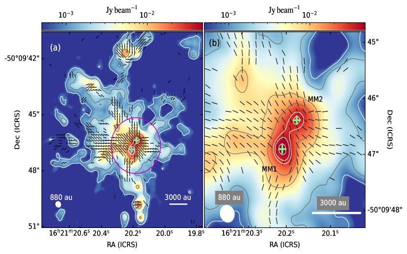
Figure 1: (a) The B_POS geometry (black line segments) towards G333, obtained after rotating the polarization segments by 90^∘, overplotted on ALMA 1.2 mm dust continuum emission. The B_POS segments have arbitrary length and plotted above the 3$\sigma$ ($\sigma=29\mu$Jy beam^-1 for Stokes $Q$ and $U$) level. Contours correspond to dust continuum emission 5, 10, 50, 100, 190, 230, 300 and 340 times $\sigma$ ($=160\mu$Jy beam^-1). The positions of MM1 and MM2 are marked as ‘+’ symbols. The circle in magenta represents the area of analysis. The scale bar and the beamsize of 880 au are displayed on the bottom right and bottom left sides, respectively. The line segments are drawn following the Nyquist sampling (every three pixels each of size $0.05^{\prime\prime}$). (b) Magnified view of the area of analysis. Symbols are the same as in panel (a).

2 Observations

ALMA polarimetric observations towards G333 were carried out on 2018 September 27 using ALMA Band 6 (1.2 mm) as a part of the MagMaR project (Project ID: 2017.1.00101.S and 2018.1.00105.S; PI: P. Sanhueza). The maximum recoverable scale (MRS) was $\sim 4.5^{\prime\prime}$. During the observing runs, J1650-5044 was used as phase calibrator while J1427-4206 was used as a calibrator for bandpass, flux, and polarization. Details of the observational setup are discussed by Fernández-López et al. (2021), Sanhueza et al. (2021), and Cortés et al. (2021).

Linearly polarized dust continuum emission is identified within the the inner one-third area of the primary beam (24^′′). Bright emission lines have been eliminated from the Stokes $I$ continuum following the method elaborated by Olguin et al. (2021). We used CASA 6.5.2 to perform self-calibration and imaging. Self-calibration of the Stokes $I$ was performed with three iterations in phase with a final solution interval of 10 seconds. The self-calibration solutions were applied to the respective spectral cubes. The imaging of each Stokes parameter was performed separately employing the CASA task tclean using Briggs weighting with a robust parameter of 1. The resulting Stokes $I$ image has an angular resolution of 0.318${}^{\prime\prime}\times 0.290^{\prime\prime}$ with a position angle of 49.4^∘ (922$\times$841 au). The sensitivities of the images are 160 $\mu$Jy beam^-1 for the final Stokes $I$, and 29 $\mu$Jy beam^-1 for the final Stokes $Q$, and $U$. The source is bright in continuum Stokes $I$ emission making the image dynamic range limited. However, the polarized emission (Stokes $Q$ and $U$) is significantly weaker compared to the continuum Stokes $I$ and therefore, it is unlikely to be dynamic range limited, making them possible to reach the thermal noise. The debiased linear polarized intensity, polarization fraction and polarization angle images were constructed following Vaillancourt (2006).

The image of H¹³CO${}^{+}(J=3-2)$ line emission, also included in the spectral setup, was obtained by the automatic masking method yclean (Contreras et al., 2018). The CASA task tclean was performed using Briggs weighting with a robust parameter of 1, leading to a noise level of 2.9 mJy beam^-1 (0.61 K) per 0.56 km s^-1 channel.

3 Results

The ALMA 1.2 mm continuum emission with $\sim 900$ au spatial resolution is shown in Figure 1 a and reveals details of the internal structure of G333. The dust continuum emission shows a flattened structure that is elongated in the northwest-southeast direction. The center of this flattened structure is fragmented into two more condensations with a separation of $\sim 1740$ au along the major axis of the elongation. Both the condensations show presence of hot molecular core emission lines (Taniguchi et al., 2023), suggesting that they are potential protostars. The peak flux at the position of the brightest component, located towards the south-east (MM1), is $53.5$ mJy beam^-1, while the fainter one located towards the north-west (MM2) has a peak flux of $38.8$ mJy beam^-1.

The direction of the B_pos  is inferred by assuming the dust grains are aligned with respect to the magnetic fields (i.e., rotating the polarization segments by $90^{\circ}$; Cudlip et al., 1982; Hildebrand et al., 1984; Hildebrand, 1988; Lazarian, 2000; Andersson et al., 2015). The polarized emission detected in G333 suggests an hourglass-like geometry of the magnetic field aligned with the symmetry axis of the hourglass almost parallel to the minor axis of the flattened envelope. For our analysis, we focus on the circular area as marked in Figure 1 (a), that harbours the hourglass magnetic field. We chose this area to avoid the additional distortion of B_pos produced by other surrounding cores. The circle is centered at $\alpha=16:21:20.183$ and $\delta=-50:09:46.662$, with a radius of $1.5^{\prime\prime}$ (4350 au). As the diameter of the area of analysis ($3^{\prime\prime}$) is less than the MRS, the extended emission should not be significantly affected by filtering.

Being a cold dense gas tracer (upper energy level, $E_{u}$ of 25 K), the spatial distribution of H¹³CO${}^{+}(J=3-2)$ line emission towards G333 appears to be similar to that of the dust continuum emission (see Figure 2 a). Figure 2 (b) shows the H¹³CO⁺ distribution of the intensity-weighted velocity structure (moment 1 map) towards G333 with respect to the systemic velocity ($v_{\mathrm{lsr}}\sim-43$ km s^-1). No clear signature of large-scale velocity gradient is detected with a spectral resolution of 0.56 km s^-1, suggesting a quiescent environment at $\sim 10000$ au scale. However, the velocity field over MM1 and MM2 is relatively more blueshifted than their immediate vicinities, which could be a sign of infall as suggested by Estalella et al. (2019) and Olguin et al. (2021).

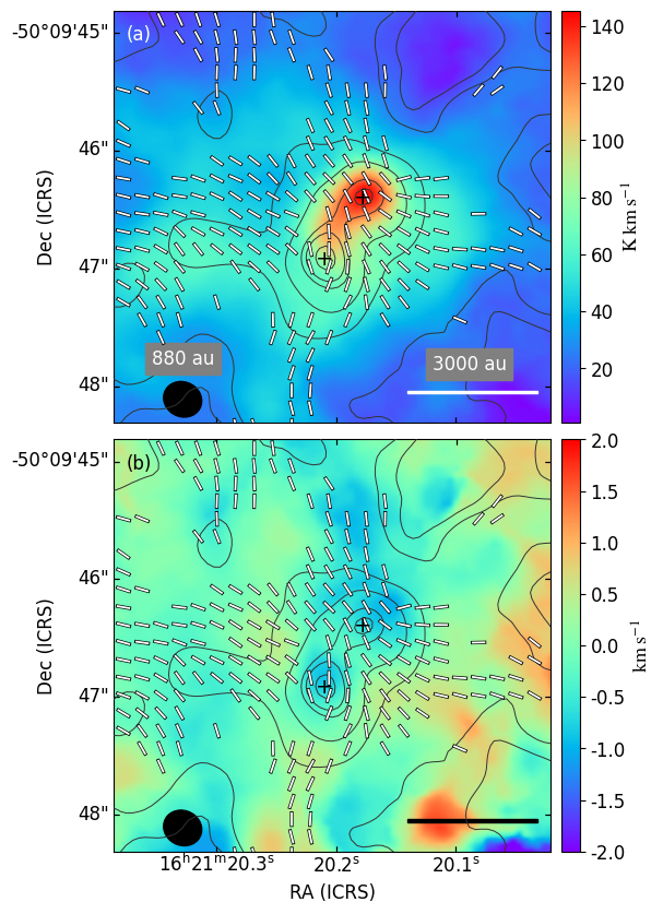
Figure 2: (a) The moment 0 or integrated intensity map of H¹³CO⁺ line emission. (b) The moment 1 or intensity weighted velocity map of the same. The white line segments show the B_POS geometry and the contours outline the dust continuum emission (same as Figure 1). The positions of MM1 and MM2 are marked as ‘+’ symbols. The scale bar and the spatial resolution are displayed on the bottom right and bottom left sides, respectively, in all panels.

4 Discussion

4.1 Dust continuum emission and velocity dispersion

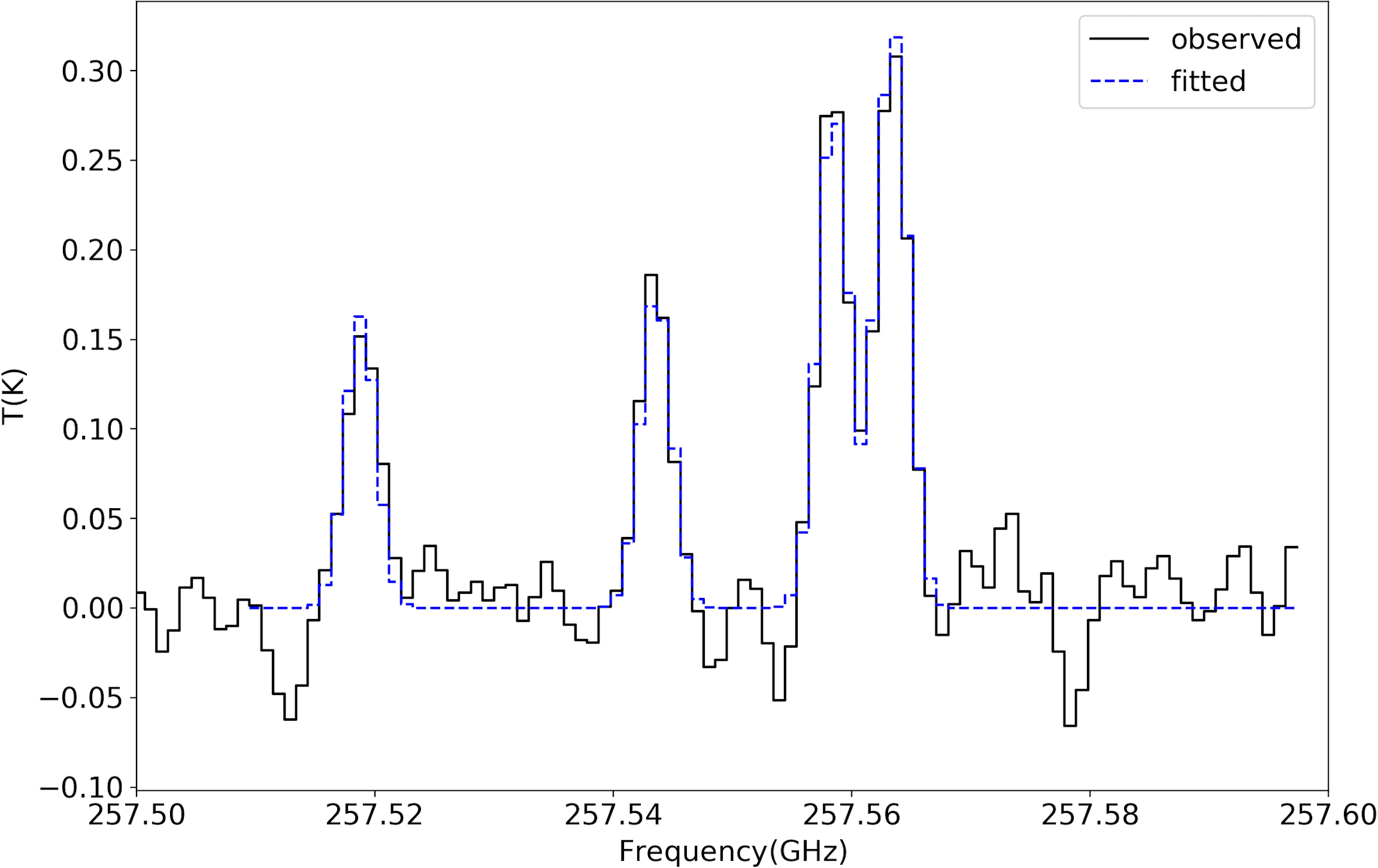
Figure 4: The spectra of CH₃CN ($J=14-13$) towards G333. The black line shows the observed spectrum and the dashed blue line shows the fitted spectrum.

The flux density enclosed in the circular region is 493 mJy. The temperature of the region marked with a circle as in Figure 1, is determined using the CH₃CN ($J=14-13$) rotational transitions. We detected primarily 4 brightest K components (K = 0, 1, 2, 3) of the transition towards this area. We avoided the region very close to MM1 and MM2 to refrain the line contamination by radiation from MM1 and MM2. In Figure 4, we present the average brightness distribution of the CH₃CN ($J=14-13$) transitions in black. The blue dashed line represents the fitted spectrum that is obtained by fitting the observed spectrum with XCLASS (Möller et al., 2017) resulting in a temperature of 50 K. Using this temperature, and assuming optically thin dust emission and a spherical geometry, the total gas mass is estimated using:

$$M=\Lambda\frac{F_{\nu}D^{2}}{\kappa_{\nu}B_{\nu}(T)}$$ (1)

where $\Lambda$ is the gas-to-dust mass ratio, $F_{\nu}$ is the flux density of the source, $D$ is the distance to the target, $\kappa_{\nu}$ is the dust opacity per gram of dust, and $B_{\nu}$ is the Planck function with a dust temperature T. The gas-to-dust ratio is assumed to be 100:1. The dust opacity is assumed as 1.03 cm²g^-1 (interpolated to 1.2 mm; Ossenkopf & Henning, 1994). Using a dust temperature of 50 K, the total mass is estimated as 23 M_⊙.

We estimate the mass density $\rho$ as $3.9\times 10^{-17}$ gm cm^-3, using a volume ($V=\frac{4}{3}\pi R^{3}$, where, $R=1.5^{\prime\prime}$). The number density $n(\rm H_{2})$ is $\rho/\mu_{\rm H_{2}}m_{\rm H}$, where $\mu_{\rm H_{2}}(=2.86)$ is the mean molecular weight per hydrogen molecule (Kirk et al., 2013) and $m_{\rm H}$ is the atomic mass of hydrogen. The $n(\rm H_{2})$ enclosed in the area of analysis is estimated as $8.4\times 10^{6}$ cm^-3.

Using the dendogram technique (Rosolowsky et al., 2008) adopted in the astrodendro Python package , the flux densities of MM1 and MM2 are estimated as 59.5 mJy and 25.8 mJy, respectively. Assuming the similar temperature, MM1 is 2.3 times more massive than MM2. Table 1 lists the dendogram results for both protostars.

Considering a bolometric luminosity of $4.4\times 10^{3}$ L_⊙ (Lin et al., 2019), and assuming that a single main-sequence star is responsible for the bolometric luminosity, the stellar mass would then be $\sim 6$ M_⊙ (Mottram et al., 2011). However, there are two protostars at the center. At larger scale, based on the ALMA 7m array observations with an angular resolution of $3.7^{\prime\prime}$ (Csengeri et al., 2017), the mass of the structure containing MM1 and MM2 is determined as 120 M_⊙, suggesting that most of the clump mass (282 M_⊙) is concentrated in the central region of the clump. Thus, these protostars are potential candidates to becoming high-mass stars by accreting gas material from the available mass reservoir.

Using H¹³CO⁺ line emission, we derive the dispersion in the turbulent velocity along the line of sight, $\sigma v_{\mathrm{los}}(=\sqrt{\sigma_{\rm obs}^{2}-\sigma_{th}^{2}})$. The $\sigma_{\rm obs}$ and $\sigma_{th}$ are the total observed and thermal velocity dispersions, respectively. The $\sigma_{th}$ can be expressed as $\sqrt{k_{B}T/\mu m_{\rm H}}$, where $k_{B}$ is the Boltzmann constant, $\mu$ is the mean molecular weight per free particle (30). Assuming a temperature of 50 K, $\sigma_{th}$ and $\sigma v_{\mathrm{los}}$ are estimated as 0.12 and 1.21 km s^-1, respectively.

4.2 Modeling of the hourglass-shaped magnetic field

In order to model the magnetic field pattern, we used the DustPol module included in the ARTIST package (Padovani et al., 2012), which is based on the Line Modeling Engine (LIME) radiative transfer code (Brinch & Hogerheijde, 2010). DustPol generates the synthetic Stokes $I$, $Q$, and $U$ images in FITS-format, which are used as an input for the simobserve and simanalyze tasks of CASA, considering the same antenna configuration of the observing runs in ALMA. In this way, polarization position angle maps are created and compared with the observations. The physical modeling of the 3D magnetic field is done by combining an axisymmetric singular toroid threaded by a poloidal field (Li & Shu, 1996; Padovani & Galli, 2011). Based on Padovani et al. (2013), we added a toroidal force-free component of the magnetic field to represent the effects of rotation.

The model used in this work has four free parameters: (1) the mass-to-flux ratio normalized to its critical value, $\lambda$, defined as,

$$\lambda=\frac{(M/\Phi_{B})}{(M/\Phi_{B})_{cr}}=2\pi\sqrt{G}\frac{M}{\Phi_{B}}$$ (2)

where $G$ is the gravitational constant, $\Phi_{B}$ is the magnetic flux ($=\pi R^{2}B$), and $M$ is the mass of the core; (2) the ratio of the strengths of the toroidal and the poloidal components of the magnetic field in the midplane of the source, $b_{0}$; (3) the orientation of the magnetic axis projected on the plane of sky, $\varphi$, starting from north and increasing eastward; (4) the inclination with respect to the plane of the sky, $i$, with an assumption to be positive/negative when the magnetic field in the northern part directs towards/away from us. A $\chi^{2}$-test is performed on the polarization angle residuals $(\Delta\psi)$ of the polarization angle $\psi$, obtained from the difference between the observed ($\psi_{\rm obs}$) and the modeled ($\psi_{\rm mod}$) polarization angles ($\Delta\psi=\psi_{\rm obs}-\psi_{\rm mod}$), enclosed within the circular area for each combination of the four free parameters. The $\chi^{2}$ is estimated accounting for regions lying above the 3$\sigma$ level ($\sigma=29\mu$Jy beam^-1) of Stokes $Q$ and $U$ images. A constant temperature (50 K) has been adopted in the modelling as no temperature map of this region is available currently. On the other way, the region close to MM1 and MM2, is expected to be relatively hot and having more weight in estimating the Stokes parameters.

The best-fit model provides the minimum reduced $\chi^{2}$ value of 9.39 with the combination of model parameters: $\lambda=1.63$, $b_{0}=-0.1\pm 0.1$, $i=45^{\circ+13^{\circ}}_{-6^{\circ}}$, and $\varphi=40^{\circ+1^{\circ}}_{-4^{\circ}}$. The errors are estimated following Lampton et al. (1976). A low value of $b_{0}$ in the best-fit model is consistent with no apparent rotation towards G333 as found in H¹³CO⁺. The value of $\lambda=1.63$ obtained from the model (see Equation 2) is relative to the mass enclosed in a flux tube, but observationally the mass is derived considering a spherical system. Therefore, the estimated $\lambda$ is transformed to an effective $\lambda$ of 1.43 (Li & Shu, 1996), which is marginally supercritical.

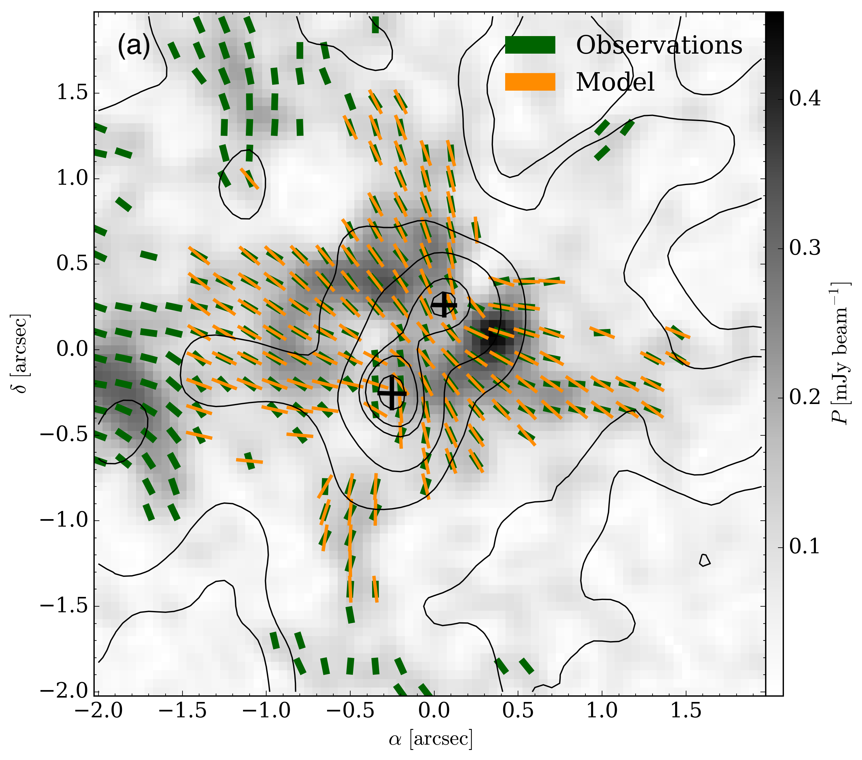
Figure 3: (a) Comparison between the observed (green segments) and modeled (yellow segments) magnetic field orientations overplotted on the polarized intensity map (grayscale). The black contours are the same as Figure 1. (b) Histogram of the polarization angle residuals ($\Delta\psi$) along with the Gaussian fitting.

In Figure 3 (a), we show a comparison between the observed and modeled magnetic field geometry, limited to the area within the circle shown in Figure 1 (a). Although the hourglass model reproduces quite well the observed magnetic field geometry, deviations can be seen around MM1, mainly towards its southern and eastern regions. Since MM1 is relatively more massive than MM2, it is possible that the gravity of MM1 might have dragged and distorted the magnetic field lines more effectively than MM2. In Figure 3 (b), we show the histogram of the $\Delta\psi$. A Gaussian fit to the whole distribution of $\Delta\psi$ provides a mean value $\textless\Delta\psi\textgreater=-3.32^{\circ}$ and a standard deviation $\sigma_{\psi}=19.48^{\circ}$.

4.3 Magnetic field strength

We estimate B_POS towards G333 using the well-known Davis–Chandrasekhar–Fermi (DCF) method (Davis, 1951; Chandrasekhar & Fermi, 1953), which states:

$$B_{\mathrm{POS}}=Q\sqrt{4\pi\rho}\frac{\sigma v_{\mathrm{los}}}{\delta\psi_{int}}$$ (3)

where Q is a correction factor, 0.5, adopted from simulations in turbulent clouds (Ostriker et al., 2001), $\rho$ is the mass density of the cloud, $\sigma v_{\mathrm{los}}$ is the dispersion in the turbulent velocity along the line of sight, and $\delta\psi_{int}$ is the intrinsic dispersion in the polarization angle $\psi$. The $\delta\psi_{int}$ can be obtained from $\sqrt{\sigma_{\psi}^{2}-\delta\psi_{\rm obs}^{2}}$. The average uncertainty in the observed $\psi$ within the circle of analysis is $\delta\psi_{\rm obs}=5.4^{\circ}$. The $\delta\psi_{int}$ obtained is $18.7^{\circ}$. Consequently, $B_{\mathrm{pos}}$ is estimated as 4.0 mG. Adopting $i=45^{\circ}$ from our model, we also estimate the total magnetic field strength $B=B_{\mathrm{pos}}/\mathrm{cos}~{}(i)=5.7$ mG. With a density of n(H${}_{2})=8.4\times 10^{6}$ cm^-3 this strength is consistent as found in the compilation of B-field strength with density by Liu et al. (2022a) using the DCF method.

The DCF method assumes the deviation of uniform magnetic field by turbulent gas motions, without considering gravity, which is most likely responsible for the hourglass shape. In this work gravity is taken into account while using the dustPol model and by considering the $\Delta\psi$, we eliminate the gravitational effect and the $\delta\psi$ is supposed to be the interplay between the turbulence and the magnetic field.

While computing $\lambda$ using Equation 2, we assumed that all the mass is in the envelope, while the protostellar mass should also be added to the envelope mass. Therefore, the estimated $\lambda$ should be considered as a lower limit. As mentioned in 4.1, based on the luminosity, an additional stellar mass of $\sim 6$ M_⊙ could be added to the envelope mass, making the total mass of 29 M_⊙, which leads to a mass-to-flux ratio of 1.22. The fact that the dust emission may be optically thick at the very central bright fragmented region, leads to underestimate the mass of the circular region can not be ignored. However, the estimated value of $\lambda$ is similar to the one obtained from the modelling (1.43).

We compute the Alfv$\mathrm{\acute{e}}$n speed $v_{\rm A}=B/\sqrt{4\pi\rho}=2.58$ km s^-1, through which we estimate the turbulent to magnetic energy $\beta_{t}=3(\sigma v_{\mathrm{los}}/v_{\rm A})^{2}=0.66$. This indicates that the magnetic energy dominates moderately over the turbulent energy in this region. Thus the magnetic field towards G333, in spite of being quite strong, could not prevent the fragmentation and eventually star formation.

Based on a non-ideal magnetohydrodynamic simulations of an initially subcritical core by Machida & Basu (2020), the collapse happens after the core reaches a marginally supercritical mass-to-flux ratio, leaving behind a considerable amount of magnetic flux, which helps to transport out the angular momentum through strong magnetic braking. As a result, the protostar may harbour no disc or a very small one, with a very weak outflow signature. In G333, we do not find any evidence of rotation in the envelope region (Figure 2 b), nor in any of the protostars at the current angular resolution. Even in higher angular resolution ($\sim 0.05^{"}$) observations of the same region obtained as part of the Digging into the Interior of Hot Cores with the ALMA (DIHCA; Olguin et al., 2022, 2023; Taniguchi et al., 2023) survey (P. Sanhueza, private communication), no clear signature of rotation was found in any of the protostars, making the argument of strong magnetic braking more evident. Additionally, we found no significant outflow signature coming from the two protostars in G333 (see appendix A). This is consistent with overall physical scenario of very weak outflow and no disk when starting with strongly magnetized initial conditions (Machida & Basu, 2020). This leads to the possibility that star formation in G333 started in an initially subcritical or transcritical cloud.

4.4 Analysis of the Energy Balance

The current dynamical state towards G333 can be inferred from the virial parameter ($\alpha_{\mathrm{vir}}$), the ratio of the virial mass ($M_{\mathrm{vir}}$) to the total mass ($M$) of the system with considerations of both the turbulent and magnetic supports. While $\alpha_{\mathrm{vir}}\sim 1$ indicates the equilibrium state, $\alpha_{\mathrm{vir}}\textgreater 1$ implies expansion and conversely $\alpha_{\mathrm{vir}}\textless 1$ signifies contraction under gravity. We estimate $\alpha_{\mathrm{vir}}$ as $1.3$ for a centrally peaked density profile (see Appendix B). This suggests that G333 is currently close to a quasi-equilibrium state or undergoing quasi-static evolution, which is further supported by the quiescent environment of G333 as implied by the velocity field traced by the H¹³CO⁺ line emission (Figure 2 b). A strongly magnetized environment exerts an adequate support against rapid gravitational collapse, although the magnetic field could not hinder the fragmentation. This is consistent with a second stage of fragmentation within an initial massive core that forms out of a transcritical cloud (Bailey & Basu, 2014).

4.5 Flattened envelope harbouring the hourglass magnetic field

Theoretical studies suggests that for a relatively strong magnetic field environment ($\lambda\leq 3$), the core material is channeled primarily along the magnetic field lines by the gravitational pull, building a flattened pancake-like structure perpendicular to the field lines, and developing a small toroidal component of the magnetic field (Allen et al., 2003; Price & Bate, 2007). As shown in Figure 1, the flattened structure where the fragmentation took place agrees well with the strong magnetic field case, which is further supported by a low $\lambda$ obtained from our best-fit model as well as the observations. Additionally a small contribution of the toroidal component of the field ($\sim 10\%$ of the poloidal component) obtained from the best-fit model supports this phenomenon. This is consistent with some previous studies (e.g., Qiu et al., 2014; Beltrán et al., 2019; Kwon et al., 2019), which suggest a major contribution of magnetic field in the formation of high-mass protostars.

4.6 Stability analysis of the central protostars

To investigate whether the central protostars MM1 and MM2 are gravitationally bound, we followed the methodology adopted in Pineda et al. (2015) and Li et al. (2024). We estimate the gravitational potential energy ($V_{i}$) by

$$V_{i}=-\sum_{i\neq j}\frac{Gm_{i}m_{j}}{r_{ij}}$$ (4)

where $m_{i}$ and $m_{j}$ are the masses of objects $i$ and $j$, respectively, and $r_{ij}$ is the separation between them. The kinetic energy ($E_{i}$) is given by,

$$E_{i}=\frac{1}{2}m_{i}(v_{i}-v_{com})^{2}$$ (5)

where $v_{i}$ is the line-of-sight velocity of the object $i$, and $v_{com}$ is the velocity of the centre of mass of the system. We estimate $v_{com}$ by

$$v_{com}=\frac{\sum_{k}{m_{k}v_{k}}}{\sum_{k}{m_{k}}}$$ (6)

The velocities of MM1 and MM2 are obtained from Taniguchi et al. (2023) as $-44.06$ and $-43.55$ km s^-1, respectively. Assuming that the measured velocity difference between MM1 and MM2 is in 1-D, the full velocity difference in 3-D is $\Delta v_{3D}=\sqrt{3}({v_{i}-v_{com}})$ along the line-of-sight. Also, the total separation between MM1 and MM2 is estimated by multiplying the measured projected separation (1740 au) with $4/\pi$, i.e., 2215 au, assuming a random orientation between them.

We measured the masses of MM1 and MM2 from the flux density obtained from the astrodendro task to estimate the $E_{i}/V_{i}$ for each of them. The $E_{i}/V_{i}$ for MM1 and MM2 are estimated as 0.08 and 0.17, respectively. As both MM1 and MM2 show $E_{i}/V_{i}\textless 1$, they could be gravitationally bound in a binary system at the present stage.

5 Summary and Conclusions

The ALMA high-angular resolution ($\sim 0.3^{\prime\prime}$) observations of linearly polarized 1.2 mm dust emission towards the high-mass star-forming region G333.46$-$0.16 revealed an hourglass-shaped pattern of B_pos at a scale of $\sim 6000$ au. The hourglass shape is found to be more pinched towards MM1 than MM2, which might be because of the larger mass of MM1 compared to MM2. The protostars MM1 and MM2 are found to be gravitationally bound in a binary system at present with a separation of $1740$ au.

The H¹³CO⁺ line emission shows no strong velocity gradient that could hint any rotation towards G333. Also, none of the protostars show any clear signature of outflows, suggesting a strong magnetic braking.

The hourglass-shaped B_pos  is well fitted with an axisymmetric semi-analytical magnetostatic model. The best fit model is primarily governed by a poloidal component tangled with a small toroidal component ($\sim 10\%$ of the poloidal one). The best fit results also provide $\lambda=1.43$, $i=45^{\circ+13^{\circ}}_{-6^{\circ}}$ and $\phi=40^{\circ+1^{\circ}}_{-4^{\circ}}$.

Based on the DCF relation, the total magnetic field strength is estimated as $5.7$ mG. We also estimate the mass-to-flux ratio using the dispersion of polarization angle obtained from the model fitting, which results in $1.22$, consistent with same obtained from the best fit model ($\lambda=1.43$).

Our analysis of energy balance in this area suggests a quasi-equilibrium state, which is consistent with the current dynamic environment inferred by H¹³CO⁺ line emission. Our speculation based on this work is that the magnetic field towards G333 is strong enough to stabilize the environment towards the center. A low magnitude of turbulent-to-magnetic energy ratio indicates a suppression of the magnetic field over the turbulence in this region. However, both are ultimately overwhelmed by the gravity, responsible for the fragmentation and eventually star formation. This leads to a possible scenario that the star formation in G333 might have started in an initially subcritical core, when the very central peak density area reached the marginally supercritical mass-to-flux ratio.

Table 1: Results obtained from astrodendro^∗

R.A.	Dec.	FWHM	Peak Intensity	Flux Density
(ICRS)	(ICRS)	$(^{\prime\prime}\times^{\prime\prime})$	(mJy beam-1)	(mJy)
MM1
16:21:20.20	-50:09:46.91	$0.31\times 0.21$	53.5	59.5
MM2
16:21:20.17	-50:09:46.41	$0.23\times 0.14$	38.8	25.8

^∗ $F_{min}=5\sigma$: the threshold above which the structures are defined.
$\delta=1\sigma$: the minimum significance for separation of the structures.
$S_{min}=$half of the beamsize: the minimum area to be allocated in the individual structure.

Appendix A Molecular outflows identified around G333

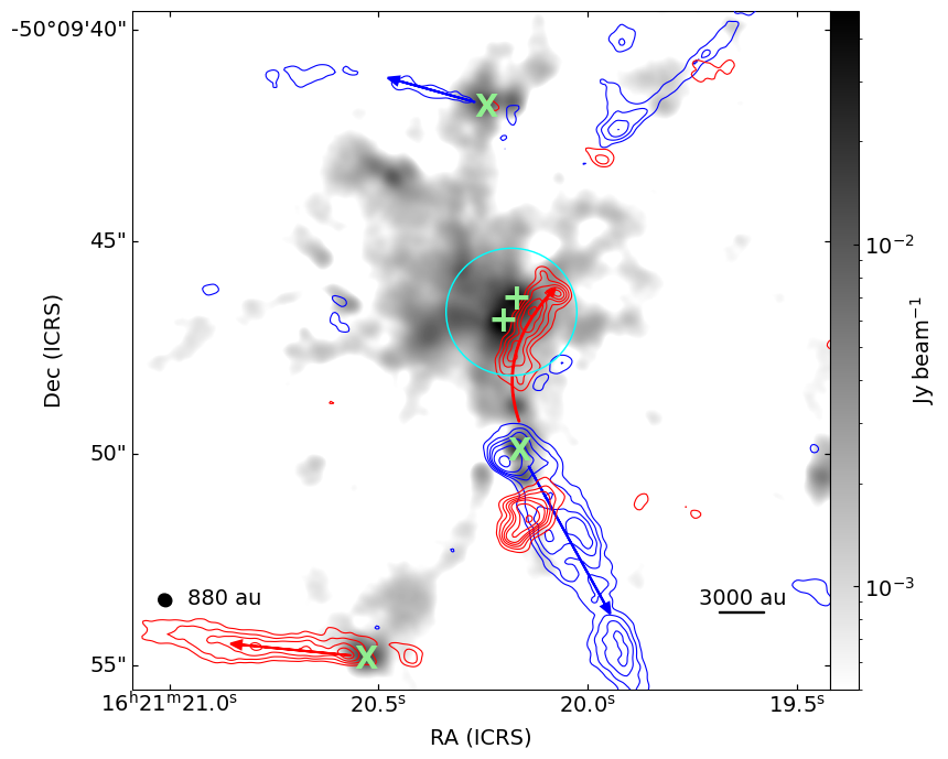
Figure 5: Molecular outflows identified in ¹²CO $(J=3-2)$ overplotted on our observed 1.2 mm dust continuum emission. The plus symbols mark the positions of MM1 and MM2. The circle in cyan shows the region of analysis. The blueshifted and redshifted outflows are shown in blue and red contours, respectively. The blue contours are drawn with levels 3,5,7,9,12, and 18 times 0.13 Jy beam^-1. The red contours are drawn with levels 3,5,7,9,11,15,20, and 25 times 0.10 Jy beam^-1. The possible sources driving the ouflows are marked using green ‘X’ symbols. The red and blue arrows show the directions of the redshifted and blueshifted outflows, respectively.

Several molecular outflows are identified around G333 using the ¹²CO ($J=3-2$) line emission observed by ALMA (Project ID: 2013.1.00960.S, PI: T. Csengeri). Using the CASA task imregrid, we match the phase-center of the ¹²CO line image and our 1.2 mm dust continuum image.

Figure 5 shows the ¹²CO molecular outflows overplotted on the dust continuum image. The ¹²CO line emission is integrated from $-106.1$ to $-65.3$ km s^-1 for the blueshifted lobe, and $-22.1$ to $0.7$ km s^-1 for the redshifted lobe. The sensitivities of the integrated images of the blueshifted and redshifted ¹²CO line emission are 0.14 and 0.10 Jy beam^-1, respectively. The outflow lobes in the north and south of the region enclosed by the hourglass-shaped magnetic field (shown as a cyan colored circle in Figure 5) are highly collimated. Interestingly, it is noticeable that although there is a significant amount of redshifted ¹²CO line emission within the circle (which seems to be the redshifted lobe of the nearby dense core located south to the circular area of analysis), none of the outflow lobes is driven by any of the protostars but likely the low-mass protostars residing outskirts of the dense gas. There are some dust condensations that likely could host these protostars, marked with ‘X’ symbols in Figure 5.

The absence of outflows in any of the protostars makes it difficult to predict the of angular momentum direction. In a classical scenario of magnetized star formation, the angular momentum is efficiently lost by magnetic braking (Mouschovias & Paleologou, 1979). Our speculation is that magnetic braking is relatively strong in the case of G333, because of which we do not find any observational signature of strong angular momentum.

Appendix B Virial parameter

The virial theorem can be expressed as below:

$$\frac{1}{2}\frac{d^{2}I}{dt^{2}}=2E_{k}+E_{G}+E_{B}$$ (B1)

where $I$ is the moment of inertia, $E_{k}$, $E_{G}$, and $E_{B}$ are the kinetic, gravitational, and magnetic energy, respectively. We consider a spherical cloud having a radial density profile $\rho\propto r^{-\alpha}$, where $\alpha=2$ imply the density profile to be centrally peaked (Belloche, 2013). The gravitational energy ($E_{G}$) can be expressed by:

$$E_{G}=-\frac{(3-\alpha)}{(5-2\alpha)}\frac{GM^{2}}{R}$$ (B2)

The magnetic energy ($E_{B}$) is given by:

$$E_{B}=\frac{B^{2}V}{8\pi}$$ (B3)

The kinetic energy ($E_{k}$) is derived by:

$$E_{k}=-\frac{3}{2}M\sigma_{\rm obs}^{2}$$ (B4)

The rotational energy ($E_{r}$) is expressed as:

$$E_{r}=\frac{1}{3}Mv_{\rm rot}^{2}\frac{(3-\alpha)}{(5-\alpha)}$$ (B5)

We do not find any evidence of rotation with a spectral resolution 0.56 km s^-1 in the area of analysis. If we assume this resolution as the upper limit of the velocity due to rotation ($v_{\rm rot}$), we estimate the ratio $E_{rot}/E_{G}$ to be 0.006 for a centrally peak density profile. With the same assumption of rotation, a ratio of $E_{rot}/E_{B}$ is estimated to be 0.013 for the same profile. Similarly, we estimate the ratio of $E_{rot}/E_{k}$ as 0.014. As the contribution of the rotational energy is negligible compared to the other energies, we do not account the upper limit of rotational term in the estimation of virial parameter.

Including both the kinetic and magnetic energies, a system can be in stable phase, when $2E_{k}+E_{B}+E_{G}\textless 0$. The ratio between the virial mass $M_{\mathrm{vir}}(=M_{k+B})$ and the total mass $M$ can be defined as the virial parameter $\alpha_{\mathrm{vir}}$. Following Liu et al. (2020), $\alpha_{\mathrm{vir}}$ is given below:

$$\alpha_{\mathrm{vir}}=\frac{M_{\mathrm{k+B}}}{M}=\frac{1}{M}\Biggr{[}\sqrt{M_{\mathrm{B}}^{2}+\Biggl{(}\frac{M_{\mathrm{k}}^{2}}{2}}\Biggr{)}+\frac{M_{\mathrm{k}}}{2}\Biggl{]}$$ (B6)

where $M_{\mathrm{k+B}}$ is the total virial mass considering the kinetic motion and magnetic field. The kinetic virial mass $M_{\mathrm{k}}$ is defined as,

$$M_{\mathrm{k}}=3\Biggl{(}\frac{5-2\alpha}{3-\alpha}\Biggr{)}\frac{\sigma_{\mathrm{los}}^{2}R}{G}$$ (B7)

The virial mass accounting for the ordered magnetic field $M_{\mathrm{B}}$ is expressed as:

$$M_{\mathrm{B}}=\frac{\pi R^{2}B}{\sqrt{\frac{6(3-\alpha)}{(5-2\alpha)}\pi^{2}G}}$$ (B8)

We estimate the $\alpha_{\mathrm{vir}}$ to be $1.3$, which suggests an equilibrium state of G333, implying that magnetic field provides a significant support against gravity.

References

- Allen et al. (2003) Allen, A., Li, Z.-Y., & Shu, F. H. 2003, ApJ, 599, 363, doi: 10.1086/379243
- Andersson et al. (2015) Andersson, B. G., Lazarian, A., & Vaillancourt, J. E. 2015, ARA&A, 53, 501, doi: 10.1146/annurev-astro-082214-122414
- Bailey & Basu (2014) Bailey, N. D., & Basu, S. 2014, ApJ, 780, 40, doi: 10.1088/0004-637X/780/1/40
- Belloche (2013) Belloche, A. 2013, in EAS Publications Series, Vol. 62, EAS Publications Series, ed. P. Hennebelle & C. Charbonnel, 25–66, doi: 10.1051/eas/1362002
- Beltrán et al. (2019) Beltrán, M. T., Padovani, M., Girart, J. M., et al. 2019, A&A, 630, A54, doi: 10.1051/0004-6361/201935701
- Brinch & Hogerheijde (2010) Brinch, C., & Hogerheijde, M. R. 2010, A&A, 523, A25, doi: 10.1051/0004-6361/201015333
- CASA Team et al. (2022) CASA Team, Bean, B., Bhatnagar, S., et al. 2022, PASP, 134, 114501, doi: 10.1088/1538-3873/ac9642
- Chandrasekhar & Fermi (1953) Chandrasekhar, S., & Fermi, E. 1953, ApJ, 118, 113, doi: 10.1086/145731
- Contreras et al. (2018) Contreras, Y., Sanhueza, P., Jackson, J. M., et al. 2018, ApJ, 861, 14, doi: 10.3847/1538-4357/aac2ec
- Cortés et al. (2021) Cortés, P. C., Sanhueza, P., Houde, M., et al. 2021, ApJ, 923, 204, doi: 10.3847/1538-4357/ac28a1
- Csengeri et al. (2014) Csengeri, T., Urquhart, J. S., Schuller, F., et al. 2014, A&A, 565, A75, doi: 10.1051/0004-6361/201322434
- Csengeri et al. (2017) Csengeri, T., Bontemps, S., Wyrowski, F., et al. 2017, A&A, 600, L10, doi: 10.1051/0004-6361/201629754
- Cudlip et al. (1982) Cudlip, W., Furniss, I., King, K. J., & Jennings, R. E. 1982, MNRAS, 200, 1169, doi: 10.1093/mnras/200.4.1169
- Davis (1951) Davis, L. 1951, Physical Review, 81, 890, doi: 10.1103/PhysRev.81.890.2
- Estalella et al. (2019) Estalella, R., Anglada, G., Díaz-Rodríguez, A. K., & Mayen-Gijon, J. M. 2019, A&A, 626, A84, doi: 10.1051/0004-6361/201834998
- Fernández-López et al. (2021) Fernández-López, M., Sanhueza, P., Zapata, L. A., et al. 2021, ApJ, 913, 29, doi: 10.3847/1538-4357/abf2b6
- Girart et al. (2009) Girart, J. M., Beltrán, M. T., Zhang, Q., Rao, R., & Estalella, R. 2009, Science, 324, 1408, doi: 10.1126/science.1171807
- Girart et al. (2006) Girart, J. M., Rao, R., & Marrone, D. P. 2006, Science, 313, 812, doi: 10.1126/science.1129093
- Hennebelle & Inutsuka (2019) Hennebelle, P., & Inutsuka, S.-i. 2019, Frontiers in Astronomy and Space Sciences, 6, 5, doi: 10.3389/fspas.2019.00005
- Hildebrand (1988) Hildebrand, R. H. 1988, QJRAS, 29, 327
- Hildebrand et al. (1984) Hildebrand, R. H., Dragovan, M., & Novak, G. 1984, ApJ, 284, L51, doi: 10.1086/184351
- Huang et al. (2024) Huang, B., Girart, J. M., Stephens, I. W., et al. 2024, ApJ, 963, L31, doi: 10.3847/2041-8213/ad27d4
- Hull et al. (2014) Hull, C. L. H., Plambeck, R. L., Kwon, W., et al. 2014, ApJS, 213, 13, doi: 10.1088/0067-0049/213/1/13
- Hwang et al. (2022) Hwang, J., Kim, J., Pattle, K., et al. 2022, ApJ, 941, 51, doi: 10.3847/1538-4357/ac99e0
- Kirk et al. (2013) Kirk, J. M., Ward-Thompson, D., Palmeirim, P., et al. 2013, MNRAS, 432, 1424, doi: 10.1093/mnras/stt561
- Koch et al. (2018) Koch, P. M., Tang, Y.-W., Ho, P. T. P., et al. 2018, ApJ, 855, 39, doi: 10.3847/1538-4357/aaa4c1
- Kwon et al. (2019) Kwon, W., Stephens, I. W., Tobin, J. J., et al. 2019, ApJ, 879, 25, doi: 10.3847/1538-4357/ab24c8
- Lampton et al. (1976) Lampton, M., Margon, B., & Bowyer, S. 1976, ApJ, 208, 177, doi: 10.1086/154592
- Lazarian (2000) Lazarian, A. 2000, in Astronomical Society of the Pacific Conference Series, Vol. 215, Cosmic Evolution and Galaxy Formation: Structure, Interactions, and Feedback, ed. J. Franco, L. Terlevich, O. López-Cruz, & I. Aretxaga, 69, doi: 10.48550/arXiv.astro-ph/0003314
- Li et al. (2017) Li, H.-B., Jiang, H., Fan, X., Gu, Q., & Zhang, Y. 2017, Nature Astronomy, 1, 0158, doi: 10.1038/s41550-017-0158
- Li et al. (2015) Li, H.-B., Yuen, K. H., Otto, F., et al. 2015, Nature, 520, 518, doi: 10.1038/nature14291
- Li et al. (2024) Li, S., Sanhueza, P., Beuther, H., et al. 2024, Nature Astronomy, 8, 472, doi: 10.1038/s41550-023-02181-9
- Li & Shu (1996) Li, Z.-Y., & Shu, F. H. 1996, ApJ, 472, 211, doi: 10.1086/178056
- Lin et al. (2019) Lin, Y., Csengeri, T., Wyrowski, F., et al. 2019, A&A, 631, A72, doi: 10.1051/0004-6361/201935410
- Liu et al. (2022a) Liu, J., Qiu, K., & Zhang, Q. 2022a, ApJ, 925, 30, doi: 10.3847/1538-4357/ac3911
- Liu et al. (2021) Liu, J., Zhang, Q., Commerçon, B., et al. 2021, ApJ, 919, 79, doi: 10.3847/1538-4357/ac0cec
- Liu et al. (2022b) Liu, J., Zhang, Q., & Qiu, K. 2022b, Frontiers in Astronomy and Space Sciences, 9, 943556, doi: 10.3389/fspas.2022.943556
- Liu et al. (2020) Liu, J., Zhang, Q., Qiu, K., et al. 2020, ApJ, 895, 142, doi: 10.3847/1538-4357/ab9087
- Machida & Basu (2020) Machida, M. N., & Basu, S. 2020, MNRAS, 494, 827, doi: 10.1093/mnras/staa672
- Maury et al. (2018) Maury, A. J., Girart, J. M., Zhang, Q., et al. 2018, MNRAS, 477, 2760, doi: 10.1093/mnras/sty574
- McKee & Ostriker (2007) McKee, C. F., & Ostriker, E. C. 2007, ARA&A, 45, 565, doi: 10.1146/annurev.astro.45.051806.110602
- McMullin et al. (2007) McMullin, J. P., Waters, B., Schiebel, D., Young, W., & Golap, K. 2007, in Astronomical Society of the Pacific Conference Series, Vol. 376, Astronomical Data Analysis Software and Systems XVI, ed. R. A. Shaw, F. Hill, & D. J. Bell, 127
- Möller et al. (2017) Möller, T., Endres, C., & Schilke, P. 2017, A&A, 598, A7, doi: 10.1051/0004-6361/201527203
- Mottram et al. (2011) Mottram, J. C., Hoare, M. G., Davies, B., et al. 2011, ApJ, 730, L33, doi: 10.1088/2041-8205/730/2/L33
- Mouschovias & Ciolek (1999) Mouschovias, T. C., & Ciolek, G. E. 1999, in NATO Advanced Study Institute (ASI) Series C, Vol. 540, The Origin of Stars and Planetary Systems, ed. C. J. Lada & N. D. Kylafis, 305
- Mouschovias & Paleologou (1979) Mouschovias, T. C., & Paleologou, E. V. 1979, ApJ, 230, 204, doi: 10.1086/157077
- Olguin et al. (2022) Olguin, F. A., Sanhueza, P., Ginsburg, A., et al. 2022, ApJ, 929, 68, doi: 10.3847/1538-4357/ac5bd8
- Olguin et al. (2021) Olguin, F. A., Sanhueza, P., Guzmán, A. E., et al. 2021, ApJ, 909, 199, doi: 10.3847/1538-4357/abde3f
- Olguin et al. (2023) Olguin, F. A., Sanhueza, P., Chen, H.-R. V., et al. 2023, ApJ, 959, L31, doi: 10.3847/2041-8213/ad1100
- Ossenkopf & Henning (1994) Ossenkopf, V., & Henning, T. 1994, A&A, 291, 943
- Ostriker et al. (2001) Ostriker, E. C., Stone, J. M., & Gammie, C. F. 2001, ApJ, 546, 980, doi: 10.1086/318290
- Padovani & Galli (2011) Padovani, M., & Galli, D. 2011, A&A, 530, A109, doi: 10.1051/0004-6361/201116853
- Padovani et al. (2013) Padovani, M., Hennebelle, P., & Galli, D. 2013, A&A, 560, A114, doi: 10.1051/0004-6361/201322407
- Padovani et al. (2012) Padovani, M., Brinch, C., Girart, J. M., et al. 2012, A&A, 543, A16, doi: 10.1051/0004-6361/201219028
- Palau et al. (2021) Palau, A., Zhang, Q., Girart, J. M., et al. 2021, ApJ, 912, 159, doi: 10.3847/1538-4357/abee1e
- Pineda et al. (2015) Pineda, J. E., Offner, S. S. R., Parker, R. J., et al. 2015, Nature, 518, 213, doi: 10.1038/nature14166
- Price & Bate (2007) Price, D. J., & Bate, M. R. 2007, MNRAS, 377, 77, doi: 10.1111/j.1365-2966.2007.11621.x
- Qiu et al. (2014) Qiu, K., Zhang, Q., Menten, K. M., et al. 2014, ApJ, 794, L18, doi: 10.1088/2041-8205/794/1/L18
- Rao et al. (2009) Rao, R., Girart, J. M., Marrone, D. P., Lai, S.-P., & Schnee, S. 2009, ApJ, 707, 921, doi: 10.1088/0004-637X/707/2/921
- Rosolowsky et al. (2008) Rosolowsky, E. W., Pineda, J. E., Kauffmann, J., & Goodman, A. A. 2008, ApJ, 679, 1338, doi: 10.1086/587685
- Sanhueza et al. (2021) Sanhueza, P., Girart, J. M., Padovani, M., et al. 2021, ApJ, 915, L10, doi: 10.3847/2041-8213/ac081c
- Soler & Hennebelle (2017) Soler, J. D., & Hennebelle, P. 2017, A&A, 607, A2, doi: 10.1051/0004-6361/201731049
- Stephens et al. (2013) Stephens, I. W., Looney, L. W., Kwon, W., et al. 2013, ApJ, 769, L15, doi: 10.1088/2041-8205/769/1/L15
- Tang et al. (2009) Tang, Y.-W., Ho, P. T. P., Koch, P. M., et al. 2009, ApJ, 700, 251, doi: 10.1088/0004-637X/700/1/251
- Taniguchi et al. (2023) Taniguchi, K., Sanhueza, P., Olguin, F. A., et al. 2023, ApJ, 950, 57, doi: 10.3847/1538-4357/acca1d
- Vaillancourt (2006) Vaillancourt, J. E. 2006, PASP, 118, 1340, doi: 10.1086/507472