Some Aspects of Remote State Restoring in State Transfer Governed by XXZ-Hamiltonian

Abstract

We consider the remote state restoring and perfect transfer of the zero-order coherence matrix (PTZ) in a spin system governed by the XXZ-Hamiltonian conserving the excitation number. The restoring tool is represented by several nonzero Larmor frequencies in the Hamiltonian. To simplify the analysis we use two approximating models including either step-wise or pulse-type time-dependence of the Larmor frequencies. Restoring in spin chains with up to 20 nodes is studied. Studying PTZ, we consider the zigzag and rectangular configurations and optimize the transfer of the 0-order coherence matrix using geometrical parameters of the communication line as well as the special unitary transformation of the extended receiver. Overall observation is that XXZ-chains require longer time for state transfer than XX-chains, which is confirmed by the analytical study of the evolution under the nearest-neighbor approximation. We demonstrate the exponential increase of the state-transfer time with the spin chain length.

I Introduction

The problem of information exchange between two remote subsystems (conventionally called sender and receiver) is an attractive and important area of quantum information Bose ; CDEL ; KS ; GKMT . The remote state restoring Z_2018 ; BFLPZ_2022 is a method of information transfer from the sender to the receiver with minimal, in certain sense, deformation. By the minimal deformation we mean obtaining such a state that (almost) each element of the receiver’s density matrix is proportional to the appropriate element of the sender’s density matrix. We say “almost” because there is an obstacle for restoring all diagonal elements, which arises from the trace-normalization condition for the density matrix. Although this problem was overcome in the protocol presented in BFLPZ_2022 , this protocol unavoidably imposes certain constraint on the structure of the state to be transferred. Namely, some set of elements of the sender’s density matrix must be zero. It is clear that the state-restoring technique is very close to the method of controlling quantum states developed in papers AubourgJPB2016 ; ShanSciRep2018 ; PyshkinNJP2018 ; FerronPS2022 ; PH_2006 ; PISR_2006 .

Originally, a unitary transformation of the extended receiver was proposed as a state-restoring tool Z_2018 . However, the multiqubit unitary transformation is hard to implement for an effective realization KShV ; NCh . Therefore, an alternative generic approach based on using a suitably optimized inhomogeneous magnetic field was proposed and developed in FPZ_Archive2023 , where general formulas which can be applied to various Hamiltonians including XXZ models were derived and applied to the XX Hamiltonian, which is a particular case of XXZ model. In this case, inhomogeneous time-dependent magnetic field is introduced through the step-wise (and pulse-type) time-dependent Larmor frequencies PP_2023 ; MP_2023 ; FPZ_Archive2023 which can be called the controlling Larmor frequencies. It was shown for the 2- and 3-qubit sender/receiver that the minimal number of the controlling Larmor frequencies equals, respectively, 2 and 3.

In this paper, we consider several aspects associated with the remote state restoring of the state transferred from the sender to the receiver under XXZ-Hamiltonian with the sender and receiver of the same dimensionality: $N^{(R)}=N^{(S)}$. As a state restoring tool, we use the parameters of the external inhomogeneous magnetic field (several nonzero Larmor frequencies in the Hamiltonian), which optimize the state-restoring protocol. Constructing state-restoring protocol we deal with (0,1)-excitation state subspace FPZ_Archive2023 .

Since restoring diagonal elements does not obey the general rule of restoring non-diagonal elements, we concentrate on perfect transfer of the zero-order coherence matrix (PTZ) and perform optimization of this process via geometric parameters of 2-dimensional models such as zigzag and rectangular (multichannel) communication lines. In this process, we consider the state subspace involving states with 0-, 1- , 2-, and 3-excitations.

As was shown in PRA2010 , the evolution under XXZ-Hamiltonian requires longer time for the state transfer. We demonstrate via the analytical formulas proposed in Ref. PRA2010 for the 2-qubit state transfer that the optimal time instant for the receiver’s state registration exponentially increases with the spin chain length.

The paper is organized as follows. In Sec. II, we consider the protocol for remote restoring states with (0,1)-excitations via the parameters of inhomogeneous magnetic field. Perfect transfer of 0-order coherence matrix via zigzag and rectangular spin configurations is studied in Sec. III. Some aspects of the analytical approach to the remote state restoring are considered in Sec. IV. Concluding remarks are given in Sec. V.

II Remote state restoring in a linear line via an inhomogeneous magnetic field

Governed by some Hamiltonian $H$, evolution of a density matrix $\rho$ is described by the Liouville–von Neumann equation (where we set the Planck constant $\hbar=1$)

$$i\rho_{t}(t)=[H(t),\rho(t)]=H(t)\rho(t)-\rho(t)H(t)$$ (1)

with some initial state $\rho(0)$.

We deal with a one-dimensional communication line including the sender $S$ with $N^{(S)}$ nodes, receiver $R$ with $N^{(R)}=N^{(S)}$ nodes and transmission line $TL$ with $N^{(TL)}$ nodes connecting them. We solve the initial value problem with the initial state

$$\rho(0)=\rho^{(S)}(0)\otimes\rho^{(TL;R)}(0),$$ (2)

where $\rho^{S}(0)$ is an arbitrary initial sender’s state to be transferred to the receiver $R$, while the initial state of the transmission line and receiver $\rho^{(TL;R)}(0)$ is the ground state,

$$\rho^{(TL;R)}(0)={\mbox{diag}}(1,0,\dots).$$ (3)

We consider evolution under the time-dependent XXZ-Hamiltonian Abragam

$$H(t) = H_{0}+\Omega(t),\quad\Omega(t)=\sum_{j=N-N^{(\Omega)}+1}^{N}\omega_{j}(t)Z_{j},\quad\omega_{j}=\gamma B_{j},$$ (4)

where

$$H_{0} = \sum_{j>i}D_{ij}(X_{i}X_{j}+Y_{i}Y_{j}-2Z_{i}Z_{j}),\quad D_{ij}=\frac{\gamma^{2}}{r^{3}_{ij}},$$ (5)

$$X_{i} = \frac{1}{2}\left(\begin{array}[]{cc}0&1\cr 1&0\end{array}\right),\quad Y_{i}=\frac{1}{2}\left(\begin{array}[]{cc}0&-i\cr i&0\end{array}\right),\quad Z_{i}=\frac{1}{2}\left(\begin{array}[]{cc}1&0\cr 0&-1\end{array}\right),$$ (12)

and

$$[H_{0},I_{z}]=0.$$ (13)

Here $\gamma$ is the gyromagnetic ratio, $r_{ij}$ is the distance between the $i$th and $j$th spins and we set $\hbar=1$. The time-dependence is represented by $N^{(\Omega)}$ Larmor frequencies $\omega_{j}$.

The commutation relation (13) prescribes the block-diagonal structure to the Hamiltonian written in the basis sorted by excitation number

$$H={\mbox{diag}}(H^{(0)},H^{(1)},\dots),$$ (14)

where the block $H^{(j)}$ governs the evolution of the $j$-excitation subspace and $H^{(0)}$ is a scalar:

$$H^{(0)}=H_{0}^{(0)}+\sum_{i=N-N^{(ER)}+1}^{N}\omega_{i}.$$

Since there is a freedom in the energy of the ground state we can require $H^{(0)}=H_{0}^{(0)}$ that yields the constraint on the control functions $\omega_{i}$,

$$\sum_{i=N-N^{(\Omega)}+1}^{N}\omega_{i}=0.$$ (15)

Hereafter we use dimensionless time $\tau$,

$$\tau=tD_{12},$$ (16)

and, following Ref. FPZ_Archive2023 , consider two models fixing the time-dependence of the Larmor frequencies. For both models, we study the evolution over the time interval $0\leq\tau\leq\tau_{\mathrm{reg}}$, where $\tau_{\mathrm{reg}}$ is the time instant selected for the receiver’s state registration and will be specified below.

Model 1. Let us consider the step-wise $\tau$-dependence of the Larmor frequencies

$$\omega_{k}(\tau)=\sum_{j=1}^{K_{\omega}}a_{kj}\theta_{j}(\tau),\quad\theta_{j}(\tau)=\left\{\begin{array}[]{ll}1,&\tau_{j-1}<\tau\leq\tau_{j},\cr 0,&{\mbox{otherwise},}\end{array}\right.\;\;k=N-N^{(\Omega)}+1,\dots,N.$$ (19)

Here we split the entire time interval $[0,\tau_{\mathrm{reg}}]$ in $K_{\omega}$ equal intervals, $\Delta\tau=\tau_{j}-\tau_{j-1}={\tau_{\mathrm{reg}}}/{K_{\omega}}$. Constraint (15) results in the corresponding constraints on the control parameters $a_{kj}$:

$$\sum_{k=N-N^{(\Omega)}+1}^{N}a_{kj}=0,\;\;1\leq j\leq K_{\omega}.$$

We set

$$a_{Nj}=-\sum_{k=N-N^{(ER)}+1}^{N-1}a_{kj},\;\;1\leq j\leq K_{\omega}.$$

Therefore, we have $K_{\omega}(N^{(\Omega)}-1)$ free parameters.

Thus, the Hamiltonian is piecewise constant, therefore, we can analytically integrate the Liouville equation (1) over each interval $\Delta\tau$ and the whole evolution operator over the interval $[0,\tau_{\mathrm{reg}}]$ can be represented by the product of the operators

$$U_{j}(\tau-\tau_{j-1}) = \left\{\begin{array}[]{ll}\exp(-i\frac{H_{j}}{D_{12}}(\tau-\tau_{j-1})),&\tau_{j-1}<\tau\leq\tau_{j},\cr 1,&{\mbox{otherwise},}\end{array}\right.$$

$$H_{j}=H_{0}+\Omega_{j},\quad\Omega_{j}=\sum_{i}a_{ij}I_{zi},\quad j=1,\dots,K_{\omega},$$

as follows

$$U(\tau_{\mathrm{reg}})=U_{K_{\omega}}(\Delta\tau)\dots U_{1}(\Delta\tau)U(0).$$ (23)

We approximate the evolution operator using the Trotterization method Trotter ; Suzuki ,

$$U_{j}(\Delta\tau)=e^{-i\frac{H_{j}}{D_{12}}\Delta\tau}\approx U^{(n)}_{j}(\Delta\tau)=\left(e^{-i\frac{{H_{0}}}{D_{12}}\frac{\Delta\tau}{n}}e^{-i\frac{\Omega_{j}}{D_{12}}\frac{\Delta\tau}{n}}\right)^{n}$$ (24)

(where $n$ is the Trotterization number) and replace the operator $U$ by $U^{(n)}$ in (23),

$$U^{(n)}(\tau_{\mathrm{reg}})=\prod_{j=1}^{K_{\omega}}\left(U_{j}\Big{(}\frac{\Delta\tau}{n}\Big{)}\right)^{n}=\prod_{j=1}^{K_{\omega}}\left(U_{j}\Big{(}\frac{\tau_{\mathrm{reg}}}{K_{\omega}n}\Big{)}\right)^{n}.$$

Model 2. Similar to the Model 1, we split the interval $\tau$ into the set of $K_{\omega}$ subintervals $\Delta\tau$. But now, in addition, we split each $\Delta\tau$ into 2 subintervals, $\Delta\tau=\Delta\tau^{(1)}+\Delta\tau^{(2)},$ so that

$$H_{j}=\left\{\begin{array}[]{ll}H_{0},&\tau\in\Delta\tau^{(1)},\cr H_{0}+\Omega_{j},&\tau\in\Delta\tau^{(2)}.\end{array}\right.$$ (27)

Thus, for this model, we consider the $\tau$-dependence of the Larmor frequencies $\omega_{j}$ in the pulse form. We require FPZ_Archive2023

$$\frac{\|\Omega_{j}\|}{D_{12}}\Delta\tau^{(2)}\sim\frac{\|H_{0}\|}{D_{12}}\Delta\tau^{(1)},$$ (28)

where $\|\cdot\|$ is some matrix norm. Large $\|\Omega_{j}\|$s act over the short time intervals. This means that the term $\Omega_{j}$ in the sum $H_{j}=H_{0}+\Omega_{j}$ (see Eq. (II)) dominates over $H_{0}$ on the interval $\Delta\tau^{(2)}$. Therefore, we can approximate Hamiltonian (27) as

$$H_{j}\approx\left\{\begin{array}[]{ll}H_{0},&\tau\in\Delta\tau^{(1)},\cr\Omega_{j},&\tau\in\Delta\tau^{(2)},\end{array}\right.$$ (31)

and write the approximate evolution operator $U_{j}(\Delta\tau)$ as

$$U_{j}(\Delta\tau)=e^{-i\frac{H_{0}}{D_{12}}\Delta\tau^{(1)}}e^{-i\frac{H_{0}+\Omega_{j}}{D_{12}}\Delta\tau^{(2)}}\approx e^{-i\frac{H_{0}}{D_{12}}\Delta\tau^{(1)}}e^{-i\frac{\Omega_{j}}{D_{12}}\Delta\tau^{(2)}}.$$

We denote the evolution operator by $U^{(0)}$ to distinguish it from the Trotterized operator $U^{(n)}$, $n>0$. We also introduce the parameter $\varepsilon$,

$$\varepsilon={\Delta\tau^{(2)}}/{\Delta\tau},$$ (32)

that characterizes the relative duration of $\Delta\tau^{(2)}$. Thus, we have

$$U^{(0)}(\tau_{\mathrm{reg}},\varepsilon)=\prod_{j=1}^{K_{\omega}}U_{j}\left(\frac{\tau_{\mathrm{reg}}}{K_{\omega}},\varepsilon\right).$$

II.1 Restoring of (0,1)-excitation state

The receiver’s density matrix $\rho^{(R)}$ is obtained from $\rho$ by taking the partial trace

$$\rho^{(R)}={\mbox{Tr}}_{S,TL}(\rho).$$ (33)

State restoring means creating such $\rho^{(R)}$ that

$$\rho^{(R)}_{ij}(t_{\mathrm{reg}})=\lambda_{ij}\rho^{(S)}_{ij}(0),\quad i\neq j,$$ (34)

which holds for all nondiagonal elements of $\rho^{(R)}_{ij}$. The restoring of the diagonal elements is nontrivial because of the normalization ${\mbox{Tr}}\rho^{(R)}=1$. However, it was shown in TZarxiv that almost all diagonal elements can be restored in the case of (0,1)-excitation states except $\rho^{(R)}_{11}$ (probability for the ground state of the receiver). We shall emphasize that the scale parameters $\lambda_{ij}$ are universal, i.e., they do not depend on the element of the initial sender’s density matrix and are completely defined by the Hamiltonian and the selected time instant for state registration $t_{\mathrm{reg}}$.

Let us write condition (34) in terms of the operator $U$. To this end, it is convenient to introduce the multi-index notation

$$I=\{I_{S}I_{TL}I_{R}\},$$ (35)

where each subscript indicates the appropriate subsystem: sender $S$, transmission line $TL$ and receiver $R$. Each multi-index $I_{S}$, $I_{TL}$ and $I_{R}$ is a sequence of binary digits whose length equals the number of spins in the appropriate subsystem, each digit takes value either 1 (excited spin) or 0 (spin in the ground state). By $|I|$, $|I_{S}|$, etc. we denote the cardinality of the corresponding set of indices, i.e., the number of units in the corresponding multi-index. Then, Eq. (33) can be written as follows

$$\rho^{(R)}_{N_{R};M_{R}}=\sum_{I_{S},J_{S}}T_{N_{R}M_{R};I_{S}J_{S}}\rho^{(S)}_{I_{S};J_{S}},$$ (36)

where the matrix elements of $T$ are expressed in terms of the matrix elements of $U$ as follows

$$T_{N_{R}M_{R};I_{S}J_{S}} \equiv \sum_{{N_{S},N_{TL}}\atop{|N_{S}|+|N_{TL}|=|I_{S}|-|N_{R}|=|J_{S}|-|M_{R}|}}U_{N_{S}N_{TL}N_{R};I_{S}0_{TL}0_{R}}U^{\dagger}_{J_{S}0_{TL}0_{R};N_{S}N_{TL}M_{R}}.$$ (37)

The tensor $T$ transfers the initial density matrix of the sender $S$ to the receiver $R$ and is represented by a composition of Kraus operators KrausBook . Writing the sum in (37), we take into account the constraint $|N|=|I|$ for subscripts in $U_{N;I}$ that is required by the commutation relation (13). In addition, $U_{0_{S}0_{TL}0_{R};0_{S}0_{TL}0_{R}}=U_{0}$ is a scalar.

Next, we have to satisfy the restoring constraint (34) for the non-diagonal elements of $\rho^{(R)}$ which yields

$$\lambda_{N_{R}0_{R}} = T_{N_{R}0_{R};N_{R}0_{R}}=T_{0_{R}N_{R};0_{R}N_{R}}^{*}=U_{0_{S}0_{TL}N_{R};N_{R}0_{TL}0_{R}}U_{0}^{*},$$

$$\lambda_{N_{R}M_{R}} = T_{N_{R}M_{R};N_{R}M_{R}}=U_{0_{S}0_{TL}N_{R};N_{R}0_{TL}0_{R}}U^{\dagger}_{M_{R}0_{TL}0_{R};0_{S}0_{TL}M_{R}}$$

$$=\lambda_{N_{R}0_{R}}\lambda_{0_{R}M_{R}}=\lambda_{N_{R}0_{R}}\lambda^{*}_{M_{R}0_{R}},$$

$$T_{N_{R}M_{R};I_{S}J_{S}} = U_{0_{S}0_{TL}N_{R};I_{S}0_{TL}0_{R}}U^{\dagger}_{J_{S}0_{TL}0_{R};0_{S}0_{TL}M_{R}}=0,$$

$$\;\;N_{R}\neq I_{S},\quad M_{R}\neq J_{S},\quad N_{R}\neq M_{R},$$

which is equivalent to

$$U_{0_{S}0_{TL}N_{R};I_{S}0_{TL}0_{R}}=0,\quad|I_{S}|=|N_{R}|=1,\quad N_{R}\neq I_{S}.$$ (38)

In addition, for the diagonal elements of $\rho^{(R)}$, we have representation (36) with $N_{R}=M_{R}$ and

$$T_{N_{R}N_{R};I_{S}J_{S}} = U_{0_{S}0_{TL}N_{R};I_{S}0_{TL}0_{R}}U^{\dagger}_{J_{S}0_{TL}0_{R};0_{S}0_{TL}N_{R}},\quad N_{R}\neq 0_{R},$$

so that

$$T_{N_{R}N_{R};I_{S}J_{S}}=0\;\;{\mbox{if}}\;\;N_{R}\neq I_{S}\;\;{\mbox{or}}\;\;N_{R}\neq J_{S},\quad T_{N_{R}N_{R};N_{R}N_{R}}=|\lambda_{N_{R}0_{R}}|^{2}.$$

Moreover,

$$T^{(n)}_{0_{R}0_{R};I_{S}J_{S}} = \sum_{{N_{S},N_{TL}}\atop{|N_{S}|+|N_{TL}|=|I_{S}|=|J_{S}|}}U_{N_{S}N_{TL}0_{R};I_{S}0_{TL}0_{R}}(U^{(n)})^{\dagger}_{J_{S}0_{TL}0_{R};N_{S}N_{TL}0_{R}}+\delta_{I_{S}0_{S}}\delta_{J_{S}0_{S}}.$$

Thus, according to (36), the diagonal elements of $\rho^{(R)}$ are all restored except for the element $\rho^{(R)}_{0_{R}0_{R}}$.

Now we remember that the evolution is approximated using two Models above. Therefore, in numerical simulations, we replace the operator $U$ by $U^{(n)}$, the $\lambda$-parameters by the $\lambda^{(n)}$-parameters, the set of Larmor frequencies $\omega$ by $\omega^{(n)}$. Here $n=0$ means Model 2, while $n>0$ means the Trotterization number in Model 1. In particular, Eq. (38) becomes

$$U^{(n)}_{0_{S}0_{TL}N_{R};I_{S}0_{TL}0_{R}}(\omega^{(n)})=0,\quad|I_{S}|=|N_{R}|=1,\quad N_{R}\neq I_{S}.$$ (39)

Solution $\omega^{(n)}$ of this equation is not unique. We denote different solutions by $\omega^{(n;m)}$, $m=1,2,\dots$. Since $\omega^{(n;m)}$ are obtained using approximate equation (39), then

$$U_{0_{S}0_{TL}N_{R};I_{S}0_{TL}0_{R}}(\omega^{(n)})\neq 0,\quad|I_{S}|=|N_{R}|=1,\quad N_{R}\neq I_{S}.$$

Now we have to estimate the accuracy of Models 1 and 2 introducing the function

$$S^{(n)}_{1}(\tau_{\mathrm{reg}})=\min_{m}\max_{N_{R}\neq I_{S}}U_{0_{S}0_{TL}N_{R};I_{S}0_{TL}0_{R}}(\omega^{(n;m)},\tau_{\mathrm{reg}}),\quad n\geq 0.$$ (40)

We emphasize that formula (40) involves $U$ rather then $U^{(n)}$.

Another function is associated with the accuracy of constructing the $\lambda$-parameters, i.e.,

$$S^{(n)}_{2}(\tau_{\mathrm{reg}})=\min_{m}\max_{N_{R}}\left|\lambda^{(n)}_{N_{R}0}(\omega^{(n,m)},\tau_{\mathrm{reg}}))-\lambda_{N_{R}0}(\omega^{(n,m)},\tau_{\mathrm{reg}}))\right|,$$ (41)

which is also zero in the case of perfect approximation. The following two characteristics associated with $S_{1}^{(n)}$ and $S_{2}^{(n)}$ can be also useful:

$$S^{(n)}_{3}(\tau_{\mathrm{reg}})=\max_{0\leq\tilde{\tau}\leq\tau_{\mathrm{reg}}}S^{(n)}_{1}(\tilde{\tau}),$$ (42)

$$S^{(n)}_{4}(\tau_{\mathrm{reg}})=\max_{0\leq\tilde{\tau}\leq\tau_{\mathrm{reg}}}S^{(n)}_{2}(\tilde{\tau}).$$ (43)

We emphasize that the functions $S^{(n)}_{1}(\tau_{\mathrm{reg}})$ and $S^{(n)}_{2}(\tau_{\mathrm{reg}})$ indicate the local (in time) accuracies of solving system (39) and calculating $\lambda$-factors. On the contrary, $S^{(n)}_{3}(\tau_{\mathrm{reg}})$ and $S^{(n)}_{4}(\tau_{\mathrm{reg}})$ are the global characteristics of a model informing what are the best accuracies $S_{1}^{(n)}$ and $S_{2}^{(n)}$ over the interval $[0,\tau_{\mathrm{reg}}]$ at fixed chain length $N$ and sender/receiver dimension $N^{(S)}$. Now we introduce the function $S^{(n)}_{5}(\tau_{\mathrm{reg}})$,

$$S^{(n)}_{5}(\tau_{\mathrm{reg}})=\max_{0\leq\tilde{\tau}\leq\tau_{\mathrm{reg}}}\max_{m}\min_{N_{R}}\left|\lambda^{(n)}_{N_{R}0}(\omega^{(n;m)},\tilde{\tau})\right|,$$ (44)

which shows how accurately we have restored the transferred state; $S_{5}^{(n)}=1$ in the case of perfect state transfer. Of course, $S^{(n)}_{5}$ depends on the chain length $N$, which is another argument of this function, $S^{(n)}_{5}(\tau,N)$. The function $S^{(n)}_{5}(T(N),N)$ with some fixed large enough time-interval $T$ depending on $N$ characterizes the effectiveness of application of state-restoring protocol to the chains of different lengths over the time interval $T$. With $S^{(n)}_{5}(T,N)$, we associate the time instant for state registration $\tau_{\mathrm{reg}}=\,\tau_{0}(N)$, $0<\tau_{0}(N)<T$, such that

$$\lambda^{(n)}=S^{(n)}_{5}(T,N)=S^{(n)}_{5}(\tau_{0}(N),N).$$ (45)

In other words, $\tau_{0}$ is the time instance inside of the above interval $T$ at which the state restoring provides the best optimization result.

II.2 Numerical simulations

In all examples of this section we deal with (0,1)-excitation evolution. We set $N^{(S)}=N^{(R)}$ and consider a homogeneous chain with sender and receiver of 2 or 3 spins. To simplify the control of boundedness of $|a_{ij}|$ obtained as numerical solutions of system (38), we represent $a_{ij}$ as

$$a_{ij}=2\sin\tilde{a}_{ij}.$$ (46)

Thus, $-2\leq a_{ij}\leq 2$.

First, we give a detailed study of the short chain $N=6$ and show that both approximating models, Model 1 and Model 2, are quite reasonable at, respectively, large enough Trotterization number $n$ and small parameter $\varepsilon$.

II.2.1 Two-qubit sender $N^{(S)}=N^{(R)}=2$ in spin chain of $N=6$ nodes.

We consider the short chain of $N=6$ spins with $N^{(S)}=N^{(R)}=N^{(TL)}=2$. We use two nonzero Larmor frequencies associated with two last nodes of the chain: $\omega_{6}$ and $\omega_{5}$. Eq. (15) yields $\omega_{6}=-\omega_{5}$, thus we have only one free Larmor frequency $\omega_{5}$ which will be used as a control tool. The system (38) consists of two complex equations and there are only two independent scale factors $\lambda_{10}$ and $\lambda_{20}$. To solve (38), we need at least four parameters $a_{5j}$, $j=1,\dots,4$, generated by the step-wise $\tau$-dependence of $\omega_{5}$ as given in (19), therefore we fix $K_{\omega}=4$ and $w=\{a_{51},\dots,a_{54}\}$ in (39). In addition, $\Delta\tau={\tau_{\mathrm{reg}}/4}$. For optimization of $S_{i}^{(n)}$, $i=1,\dots,4$, in Model 1, we take 1000 different solutions of system (39) $a^{(m)}_{5j}$ or $\tilde{a}^{(m)}_{5j}$ (according to representation (46)), $j=1,\dots,4$, $m=1,\dots,1000$. We approximate the evolution operator with the Trotterization formula (24) setting the Trotterization number $n=10$, 20, 30, 60. Characteristics $S^{(n)}_{i}$, $i=1,2$, are shown in Fig. 1. We see that the Trotterization yields a good approximation for the evolution over relatively short time intervals $\sim 24$ and error of approximation decreases with an increase in Trotterization number.

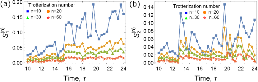
Figure 1: The $\tau$-dependence of the characteristics $S^{(n)}_{1}$ (a) and $S^{(n)}_{2}$ (b). Here $N=6$, $N^{(S)}=N^{(R)}=2$.

Approximation over longer time intervals is worse, as shown by $S_{i}$, $i=3,4$ in Fig. 2.

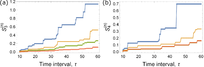
Figure 2: The $\tau$-dependence of the characteristics $S^{(n)}_{3}$ (a) and $S^{(n)}_{4}$ (b). The four lines from bottom to up correspond to the Trotterization number $n$ equal to $60$, $30$, $20$, and $10$, respectively. Here $N=6$, $N^{(S)}=N^{(R)}=2$.

Comparison of the exact evolution of $\lambda_{\max}=\max(\lambda_{\{01\};\{00\}},\lambda_{\{10\};\{00\}})$ with the approximated evolution (with Trotterization number $n=60$) is shown in Fig. 3 for the optimized parameters $\omega^{(n)}$. We see that the approximation is rather good over the whole considered time interval $0\leq{\tau_{\mathrm{reg}}}\leq 60$.

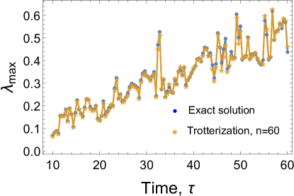
Figure 3: The $\tau$-dependence of the maximal scale factor $\lambda_{\max}=\max(\lambda_{\{01\};\{00\}},\lambda_{\{10\},\{00\}})$. Both the exact and Troterrized ($n=60$) evolutions are shown. Here $N=6$, $N^{(S)}=N^{(R)}=2$.

For completeness, we characterize the values of the parameters $a_{5j}$ used for constructing $S_{1}^{(60)}$ (with the Trotterization number $n=60$) by representing the maximal and minimal (by absolute values) optimizing (minimizing $S_{1}^{(n)}$) parameters $a_{5j}$, $j=1,\dots,4$ ($\min_{j}\,|a_{5j}|$, $\max_{j}\,|a_{5j}|$) as functions of time instant $\tau$ in Fig. 4. By construction, these values are inside of the interval $[0,2]$.

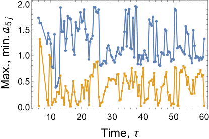
Figure 4: The maximal (upper curve) and minimal (lower curve) values of $a_{5j}$, $j=1,\dots,4$ obtained in constructing $S_{1}^{(60)}$. Here $N=6$, $N^{(S)}=N^{(R)}=2$.

We just add the parameter $\tilde{\varepsilon}$ into the list of the arguments of $S_{i}^{(n)}$ in formulae (40)–(44) with $n=0$. Let us study the dependence of $S_{i}^{(0)}$, $i=1,\dots,5$, on $\varepsilon$. We proceed as follows. First, we set $\varepsilon=1/2$, $\Delta\tau^{(2)}=\Delta\tau^{(1)}$, $\Delta\tau=2\Delta\tau^{(1)}$ and find the parameters $\omega^{(0;m)}=\{a_{51}^{(m)},\dots,a_{54}^{(m)}\}$ as solutions of system (39). It is remarkable that having $\Omega_{j}$ constructed with $\varepsilon=1/2$ ($\Delta\tau^{(2)}=\Delta\tau^{(1)}$), we can deform the obtained result to various $\varepsilon$ with appropriate shrinking of $\tau$ without additional simulating spin dynamics. For a further analysis, it is convenient to introduce the parameter $\tilde{\varepsilon}$ instead of $\varepsilon$ given in (32) and $\tilde{\varepsilon}$-dependent subinterval $\Delta\tau^{(2)}(\tilde{\varepsilon})$ by the formulae

$$\Delta\tau^{(2)}(\tilde{\varepsilon})=\Delta\tau_{1}\tilde{\varepsilon}\;\;\Rightarrow\;\;\tilde{\varepsilon}=\frac{\Delta\tau^{(2)}(\tilde{\varepsilon})}{\Delta\tau_{1}}.$$ (47)

Then, we have

$$\Omega_{j}\Delta\tau^{(1)}=\frac{\Omega_{j}}{\tilde{\varepsilon}}\Delta\tau^{(2)}(\tilde{\varepsilon}).$$

Therefore, we may use the replacement $\displaystyle a_{ij}\to\frac{a_{ij}}{\tilde{\varepsilon}}$ in the Hamiltonian (27), so that condition (28) is satisfied and this condition provides the structure (31) for the Hamiltonian. Because of (47), the interval $\Delta\tau$ becomes also $\tilde{\varepsilon}$-dependent,

$$\Delta\tau(\tilde{\varepsilon})=\Delta\tau^{(1)}+\Delta\tau^{(2)}(\tilde{\varepsilon}).$$

It can be simply verified that $\tilde{\varepsilon}=\varepsilon/(1-\varepsilon)\stackrel{{\scriptstyle\varepsilon\ll 1}}{{\approx}}\varepsilon.$ In this way, we can vary $\tilde{\varepsilon}$ by scaling $\Omega_{j}$ and thus scale $a_{ij}$. In studying the functions $S_{i}^{(0)}$, $i=1,\dots,5$, below we use $\tilde{\varepsilon}$ instead of $\varepsilon$.

The graphs of $S^{(0)}_{i}$, $i=1,\dots,4$, are quite similar to the graphs of $S^{(n)}_{i}$, $i=1,\dots,4$, $n>0$. For instance, the graphs of $S^{(0)}_{i}$, $i=3,4$ as functions of $\tau$ for different $\tilde{\varepsilon}=0.01,\;0.001,\;0.0001$ are shown in Fig. 5.

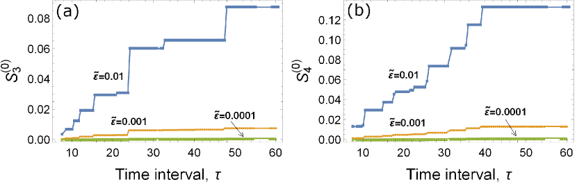
Figure 5: The $\tau$-dependence of the characteristics $S^{(0)}_{3}$ (a) and $S^{(0)}_{4}$ (b) for different $\tilde{\varepsilon}=0.01,\;0.001,\;0.0001$. Here $N=6$ and $N^{(S)}=N^{(R)}=2$.

Notice that since the parameters $a_{5j}$ are represented in the form (46), they are bounded by the condition $|a_{5j}|\in[0,2]$. Of course, the scaled parameters $\displaystyle\frac{a_{5j}}{\tilde{\varepsilon}}$ do not obey this constraint.

Entanglement transfer in state restoring

.

The 2-qubit (0,1)-excitation density matrix is a $4\times 4$ matrix in the form

$$\rho=\left(\begin{array}[]{cccc}\rho_{00}&\rho_{01}&\rho_{02}&0\cr\rho_{10}&\rho_{11}&\rho_{12}&0\cr\rho_{20}&\rho_{21}&\rho_{22}&0\cr 0&0&0&0\end{array}\right).$$ (52)

It was shown in TZarxiv that the bi-particle entanglement measured by the Wootters criterion HW ; Wootters in terms of concurrence can be simply expressed in terms of single element of the 2-qubit density matrix in the case of (0,1)-excitation (see also AQJ ; FYu ), $C=2|\rho_{12}|.$ In the case of state restoring, when $\rho^{(R)}_{12}=\lambda_{12}\rho^{(S)}_{12}$, the ratio $C^{(R)}/C^{(S)}=2|\lambda_{12}|$ does not depend on the sender’s initial state TZarxiv . However, since we deal with approximation models, Model 1 and Model 2, the above statement holds only for them

$$C_{\mathrm{norm}}^{(n)}(\tau)=\frac{C(\rho^{(R;n)}(\tau))}{C(\rho^{(S)}(0))}=2|\lambda_{12}|,\quad C_{\mathrm{norm}}(\tau)=\frac{C(\rho^{(R)}(\tau))}{C(\rho^{(S)}(0))}=f(\rho^{(S)}(0)).$$

Here $\rho^{(R;n)}$ means the density matrix of the 2-qubit receiver state calculated for Model 1 ($n>0$) or Model 2 ($n=0$). The $\tau$-evolution of $C^{(n)}_{\mathrm{norm}}$ is shown in Fig. 6a (Model 1, $n=60$) and in Fig. 6c (Model 2, $\tilde{\varepsilon}=0.0001$) for the EPR initial sender’s state

$$\rho^{(S)}(0)=\frac{1}{2}(|01\rangle+|10\rangle)(\langle 01|+\langle 10|),\quad C(\rho^{(S)}(0))=1.$$

We also introduce the relative discrepancy between the concurrences calculated for Model 1 (Model 2) and for exact solution,

$$\Delta^{(n)}(\tau)=\frac{\left|C(\rho^{(R;n)}(\tau))-C(\rho^{(R)}(\tau))\right|}{C(\rho^{(S)}(0))},$$

whose $\tau$-dependence is shown in Fig. 6b (Model 1, $n=60$) and Fig. 6d (Model 2, $\tilde{\varepsilon}=0.0001$) for the same EPR state.

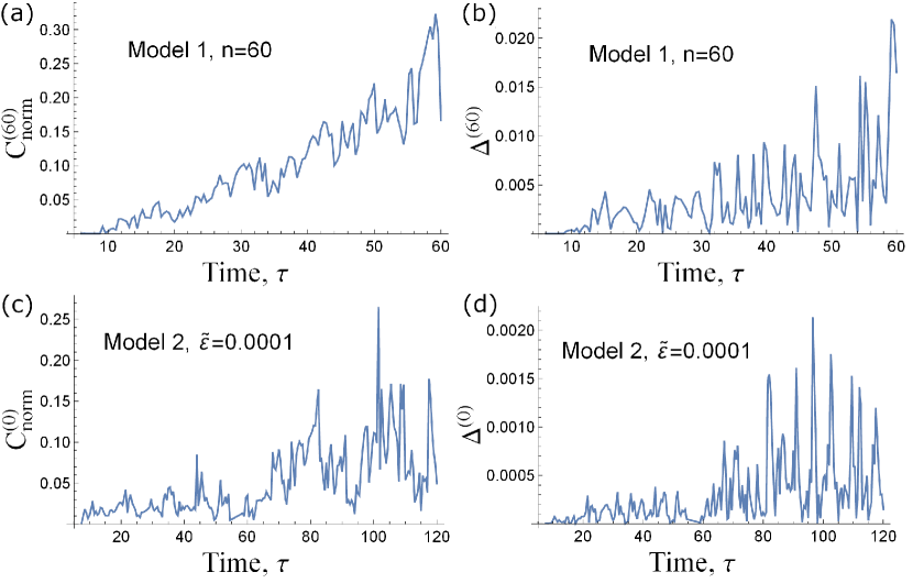
Figure 6: (a) Model 1 with $n=60$, ratio $C^{(60)}_{\mathrm{norm}}$ (b) Model 1 with $n=60$, the relative discrepancy $\Delta^{(60)}$ (c) Model 2 with $\tilde{\varepsilon}=0.0001$, the ratio $C^{(0)}_{\mathrm{norm}}$ (d) Model 2 with $\tilde{\varepsilon}=0.0001$, the relative discrepancy $\Delta^{(0)}$.

Figures 6a and 6c demonstrate that evolution of concurrence in Model 2 is slower than in Model 1 and exhibits high-amplitude oscillations.

II.2.2 Two- and three-qubit state restoring in long chains ($N\leq 20$).

To demonstrate the applicability of the state-restoring protocol to long communication lines, we consider the $N$-dependence of the function $S^{(0)}_{5}$ in the state-restoring of two- and three-qubit states transferred using communication lines with $N\leq 20$. In this section we use only Model 2 and take $\tilde{\varepsilon}=0.0001$, i.e., $\Delta\tau\approx\Delta\tau^{(1)}$.

Two-qubit sender, $N^{(S)}=N^{(R)}=2$.

We plot $\lambda^{(0)}$, given in (45), with fixed $K_{\omega}=5$, as a function of $N$ in Fig. 7. For optimization $S_{5}^{(0)}(T,N)$, we take $T=200N$ and 1000 different solutions $\omega^{(0;m)}$ of the system (39) at $n=0$.

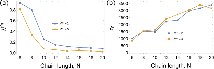
Figure 7: $N^{(S)}=N^{(R)}=2$ and 3; the scale factor $\lambda^{(0)}(N)=S_{5}^{(0)}(\tau_{0},N)$, $0\leq\tau_{0}(N)\leq 200N$, (a) and the corresponding time instant $\tau_{0}(N)$ (b) as functions of the chain length $N$; optimization is over 1000 solutions of Eq. (39) ($n=0$) for $N^{(S)}=2$ and over 2000 solutions for $N^{(S)}=3$.

These graphs demonstrate generic decrease of $\lambda^{(0)}(N)$ and increase of $\tau_{0}(N)$ with $N$. The fact that points of these graphs do not belong to smooth lines is explained, basically, by difficulties in the global optimization of $S^{(0)}_{5}$ according to its definition (44).

Three-qubit sender, $N^{(S)}=N^{(R)}=3$.

We take three nonzero Larmor frequencies, $\omega_{7}$, $\omega_{6}$ and $\omega_{5}$. Eq. (15) yields $\omega_{7}=-\omega_{6}-\omega_{5}$, thus we have two free Larmor frequency $\omega_{5}$ and $\omega_{6}$ which can be used as a control tool. The system (39) consists of 6 complex equations. We have 3 independent scale parameters $\lambda_{i,0}$, $i=1,\;2,\;3$. To satisfy system (39), we take $K_{\omega}=7$, so that there are 14 free parameters $a_{5j}$, $a_{6j}$, $j=1,\dots,7$, generated by $\omega_{5}$ and $\omega_{6}$. Eqs. (39) are considered as a system of equations for these 14 parameters. For optimization in formulas for $S_{5}^{(0)}(T,N)$, we take $T=200N$ and 2000 different solutions of system (39) ($n=0$) $a^{(m)}_{5j}$, $a^{(m)}_{6j}$ or $\tilde{a}^{(m)}_{5j}$, $\tilde{a}^{(m)}_{6j}$ (according to representation (46)), $j=1,\dots,7$, $m=1,\dots,2000$. Finally, we plot $\lambda^{(0)}$ (45) and appropriate $\tau_{0}$ as functions of $N$ in Fig. 7. We see that the line $\lambda^{(0)}$ for $N^{(S)}=3$ is below the line for $N^{(S)}=2$ in Fig. 7a, unlike the lines for $\tau_{0}$ in Fig. 7b.

III Perfect transfer of 0-order coherence matrix along zigzag- and rectangular (multichannel) communication lines

In the recent paper BFLPZ_2022 the perfect transfer of zero-order coherence matrix (PTZ) including up to 1-excitation block governed by the XX-Hamiltonian was studied. That was a simplest nontrivial case, but that PTZ doesn’t allow to include higher-order ($\pm 1$-order) coherence matrices in the process. To make it possible we involve blocks of higher excitation numbers into the density matrix of the initial state. Namely, we consider the initial state of tripartite system including sender ($S$), transmission line ($TL$) and receiver ($R$) in form (2), (3) and assume that the dynamics is governed by XXZ-Hamiltonian (4), (5) with $\Omega=0$. In the case when initial sender state $\rho^{(S)}$ includes only 0-order coherence matrix so that it is a block-diagonal initial sender state, $\rho^{(S)}=\bigoplus_{i=0}^{K}s^{(i)},$ where $s^{(i)}$ is the $i$-excitation block. Thus, the density matrix of the whole $N$-qubit system has the similar block-diagonal form: $\rho=\bigoplus_{i=0}^{K}\sigma^{(i)},$ where $\sigma^{(i)}$ for $N$-qubit system is a $D^{(N)}_{i}\times D^{(N)}_{i}$ matrix, $D^{(N)}_{i}=\left({N}\atop{i}\right)$. Here $K$ is the maximal number of excitations which is restricted by the requirement $K\leq N^{(S)}$. Similarly, for the receiver density matrix ($N^{(R)}=N^{(S)}$) we have $\rho^{(R)}={\mbox{Tr}}_{S,TL}\rho(t)=\bigoplus_{i=0}^{K}r^{(i)}(t).$

III.1 PTZ using whole state space of sender

In this case, $K=N^{(S)}$. It was shown in BFLPZ_2022 , that PTZ in the full state space of sender involves the unitary transformation $U^{\mathrm{ex}}$ (where “ex” means “exchange”) that exchanges two single-element blocks of the receiver’s state space, which are 0- and $N^{(S)}$-excitation blocks, and does not conserve the excitation number, i.e.,

$$[U^{\mathrm{ex}},I_{z}]\neq 0.$$

In this case, the process of the PTZ is most simple and includes two steps.

1. Register the state $\rho^{(R)}$ at some optimal time instant $\tau_{\mathrm{reg}}$ and solve the system

   $$r^{(i)}(\tau_{\mathrm{reg}})=s^{(i)},\quad i=1,2,\dots,N^{(S)}-1,$$ (53)

   $$r^{(N^{(S)})}(\tau_{\mathrm{reg}})=s^{(0)}$$

   for the elements of blocks $s^{(i)}$, $i=0,1,\dots,N^{(S)}-1$. Then, due to the normalization, the following equality holds: $r^{(0)}(\tau_{\mathrm{reg}})=s^{(N^{(S)})}.$

2. Exchange the single-element blocks, $r^{(0)}(\tau_{\mathrm{reg}})\leftrightarrow r^{(N^{(S)})}(\tau_{\mathrm{reg}})$, using the transformation $U^{\mathrm{ex}}$, which in this case is given by

   $$U^{ex}=\left(\begin{array}[]{c|c|c}0&0_{1,2^{N^{(S)}}-2}&1\cr\hline\cr 0_{2^{N^{(S)}}-2,1}&\mathbb{I}_{2^{N^{(S)}}-2,2^{N^{(S)}}-2}&0_{2^{N^{(S)}}-2,1}\cr\hline\cr 1&0_{1,2^{N^{(S)}}-2}&0\end{array}\right),$$ (57)

   where $0_{i,j}$ and $\mathbb{I}_{ij}$ are, respectively, $i\times j$ zero and unit matrices.

As the result, we obtain $\rho^{(R)}(\tau_{\mathrm{reg}})=\rho^{(S)}(0).$ The time instant for state registration can be selected by some additional requirement discussed below. It is important that PTZ in this case can be organized without unitary transformation of the extended receiver.

III.2 PTZ using cut state space of sender

Now, let $K<N^{(S)}$, then only the 0-excitation block is a single-element block. Therefore, we have to create second single-element diagonal block BFLPZ_2022 which will be exchanged with the 0-excitation block by the appropriate transformation $U^{(ex)}$. In principle, any diagonal element in any of two blocks $s^{(1)}$ or $s^{(2)}$ can be singled out by putting zeros for all nondiagonal elements of appropriate row and column. For instance, let the diagonal element of $s^{(2)}$ corresponding to the 1st and 2nd excited qubits be such an element

$$s^{(2)}=\left(\begin{array}[]{c|c}s^{(2)}_{11}&0_{1,D^{(N^{(S)})}_{2}{-1}}\cr\hline\cr 0_{D^{(N^{(S)})}_{2}{-1},1}&\tilde{s}^{(2)}\end{array}\right),\quad D^{(N^{(S)})}_{2}=\left({N^{(S)}}\atop{2}\right),$$ (60)

where $0_{ij}$ is the $i\times j$ zero matrix and $\tilde{s}^{(2)}$ is a $(D^{(N^{(S)})}_{2}-1)\times(D^{(N^{(S)})}_{2}-1)$ matrix.

Evolution under the operator $V(\tau)$ in the block-diagonal form mixes all elements in each $i$-excitation block of the density matrix. Therefore, in general, the block $r^{(2)}$ in the density matrix of the receiver $\rho^{(R)}$ has all nonzero elements

$$r^{(2)}=\left(\begin{array}[]{c|c}r^{(2)}_{1,1}&\bar{r}^{(2)}\cr\hline\cr\Big{(}\bar{r}^{(2)}\Big{)}^{\dagger}&\tilde{r}^{(2)}\end{array}\right),$$ (63)

where $\bar{r}^{(2)}$ is a row of $D^{(N^{(S)})}_{2}{-1}$ elements $\bar{r}^{(2)}_{j}\equiv r^{(2)}_{1{,}j{+1}},\;\;j=1,\dots,D^{(N^{(S)})}_{2}{-1}$, $\tilde{r}^{(2)}$ is a $(D^{(N^{(S)})}_{2}-1)\times(D^{(N^{(S)})}_{2}-1)$ matrix, and we use the fact that $N^{(R)}=N^{(S)}$. To single out the element $r^{(2)}_{11}$ as a one-element block on the diagonal we have to introduce the unitary transformation $U(\varphi)$ of the extended receiver $ER$ (the receiver with several neighboring nodes of the transmission line) at time instant $\tau_{\mathrm{reg}}$. Thus, the free parameters $\varphi$ of the unitary transformation $U$ appear in the elements of $\rho^{(R)}$. Then, we can solve the system

$$\bar{r}^{(2)}=0,$$ (64)

$$\tilde{r}^{(2)}=\tilde{s}^{(2)},\quad r^{(1)}=s^{(1)},\quad r^{(2)}_{11}=s^{(0)}.$$ (65)

In addition, due to the trace-normalization

$$s^{(0)}+s^{(2)}_{11}+\sum_{j}s^{(1)}_{jj}+\sum_{j}\tilde{s}^{(2)}_{jj}=r^{(0)}+r^{(2)}_{11}+\sum_{j}r^{(1)}_{jj}+\sum_{j}\tilde{r}^{(2)}_{jj}=1,$$

we have $r^{(0)}=s^{(2)}_{11}.$ To solve system (64) and (65), we notice that subsystem (65) is a linear system in the elements of $s^{(1)}$ and $\tilde{s}^{(2)}$, $s^{(0)}$. Solving this subsystem and substituting expressions for $s^{(1)}$, $\tilde{s}^{(2)}$ and $s^{(0)}$ into system (64), we obtain a system of nonlinear equations for the parameters $\varphi$ of the unitary transformation of the extended receiver (don’t mix with $U^{\mathrm{ex}}$). Finally we exchange $r^{(0)}\leftrightarrow r^{(2)}_{11}$ using $U^{\mathrm{ex}}$. Then, the state of the receiver at the selected time instant $\tau_{\mathrm{reg}}$ is equal to the initial sender’s state: $\rho^{(R)}(\tau_{\mathrm{reg}})=\rho^{(S)}(0).$

Remark. Solution of system (64) and (65) is not unique due to the presence of extra parameters $\varphi$ in the unitary transformation. A particular solution can be found relatively simply solving Eq. (64) for $\varphi$ (make it identity for all elements of $\rho^{(S)}$) and then solving linear system (65) with constant coefficients for the elements of $\rho^{(S)}$. In fact, $r^{(2)}$ can be represented as TZarxiv

$$r^{(2)}={\mathcal{W}}s^{(2)}{\mathcal{W}}^{\dagger},$$ (66)

where ${\mathcal{W}}$ is some matrix. Therefore, Eq. (64) can be given the following form

$$\bar{r}^{(2)}_{j}\equiv r^{(2)}_{1j}=\sum_{k,n}{\mathcal{W}}_{1k}{\mathcal{W}}^{*}_{jn}s^{(2)}_{kn}.$$

Then, (64) holds if

$${\mathcal{W}}_{1k}=0,\quad k=1,\dots,D^{(N^{(S)})}_{2}.$$ (67)

III.3 Unitary transformation

Let $W$ be the superposition of the evolution $V(\tau)=e^{-iH\tau/D_{12}}$ and unitary transformation of the extended receiver $U(\varphi)$,

$$W(\varphi,\tau)=(\mathbb{I}\otimes U(\varphi))V(\tau),$$

where $\mathbb{I}$ is the unit matrix in the space of the whole system without the extended receiver. The unitary operators $U$ and $W$ have the block-diagonal form

$$U = \bigoplus_{k}U^{(k)}(\varphi^{(k)}),\quad U^{(0)}=1,$$

$$W = \bigoplus_{k}W^{(k)}(\Phi^{(k)}),\quad W^{(0)}=1,\quad\Phi^{(k)}=\{\varphi^{(1)},\dots,\varphi^{(k)}\},$$

where $U^{(i)}$ and $W^{(i)}$ are the blocks corresponding to the subspace of $i$ excitations. The equality $U^{(0)}=1$ is provided by the freedom in the energy of the ground state.

We introduce the multiindexes (35). Then, we can write

$$\rho^{(R)}=\sum_{N_{S},N_{TL}}W_{N_{S}N_{TL}N_{R};I_{S}0_{TL}0_{R}}\rho^{(S)}_{I_{S}J_{S}}W^{\dagger}_{J_{S},0_{TL}0_{R};N_{S}N_{TL}M_{R}}.$$

The number of excitation in the block-diagonal structure of the density matrix varies from 0 to $N^{(S)}$ and thus depends on the dimension of the sender.

III.3.1 $N^{(S)}=3$, (0,1,2,3)-excitation state space.

In the case of 3-qubit sender, we can effectively use up to 3-excitation states, therefore we have only 4 blocks

$$r^{(3)}=W^{(3)}_{0_{S}0_{TL}1_{R};1_{S}0_{TL}0_{R}}(\Phi^{(3)})s^{(3)}_{1_{S}1_{S}}(W^{(3)})^{\dagger}_{1_{S}0_{TL}0_{R};0_{S}0_{TL}1_{R}}(\Phi^{(3)}),$$ (68)

$$r^{(2)}_{N_{R}M_{R}}=\sum_{|N_{S}|+|N_{TL}|=1}W^{(3)}_{N_{S}N_{TL}N_{R};1_{S}0_{TL}0_{R}}(\Phi^{(3)})s^{(3)}_{1_{S}1_{S}}(W^{(3)})^{\dagger}_{1_{S}0_{TL}0_{R};N_{S}N_{TL}M_{R}}(\Phi^{(3)})$$ (69)

$$+\sum_{{I_{S},J_{S}}\atop{|I_{S}|=|J_{S}|=2}}W^{(2)}_{0_{S}0_{TL}N_{R};I_{S}0_{TL}0_{R}}(\Phi^{(2)})s^{(2)}_{I_{S}J_{S}}(W^{(2)})^{\dagger}_{J_{S}0_{TL}0_{R};0_{S}0_{TL}M_{R}}(\Phi^{(2)}),$$

$$\hskip 85.35826pt|N_{R}|=|M_{R}|=2,$$

$$r^{(1)}_{N_{R}M_{R}}=\sum_{|N_{S}|+|N_{TL}|=2}W^{(3)}_{N_{S}N_{TL}N_{R};1_{S}0_{TL}0_{R}}(\Phi^{(3)})s^{(3)}_{1_{S}1_{S}}(W^{(3)})^{\dagger}_{1_{S}0_{TL}0_{R};N_{S}N_{TL}M_{R}}(\Phi^{(3)})$$ (70)

$$+\sum_{|N_{S}|+|N_{TL}|=1}\sum_{|I_{S}|=|J_{S}|=2}W^{(2)}_{N_{S}N_{TL}N_{R};I_{S}0_{TL}0_{R}}(\Phi^{(2)})s^{(2)}_{I_{S}J_{S}}(W^{(2)})^{\dagger}_{J_{S}0_{TL}0_{R};N_{S}N_{TL}M_{R}}(\Phi^{(2)})$$

$$+\sum_{|I_{S}|=|J_{S}|=1}W^{(1)}_{0_{S}0_{TL}N_{R};I_{S}0_{TL}0_{R}}(\Phi^{(1)})s^{(1)}_{I_{S}J_{S}}(W^{(1)})^{\dagger}_{J_{S}0_{TL}0_{R};0_{S}0_{TL}M_{R}}(\Phi^{(1)}),$$

$$\hskip 85.35826pt|N_{R}|=|M_{R}|=1,$$

$$r^{(0)}=1-{\mbox{Tr}}(r^{(1)})-{\mbox{Tr}}(r^{(2)})-r^{(3)}.$$

In the case of three-qubit sender, the system (53) reduces to the following one

$$r^{(i)}(\tau_{\mathrm{reg}})=s^{(i)},\quad i=1,2,\quad r^{(3)}(\tau_{\mathrm{reg}})=s^{(0)}.$$ (71)

Solving this system for the elements of $s^{(i)}$ we obtain the perfectly transferable 0-order coherence matrix.

III.3.2 $N^{(S)}\geq 3$, (0,1,2)-excitation state space.

Now we consider initial state with no more then 2 excitations. In this case $r^{(3)}=s^{(3)}=0$, eq.(68) disappears, while equations (69) and (70) get the following form

$$r^{(2)}_{N_{R}M_{R}}=\sum_{|I_{S}|=|J_{S}|=2}W^{(2)}_{0_{S}0_{TL}N_{R};I_{S}0_{TL}0_{R}}(\Phi^{(2)})s^{(2)}_{I_{S}J_{S}}(W^{(2)})^{\dagger}_{J_{S}0_{TL}0_{R};0_{S}0_{TL}M_{R}}(\Phi^{(2)}),$$ (72)

$$\hskip 85.35826pt|N_{R}|=|M_{R}|=2,$$

$$r^{(1)}_{N_{R}M_{R}}=\sum_{|N_{S}|+|N_{TL}|=1}\sum_{|I_{S}|+|J_{S}|=2}W^{(2)}_{N_{S}N_{TL}N_{R};I_{S}0_{TL}0_{R}}(\Phi^{(2)})s^{(2)}_{I_{S}J_{S}}(W^{(2)})^{\dagger}_{J_{S}0_{TL}0_{R};N_{S}N_{TL}M_{R}}(\Phi^{(2)})$$

$$+\sum_{|I_{S}|+|J_{S}|=1}W^{(1)}_{0_{S}0_{TL}N_{R};I_{S}0_{TL}0_{R}}s^{(1)}_{I_{S}J_{S}}(\Phi^{(1)})(W^{(1)})^{\dagger}_{J_{S}0_{TL}0_{R};0_{S}0_{TL}M_{R}}(\Phi^{(1)}),$$

$$\hskip 85.35826pt|N_{R}|=|M_{R}|=1.$$

Note that Eq. (72) is equivalent to Eq. (66) up to the change of notation $W^{(2)}\to{\mathcal{W}}$. To arrange the structure (60) we require

$$W^{(2)}_{0_{S}0_{TL}\{110\dots 0\};I_{S}0_{TL}0_{R}}(\Phi^{(2)})=0,$$

which is equivalent to (67).

III.4 Zigzag spin chain, $N^{(S)}=3$

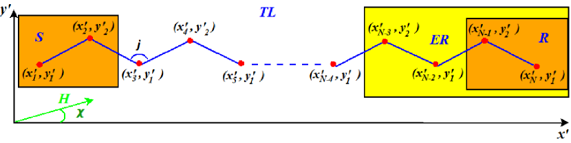
Figure 8: Zigzag spin 1/2 chain.

We use the $XXZ$ Hamiltonian (5) with $D_{ij}$ taking into account the orientation of the external magnetic field,

$$H_{XXZ}=\sum_{j>i}\frac{\gamma^{2}}{2r^{3}_{ij}}(3\cos^{2}\varphi_{ij}-1)(X_{i}X_{j}+Y_{i}Y_{j}-2Z_{i}Z_{j}).$$ (73)

Let $j$th spin have coordinates $(x_{j},y_{j})$, the magnetic field ${\mathrm{H}}$ is directed at the angle $\chi$ to the chain axis. In the system $(x^{\prime},y^{\prime})$, the unit vector $\mathrm{n}$ has coordinates ${\mathrm{n}}=(\cos\chi,\sin\chi)$. Then,

$${\mathrm{r}}_{ij}=(x^{\prime}_{j}-x^{\prime}_{i},y^{\prime}_{j}-y^{\prime}_{i}),$$ (74)

$$r_{ij}=\sqrt{(x^{\prime}_{j}-x^{\prime}_{i})^{2}+(y^{\prime}_{j}-y^{\prime}_{i})^{2}},\quad\cos\varphi_{ij}=\frac{(x^{\prime}_{j}-x^{\prime}_{i})\cos\chi+(y^{\prime}_{j}-y^{\prime}_{i})\sin\chi}{r_{ij}}.$$

We consider

$$x^{\prime}_{j}=\Delta(j-1),\quad y^{\prime}_{j}=\left\{\begin{array}[]{ll}0,&j=1,3,5,\dots,\cr y_{0},&j=2,4,6,\dots,\end{array}\right.$$ (77)

i.e., the $y^{\prime}$-coordinate takes two values, either $0$ or $y_{0}$. We use $\chi$ and $y_{0}$ as two free parameters characterizing the chain geometry, Fig. 8. The communication line includes the sender ($S$), transmission line ($TL$) and receiver ($R$), see Fig. 8. In addition, the extended receiver ($ER$) serves to correct the receiver’s state via the unitary transformation applied to it. In this section we use the dimensionless time $\tau={t\gamma^{2}}/{\Delta^{3}}.$

We consider the 3-qubit sender and receiver in the 9-qubit communication system $(N=9)$ under the XXZ Hamiltonian (73). We are aimed at optimizing the perfectly transferred 0-order coherence matrix including 0-, 1- and 2-excitation blocks (without 3-excitation block). We say that the matrix is optimized if its minimal diagonal element $\delta_{d}$ in the 1- and 2-excitation blocks (except the element which is subjected to the operation $U^{(ex)}$ in n. 2 below) takes the maximum possible value. We solve this problem in two steps.

1. Let us consider the system with up to 3 excitations. In this case, according to BFLPZ_2022 , elements with 0 and 3 excitations can be exchanged on the last step of restoring. For fixed parameters of the chain $\chi$ and $y_{0}$, we find such optimal time instant $\tau_{0}$ that maximizes $\delta_{d}$. Thus, we obtain the distributions of $\delta_{d}$ and $\tau_{0}$ on the plane $(y_{0},\chi)$ shown in Fig. 9.

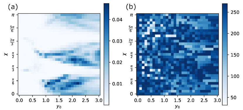
Figure 9: (a) The parameter $\delta_{d}$ optimized over time $\tau$ and (b) corresponding optimal time instant $\tau_{0}$ as functions of $y_{0}$ and $\chi$. The region $\chi=\pi/2$, $1\lesssim y_{0}\lesssim 1.6$ can be considered to be optimal. In this case $\delta_{d}\sim 0.35$.

The parameter $\delta_{d}$ has large values in the dark region on the plane $(y_{0},\chi)$ (see Fig. 9a), where $\chi=\pi/2$, $1\lesssim y_{0}\lesssim 1.6$. The same region of large values of $\delta_{d}$ remains for different lengths of communication system and for cases of lower excitation space. In this case, $\delta_{d}\sim 0.35$. We turn to this region.

2. Now we pass to the problem of optimal transfer of the 0-order coherence matrix with up to 2-excitation blocks. In this case, to provide structure (60) for the 2-excitation block, we have to solve the system of equations (64) and (65) for the parameters of the unitary transformation of the extended receiver (4-qubit subsystem in our case). After that we exchange positions of two singled out elements of the receiver and thus construct the perfectly transferred 0-order coherence matrix including up to 2-excitation block with $N^{(S)}=3$.

Time-dependence of the parameter $\delta_{d}$, and the accuracy of transformation of the above pointed elements to zero are shown in Fig. 10 for several values of the parameter $y_{0}$. We see that all selected values of $y_{0}$ yield much the same result, the parameter $\delta_{d}$ takes the maximal value $\approx 0.9$ at $\tau_{\mathrm{reg}}\approx 183$ for $y_{0}=1.3$. This is the recommended time instant for the receiver’s state registration.

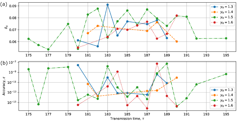
Figure 10: Time-dependence of (a) the parameter $\delta_{d}$ and (b) the accuracy of calculation of the transferred-to-zero elements for several values of the parameter $y_{0}$.

III.5 Rectangular (multichannel) spin chain

Now we consider the $K$-channel lattice shown in Fig. 11. The Hamiltonian is the same, Eq. (73). The coordinates $x^{\prime}_{n}$ and $y^{\prime}_{n}$ of the $n$th spin are following

$$x^{\prime}_{n}=[(n-1)/K]\Delta_{x},\quad y^{\prime}_{n}=(n-1-K[(n-1)/K])\Delta_{y},\quad\frac{N}{K}\in\mathbb{Z},$$

where $[\cdot]$ means the integer part of a number. We introduce the dimensionless time $\tau={t\gamma^{2}}/{\Delta^{3}_{x}}$ and assume that $\Delta_{y}$ and $\chi$ are free parameters. Formulas (74) and (III.4) are applicable in this case as well.

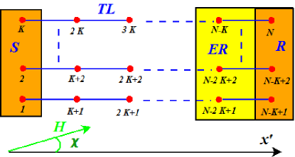
Figure 11: Spin 1/2 lattice, $K$ is the number of channels.

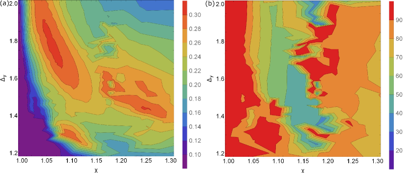
Figure 12: (a) Parameter $\delta$ optimized over $\tau$ as a function of $\Delta_{y}$ and $\chi$; (b) the optimal time instant $\tau_{0}$ for the state registration as a function of $\Delta_{y}$ and $\chi$.

We consider the propagation of the 3-qubit state along the three-channel communication line ($K=3$ in Fig.11) with 10 spins in each channel (the 30-qubit system). Solving the system (71), we find the $\tau$-dependence for $\rho^{(S)}(\tau)$. After that we find $\tau_{0}$ that maximizes the norm $\delta(\tau,\Delta_{y},\chi)$, similar to BFLPZ_2022 :

$$\delta(\tau)=||\rho^{(R)}_{\infty}-\rho^{(R)}(\tau)||,$$

i.e., $\delta(\tau_{0})=\max_{\tau}\delta(\tau).$ Here $\rho^{(R)}_{\infty}={\mbox{diag}}(1,\underbrace{0,\dots,0}_{2^{K}-1})$ is an asymptotic matrix BFLPZ_2022 . The contour graphs of $\delta(\tau_{0},\Delta_{y},\chi)$ and of corresponding time instances $\tau_{0}$ over the plane $(\Delta_{y},\chi)$ are shown in Figs. 12$a$ and 12$b$. The red region on the plane $(\Delta_{y},\chi)$ in Fig. 12$a$ ($\{1.04\lesssim\chi\lesssim 1.08;1.65\lesssim\Delta_{y}\lesssim 1.90\}$) corresponds to $\delta\gtrsim 0.3$ at $\tau_{0}\sim 60\div 80$. The time instant for state registration $\tau_{\mathrm{reg}}$ should be taken from that interval.

IV Analytical approach

The analytical approach allows us to effectively study the long-time dynamics which is especially important for the XXZ model which requires much longer times for state transfer along a spin chain PRA2010 . The analytical formulas were developed in PRA2010 for the homogeneous chain with remote end-nodes (in particular, the homogeneous chain which we adopt here, see also FR ; KF ) and nearest-neighbor approximation, i.e.,

$$H_{XXZ}=\sum_{j=1}^{N-1}D(X_{j}X_{j+1}+Y_{j}Y_{j+1}-2Z_{j}Z_{j+1}).$$

Due to the block-diagonal structure (14) of the Hamiltonian, we can consider the evolution in 0- and 1-excitation subspaces separately. The 1-excitation subspace is an $N\times N$ space, and 0-excitation subspace is a one-dimensional space.

We use the diagonalization of the one-excitation block $H^{(1)}$ proposed in PRA2010 . Elements of the eigenvector $u_{j}$ are given by

$$u_{kj}=\left\{\begin{array}[]{ll}\displaystyle A_{j}\cos\frac{(N+1-2k)p_{j}}{2},&k=1,...N,\;\;j=1,\dots N_{1},\cr\displaystyle A_{j}\sin\frac{(N+1-2k)p_{j}}{2},&k=1,...N,\;\;j=N_{1}+1,\dots N.\end{array}\right.$$

The appropriate eigenvalues are defined as follows: $\lambda_{j}=D\cos p_{j}.$ Here the parameters $p_{j}$ satisfy the following system

$$2\cos{\frac{N-1}{2}p_{j}}+\cos{\frac{N+1}{2}p_{j}}=0,\quad j=1,\dots,N_{1},\quad N_{1}=N-\left[\frac{N}{2}\right],$$

$$2\sin{\frac{N-1}{2}p_{j}}+\sin{\frac{N+1}{2}p_{j}}=0,\quad j=N_{1}+1,\dots,N,$$

and the normalization constants $A_{j}$ are given by

$$A_{j}=\left\{\begin{array}[]{ll}\displaystyle\left(\frac{N-2}{2}+({1+\cos(N-1)p_{j}})+\frac{\sin(N-2)p_{j}}{2\sin p_{j}}\right)^{-1/2},&j=1,\dots,N_{1},\cr\displaystyle\left(\frac{N-2}{2}+({1-\cos(N-1)p_{j}})-\frac{\sin(N-2)p_{j}}{2\sin p_{j}}\right)^{-1/2},&j=N_{1}+1,\dots,N.\end{array}\right.$$ (80)

We consider the 2-qubit sender and receiver ($N^{(S)}=N^{(R)}=2$) with the initial density matrix (2) and (3), where

$$\rho^{(S)}(0)={\mbox{diag}}(a_{00},\rho^{(S;1)}),\quad\rho^{(S;1)}=\begin{pmatrix}a_{11}&a_{12}\\ a^{*}_{12}&a_{22}\\ \end{pmatrix}.$$ (81)

Here $a_{00}$ (scalar) and $\rho^{(S;1)}$ are blocks of the sender’s initial state including 0- and 1-excitation subspaces, $a_{00}$ does not evolve. Evolution of the one-excitation block is described by the operator $U^{(1)}=\exp(-i{H^{(1)}}\tau/D)$, where $\tau$ is the dimensionless time (16), $D_{12}=D$. We have

$$\rho(t)=\rho_{0,0}|0\rangle\langle 0|+\sum_{\stackrel{{\scriptstyle i,j=1}}{{i^{\prime},j^{\prime}=1}}}^{N}\sum_{m,m^{\prime}=1}^{2}u_{ij}u^{*}_{i^{\prime}j^{\prime}}e^{-i(\lambda_{j}-\lambda_{j^{\prime}})\tau/D}\rho^{(S)}_{m,m^{\prime}}(0)u^{*}_{mj}u_{m^{\prime}j^{\prime}}|i\rangle\langle i^{\prime}|.$$

The receiver’s density matrix (33) reads

$$\rho^{(R)}(\tau_{\mathrm{reg}})=\begin{pmatrix}\rho_{0,0}^{(R)}(\tau_{\mathrm{reg}})&0&0\\ 0&\rho^{(R)}_{1,1}(\tau_{\mathrm{reg}})&\rho^{(R)}_{1,2}(\tau_{\mathrm{reg}})\\ 0&(\rho^{(R)}_{1,2})^{*}(\tau_{\mathrm{reg}})&\rho^{(R)}_{2,2}(\tau_{\mathrm{reg}})\end{pmatrix}$$

$$=\begin{pmatrix}\rho_{0,0}+\sum_{j=1}^{N-2}{\rho_{j,j}(\tau_{\mathrm{reg}})}&0&0\\ 0&\rho_{N-1,N-1}(\tau_{\mathrm{reg}})&\rho_{N-1,N}(\tau_{\mathrm{reg}})\\ 0&\rho_{N,N-1}(\tau_{\mathrm{reg}})&\rho_{N,N}(\tau_{\mathrm{reg}})\end{pmatrix}.$$

Next, we fix the elements $a_{ij}$ in (81) by imposing the following relation among the elements of $\rho^{(R)}(\tau_{\mathrm{reg}})$, fixed at some time instant for state registration $\tau_{\mathrm{reg}}$ (specified below), and the elements $a_{ij}$:

$$a_{12}=\rho^{(R)}_{12}(\tau_{\mathrm{reg}}),\quad a_{22}=\rho_{2,2}^{(R)}(\tau_{\mathrm{reg}}),\quad a_{00}=\rho_{11}^{(R)}(\tau_{\mathrm{reg}}).$$

As a characteristic of the remote state restoring, we introduce the function

$$S(N)=\max_{0<\tau\lesssim 10^{3N/10}}|a_{12}(\tau)|.$$

We denote $\tau_{0}(N)$ the time instant $\tau$ corresponding to $S(N)$, i.e., $S=|a_{12}(\tau_{0}(N))|$. $N$-dependence of $S$ and $\tau_{0}$ is shown in Fig. 13. Thus, the state-transfer time $\tau_{\mathrm{reg}}=\tau_{0}$ increases exponentially with $N$.

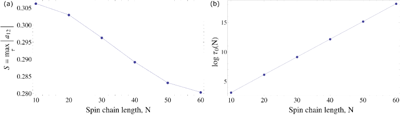
Figure 13: $N$-dependence of the parameter (a) $S$ and (b) $\tau_{0}(S)$.

V Conclusions

In this work we present several aspects of evolution of spin chains with XXZ-Hamiltonian. First, we consider the state-restoring protocol with the time-dependent Larmor frequencies as a controlling tool. To provide optimization of the remote state transfer, we implement two approximating models. Model 1 uses Trotterization and Model 2 uses short magnetic pulses of certain amplitude, similar to that considered in FPZ_Archive2023 for the XX-Hamiltonian. We use the quantities $S_{i}^{(n)}$ for $i=1,\dots,4$ to describe the accuracy of the approximation and the quantity $S_{5}^{(n)}$ to describe the quality of the state restoring, i.e., the absolute values of $\lambda$-factors. This parameter as a function of chain length $N$ decreases with an increase of $N$ and, for fixed $N$, reaches its maximal value at sufficiently long times, much longer than for the XX-model. The confirmation of the long-time evolution is presented in the theoretical consideration of the 0-order coherence transfer, where exponential increase of the state-transfer time with the chain length $N$ is found. We also study the two-qubit concurrence evolution in the state-restoring process and discrepancy in its calculation using an approximate model and exact spin-chain evolution. The perfect transfer of the 0-order coherence matrix including the 0-, 1-, 2- and 3-excitation blocks is also considered for non-linear communication lines such as the zigzag chain and rectangular configuration which is a multichannel line. The geometric parameters optimizing such transfer are found. To provide the required structure of the transferred state, where certain elements must be zero after transfer of 0-order coherence matrix, we use a unitary transformation of the extended receiver (we consider a 4-qubit extended receiver for a 3-qubit receiver). These aspects of the spin chain evolution under XXZ-Hamiltonian outline features typical for this Hamiltonian and can be useful for further development of quantum information transfer in solids.

Funding

This work was funded by Russian Federation represented by the Ministry of Science and Higher Education of Russian Federation (grant number 075-15-2020-788).

References

- (1) S. Bose, “Quantum communication through an unmodulated spin chain, ”Phys. Rev. Lett. 91, 207901 (2003).
- (2) M. Christandl, N. Datta, A. Ekert, and A. J. Landahl , “Perfect state transfer in quantum spin networks, ”Phys. Rev. Lett. 92, 187902 (2004).
- (3) P. Karbach and J. Stolze, “Spin chains as perfect quantum state mirrors, ”Phys. Rev. A. 72, 030301(R) (2005).
- (4) G. Gualdi, V. Kostak, I. Marzoli, and P. Tombesi, “Perfect state transfer in long-range interacting spin chains, ”Phys. Rev. A. 78, 022325 (2008).
- (5) A. I. Zenchuk, “Partial structural restoring of two-qubit transferred state, ”Phys. Lett. A 382, 3244 (2018).
- (6) G. A. Bochkin, E. B. Fel’dman, I. D. Lazarev, A. N. Pechen, and A. I. Zenchuk, “Transfer of zero-order coherence matrix along spin-1/2 chain, ”Quant. Inf. Proc. 21, 261 (2022).
- (7) L. Aubourg and D. Viennot, “Information transmission and control in a chaotically kicked spin chain, ”J. Phys. B: At. Mol. Opt. Phys. 49 (11), 115501 (2016).
- (8) H. J. Shan, C. M. Dai, H. Z. Shen, and X. X. Yi, “Controlled state transfer in a Heisenberg spin chain by periodic drives, ”Sci. Rep. 8 (1), 13565 (2018).
- (9) P. V. Pyshkin, E. Y. Sherman, J. Q. You, and L.-A. Wu, “High-fidelity non-adiabatic cutting and stitching of a spin chain via local control, ”New J. Phys. 20 (10), 105006 (2018).
- (10) A. Ferrón, P. Serra, and O. Osenda, “Understanding the propagation of excitations in quantum spin chains with different kind of interactions, ”Phys. Scr. 97 (11), 115103 (2022).
- (11) A. Pechen and H. Rabitz, “Teaching the environment to control quantum systems, ”Phys.Rev.A 73, 062102 (2006).
- (12) A. Pechen, N. Il’in, F. Shuang, and H. Rabitz, “Quantum control by von Neumann measurements, ”Phys. Rev. A 74, 052102 (2006).
- (13) A. Yu. Kitaev, A. H. Shen, and M. N. Vyalyi, Classical and Quantum Computation. Graduate Studies in Mathematics 47 (American Mathematical Society, Providence, Rhode Island, 2002).
- (14) M. A. Nielsen and I. L. Chuang, Quantum Computation and Quantum Information (Cambridge: Cambridge Univ. Press., p. 676, 2010).
- (15) E. B. Fel’dman, A. N. Pechen, and A. I. Zenchuk, “Optimal remote restoring of quantum states in communication lines via local magnetic field, ”Phys. Scr. 99, 025112 (2024)
- (16) V. Petruhanov and A. Pechen, “GRAPE optimization for open quantum systems with time-dependent decoherence rates driven by coherent and incoherent controls, ”J. Phys. A: Math. Theor. 56, 305303 (2023).
- (17) O. Morzhin and A. Pechen, “Optimal state manipulation for a two-qubit system driven by coherent and incoherent controls, ”Quant. Inf. Proc. 22, 241 (2023).
- (18) E. B. Fel’dman, E. I. Kuznetsova, and A. I. Zenchuk, “High-probability state transfer in spin-1/2 chains: Analytical and numerical approaches, ”Phys. Rev. A 82, 022332 (2010).
- (19) A. Abragam, The principles of nuclear magnetism (Oxford, Clarendon press, 1961).
- (20) H. F. Trotter, “On the product of semi-groups of operators, ”Proc. Amer. Math. Soc. 10 (4), 545–551 (1959).
- (21) M. Suzuki, “Generalized Trotter’s formula and systematic approximants of exponential operators and inner derivations with applications to many-body problems, ”Commun. Math. Phys. 51 (2), 183–190 (1976).
- (22) N. A. Tashkeev and A. I. Zenchuk, “Remote restoring of (0,1)-excitation states and concurrence scaling, ”arXiv:2310.04526 [quant-ph] (2023).
- (23) K. Kraus, States, effects, and operations: fundamental notions of quantum theory (Springer, Berlin Heidelberg, 1983).
- (24) S. Hill and W. K. Wootters, “Entanglement of a pair of quantum bits, ”Phys. Rev. Lett. 78, 5022 (1997).
- (25) W. K. Wootters, “Entanglement of formation of an arbitrary state of two qubits, ”Phys. Rev. Lett. 80 2245 (1998).
- (26) A. Al-Qasimi and D. F. V. James, “Sudden death of entanglement at finite temperature, ”Phys. Rev. A 77, 012117 (2008).
- (27) A.V. Fedorova and M. A. Yurischev, “Quantum entanglement in the anisotropic Heisenberg model with multicomponent DM and KSEA interactions, ”Quant. Inf. Proc. 20, 169 (2021).
- (28) E. B. Fel’dman and M. G. Rudavets, “Exact results on spin dynamics and multiple quantum NMR dynamics in alternating spin-1/2 chains with XY Hamiltonian at high temperatures, ”JETP Letters 81 (2), 47–52 (2005).
- (29) E. I. Kuznetsova and E. B. Fel’dman, “Exact solutions in the dynamics of alternating open chains of spins s = 1/2 with the XY Hamiltonian and their application to problems of multiple-quantum dynamics and quantum information theory, ”JETP 102 (6), 882 (2006).