Data-Driven Optimal Feedback Laws via
Kernel Mean Embeddings

Abstract

This paper proposes a fully data-driven approach for optimal control of nonlinear control-affine systems represented by a stochastic diffusion. The focus is on the scenario where both the nonlinear dynamics and stage cost functions are unknown, while only control penalty function and constraints are provided. Leveraging the theory of reproducing kernel Hilbert spaces, we introduce novel kernel mean embeddings (KMEs) to identify the Markov transition operators associated with controlled diffusion processes. The KME learning approach seamlessly integrates with modern convex operator-theoretic Hamilton-Jacobi-Bellman recursions. Thus, unlike traditional dynamic programming methods, our approach exploits the “kernel trick” to break the curse of dimensionality. We demonstrate the effectiveness of our method through numerical examples, highlighting its ability to solve a large class of nonlinear optimal control problems.

I Introduction

Performance and complexity challenges in cyber-physical system, such as power and smart grids [16, 54, 38], robotic manipulators [40, 44], aerospace [43] or autonomous vehicles [42, 28] underscore the paramount importance of optimal control theory. Traditionally, this theory relies on Bellman’s principle of optimality and the associated Hamilton-Jacobi-Bellman (HJB) equation [4, 19]. While these theoretical constructs offer a robust mathematical backbone, their practical deployment for achieving globally optimal control solutions faces formidable obstacles, particularly in high-dimensional state spaces. In such scenarios, local optimal control approaches, such as direct methods combined with sequential quadratic programming or interior points solvers [9, 10] have demonstrated superior performance over dynamic-programming approaches that aim for global optimality. This superiority stems from the notorious ”curse of dimensionality,” which plagues the global resolution of HJB equations, even for problems of moderate scale [61]. However, this paper breaks the inherent curse of dimensionality in HJB formulations by leveraging stochastic control system models that are either directly inferred from experimental data or generated by randomized sampling. This is due to the fact that machine learning methods, e.g. kernel methods, can make both sample and time complexity effectively free of state-dimensionality.

As such, data-driven operator-theoretic approaches to stochastic optimal control represent a paradigm shift, holding the promise of revolutionizing the way we tackle intricate optimal control challenges across a diverse spectrum of cyber-physical systems. Inspired by the flexibility of modern machine learning methods, this paper makes a step towards learning control system representations that could unlock the full potential of system-theoretic models in downstream tasks such as optimal control. This is enabled by recent advances in kernel-based operator-theoretic learning methods [37, 35, 6], that have the ability to learn a control system model directly from a single dataset using nonparametric operator learning techniques [7].

TABLE I: Comparison to state-of-the-art data-driven optimal feedback design approaches for nonlinear control systems.

Attribute	[13]	[60]	[45]	this work
large system class	✗	✓	✓	✓
weak stability requirements	✗	✗	✗	✓(GC)
unknown stage cost	✗	✗	✗	✓
unknown dynamics	✓	✓	✗	✓
value convergence rate	✓	✗	✗	$\text{\char 51}(\texttt{{Thm.}~{}\ref{thm::convergence}})$

Our work builds on these techniques to enable handling stochastic control systems and optimal control design in flexible, infinite-dimensional, Reproducing Kernel Hilbert Spaces (RKHSs), which have a rich history in machine learning and strong theoretic foundations [58]. By embedding probability distributions in RKHSs using the theory of kernel mean embeddings (KMEs) [49], we overcome the curse of dimensionality of dynamic programming by applying the so-called “kernel trick” to stochastic control systems. As a consequence, the complexity of finding the optimal controllers from data is of the same order as for kernel-based system-identification.

I-A Literature Review

Models for stochastic diffusion processes trace their origins to the pioneering works of Fokker [20], Planck [52], and Kolmogorov [31]. These seminal contributions have laid the foundation for the development of modern techniques in analyzing stochastic diffusion processes. A comprehensive overview of the state-of-the-art in this field can be found in [11], which provides an in-depth discussion of modern analysis techniques for studying the associated Fokker-Planck-Kolmogorov (FPK) equations and their underlying Markov processes. Stochastic optimal control problems have since emerged as a natural extension of these models, initially explored by Wonham [63] and further developed by Puterman [55]. Their contributions have significantly shaped the modern stochastic control theory landscape. Fleming and Soner’s book [19], Crandall, Ishii, and Lions’ user guide [14], and Krylov’s textbook on stochastic diffusion processes [39] offer comprehensive treatments of the stochastic extensions of the Hamilton-Jacobi-Bellman (HJB) equation, which are integral to stochastic optimal control. Additionally, [27] provides a more updated review of these methods.

A noteworthy trend in recent years is the systematic exploitation of operator-theoretic system models, particularly those based on Koopman operators [32, 33, 47]. This approach, which has gained momentum in recent years [8, 34], holds promise in solving nonlinear optimal control problems to global optimality through linear embedding methods [27, 61, 62]. Although related operator-theoretic system identification methods are arguably still in their developmental stages, an interesting aspect is the possibility of identifying the transition operators of controlled Markov processes using kernel regression techniques [6, 30, 37]. These methods share a commonality in using the ”kernel trick” to overcome the curse of dimensionality that often arises in data-driven nonlinear system identification [1, 5]. This approach enables the effective handling of complex nonlinear relationships in high-dimensional data, ensuring the robustness and reliability of these methods in various applications. For a comprehensive review of the properties of kernel mean embedding operators, we refer to the work of Muandet et al. [49].

While there is a recent growth in interest for optimal control design using operator-theoretic machinery [25], existing works do not come with value function convergence rates [60, 48, 45] or consider finite-dimensional spaces [13] and strong requirements related to stability properties as well as known stabilizing controllers [51, 45], see Table I.

I-B Contributions

The main contributions of this article are:

1. Fully data-driven: We provide the first nonparametric approach for learning control diffusion processes and forecast state distributions and conditional means for control-affine systems.

2. Breaking the “curse” via KMEs: We exploit the kernel trick to break the curse of dimensionality of HJB by systematically deriving kernel mean embeddings for stochastic optimal control – a first in the literature.

3. Minimal assumptions: Our approach requires no stability or prior knowledge restrictions – unprecedented in existing literature (see Table I).

4. Learning guarantees: Our in-depth analysis of value function convergence rates provides the first-of-its-kind results for estimating optimal control laws for control-affine systems based solely on data (see Theorem 3).

Organization This article is organized as follows. Section II introduces stochastic nonlinear control-affine optimal problems and reviews methods for reformulating them as equivalent Partial Differential Equation (PDE) constrained optimization problem. Section III leverages KMEs and the equivalence between RKHS feature maps and test functions for defining weak solutions of PDEs, leading to a convex, measure-theoretic optimal control problem. Section IV introduces a data-driven approximation of the aforementioned optimal control problem, which can be efficiently solved via a simple Kernel Hamilton Jacobi Bellman recursion (KHJB). Finally, Section V applies the proposed method to benchmark optimal control problems illustrating its computational effectiveness, numerical accuracy, and practical performance.

I-C Notation

Let $\mathbb{X}\subseteq\mathbb{R}^{n}$ be an open domain. We use the symbol $\mathbb{B}\left(\mathbb{X}\right)$ to denote the set of Borel sets of $\mathbb{X}$. Similarly, $M_{+}(\mathbb{X})$ denotes the set of non-negative bounded Borel measures on $\mathbb{X}$ and $M(\mathbb{X})$ the corresponding set of bounded signed Borel measures. Similarly, $D_{+}(\mathbb{X})$ denotes the set of non-negative bounded distributions on $\mathbb{X}$. Let $\mu\in M_{+}(\mathbb{X})$ be a measure with full support, $\mathrm{supp}(\mu)=\mathbb{X}$. The symbols $C^{k}(\mathbb{X})$, $L_{\mu}^{k}(\mathbb{X})$, $H_{\mu}^{k}(\mathbb{X})$ represent—as usual—the set of $k$-times continuously differentiable, $L_{\mu}^{k}$-integrable, and $k$-times weakly differentiable functions with $L_{\mu}^{2}$-integrable derivatives. Moreover, we recall that $L_{\mu}^{2}(\mathbb{X})=H_{\mu}^{0}(\mathbb{X})$ and $H_{\mu}^{k}(\mathbb{X})$ are Hilbert space with standard inner products

$$\langle\phi,\psi\rangle:=\textstyle\sum_{j=0}^{k}\int_{\mathbb{X}}\nabla^{j}\phi\nabla^{j}\psi\,\mathrm{d}\mu.$$

For the special case that $\mathrm{d}\mu=\mathrm{d}{\bm{x}}$ is the standard Lebesgue measure, we skip the index $\mu$. For example, $L^{2}(\mathbb{X})$ denotes the standard $L^{2}$-space. The dual Hilbert space of any given Hilbert space $H$ is denoted by $H^{*}$. Moreover, $W(0,T;L_{\mu}^{2}(\mathbb{X}),H_{\mu}^{1}(\mathbb{X}))$ denotes the set of strongly measurable functions from the time interval $[0,T]$ to $H_{\mu}^{1}(\mathbb{X})$, $\phi\in L^{2}(0,T;H_{\mu}^{1}(\mathbb{X}))$, whose weak time-derivative $\dot{\phi}$ is a strongly measurable function from $[0,T]$ to $H_{\mu}^{1}(\mathbb{X})^{*}$, such that $\dot{\phi}\in L^{2}(0,T;H_{\mu}^{1}(\mathbb{X})^{*})$.

Finally, for the case that $\mathsf{X}=\left[\bm{x}^{(1)},\ldots,\bm{x}^{(N)}\right]\in\mathbb{R}^{n\times N}$ denotes a data matrix, whose columns consist of $N$ data points, and $f:\mathbb{R}^{n}\to\mathbb{R}$ a scalar function, then the notation

$$f(\mathsf{X}):=\ \left[f(\bm{x}^{(1)}),\ldots,f(\bm{x}^{(N)})\right]^{\intercal}\in\mathbb{R}^{N}$$

is used to denote the vector that is obtained by evaluating $f$ at all columns of $\mathsf{X}$. Similarly, for two given data matrices $\mathsf{Y}=\left[\bm{y}^{(1)},\ldots,\bm{y}^{(N_{a})}\right]$ and $\mathsf{Z}=\left[\bm{z}^{(1)},\ldots,\bm{z}^{(N_{b})}\right]$ and a given kernel $k:\mathbb{R}^{n}\times\mathbb{R}^{n}\to\mathbb{R}$, we use the following shorthands: ${k}_{\bm{z}\mathsf{Y}}=[k(\bm{z},\bm{y}^{(b)})]^{N_{b}}_{b=1}$, $\bm{K}_{\mathsf{Z}\mathsf{Y}}=[{k}(\bm{z}^{(a)},\bm{y}^{(b)})]^{N_{a},N_{b}}_{a,b=1}$, and $\bm{K}_{\mathsf{Z}}=[k(\bm{z}^{(a)},\bm{z}^{(b)})]^{N}_{a,b=1}$. If $k$ is symmetric, we additionally define ${k}_{\mathsf{Y}\bm{z}}={k}_{\bm{z}\mathsf{Y}}^{\intercal}$.

I-D Informal Problem Statement

Informally, blending out mathematical details for a moment, this paper is about data-driven optimal control. Our goal is to find feedback control laws $\bm{\pi}$ such that $\bm{u}=\bm{\pi}(\bm{x})$ solves

$$\ \underset{\bm{x},\bm{u}}{\text{minimize}}\ \ \int_{0}^{\infty}\ell({\bm{x}})+r({\bm{u}})\,\mathrm{d}t,$$ (1a)

$$\text{subject to}\,\ \ {\dot{\bm{x}}}\ =\ \bm{f}(\bm{x})+\bm{G}(\bm{x})\bm{u},$$ (1b)

for unknown functions $(\bm{f},\bm{G},\ell)$ based on sampled data containing snapshots of the states $\bm{x}$, controls $\bm{u}$, and cost, by using an approach that

1. avoids the curse of dimensionality;

2. learns (1b) and the stage cost from snapshot data;

3. can deal with process noise in (1b);

4. solves (1) in a computationally simple manner; and

5. can solve (1) to global optimality.

To effectively deal with the above requirements, we are considering a stochastic infinite horizon optimal control problem. We aim at a non-parametric and fully data-driven method that does not rely on prior knowledge about the system’s properties.

II Stochastic Optimal Control

Given that traditional existence theorems for ordinary differential equations do not apply to the context of general feedback functions $\bm{\pi}$, solutions to (1b) are examined by considering a stochastic perturbation [14, 27]. Thus, we introduce the stochastic optimal control problem (SOCP) formulation and briefly review select existing findings on the use of Fokker-Planck-Kolmogorov (FPK) operators for solving SOCPs through PDE-constrained optimization techniques.

II-A Optimal Control Problem Formulation

This paper concerns stochastic optimal control problems for nonlinear control-affine systems of the form

$$\underset{\bm{X},\bm{\pi}\in\Pi}{\min}\ \mathsf{E}\left[\int_{0}^{T}\left({\ell}(\bm{X}_{t})+r(\bm{\pi}_{t}(\bm{X}_{t}))\right)\,\mathrm{d}t\right]$$ (2a)

$$\text{s.t.}\ \mathrm{d}\bm{X}_{t} =\left(\bm{f}(\bm{X}_{t})+\bm{G}(\bm{X}_{t})\bm{\pi}_{t}(\bm{X}_{t})\right)\mathrm{d}t+\sqrt{2\epsilon}~{}\mathrm{d}\bm{W}_{t},$$ (2b)

on the domain $\mathbb{X}=\mathbb{R}^{n_{x}}$. In this context, $\bm{W}_{t}$, $t\geq 0$, denotes a Wiener process and $\epsilon>0$ a diffusion parameter. For brevity, we introduce the notation

$$\Pi := L^{\infty}(0,T;\mathcal{U})$$

$$\text{and}\qquad\mathcal{U} := \{\bm{\pi}\in L^{\infty}(\mathbb{X})\mid\bm{\pi}\in\mathbb{U}~{}\text{on}~{}\mathbb{X}\},$$

where the set $\mathbb{U}\subseteq\mathbb{R}^{n_{u}}$ models the control constraints. The optimization variables are the feedback law $\bm{\pi}\in\Pi$ and the state $\bm{X}_{t}$ of SDE (2b).

Assumption 1

Throughout this paper, the following blanket assumptions are made.

1. The functions $\bm{f}\in C^{1}(\mathbb{X})^{n_{x}}$ and $\bm{G}\in C^{1}(\mathbb{X})^{n_{x}\times n_{u}}$ are continuously differentiable.

2. The stage cost ${\ell}\in C^{1}(\mathbb{X})$ is continuously differentiable, bounded from below, and radially unbounded.

3. The initial state $\bm{X}_{0}$ is a random variable with given probability distribution $\rho_{0}\in D_{+}(\mathbb{X})$.

4. The set $\mathbb{U}\subseteq\mathbb{R}^{n_{u}}$ is closed, convex, and $\mathrm{int}(\mathbb{U})\neq\varnothing$.

5. The control penalty $r\in C^{1}(\mathbb{U})$ is strongly convex.

6. There exists a $\bm{\pi}:\mathbb{X}\to\mathrm{int}(\mathbb{U})$, $\bm{\pi}\in L^{\infty}(\mathbb{X})$, a strongly convex $\mathcal{V}\in C^{2}(\mathbb{X})$ with bounded Hessian, and constants $C_{1},C_{2}<\infty$ such that

   $$(\bm{f}(\bm{x})+\bm{G}(\bm{x})\bm{\pi}(\bm{x}))^{\intercal}\nabla\mathcal{V}\leq C_{1}-C_{2}({\ell}(\bm{x})+r(\bm{\pi}(\bm{x})))$$

   for all ${\bm{x}}\in\mathbb{X}$.

It is worth noting that conditions (1)-(5) of Assumption 1 are considered standard and typically do not impose restrictive limitations for practical applications. The (GC) condition of this assumption merely necessitates the existence of a weak Wonham-Hasminskii-Lyapunov function $\mathcal{V}$; see [23, 63]. Consequently, it can be viewed as a growth constraint imposed on $\bm{f},\bm{G},{\ell},r$ as $\bm{x}$ tends to infinity. This criterion is often readily met in practical scenarios [27], as the constant $C_{1}$ can assume a potentially large positive value.

II-B Markov Transitions

Let $\Gamma_{t}(\bm{\pi}):D_{+}(\mathbb{X})\to L^{2}(\mathbb{X})$ denote the transition operator of SDE (2b) for a time-invariant feedback law $\bm{\pi}\in\mathcal{U}$. It maps the initial probability distribution $\rho_{0}\in D_{+}(\mathbb{X})$ of $\bm{X}_{0}$ to the probability density function $\rho_{t}\in L^{2}(\mathbb{X})$ of $\bm{X}_{t}$,

$$\textstyle\forall t\in(0,T],\qquad\rho_{t}=\Gamma_{t}(\bm{\pi})\rho_{0}.$$

It is well-known [26, 50] that $\Gamma_{t}(\bm{\pi})$ is for any given ${\bm{\pi}}\in\mathcal{U}$ a bounded linear operator on $H^{1}(\mathbb{X})$. Its associated differential generator $L(\bm{\pi}):H^{1}(\mathbb{X})\to H^{1}(\mathbb{X})$,

$$\forall\rho\in H^{1}(\mathbb{X}),\qquad L(\bm{\pi})\rho\ :=\textstyle\lim_{t\to 0^{+}}\frac{\Gamma_{t}(\bm{\pi})\rho-\rho}{t},$$

is known as Fokker-Planck-Kolmogorov (FPK) operator [11]. Note that for differentiable feedback laws $\bm{\pi}$ and smooth test functions $\rho,V\in C^{\infty}(\mathbb{X})$, the forward FPK operator $L(\bm{\pi})$ and its adjoint, the backward FPK operator $L(\bm{\pi})^{*}$, can be written in the form

$$L(\bm{\pi})\rho = -\mathrm{div}(\rho(\bm{f}+\bm{G}\bm{\pi}))+\epsilon\Delta\rho$$ (3)

$$\text{and}\qquad L(\bm{\pi})^{*}V = (\bm{f}+\bm{G}\bm{\pi})^{\intercal}\nabla V+\epsilon\Delta V.$$ (4)

with “$\Delta$” the Laplace operator. This definition extends to arbitrary feedback laws ${\bm{\pi}}\in L^{\infty}(\mathbb{X})$ and weakly differentiable test functions [11, 26] by introducing the bilinear form

$$\langle V,L(\bm{\pi})\rho\rangle = \textstyle\int_{\mathbb{X}}\left(\bm{f}+\bm{G}\bm{\pi})^{\intercal}\nabla V-\epsilon\nabla V^{\intercal}\nabla\rho\right)\,\mathrm{d}{\bm{x}}$$ (5)

$$= \langle L(\bm{\pi})^{*}V,\rho\rangle,$$

which is well-defined for all $V,\rho\in H^{1}(\mathbb{X})$.

II-C Weak Solutions of Fokker-Planck-Kolmogorov PDEs

For the case that $\bm{\pi}\in\Pi$ is a potentially time-varying feedback law, the evolution of the probability density $\rho\in W(0,T;L^{2}(\mathbb{X}),H^{1}(\mathbb{X}))$ of the state of (2b) satisfies—if it exists—the parabolic FPK [11, 50]

$$\begin{array}[]{rcl}\dot{\rho}_{t}&=&L(\bm{\pi}_{t})\rho_{t}\\[4.55254pt] \text{with}\quad\underset{t\to 0^{+}}{\lim}\rho_{t}&=&\rho_{0}.\end{array}$$ (8)

Here, solutions are defined in the weak (distributional) sense.

Definition 1

A function $\rho\in W(0,T;L^{2}(\mathbb{X}),H^{1}(\mathbb{X}))$ is a weak solution of the parabolic FPK (8) if it satisfies

$$\langle V(0),\rho_{0}\rangle-\int_{0}^{T}\langle\dot{V},\rho\rangle\,\mathrm{d}t\ =\int_{0}^{T}\langle V,L(\bm{\pi})\rho\rangle\,\mathrm{d}t$$

for all $V\in W(0,T;L^{2}(\mathbb{X}),H^{1}(\mathbb{X}))$ with $V(T)=0$.

Note that if Assumption 1 holds and the time horizon $[0,T]$ is finite, $T<\infty$, then the existence and uniqueness of a weak solution to (8) is guaranteed for all time-invariant feedback laws $\bm{\pi}\in\mathcal{U}$ that satisfy the last requirement of Assumption 1. Under these conditions, a unique martingale solution $\bm{X}_{t}$ of SDE (2b) exists; see [27, 50]. Moreover, it follows from the Feynman-Kac theorem [50] that this solution satisfies

$$\forall\in(0,T],\qquad p_{t}(\mathbb{S}):=\int_{\mathbb{S}}\rho_{t}\,\mathrm{d}t\ =\mathrm{Pr}(\bm{X}_{t}\in\mathbb{S})$$

for all Borel sets $\mathbb{S}\in\mathbb{B}\left(\mathbb{X}\right)$. Here, $p_{t}$ denotes the probability measure of $\bm{X}_{t}$ at time $t$. It is noteworthy that the knowledge of the existence of a weak solution for at least one policy $\bm{\pi}$ suffices for the subsequent constructions, as it guarantees the strict feasibility of (2); see [27]. Additionally, while it is possible in nearly all practical applications to identify alternative feedback laws that may destabilize the system and thereby potentially disallow a weak solution for (8), this does not conflict with the constructions in the following.

II-D Stochastic Optimal Control via PDE-Constrained Optimization

By using the notion of weak solutions of parabolic FPKs, the original stochastic optimal control problem (2) can be cast as a PDE-constrained optimization problem [26]. Namely, (2) is equivalent to the optimization problem [27]

$$\mathcal{J}(T,\rho_{0}) := \min_{\rho,\pi}\int_{0}^{T}\int_{\mathbb{X}}\left({\ell}+r(\bm{\pi})\right)\rho\,\mathrm{d}{\bm{x}}\,\mathrm{d}t$$ (13)

$$\text{s.t.}\ \left\{\begin{array}[]{ll}\dot{\rho}=L(\bm{\pi})\rho&~{}\text{on}~{}\mathbb{X}_{T}\\[4.55254pt] \bm{\pi}\in\mathbb{U}&~{}\text{on}~{}\mathbb{X}_{T}\\[4.55254pt] \rho(0)=\rho_{0}&~{}\text{on}~{}\mathbb{X}\end{array}\right.$$

on the domain $\mathbb{X}_{T}=(0,T)\times\mathbb{X}$. The optimization variables are the measurable feedback law $\bm{\pi}\in\Pi$ and the probability density $\rho\in W(0,T;L^{2}(\mathbb{X}),H^{1}(\mathbb{X}))$.

Proposition 1

If Assumption 1 holds, (13) admits a unique minimizer

$$(\rho^{\star},\bm{\pi}^{\star})\in\Pi\times W(0,T;L^{2}(\mathbb{X}),H^{1}(\mathbb{X})).$$

Furthermore, (2) also admits a unique minimizer, denoted by $(\bm{X}_{t}^{\star},\bm{\pi}^{\star})$, where $\bm{\pi}^{\star}$ represents the unique optimal control law shared by both problems. Additionally, $\rho^{\star}(t)$ corresponds to the probability density of the optimal state $\bm{X}_{t}^{\star}$.

Proof:

For finite horizons $T<\infty$, the statement of this proposition follows from a standard result for PDE-constrained optimization, see [26, Thm. 1.45]. A detailed discussion of this result in the context of optimal control can also be found in [27, Thm. 1]. ∎

II-E Ergodic and Infinite Horizon Limits

The optimal control problem (13) is well-defined on a finite time horizon, $T<\infty$. However, when considering scenarios involving large or extended time periods, two distinct problems arise: the ergodic optimal control and the infinite horizon optimal control problem. These are, respectively, given by

$${\ell}_{\infty} := \textstyle\lim_{T\to\infty}\frac{\mathcal{J}(T,\rho_{0})}{T}$$ (14)

$$\text{and}\quad\mathcal{J}_{\infty}(\rho_{0}) := \textstyle\lim_{T\to\infty}\left(\mathcal{J}(T,\rho_{0})-{\ell}_{\infty}T\right).$$ (15)

Before discussing the rather technical assumptions under which these limits can be guaranteed to exist, it is mentioned first that these limits are often not computed directly. Instead, one first solves the stationary optimization problem

$$\ell_{\infty} = \min_{\rho_{\infty},\bm{\pi}_{\infty}}\int_{\mathbb{X}}\left({\ell}+r(\bm{\pi}_{\infty})\right)\rho_{\infty}\,\mathrm{d}{\bm{x}}$$ (20)

$$\text{s.t.}\ \left\{\begin{array}[]{ll}0=L(\bm{\pi}_{\infty})\rho_{\infty}&~{}\text{on}~{}\mathbb{X},\\[2.84544pt] \bm{\pi}_{\infty}\in\mathcal{U}&~{}\text{on}~{}\mathbb{X}\\[2.84544pt] \rho_{\infty}>0&~{}\text{on}~{}\mathbb{X}\\[2.84544pt] 1=\int_{\mathbb{X}}\rho_{\infty}\,\mathrm{d}{\bm{x}}\end{array}\right.$$

in order to find the optimal steady-state probability distribution $\rho_{\infty}$ together with an time invariant feedback policy $\bm{\pi}_{\infty}\in\mathcal{U}$ that satisfies the elliptic stationarity condition. The properties of this optimization problem can be summarized as follows.

Proposition 2

As long as Assumption 1 holds, (20) has a unique optimal solution $(\rho_{\infty},\bm{\pi}_{\infty})$. Moreover, if the objective function admits a variance,

$$\textstyle\int_{\mathbb{X}}({\ell}+r(\bm{\pi}))^{2}\rho_{\infty}\ <\infty,$$

then the ergodic limit ${\ell}_{\infty}$ in (14) exists and coincides with the optimal objective value of (20).

Proof:

This statement is an immediate consequence of the more general result from [27, Thm. 1]. ∎

Proposition 2 provides an acceptable condition under which the ergodic limit exists and can uniquely be characterized by (20). This is because the requirement that the objective has a variance is satisfied in most practical applications [11]. Unfortunately, however, the question under which the infinite horizon limit (15) exists is much harder to answer. Here, assuming that the conditions of Proposition 1 are satisfied, one option is to first compute $\bm{\pi}_{\infty}$ based on the above procedure and then perform a spectral analysis of $L(\bm{\pi}_{\infty})$. If this operator has a spectral gap, the following result holds.

Proposition 3

Let the conditions of Proposition 1 hold and suppose that $L(\bm{\pi}_{\infty})$ has a spectral gap, then the infinite horizon limit in (15) exists. Additionally, $\mathcal{J}_{\infty}$ is a bounded linear operator on $H^{1}(\mathbb{X})$ and it is known that the optimal infinite horizon control law is time-invariant and given by $\bm{\pi}_{\infty}$.

Proof:

This statement is a consequence of [27, Thm. 2], where one can also find practical methods for analyzing the size of the spectral gap of $L(\bm{\pi}_{\infty})$. ∎

III Optimal Control meets Kernel Mean Embeddings

A significant number of techniques for analyzing and solving PDEs rely, in some form, on Galerkin methods [12, 26]. In this context, orthogonal basis functions in $H^{1}(\mathbb{X})$ are used as test functions. However, an intriguing alternative emerges from leveraging the theory of Reproducing Kernel Hilbert Spaces (RKHS) to construct a suitable class of test functions for PDEs. This approach offers a novel perspective on the stochastic optimal control problem mentioned earlier. This approach represents a departure from traditional methods and opens up new avenues for analyzing controlled diffusions and their associated FPKs as well as stochastic optimal control problems.

III-A Reproducing Kernel Hilbert Spaces

An RKHS is typically constructed by starting with a non-negative, symmetric, and continuous kernel function $k:\mathbb{X}\times\mathbb{X}\to\mathbb{R}$. However, for the purposes of this article, we require slightly stronger regularity assumptions on $k$. These necessary assumptions are outlined below.

Assumption 2

We assume that $(\mathcal{H},\langle\cdot,\cdot\rangle_{\mathcal{H}})$ is a Hilbert space and $k\in C^{0}(\mathbb{X}\times\mathbb{X})$ a continuous kernel such that the following properties hold:

1. The set $\mathcal{H}$ is dense in $H^{1}(\mathbb{X})$.

2. The canonical feature maps, denoted by $k_{\bm{x}}:=k(\bm{x},\cdot)$, satisfy $k_{\bm{x}}\in H^{1}(\mathbb{X})$ for all ${\bm{x}}\in\mathbb{X}$.

3. The function $k$ is essentially bounded, symmetric, $k(\bm{x},\bm{y})=k(\bm{y},\bm{x})$, and positive definite.

4. The reproducing property $\psi(\bm{x})=\langle\psi,k_{\bm{x}}\rangle_{\mathcal{H}}$ holds for all ${\bm{x}}\in\mathbb{X}$ and all observables $\psi\in\mathcal{H}$.

Note that a long list of examples for kernels $k$ and associated RKHS spaces that satisfy the above requirements can be found in [1] and [49]. Assumption 2 guarantees the universality of the RKHS $\mathcal{H}$, a property that underlies Mercer’s theorem [46]. This theorem states that there exists an orthonormal basis $\psi_{0},\psi_{1},\ldots\in L^{2}(\mathbb{X})$ of $L^{2}(\mathbb{X})$ and coefficients $\lambda_{0},\lambda_{1},\ldots\in\mathbb{R}_{>0}$ such that

$$\textstyle\forall\bm{x},\bm{y}\in\mathbb{X},\qquad k(\bm{x},\bm{y})\ =\textstyle\sum_{i=0}^{\infty}\lambda_{i}\psi_{i}(\bm{x})\psi_{i}(\bm{y}),$$ (21)

where the infinite sum on the right hand converges absolutely.

III-B Application to PDEs

General RKHS theory [49] typically assumes that the feature maps $k_{{\bm{x}}}$ are merely continuous, rather than weakly differentiable. In such scenarios, $\mathcal{H}$ is potentially not a subset of $H^{1}(\mathbb{X})$, yet Mercer’s theorem remains applicable. However, when applying RKHS theory to elliptic and parabolic PDEs, the condition $k_{{\bm{x}}}\in H^{1}(\mathbb{X})$ becomes crucial and can be readily realized using suitable Sobolev RKHS [58, 15]. This condition ensures that the feature maps can be directly used as test functions for defining weak solutions of PDEs. To illustrate this concept, we initially consider the elliptic PDE

$$L(\bm{\pi})\rho\ =\ 0\qquad~{}\text{on}~{}\mathbb{X}$$ (22)

for a given time invariant feedback $\bm{\pi}\in\mathcal{U}$.

Proposition 4

Let Assumptions 1 and  2 be satisfied. The function $\rho\in H^{1}(\mathbb{X})$ is a weak solution of (22) if and only if

$$\forall{\bm{x}}\in\mathbb{X},\qquad\langle k_{{\bm{x}}},L(\bm{\pi})\rho\rangle=0.$$ (23)

Proof:

Because we have $k_{{\bm{x}}}\in H^{1}(\mathbb{X})$, it is clear that (23) is a necessary condition for $\rho$ to be a weak solution of (22). Next, we recall that the reproducing property $\psi({\bm{x}})=\langle\psi,k_{{\bm{x}}}\rangle_{\mathcal{H}}$ holds for all $\psi\in\mathcal{H}$. Thus, (23) implies

$$\langle\psi,L(\bm{\pi})\rho\rangle = \textstyle\int_{\mathbb{X}}\psi({\bm{x}})(L(\bm{\pi})\rho)({\bm{x}})\,\mathrm{d}{\bm{x}}$$ (24)

$$= \textstyle\int_{\mathbb{X}}\langle\psi,k_{{\bm{x}}}\rangle_{\mathcal{H}}(L(\bm{\pi})\rho)({\bm{x}})\,\mathrm{d}{\bm{x}}$$

$$= \left\langle\psi,\langle k_{{\bm{x}}},L(\bm{\pi})\rho\rangle\right\rangle_{\mathcal{H}}\ =\ 0$$

for all $\psi\in\mathcal{H}$. But the latter condition is equivalent to requiring that $\rho$ is a weak solution of (22), because $\mathcal{H}$ is dense in $H^{1}(\mathbb{X})$. ∎

III-C Kernel Mean Embeddings

Recall that $M_{+}(\mathbb{X})$ denotes the set of bounded Borel measures on $\mathbb{X}$, such that ${p}(\mathbb{X})<\infty$ for all ${p}\in M(\mathbb{X})$. The kernel mean embedding (KME) operator ${\mathcal{E}}:M_{+}(\mathbb{X})\to\mathcal{H}$ is defined as the linear map

$$\forall p\in M_{+}(\mathbb{X}),\qquad{\mathcal{E}}p:=\int_{\mathbb{X}}k_{{\bm{x}}}\,\mathrm{d}{p}({\bm{x}}).$$

It can be interpreted as an extension of the feature map $k_{\bm{x}}$ to the set of bounded Borel measures. Note that this definition of the KME extends naturally to the set of signed Borel measures,

$$M(\mathbb{X}):=\left\{{p}-{q}\mid\ {p},{q}\ \in M_{+}(\mathbb{X})\right\},$$

by defining ${\mathcal{E}}({p}-{q}):={\mathcal{E}}{p}-{\mathcal{E}}{q}$ for arbitrary ${p},{q}\in M_{+}(\mathbb{X})$. Moreover, for the special case that $p$ is a probability measure,

$${\mathcal{E}}p\ =\ \mathsf{E}_{\bm{X}\sim p}[k_{\bm{X}}]$$

can be interpreted as the expected value of the feature map. In subsequent discussions, we will analyze linear operators on $M(\mathbb{X})$ that are compatible with KMEs in the sense of the following definition.

Definition 2

Let $H$ be a Hilbert space that satisfies $C_{\mathrm{c}}^{\infty}(\mathbb{X})\subseteq H\subseteq L^{2}(\mathbb{X})$. We say that a linear operator $\mathcal{T}:M(\mathbb{X})\to\mathcal{M}(\mathbb{X})$ admits a bounded adjoint on $H$, denoted by $\mathcal{T}^{*}:H\to H^{*}$, if $\mathcal{T}^{*}$ is a bounded linear functional on $H$ with $\mathcal{T}^{*}V\in L^{2}(\mathbb{X})$ for all test functions $V\in C_{\mathrm{c}}^{\infty}(\mathbb{X})$ and

$$\forall(V,{p})\in C_{\mathrm{c}}^{\infty}(\mathbb{X})\times M(\mathbb{X}),\quad\int_{\mathbb{X}}V\mathrm{d}(\mathcal{T}{p})\ =\int_{\mathbb{X}}\mathcal{T}^{*}V\,\mathrm{d}{p}.$$

The set of linear operators $\mathcal{T}$ with this property is denoted by $\Lambda(H)$.

To appreciate the significance of Definition 2, it is essential to recognize that $M(\mathbb{X})$ does not constitute a Hilbert space. In fact, we did not even define an inner product in this space. Consequently, linear operators acting on $M(\mathbb{X})$ cannot be expected to exhibit desirable properties in general. However, the aforementioned definition redirects our focus to linear operators in $\Lambda(H)$, where $H$ is an appropriate Hilbert space. This approach is advantageous because it allows us to uniquely characterize linear operators in $\Lambda(H)$ through their adjoints. The subsequent proposition clarifies the feasibility of this approach.

Proposition 5

If the linear operators $\mathcal{T}_{1},\mathcal{T}_{2}\in\Lambda(H)$ satisfy $\mathcal{T}_{1}^{*}=\mathcal{T}_{2}^{*}$, then we have $\mathcal{T}_{1}=\mathcal{T}_{2}$.

Proof:

Let us assume that we have $\mathcal{T}_{1}^{*}=\mathcal{T}_{2}^{*}$ but $\mathcal{T}_{1}\neq\mathcal{T}_{2}$. In this case, there exists at least one measure ${p}$ and a bounded Borel set $A$ for which $(\mathcal{T}_{1}{p})(A)\neq(\mathcal{T}_{2}{p})(A)$. Thus, we have

$$\int_{\mathbb{X}}\chi_{A}\mathrm{d}(\mathcal{T}_{1}{p})\neq\int_{\mathbb{X}}\chi_{A}\mathrm{d}(\mathcal{T}_{2}{p}),$$

where $\chi_{A}\in L^{2}(\mathbb{X})$ denotes the indicator function of $A$. Consequently, since $C_{\mathrm{c}}^{\infty}(\mathbb{X})\subseteq H$ is dense in $L^{2}(\mathbb{X})$, we can find a $V\in H$ for which

$$\int_{\mathbb{X}}\mathcal{T}_{1}^{*}V\mathrm{d}{p}\ =\int_{\mathbb{X}}V\mathrm{d}(\mathcal{T}_{1}{p})\neq\int_{\mathbb{X}}V\mathrm{d}(\mathcal{T}_{2}{p})\ =\int_{\mathbb{X}}\mathcal{T}_{2}^{*}V\mathrm{d}{p}.$$

But this is impossible, since it contradicts our assumption that $\mathcal{T}_{1}^{*}=\mathcal{T}_{2}^{*}$. Hence, the statement of the proposition holds. ∎

In order to further elaborate on how to use the above definition of adjoints in the context of kernel mean embeddings, we first observe that the operator $\mathcal{T}\in\Lambda(H)$ satisfies

$$\forall{p}\in M(\mathbb{X}),\qquad{\mathcal{E}}\mathcal{T}p\ =\ \int_{\mathbb{X}}\mathcal{T}^{*}k({\bm{x}},\cdot)\,\mathrm{d}p({\bm{x}}),$$

as long as the kernel $k$ is chosen in such a way that the above (Bochner-) integral exists. In order to avoid misunderstandings, it should be clarified here that, in this equation, $\mathcal{T}^{*}$ acts on the first argument of $k$. Hence, if we set $H=H^{1}(\mathbb{X})$, we can characterize the differential generator $\mathcal{A}_{\bm{\pi}}\in\Lambda(H^{1}(\mathbb{X}))$ of the Markov semi-group of SDE (2b) for a given ${\bm{\pi}}\in\Pi$ via its adjoint $\mathcal{A}_{\bm{\pi}}^{*}=L(\bm{\pi})^{*}$, recalling that $L(\bm{\pi})^{*}$ denotes the adjoint of the FPK operator; see Section II-B.

Lemma 1

Let Assumptions 1 and 2 hold, let ${\bm{\pi}}\in\mathcal{U}$ be a given feedback law that satisfies the last condition of Assumptions 1, and let $\mathfrak{A}_{{\bm{\pi}}}:M(\mathbb{X})\to\mathcal{H}$ be defined as

$$\forall p\in M(\mathbb{X}),\quad\mathfrak{A}_{{\bm{\pi}}}p\ :=\ \int_{\mathbb{X}}L(\bm{\pi})^{*}k(\bm{x},\cdot)\,\mathrm{d}p(\bm{x}).$$

Then the linear equation ${\mathcal{E}}\mathcal{A}_{\bm{\pi}}=\mathfrak{A}_{\bm{\pi}}$ has a unique solution $\mathcal{A}_{\bm{\pi}}\in\Lambda(H^{1}(\mathbb{X}))$. Its bounded adjoint on $H^{1}(\mathbb{X})$ is given by $\mathcal{A}_{\bm{\pi}}^{*}={L(\bm{\pi})}^{*}$.

Proof:

Recall that the existence of a unique martingale solution $\bm{X}_{t}$ to SDE (2b) has been established in the previous section. The associated differential generator, $\mathcal{A}_{\bm{\pi}}:M_{+}(\mathbb{X})\to M_{+}(\mathbb{X})$, is defined as

$$\mathcal{A}_{\bm{\pi}}p_{0}\ :=\ \lim_{t\to 0^{+}}\frac{p_{t}-p_{0}}{t}.$$

where $p_{t}$ represents the probability measure of the solution $\bm{X}_{t}$ to (2b) for a given initial measure $p_{0}$. This definition extends naturally from $M_{+}(\mathbb{X})$ to $M(\mathbb{X})$. Next, it follows from a standard result for strongly parabolic PDEs [26] that the measure $p_{t}$ admits a weakly differentiable density function $\rho_{t}\in H^{1}(\mathbb{X})$ for all $t>0$ with $\mathrm{d}p_{t}=\rho_{t}\mathrm{d}{\bm{x}}$. Thus, we have $\mathcal{A}_{\bm{\pi}}\in\Lambda(H^{1}(\mathbb{X}))$. Consequently, the linear equation ${\mathcal{E}}\mathcal{A}_{\bm{\pi}}=\mathfrak{A}_{\bm{\pi}}$ holds by construction.

Finally, the uniqueness of $\mathcal{A}_{\bm{\pi}}$ is established by combining the statements of Propositions 4 and 5. Specifically, since the functions $k_{\bm{x}}$ for ${\bm{x}}\in\mathbb{X}$ can be used as test functions, it follows that the adjoint of any solution $\mathcal{A}_{\bm{\pi}}\in\Lambda(H^{1}(\mathbb{X}))$ of the equation ${\mathcal{E}}\mathcal{A}_{\bm{\pi}}=\mathfrak{A}_{\bm{\pi}}$ must be equal to $L(\bm{\pi})^{*}$. However, if there were two such solutions sharing the same adjoint $L(\bm{\pi})^{*}$, they would necessarily be equal due to Proposition 5. Therefore, there exists at most one such solution. ∎

III-D Tensor Products

The above kernel mean embedding assumes that ${\bm{\pi}}\in\Pi$ is a given feedback. In order to efficiently solve optimal control problems in a convex fashion, however, one needs to exploit that the operators $L(\bm{\pi})$ and $L(\bm{\pi})^{*}$ are affine in $\bm{\pi}$. In order to take this dependency into account, we first recall that affine functions on $\mathbb{U}$ can be represented by using the features functions $1$ and $\bm{u}$. The associated formal inner product,

$$\forall\bm{u},\bm{v}\in\mathbb{U},\qquad k^{{\textsf{u}}}(\bm{u},\bm{v})\ =\ 1^{\intercal}1+\bm{u}^{\intercal}\bm{v},$$

can be regarded as a kernel that is tailored to represent affine maps. Its associated input affine kernel mean embedding operator ${\mathcal{E}}^{{\textsf{u}}}:M(\mathbb{U})\to C^{\infty}(\mathbb{X})$,

$${\mathcal{E}}^{{\textsf{u}}}{q}\ :=\ \int_{\mathbb{U}}k^{{\textsf{u}}}(\bm{u},\cdot)\,\mathrm{d}{q}(\bm{u}),$$

is defined for all measures ${q}\in M(\mathbb{U})$ for which this integral exists. Next, let $\mathop{\mathfrak{E}}:={\mathcal{E}}\otimes{\mathcal{E}}^{{\textsf{u}}}$ denote the composite mean embedding through the tensor product of the associated composite kernel $\mathsf{k}:=k\otimes k^{{\textsf{u}}}$,

$$(k\otimes k^{{\textsf{u}}})([{\bm{x}}^{\intercal},\bm{u}^{\intercal}]^{\intercal},[\bm{y}^{\intercal},\bm{v}^{\intercal}]^{\intercal}):=\ k({\bm{x}},\bm{y})k^{{\textsf{u}}}(\bm{u},\bm{v})$$

for all ${\bm{x}},\bm{y}\in\mathbb{X}$ and all $\bm{u},\bm{v}\in\mathbb{U}$, $\mathsf{k}_{\bm{y}}:=\mathsf{k}(\bm{y},\cdot)$, as well as

$$\mathop{\mathfrak{E}}q\ :=\ ({\mathcal{E}}\otimes{\mathcal{E}}^{{\textsf{u}}}){q}\ :=\ \int_{\mathbb{X}\times\mathbb{U}}\mathsf{k}_{\bm{y}}\,\mathrm{d}q(\bm{y})$$

for all ${q}\in M(\mathbb{X}\times\mathbb{U})$ for which this integral exists. Note that if we would assume that $\mathbb{U}$ is bounded, we could directly state that $\mathop{\mathfrak{E}}$ is well-defined. In order to keep our considerations general, however, we avoid introducing such an assumption, as in later parts of this paper our main focus will be on the case that ${q}$ is a probability measure that has an expected value, which is sufficient to ensure that all is well-defined in the sense of Bochner, see [49].

III-E From Open-Loop to Closed-Loop Control

Let $\mathcal{F}$ denote the subset of $L_{\mu}^{2}(\mathbb{X}\times\mathbb{U})$ containing $L_{\mu}^{2}$ integrable functions that are affine in $\bm{u}$. Here, $\mu$ represents a suitable probability measure with support $\mathrm{supp}(\mu)=\mathbb{X}\times\mathbb{U}$, and it is assumed that $\bm{f}+\bm{G}\bm{u}$ belongs to $\mathcal{F}$. To introduce the central concept of this section, let us momentarily disregard the stochastic process noise and directly contrast an open-loop controlled system with a closed-loop controlled system,

$$\dot{\bm{x}}\ =\bm{f}(\bm{x})+\bm{G}(\bm{x})\bm{u}\qquad\text{versus}\qquad\dot{\bm{x}}\ =\bm{f}(\bm{x})+\bm{G}(\bm{x})\bm{\pi}(\bm{x}).$$

The sole distinction between the two systems lies in the substitution of the open-loop input $\bm{u}$ with the closed-loop feedback law ${\bm{\pi}}\in\Pi$. This motivates to introduce a substitution operator

$$\forall(\bm{x},\bm{u})\in\mathbb{X}\times\mathbb{U},\qquad(S(\bm{\pi})^{*}\varphi)(\bm{x},\bm{u}):=\varphi(\bm{x},\bm{\pi}(\bm{x})),$$

for all $\varphi\in\mathcal{F}$. It is worth noting that the operator $S(\bm{\pi})^{*}$ precisely performs the above substitution, specifically converting open-loop controlled systems into closed-loop controlled systems. Furthermore, verifying that $S(\bm{\pi})^{*}$ is a bounded linear operator within the Hilbert space $L_{\mu}^{2}(\mathbb{X}\times\mathbb{U})$ is a straightforward task. It can be interpreted as the bounded adjoint of an operator

$$S(\bm{\pi})\in\Lambda(L_{\mu}^{2}(\mathbb{X}\times\mathbb{U})),$$

which maps arbitrary probability measures on $\mathbb{X}\times\mathbb{U}$ to their associated conditional probability measures, with the condition being specified by $\bm{u}=\bm{\pi}(\bm{x})$. Reversely, the adjoint of the corresponding differential generator of the Markov semi-group of the closed-loop controlled stochastic diffusion is given by

$$\mathcal{T}(\bm{\pi})^{*}:=\ (L^{*}\otimes\mathcal{I})S(\bm{\pi})^{*},$$ (25)

where $\mathcal{I}$ is the identity operator on $L^{2}(\mathbb{U})$. Here, we consider Kolmogorov’s backward operator for controlled diffusions, denoted as $L^{*}=L(\cdot)^{*}$, as a functional of its argument, specifically, the control vector $\bm{u}$. To elaborate, this notation implies that $\mathcal{T}(\bm{\pi})^{*}$ satisfies

$$(\mathcal{T}(\bm{\pi})^{*}\varphi)(\bm{x},\bm{u})\ =\ L^{*}(\bm{u})\varphi(\bm{x},\bm{\pi}(\bm{x}))$$

$$=[\bm{f}(\bm{x})+\bm{G}(\bm{x})\bm{u}]^{\intercal}D_{1}\varphi(\bm{x},\bm{\pi}(\bm{x}))+\epsilon D_{1}^{2}\varphi(\bm{x},\bm{\pi}(\bm{x}))$$ (26)

for all smooth test functions $\varphi\in C^{\infty}(\mathbb{X}\times\mathbb{U})$. Here, $D_{1}\varphi(\bm{x},\bm{u})=\nabla_{x}\varphi(\bm{x},\bm{u})$ denotes the gradient of $\varphi$ with respect to its first argument and $D_{1}^{2}\varphi(\bm{x},\bm{u})=\Delta_{x}\varphi(\bm{x},\bm{u})$ its associated Laplace operator. The meticulous detail in writing out the right-hand expression in (26) serves to eliminate any potential misunderstandings. It is crucial to appreciate that the introduction of the tensor notation is aimed at distinguishing between the input vector $\bm{u}$ and the feedback expression $\bm{\pi}(\bm{x})$. Although our ultimate objective is to substitute $\bm{u}=\bm{\pi}(\bm{x})$ to transition from open-loop to closed-loop system control, it is imperative to bear in mind that the partial differential operators $D_{1}=\nabla$ and $D_{1}^{\intercal}D_{1}=\Delta$ as well as $L^{*}(\bm{u})$, solely act on the first argument of $\varphi(\bm{x},\bm{\pi}(\bm{x}))$. The implicit dependence of $\bm{\pi}$ on ${\bm{x}}$ is disregarded during the computation of derivatives. Notably, by leveraging this construction, we can carry out system identification within the space of linear operators acting on Borel measures. In fact, it is possible to construct operators $\mathcal{A}\in\Lambda(H^{1}(\mathbb{X}))$ and $\mathcal{B}\in\Lambda(H^{1}(\mathbb{X}))^{1\times n_{u}}$ such that

$$\mathcal{T}(\bm{\pi})\ =\ (\mathcal{A}+\mathcal{B}\pi)\otimes\mathcal{I}\qquad\text{and}\qquad\mathcal{T}(\bm{\pi})^{*}\ =\ (L^{*}\otimes\mathcal{I})S(\bm{\pi})^{*}$$

for all feedback laws ${\bm{\pi}}\in\Pi$. In this setting, the product of $\bm{\pi}$ with a signed measure ${q}\in M(\mathbb{X})$ is defined as $\mathrm{d}({\bm{\pi}}{q}):={\bm{\pi}}\,\mathrm{d}{q}$. Consequently, the operators $\mathcal{A}$ and $\mathcal{B}$ are uniquely characterized by the condition

$$\forall(\bm{\pi},{q})\in\Pi\times M(\mathbb{X}\times\mathbb{U}),$$ (27)

$$\mathop{\mathfrak{E}}\left(\mathcal{(}A+\mathcal{B}\pi)\otimes\mathcal{I}\right){q}=\int_{\mathbb{X}}(L^{*}\otimes\mathcal{I})S(\bm{\pi})^{*}(k\otimes k^{{\textsf{u}}})\,\mathrm{d}{q}$$

recalling that such uniqueness statements can be obtained by using an analogous argument as in the proofs of Propositions 4 and 5. Note that this condition can further be split into two separate conditions for $\mathcal{A}$ and $\mathcal{B}$ by using that both the left and the right-hand side are affine in $\bm{\pi}$. In detail, by evaluating the right-hand function of the above equation at $(\bm{z},\bm{v})\in\mathbb{X}\times\mathbb{U}$, we find

$$\int_{\mathbb{X}}(L(\bm{u})^{*}\otimes\mathcal{I})S(\bm{\pi})^{*}(k(\bm{x},\bm{z})\otimes k^{{\textsf{u}}}(\bm{u},\bm{v}))\,\mathrm{d}{q}(\bm{x},\bm{u})$$

$$=\int\left(L(\bm{u})^{*}k(\bm{x},\bm{z})\right)(1+\bm{v}^{\intercal}\bm{\pi}(\bm{x}))\,\mathrm{d}{q}(\bm{x},\bm{u}).$$

This motivates to introduce the linear operators

$$\mathfrak{A},\mathfrak{B}:M(\mathbb{X}\times\mathbb{U})\to L^{2}(\mathbb{X}\times\mathbb{U}),$$ (28)

which are defined as

$$(\mathfrak{A}{q})(\bm{z},\bm{v}) := \int_{\mathbb{X}\times\mathbb{U}}L(\bm{u})^{*}k(\bm{x},\bm{z})\,\mathrm{d}{q}(\bm{x},\bm{u})$$ (29)

$$\text{and}\quad(\mathfrak{B}{q})(\bm{z},\bm{v}) := \int_{\mathbb{X}\times\mathbb{U}}L(\bm{u})^{*}k(\bm{x},\bm{z})v^{\intercal}\,\mathrm{d}{q}(\bm{x},\bm{u})$$ (30)

for all ${q}\in M(\mathbb{X}\times\mathbb{U})$ and all $(\bm{z},\bm{v})\in\mathbb{X}\times\mathbb{U}$. These linear operators are of fundamental practical relevance, because (27) holds for all ${\bm{\pi}}\in\Pi$ and then a simple comparison of coefficients yields the conditional kernel mean embedding equations for affine control systems

$$({\mathcal{E}}\mathcal{A})\otimes{\mathcal{E}}^{{\textsf{u}}}\ =\ \mathfrak{A}\qquad\text{and}\qquad({\mathcal{E}}\mathcal{B})\otimes{\mathcal{E}}^{{\textsf{u}}}\ =\ \mathfrak{B}.$$ (31)

As we shall elaborate below, (31) can be regarded as the foundation of operator-theoretic system identification via kernel mean embedding operators. As a first step towards establishing this observation, the theorem below summarizes once more the fact that $\mathcal{A}$ and $\mathcal{B}$ are uniquely characterized by these equations.

Theorem 1

Let Assumptions 1 and 2 hold and let $\mathfrak{A}$ and $\mathfrak{B}$ be defined as in (29) and (30). Then, the linear equations in (31) have unique solutions $\mathcal{A}\in\Lambda(H^{1}(\mathbb{X}))$ and $\mathcal{B}\in\Lambda(H^{1}(\mathbb{X}))^{1\times n_{u}}$.

Proof:

The proof of the statement of this theorem is analogous to the proof of Lemma 1, where we had already established the fact that the closed-loop operator

$$\mathcal{A}_{\bm{\pi}}\ =\mathcal{A}+\mathcal{B}\bm{\pi}$$

is the unique solution of ${\mathcal{E}}\mathcal{A}_{\bm{\pi}}=\mathfrak{A}_{\bm{\pi}}$. The same argument can also be applied to establish the existence and uniqueness of the operators $\mathcal{A}$ and $\mathcal{B}$ separately. For example, one can apply Lemma 1 multiple times to linearly independent feedback laws. Alternatively, one can also repeat the argument from the proof of Lemma 1 by tensorizing the mentioned linear equation and using the results from Proposition 4 and Proposition 5, which then leads to the same conclusion. ∎

III-F Measure-Theoretic Optimal Control

Let $\mathcal{A}$ and $\mathcal{B}$ be the unique solutions of (31) and let $\mathcal{A}^{*}$ and $\mathcal{B}^{*}$ denote their bounded adjoints on $H^{1}(\mathbb{X})$. In the following, we say that a $1$-parameter family of measures, ${p}_{t}\in M(\mathbb{X})$, $t>0$, satisfies the differential equation

$$\dot{p}_{t}\ =\mathcal{A}{p}_{t}+\mathcal{B}({\bm{\pi}}{p}_{t})$$ (32)

on $[0,T]\times\mathbb{B}\left(\mathbb{X}\right)$ for a given ${\bm{\pi}}\in\Pi$ and a given initial measure ${p}_{0}\in M(\mathbb{X})$, if we have

$$0\ =\int_{\mathbb{X}}V(0)\,\mathrm{d}{p}_{0}+\int_{0}^{T}\int_{\mathbb{X}}\left[\dot{V}+\mathcal{A}^{*}V+\int_{\mathbb{X}}\bm{\pi}^{\intercal}\mathcal{B}^{*}V\right]\,\mathrm{d}{p}_{t}\,\mathrm{d}t$$

for all $V\in W(0,T;L^{2}(\mathbb{X}),H^{1}(\mathbb{X}))$. By using this definition, the PDE-constrained optimal control problem (13) can equivalently be lifted to the space of Borel measures, leading to

$$J(T,{p}_{0}):= \min_{{p},\pi}\int_{0}^{T}\int_{\mathbb{X}}\left[{\ell}+r(\bm{\pi})\right]\mathrm{d}{p}_{t}\,\mathrm{d}t$$ (33)

$$\text{s.t.}\left\{\begin{array}[]{ll}\dot{p}_{t}=\mathcal{A}{p}_{t}+\mathcal{B}({\bm{\pi}}{p}_{t})&~{}\text{on}~{}\ [0,T]\times\mathbb{B}\left(\mathbb{X}\right)\\ {\bm{\pi}}\in\mathbb{U}&~{}\text{on}~{}\ [0,T]\times\mathbb{X}.\end{array}\right.$$ (36)

We recall that ${p}_{0}$ represents the probability measure of the initial state, which is determined by the initial probability distribution. Specifically, for any set $A\in\mathbb{B}\left(\mathbb{X}\right)$, we have ${p}_{0}(A)=\int_{A}\rho_{0}(x)\,\mathrm{d}x$. It is worth noting that, by design, equation (33) is equivalent to the PDE-constrained optimization problem (13). The sole difference lies in the notation, where we transition from probability density functions to probability measures. Consequently, the subsequent corollary directly follows from Proposition 1.

Corollary 1

Under the satisfaction of Assumptions 1 and 2, which guarantee the well-definedness of the unique solutions $\mathcal{A}$ and $\mathcal{B}$ of (31), we have the following result. If ${p}_{0}\in M_{+}(\mathbb{X})$, ${p}_{0}(\mathbb{X})=1$, represents the initial probability measure of $\bm{X}_{t}$, then the optimization problem (33) admits a unique solution $({p}_{t}^{\star},\bm{\pi}^{\star})$. This solution coincides with the corresponding optimal solutions $(\bm{X}_{t}^{*},\bm{\pi}^{*})$ of (2) and $(\rho^{*},\bm{\pi}^{*})$ of (13) in the sense that the optimal feedback laws are identical and

$$\forall\mathbb{S}\in\mathbb{B}\left(\mathbb{X}\right),\qquad{p}_{t}^{\star}(\mathbb{S})\ =\int_{\mathbb{X}}\rho^{*}(t,x)\,\mathrm{d}x\ =\mathrm{Pr}(\bm{X}_{t}^{\star}\in\mathbb{S}).$$

III-G Hamilton-Jacobi-Bellman Equations

Let us denote the Fenchel conjugate of the control penalty function $r$ by

$$\mathcal{D}_{r}(\bm{\lambda}) := \min_{\bm{u}\in\mathbb{U}}\left\{r(\bm{u})+\bm{\lambda}^{\intercal}\bm{u}\right\}$$ (37)

$$\text{and define}\qquad\bm{u}^{\star}(\bm{\lambda}) := \underset{\bm{u}\in\mathbb{U}}{\operatorname*{arg\,min}}\left\{r(\bm{u})+\bm{\lambda}^{\intercal}\bm{u}\right\}.$$ (38)

Because we assume that $R$ is strongly convex, while $\mathbb{U}$ is compact, convex, and has a non-empty interior, the parametric minimizer $\bm{u}^{\star}$ is unique and Lipschitz continuous. Hence, based on this notation, we can construct a dual representation of the function $J$. For this aim, we regard the test function $V$ as a co-state of the differential equation for the probability measure ${p}_{t}$. Moreover, in order to sketch the main idea of this construction, we assume temporarily that strong duality holds for the infinite dimensional optimization problem (33) such that

$$J(T,{p}_{0})\ =\max_{V}\min_{{p}_{t}\in M_{+}(\omega^{-1})}\left(\int_{\mathbb{X}}V(0)\,\mathrm{d}{p}_{0}-\int_{\mathbb{X}}V(t)\,\mathrm{d}{p}_{T}\right.$$

$$\left.+\min_{{\bm{\pi}}\in\Pi}\int_{0}^{T}\int_{\mathbb{X}}\left({\ell}+r(\bm{\pi})+\dot{V}+\mathcal{A}^{*}V+\bm{\pi}^{\intercal}\mathcal{B}^{*}V\right)\,\mathrm{d}{p}_{t}\,\mathrm{d}t\right)$$

$$=\max_{V}\int_{\mathbb{X}}V(0)\,\mathrm{d}{p}_{0}$$ (39)

$$\qquad\text{s.t.}\quad\left\{\begin{array}[]{ll}-\dot{V}\ =\mathcal{A}^{*}V+Q+\mathcal{D}_{r}(\mathcal{B}^{*}V)&~{}\text{on}~{}\ [0,T]\times\mathbb{X}\\[4.55254pt] V(T)\ =\ 0.\end{array}\right.$$ (42)

If this equation holds, the stochastic optimal control problem can be solved by first solving the stochastic Hamilton-Jacobi-Bellman (HJB) equation

$$\begin{array}[]{rcll}-\dot{V}&=&\mathcal{A}^{*}V+Q+\mathcal{D}_{r}(\mathcal{B}^{*}V)&~{}\text{on}~{}\ [0,T]\times\mathbb{X}\\[4.55254pt] V(T)&=&0&~{}\text{on}~{}\mathbb{X}\end{array}$$ (45)

backward in time and then computing the optimal control law as

$${\bm{\pi}}\ =\ \bm{u}^{\star}(\mathcal{B}^{*}V).$$

Technical conditions under which this strong duality based argument is applicable are listed in the theorem below.

Theorem 2

Let Assumptions 1 and 2 be satisfied, let $(\rho_{\infty},{\bm{\pi}}_{\infty})$ denote the unique optimal steady-state solution of (20), and let $\mathcal{A}\in\Lambda(H^{1}(\mathbb{X}))$ and $\mathcal{B}\in\Lambda(H^{1}(\mathbb{X}))^{1\times n_{u}}$ be the unique solutions of (31). Let further $\mu$ be the ergodic measure at steady-state, such that $\mathrm{d}\mu=\rho_{\infty}\,\mathrm{d}x$, and let $\mu^{*}$ be its associated dual measure, such that $\mathrm{d}\mu^{*}=\rho_{\infty}^{-1}\,\mathrm{d}x$. If the objective function has a finite variance at steady-state,

$$\int_{\mathbb{X}}({\ell}+r(\bm{\pi}_{\infty})^{2}\rho_{\infty}\,\mathrm{d}x\ =\|{\ell}+r(\bm{\pi}_{\infty})\|_{L_{\mu}^{2}}^{2}\ <\ \infty,$$

and if $L(\bm{\pi}_{\infty})$ admits a spectral gap, then the following statements hold.

1. The optimal value function $J(t,\cdot):H_{\mu^{*}}^{1}(\mathbb{X})\to\mathbb{R}$ is for all $t\in[0,T]$ a bounded linear operator on $H_{\mu^{*}}^{1}(\mathbb{X})$. It admits a unique Riesz representation of the form

   $$\mathcal{J}(t,\rho_{0})\ =\int_{\mathbb{X}}V(T-t)\rho_{0}\,\mathrm{d}x$$

   with $V(T-t)\in H_{\mu}^{1}(\mathbb{X})$.

2. The function $V:[0,T]\to H_{\mu}^{1}(\mathbb{X})$ is strongly measurable and weakly differentiable, with $\dot{V}(t)\in(H_{\mu}^{1}(\mathbb{X}))^{*}$. It is weak solution of the HJB (45) on $\mathbb{X}_{T}$. In particular, strong duality holds. That is, (39) holds and the solution of the HJB can indeed be interpreted as the optimal co-state of (33).

3. The infinite horizon limit $\mathcal{J}_{\infty}(\rho_{0})$ in (15) exists for all $\rho_{0}\in H_{\mu^{*}}^{1}(\mathbb{X})$. It is a bounded linear operator that admits a unique Riesz representation $V_{\infty}\in H_{\mu}^{1}(\mathbb{X})$, such that

   $$\mathcal{J}(t,\rho_{0})\ =\int_{\mathbb{X}}V_{\infty}\rho_{0}\,\mathrm{d}x.$$

4. The optimal infinite horizon control law satisfies

   $$\bm{\pi}_{\infty}=\bm{u}^{*}(\mathcal{B}^{*}V_{\infty}).$$

Proof:

This theorem summarizes various results from [27], because these results will be needed in the subsequent part of this work. In detail, the first statement of this theorem is a direct consequence of [27, Thm. 1], while a proof of the second statement can be found in [27, Lem. 3]. Finally, the last two statements follow from [27, Thm. 2]. ∎

IV Data-Driven Optimal Control

The goal of this section is to propose a data-driven approach for approximating the solution of the stochastic optimal control problem (2). For this aim, we assume that experiments are conducted on a compact training set $\mathbb{X}_{\mathrm{S}}\times\mathbb{U}_{\mathrm{S}}\subseteq\mathbb{X}\times\mathbb{U}$. This means that $N$ independent identically distributed (i.i.d.) training samples

$$\{{\bm{x}_{+}^{(i)}},({\bm{x}^{(i)}},{\bm{u}^{(i)}})\bigr{\}}_{i\in[N]}\subseteq\mathbb{X}_{\mathrm{S}}\times(\mathbb{X}_{\mathrm{S}}\times\mathbb{U}_{\mathrm{S}})$$

for the states and controls are selected, according to a strictly positive probability measure $\sigma\in M_{+}(\mathbb{X}_{\mathrm{S}}\times\mathbb{U}_{\mathrm{S}})$. With ${\Delta t}>0$ a small sampling time, the outputs ${\bm{x}_{+}^{(i)}}=\bm{\xi}({\Delta t})$ of the system

$$\forall\tau\in[0,\Delta t],\quad\dot{\bm{\xi}}^{(i)}(\tau)=\bm{f}\left(\bm{\xi}(\tau)\right)+\bm{G}\left(\bm{\xi}(\tau)\right){\bm{u}^{(i)}}$$

with $\bm{\xi}(0)={\bm{x}^{(i)}}$ are then measured, where process noise is accounted for via the diffusion parameter $\epsilon>0$ in (2b).

Moreover, we assume that the cost ${\ell}^{(i)}={\ell}({\bm{x}^{(i)}}){\Delta t}$ is measured, too. Throughout the following derivation, the shorthands

$$\mathsf{X} \ =\ \left[\ \bm{x}^{(1)},\ \ldots,\ \bm{x}^{(N)}\ \right]\in\mathbb{R}^{n_{\bm{x}}\times N},$$

$$\mathsf{U} \ =\ \left[\ \bm{u}^{(1)},\ \ldots,\ \bm{u}^{(N)}\ \right]\in\mathbb{R}^{n_{\bm{u}}\times N},$$

$$\text{and}\qquad\mathsf{Y} \ =\ \left[\ \bm{x}_{+}^{(1)},\ \ldots,\ \bm{x}_{+}^{(N)}\ \right]\in\mathbb{R}^{n_{\bm{x}}\times N}$$

are used to stack data into matrices, where $(\mathsf{X},\mathsf{U},\mathsf{Y})$ have $N$ columns each. Similarly, the cost vector $\bm{{\ell}}=[{\ell}^{(1)}\cdots{\ell}^{(N)}]^{\intercal}$ has $N$ coefficients.

IV-A Control-Tensorized Gram Matrix

The key idea of kernel mean embedding based system identification [30, 49] is to approximate general measures by a superposition of Dirac measures. In the following, we use the notation

$$\forall S\in\mathbb{B}\left(\mathbb{X}\right),\qquad\delta_{\bm{x}}(S):=\left\{\begin{array}[]{ll}1&\text{if}\ \bm{x}\in S\\[4.55254pt] 0&\text{otherwise}\end{array}\right.$$

to denote the Dirac measure at a given point $\bm{x}\in\mathbb{X}$ and $\delta_{\mathsf{X}}:=[\delta_{\bm{x}^{(1)}},\delta_{\bm{x}^{(2)}},\ldots,\delta_{\bm{x}^{(N)}}]^{\intercal}$ the basis that is associated with a data matrix $\mathsf{X}$. Similarly, $\delta_{\mathsf{X}}\otimes\delta_{\mathsf{U}}$ can be used as a basis for approximating measures on $\mathbb{X}\times\mathbb{U}$. This yields the Gram coefficients

$$\left[{\bm{K}}_{\mathsf{U}}\right]_{i,j} := \mathop{\mathfrak{E}}\left(\delta_{{\bm{x}^{(j)}}}\otimes\delta_{{\bm{u}^{(j)}}}\right)({\bm{x}^{(i)}},{\bm{u}^{(i)}})$$ (46)

$$= k({\bm{x}^{(i)}},{\bm{x}^{(j)}})(1+{\bm{u}^{(i)}}^{\intercal}{\bm{u}^{(j)}}).$$

We further introduce the shorthands

$${\bm{K}}_{\mathsf{X}}\coloneqq[k({\bm{x}^{(i)}},{\bm{x}^{(j)}})]_{i,j\in[N]}\ \ \text{and}\ \ \bm{U}_{k}\coloneq\operatorname{\text{\rm diag}}([{u}^{(1)}_{k}\cdots{u}^{(N)}_{k}]).$$

Next, let $\odot$ denote the Hadamard product and $\bm{1}_{N}\in\mathbb{R}^{N}$ a vector, whose coefficients are all equal to $1$. Then the above equation for ${\bm{K}}_{\mathsf{U}}$ can be written in the form

$${\bm{K}}_{\mathsf{U}} = {\bm{K}}_{\mathsf{X}}\odot\left(\bm{1}_{N}\cdot\bm{1}_{N}^{\intercal}+\mathsf{U}^{\intercal}\mathsf{U}\right)$$ (47)

$$= {\bm{K}}_{\mathsf{X}}+\textstyle\sum_{k=1}^{n_{\bm{u}}}{\bm{U}}_{k}{\bm{K}}_{\mathsf{X}}{\bm{U}}^{\intercal}_{k}.$$

We recall our requirements from Assumption 2, which guarantee that the control-tensorized Gram matrix ${\bm{K}}_{\mathsf{U}}$ is symmetric and positive definite.

IV-B Euler-Maruyama Cross-Covariance

In order to find data-driven approximations of the solutions of (31), we apply the operators $\mathfrak{A}$ and $\mathfrak{B}$ from (29) and (30) to our basis,

$$\begin{array}[]{l}\mathfrak{A}\left(\delta_{{\bm{x}^{(i)}}}\otimes\delta_{{\bm{u}^{(i)}}}\right)({\bm{x}^{(j)}},{\bm{u}^{(j)}})=L({\bm{u}^{(i)}})^{*}k({\bm{x}^{(i)}},{\bm{x}^{(j)}})\\[4.55254pt] \mathfrak{B}\left(\delta_{{\bm{x}^{(i)}}}\otimes\delta_{{\bm{u}^{(i)}}}\right)({\bm{x}^{(j)}},{\bm{u}^{(j)}})=L({\bm{u}^{(i)}})^{*}k({\bm{x}^{(i)}},{\bm{x}^{(j)}}){\bm{u}^{(j)}}^{\intercal}.\end{array}$$

Next, as we plan to leverage the Euler-Maruyama method [53], we introduce the shorthand

$${}^{\epsilon}\!k({\bm{x}^{(i)}},{\bm{x}_{+}^{(j)}}) :=\mathbb{E}_{\bm{W}_{j}\sim\mathcal{N}(0,I)}\left\{k\left({\bm{x}^{(i)}},{\bm{x}_{+}^{(j)}}+\sqrt{2\epsilon{\Delta t}}\bm{W}_{j}\right)\right\}$$

Here, $\bm{W}_{j}$ denotes a random variable with Gaussian probability distribution, $\mathcal{N}(0,I)\in M_{+}(\mathbb{X})$, which is used to discretize the Wiener process. Note that this construction is such that a standard variant of the Euler-Maruyama theorem [53] implies

$$\begin{array}[]{l}{}^{\epsilon}\!k\left({\bm{x}^{(i)}},{\bm{x}_{+}^{(j)}}\right)\ =\ k\left({\bm{x}^{(i)}},{\bm{x}^{(j)}}\right)\\ \phantom{.........................}+L\left({\bm{u}^{(i)}}\right)^{*}k\left({\bm{x}^{(i)}},{\bm{x}^{(j)}}\right){\Delta t}+\mathcal{O}\left({\Delta t}^{\frac{3}{2}}\right).\end{array}$$

The left-hand expression of the above equation can also be written in matrix form, with entries given by

$$\left[{{}^{\epsilon}\!\bm{K}}_{\mathsf{XY}}\right]^{N}_{i,j=1}\ =\ {}^{\epsilon}\!k({\bm{x}^{(i)}},{\bm{x}_{+}^{(j)}}).$$ (50)

We call the matrix ${{}^{\epsilon}\!\bm{K}}_{\mathsf{XY}}$ the Euler-Maruyama cross-covariance. It can be used to write the data-based discrete-time approximation of $\mathfrak{A}$ and $\mathfrak{B}$ as

$$\mathfrak{A}(\delta_{\mathsf{X}}\otimes\delta_{\mathsf{U}})(\mathsf{X},\mathsf{U}) \approx \frac{{{}^{\epsilon}\!\bm{K}}_{\mathsf{XY}}-{\bm{K}}_{\mathsf{U}}}{{\Delta t}}\quad$$ (51)

$$\mathfrak{B}(\delta_{\mathsf{X}}\otimes\delta_{\mathsf{U}})(\mathsf{X},\mathsf{U}) \approx \frac{(\mathsf{U}\otimes\bm{1}_{N})^{\intercal}\odot{{}^{\epsilon}\!\bm{K}}_{\mathsf{XY}}-{\bm{K}}_{\mathsf{U}}}{{\Delta t}},\qquad\$$ (52)

where the approximation error has order $\mathcal{O}({\Delta t}^{\frac{1}{2}})$. Together with the expression in (47), these relations can be used to perform a system identification by using kernel regression, as elaborated in the section below.

IV-C System Identification via Kernel Regression

Because the above construction of the (scaled) cross-covariance ${{}^{\epsilon}\!\bm{K}}_{\mathsf{XY}}$ corresponds to a discrete-time system approximation with sampling time ${\Delta t}$, we propose to run the system identification directly in discrete-time mode. This means that we search for matrices $\widehat{\bm{A}},\widehat{\bm{B}}_{1},\ldots,\widehat{\bm{B}}_{n_{u}}\in\mathbb{R}^{N\times N}$ such that

$$\begin{array}[]{rclrcl}\delta_{\mathsf{X}}^{\intercal}\widehat{\bm{A}}&\approx&\mathcal{A}_{\Delta t}\delta_{\mathsf{X}}^{\intercal},&\mathcal{A}_{\Delta t}&:=&\exp\left(\mathcal{A}{\Delta t}\right)\\[4.55254pt] \text{and}\quad\delta_{\mathsf{X}}^{\intercal}\widehat{\bm{B}}&\approx&\mathcal{B}_{\Delta t}\delta_{\mathsf{X}}^{\intercal},&\mathcal{B}_{\Delta t}&:=&\int_{0}^{\Delta t}\exp\left(\mathcal{A}\tau\right)\mathcal{B}\,\mathrm{d}\tau.\end{array}$$ (54)

The operators $\mathcal{A}_{\Delta t}$ and $\mathcal{B}_{\Delta t}$ are defined as the Hankel transition operators of the linear differential equation (32). By substituting the relations (51) and (52) for $\mathfrak{A}$ and $\mathfrak{B}$ as well as the (46) and (47) in (31), an estimate for $(\widehat{\bm{A}},\widehat{\bm{B}})$ can be found by solving Kernel Ridge Regression (KRR) problem

$$\min_{\bm{A},\bm{B}}\left\|\begin{array}[]{c}{{}^{\epsilon}\!\bm{K}}_{\mathsf{XY}}-{\bm{K}}_{\mathsf{U}}\bm{A}\\[2.84544pt] (\mathsf{U}\otimes\bm{1}_{N})^{\intercal}\odot{{}^{\epsilon}\!\bm{K}}_{\mathsf{XY}}-{\bm{K}}_{\mathsf{U}}\bm{B}\end{array}\right\|_{\mathrm{HS}}^{2}{+}\mathcal{\gamma}\|[\bm{A}~{}\bm{B}]\|_{\mathrm{HS}}^{2}.$$ (57)

This yields the aforementioned KRR estimators

$$\widehat{\bm{A}} = \left({\bm{K}}_{\mathsf{U}}+\gamma\bm{I}\right)^{-1}{{}^{\epsilon}\!\bm{K}}_{\mathsf{XY}}$$ (58)

$$\widehat{\bm{B}} = \left({\bm{K}}_{\mathsf{U}}+\gamma\bm{I}\right)^{-1}(\mathsf{U}\otimes\bm{1}_{N})^{\intercal}\odot{{}^{\epsilon}\!\bm{K}}_{\mathsf{XY}},$$ (59)

exploiting the control-affine structure. The above regularized empirical risk minimization (RERM) problem is a standard approach in kernel-based learning [58], and operator regression literature [7, 37, 29].

Remark 1

As mentioned in the introduction, kernel methods have a long history and many variants exist. For instance, low-rank estimators of $(\widehat{\bm{A}},\widehat{\bm{B}})$ can be found by using Reduced Rank Regression (RRR) [37] instead of KRR. While this could lead to computationally even more efficient algorithms for system identification and optimal control, the detailed exploration lies beyond the scope of this work.

IV-D Optimal Control Algorithm

Recall that the derivation of HJB (45) was based on strong duality using the $L_{2}$-duality pairing

$$\langle V(t),\rho_{t}\rangle\ =\int_{\mathbb{X}}V(t)\,\mathrm{d}{p}_{t},$$

where ${p}_{t}$ denotes the probability measure at time $t$ and $\rho_{t}$ its associated probability density function. By using the standard kernel quadrature rule [2], we find that

$${p}_{t_{k}}\approx\ {\bm{z}}_{k}^{\intercal}\delta_{\mathsf{X}}\qquad\Longrightarrow\qquad\int_{\mathbb{X}}V(t)\,\mathrm{d}{p}_{t_{k}}\approx\ \bm{V}(t_{k},\mathsf{X})^{\intercal}{\bm{z}}_{k},$$

where ${\bm{z}}_{k}$ denotes the coefficients of ${p}_{t_{k}}$ at the discrete-time points $t_{k}:=k{\Delta t}$. Consequently, a data-driven approximation

$$\bm{\mathsf{v}}_{k}\approx\ \bm{V}(t_{k},\mathsf{X})$$

of the optimal value function $V$ can be found by approximating all integrals in (39) by using the same kernel quadrature rule multiple times. In detail, with ${p}_{0}=\widehat{\bm{z}}_{0}^{\intercal}\delta_{\mathsf{X}}$ denoting our initial probability measure, a direct application of the kernel quadrature rule [2] to (39) for $T=H{\Delta t}$, $H\in\mathbb{N}$, yields

$$J(T,{p}_{0})$$

$$\approx\max_{\bm{\mathsf{v}}}\min_{{\bm{z}}}\left(\bm{\mathsf{v}}_{0}^{\intercal}\widehat{\bm{z}}_{0}-\bm{\mathsf{v}}_{N}^{\intercal}{\bm{z}}_{N}+\textstyle\sum_{k=0}^{H-1}\min_{{\bm{\pi}}\in\mathfrak{U}}\left({\ell}(\mathsf{X})\Delta t\right.\right.$$

$$\left.\left.\phantom{w}+r(\bm{\pi}(\mathsf{X})){\Delta t}-\bm{\mathsf{v}}_{k}+\widehat{\bm{A}}^{\intercal}\bm{\mathsf{v}}_{k+1}+\bm{\pi}(\mathsf{X})^{\intercal}\widehat{\bm{B}}^{\intercal}\bm{\mathsf{v}}_{k+1}\right)^{\intercal}{\bm{z}}_{k}\vphantom{\min_{{\bm{\pi}}\in\Pi}}\right)$$

$$=\max_{\bm{\mathsf{v}}}\ \ \bm{\mathsf{v}}_{0}^{\intercal}\widehat{\bm{z}}_{0}$$ (60)

$$\qquad\text{s.t.}\quad\left\{\begin{array}[]{l}\forall k\in\{0,1,\ldots,N-1\},\\[4.55254pt] \bm{\mathsf{v}}_{k}\ =\widehat{\bm{A}}^{\intercal}\bm{\mathsf{v}}_{k+1}+\bm{{\ell}}\Delta t+\mathsf{D}(\widehat{\bm{B}}^{\intercal}\bm{\mathsf{v}}_{k+1})\\[4.55254pt] \bm{\mathsf{v}}_{N}\ =\ 0.\end{array}\right.$$ (64)

In this context, we recall that the cost vector $\bm{\ell}:={\ell}(\mathsf{X})$ has been recorded during the experiment and

$$\mathsf{D}(\bm{\lambda})\ :=\ \min_{\bm{u}\in\mathbb{U}}\left\{r(\bm{u}){\Delta t}+\bm{\lambda}^{\intercal}\bm{u}\right\},$$

denotes the discrete-time version of the Fenchel conjugate of the control penalty. In the following, we call the recursion

$$\bm{\mathsf{v}}_{k}\ =\widehat{\bm{A}}^{\intercal}\bm{\mathsf{v}}_{k+1}+\bm{{\ell}}\Delta t+\mathsf{D}(\widehat{\bm{B}}^{\intercal}\bm{\mathsf{v}}_{k+1}),$$ (65)

started at $\bm{\mathsf{v}}_{N}=0$, the discrete-time Kernel HJB (KHJB), because it can be interpreted as a discretized version of the original HJB (45), where the matrices $\widehat{\bm{A}}$ and $\widehat{\bm{B}}$ are learned by kernel regression. It can be used to find an approximation of the optimal value function

$${p}_{0}\approx\ {\bm{z}}_{0}^{\intercal}\delta_{\mathsf{X}}\quad\Longrightarrow\quad J(T,{p}_{0})\approx\ J_{H}({\bm{z}}_{0}):=\bm{\mathsf{v}}_{0}^{\intercal}{\bm{z}}_{0}.$$

In this context, we interpret $\bm{\mathsf{v}}_{0}\approx V(0,\mathsf{X})$ as an approximation of the cost function $V(0)$. Moreover, an approximation of the optimal control law on $\mathsf{X}$ is given by

$$\bm{\pi}_{{k{\Delta t}}}^{\star}(\bm{x}^{(i)})\ \approx\ \underset{\bm{u}\in\mathbb{U}}{\operatorname*{arg\,min}}\left\{r(\bm{u}){\Delta t}+\left(\bm{\mathsf{v}}_{k+1}^{\intercal}\widehat{\bm{B}}\bm{u}\right)_{i}\right\}.$$

Note that by collecting the above relations, one can summarize the complete procedure for data-driven stochastic optimal control as in Algorithm 1.

IV-E Statistical Learning Guarantees

The following theorem summarizes our main convergence rate result regarding the optimal value function approximation that is generated by Algorithm 1.

Theorem 3

Let the assumptions of Theorem 2 be satisfied such that (33) has a unique minimizer $({p}^{*},\bm{\pi}^{*})$ and let

$$\overline{\mathcal{L}} \geq \left\|{\ell}+r(\bm{\pi}^{*})\right\|_{L^{\infty}\left((0,T)\times\mathbb{X}_{\mathrm{S}}\right)}$$

$$\text{and}\qquad\overline{\varepsilon} \geq \int_{0}^{T}\int_{\mathbb{X}\setminus\mathbb{X}_{\mathrm{S}}}|{\ell}+r(\bm{\pi}^{*})|\,\mathrm{d}{p}_{t}^{*}\,\mathrm{d}t$$ (66)

denote, respectively, an upper bound and a tail bound on the cost function. Moreover, let the training samples $({\bm{x}^{(i)}},{\bm{u}^{(i)}})$ be independent random variables with any strictly positive probability distribution on the compact set $\mathbb{X}_{\mathbb{S}}\times\mathbb{U}_{\mathbb{S}}$. Assuming that the effect of the regularizer can be neglected, $\gamma=0$, there exists a constant $C<\infty$, such that with probability at least $1-\delta$, $\delta\in(0,1)$, we have

$$\mathbb{E}\left\{\left|J\left(T,{p}_{0}\right)-J_{H}({\bm{z}}_{0})\right|\right\}\leq C\overline{\mathcal{L}}\left(\sqrt{\frac{\mathrm{ln}(2/\delta)}{N}}+\sqrt{\frac{T}{H}}\right)+\overline{\varepsilon}$$

for all sufficiently large $N$ and $H$. Here, the expected value is understood with respect to the training samples $({\bm{x}^{(i)}},{\bm{u}^{(i)}})$, $i\in\{1,\ldots,N\}$. Note that this result holds for any initial probability measure ${p}_{0}={\bm{z}}_{0}^{\intercal}\delta_{\mathsf{X}}$, ${\bm{z}}_{0}\geq 0$, with $\|{\bm{z}}_{0}\|_{1}=1$.

Proof:

The proof of this theorem is nontrivial and therefore divided into four parts:

PART I (Discretization Error). Let the random variable $\bm{X}^{+}=\bm{X}_{\Delta t}$ denote the ${\Delta t}$-lagged solution of the stochastic differential equation

$$\mathrm{d}\bm{X}_{t}\ =\left(\bm{f}(\bm{X}_{t})+\bm{G}(\bm{X}_{t})\bm{U}\right)\mathrm{d}t+\sqrt{2\epsilon}\ \mathrm{d}\bm{W}_{t}$$ (67)

at time ${\Delta t}$ under the assumption that the initial state $\bm{X}_{0}$ at time $0$ and the time-invariant control $\bm{U}$ are random variables with joint probability measure ${q}:=\bm{\alpha}^{\intercal}\delta_{\mathsf{X}\mathsf{U}}$, where we use the shorthand $\delta_{\mathsf{X}\mathsf{U}}:=\ [\delta_{\bm{x}^{(1)}}\delta_{\bm{u}^{(1)}},\ldots,\delta_{\bm{x}^{(N)}}\delta_{\bm{u}^{(N)}}]^{\intercal}$. Next, we recall that Assumption 2 ensures that the kernel $k$ can be used as test function. Hence, the probability measure ${q}^{+}\in M_{+}(\mathbb{X}\times\mathbb{U})$ of the random variable $(\bm{X}^{+},\bm{\pi}({X}))$ is uniquely determined by the condition

$$\forall(\bm{x},\bm{u})\in\mathbb{X}\times\mathbb{U},\qquad d_{{\pi}}(\bm{x},\bm{u},{q}^{+})\ =\ 0,$$ (68)

where we have introduced the defect function

$$d_{\bm{\pi}}(\bm{x},\bm{u},{q}^{+}) := \int_{\mathbb{X}\times\mathbb{U}}k({\bm{x}},{\bm{x}}^{\prime})(1+\bm{u}^{\intercal}\bm{u}^{\prime})\mathrm{d}{q}^{+}(\bm{x}^{\prime},\bm{u}^{\prime})$$

$$-\mathrm{E}\left[k({\bm{x}},\bm{X}^{+})(1+\bm{u}^{\intercal}\bm{\pi}(\bm{X}))\right].$$

At this point, it is important to keep in mind that, for the purpose of open-loop system identification, the choice of $\bm{\pi}$ is irrelevant. This is because (67) is—at least on the short horizon $[0,{\Delta t}]$—controlled in open-loop mode and, hence $\bm{X}^{+}$ does not depend on $\bm{\pi}$. As such, we may as well choose a particular control law $\bm{\pi}$ that satisfies

$$\forall i\in\{1,\ldots,N\},\qquad\bm{\pi}(\bm{x}_{i})\ ={\bm{u}^{(i)}}=\mathsf{U}_{[1:n_{u}],i}.$$

In the following, we will use the shorthand

$$\textbf{{U}}:=\left(\begin{array}[]{ccccccc}\mathsf{U}_{1,1}&&&\ldots&\mathsf{U}_{n_{u},1}\\ &\ddots&&&&\ddots\\ &&\mathsf{U}_{1,N}&&&&\mathsf{U}_{n_{u},N}\end{array}\right)^{\intercal}.$$

Moreover, we observe that a kernel regressions based approximation $\delta_{\mathsf{X}\mathsf{U}}^{\intercal}\bm{\alpha}^{+}$ of ${q}^{+}$ can be constructed by setting

$$\bm{\alpha}^{+}\ =\left(\widehat{\bm{A}}+\widehat{\bm{B}}\,\textbf{{U}}\right)\bm{\alpha}.$$

In order to prepare an analysis of the associated approximation error, we additionally recall that the Euler-Maruyama theorem and our construction of $\widehat{\bm{A}}$ and $\widehat{\bm{B}}$ imply that

$$d_{\bm{\pi}}(\mathsf{X},\mathsf{U},\delta_{\mathsf{X}\mathsf{U}}^{\intercal}{\bm{z}}^{+}) = {\bm{K}}_{\mathsf{U}}\left(\widehat{\bm{A}}+\widehat{\bm{B}}\,\textbf{{U}}\right){\bm{z}}-{{}^{\epsilon}\!\bm{K}}_{\mathsf{XY}}{\bm{z}}$$ (69)

$$-(\bm{1}_{N}\otimes\mathsf{U})^{\intercal}\odot{{}^{\epsilon}\!\bm{K}}_{\mathsf{XY}}\,\textbf{{U}}{\bm{z}}+{\mathcal{O}}\left({\Delta t}^{\frac{3}{2}}\right)$$

$$= {\mathcal{O}}\left({\Delta t}^{\frac{3}{2}}\right),$$

as long as the regularization parameter $\gamma$ is chosen appropriately, such that numerical errors from solving the operator regression problem (57) can be neglected. Alternatively, one could also auto-tune $\gamma$ in such a way that the kernel regression residuum is not larger than ${\mathcal{O}}\left({\Delta t}^{3/2}\right)$.

PART II (One-Step Propagation Error). The goal of the second part of this proof is to leverage (68) and (69) to analyze the one-step open-loop propagation error

$$e^{+}:=\ {q}^{+}-\delta_{\mathsf{X}\mathsf{U}}^{\intercal}\bm{\alpha}^{+}.$$

For this aim, we first assume that $\mu$ is a full-support probability measure on $\mathbb{X}\times\mathbb{U}$ and

$$\|{q}\|_{\mu^{*}} := \sup_{\varphi}\frac{\int\varphi\,\mathrm{d}{q}}{\|\varphi\|_{L_{\mu}^{2}}}$$

its associated induced norm. Since we assume that ${\Delta t}=T/N$ is sufficiently small, there exists a constant $\beta<\infty$ such that $\|e^{+}\|_{\mu^{*}}\leq\beta{\Delta t}$. Note that this follows from a standard result for stochastic diffusions and their associated strongly parabolic Fokker-Planck-Kolmogorov equations [11, 26], which states that their transition operators are bounded on $L_{\mu}^{2}$. Next, we define an associated image set of the kernel mean embedding for all possible approximation errors as

$$\mathcal{F}\ :=\ \left\{\mathop{\mathfrak{E}}e\mid\ e\in M(\mathbb{X}\times\mathbb{U}),\ \|e\|_{\mu^{*}}\leq\beta{\Delta t}\ \right\}.$$

This construction is such that $e^{+}\in\mathcal{F}$ and $\mathcal{F}\subseteq\mathcal{H}$, where $\mathcal{H}$ denotes the RKHS of the kernel $\mathop{\mathfrak{E}}={\mathcal{E}}\otimes{\mathcal{E}}^{{\textsf{u}}}$. Note that the Rademacher complexity of $\mathcal{F}$ is bounded by

$${\mathfrak{R}}_{N}(\mathcal{F})\ \leq\ \frac{\beta{\Delta t}}{\sqrt{N}}\sqrt{\int_{\mathbb{X}\times\mathbb{U}}\int_{\mathbb{X}_{\mathrm{S}}\times\mathbb{U}_{\mathrm{S}}}\mathsf{k}^{2}\,\mathrm{d}\mu\,\mathrm{d}\sigma},$$ (70)

where $\sigma\in M_{+}(\mathbb{X}_{\mathrm{S}}\times\mathbb{U}_{\mathrm{S}})$ denotes the strictly positive probability measure of the training samples $(\bm{x}^{(i)},\bm{u}^{(i)})$. This bound is derived in complete analogy to the derivation in the proof of [3, Lem. 22]. Moreover, there exist $c_{1},c_{2}<\infty$ with

$$\|\mathop{\mathfrak{E}}({q}^{+}-{q})\|_{\infty}\ \leq c_{1}{\Delta t}$$

$$\|(\mathop{\mathfrak{E}}\delta_{\mathsf{X}\mathsf{U}}^{\intercal})(\bm{\alpha}^{+}-\bm{\alpha})\|_{\infty}\ \leq c_{2}{\Delta t},$$

where $\|\cdot\|_{\infty}$ denotes the $L^{\infty}$-norm. This estimate follows again by using a standard estimate for the propagation operator of strongly parabolic FPKs [11]. Thus, an application of the triangle inequality yields

$$\|\mathop{\mathfrak{E}}e^{+}\|_{\infty} \leq c{\Delta t}\quad\text{with}\quad c:=c_{1}+c_{2}.\qquad$$ (71)

The above relations are sufficient to bound the $L^{1}$-loss of the kernel mean embedding of the error $\mathop{\mathfrak{E}}e^{+}=d_{\bm{\pi}}(\cdot,\cdot,\delta_{\mathsf{X}\mathsf{U}}^{\intercal}\bm{\alpha}^{+})$, by applying Bartlett’s inequality in combination with Talagrand’s inequality for the Rademacher complexity of $L^{1}$-loss functions; see [3, Thm. 8] and [59]. This yields

$$\|\mathop{\mathfrak{E}}e^{+}\|_{L_{\sigma}^{1}} \ \leq\ \textstyle\frac{1}{N}\|d_{\bm{\pi}}(\mathsf{X},\mathsf{U},\delta_{\mathsf{X}\mathsf{U}}^{\intercal}\bm{\alpha}^{+})\|_{1}+2\,\mathfrak{R}_{N}(\mathcal{F})$$

$$\ \ \ \ \ \ +{\Delta t}\textstyle c\sqrt{\frac{2}{N}\ln\left(\frac{2}{\delta}\right)}$$

$$\ \leq\ \textstyle\mathcal{O}{({{\Delta t}^{\frac{3}{2}}})}+{\mathcal{O}}\left(\frac{{\Delta t}}{\sqrt{N}}\ln\left(\frac{2}{\delta}\right)\right),$$ (72)

where the latter inequality follows by substituting (69) and (70). Moreover, since $\sigma$ is a strictly positive probability measure on the compact set $\mathbb{X}_{\mathrm{S}}\times\mathbb{U}_{\mathsf{S}}$, it follows that we also have $\|\mathop{\mathfrak{E}}e^{+}\|_{L^{1}}\leq{\mathcal{O}}\left({\Delta t}^{\frac{3}{2}}\right)+{\mathcal{O}}\left(\frac{{\Delta t}}{\sqrt{N}}\ln\left(\frac{2}{\delta}\right)\right)$, where $\|\cdot\|_{L^{1}}$ the standard $L^{1}$-norm on $\mathbb{X}_{\mathrm{S}}\times\mathbb{U}_{\mathrm{S}}$, without needing $\sigma$ as a weight.

PART III (Multi-Step Propagation Error). Let ${p}_{k}\in M(\mathbb{X})$ denote the probability measure of the solution $\bm{X}_{t_{k}}$ of the piecewise open-loop controlled SDE

$$\mathrm{d}\bm{X}_{t}\ =\left(\bm{f}(\bm{X}_{t})+\bm{G}(\bm{X}_{t})\bm{\pi}_{\lfloor t/{\Delta t}\rfloor}(\bm{X}_{\lfloor t/{\Delta t}\rfloor})\right)\mathrm{d}t+\sqrt{2\epsilon}\ \mathrm{d}\bm{W}_{t}$$

at the discrete-time points $t_{k}={\Delta t}k$, where $\lfloor t/{\Delta t}\rfloor$ denote the largest integer that is smaller than or equal to $t/{\Delta t}$. Here, we assume that $\bm{\pi}_{0},\bm{\pi}_{1},\ldots\bm{\pi}_{N-1}\in\mathcal{U}$ is a sequence of discrete-time control laws. Next, if ${p}_{k}\approx\delta_{\mathsf{X}}^{\intercal}{\bm{z}}_{k}$ is an approximation of ${p}_{k}$ at time $k$, we can construct an approximation of ${p}_{k+1}\approx\delta_{\mathsf{X}}^{\intercal}{\bm{z}}_{k+1}$ by passing through the following steps.

1. Set $\mathsf{W}_{i}:=\bm{\pi}_{k}(\bm{x}_{i})$, such that $\delta_{\mathsf{X},\mathsf{W}}^{\intercal}{\bm{z}}_{k}$ can be interpreted as an approximation of the probability measure of the random variable $(X_{k{\Delta t}},\bm{\pi}_{k}(X_{k{\Delta t}}))$.

2. Use kernel mean embedding to construct a $\bm{\alpha}$ for which

   $$\delta_{\mathsf{X}\mathsf{U}}^{\intercal}\bm{\alpha}\ \approx\ \delta_{\mathsf{X}\mathsf{W}}^{\intercal}{\bm{z}}_{k}.$$

3. Propagate the measure $\delta_{\mathsf{X}\mathsf{U}}^{\intercal}\bm{\alpha}$ through the open-loop controlled SDE on the time interval $[k{\Delta t},(k+1){\Delta t}]$ by computing

   $$\bm{\alpha}^{+}=\left(\widehat{\bm{A}}+\widehat{\bm{B}}\textbf{{U}}\right)\bm{\alpha},$$

   as in Part I of this proof.

4. The constructions in the first three steps imply that

   $$\bm{\pi}{p}_{k} \approx \delta_{\mathsf{X}}^{\intercal}\widehat{\bm{\pi}}_{k}(\mathsf{X}){\bm{z}}_{k}\ \approx\ \delta_{\mathsf{X}}^{\intercal}\textbf{{U}}\bm{\alpha}$$

   $${p}_{k} \approx \delta_{\mathsf{X}}^{\intercal}{\bm{z}}_{k}\ \approx\ \delta_{\mathsf{X}}^{\intercal}\bm{\alpha}\quad\text{and}\quad{p}_{k+1}\ \approx\ \delta_{\mathsf{X}}^{\intercal}\bm{\alpha}^{+}.$$

   In this context, in analogy the construction of U, we use the notation $\widehat{\bm{\pi}}_{k}(\mathsf{X})$ to represent a matrix whose $j$-th block row is given by

   $$\forall j\in\{1,\ldots,n_{u}\},\quad(\widehat{\bm{\pi}}_{k}(\mathsf{X}))_{j}:=\mathrm{diag}(\bm{\pi}_{k,j}(\mathsf{X})).$$

5. Finally, by substituting these approximations, one finds that upon setting

   $${\bm{z}}_{k+1}:=\left(\widehat{\bm{A}}+\widehat{\bm{B}}\widehat{\bm{\pi}}_{k}(\mathsf{X})\right){\bm{z}}_{k},$$

   one can interpret $\delta_{\mathsf{X}}^{\intercal}{\bm{z}}_{k+1}$ as an approximation of ${p}_{k+1}$.

It is evident that the aforementioned steps introduce various approximation errors. However, as the propagation error introduced in the third step has already been examined in Part II of this proof, we can proceed with analyzing the remaining errors. Fortunately, the kernel mean embedding of the influence from the approximation errors in the first, second, and fourth steps exhibits the same convergence order as the error from the third step. This is a consequence of the standard version of Bartlett’s inequality [3] for kernel mean embedding using an analogous argument as in Part II. In summary, by aggregating all these errors, we conclude that the kernel mean embedding of the overall discrete-time closed-loop approximation errors

$$e_{k}\ :=\ {p}_{k}-\delta_{\mathsf{X}}^{\intercal}{\bm{z}}_{k}$$

satisfy a recursion of the form

$$\|{\mathcal{E}}e_{k+1}\|_{L^{1}}\ \leq\ c_{3}\|{\mathcal{E}}e_{k}\|_{L^{1}}+{\mathcal{O}}\left({\Delta t}^{\frac{3}{2}}\right)+{\mathcal{O}}\left(\frac{{\Delta t}}{\sqrt{N}}\ln\left(\frac{2}{\delta}\right)\right)$$

for some constant $c_{3}<\infty$. Consequently, a simple induction over the time index $k$ implies that

$$\|{\mathcal{E}}e_{k}\|_{L^{1}}\leq{\mathcal{O}}\left(\sqrt{{\Delta t}}\right)+{\mathcal{O}}\left(\frac{1}{\sqrt{N}}\ln\left(\frac{2}{\delta}\right)\right)$$ (73)

for all $k\in\{1,\ldots,H\}$.

PART IV (Kernel Quadrature Error). Let us analyze the approximation error of the kernel quadrature formula

$$\int_{0}^{T}\int_{\mathbb{X}}\left({\ell}+r(\bm{\pi}^{*})\right)\mathrm{d}{p}_{t}\,\mathrm{d}t \approx \sum_{k=0}^{H-1}{\Delta t}\int_{\mathbb{X}}\left({\ell}+r(\bm{\pi}_{k}^{*})\right)\,\mathrm{d}{p}_{k}$$

$$\approx \sum_{k=0}^{H-1}\left(\bm{{\ell}}+r(\bm{\pi}_{k}^{*}(\mathsf{X}))\right)^{\intercal}{\bm{z}}_{k}.$$

Clearly, due to the Euler-Maruyama theorem, the time discretization error in the first line is (at least) of order ${\mathcal{O}}(\sqrt{{\Delta t}})$. Thus, our focus is on bounding the error of the kernel quadrature rule in the second line. Here, we make use of the fact that the kernel quadrature error of any function $\psi\in L_{{p}_{k}}^{1}(\mathbb{X}_{\mathrm{S}})$ is bounded by

$$E_{k}(\psi) := \left|\textstyle\int_{\mathbb{X}_{\mathrm{S}}}\psi\,\mathrm{d}{p}_{k}-\psi(\mathsf{X})^{\intercal}{\bm{z}}_{k}\right|$$

$$= \left|\textstyle\int_{\mathbb{X}_{\mathrm{S}}}\psi\,\mathrm{d}e_{k}\right|\ =\left|\langle\psi,{\mathcal{E}}e_{k}\rangle_{\mathcal{H}}\right|$$

$$\leq |\lambda_{0}|\left|\langle\psi,{\mathcal{E}}e_{k}\rangle\right|$$

$$\leq |\lambda_{0}|\cdot\|{\mathcal{E}}e_{k}\|_{L^{1}}\cdot\|\psi\|_{L^{\infty}(\mathbb{X}_{\mathrm{S}})}$$

$$\leq \textstyle{\mathcal{O}}\left(\|\psi\|_{L^{\infty}(\mathbb{X}_{\mathrm{S}})}\left(\sqrt{\frac{\log(2/\delta)}{N}}+\sqrt{{\Delta t}}\right)\right).$$

The second equation in the second line uses the reproducing property of the RKHS $\mathcal{H}$ of the kernel $k$ on $\mathbb{X}_{\mathrm{S}}$. The inequality in the third line follows from Mercer’s theorem, with $\lambda_{0}$ denoting the largest eigenvalue of $k$. And, finally, the inequality in the last line follows from (73). Consequently, any function $\psi\in L_{{p}_{k}}^{1}(\mathbb{X})$ with

$$\int_{\mathbb{X}}|\psi|\mathrm{d}{p}_{k}\leq\overline{\varepsilon}_{k}{\Delta t}\qquad\text{and}\qquad\|\psi\|_{L^{\infty}(\mathbb{X}_{\mathrm{S}})}\leq\overline{\psi}{\Delta t}$$ (74)

satisfies

$$\textstyle\left|\int_{\mathbb{X}}\psi\,\mathrm{d}{p}_{k}\!-\!\psi(\mathsf{X})^{\intercal}{\bm{z}}_{k}\right|\leq C_{k}\overline{\psi}{\Delta t}\left(\sqrt{\frac{\log(2/\delta)}{N}}+\sqrt{{\Delta t}}\right)+\overline{\varepsilon}_{k}{\Delta t}$$

for some constant $C_{k}<\infty$. Finally, one can apply the Euler-Maruyama theorem together with this quadrature error bound multiple times, for $\psi\leftarrow\ell+r(\bm{\pi}_{k}^{*})$, $k\in\{0,1,\ldots,H-1\}$, to bound the total cost function quadrature error, $\overline{\varepsilon}\geq\sum_{k}{\Delta t}\overline{\varepsilon}_{k}$. By substituting, this error bound in (60) and using that strong duality holds (see Theorem 2), the statement of the theorem follows. ∎

Algorithm 1 Data-Driven Optimal Feedback Laws

Require:

data matrices $(\mathsf{X},\mathsf{U},\mathsf{Y})$, cost vector $\bm{{\ell}}$, dimension $N$;

diffusion parameter $\epsilon>0$;

universal, bounded, s.p.d. kernel $k$, $k(\bm{x},\cdot)\in H^{1}(\mathbb{X})$;

discrete-time horizon $H$ and sampling time ${\Delta t}>0$;

Tikhonov regularization parameter $\gamma>0$.

function KRR($\mathsf{X},\mathsf{U},\mathsf{Y},k,\epsilon$, $\gamma$)

     Compute ${\bm{K}}_{\mathsf{U}}$ via (47) and ${{}^{\epsilon}\!\bm{K}}_{\mathsf{XY}}$ via (50)

     Solve $\left({\bm{K}}_{\mathsf{U}}+\gamma\bm{I}\right)\widehat{\bm{A}}={{}^{\epsilon}\!\bm{K}}_{\mathsf{XY}}$

     Solve $\left({\bm{K}}_{\mathsf{U}}+\gamma\bm{I}\right)\widehat{\bm{B}}=(\mathsf{U}\otimes\bm{1}_{N})^{\intercal}\odot{{}^{\epsilon}\!\bm{K}}_{\mathsf{XY}}$

     return $\widehat{\bm{A}},\widehat{\bm{B}}$

end function

if PREDICTION then

     Require:

     Initial probability measure ${p}_{0}$;

     samples $\{\bm{x}_{0}^{(i)}\}_{i\in[N_{0}]}$ from $p_{0}$, $N_{0}\in\mathbb{N}$;

     arbitrary control law $\bm{\pi}$; and observable $\psi$.

     function KFPK($p_{0}$,$\bm{\pi}$, $\psi$, $N_{0}$)

         Solve $\left(\bm{K}_{\mathsf{Y}}+\gamma\bm{I}\right){\bm{z}}_{0}=\bm{K}_{\mathsf{Y}\mathsf{X}_{0}}\bm{1}_{N_{0}}$

         for $k=0,\ldots,H-1$ do

              ${\bm{z}}_{k+1}=\left(\widehat{\bm{A}}+\widehat{\bm{B}}\bm{\pi}_{k}(\mathsf{X})\right){\bm{z}}_{k}$

         end for

         if $N_{0}>1$ then return $\widehat{p}_{k}$ = ${\bm{z}}_{k}^{\intercal}\delta_{\mathsf{Y}}$

         else if $N_{0}=1$ then return $\psi_{k}$ = ${\bm{z}}_{k}^{\intercal}\psi(\mathsf{Y})$

         end if

     end function

else if OPTIMAL CONTROL then

     Require: Fenchel conjugate $\mathsf{D}$ of the control penalty

     function KHJB($\mathsf{D}$)

         Set $\bm{\mathsf{v}}_{H}=0$

         for $k=H-1,H-2,\ldots,0$ do

              $\bm{\mathsf{v}}_{k}\ =\widehat{\bm{A}}^{\intercal}\bm{\mathsf{v}}_{k+1}+\bm{{\ell}}{\Delta t}+\mathsf{D}(\widehat{\bm{B}}^{\intercal}\bm{\mathsf{v}}_{k+1})$

         end for

         Compute data-driven globally optimal controls

         $\textstyle\widehat{\bm{\pi}}^{*}(k{\Delta t},\mathsf{X})\ :=\ \underset{\bm{u}\in\mathbb{U}}{\operatorname*{arg\,min}}\{r(\bm{u}){\Delta t}+\bm{\mathsf{v}}_{k+1}^{\intercal}\widehat{\bm{B}}\bm{u}\}.$

         return $\textstyle\widehat{\bm{\pi}}^{*}(k{\Delta t},\mathsf{X})$

     end function

     Output:

         return data-driven optimal feedback laws

         $\widehat{\bm{\pi}}^{*}(k{\Delta t},{\bm{x}})\ :=\ \bm{k}_{\bm{x}\mathsf{X}}\left({\bm{K}}_{\mathsf{X}}+\gamma\bm{I}\right)^{-1}$KHJB($\mathsf{D}$).      

end if

Remark 2

While we provide high probability error rates, additional care may be required towards very long horizons approaching the ergodic limit. The latter inevitably depends on the estimation of leading eigenvalues and not just the conditional mean embeddings for stochastic diffusion processes. In the following, we outline a practical model selection strategy rooted in recent developments in spectral estimation of Markov transition operators.

IV-F Model Selection for Infinite-Horizon Optimal Control

Theorem 3 establishes that Algorithm 1 can be used to compute an accurate estimation of the optimal cost function for finite horizon stochastic optimal control problems with $T<\infty$. Of course, now one could argue that Theorem 3 does not explicitly cover the representation error that might arise from choosing a wrong hypothesis space, in our case, RKHS $\mathcal{H}$. However, it is well-known that such representation errors can be suppressed. Namely, while the regularization bias of kernel regression is commonly comprised of a term depending on the choice of regularization $\gamma$ [58], learning transfer operators in RKHS may be influenced by a term depending on the “alignment” between $\mathcal{H}$ and $\operatorname{Im}\left({({\mathcal{E}}\mathcal{A}})^{*}\right)$. But the alignment error can be set to zero by choosing a universal kernel [58, Chapter 4], for which $\operatorname{Im}(({\mathcal{E}}\mathcal{A})^{*})\subseteq\operatorname{cl}(\operatorname{Im}({\mathcal{E}}^{*}))$. Note that this and related aspects are well-covered in the classical literature on kernel-based transfer operator learning [21, 41, 35].

While the representation error may be set to zero, the norm of the chosen RKHS and the unknown transfer operator domain do not coincide if the latter depends on the unknown controlled diffusion process [35]. This representation learning problem can be tackled by maximizing the score functional introduced in [36]. Moreover, reliably achieving solutions near the ergodic, infinite-horizon limit requires addressing the normality of the estimated operator, which affects the transient growth of $\|\widehat{\bm{A}}^{k}\|$ [29] and sensitivity of the spectrum to small perturbations. Therefore, we suggest to pick the optimal kernel hyperparameters by minimizing a weighted loss of the score [36] and a measure of normality, such as the departure from normality [24, 18].

Moreover, given that Theorem 2 guarantees the existence of ergodic and infinite horizon limits, it remains to posit that the statement of Theorem 3 can be extended to the infinite horizon scenario. However, to achieve this, it is necessary to explicitly enforce the Markov equations $\textstyle\widehat{\bm{A}}^{\intercal}\bm{1}=\bm{1}~{}\text{and}~{}\widehat{\bm{B}}^{\intercal}\bm{1}=\bm{0}$ to ensure that the closed-loop matrix $(\widehat{\bm{A}}+\widehat{\bm{B}}\widehat{\bm{\pi}}_{\infty}(\mathsf{X}))$ possesses a unique eigenvalue equal to $1$. Under the assumption that $L(\bm{\pi}_{\infty})$ exhibits a spectral gap, for sufficiently large $N$, one could constrain the eigenvalues to reside within the open unit disk, for example, by using a deflate-inflate paradigm [29] that guarantees measure preservation. With these additional conditions and modifications, we can show that (with a high probability that converges to $1$ for $N\to\infty$) the propagation errors do not accumulate as $T$ approaches infinity. This implies that the backward iterates of the Kernel HJB converge, modulo a constant offset drift, to an approximation of the optimal infinite horizon value function $V_{\infty}$.

IV-G Computational Complexity

In its most basic form, the computational complexity of Algorithm 1 hinges on several factors: the number of training data points, $N$, the number of states, $n_{x}$, the number of controls, $n_{u}$, and the discrete-time horizon $H$. Generally, the overall computational cost can be broken down into two main components. Firstly, there is the cost associated with the estimation phase, which involves the computation of ${\bm{K}}_{\mathsf{U}}$ and ${{}^{\epsilon}\!\bm{K}}_{\mathsf{XY}}$ and the solution of the regularized kernel regression problem. Secondly, there is the cost associated with computing the optimal control law, encompassing the Kernel HJB recursion and the calculation of the optimal control laws. These costs are summarized in Table II. There, we assume that evaluating the Fenchel conjugate of the control penalty has a computational cost of order ${\mathcal{O}}\left(n_{u}^{2}\right)$. This assumption holds true for many common choices of the control penalty, including quadratic control penalties with a general weight matrix. However, for separable control penalties, the cost of computing the optimal control law is ${\mathcal{O}}\left(HN^{2}n_{u}\right)$.

Furthermore, in scenarios where with a prohibitively large amount of datapoints $N$, one can still leverage the option of further reducing the computational complexity of the estimator using sketching techniques [56]. Exploring these avenues is, however, out of scope for this work.

Task	Complexity
Regression (KRR)	${\mathcal{O}}\left(N^{3}n_{u}{+}N^{2}n_{x}\right)$
Control (KHJB)	${\mathcal{O}}\left(HN^{2}n_{u}+HNn_{u}^{2}\right)$
Prediction (KFPK)	${\mathcal{O}}\left(HN^{2}n_{u}+N^{3}+NN_{0}\right)$

TABLE II: Computational complexity of Algorithm 1.

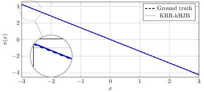
(a) S1, where $\pi_{\infty}^{\star}(x)=-\sqrt{2}x$

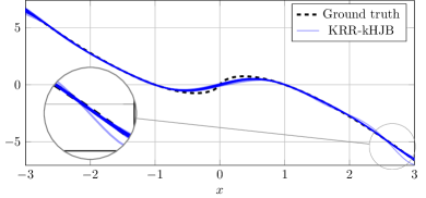
(b) S2, where $\pi_{\infty}^{\star}(x)=-\ln{(x^{2})}x$

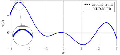
(c) S3, where $\pi_{\infty}^{\star}(x)=\frac{1}{2}+\sin{(2x)}x$

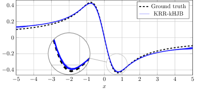
(d) S4, where $\pi_{\infty}^{\star}(x)=x^{3}-x\sqrt{1+x^{4}}$

Figure 1: Performance with 50 independent KRR estimations for different systems with various nonlinearities. The optimal control laws $\pi_{\infty}^{\star}$ for $\ell(x,u)=x^{2}+u^{2}$ are unknown to the algorithm, but used by us as ground truth. Our proposed data-driven kernel HJB approach recovers these optimal control laws reliably and exhibits little variance w.r.t. to different i.i.d. draws from the data distribution.

V Implementation and Numerical Examples

In this experimental section, we present numerical examples to evaluate the accuracy of the data-driven generated global optimal control law using Algorithm. 1. We discuss implementation details and apply the proposed method to challenging benchmark examples, which are implemented in JULIA 1.10.1.

V-A Implementation Details

Our numerical examples are based on Gaussian Radial Basis Function (RBF) kernels of the form

$$k(\bm{x},\bm{y}) = \exp{\left(\textstyle-\frac{\|\bm{x}-\bm{y}\|^{2}}{\sigma^{2}}\right)}$$

$$\text{and}\quad{}^{\epsilon}\!k(\bm{x},\bm{y}) = \textstyle\frac{\sigma}{\sqrt{\sigma^{2}+2\epsilon{\Delta t}}}\exp{\left(-\frac{\|\bm{x}-\bm{y}\|^{2}}{\sigma^{2}+2\epsilon{\Delta t}}\right)}.$$

While the first kernel is used to compute the control-tensorized Gram matrix in Algorithm 1, the Euler-Maruyama cross-covariance can be computed by evaluating its associated diffusion by using the above explicit expression for ${}^{\epsilon}\!k$. Additionally, we set $\gamma=10^{-8}$ and $\epsilon=0.02$. The RBF scale $\sigma$ is tuned separately for each benchmark, using a grid search based on the evaluation criteria outlined in Section IV-F. The data matrices are generated using a uniform random scalar input $\bm{u}$ on the domain $\mathbb{U}_{\mathrm{S}}=[-1,1]$.

V-B Benchmark Problems

V-B1 1D Benchmark Collection

Let us consider the open-loop controlled scalar system $\dot{x}=f(x)+G(x)u$ with input $u\in\mathbb{R}$. For $f(x)=-\frac{1}{2}x\left(1-G(x)^{2}\right)$ and stage cost functional ${\ell}(x,u)=x^{2}+u^{2}$, the globally optimal feedback control law is known and given by ${\pi}^{\star}_{\infty}(x)=-G(x)x$ [17]. We implement three different instances of $G(x)$, listed as Systems S1, S2 and S3 in Table III. For example, System S1 is an open-loop unstable linear system, but our data-driven method neither knows about the linearity of this problem nor has any prior information about its stabilizability. Additionally, we implement another nonlinear system, System S4, for which the optimal control law has a known closed-form solution [22]. The dynamics are given by $\dot{x}=-x^{3}+u$. This problem has the globally optimal feedback control law $\pi_{\infty}^{\star}(x)=x^{3}-x\sqrt{1+x^{4}}$.

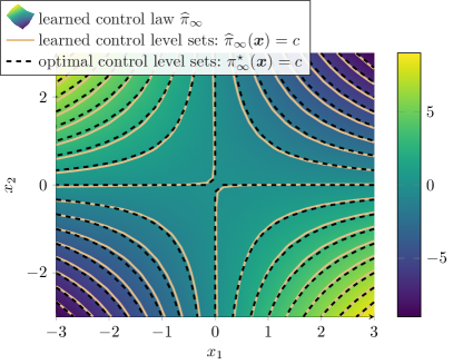
Figure 2: Contours of the learned optimal controller for the Van der Pol system with a linearly uncontrollable origin and unstable limit cycle, compared to the known optimal feedback law $\pi_{\infty}^{\star}(\bm{x})=-x_{1}x_{2}$.

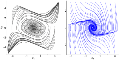
Figure 3: Taming an unstable limit cycling system with linearily uncontrollable origin. Left: Open loop $(u{=}0)$ of the original system. Right: Closed loop under our learned control law for the stage cost function $l(\bm{x}){=}x^{2}_{2}$.

System (${\mathbb{X}}_{S},{\Delta t}$)	$G(x)$	$f(x)$
S1 $\left([-3,3],10^{-2}\right)$	$\sqrt{2}$	$\frac{1}{2}x$
S2 $\left([-3,3],10^{-3}\right)$	$\ln{(x^{2})}$	$-\frac{1}{2}x(1-\ln{(x^{2})}^{2})$
S3 $\left([-3,3],10^{-3}\right)$	$\frac{1}{2}+\sin{(2x)}$	$-\frac{3}{8}x+\frac{1}{2}x\sin{(2x)}+\frac{1}{2}x\sin{(2x)}^{2}$
S4 $\left([-5,5],10^{-2}\right)$	$1$	$-x^{3}$

TABLE III: 1D Benchmark examples. Definitions of $f$ and $G$ with the respective domain ${\mathbb{X}}_{S}$ and sampling time ${\Delta t}$ used to generate the training samples.

The systems, along with their respective domains and sampling times, are detailed in Table III. We generate 50 independent KRR estimations for Systems S1, S2, and S3 using $N=1000$ training points each, and for System S4 using $N=400$ training points. For a sampling time of ${\Delta t}=10^{-3}$s, the recursion of Algorithm 1 is executed for $H=5000$ steps. In comparison, for a sampling time of ${\Delta t}=10^{-2}$s, only $H=500$ steps are taken to ensure the convergence of the value function. Figure 1 illustrates a comparison between the control laws derived from the value function recursion in Algorithm 1 and the known optimal control laws. Additionally, Table IV presents the mean and standard deviation of the Root Mean Square Error (RMSE) $\sqrt{\frac{\sum_{i=1}^{N}(\widehat{\pi}_{\infty}^{\star}(\bm{x}^{(i)})-\pi_{\infty}^{\star}(\bm{x}^{(i)}))^{2}}{N}}$ between our estimated control laws and the ground truth optimal control laws.

System	RBF Scale $\sigma$	rmse (mean)	rmse (std)
S1	$1.2$	$1.29\times 10^{-2}$	$1.59\times 10^{-3}$
S2	$1.8$	$1.31\times 10^{-1}$	$1.53\times 10^{-1}$
S3	$2$	$2.17\times 10^{-2}$	$8.13\times 10^{-3}$
S4	$1$	$1.91\times 10^{-2}$	$2.94\times 10^{-4}$

TABLE IV: 1D Benchmark examples: rmse of the obtained control law versus the ground-truth control law, evaluated on $100$ test data points.

V-B2 Unstable oscillator

Consider a Van der Pol oscillator system $\dot{x}_{1}=x_{2}$, $\dot{x}_{2}=-x_{1}-\frac{1}{2}x_{2}\left(1-{x_{1}}^{2}\right)+x_{1}u$ for stage cost ${\ell}(\bm{x},u)=\frac{1}{2}(x_{2}^{2}+u^{2})$. This particular example admits an explicit solution of the Hamilton-Jacob-Bellman equations, for which the globally optimal feedback law is given by $\pi_{\infty}^{\star}(\bm{x})=-x_{1}x_{2}$ [61]. Notice that this system has a linearly uncontrollable equilibrium at $(0,0)^{\top}$ and an unstable limit cycle (Fig. 3, left). In this example, the training dataset is sampled from a grid of initial conditions within the limits $|x_{1}|\leq 3$ and $|x_{2}|\leq 3$, with $N=2500$ training points for the KRR estimation. We identified $\sigma=20$ as a near-optimal RBF scale. Fig. 2 shows that the approximated feedback law closely relates to the globally optimal feedback law $\pi_{\infty}^{\star}(\bm{x})$. This is verified by the relatively low RMSE ($7.24\times 10^{-2}$) between the approximated feedback law $\widehat{\pi}_{\infty}^{\star}(\bm{x})$ and the known globally optimal feedback law $\pi_{\infty}^{\star}(\bm{x})$, computed over a grid of 900 test points $(x_{1},x_{2})\in[-3,3]\times[-3,3]$. With the defined cost functional, the closed-loop system under the approximated feedback law now exhibits an asymptotically stable origin, as illustrated in the right panel of Fig. 3.

VI Conclusion

This paper has presented a groundbreaking fully data-driven framework for approximating optimal feedback laws in stochastic optimal control problems with unknown dynamics and stage costs (cf. Table I). By leveraging the power of kernel mean embedding operators and the kernel trick, we develop a novel Kernel HJB recursion that breaks the curse of dimensionality in traditional dynamic programming and leads to time- and sample-complexity that is effectively independent of state dimensionality. Our system identification procedure scales linearly with states and controls, enabling polynomial runtime complexity of both the identification as well as control, as summarized in Table II. Furthermore, our theoretical analysis from Theorem 3 has established statistical convergence rate guarantees for the value function approximation, achieved without relying on any system prior knowledge.

This work’s novel algorithmic framework follows from rigorous theoretical foundations and is well-supported by numerical experiments. The Kernel HJB recursion and operator-theoretic system identification offer a promising avenue for addressing high-dimensional and uncertain optimal control problems. This versatility opens a variety of future research directions, including large-scale regression via data-efficient low-rank estimators and feature spaces for further reduction of the computational complexity of the proposed algorithms.

References

• [1] N. Aronszajn. Theory of reproducing kernels. Trans. Am. Math. Soc., 68(3):337, 1950.
• [2] Francis Bach. On the equivalence between kernel quadrature rules and random feature expansions. J. Mach. Learn. Res., 18(21):1–38, 2017.
• [3] P.L Bartlett and S. Mendelson. Rademacher and gaussian complexities: Risk bounds and structural results. Technical report, 2002.
• [4] R.E. Bellman. Dynamic Programming. Princeton University Press, 1957.
• [5] A. Berlinet and C. Thomas-Agnan. Reproducing Kernel Hilbert Spaces in Probability and Statistics. Springer US, Boston, MA, 2004.
• [6] P. Bevanda, M. Beier, A. Lederer, S. Sosnowski, E. Hüllermeier, and S. Hirche. Koopman kernel regression. In NeurIPS, volume 37, 2023.
• [7] P. Bevanda, B. Driessen, L.C. Iacob, R. Toth, S. Sosnowski, and S. Hirche. Nonparametric control-koopman operator learning: Flexible and scalable models for prediction and control. arXiv:2405.07312, 2024.
• [8] P. Bevanda, S. Sosnowski, and S. Hirche. Koopman operator dynamical models: Learning, analysis and control. Annu. Rev. Control, 52:197–212, 2021.
• [9] L.T. Biegler. An overview of simultaneous strategies for dynamic optimization. Chem. Eng. Process. Process Intensif., 46:1043–1053, 2007.
• [10] H.G. Bock and K.J. Plitt. A multiple shooting algorithm for direct solution of optimal control problems. Proceedings 9th IFAC World Congress Budapest, pages 243–247, 1984.
• [11] V.I. Bogachev, N.V. Krylov, M. Röckner, and S.V. Shaposhnikov. Fokker-Planck-Kolmogorov equations. AMS, 2015.
• [12] S. Brenner and R.L. Scott. The mathematical theory of finite element methods. Springer, 2005.
• [13] E. Caldarelli, A. Chatalic, A. Colome, C. Molinari, C. Ocampo-Martinez, C. Torras, and L. Rosasco. Linear quadratic control of nonlinear systems with Koopman operator learning and the Nyström method. arXiv:2403.02811v1, 2024.
• [14] M.G. Crandall, H. Ishii, and P.-L. Lions. User’s guide to viscosity solutions of second order partial differential equations. Bull. Am. Math. Soc., 27(1):1–67, 1992.
• [15] E. De Vito, N. Mücke, and L. Rosasco. Reproducing kernel Hilbert spaces on manifolds: Sobolev and diffusion spaces. Analysis and Applications, 19:363–396, May 2021.
• [16] F. Dörfler, M. Chertkov, and F. Bullo. Synchronization in complex oscillator networks and smart grids. Proc. Natl. Acad. Sci. U.S.A., 110(6):2005–2010, 2013.
• [17] J. Doyle, J.A. Primbs, B. Shapiro, and V. Nevistic. Nonlinear games: examples and counterexamples. In Proc. IEEE Conf. Decis. Control, volume 4, pages 3915–3920 vol.4, 1996.
• [18] L. Elsner and M. Paardekooper. On measures of nonnormality of matrices. Linear Algebra Appl., 92:107–123, 1987.
• [19] W.H. Fleming and H.M. Soner. Controlled Markov Processes and Viscosity Solutions. Springer, 1993.
• [20] A.D. Fokker. Die mittlere Energie rotierender elektrischer Dipole im Strahlungsfeld. Annalen der Physik, 4(3):810–820, 1914.
• [21] S. Grünewälder, G. Lever, L. Baldassarre, S. Patterson, A. Gretton, and M. Pontil. Conditional mean embeddings as regressors. In ICML, pages 1823–1830, New York, NY, USA, 2012. Omnipress.
• [22] Y. Guo, B. Houska, and M.E. Villanueva. A tutorial on Pontryagin-Koopman operators for infinite horizon optimal control. In Proc. IEEE Conf. Decis. Control, pages 6800–6805, 2022.
• [23] R.Z. Has’minskiǐ. Ergodic properties of recurrent diffusion processes and stabilization of the solution of the Cauchy problem for parabolic equations. Theory Probab. Appl., 5:179–196, 1960.
• [24] P. Henrici. Bounds for iterates, inverses, spectral variation and fields of values of non-normal matrices. Numerische Mathematik, 4:24–40, 1962.
• [25] J. Hespanha and K. Çamsarı. Markov chain Monte Carlo for Koopman-based optimal control. IEEE Control Syst. Lett, 8:1901–1906, 2024.
• [26] M. Hinze, R. Pinnau, M. Ulbrich, and S. Ulbrich. Optimization with PDE Constraints. Springer, 2009.
• [27] B. Houska. Convex operator-theoretic methods in stochastic control. http://arxiv.org/abs/2305.17628, May 2023.
• [28] M. Ibrahim, C. Kallies, and R. Findeisen. Learning-supported approximated optimal control for autonomous vehicles in the presence of state dependent uncertainties. In Proc. Eur. Control Conf., pages 338–343, 2020.
• [29] P. Inzerili, C. Kostić, K. Lounici, P. Novelli, and M. Pontil. Consistent long-term forecasting of ergodic dynamical systems, 2024.
• [30] S. Klus, I. Schuster, and K. Muandet. Eigendecompositions of transfer operators in reproducing kernel hilbert spaces. J. Nonlinear Sci., 30:283–315, February 2020.
• [31] A.N. Kolmogoroff. Über die analytischen Methoden in der Wahrscheinlichkeitsrechnung. Mathematische Annalen, 104:415–458, 1931.
• [32] B.O. Koopman. Hamiltonian systems and transformations in Hilbert space. Proc. Natl. Acad. Sci. U.S.A., 17(5):315–318, 1931.
• [33] B.O. Koopman and J. von Neumann. Dynamical systems of continuous spectra. Proc. Natl. Acad. Sci. U.S.A., 18(3), 1932.
• [34] M. Korda and I. Mezić. Linear predictors for nonlinear dynamical systems: Koopman operator meets model predictive control. Automatica, 93:149–160, 2018.
• [35] V. Kostic, K. Lounici, P. Novelli, and M. Pontil. Sharp spectral rates for Koopman operator learning. In NeurIPS, volume 36, pages 32328–32339, 2023.
• [36] V. Kostic, P. Novelli, R. Grazzi, K. Lounici, and M. Pontil. Learning invariant representations of time-homogeneous stochastic dynamical systems. In ICLR 2024, 2024.
• [37] V. Kostic, P. Novelli, A. Maurer, C. Ciliberto, L. Rosasco, and M. Pontil. Learning dynamical systems via Koopman operator regression in Reproducing Kernel Hilbert Spaces. In NeurIPS, pages 4017–4031, 2022.
• [38] I. Koutsopoulos and L. Tassiulas. Optimal control policies for power demand scheduling in the smart grid. IEEE J. Sel. Areas Commun., 30(6):1049–1060, 2012.
• [39] N.V. Krylov. Controlled diffusion processes. Springer, 2008.
• [40] V. Kumar, E. Todorov, and S. Levine. Optimal control with learned local models: Application to dexterous manipulation. In IEEE In. Conf. Robot. Autom., pages 378–383. IEEE, 2016.
• [41] Zhu Li, Dimitri Meunier, Mattes Mollenhauer, and Arthur Gretton. Optimal rates for regularized conditional mean embedding learning. In NeurIPS, volume 35, pages 4433–4445, 2022.
• [42] L. Lindemann, M. Cleaveland, G. Shim, and G. Pappas. Safe planning in dynamic environments using conformal prediction. IEEE Robot. Automat. Lett., 8:5116–5123, August 2023.
• [43] X. Liu. Fuel-optimal rocket landing with aerodynamic controls. J. Guid. Control Dyn., 42(1):65–77, 2019.
• [44] X. Liu, Z. Liu, and P. Huang. Stochastic optimal control for robot manipulation skill learning under time-varying uncertain environment. IEEE Trans. Cybern., 54(4):2015–2025, 2022.
• [45] Y. Meng, R. Zhou, A. Mukherjee, M. Fitzsimmons, C. Song, and J. Liu. Physics-informed neural network policy iteration: Algorithms, convergence, and verification. February 2024.
• [46] J. Mercer. Functions of positive and negative type, and their connection the theory of integral equations. Philos. Trans. R. Soc. London, Ser. A, 209(441-458):415–446, January 1909.
• [47] I. Mezić. Spectral properties of dynamical systems, model reduction and decompositions. Nonlinear Dynamics, 41(1–3):309–325, 2005.
• [48] J. Moyalan, H. Choi, Y. Chen, and Vaidya U. Data-driven optimal control via linear transfer operators: A convex approach. Automatica, 150:110841, 2023.
• [49] K. Muandet, K. Fukumizu, B. Sriperumbudur, and B. Schölkopf. Kernel mean embedding of distributions: A review and beyond. Found. Trends Mach. Learn., 10(1-2):1–141, 2017.
• [50] B. Oksendal. Stochastic Differential Equations. Springer, 2000.
• [51] Guanru Pan, Ruchuan Ou, and Timm Faulwasser. On a stochastic fundamental lemma and its use for data-driven optimal control. IEEE Trans. Autom. Control, 68(10):5922–5937, 2023.
• [52] M. Planck. Über einen Satz der statistischen Dynamik und seine Erweiterung in der Quantentheorie. Sitzungsber. K. Preuss. Akad. Wiss, pages 324–341, 1917.
• [53] E. Platen. An introduction to numerical methods for stochastic differential equations. Acta Numerica, 8:197–246, 1999.
• [54] B.K. Poolla, S. Bolognani, and F. Dörfler. Optimal placement of virtual inertia in power grids. IEEE Trans. Autom. Control, 62(12):6209–6220, 2017.
• [55] M.L. Puterman. Optimal control of diffusion processes with reflection. J. Optim. Theory Appl., 22(1), 1977.
• [56] A. Rudi, L. Carratino, and L. Rosasco. FALKON: An optimal large scale kernel method. NeurIPS, 29, 2017.
• [57] Charis Stamouli, Evangelos Chatzipantazis, and George J. Pappas. Structural Risk Minimization for Learning Nonlinear Dynamics. arXiv e-prints, 2023.
• [58] I. Steinwart and A. Christmann. Support Vector Machines. Information Science and Statistics. Springer, New York, NY, first edition, 2008.
• [59] M. Talagrand and M. Ledoux. Probability in Banach Spaces. Springer-Verlag, New York, 1991.
• [60] U. Vaidya and D. Tellez-Castro. Data-driven stochastic optimal control with safety constraints using linear transfer operators. IEEE Trans. Autom. Control, 69(4):2100–2115, 2024.
• [61] M.E. Villanueva, C.N. Jones, and B. Houska. Towards global optimal control via Koopman lifts. Automatica, 132(109610), 2021.
• [62] R. Vinter. Convex duality and nonlinear optimal control. SIAM J. Control Optim., 31(2):518–538, 1993.
• [63] W.M. Wonham. Liapunov criteria for weak stochastic stability. J. Differ. Equations, 2:195–207, 1966.