Optimal parameter choice for regularized Shannon sampling formulas

Abstract

The fast reconstruction of a bandlimited function from its sample data is an essential problem in signal processing. In this paper, we consider the widely used Gaussian regularized Shannon sampling formula in comparison to regularized Shannon sampling formulas employing alternative window functions, including the modified Gaussian function, the $\sinh$-type window function, and the continuous Kaiser–Bessel window function. It is shown that the approximation errors of these regularized Shannon sampling formulas possess an exponential decay with respect to the truncation parameter. The main focus of this paper is to identify the optimal variance of the (modified) Gaussian function as well as the optimal shape parameters of the $\sinh$-type window function and the continuous Kaiser–Bessel window function, with the aim of achieving the fastest exponential decay of the approximation error. In doing so, we demonstrate that the decay rate of the $\sinh$-type regularized Shannon sampling formula is considerably superior to that of the Gaussian regularized Shannon sampling formula. Additionally, numerical experiments illustrate the theoretical results.

Key words: Shannon sampling series, optimal regularization, bandlimited function, approximation error, exponential decay, Gaussian regularized Shannon sampling formulas, $\sinh$-type regularized Shannon sampling formulas.

AMS Subject Classifications: 62D05, 42A10, 41A25, 94A20.

1 Introduction

In signal processing, the fast reconstruction of a bandlimited function from its sample data is of fundamental importance. A function $f\in L^{2}(\mathbb{R})\cap C(\mathbb{R})$ is called bandlimited with bandwidth $\delta>0$, if its Fourier transform

$$({\mathcal{F}}f)(\omega)={\hat{f}}(\omega)\coloneqq\frac{1}{\sqrt{2\pi}}\,\int_{\mathbb{R}}f(t)\,{\mathrm{e}}^{-{\mathrm{i}}t\omega}\,{\mathrm{d}}t\,,\quad\omega\in\mathbb{R}\,,$$ (1.1)

vanishes for all $|\omega|\geq\delta$. For such a bandlimited function with $\delta\in(0,\,\pi]$ the famous Shannon sampling theorem, see [31, 14, 28], states that

$$f(t)=\sum_{k\in\mathbb{Z}}f(k)\,\mathrm{sinc}(t-k)\,,\quad t\in\mathbb{R}\,,$$ (1.2)

where

$$\mathrm{sinc}(t)\coloneqq\begin{cases}\frac{\sin(\pi t)}{\pi t}&\colon t\in\mathbb{R}\setminus\{0\}\,,\\ 1&\colon t=0\,,\end{cases}$$ (1.3)

denotes the cardinal sine function. It is known that the Shannon sampling series (1.2) converges absolutely and uniformly on whole $\mathbb{R}$. However, the practical use of (1.2) is limited, since its evaluation requires infinitely many samples and its truncated version is not a good approximation due to the slow decay of the cardinal sine function, see [11]. In addition to this rather poor convergence, it is known, see [8, 9, 7], that in the presence of noise in the samples $f(k)$, $k\in\mathbb{Z}$, of a bandlimited function $f\in L^{2}(\mathbb{R})\cap C(\mathbb{R})$ the convergence of Shannon sampling series (1.2) may even break down completely. Therefore, it was proposed to consider the regularization of the Shannon sampling series with a suitable window function. Note that many authors such as [6, 17, 26, 19, 29] used window functions in the frequency domain, but the recent study [13] has shown that it is much more beneficial to employ a window function in the spatial domain, cf. [22, 23, 29, 16, 15, 5, 12]. In the following, a window function $\varphi:\,\mathbb{R}\to[0,\,1]$ is an even function in $L^{2}(\mathbb{R})\cap C(\mathbb{R})$ which decreases on $[0,\,\infty)$ and fulfills $\varphi(0)=1$. By ${\mathbf{1}}_{[-m,\,m]}$ we denote the characteristic function of the interval $[-m,\,m]$ with $m\in\mathbb{N}\setminus\{1\}$, i. e., the function

$${\mathbf{1}}_{[-m,\,m]}(t)\coloneqq\begin{cases}1&\colon t\in[-m,\,m]\,,\\ 0&\colon t\in\mathbb{R}\setminus[-m,\,m]\,.\end{cases}$$

In this paper, we assume that the bandwidth $\delta$ of $f$ fulfills the so-called oversampling condition $0<\delta<\pi$. Then we recover $f$ by the $\varphi$-regularized Shannon sampling formula

$$\big{(}R_{\varphi,m}f\big{)}(t)\coloneqq\sum_{k\in\mathbb{Z}}f(k)\,\mathrm{sinc}(t-k)\,\varphi(t-k)\,{\mathbf{1}}_{[-m,\,m]}(t-k)\,,\quad t\in\mathbb{R}\,,$$ (1.4)

where $m\in\mathbb{N}\setminus\{1\}$ is the so-called truncation parameter. In doing so, we consider the following window functions $\varphi:\,\mathbb{R}\to[0,\,1]$.

Example 1.1.

The most popular window function, see e. g. [22, 25, 27, 30, 15, 5], is the Gaussian function

$$\varphi_{\mathrm{Gauss}}(t)\coloneqq\mathrm{e}^{-t^{2}/(2\sigma^{2})}\,,\quad t\in\mathbb{R}\,,$$ (1.5)

with variance $\sigma^{2}>0$. In addition, [25, 24] considered the modified Gaussian function

$$\varphi_{\mathrm{modGauss}}(t)\coloneqq\mathrm{e}^{-t^{2}/(2\sigma^{2})}\,\cos(\lambda t)\,,\quad t\in\mathbb{R}\,,$$ (1.6)

with the parameters $\sigma^{2}>0$ and $\lambda\geq 0$. Then the corresponding expression (1.4) is named the (modified) Gaussian regularized Shannon sampling formula. Note that these two window functions (1.5) and (1.6) are supported on whole $\mathbb{R}$.

Here we prefer window functions which are compactly supported on the interval $[-m,\,m]$, as studied in [12, 13]. The $\sinh$-type window function is defined as

$$\varphi_{\sinh}(t)\coloneqq\begin{cases}\frac{1}{\sinh\beta}\,\sinh\Big{(}\beta\,\sqrt{1-\tfrac{t^{2}}{m^{2}}}\,\Big{)}&\colon t\in[-m,\,m]\,,\\ 0&\colon t\in\mathbb{R}\setminus[-m,\,m]\,,\end{cases}$$ (1.7)

with shape parameter $\beta>0$, see [21]. Then the corresponding expression (1.4) is termed the $\sinh$-type regularized Shannon sampling formula. The continuous Kaiser–Bessel window function is defined as

$$\varphi_{\mathrm{cKB}}(t)\coloneqq\begin{cases}\frac{1}{I_{0}(\beta)-1}\,\big{(}I_{0}(\beta\sqrt{1-t^{2}/m^{2}})-1\big{)}&\colon t\in[-m,\,m]\,,\\ 0&\colon t\in\mathbb{R}\setminus[-m,\,m]\,,\end{cases}$$ (1.8)

with convenient shape parameter $\beta>0$, see [21]. Then the corresponding expression (1.4) is called the continuous Kaiser–Bessel regularized Shannon sampling formula. We remark that these two window functions (1.7) and (1.8) are well-studied in the context of the nonuniform fast Fourier transform (NFFT), see e. g. [20, Section 6] and [4, 3].       

Due to the definition of the cardinal sine function (1.3) we have $\mathrm{sinc}(n-k)=\delta_{n,k}$ and therefore the regularized Shannon sampling formula $R_{\varphi,m}f$ in (1.4) has the interpolation property

$$\big{(}R_{\varphi,m}f\big{)}(n)=f(n)\,,\quad n\in\mathbb{Z}\,.$$ (1.9)

Moreover, the use of the characteristic function ${\mathbf{1}}_{[-m,\,m]}$ in (1.4) leads to localized sampling of $f$, i. e., the computation of $\big{(}R_{\varphi,m}f\big{)}(t)$ for any $t\in\mathbb{R}\setminus\mathbb{Z}$ requires only $2m$ samples $f(k)$, where $k\in\mathbb{Z}$ fulfills the condition $|k-t|\leq m$. Especially, for $t\in(0,\,1)$ we obtain the finite sum

$$\big{(}R_{\varphi,m}f\big{)}(t)=\sum_{k=1-m}^{m}f(k)\,\mathrm{sinc}(t-k)\,\varphi(t-k)\,.$$

As in many applications, we use oversampling of the given bandlimited function $f$ with bandwidth $\delta<\pi$, i. e., the function $f$ is sampled on the integer grid $\mathbb{Z}$.

In this paper, we focus on the $\varphi$-regularized Shannon sampling formulas (1.4) for the window functions $\varphi$ given in Example 1.1. To compare the corresponding approaches, we present estimates on the uniform approximation error

$$\|f-R_{\varphi,m}f\|_{C_{0}(\mathbb{R})}\coloneqq\max_{t\in\mathbb{R}}\big{|}f(t)-\big{(}R_{\varphi,m}f\big{)}(t)\big{|}\,,$$ (1.10)

where $C_{0}(\mathbb{R})$ denotes the Banach space of continuous functions $g\colon\!\mathbb{R}\to\mathbb{C}$ vanishing as $|t|\to\infty$. The main focus of this paper is to find the optimal variance $\sigma^{2}$ of the (modified) Gaussian window function (1.5) and (1.6), respectively, as well as the optimal shape parameter $\beta$ of the $\sinh$-type window function (1.7) and the continuous Kaiser–Bessel window function (1.8), such that the exponential decay of the approximation error (1.10) is the fastest.

For this purpose, we initially study the uniform approximation error of general $\varphi$-regularized Shannon sampling formulas (1.4) in Section 2. Afterwards, we specify our findings for the window functions $\varphi$ introduced in Example 1.1. In particular, Section 3 deals with the (modified) Gaussian window function (1.5) and (1.6), respectively, while Section 4 is concerned with the $\sinh$-type window function (1.7) and Section 5 with the continuous Kaiser–Bessel window function (1.8).

2 Approximation error of regularized Shannon sampling formulas

First we estimate the uniform approximation error of the $\varphi$-regularized Shannon sampling formula (1.4), analogous to [12, Theorem 3.2] and [13, Theorem 4.1].

Theorem 2.1.

Assume that $f\in L^{2}(\mathbb{R})\cap C(\mathbb{R})$ is bandlimited with bandwidth $\delta\in(0,\,\pi)$. Further let $\varphi:\,\mathbb{R}\to[0,\,1]$ be an even function in $L^{2}(\mathbb{R})\cap C(\mathbb{R})$ which is decreasing on $[0,\,\infty)$ with $\varphi(0)=1$, and let $m\in{\mathbb{N}}\setminus\{1\}$ be given.
Then the $\varphi$-regularized Shannon sampling formula (1.4) satisfies the error estimate

$$\|f-R_{\varphi,m}f\|_{C_{0}(\mathbb{R})}\leq\big{(}E_{1}(m)+E_{2}(m)\big{)}\,\|f\|_{L^{2}(\mathbb{R})}\,,\quad m\in\mathbb{N}\setminus\{1\}\,,$$

with the error constants

$$E_{1}(m) \coloneqq\max_{\omega\in[-\delta,\,\delta]}\bigg{|}1-\frac{1}{\sqrt{2\pi}}\,\int_{\omega-\pi}^{\omega+\pi}{\hat{\varphi}}(\tau)\,{\mathrm{d}}\tau\,\bigg{|}\,,$$ (2.1)

$$E_{2}(m) \coloneqq\frac{\sqrt{2}}{\pi\,m}\,\sqrt{\varphi^{2}(m)+\int_{m}^{\infty}\varphi^{2}(t)\,\mathrm{d}t}\,.$$ (2.2)

Proof. (i) Initially, we consider only the case $t\in(0,\,1)$, where we split the approximation error

$$f(t)-\big{(}R_{\varphi,m}f\big{)}(t)=e_{1}(t)+e_{2,0}(t)\,,\quad t\in(0,\,1)\,,$$

into the regularization error

$$e_{1}(t)\coloneqq f(t)-\sum_{k\in\mathbb{Z}}f(k)\,\mathrm{sinc}(t-k)\,\varphi(t-k)\,,\quad t\in\mathbb{R}\,,$$ (2.3)

and the truncation error

$$e_{2,0}(t) \coloneqq\sum_{k\in\mathbb{Z}}f(k)\,\mathrm{sinc}(t-k)\,\varphi(t-k)-\big{(}R_{\varphi,m}f\big{)}(t)$$

$$=\sum_{k\in\mathbb{Z}\setminus\{1-m,\ldots,m\}}f(k)\,\mathrm{sinc}(t-k)\,\varphi(t-k)\,,\quad t\in(0,\,1)\,.$$ (2.4)

(ii) To estimate the regularization error (2.3), we start our study by considering the Fourier transform (1.1) of the function $\varphi\,\mathrm{sinc}$, i. e., the term

$${\mathcal{F}}(\varphi\,\mathrm{sinc})(\omega)=\frac{1}{\sqrt{2\pi}}\,\int_{\mathbb{R}}\varphi(t)\,\mathrm{sinc}(t)\,\mathrm{e}^{-\mathrm{i}\omega t}\,\mathrm{d}t\,.$$

Using the convolution property of $\mathcal{F}$ in $L^{2}(\mathbb{R})$ (see [20, Theorem 2.26]), we have

$${\mathcal{F}}(\varphi\,\mathrm{sinc})(\omega)=\big{(}{\hat{\varphi}}\star({\mathcal{F}}\mathrm{sinc})\big{)}(\omega)=\frac{1}{\sqrt{2\pi}}\,\int_{\mathbb{R}}\hat{\varphi}(\omega-\tau)\,(\mathcal{F}\mathrm{sinc})(\tau)\,\mathrm{d}\tau\,,$$

and hence by

$$(\mathcal{F}\mathrm{sinc})(\tau)=\frac{1}{\sqrt{2\pi}}\,{\mathbf{1}}_{[-\pi,\pi]}(\tau)$$

we obtain

$${\mathcal{F}}(\varphi\,\mathrm{sinc})(\omega)=\frac{1}{2\pi}\,\int_{\omega-\pi}^{\omega+\pi}\hat{\varphi}(\tau)\,\,\mathrm{d}\tau\,.$$

Consequently, using the shifting property of $\mathcal{F}$, the Fourier transform (1.1) of the shifted function $\varphi(t-k)\,\mathrm{sinc}(t-k)$ with $k\in\mathbb{Z}$ reads as

$$\frac{1}{\sqrt{2\pi}}\,\int_{\mathbb{R}}\varphi(t-k)\,\mathrm{sinc}(t-k)\,\mathrm{e}^{-\mathrm{i}\omega t}\,\mathrm{d}t=\mathrm{e}^{-\mathrm{i}\omega k}\,{\mathcal{F}}(\varphi\,\mathrm{sinc})(\omega)=\frac{1}{2\pi}\,\mathrm{e}^{-\mathrm{i}\omega k}\,\int_{\omega-\pi}^{\omega+\pi}\hat{\varphi}(\tau)\,\,\mathrm{d}\tau\,.$$

Therefore, the Fourier transform of the regularization error $e_{1}$ in (2.3) has the form

$${\hat{e}}_{1}(\omega)={\hat{f}}(\omega)-\bigg{(}\frac{1}{2\pi}\,\sum_{k\in\mathbb{Z}}f(k)\,\mathrm{e}^{-\mathrm{i}\omega k}\bigg{)}\,\int_{\omega-\pi}^{\omega+\pi}\hat{\varphi}(\tau)\,\,\mathrm{d}\tau\,.$$ (2.5)

Note that since the set of shifted cardinal sine functions $\mathrm{sinc}(\cdot-k)$ with $k\in\mathbb{Z}$ forms an orthonormal system in $L^{2}(\mathbb{R})$, i. e.

$$\int_{\mathbb{R}}\mathrm{sinc}(t-k)\,\mathrm{sinc}(t-\ell)\,\mathrm{d}t=\delta_{k,\ell}\,,\quad k,\,\ell\in\mathbb{Z}\,,$$

and the given function $f$ can be represented by the Shannon sampling series (1.2), we obtain that

$$\sum_{k\in\mathbb{Z}}|f(k)|^{2} =\sum_{k\in\mathbb{Z}}\sum_{\ell\in\mathbb{Z}}f(k)\,\overline{f(\ell)}\int_{\mathbb{R}}\mathrm{sinc}(t-k)\,\mathrm{sinc}(t-\ell)\,\mathrm{d}t$$

$$=\int_{\mathbb{R}}f(t)\,\overline{f(t)}\,\mathrm{d}t=\|f\|_{L^{2}(\mathbb{R})}^{2}<\infty\,,$$ (2.6)

and thus the series

$$\sum_{k\in\mathbb{Z}}f(k)\,{\mathrm{e}}^{-{\mathrm{i}}\omega k}$$

converges in $L^{2}([-\pi,\pi])$. Moreover, since $f$ is bandlimited with bandwidth $\delta\in(0,\,\pi)$, we have ${\hat{f}}(\omega)=0$ for all $\omega\in\mathbb{R}\setminus[-\delta,\,\delta]$, and thereby the restricted function $\hat{f}\big{|}_{[-\pi,\,\pi]}$ belongs to $L^{2}([-\pi,\pi])$. Hence, this restricted function possesses the $2\pi$-periodic Fourier expansion

$${\hat{f}}(\omega)=\sum_{k\in\mathbb{Z}}c_{k}(\hat{f})\,\mathrm{e}^{-\mathrm{i}\omega k}\,,\quad\omega\in[-\pi,\,\pi]\,,$$

with the Fourier coefficients

$$c_{k}(\hat{f}) =\frac{1}{2\pi}\,\int_{-\pi}^{\pi}{\hat{f}}(\tau)\,\mathrm{e}^{\mathrm{i}k\tau}\,\mathrm{d}\tau=\frac{1}{2\pi}\,\int_{\mathbb{R}}{\hat{f}}(\tau)\,\mathrm{e}^{\mathrm{i}k\tau}\,\mathrm{d}\tau=\frac{1}{\sqrt{2\pi}}\,f(k)\,,\quad k\in\mathbb{Z}\,,$$

by inverse Fourier transform. In other words, the function $\hat{f}$ can be represented in the form

$$\hat{f}(\omega)={\hat{f}}(\omega)\,{\mathbf{1}}_{[-\delta,\delta]}(\omega)=\frac{1}{\sqrt{2\pi}}\,\bigg{(}\sum_{k\in\mathbb{Z}}f(k)\,\mathrm{e}^{-\mathrm{i}k\omega}\bigg{)}\,{\mathbf{1}}_{[-\delta,\delta]}(\omega)\,,\quad\omega\in\mathbb{R}\,.$$ (2.7)

Introducing the auxiliary function

$$\Delta_{\varphi}(\omega)\coloneqq{\mathbf{1}}_{[-\delta,\delta]}(\omega)-\frac{1}{\sqrt{2\pi}}\,\int_{\omega-\pi}^{\omega+\pi}\hat{\varphi}(\tau)\,\,\mathrm{d}\tau\,,\quad\omega\in\mathbb{R}\,,$$

we see by inserting (2.7) into (2.5) that

$${\hat{e}}_{1}(\omega)={\hat{f}}(\omega)\,\Delta_{\varphi}(\omega)\,,\quad\omega\in\mathbb{R}\,,$$

and thereby

$$\big{|}{\hat{e}}_{1}(\omega)\big{|}=\big{|}{\hat{f}}(\omega)\big{|}\,\big{|}\Delta_{\varphi}(\omega)\big{|}\,,\quad\omega\in\mathbb{R}\,.$$

Thus, inverse Fourier transform and the definition (2.1) yields

$$|e_{1}(t)| \leq\frac{1}{\sqrt{2\pi}}\,\int_{\mathbb{R}}\big{|}{\hat{e}}_{1}(\omega)\big{|}\,\mathrm{d}\omega=\frac{1}{\sqrt{2\pi}}\,\int_{\delta}^{\delta}\big{|}{\hat{f}}(\omega)\big{|}\,\big{|}\Delta_{\varphi}(\omega)\big{|}\,\mathrm{d}\omega$$

$$\leq\frac{1}{\sqrt{2\pi}}\,\max_{\omega\in[-\delta,\delta]}\big{|}\Delta_{\varphi}(\omega)\big{|}\;\int_{-\delta}^{\delta}\big{|}{\hat{f}}(\omega)\big{|}\,\mathrm{d}\omega=\frac{1}{\sqrt{2\pi}}\,E_{1}(m)\,\int_{-\delta}^{\delta}\big{|}{\hat{f}}(\omega)\big{|}\,\mathrm{d}\omega\,.$$

By the Cauchy–Schwarz inequality and the Parseval equality $\|\hat{f}\|_{L^{2}(\mathbb{R}}=\|f\|_{L^{2}(\mathbb{R})}$ we obtain

$$\int_{-\delta}^{\delta}\big{|}1\cdot{\hat{f}}(\omega)\big{|}\,\mathrm{d}\omega \leq\bigg{(}\int_{-\delta}^{\delta}1^{2}\,\mathrm{d}\omega\bigg{)}^{1/2}\,\bigg{(}\int_{-\delta}^{\delta}\big{|}{\hat{f}}(\omega)\big{|}^{2}\,\mathrm{d}\omega\bigg{)}^{1/2}=\sqrt{2\delta}\,\|\hat{f}\|_{L^{2}(\mathbb{R}}\leq\sqrt{2\pi}\,\|f\|_{L^{2}(\mathbb{R})}\,.$$

Consequently, we receive the estimate

$$|e_{1}(t)|\leq E_{1}(m)\,\|f\|_{L^{2}(\mathbb{R})}\,,\quad t\in\mathbb{R}\,,$$

and hence

$$\max_{t\in\mathbb{R}}|e_{1}(t)|\leq E_{1}(m)\,\|f\|_{L^{2}(\mathbb{R})}\,.$$

(iii) Now we estimate the truncation error $e_{2,0}(t)$ for $t\in(0,\,1)$. By (2) and $\varphi(t)\geq 0$, we obtain

$$|e_{2,0}(t)|\leq\sum_{k\in\mathbb{Z}\setminus\{1-m,\ldots,m\}}|f(k)|\,|\mathrm{sinc}(t-k)|\,\varphi(t-k)\,,\quad t\in(0,\,1)\,.$$

For $t\in(0,\,1)$ and $k\in\mathbb{Z}\setminus\{1-m,\ldots,m\}$, we estimate

$$|\mathrm{sinc}(t-k)|\leq\frac{1}{\pi\,|t-k|}\leq\frac{1}{\pi m}\,,$$

such that

$$|e_{2,0}(t)|\leq\frac{1}{\pi m}\,\sum_{k\in\mathbb{Z}\setminus\{1-m,\ldots,m\}}|f(k)|\,\varphi(t-k)\,,\quad t\in(0,\,1)\,.$$

Then the Cauchy–Schwarz inequality implies

$$|e_{2,0}(t)|\leq\frac{1}{\pi m}\,\bigg{(}\sum_{k\in\mathbb{Z}\setminus\{1-m,\ldots,m\}}|f(k)|^{2}\bigg{)}^{1/2}\,\bigg{(}\sum_{k\in\mathbb{Z}\setminus\{1-m,\ldots,m\}}\varphi^{2}(t-k)\bigg{)}^{1/2}\,,\quad t\in(0,\,1)\,.$$

From (2) it follows that

$$|e_{2,0}(t)|\leq\frac{1}{\pi m}\,\|f\|_{L^{2}(\mathbb{R})}\,\bigg{(}\sum_{k\in\mathbb{Z}\setminus\{1-m,\ldots,m\}}\varphi^{2}(t-k)\bigg{)}^{1/2}\,,\quad t\in(0,\,1)\,.$$

Since by assumption the window function $\varphi$ is even and $\varphi\big{|}_{[0,\infty)}$ decreases, we can estimate the series

$$\sum_{k\in\mathbb{Z}\setminus\{1-m,\ldots,m\}}\varphi^{2}(t-k) =\sum_{k=-\infty}^{-m}\varphi^{2}(t-k)+\sum_{k=m+1}^{\infty}\varphi^{2}(t-k)$$

$$=\sum_{k=m}^{\infty}\varphi^{2}(t+k)+\sum_{k=m+1}^{\infty}\varphi^{2}(k-t)$$

$$\leq\sum_{k=m}^{\infty}\varphi^{2}(k)+\sum_{k=m+1}^{\infty}\varphi^{2}(k-1)=2\,\sum_{k=m}^{\infty}\varphi^{2}(k)\,,\quad t\in(0,\,1)\,.$$

Applying the integral test for convergence of series, we obtain that

$$2\,\sum_{k=m}^{\infty}\varphi^{2}(k)=2\,\varphi^{2}(m)+2\,\sum_{k=m+1}^{\infty}\varphi^{2}(k)<2\,\varphi^{2}(m)+2\,\int_{m}^{\infty}\varphi^{2}(t)\,\mathrm{d}t\,.$$

Thus, for each $t\in(0,\,1)$ we have by definition (2.2) that

$$|e_{2,0}(t)|\leq\frac{\sqrt{2}}{\pi m}\,\bigg{(}\varphi^{2}(m)+\int_{m}^{\infty}\varphi^{2}(t)\,\mathrm{d}t\bigg{)}^{1/2}\,\|f\|_{L^{2}(\mathbb{R})}=E_{2}(m)\,\|f\|_{L^{2}(\mathbb{R})}<\infty\,.$$

Furthermore, by the interpolation property (1.9) of $R_{\varphi,m}f$ we have $e_{2,0}(0)=e_{2,0}(1)=0$, such that

$$\max_{t\in[0,1]}|e_{2,0}(t)|\leq E_{2}(m)\,\|f\|_{L^{2}(\mathbb{R})}\,.$$

(iv) By the same technique, the error estimate

$$\max_{t\in[n,n+1]}\big{|}f(t)-\big{(}R_{\varphi,m}f\big{)}(t)\big{|}\leq\big{(}E_{1}(m)+E_{2}(m)\big{)}\,\|f\|_{L^{2}(\mathbb{R})}$$

can be shown for the interval $[n,\,n+1]$ with arbitrary $n\in\mathbb{Z}$. On the open interval $(n,\,n+1)$, we decompose the approximation error as

$$f(t+n)-\big{(}R_{\varphi,m}f\big{)}(t)(t+n)=e_{1}(t+n)+e_{2,n}(t)\,,\quad t\in(0,\,1)\,,$$

with

$$e_{1}(t+n) =f(t+n)-\sum_{k\in\mathbb{Z}}f(k)\,\mathrm{sinc}\big{(}t-(k-n)\big{)}\,\varphi\big{(}t-(k-n)\big{)}$$

$$=f(t+n)-\sum_{\ell\in\mathbb{Z}}f(\ell+n)\,\mathrm{sinc}(t-\ell)\,\varphi(t-\ell)\,,$$

$$e_{2,n}(t) \coloneqq\sum_{\ell\in\mathbb{Z}\setminus\{1-m,\ldots,m\}}f(\ell+n)\,\mathrm{sinc}(t-\ell)\,\varphi(t-\ell)\,.$$

As shown in steps (ii) and (iii), we have

$$\|e_{1}(\cdot+n)\|_{C_{0}(\mathbb{R})} =\|e_{1}\|_{C_{0}(\mathbb{R})}\,,$$

$$|e_{2,n}(t)| \leq E_{2}(m)\,\|f\|_{L^{2}(\mathbb{R})}\,,\quad t\in(0,\,1)\,.$$

Furthermore, by the interpolation property (1.9) of $R_{\varphi,m}f$, we have $e_{2,n}(0)=e_{2,n}(1)=0$ for each $n\in\mathbb{Z}$ and thus

$$\max_{t\in[n,n+1]}\big{|}e_{2,n}(t)\big{|}\leq E_{2}(m)\,\|f\|_{L^{2}(\mathbb{R})}\,.$$

Hence, it follows that

$$\max_{t\in[n,n+1]}\big{|}f(t)-\big{(}R_{\varphi,m}f\big{)}(t)\big{|} \leq\|e_{1}\|_{C_{0}(\mathbb{R})}+\max_{t\in[n,n+1]}\big{|}e_{2,n}(t)\big{|}$$

$$\leq\big{(}E_{1}(m)+E_{2}(m)\big{)}\,\|f\|_{L^{2}(\mathbb{R})}\,,$$

which completes the proof.  

3 Optimal regularization with the (modified) Gaussian function

In this section we consider the Gaussian function (1.5) with variance $\sigma^{2}>0$, analogous to [12, Theorem 4.1]. In order to achieve fast convergence of the Gaussian regularized Shannon sampling formula, we put special emphasis on the optimal choice of this variance $\sigma^{2}$, comparable to [5].

Theorem 3.1.

Assume that $f\in L^{2}(\mathbb{R})\cap C(\mathbb{R})$ is bandlimited with bandwidth $\delta\in(0,\,\pi)$. Further let $\varphi_{\mathrm{Gauss}}$ be the Gaussian function (1.5) with variance $\sigma^{2}=\frac{m}{\pi-\delta}$ and let $m\in{\mathbb{N}}\setminus\{1\}$ be given.
Then the Gaussian regularized Shannon sampling formula satisfies the error estimate

$$\big{\|}f-R_{\mathrm{Gauss},m}f\big{\|}_{C_{0}(\mathbb{R})}\leq\frac{2\sqrt{2}}{\sqrt{\pi m\,(\pi-\delta)}}\,\mathrm{e}^{-m\,(\pi-\delta)/2}\,\|f\|_{L^{2}(\mathbb{R})}\,.$$ (3.1)

Proof. (i) At first, we estimate the regularization error constant (2.1) for the Gaussian function (1.5). Since the Fourier transform of $\varphi_{\mathrm{Gauss}}$ reads as

$${\hat{\varphi}}_{\mathrm{Gauss}}(\omega)=\frac{1}{\sqrt{2\pi}}\,\int_{\mathbb{R}}\varphi_{\mathrm{Gauss}}(t)\,\mathrm{e}^{-\mathrm{i}\,t\omega}\,\mathrm{d}t=\sigma\,\mathrm{e}^{-\omega^{2}\sigma^{2}/2}\,,\quad\omega\in\mathbb{R}\,,$$

cf. [20, Example 2.6], we have

$$E_{1}(m)=\max_{\omega\in[-\delta,\delta]}\bigg{|}1-\frac{\sigma}{\sqrt{2\pi}}\,\int_{\omega-\pi}^{\omega+\pi}\mathrm{e}^{-\tau^{2}\sigma^{2}/2}\,\mathrm{d}\tau\bigg{|}\,.$$

Substituting $s=\tau\sigma/\sqrt{2}$ and using the integral

$$\int_{\mathbb{R}}\mathrm{e}^{-s^{2}}\,\mathrm{d}s=\sqrt{\pi}\,,$$ (3.2)

we obtain for $\omega\in[-\delta,\,\delta]$ with $\delta\in(0,\,\pi)$ that

$$\Delta_{\mathrm{Gauss}}(\omega) \coloneqq 1-\frac{1}{\sqrt{\pi}}\,\int_{(\omega-\pi)\sigma/\sqrt{2}}^{(\omega+\pi)\sigma/\sqrt{2}}\mathrm{e}^{-s^{2}}\,\mathrm{d}s$$

$$=\frac{1}{\sqrt{\pi}}\,\bigg{(}\int_{\mathbb{R}}\mathrm{e}^{-s^{2}}\,\mathrm{d}s-\int_{(\omega-\pi)\sigma/\sqrt{2}}^{(\omega+\pi)\sigma/\sqrt{2}}\mathrm{e}^{-s^{2}}\,\mathrm{d}s\bigg{)}$$

$$=\frac{1}{\sqrt{\pi}}\,\bigg{(}\int_{-\infty}^{(\omega-\pi)\sigma/\sqrt{2}}\mathrm{e}^{-s^{2}}\,\mathrm{d}s+\int_{(\omega+\pi)\sigma/\sqrt{2}}^{\infty}\mathrm{e}^{-s^{2}}\,\mathrm{d}s\bigg{)}$$

$$=\frac{1}{\sqrt{\pi}}\,\bigg{(}\int_{(\pi-\omega)\sigma/\sqrt{2}}^{\infty}\mathrm{e}^{-s^{2}}\,\mathrm{d}s+\int_{(\omega+\pi)\sigma/\sqrt{2}}^{\infty}\mathrm{e}^{-s^{2}}\,\mathrm{d}s\bigg{)}\,.$$

Since $\Delta_{\mathrm{Gauss}}$ is even, we consider only the case $\omega\in[0,\,\delta]$. Applying the inequality

$$\int_{a}^{\infty}\mathrm{e}^{-s^{2}}\,\mathrm{d}s=\int_{0}^{\infty}\mathrm{e}^{-(t+a)^{2}}\,\mathrm{d}t\leq\mathrm{e}^{-a^{2}}\,\int_{0}^{\infty}\mathrm{e}^{-2at}\,\mathrm{d}t=\frac{1}{2a}\,\mathrm{e}^{-a^{2}}\,,\quad a>0\,,$$ (3.3)

we obtain

$$0\leq\Delta_{\mathrm{Gauss}}(\omega) \leq\frac{1}{\sqrt{2\pi}}\,\bigg{(}\frac{\mathrm{e}^{-(\pi-\omega)^{2}\sigma^{2}/2}}{(\pi-\omega)\,\sigma}+\frac{\mathrm{e}^{-(\pi+\omega)^{2}\sigma^{2}/2}}{(\pi+\omega)\,\sigma}\bigg{)}\leq\sqrt{\frac{2}{\pi}}\,\frac{\mathrm{e}^{-(\pi-\omega)^{2}\sigma^{2}/2}}{(\pi-\omega)\,\sigma}\,,\quad\omega\in[0,\,\delta]\,.$$

Consequently, we have for all $\omega\in[-\delta,\,\delta]$ that

$$0\leq\Delta_{\mathrm{Gauss}}(\omega)\leq\sqrt{\frac{2}{\pi}}\,\frac{\mathrm{e}^{-(\pi-|\omega|)^{2}\sigma^{2}/2}}{(\pi-|\omega|)\,\sigma}$$

and hence

$$E_{1}(m)\leq\sqrt{\frac{2}{\pi}}\,\frac{\mathrm{e}^{-(\pi-\delta)^{2}\sigma^{2}/2}}{(\pi-\delta)\,\sigma}\,.$$ (3.4)

(ii) Now we examine the truncation error constant (2.2) for the Gaussian function (1.5). By $\varphi_{\mathrm{Gauss}}^{2}(m)=\mathrm{e}^{-m^{2}/\sigma^{2}}$ and the inequality

$$\int_{m}^{\infty}\varphi_{\mathrm{Gauss}}^{2}(t)\,\mathrm{d}t=\sigma\,\int_{m/\sigma}^{\infty}\mathrm{e}^{-s^{2}}\,\mathrm{d}s\leq\frac{\sigma^{2}}{2m}\,\mathrm{e}^{-m^{2}/\sigma^{2}}$$

we obtain

$$E_{2}(m) \leq\frac{\sqrt{2}}{\pi m}\,\sqrt{\mathrm{e}^{-m^{2}/\sigma^{2}}+\frac{\sigma^{2}}{2m}\,\mathrm{e}^{-m^{2}/\sigma^{2}}}=\frac{\sqrt{2}}{\pi m}\,\sqrt{1+\frac{\sigma^{2}}{2m}}\,{\mathrm{e}}^{-m^{2}/(2\sigma^{2})}\,.$$ (3.5)

(iii) Finally, we say that the variance $\sigma^{2}$ of the Gaussian function (1.5) is optimal, if $E_{1}(m)$ and $E_{2}(m)$ possess the same exponential decay with respect to $m$. From (3.4) and (3.5) it follows that

$$\sigma_{\mathrm{opt}}^{2}\coloneqq\frac{m}{\pi-\delta}$$ (3.6)

is the optimal variance with

$$E_{1}(m) \leq\sqrt{\frac{2}{\pi}}\,\frac{1}{\sqrt{m\,(\pi-\delta)}}\,\mathrm{e}^{-m\,(\pi-\delta)/2}\,,$$

$$E_{2}(m) \leq\frac{\sqrt{2}}{\pi m}\,\sqrt{1+\frac{1}{2\,(\pi-\delta)}}\,\mathrm{e}^{-m\,(\pi-\delta)/2}\,.$$

Note that since $m\in\mathbb{N}\setminus\{1\}$ and $\delta\in(0,\,\pi)$, we have

$$\left(\frac{\sqrt{2}}{\sqrt{\pi m\,(\pi-\delta)}}\right)^{-1}\cdot\frac{\sqrt{2}}{\pi m}\,\sqrt{1+\frac{1}{2\,(\pi-\delta)}} =\sqrt{\frac{2(\pi-\delta)+1}{2\pi m}}\leq\sqrt{\frac{2\pi+1}{4\pi}}<1$$

and therefore

$$E_{2}(m)\leq\frac{\sqrt{2}}{\sqrt{\pi m\,(\pi-\delta)}}\,\mathrm{e}^{-m\,(\pi-\delta)/2}\,.$$

Thus, the Gaussian regularized Shannon sampling formula with the optimal variance (3.6) fulfills the error estimate (3.1). This completes the proof.  

Note that already in [12, Theorem 4.1] bounds on the approximation error of the Shannon sampling formula (1.4) were shown for the Gaussian function (1.5) with suitably chosen variance $\sigma^{2}$, which is basically the same as the one in Theorem 3.1, only looking slightly different due to the different setting considered in [12].

Remark 3.2.

We remark that in [5] a different optimal variance $\sigma^{2}=\frac{m-1}{\pi-\delta}$ is presented for the Gaussian regularizer (1.5). However, by Theorem 3.1 we see that the choice (3.6) is optimal for the Shannon sampling formula (1.4) with the Gaussian function (1.5), while a slightly different truncation than in (1.4) was considered in [5]. Nevertheless, both results, Theorem 3.1 and [5, Theorem 1.1], possess the same asymptotic behavior.

Additionally, it should be noted that in [5] the approximation error is estimated only up to an unknown constant, while our error estimate of the Gaussian regularized Shannon sampling formula contains relatively small explicit constants, which is more favorable for practical applications. Moreover, we estimate the approximation error differently by splitting it into the regularization error (2.3) and the truncation error (2), which seems more intuitive than the rather artificial analysis presented in [5, Theorem 1.1].       

Example 3.3.

Now we visualize the optimality of the variance (3.6) for the Gaussian regularized Shannon sampling formula shown in Theorem 3.1. For this purpose, for a given bandlimited function $f\in L^{2}(\mathbb{R})\cap C(\mathbb{R})$ with bandwidth $\delta\in(0,\,\pi]$ we consider the regularized Shannon sampling formula (1.4) with the Gaussian function $\varphi_{\mathrm{Gauss}}$ in (1.5) and compute the corresponding approximation error

$$\max_{t\in[-1,\,1]}\big{|}f(t)-\big{(}R_{\varphi,m}f\big{)}(t)\big{|}\,,$$ (3.7)

cf. (1.10). The error (3.7) shall here be approximated by evaluating a given function $f$ and its approximation $R_{\varphi,m}f$ at equidistant points $t_{s}\in[-1,\,1]$, $s=1,\dots,S$, with $S=10^{5}$. Note that by the definition of the regularized Shannon sampling formula (1.4) we have

$$\big{(}R_{\varphi,m}f\big{)}(t)=\sum_{k=-m-1}^{m+1}f(k)\,\mathrm{sinc}(t-k)\,\varphi(t-k)\,,\quad t\in[-1,\,1]\,.$$

Analogous to [18, Section IV, C] we study the bandlimited function

$$f(t)=\frac{2\delta}{\sqrt{5\pi\delta+4\pi\sin\delta}}\left[\mathrm{sinc}\bigg{(}\frac{\delta t}{\pi}\bigg{)}+\frac{1}{2}\,\mathrm{sinc}\bigg{(}\frac{\delta(t-1)}{\pi}\bigg{)}\right]\,,\quad t\in\mathbb{R}\,,$$ (3.8)

with $\|f\|_{L^{2}(\mathbb{R})}=1$, for several bandwidth parameters $\delta\in\big{\{}\frac{\pi}{4},\,\frac{\pi}{2},\,\frac{3\pi}{4}\big{\}}$, i. e., several oversampling rates $\frac{\pi}{\delta}>1$. To compare with the optimal variance $\sigma_{\mathrm{opt}}$ in (3.6), we choose the parameter of the Gaussian function (1.5) as $\sigma\in\big{\{}\frac{1}{2}\sigma_{\mathrm{opt}},\sigma_{\mathrm{opt}},2\sigma_{\mathrm{opt}}\big{\}}$.

The corresponding results for different truncation parameters $m\in\{2,3,\ldots,10\}$ are displayed in Figure 3.1. It can clearly be seen that both an increase and a decrease of the variance in (3.6) cause worsened error decay rates with respect to $m$. Thus, the numerical results confirm that the variance (3.6) of Theorem 3.1 is optimal, and that this fact can already be observed for very small truncation parameters $m\in\mathbb{N}\setminus\{1\}$.

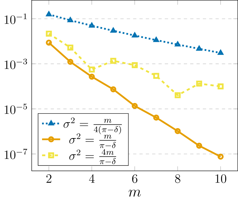
(a) $\delta=\frac{\pi}{4}$

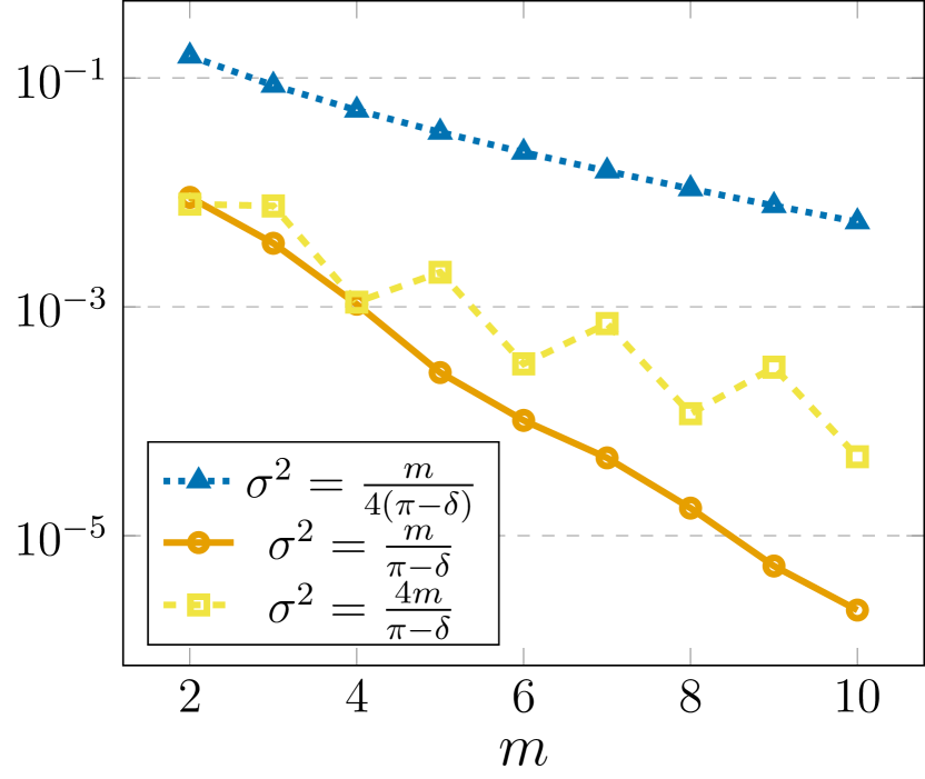
(b) $\delta=\frac{\pi}{2}$

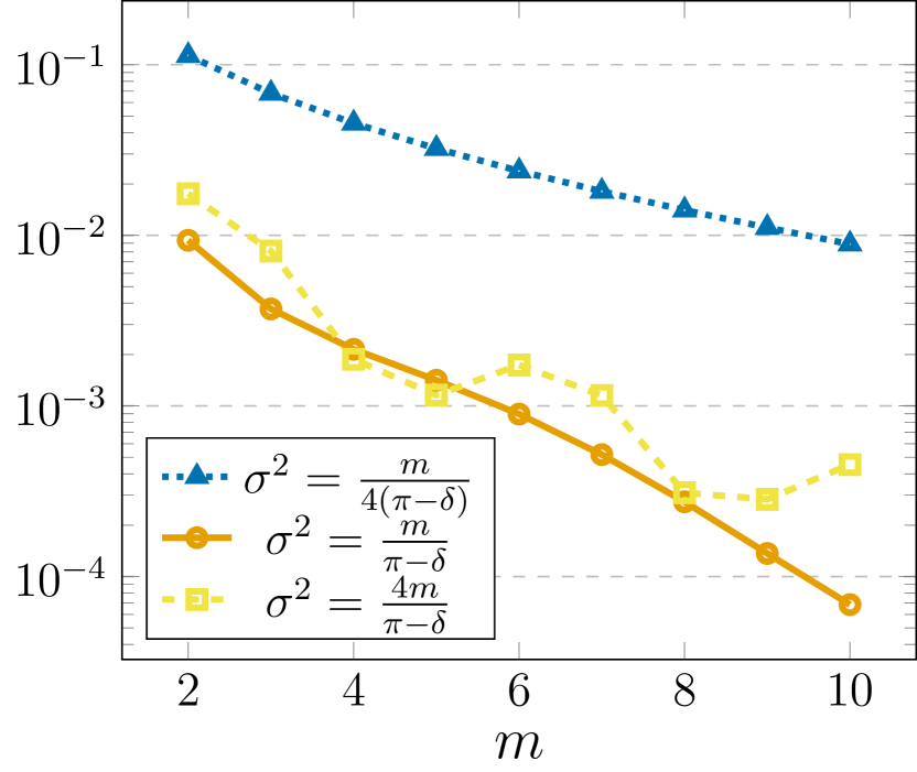
(c) $\delta=\frac{3\pi}{4}$

Figure 3.1: Maximum approximation error (3.7) using the Gaussian function $\varphi_{\mathrm{Gauss}}$ in (1.5) with different variances $\sigma^{2}\in\big{\{}\frac{m}{4(\pi-\delta)},\frac{m}{\pi-\delta},\frac{4m}{\pi-\delta}\big{\}}$, for the bandlimited function (3.8) with bandwidths $\delta\in\big{\{}\frac{\pi}{4},\frac{\pi}{2},\frac{3\pi}{4}\big{\}}$ and truncation parameters $m\in\{2,3,\ldots,10\}$.

      

Note that in [25, 24] the modified Gaussian function (1.6) was used for the regularization of Shannon sampling formulas, using a slightly different notation. By the same techniques as in Theorem 3.1 one can determine the optimal parameter $\sigma^{2}$ of (1.6) subject to $\lambda$.

Theorem 3.4.

Assume that $f\in L^{2}(\mathbb{R})\cap C(\mathbb{R})$ is bandlimited with bandwidth $\delta\in(0,\,\pi)$. Further let $\varphi_{\mathrm{modGauss}}$ be the modified Gaussian function (1.6) with parameter $\sigma^{2}=\frac{m}{\pi-\lambda-\delta}$, $0\leq\lambda<\pi-\delta$, and let $m\in{\mathbb{N}}\setminus\{1\}$ be given.
Then the modified Gaussian regularized Shannon sampling formula satisfies the error estimate

$$\big{\|}f-R_{\mathrm{modGauss},m}f\big{\|}_{C_{0}(\mathbb{R})}\leq\frac{2\sqrt{2}}{\sqrt{\pi m\,(\pi-\lambda-\delta)}}\,\mathrm{e}^{-m\,(\pi-\lambda-\delta)/2}\,\|f\|_{L^{2}(\mathbb{R})}\,.$$ (3.9)

Proof. (i) At first, we estimate the regularization error constant (2.1) for the modified Gaussian function (1.6). By [18, p. 21, 5.24] the Fourier transform of $\varphi_{\mathrm{modGauss}}$ reads as

$${\hat{\varphi}}_{\mathrm{modGauss}}(\omega) =\sigma\,\mathrm{e}^{-\sigma^{2}\,(\lambda^{2}+\omega^{2})/2}\,\cosh(\lambda\sigma^{2}\omega)=\frac{\sigma}{2}\left(\mathrm{e}^{-\sigma^{2}\,(\omega+\lambda)^{2}/2}+\mathrm{e}^{-\sigma^{2}\,(\omega-\lambda)^{2}/2}\right)\,,\quad\omega\in\mathbb{R}\,.$$

Therefore, we obtain for $\omega\in[-\delta,\,\delta]$ with $\delta\in(0,\,\pi)$ that

$$\Delta_{\mathrm{modGauss}}(\omega) \coloneqq 1-\frac{1}{\sqrt{2\pi}}\,\int_{\omega-\pi}^{\omega+\pi}{\hat{\varphi}}_{\mathrm{modGauss}}(\tau)\,\mathrm{d}\tau$$

$$=\frac{1}{2}\bigg{(}1-\frac{\sigma}{\sqrt{2\pi}}\int_{\omega-\pi}^{\omega+\pi}\mathrm{e}^{-\sigma^{2}(\tau+\lambda)^{2}/2}\,\mathrm{d}\tau\bigg{)}+\frac{1}{2}\bigg{(}1-\frac{\sigma}{\sqrt{2\pi}}\int_{\omega-\pi}^{\omega+\pi}\mathrm{e}^{-\sigma^{2}(\tau-\lambda)^{2}/2}\,\mathrm{d}\tau\bigg{)}\,.$$

Substituting $s=\sigma(\tau+\lambda)/\sqrt{2}$ in the first term and $s=\sigma(\tau-\lambda)/\sqrt{2}$ in the second term, as well as using the integral (3.2), it follows that

$$\Delta_{\mathrm{modGauss}}(\omega) =\frac{1}{2\sqrt{\pi}}\bigg{(}\int_{\mathbb{R}}\mathrm{e}^{-s^{2}}\,\mathrm{d}s-\int_{(\omega-\pi+\lambda)\sigma/\sqrt{2}}^{(\omega+\pi+\lambda)\sigma/\sqrt{2}}\mathrm{e}^{-s^{2}}\,\mathrm{d}s\bigg{)}$$

$$\qquad+\,\frac{1}{2\sqrt{\pi}}\bigg{(}\int_{\mathbb{R}}\mathrm{e}^{-s^{2}}\,\mathrm{d}s-\int_{(\omega-\pi-\lambda)\sigma/\sqrt{2}}^{(\omega+\pi-\lambda)\sigma/\sqrt{2}}\mathrm{e}^{-s^{2}}\,\mathrm{d}s\bigg{)}$$

$$=\frac{1}{2\sqrt{\pi}}\bigg{(}\int_{-\infty}^{(\omega-\pi+\lambda)\sigma/\sqrt{2}}+\int_{(\omega+\pi+\lambda)\sigma/\sqrt{2}}^{\infty}$$

$$\qquad+\,\int_{-\infty}^{(\omega-\pi-\lambda)\sigma/\sqrt{2}}+\int_{(\omega+\pi-\lambda)\sigma/\sqrt{2}}^{\infty}\bigg{)}\,\mathrm{e}^{-s^{2}}\,\mathrm{d}s$$

$$=\frac{1}{2\sqrt{\pi}}\bigg{(}\int_{(\pi-\lambda-\omega)\sigma/\sqrt{2}}^{\infty}+\int_{(\pi+\lambda+\omega)\sigma/\sqrt{2}}^{\infty}$$

$$\qquad+\,\int_{(\pi+\lambda-\omega)\sigma/\sqrt{2}}^{\infty}+\int_{(\pi-\lambda+\omega)\sigma/\sqrt{2}}^{\infty}\bigg{)}\,\mathrm{e}^{-s^{2}}\,\mathrm{d}s\,.$$

Since $\Delta_{\mathrm{modGauss}}$ is even, we consider only the case $\omega\in[0,\delta]$. By (3.3) we obtain

$$0\leq\Delta_{\mathrm{modGauss}}(\omega) \leq\frac{1}{4\sqrt{\pi}}\bigg{(}\frac{\sqrt{2}}{(\pi-\lambda-\omega)\sigma}\,\mathrm{e}^{(\pi-\lambda-\omega)^{2}\sigma^{2}/2}+\frac{\sqrt{2}}{(\pi+\lambda+\omega)\sigma}\,\mathrm{e}^{(\pi+\lambda+\omega)^{2}\sigma^{2}/2}$$

$$\qquad+\frac{\sqrt{2}}{(\pi+\lambda-\omega)\sigma}\,\mathrm{e}^{(\pi+\lambda-\omega)^{2}\sigma^{2}/2}+\frac{\sqrt{2}}{(\pi-\lambda+\omega)\sigma}\,\mathrm{e}^{(\pi-\lambda+\omega)^{2}\sigma^{2}/2}\bigg{)}$$

$$\leq\frac{1}{\sqrt{\pi}}\,\frac{\sqrt{2}}{(\pi-\lambda-\omega)\sigma}\,\mathrm{e}^{-(\pi-\lambda-\omega)^{2}\sigma^{2}/2}\,,\quad\omega\in[0,\delta]\,.$$

Consequently, we have for all $\omega\in[-\delta,\,\delta]$ that

$$0\leq\Delta_{\mathrm{modGauss}}(\omega)\leq\sqrt{\frac{2}{\pi}}\,\frac{\mathrm{e}^{-(\pi-\lambda-|\omega|)^{2}\sigma^{2}/2}}{(\pi-\lambda-|\omega|)\,\sigma}$$

and hence

$$E_{1}(m)\leq\sqrt{\frac{2}{\pi}}\,\frac{\mathrm{e}^{-(\pi-\lambda-\delta)^{2}\sigma^{2}/2}}{(\pi-\lambda-\delta)\,\sigma}\,.$$ (3.10)

(ii) For the truncation error constant (2.2) for the modified Gaussian function (1.6), we observe that by the inequalities $\varphi_{\mathrm{modGauss}}^{2}(m)\leq\mathrm{e}^{-m^{2}/\sigma^{2}}$ and

$$\int_{m}^{\infty}\varphi_{\mathrm{modGauss}}^{2}(t)\,\mathrm{d}t\leq\sigma\,\int_{m/\sigma}^{\infty}\mathrm{e}^{-s^{2}}\,\mathrm{d}s\leq\frac{\sigma^{2}}{2m}\,\mathrm{e}^{-m^{2}/\sigma^{2}}$$

we also have (3.5).
(iii) Finally, we say that the parameter $\sigma^{2}$ of the modified Gaussian function (1.6) is optimal, if $E_{1}(m)$ and $E_{2}(m)$ possess the same exponential decay with respect to $m$. From (3.10) and (3.5) it follows that

$$\sigma^{2}=\frac{m}{\pi-\lambda-\delta}$$ (3.11)

is the optimal parameter with

$$E_{1}(m) \leq\sqrt{\frac{2}{\pi}}\,\frac{1}{\sqrt{m\,(\pi-\lambda-\delta)}}\,\mathrm{e}^{-m\,(\pi-\lambda-\delta)/2}\,,$$

$$E_{2}(m) \leq\frac{\sqrt{2}}{\pi m}\,\sqrt{1+\frac{1}{2\,(\pi-\lambda-\delta)}}\,\mathrm{e}^{-m\,(\pi-\lambda-\delta)/2}\,.$$

where we have $\pi-\lambda-\delta>0$ by the assumption $\lambda\in[0,\,\pi-\delta)$.

Note that since $m\in\mathbb{N}\setminus\{1\}$, $\delta\in(0,\,\pi)$, and $\lambda\in[0,\,\pi-\delta)$, we have

$$\left(\frac{\sqrt{2}}{\sqrt{\pi m\,(\pi-\lambda-\delta)}}\right)^{-1}\cdot\frac{\sqrt{2}}{\pi m}\,\sqrt{1+\frac{1}{2\,(\pi-\lambda-\delta)}} =\sqrt{\frac{2(\pi-\lambda-\delta)+1}{2\pi m}}\leq\sqrt{\frac{2\pi+1}{4\pi}}<1$$

and therefore

$$E_{2}(m)\leq\frac{\sqrt{2}}{\sqrt{\pi m\,(\pi-\lambda-\delta)}}\,\mathrm{e}^{-m\,(\pi-\lambda-\delta)/2}\,.$$

Thus, the modified Gaussian regularized Shannon sampling formula with the optimal parameter (3.11) fulfills the error estimate (3.9). This completes the proof.  

Thereby, Theorem 3.4 shows that the approximation error of the regularized Shannon sampling formula with the modified Gaussian function (1.6) has the best exponential decay in the case $\lambda=0$. In other words, the Gaussian function $\varphi_{\mathrm{Gauss}}$ in (1.5) is much more favorable than the modified Gaussian function $\varphi_{\mathrm{modGauss}}$ in (1.6).

4 Optimal regularization with the sinh-type window function

In this section, we consider the $\sinh$-type window function (1.7) with shape parameter $\beta>0$, analogous to [12, Theorem 6.1] and [13, Theorem 4.2]. In order to achieve fast convergence of the $\sinh$-type regularized Shannon sampling formula, we put special emphasis on the optimal choice of this shape parameter $\beta$. Moreover, we demonstrate that the exponential decay with respect to the truncation parameter $m\in\mathbb{N}\setminus\{1\}$ is much better for the uniform approximation error $\big{\|}f-R_{\sinh,m}f\big{\|}_{C_{0}(\mathbb{R})}$ than for the approximation error $\big{\|}f-R_{\mathrm{Gauss},m}f\big{\|}_{C_{0}(\mathbb{R})}$ in Theorem 3.1.

Theorem 4.1.

Assume that $f\in L^{2}(\mathbb{R})\cap C(\mathbb{R})$ is bandlimited with bandwidth $\delta\in(0,\,\pi)$. Further let $\varphi_{\sinh}$ be the $\sinh$-type window function (1.7) with shape parameter $\beta=m\,(\pi-\delta)$ and let $m\in{\mathbb{N}}\setminus\{1\}$ be given.
Then the $\sinh$-type regularized Shannon sampling formula satisfies the error estimate

$$\big{\|}f-R_{\sinh,m}f\big{\|}_{C_{0}(\mathbb{R})}\leq\mathrm{e}^{-m\,(\pi-\delta)}\,\|f\|_{L^{2}(\mathbb{R})}\,.$$ (4.1)

Proof. (i) Since $\varphi_{\sinh}$ in (1.7) is compactly supported on $[-m,\,m]$ and $\varphi_{\sinh}(m)=0$, we have $E_{2}(m)=0$. Thus, according to Theorem 2.1, the approximation error can be estimated by

$$\big{\|}f-R_{\sinh,m}f\big{\|}_{C_{0}(\mathbb{R})}\leq\|f\|_{L^{2}(\mathbb{R})}\,\max_{\omega\in[-\delta,\delta]}\big{|}\Delta_{\sinh}(\omega)\big{|}\,,$$

where

$$\Delta_{\sinh}(\omega)\coloneqq 1-\frac{1}{\sqrt{2\pi}}\,\int_{\omega-\pi}^{\omega+\pi}{\hat{\varphi}}_{\sinh}(\tau)\,\mathrm{d}\tau\,,\quad\omega\in[-\delta,\,\delta]\,.$$ (4.2)

Following [18, p. 38, 7.58], the Fourier transform of (1.7) has the form

$${\hat{\varphi}}_{\sinh}(\tau)=\frac{m\,\sqrt{\pi}}{\sqrt{2}\,\sinh\beta}\cdot\begin{cases}(1-\nu^{2})^{-1/2}\,I_{1}\big{(}\beta\,\sqrt{1-\nu^{2}}\big{)}&\colon|\nu|<1\,,\\[4.30554pt] (\nu^{2}-1)^{-1/2}\,J_{1}\big{(}\beta\,\sqrt{\nu^{2}-1}\big{)}&\colon|\nu|>1\,,\end{cases}$$ (4.3)

with the scaled frequency $\nu=\frac{m}{\beta}\,\tau$, where $J_{1}$ denotes the Bessel function and $I_{1}$ the modified Bessel function of first order. Substituting $\tau=\frac{\beta}{m}\,\nu$ in the integral in (4.2), the function $\Delta_{\sinh}$ reads as

$$\Delta_{\sinh}(\omega)\coloneqq 1-\frac{\beta}{\sqrt{2\pi}\,m}\,\int_{-\nu_{1}(-\omega)}^{\nu_{1}(\omega)}{\hat{\varphi}}_{\sinh}\big{(}\tfrac{\beta}{m}\,\nu\big{)}\,\mathrm{d}\nu\,,\quad\omega\in[-\delta,\,\delta]\,,$$ (4.4)

with the increasing linear function

$$\nu_{1}(\omega)\coloneqq\frac{m}{\beta}\,(\omega+\pi)\,,\quad\omega\in[-\delta,\,\delta]\,.$$ (4.5)

(ii) Now we choose the shape parameter of (1.7) in the special form $\beta=m\,(\pi-\delta)$. Thus, we have

$$1=\nu_{1}(-\delta)\leq\nu_{1}(\omega)=\frac{\omega+\pi}{\pi-\delta}\leq\nu_{1}(\delta)=\frac{\pi+\delta}{\pi-\delta}\,,\quad\omega\in[-\delta,\,\delta]\,.$$

In view of (4.3) we split (4.4) in the form $\Delta_{\sinh}(\omega)=\Delta_{\sinh,1}-\Delta_{\sinh,2}(\omega)$ with

$$\Delta_{\sinh,1} \coloneqq 1-\frac{\beta}{\sinh\beta}\,\int_{0}^{1}\frac{I_{1}\big{(}\beta\,\sqrt{1-\nu^{2}}\big{)}}{\sqrt{1-\nu^{2}}}\,\mathrm{d}\nu\,,$$

$$\Delta_{\sinh,2}(\omega) \coloneqq\frac{\beta}{2\,\sinh\beta}\,\bigg{(}\int_{1}^{\nu_{1}(-\omega)}+\int_{1}^{\nu_{1}(\omega)}\bigg{)}\,\frac{J_{1}\big{(}\beta\,\sqrt{\nu^{2}-1}\big{)}}{\sqrt{\nu^{2}-1}}\,\mathrm{d}\nu\,.$$

Using [10, 6.681–11] and [1, 10.2.13], we get

$$\int_{0}^{1}\frac{I_{1}\big{(}\beta\,\sqrt{1-\nu^{2}}\big{)}}{\sqrt{1-\nu^{2}}}\,\mathrm{d}\nu=\int_{0}^{\pi/2}I_{1}(\beta\,\cos\sigma)\,\mathrm{d}\sigma=\frac{\pi}{2}\,\bigg{(}I_{1/2}\bigg{(}\frac{\beta}{2}\bigg{)}\bigg{)}^{2}=\frac{2}{\beta}\left(\sinh\frac{\beta}{2}\right)^{2}$$ (4.6)

and hence

$$\Delta_{\sinh,1}=1-\frac{2\,\big{(}\sinh\frac{\beta}{2}\big{)}^{2}}{\sinh\beta}=\frac{2\,\mathrm{e}^{-\beta}}{1+\mathrm{e}^{-\beta}}\,.$$ (4.7)

By [10, 6.645–1] we have

$$\int_{1}^{\infty}\frac{J_{1}\big{(}\beta\,\sqrt{\nu^{2}-1}\big{)}}{\sqrt{\nu^{2}-1}}\,\mathrm{d}\nu=I_{1/2}\bigg{(}\frac{\beta}{2}\bigg{)}\,K_{1/2}\bigg{(}\frac{\beta}{2}\bigg{)}=\frac{1-\mathrm{e}^{-\beta}}{\mathrm{e}^{\beta}}\,,$$

where $I_{1/2}$ and $K_{1/2}$ are modified Bessel functions of half order (see [1, 10.2.13, 10.2.14, and 10.2.17]. Numerical experiments, cf. [12], have shown that for all $W>1$ we have

$$0<\int_{1}^{W}\frac{J_{1}\big{(}\beta\,\sqrt{\nu^{2}-1}\big{)}}{\sqrt{\nu^{2}-1}}\,\mathrm{d}\nu\leq\frac{3\,(1-\mathrm{e}^{-\beta})}{2\,\beta}\,,$$ (4.8)

such that

$$0\leq\Delta_{\sinh,2}(\omega)\leq\frac{\beta}{2\,\sinh\beta}\,\frac{3\,(1-\mathrm{e}^{-\beta})}{\beta}=\frac{3\,\mathrm{e}^{-\beta}}{1+\mathrm{e}^{-\beta}}\,,\quad\omega\in[-\delta,\,\delta]\,.$$ (4.9)

Thereby, it follows from (4.7) and (4.9) that the expressions in (4.12) have the same exponential decay $m\,(\pi-\delta)$ and that

$$\big{|}\Delta_{\sinh}(\omega)\big{|}=\big{|}\Delta_{\sinh,1}-\Delta_{\sinh,2}(\omega)\big{|}\leq\frac{\mathrm{e}^{-\beta}}{1+\mathrm{e}^{-\beta}}<\mathrm{e}^{-\beta}\,,\quad\omega\in[-\delta,\,\delta]\,.$$

Thus, the $\sinh$-type regularized Shannon sampling formula with the chosen shape parameter $\beta=m\,(\pi-\delta)$ fulfills the error estimate (4.1). This completes the proof.  

Now we show that the choice of the shape parameter $\beta=m\,(\pi-\delta)$ of (1.7) is optimal in a certain sense. To this end, let the parameters $\alpha>0$, $m\in\mathbb{N}\setminus\{1\}$, and $\delta\in(0,\pi)$ be given, and consider shape parameters of the form $\beta=\alpha\,m\,(\pi-\delta)$. Then the increasing linear function (4.5) fulfills

$$\frac{1}{\alpha}=\nu_{1}(-\delta)\leq\nu_{1}(\omega)=\frac{\omega+\pi}{\alpha\,(\pi-\delta)}\leq\nu_{1}(\delta)=\frac{\pi+\delta}{\alpha\,(\pi-\delta)}\,,\quad\omega\in[-\delta,\,\delta]\,.$$

Therefore, we split (4.4) as $\Delta_{\sinh}(\omega)=\Delta_{\sinh,1}-\Delta_{\sinh,2}(\omega)$, $\omega\in[-\delta,\,\delta]$, with

$$\Delta_{\sinh,1} \coloneqq 1-\frac{\beta}{m\,\sqrt{2\pi}}\,\int_{-1/\alpha}^{1/\alpha}{\hat{\varphi}}_{\sinh}\big{(}\tfrac{\beta}{m}\,\nu\big{)}\,\mathrm{d}\nu$$

$$=1-\frac{\beta\,\sqrt{2}}{m\,\sqrt{\pi}}\,\int_{0}^{1/\alpha}{\hat{\varphi}}_{\sinh}\big{(}\tfrac{\beta}{m}\,\nu\big{)}\,\mathrm{d}\nu\,,$$ (4.10)

and

$$\Delta_{\sinh,2}(\omega) \coloneqq\frac{\beta}{m\,\sqrt{2\pi}}\,\bigg{(}\int_{-\nu_{1}(-\omega)}^{-1/\alpha}+\int_{1/\alpha}^{\nu_{1}(\omega)}\bigg{)}\,{\hat{\varphi}}_{\sinh}\big{(}\tfrac{\beta}{m}\,\nu\big{)}\,\mathrm{d}\nu$$

$$=\frac{\beta}{m\,\sqrt{2\pi}}\,\bigg{(}\int_{1/\alpha}^{\nu_{1}(-\omega)}+\int_{1/\alpha}^{\nu_{1}(\omega)}\bigg{)}\,{\hat{\varphi}}_{\sinh}\big{(}\tfrac{\beta}{m}\,\nu\big{)}\,\mathrm{d}\nu\,.$$ (4.11)

Introducing the terms

$$D_{1}(m)\coloneqq\big{|}\Delta_{\sinh,1}\big{|}\,,\quad D_{2}(m)\coloneqq\max_{\omega\in[-\delta,\delta]}\big{|}\Delta_{\sinh,2}(\omega)\big{|}\,,$$ (4.12)

it is known by Theorem 4.1 that for $\alpha=1$ both expressions in (4.12) possess the same exponential decay $m\,(\pi-\delta)$. In the following, we discuss the other cases $0<\alpha<1$ and $\alpha>1$. More precisely, we show in Theorem 4.2 that for $\alpha\neq 1$ both expressions in (4.12) have the same exponential decay smaller than $m\,(\pi-\delta)$. In this sense, it follows immediately that the shape parameter $\beta=m\,(\pi-\delta)$ of the $\sinh$-type window function (1.7) is optimal, since both expressions in (4.12) tend to zero as $m\to\infty$ with the same maximum exponential decay.

Theorem 4.2.

For $\delta\in(0,\,\pi)$, let $\varphi_{\sinh}$ be the $\sinh$-type window function (1.7) with the shape parameter $\beta=\alpha\,m\,(\pi-\delta)$ with $\alpha>0$, $\alpha\not=1$, and $m\in{\mathbb{N}}\setminus\{1\}$.

1. In the case $\alpha\in(0,\,1)$, both expressions in (4.12) tend to zero as $m\to\infty$ with the same exponential decay $\alpha\,m\,(\pi-\delta)$.

2. In the case $\alpha>1$, both expressions in (4.12) tend to zero as $m\to\infty$ with exponential decay smaller than $m\,(\pi-\delta)$.

Proof. a) First we consider the shape parameter $\beta=\alpha\,m\,(\pi-\delta)$ with $\alpha\in(0,\,1)$. Then we have by (4.10), (4.3) and (4.6) that

$$\Delta_{\sinh,1} =1-\frac{\beta\,\sqrt{2}}{m\,\sqrt{\pi}}\,\int_{0}^{1/\alpha}{\hat{\varphi}}_{\sinh}\big{(}\tfrac{\beta}{m}\,\nu\big{)}\,{\mathrm{d}}\nu$$

$$=1-\frac{\beta\,\sqrt{2}}{m\,\sqrt{\pi}}\,\bigg{(}\int_{0}^{1}+\int_{1}^{1/\alpha}\bigg{)}\,{\hat{\varphi}}_{\sinh}\big{(}\tfrac{\beta}{m}\,\nu\big{)}\,{\mathrm{d}}\nu$$

$$=\bigg{(}1-\frac{\beta}{\sinh\beta}\,\int_{0}^{1}\frac{I_{1}\big{(}\beta\,\sqrt{1-\nu^{2}}\big{)}}{\sqrt{1-\nu^{2}}}\,{\mathrm{d}}\nu\bigg{)}-\frac{\beta}{\sinh\beta}\,\int_{1}^{1/\alpha}\frac{J_{1}\big{(}\beta\,\sqrt{\nu^{2}-1}\big{)}}{\sqrt{\nu^{2}-1}}\,{\mathrm{d}}\nu$$

$$=\bigg{(}1-\frac{2\,\big{(}\sinh\frac{\beta}{2}\big{)}^{2}}{\sinh\beta}\bigg{)}-\frac{\beta}{\sinh\beta}\,\int_{1}^{1/\alpha}\frac{J_{1}\big{(}\beta\,\sqrt{\nu^{2}-1}\big{)}}{\sqrt{\nu^{2}-1}}\,{\mathrm{d}}\nu$$

$$=\frac{2\,\mathrm{e}^{-\beta}}{1+\mathrm{e}^{-\beta}}-\frac{\beta}{\sinh\beta}\,\int_{1}^{1/\alpha}\frac{J_{1}\big{(}\beta\,\sqrt{\nu^{2}-1}\big{)}}{\sqrt{\nu^{2}-1}}\,{\mathrm{d}}\nu\,.$$

Hence, by (4.8) this yields

$$\big{|}\Delta_{\sinh,1}\big{|}\leq\frac{2\,\mathrm{e}^{-\beta}}{1+\mathrm{e}^{-\beta}}+\frac{\beta}{\sinh\beta}\,\frac{3\,(1-\mathrm{e}^{-\beta})}{2\,\beta}=\frac{5\,\mathrm{e}^{-\beta}}{1+\mathrm{e}^{-\beta}}\,.$$ (4.13)

For the second term (4.11) we have by (4.3) that

$$\Delta_{\sinh,2}(\omega) =\frac{\beta}{m\,\sqrt{2\,\pi}}\,\bigg{(}\int_{1/\alpha}^{\nu_{1}(-\omega)}+\int_{1/\alpha}^{\nu_{1}(\omega)}\bigg{)}{\hat{\varphi}}_{\sinh}\big{(}\tfrac{\beta}{m}\,\nu\big{)}\,{\mathrm{d}}\nu$$

$$=\frac{\beta}{2\,\sinh\beta}\,\bigg{(}\int_{1/\alpha}^{\nu_{1}(-\omega)}+\int_{1/\alpha}^{\nu_{1}(\omega)}\bigg{)}\frac{J_{1}\big{(}\beta\,\sqrt{\nu^{2}-1}\big{)}}{\sqrt{\nu^{2}-1}}\,{\mathrm{d}}\nu$$

$$=\frac{\beta}{2\,\sinh\beta}\,\bigg{(}\int_{1}^{\nu_{1}(-\omega)}+\int_{1}^{\nu_{1}(\omega)}-2\,\int_{1}^{1/\alpha}\bigg{)}\frac{J_{1}\big{(}\beta\,\sqrt{\nu^{2}-1}\big{)}}{\sqrt{\nu^{2}-1}}\,{\mathrm{d}}\nu\,,\quad\omega\in[-\delta,\,\delta]\,,$$

such that (4.8) implies

$$\big{|}\Delta_{\sinh,2}(\omega)\big{|}\leq\frac{3\,\big{(}1-\mathrm{e}^{-\beta}\big{)}}{\sinh\beta}=\frac{6\,\mathrm{e}^{-\beta}}{1+\mathrm{e}^{-\beta}}\,,\quad\omega\in[-\delta,\,\delta]\,.$$ (4.14)

Thus, by (4.13) and (4.14) the quantities (4.12) tend to zero as $m\to\infty$ with the same exponential decay $\alpha\,m\,(\pi-\delta)$, which is smaller than $m\,(\pi-\delta)$ as $\alpha\in(0,\,1)$.

b) Now we investigate the shape parameter $\beta=\alpha\,m\,(\pi-\delta)$ with $\alpha>1$.
(i) By (4.10) and (4.3) we obtain

$$\Delta_{\sinh,1} =1-\frac{\beta\,\sqrt{2}}{m\,\sqrt{\pi}}\,\int_{0}^{1/\alpha}{\hat{\varphi}}_{\sinh}\big{(}\tfrac{\beta}{m}\,\nu\big{)}\,{\mathrm{d}}\nu=1-\frac{\beta}{\sinh\beta}\,\int_{0}^{1/\alpha}\frac{I_{1}\big{(}\beta\,\sqrt{1-\nu^{2}}\big{)}}{\sqrt{1-\nu^{2}}}\,\mathrm{d}\nu\,.$$

Numerical experiments, cf. Figure 4.1, have shown that

$$\Delta_{\sinh,1}>1-\frac{m\,(\pi-\delta)}{\sinh\big{(}m\,(\pi-\delta)\big{)}}\,\int_{0}^{1}\frac{I_{1}\big{(}m\,(\pi-\delta)\,\sqrt{1-\nu^{2}}\big{)}}{\sqrt{1-\nu^{2}}}\,\mathrm{d}\nu\,.$$

Hence, by (4.6) we have

$$\Delta_{\sinh,1}>1-\frac{2\,\big{(}\sinh\big{(}\frac{m\,(\pi-\delta)}{2}\big{)}\big{)}^{2}}{\sinh\big{(}m\,(\pi-\delta)\big{)}}=\frac{2\,\mathrm{e}^{-m\,(\pi-\delta)}}{1+\mathrm{e}^{-m\,(\pi-\delta)}}>0\,,$$

i. e., $D_{1}(m)=\Delta_{\sinh,1}$ tends to zero as $m\to\infty$ with exponential decay smaller than $m\,(\pi-\delta)$.

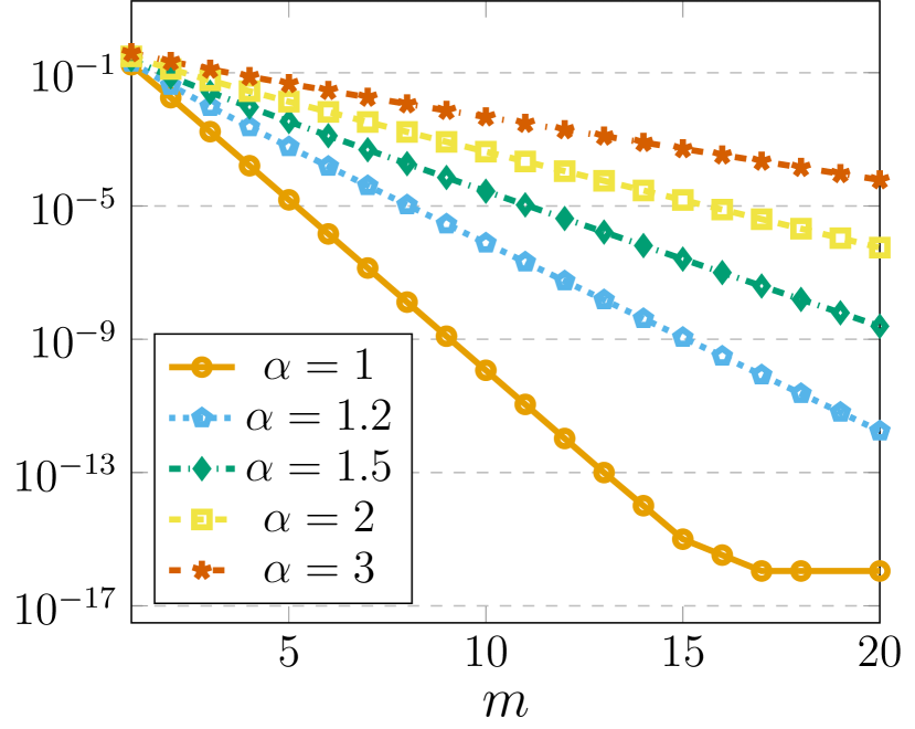
(a) $\delta=\frac{\pi}{4}$

(b) $\delta=\frac{\pi}{2}$

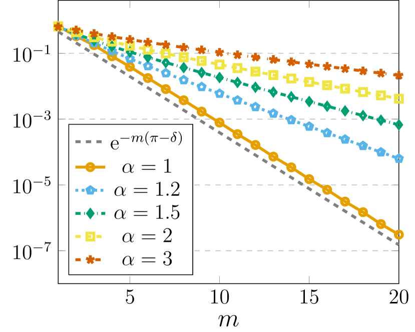
(c) $\delta=\frac{3\pi}{4}$

Figure 4.1: Semilogarithmic plots of the term $1-\frac{\beta}{\sinh\beta}\,\int_{0}^{1/\alpha}\frac{I_{1}(\beta\sqrt{1-\nu^{2}})}{\sqrt{1-\nu^{2}}}\,\mathrm{d}\nu$ for $m=1,\ldots,20$, $\alpha\in\{1,\,1.2,\,1.5,\,2,\,3\}$, and $\delta\in\big{\{}\frac{\pi}{4},\,\frac{\pi}{2},\,\frac{3\pi}{4}\big{\}}$.

(ii) On the one hand, we consider the expression (4.11) in the case

$$1<\frac{\pi+\delta}{\pi-\delta}\leq\alpha\,,$$

i. e., for (4.5) we have $\nu_{1}(\delta)=\frac{\pi+\delta}{\alpha\,(\pi-\delta)}\leq 1$, such that

$$\frac{1}{\alpha}\leq\nu_{1}(\pm\omega)\leq 1\,,\quad\omega\in[-\delta,\,\delta]\,.$$ (4.15)

Then by (4.11) and (4.3) we obtain

$$0<\Delta_{\sinh,2}(\omega) =\frac{\beta}{2\,\sinh\beta}\,\bigg{(}\int_{1/\alpha}^{\nu_{1}(-\omega)}+\int_{1/\alpha}^{\nu_{1}(\omega)}\bigg{)}\frac{I_{1}\big{(}\beta\,\sqrt{1-\nu^{2}}\big{)}}{\sqrt{1-\nu^{2}}}\,\mathrm{d}\nu\,,\quad\omega\in[-\delta,\,\delta]\,.$$

Note that by (4.5) and (4.15) we have $\frac{1}{\alpha}<\nu_{1}(0)=\frac{\pi}{\alpha\,(\pi-\delta)}<1$, and

$$\nu_{1}(\omega)=\nu_{1}(0)+\frac{\omega}{\alpha\,(\pi-\delta)}\,,\quad\nu_{1}(-\omega)=\nu_{1}(0)-\frac{\omega}{\alpha\,(\pi-\delta)}\,.$$ (4.16)

Hence, for $\omega\in[0\,,\delta]$ it follows that

$$\Delta_{\sinh,2}(\omega) =\frac{\beta}{\sinh\beta}\,\int_{1/\alpha}^{\nu_{1}(0)}\frac{I_{1}\big{(}\beta\,\sqrt{1-\nu^{2}}\big{)}}{\sqrt{1-\nu^{2}}}\,\mathrm{d}\nu$$

$$\qquad+\frac{\beta}{2\,\sinh\beta}\,\Bigg{(}\int_{\nu_{1}(0)}^{\nu_{1}(0)+\frac{\omega}{\alpha(\pi-\delta)}}-\int_{\nu_{1}(0)-\frac{\omega}{\alpha(\pi-\delta)}}^{\nu_{1}(0)}\Bigg{)}\frac{I_{1}\big{(}\beta\,\sqrt{1-\nu^{2}}\big{)}}{\sqrt{1-\nu^{2}}}\,\mathrm{d}\nu\,.$$ (4.17)

An analogous decomposition of $\Delta_{\sinh,2}(\omega)$ also applies for $\omega\in[-\delta\,,0]$. By the power series expansion of the modified Bessel function $I_{1}$, the integrand

$$\frac{I_{1}(\beta\,\sqrt{1-\nu^{2}})}{\sqrt{1-\nu^{2}}}=\frac{\beta}{2}\,\sum_{k=0}^{\infty}\frac{(1-\nu^{2})^{k}}{2^{2k}k!(k+1)!}\,,\quad\nu\in(-1,\,1)\,,$$ (4.18)

is positive for $\nu\in(-1,1)$. Since the integrand $\frac{I_{1}(\beta\sqrt{1-\nu^{2}})}{\sqrt{1-\nu^{2}}}$ is also monotonously decreasing on $[0,1)$, the second term in (4) is negative for $\omega\in(0\,,\delta]$ as we have two integration intervals of the same length by (4.16), and therefore

$$D_{2}(m)=\max_{\omega\in[-\delta,\delta]}\Delta_{\sinh,2}(\omega)=\frac{\beta}{\sinh\beta}\,\int_{1/\alpha}^{\nu_{1}(0)}\frac{I_{1}(\beta\,\sqrt{1-\nu^{2}})}{\sqrt{1-\nu^{2}}}\,\mathrm{d}\nu\,.$$ (4.19)

Numerical experiments, cf. Figure 4.2, have shown that (4.19), tends to zero as $m\to\infty$ with exponential decay smaller than $m\,(\pi-\delta)$.

(a) $\delta=\frac{\pi}{4}$

(b) $\delta=\frac{\pi}{2}$

(c) $\delta=\frac{3\pi}{4}$

Figure 4.2: Semilogarithmic plots of the term $\frac{\beta}{\sinh\beta}\,\int_{1/\alpha}^{v_{1}(0)}\frac{I_{1}(\beta\sqrt{1-\nu^{2}})}{\sqrt{1-\nu^{2}}}\,\mathrm{d}\nu$ for $m=1,\ldots,20$, $\alpha\in\{1.1,\,1.2,\,1.5,\,2,\,3\}$, and $\delta\in\big{\{}\frac{\pi}{4},\,\frac{\pi}{2},\,\frac{3\pi}{4}\big{\}}$.

(iii) On the other hand, we consider the expression (4.11) in the case

$$1<\alpha<\frac{\pi+\delta}{\pi-\delta}\,.$$

Then by (4.5) we have $\nu_{1}(\omega_{1})=1$ for $\omega_{1}\coloneqq\alpha\,(\pi-\delta)-\pi$. Without loss of generality, we can assume that $\omega_{1}\geq 0$. In the case $\omega_{1}>0$, we split the interval $[-\delta,\delta]$ into the three subintervals $[-\delta,-\omega_{1}]$, $[-\omega_{1},\omega_{1}]$, and $[\omega_{1},\delta]$. In the case $\omega_{1}=0$, the interval $[-\delta,\delta]$ is decomposed into $[-\delta,0]$ and $[0,\delta]$. In the following, we discuss only the case $\omega_{1}>0$.

(A) Since $\nu_{1}(\omega)$ in (4.5) is an increasing linear function, we have for $\omega\in[-\delta,-\omega_{1}]$ that

$$\frac{1}{\alpha}\leq\nu_{1}(\omega)\leq\nu_{1}(-\omega_{1})<1\,,\quad 1\leq\nu_{1}(-\omega)\leq\nu_{1}(\delta)=\frac{\pi+\delta}{\alpha\,(\pi-\delta)}\,.$$ (4.20)

Then from (4.11) and (4.3) it follows that

$$\Delta_{\sinh,2}(\omega) =\frac{\beta}{m\,\sqrt{2\pi}}\,\bigg{(}\int_{1/\alpha}^{1}+\int_{1}^{\nu_{1}(-\omega)}+\int_{1/\alpha}^{\nu_{1}(\omega)}\bigg{)}\,{\hat{\varphi}}_{\sinh}\big{(}\tfrac{\beta}{m}\,\nu\big{)}\,{\mathrm{d}}\nu$$

$$=\frac{\beta}{2\,\sinh\beta}\,\bigg{(}\int_{1/\alpha}^{1}+\int_{1/\alpha}^{\nu_{1}(\omega)}\bigg{)}\frac{I_{1}\big{(}\beta\,\sqrt{1-\nu^{2}}\big{)}}{\sqrt{1-\nu^{2}}}\,\mathrm{d}\nu$$

$$\qquad+\,\frac{\beta}{2\,\sinh\beta}\,\int_{1}^{\nu_{1}(-\omega)}\frac{J_{1}\big{(}\beta\,\sqrt{\nu^{2}-1}\big{)}}{\sqrt{\nu^{2}-1}}\,\mathrm{d}\nu\,,\quad\omega\in[-\delta,-\omega_{1}]\,.$$

Since the integrand $\frac{I_{1}(\beta\sqrt{1-\nu^{2}})}{\sqrt{1-\nu^{2}}}$ is nonnegative by (4.18), using (4.20) and (4.8) implies

$$\frac{\beta}{2\,\sinh\beta}\,\int_{1/\alpha}^{1}\frac{I_{1}\big{(}\beta\,\sqrt{1-\nu^{2}}\big{)}}{\sqrt{1-\nu^{2}}}\,\mathrm{d}\nu <\Delta_{\sinh,2}(\omega)$$

$$<\frac{\beta}{\sinh\beta}\,\int_{1/\alpha}^{1}\frac{I_{1}\big{(}\beta\,\sqrt{1-\nu^{2}}\big{)}}{\sqrt{1-\nu^{2}}}\,\mathrm{d}\nu+\frac{\beta}{2\,\sinh\beta}\,\frac{3\,\big{(}1-\mathrm{e}^{-\beta}\big{)}}{2\,\beta}$$

$$=\frac{\beta}{\sinh\beta}\,\int_{1/\alpha}^{1}\frac{I_{1}\big{(}\beta\,\sqrt{1-\nu^{2}}\big{)}}{\sqrt{1-\nu^{2}}}\,\mathrm{d}\nu+\frac{3\,\mathrm{e}^{-\beta}}{2\,(1+\mathrm{e}^{-\beta})}\,.$$

Numerical experiments, cf. Figure 4.3, have shown that

$$\frac{\beta}{\sinh\beta}\,\int_{1/\alpha}^{1}\frac{I_{1}\big{(}\beta\,\sqrt{1-\nu^{2}}\big{)}}{\sqrt{1-\nu^{2}}}\,\mathrm{d}\nu\,,\quad\alpha>1\,,$$

tends to zero as $m\to\infty$ with exponential decay smaller than $m\,(\pi-\delta)$. Therefore, we obtain that

$$\max_{\omega\in[-\delta,-\omega_{1}]}\Delta_{\sinh,2}(\omega)$$

tends to zero as $m\to\infty$ with exponential decay smaller than $m\,(\pi-\delta)$.

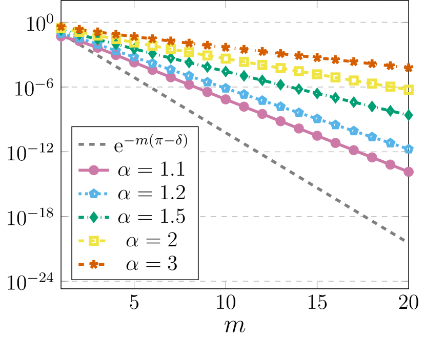
(a) $\delta=\frac{\pi}{4}$

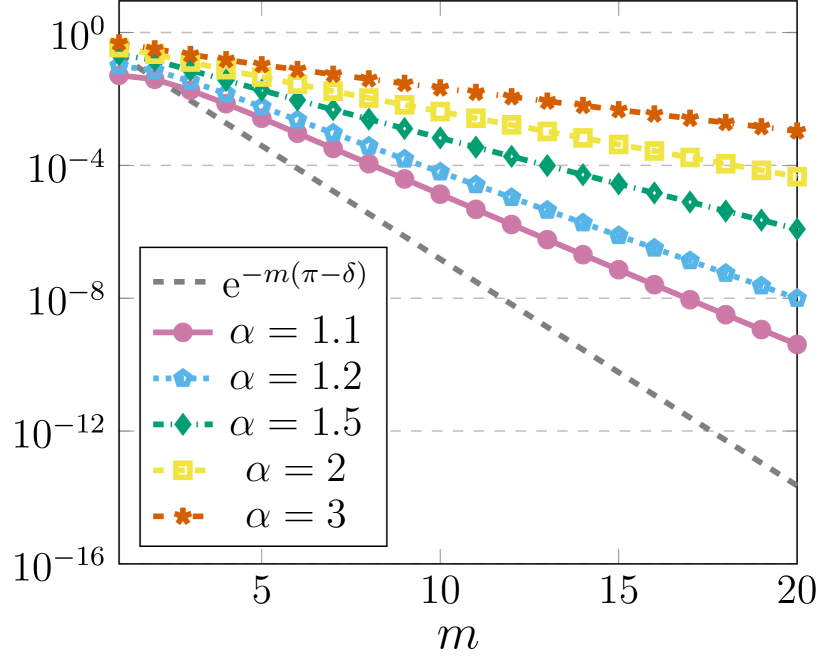
(b) $\delta=\frac{\pi}{2}$

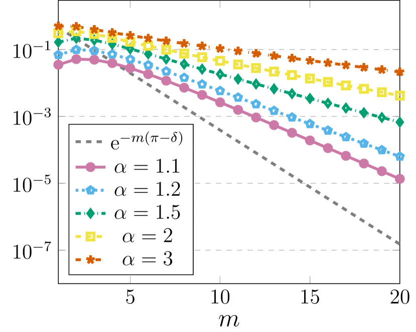
(c) $\delta=\frac{3\pi}{4}$

Figure 4.3: Semilogarithmic plots of the term $\frac{\beta}{\sinh\beta}\,\int_{1/\alpha}^{1}\frac{I_{1}(\beta\sqrt{1-\nu^{2}})}{\sqrt{1-\nu^{2}}}\,\mathrm{d}\nu$ for $m=1,\ldots,20$, $\alpha\in\{1.1,\,1.2,\,1.5,\,2,\,3\}$, and $\delta\in\big{\{}\frac{\pi}{4},\,\frac{\pi}{2},\,\frac{3\pi}{4}\big{\}}$.

(B) For $\omega\in[-\omega_{1},\omega_{1}]$ we have

$$\frac{1}{\alpha}<\nu_{1}(-\omega_{1})\leq\nu_{1}(\pm\omega)\leq 1\,.$$ (4.21)

Then from (4.11) and (4.3) it follows that

$$\Delta_{\sinh,2}(\omega) =\frac{\beta}{m\,\sqrt{2\pi}}\,\bigg{(}\int_{1/\alpha}^{\nu_{1}(-\omega)}+\int_{1/\alpha}^{\nu_{1}(\omega)}\bigg{)}\,{\hat{\varphi}}_{\sinh}\big{(}\tfrac{\beta}{m}\,\nu\big{)}\,{\mathrm{d}}\nu$$

$$=\frac{\beta}{2\,\sinh\beta}\,\bigg{(}\int_{1/\alpha}^{\nu_{1}(-\omega)}+\int_{1/\alpha}^{\nu_{1}(\omega)}\bigg{)}\frac{I_{1}\big{(}\beta\,\sqrt{1-\nu^{2}}\big{)}}{\sqrt{1-\nu^{2}}}\,\mathrm{d}\nu\,,\quad\omega\in[-\omega_{1},\omega_{1}]\,.$$

Note that by (4.5) and (4.21) we have again (4.16) and therefore (4) holds for $\omega\in[0\,,\omega_{1}]$. Analogous to (4.19) this implies

$$\max_{\omega\in[-\omega_{1},\omega_{1}]}\Delta_{\sinh,2}(\omega)=\frac{\beta}{\sinh\beta}\int_{1/\alpha}^{\nu_{1}(0)}\frac{I_{1}(\beta\sqrt{1-\nu^{2}})}{\sqrt{1-\nu^{2}}}\mathrm{d}\nu\,.$$

Hence, by the numerical experiments in Figure 4.2 we see that

$$\max_{\omega\in[-\omega_{1},\omega_{1}]}\Delta_{\sinh,2}(\omega)$$

tends to zero as $m\to\infty$ with exponential decay smaller than $m\,(\pi-\delta)$.

(C) For $\omega\in[\omega_{1},\delta]$ we have

$$1\leq\nu_{1}(\omega)\leq\nu_{1}(\delta)=\frac{\pi+\delta}{\alpha\,(\pi-\delta)}\,,\quad\frac{1}{\alpha}\leq\nu_{1}(-\omega)\leq\nu_{1}(-\omega_{1})<1\,.$$ (4.22)

Then from (4.11) and (4.3) it follows that

$$\Delta_{\sinh,2}(\omega) =\frac{\beta}{m\,\sqrt{2\pi}}\,\bigg{(}\int_{1/\alpha}^{\nu_{1}(-\omega)}+\int_{1/\alpha}^{1}+\int_{1}^{\nu_{1}(\omega)}\bigg{)}\,{\hat{\varphi}}_{\sinh}\big{(}\tfrac{\beta}{m}\,\nu\big{)}\,{\mathrm{d}}\nu$$

$$=\frac{\beta}{2\,\sinh\beta}\,\bigg{(}\int_{1/\alpha}^{\nu_{1}(-\omega)}+\int_{1/\alpha}^{1}\bigg{)}\frac{I_{1}\big{(}\beta\,\sqrt{1-\nu^{2}}\big{)}}{\sqrt{1-\nu^{2}}}\,\mathrm{d}\nu$$

$$\qquad+\,\frac{\beta}{2\,\sinh\beta}\,\int_{1}^{\nu_{1}(\omega)}\frac{J_{1}\big{(}\beta\,\sqrt{\nu^{2}-1}\big{)}}{\sqrt{\nu^{2}-1}}\,\mathrm{d}\nu\,.$$

Since the integrand $\frac{I_{1}(\beta\sqrt{1-\nu^{2}})}{\sqrt{1-\nu^{2}}}$ is nonnegative by (4.18), using (4.22) and (4.8) implies

$$\frac{\beta}{2\,\sinh\beta}\,\int_{1/\alpha}^{1}\frac{I_{1}\big{(}\beta\,\sqrt{1-\nu^{2}}\big{)}}{\sqrt{1-\nu^{2}}}\,\mathrm{d}\nu <\Delta_{\sinh,2}(\omega)$$

$$<\frac{\beta}{\sinh\beta}\,\int_{1/\alpha}^{1}\frac{I_{1}\big{(}\beta\,\sqrt{1-\nu^{2}}\big{)}}{\sqrt{1-\nu^{2}}}\,\mathrm{d}\nu+\frac{\beta}{2\,\sinh\beta}\,\frac{3\,\big{(}1-\mathrm{e}^{-\beta}\big{)}}{2\,\beta}$$

$$=\frac{\beta}{\sinh\beta}\,\int_{1/\alpha}^{1}\frac{I_{1}\big{(}\beta\,\sqrt{1-\nu^{2}}\big{)}}{\sqrt{1-\nu^{2}}}\,\mathrm{d}\nu+\frac{3\,\mathrm{e}^{-\beta}}{2\,(1+\mathrm{e}^{-\beta})}\,.$$

Hence, by the numerical experiments in Figure 4.3 we obtain that

$$\max_{\omega\in[\omega_{1},\delta]}\Delta_{\sinh,2}(\omega)$$

tends to zero as $m\to\infty$ with exponential decay smaller than $m\,(\pi-\delta)$.

In summary,

$$D_{2}(m)=\max_{\omega\in[-\delta,\delta]}\Delta_{\sinh,2}(\omega)$$

tends to zero for $m\to\infty$ with exponential decay smaller than $m\,(\pi-\delta)$.  

Remark 4.3.

Note that the similarity between Figures 4.1 and 4.2 can be easily explained, since using (4.6) and (4.7) we have

$$\bigg{(}1 -\frac{\beta}{\sinh\beta}\,\int_{0}^{1/\alpha}\frac{I_{1}\big{(}\beta\,\sqrt{1-\nu^{2}}\big{)}}{\sqrt{1-\nu^{2}}}\,\mathrm{d}\nu\bigg{)}-\frac{\beta}{\sinh\beta}\,\int_{1/\alpha}^{1}\frac{I_{1}\big{(}\beta\,\sqrt{1-\nu^{2}}\big{)}}{\sqrt{1-\nu^{2}}}\,\mathrm{d}\nu$$

$$=1-\frac{\beta}{\sinh\beta}\,\int_{0}^{1}\frac{I_{1}\big{(}\beta\,\sqrt{1-\nu^{2}}\big{)}}{\sqrt{1-\nu^{2}}}\,\mathrm{d}\nu=1-\frac{2\,\big{(}\sinh\frac{\beta}{2}\big{)}^{2}}{\sinh\beta}=\frac{2\,{\mathrm{e}}^{-\beta}}{1+{\mathrm{e}}^{-\beta}}$$

and hence

$$1-\frac{\beta}{\sinh\beta}\,\int_{0}^{1/\alpha}\frac{I_{1}\big{(}\beta\,\sqrt{1-\nu^{2}}\big{)}}{\sqrt{1-\nu^{2}}}\,\mathrm{d}\nu=\frac{\beta}{\sinh\beta}\,\int_{1/\alpha}^{1}\frac{I_{1}\big{(}\beta\,\sqrt{1-\nu^{2}}\big{)}}{\sqrt{1-\nu^{2}}}\,\mathrm{d}\nu+\frac{2\,{\mathrm{e}}^{-\beta}}{1+{\mathrm{e}}^{-\beta}}\,,$$

where the term $\frac{2\,{\mathrm{e}}^{-\beta}}{1+{\mathrm{e}}^{-\beta}}$ is very small.       

Example 4.4.

Analogous to Example 3.3 we now visualize the optimality of the shape parameter $\beta=m\,(\pi-\delta)$ for the $\sinh$-type regularized Shannon sampling formula shown in Theorems 4.1 and 4.2. More precisely, for the bandlimited function (3.8) with several bandwidth parameters $\delta\in\big{\{}\frac{\pi}{4},\,\frac{\pi}{2},\,\frac{3\pi}{4}\big{\}}$, i. e., several oversampling rates $\frac{\pi}{\delta}>1$, we consider the regularized Shannon sampling formula (1.4) with the $\sinh$-type window function $\varphi_{\sinh}$ in (1.7). The corresponding approximation error (3.7) shall again be approximated by evaluating the given function $f$ and its approximation $R_{\varphi,m}f$ at equidistant points $t_{s}\in[-1,\,1]$, $s=1,\dots,S$, with $S=10^{5}$. To compare with the optimal parameter, we choose the shape parameter of the $\sinh$-type window function (1.7) as $\beta=\alpha\,m\,(\pi-\delta)$ with $\alpha\in\big{\{}\frac{1}{2},1,2\big{\}}$.

The results for different truncation parameters $m\in\{2,3,\ldots,10\}$ are depicted in Figure 4.4. As stated in Theorem 4.2, it can clearly be seen that the choice of $\alpha\neq 1$ causes worsened error decay rates with respect to $m$. Thus, the numerical results confirm that the shape parameter $\beta=m\,(\pi-\delta)$ of Theorem 4.1 is optimal, and that this fact can already be observed for very small truncation parameters $m\in\mathbb{N}\setminus\{1\}$.

(a) $\delta=\frac{\pi}{4}$

(b) $\delta=\frac{\pi}{2}$

(c) $\delta=\frac{3\pi}{4}$

Figure 4.4: Maximum approximation error (3.7) using the $\sinh$-type window function $\varphi_{\mathrm{sinh}}$ in (1.7) with different shape parameters $\beta=\alpha\,m(\pi-\delta)$, $\alpha\in\big{\{}\frac{1}{2},1,2\big{\}}$, for the bandlimited function (3.8) with bandwidths $\delta\in\big{\{}\frac{\pi}{4},\frac{\pi}{2},\frac{3\pi}{4}\big{\}}$ and truncation parameters $m\in\{2,3,\ldots,10\}$.

      

We further remark that already in [12, Theorem 6.1] and [13, Theorem 4.2] bounds on the approximation error of the Shannon sampling formula (1.4) were shown for the $\sinh$-type window function (1.7) with suitably chosen shape parameter $\beta$. However, in these previous works the optimal parameter was only conjectured by numerical testing, whereas the proof of the optimality was still an open problem. Note that although the respective parameters look different than the one in Theorem 4.1, they are basically the same, only adapted to the slightly different settings considered in [12, 13]. Therefore, the newly proposed Theorem 4.2 provides not only a proof for the optimality of the parameter choice in Theorem 4.1 but also for the parameter choice of [12, 13].

5 Optimal regularization with the continuous Kaiser–Bessel window function

In this section, we consider the continuous Kaiser–Bessel window function (1.8) with shape parameter $\beta>0$, analogous to [13, Theorem 4.3]. In order to achieve fast convergence of the continuous Kaiser–Bessel regularized Shannon sampling formula, we again put special emphasis on the optimal choice of this shape parameter $\beta$. Furthermore, we show that the exponential decay with respect to the truncation parameter $m\in\mathbb{N}\setminus\{1\}$ for the uniform approximation error $\big{\|}f-R_{\mathrm{cKB},m}f\big{\|}_{C_{0}(\mathbb{R})}$ is similar to the approximation error $\big{\|}f-R_{\sinh,m}f\big{\|}_{C_{0}(\mathbb{R})}$ in Theorem 4.1.

Theorem 5.1.

Assume that $f\in L^{2}(\mathbb{R})\cap C(\mathbb{R})$ is bandlimited with bandwidth $\delta\in\big{(}0,\,\frac{m-1}{m}\pi\big{]}$. Further let $\varphi_{\mathrm{cKB}}$ be the continuous Kaiser–Bessel window function (1.8) with shape parameter $\beta=m\,(\pi-\delta)$ and let $m\in{\mathbb{N}}\setminus\{1\}$ be given.
Then the continuous Kaiser–Bessel regularized Shannon sampling formula satisfies the error estimate

$$\big{\|}f-R_{\mathrm{cKB},m}f\big{\|}_{C_{0}(\mathbb{R})}\leq\bigg{(}\frac{7}{8}\,m\,(\pi-\delta)+\frac{7}{\pi}\,m^{2}(\pi-\delta)^{2}\bigg{)}\,\mathrm{e}^{-m\,(\pi-\delta)}\,\|f\|_{L^{2}(\mathbb{R})}\,.$$ (5.1)

Proof. (i) Since $\varphi_{\mathrm{cKB}}$ in (1.8) is compactly supported on $[-m,\,m]$ and $\varphi_{\mathrm{cKB}}(m)=0$, we have $E_{2}(m)=0$. Thus, according to Theorem 2.1, the approximation error can be estimated by

$$\big{\|}f-R_{\mathrm{cKB},m}f\big{\|}_{C_{0}(\mathbb{R})}\leq\|f\|_{L^{2}(\mathbb{R})}\,\max_{\omega\in[-\delta,\delta]}\big{|}\Delta_{\mathrm{cKB}}(\omega)\big{|}$$

where

$$\Delta_{\mathrm{cKB}}(\omega)\coloneqq 1-\frac{1}{\sqrt{2\pi}}\,\int_{\omega-\pi}^{\omega+\pi}{\hat{\varphi}}_{\mathrm{cKB}}(\tau)\,\mathrm{d}\tau\,,\quad\omega\in[-\delta,\,\delta]\,.$$ (5.2)

Following [18, p. 3, 1.1, and p. 95, 18.31], the Fourier transform of (1.8) has the form

$${\hat{\varphi}}_{\mathrm{cKB}}(\tau)=\frac{m\,\sqrt{2}}{(I_{0}(\beta)-1)\,\sqrt{\pi}}\cdot\begin{cases}\bigg{(}\frac{\sinh\big{(}\beta\,\sqrt{1-\nu^{2}}\big{)}}{\beta\,\sqrt{1-\nu^{2}}}-\frac{\sin(\beta\nu)}{\beta\nu}\bigg{)}&\colon|\nu|<1\,,\\[8.61108pt] \bigg{(}\frac{\sin\big{(}\beta\,\sqrt{\nu^{2}-1}\big{)}}{\beta\,\sqrt{\nu^{2}-1}}-\frac{\sin(\beta\nu)}{\beta\nu}\bigg{)}&\colon|\nu|>1\,,\end{cases}$$ (5.3)

with the scaled frequency $\nu=\frac{m}{\beta}\,\tau$. Substituting $\tau=\frac{\beta}{m}\,\nu$ in the integral in (5.2), the function $\Delta_{\mathrm{cKB}}$ reads as

$$\Delta_{\mathrm{cKB}}(\omega)=1-\frac{\beta}{m\,\sqrt{2\pi}}\,\int_{-\nu_{1}(-\omega)}^{\nu_{1}(\omega)}{\hat{\varphi}}_{\mathrm{cKB}}\big{(}\tfrac{\beta}{m}\,\nu\big{)}\,\mathrm{d}\nu\,,\quad\omega\in[-\delta,\,\delta]\,,$$ (5.4)

with the increasing linear function (4.5).

(ii) Now we choose the shape parameter of (1.8) in the special form $\beta=m\,(\pi-\delta)$. Thus, we have

$$1=\nu_{1}(-\delta)\leq\nu_{1}(\omega)=\frac{\omega+\pi}{\pi-\delta}\leq\nu_{1}(\delta)=\frac{\pi+\delta}{\pi-\delta}\,,\quad\omega\in[-\delta,\,\delta]\,.$$

In view of (5.3) we split (5.4) in the form $\Delta_{\mathrm{cKB}}(\omega)=\Delta_{\mathrm{cKB},1}-\Delta_{\mathrm{cKB},2}(\omega)$ with

$$\Delta_{\mathrm{cKB},1} =1-\frac{2\beta}{\pi\,(I_{0}(\beta)-1)}\,\int_{0}^{1}\bigg{(}\frac{\sinh\big{(}\beta\,\sqrt{1-\nu^{2}}\big{)}}{\beta\,\sqrt{1-\nu^{2}}}-\frac{\sin(\beta\nu)}{\beta\nu}\bigg{)}\,\mathrm{d}\nu\,,$$

$$\Delta_{\mathrm{cKB},2}(\omega) =\frac{\beta}{\pi\,(I_{0}(\beta)-1)}\,\bigg{(}\int_{1}^{\nu_{1}(-\omega)}+\int_{1}^{\nu_{1}(\omega)}\bigg{)}\bigg{(}\frac{\sin\big{(}\beta\,\sqrt{\nu^{2}-1}\big{)}}{\beta\,\sqrt{\nu^{2}-1}}-\frac{\sin(\beta\nu)}{\beta\nu}\bigg{)}\,\mathrm{d}\nu\,.$$ (5.5)

Using [10, 3.997–1] we have

$$\int_{0}^{1}\frac{\sinh\big{(}\beta\,\sqrt{1-\nu^{2}}\big{)}}{\beta\,\sqrt{1-\nu^{2}}}\,\mathrm{d}\nu=\frac{1}{\beta}\,\int_{0}^{\pi/2}\sinh(\beta\,\cos s)\,\mathrm{d}s=\frac{\pi}{2\beta}\,{\textbf{L}}_{0}(\beta)\,,$$

where ${\textbf{L}}_{0}$ denotes the modified Struve function (see [1, 12.2.1])

$${\textbf{L}}_{0}(x)\coloneqq\sum_{k=0}^{\infty}\frac{(x/2)^{2k+1}}{\big{(}\Gamma\big{(}k+\frac{3}{2}\big{)}\big{)}^{2}}=\frac{2x}{\pi}\,\sum_{k=0}^{\infty}\frac{x^{2k}}{\big{(}(2k+1)!!\big{)}^{2}}\,,\quad x\in\mathbb{R}\,.$$

Additionally, by the definition of the sine integral function

$$\mathrm{Si}(x)\coloneqq\int_{0}^{x}\frac{\sin v}{v}\,{\mathrm{d}}v\,,\quad x\in\mathbb{R}\,,$$

we have

$$\int_{0}^{1}\frac{\sin(\beta v)}{\beta v}\,{\mathrm{d}}v=\frac{1}{\beta}\,\mathrm{Si}(\beta)\,,$$

such that we obtain

$$\Delta_{\mathrm{cKB},1} =1-\frac{2\beta}{\pi\,\big{(}I_{0}(\beta)-1\big{)}}\,\bigg{(}\frac{\pi}{2\beta}\,{\textbf{L}}_{0}(\beta)-\frac{1}{\beta}\,\mathrm{Si}(\beta)\bigg{)}$$

$$=\frac{1}{I_{0}(\beta)-1}\,\bigg{(}I_{0}(\beta)-{\textbf{L}}_{0}(\beta)-1+\frac{2}{\pi}\,\mathrm{Si}(\beta)\bigg{)}\,.$$ (5.6)

Note that by [2, Theorem 1] the function $I_{0}(x)-{\textbf{L}}_{0}(x)$ is completely monotonic on $[0,\,\infty)$ and tends to zero as $x\to\infty$. Moreover, by a numerical test (see [13, Figure 4.2]) we see that for $\beta=m\,(\pi-\delta)>0$ we have

$$0\leq I_{0}(\beta)-{\textbf{L}}_{0}(\beta)-1+\frac{2}{\pi}\,\mathrm{Si}(\beta)\leq\frac{1}{2}\,.$$ (5.7)

Since additionally $I_{0}(\beta)>1$ holds for $\beta=m\,(\pi-\delta)>0$, this yields

$$0\leq\Delta_{\mathrm{cKB},1}\leq\frac{1}{2\,\big{(}I_{0}(\beta)-1\big{)}}\,.$$

Now we estimate$\Delta_{\mathrm{cKB},2}(\omega)$ in (5.5) for $\omega\in[-\delta,\,\delta]$ by the triangle inequality as

$$\big{|}\Delta_{\mathrm{cKB},2}(\omega)\big{|}\leq\frac{\beta}{\big{(}I_{0}(\beta)-1\big{)}}\,\bigg{(}\int_{1}^{\nu_{1}(-\omega)}+\int_{1}^{\nu_{1}(\omega)}\bigg{)}\bigg{|}\frac{\sin\big{(}\beta\,\sqrt{\nu^{2}-1}\big{)}}{\beta\,\sqrt{\nu^{2}-1}}-\frac{\sin(\beta\nu)}{\beta\nu}\bigg{|}\,\mathrm{d}\nu\,.$$

By [21, Lemma 4] we have

$$\bigg{|}\frac{\sin\big{(}\beta\,\sqrt{\nu^{2}-1}\big{)}}{\beta\,\sqrt{\nu^{2}-1}}-\frac{\sin(\beta\nu)}{\beta\nu}\bigg{|}\leq\frac{2}{\nu^{2}}\,,\quad\nu\geq 1\,,$$ (5.8)

and therefore

$$|\Delta_{\mathrm{cKB},2}(\omega)|\leq\frac{4\beta}{\pi\,\big{(}I_{0}(\beta)-1\big{)}}\,\int_{1}^{\infty}\frac{1}{\nu^{2}}\,{\mathrm{d}}\nu=\frac{4\beta}{\pi\,\big{(}I_{0}(\beta)-1\big{)}}\,.$$

Thus, we conclude that

$$|\Delta_{\mathrm{cKB}}(\omega)|\leq\Delta_{\mathrm{cKB},1}+|\Delta_{\mathrm{cKB}2}(\omega)|\leq\frac{1}{I_{0}(\beta)-1}\,\bigg{(}\frac{1}{2}+\frac{4\beta}{\pi}\bigg{)}\,,\quad\omega\in[-\delta,\,\delta]\,.$$

Since numerical experiments have shown that $\frac{{\mathrm{e}}^{x}}{x\,(I_{0}(x)-1)}$ is strictly decreasing on $[1,\infty)$ and by the assumption $0<\delta\leq\frac{m-1}{m}\,\pi$ we have $\beta=m\,(\pi-\delta)\geq\pi$ for $m\in\mathbb{N}\setminus\{1\}$, it follows that

$$\frac{{\mathrm{e}}^{\beta}}{\beta\,(I_{0}(\beta)-1)}\leq\frac{{\mathrm{e}}^{\pi}}{\pi\,(I_{0}(\pi)-1)}=1.644967\ldots<\frac{7}{4}\,.$$ (5.9)

Hence, this yields

$$\frac{1}{I_{0}(\beta)-1}\,\bigg{(}\frac{1}{2}+\frac{4\beta}{\pi}\bigg{)} <\frac{7\beta}{4}\,\bigg{(}\frac{1}{2}+\frac{4\beta}{\pi}\bigg{)}\,{\mathrm{e}}^{-\beta}=\bigg{(}\frac{7}{8}\,\beta+\frac{7}{\pi}\,\beta^{2}\bigg{)}\,{\mathrm{e}}^{-\beta}\,.$$ (5.10)

Thus, the continuous Kaiser–Bessel regularized Shannon sampling formula with the chosen shape parameter $\beta=m\,(\pi-\delta)$ fulfills the error estimate (5.1). This completes the proof.  

Now we show that the choice of the shape parameter $\beta=m\,(\pi-\delta)$ of (1.8) is optimal in a certain sense. To this end, let the parameters $\alpha\geq\frac{1}{\pi}$, $m\in\mathbb{N}\setminus\{1\}$, and $\delta\in\big{(}0,\,\frac{m-1}{m}\,\pi\big{)}$ be given, and consider shape parameters of the form $\beta=\alpha\,m\,(\pi-\delta)$. Then the increasing linear function (4.5) fulfills

$$\frac{1}{\alpha}=\nu_{1}(-\delta)\leq\nu_{1}(\omega)=\frac{\omega+\pi}{\alpha\,(\pi-\delta)}\leq\nu_{1}(\delta)=\frac{\pi+\delta}{\alpha\,(\pi-\delta)}\,,\quad\omega\in[-\delta,\,\delta]\,.$$

Therefore, we split (5.4) as $\Delta_{\mathrm{cKB}}(\omega)=\Delta_{\mathrm{cKB},1}-\Delta_{\mathrm{cKB},2}(\omega)$, $\omega\in[-\delta,\,\delta]$, with

$$\Delta_{\mathrm{cKB},1} \coloneqq 1-\frac{\beta}{m\,\sqrt{2\pi}}\,\int_{-1/\alpha}^{1/\alpha}{\hat{\varphi}}_{\mathrm{cKB}}\big{(}\tfrac{\beta}{m}\,\nu\big{)}\,\mathrm{d}\nu\,,$$

$$=1-\frac{\beta\,\sqrt{2}}{m\,\sqrt{\pi}}\,\int_{0}^{1/\alpha}{\hat{\varphi}}_{\mathrm{cKB}}\big{(}\tfrac{\beta}{m}\,\nu\big{)}\,\mathrm{d}\nu\,,$$ (5.11)

$$\Delta_{\mathrm{cKB},2}(\omega) \coloneqq\frac{\beta}{m\,\sqrt{2\pi}}\,\bigg{(}\int_{-\nu_{1}(-\omega)}^{-1/\alpha}+\int_{1/\alpha}^{\nu_{1}(\omega)}\bigg{)}\,{\hat{\varphi}}_{\mathrm{cKB}}\big{(}\tfrac{\beta}{m}\,\nu\big{)}\,\mathrm{d}\nu$$

$$=\frac{\beta}{m\,\sqrt{2\pi}}\,\bigg{(}\int_{1/\alpha}^{\nu_{1}(-\omega)}+\int_{1/\alpha}^{\nu_{1}(\omega)}\bigg{)}\,{\hat{\varphi}}_{\mathrm{cKB}}\big{(}\tfrac{\beta}{m}\,\nu\big{)}\,\mathrm{d}\nu\,.$$ (5.12)

Introducing the terms

$$D_{1}(m)\coloneqq\big{|}\Delta_{\mathrm{cKB},1}\big{|}\,,\quad D_{2}(m)\coloneqq\max_{\omega\in[-\delta,\delta]}\big{|}\Delta_{\mathrm{cKB},2}(\omega)\big{|}\,,$$ (5.13)

it is known by Theorem 5.1 that for $\alpha=1$ both expressions in (5.13) possess the same exponential decay $m\,(\pi-\delta)$. In the following, we discuss the other cases $0<\alpha<1$ and $\alpha>1$. More precisely, we show in Theorem 5.2 that for $\alpha\neq 1$ both expressions in (5.13) have the same exponential decay smaller than $m\,(\pi-\delta)$. In this sense, it follows immediately that the shape parameter $\beta=m\,(\pi-\delta)$ of the continuous Kaiser–Bessel window function (1.8) is optimal, since both expressions in (5.13) tend to zero as $m\to\infty$ with the same maximum exponential decay.

Theorem 5.2.

For $\delta\in\big{(}0,\,\frac{m-1}{m}\,\pi\big{]}$, let $\varphi_{\mathrm{cKB}}$ be the continuous Kaiser–Bessel window function (1.8) with the shape parameter $\beta=\alpha\,m\,(\pi-\delta)$ with $\alpha\geq\frac{1}{\pi}$, $\alpha\not=1$, and $m\in{\mathbb{N}}\setminus\{1\}$.

1. In the case $\alpha\in\big{[}\frac{1}{\pi},\,1\big{)}$, both expressions in (5.13) tend to zero as $m\to\infty$ with the same exponential decay $\alpha\,m\,(\pi-\delta)$.

2. In the case $\alpha>1$, both expressions in (5.13) tend to zero as $m\to\infty$ with exponential decay smaller than $m\,(\pi-\delta)$.

Proof. a) First we consider the shape parameter $\beta=\alpha\,m\,(\pi-\delta)$ with $\alpha\in\big{[}\frac{1}{\pi},\,1\big{)}$. Then we have by (5.11), (5.3) and (5.6) that

$$\Delta_{\mathrm{cKB},1} =1-\frac{\beta\,\sqrt{2}}{m\,\sqrt{\pi}}\,\int_{0}^{1/\alpha}{\hat{\varphi}}_{\mathrm{cKB}}\big{(}\tfrac{\beta}{m}\,\nu\big{)}\,{\mathrm{d}}\nu$$

$$=1-\frac{\beta\,\sqrt{2}}{m\,\sqrt{\pi}}\,\bigg{(}\int_{0}^{1}+\int_{1}^{1/\alpha}\bigg{)}\,{\hat{\varphi}}_{\mathrm{cKB}}\big{(}\tfrac{\beta}{m}\,\nu\big{)}\,{\mathrm{d}}\nu$$

$$=\bigg{(}1-\frac{2\beta}{\pi\,\big{(}I_{0}(\beta)-1\big{)}}\,\int_{0}^{1}\bigg{(}\frac{\sinh\big{(}\beta\,\sqrt{1-\nu^{2}}\big{)}}{\beta\,\sqrt{1-\nu^{2}}}-\frac{\sin(\beta\nu)}{\beta\nu}\bigg{)}\,{\mathrm{d}}\nu\bigg{)}$$

$$\qquad-\,\frac{2\beta}{\pi\,\big{(}I_{0}(\beta)-1\big{)}}\,\int_{1}^{1/\alpha}\bigg{(}\frac{\sin\big{(}\beta\,\sqrt{\nu^{2}-1}\big{)}}{\beta\,\sqrt{\nu^{2}-1}}-\frac{\sin(\beta\nu)}{\beta\nu}\bigg{)}\,{\mathrm{d}}\nu$$

$$=\frac{1}{I_{0}(\beta)-1}\,\bigg{(}I_{0}(\beta)-{\textbf{L}}_{0}(\beta)-1+\frac{2}{\pi}\,\mathrm{Si}(\beta)\bigg{)}$$

$$\qquad-\,\frac{2\beta}{\pi\,\big{(}I_{0}(\beta)-1\big{)}}\,\int_{1}^{1/\alpha}\bigg{(}\frac{\sin\big{(}\beta\,\sqrt{\nu^{2}-1}\big{)}}{\beta\,\sqrt{\nu^{2}-1}}-\frac{\sin(\beta\nu)}{\beta\nu}\bigg{)}\,{\mathrm{d}}\nu\,.$$

Using (5.7), (5.8), and (5.10), it follows that

$$\big{|}\Delta_{\mathrm{cKB},1}\big{|}\leq\frac{1}{2\,\big{(}I_{0}(\beta)-1\big{)}}+\frac{4\beta}{\pi\,\big{(}I_{0}(\beta)-1\big{)}}<\bigg{(}\frac{7}{8}\,\beta+\frac{7}{\pi}\,\beta^{2}\bigg{)}\,\mathrm{e}^{-\beta}\,.$$ (5.14)

For the second term (5.12) have by (5.3) that

$$\Delta_{\mathrm{cKB},2}(\omega) =\frac{\beta}{m\,\sqrt{2\,\pi}}\,\bigg{(}\int_{1/\alpha}^{\nu_{1}(-\omega)}+\int_{1/\alpha}^{\nu_{1}(\omega)}\bigg{)}{\hat{\varphi}}_{\mathrm{cKB}}\big{(}\tfrac{\beta}{m}\,\nu\big{)}\,{\mathrm{d}}\nu$$

$$=\frac{\beta}{\pi\,\big{(}I_{0}(\beta)-1\big{)}}\,\bigg{(}\int_{1/\alpha}^{\nu_{1}(-\omega)}+\int_{1/\alpha}^{\nu_{1}(\omega)}\bigg{)}\bigg{(}\frac{\sin\big{(}\beta\,\sqrt{\nu^{2}-1}\big{)}}{\beta\,\sqrt{\nu^{2}-1}}-\frac{\sin(\beta\nu)}{\beta\nu}\bigg{)}\,{\mathrm{d}}\nu\,,$$

such that (5.8) in connection with $\frac{1}{\alpha}>1$ and the monotonicity of $\frac{1}{\nu^{2}}$ implies

$$\big{|}\Delta_{\mathrm{cKB},2}(\omega)\big{|}\leq\frac{4\beta}{\pi\,\big{(}I_{0}(\beta)-1\big{)}}\,\int_{1}^{\infty}\frac{1}{\nu^{2}}\,\mathrm{d}\nu=\frac{4\beta}{\pi\,\big{(}I_{0}(\beta)-1\big{)}}\,.$$

Since numerical experiments have shown that $\frac{{\mathrm{e}}^{x}}{x\,(I_{0}(x)-1)}$ is strictly decreasing on $[1,\infty)$ and by the assumption $0\leq\delta\leq\frac{m-1}{m}\,\pi$ and $\frac{1}{\pi}\leq\alpha<1$ we have $\beta=\alpha\,m\,(\pi-\delta)\geq\alpha\,\pi\geq 1$, it follows that

$$\frac{\mathrm{e}^{\beta}}{\beta\,\big{(}I_{0}(\beta)-1\big{)}}\leq\frac{\mathrm{e}}{I_{0}(1)-1}=10.216574\ldots<11$$

and therefore

$$\big{|}\Delta_{\mathrm{cKB},2}(\omega)\big{|}\leq\frac{44\beta^{2}}{\pi}\,\mathrm{e}^{-\beta}\,,\quad\omega\in[-\delta,\,\delta]\,.$$ (5.15)

Thus, by (5.14) and (5.15) the quantities (5.13) tend to zero as $m\to\infty$ with the same exponential decay $\alpha\,m\,(\pi-\delta)$, which is smaller than $m\,(\pi-\delta)$ as $\alpha\in\big{[}\frac{1}{\pi},\,1\big{)}$.

b) Now we investigate the shape parameter $\beta=\alpha m\,(\pi-\delta)$ with $\alpha>1$.
(i) By (5.11) and (5.3) we obtain

$$\Delta_{\mathrm{cKB},1} =1-\frac{\beta\,\sqrt{2}}{m\,\sqrt{\pi}}\,\int_{0}^{1/\alpha}{\hat{\varphi}}_{\mathrm{cKB}}\big{(}\tfrac{\beta}{m}\,\nu\big{)}\,{\mathrm{d}}\nu$$

$$=1-\frac{2\beta}{\pi\,\big{(}I_{0}(\beta)-1\big{)}}\,\int_{0}^{1/\alpha}\bigg{(}\frac{\sinh\big{(}\beta\,\sqrt{1-\nu^{2}}\big{)}}{\beta\,\sqrt{1-\nu^{2}}}-\frac{\sin(\beta\nu)}{\beta\nu}\bigg{)}\,\mathrm{d}\nu\,.$$

Numerical experiments, cf. Figure 5.1, have shown that

$$\Delta_{\mathrm{cKB},1} >1-\frac{2m\,(\pi-\delta)}{\pi\,\big{(}I_{0}(m\,(\pi-\delta))-1\big{)}}\,\int_{0}^{1}\bigg{(}\frac{\sinh\big{(}m\,(\pi-\delta)\,\sqrt{1-\nu^{2}}\big{)}}{m\,(\pi-\delta)\,\sqrt{1-\nu^{2}}}-\frac{\sin\big{(}m\,(\pi-\delta)\,\nu\big{)}}{m\,(\pi-\delta)\,\nu}\bigg{)}\,\mathrm{d}\nu\,.$$

Hence, by (5.6) we have

$$\Delta_{\mathrm{cKB},1} >\frac{1}{I_{0}(m\,(\pi-\delta))-1}\,\bigg{(}I_{0}(m\,(\pi-\delta))-{\textbf{L}}_{0}(m\,(\pi-\delta))-1+\frac{2}{\pi}\,\mathrm{Si}(m\,(\pi-\delta))\bigg{)}>0\,,$$

i. e., $D_{1}(m)=\Delta_{\mathrm{cKB},1}$ tends to zero as $m\to\infty$ with exponential decay smaller than $m\,(\pi-\delta)$.

(a) $\delta=\frac{\pi}{4}$

(b) $\delta=\frac{\pi}{2}$

(c) $\delta=\frac{3\pi}{4}$

Figure 5.1: Semilogarithmic plots of the term $1-\frac{2\beta}{\pi\,\big{(}I_{0}(\beta)-1\big{)}}\,\int_{0}^{1/\alpha}\Big{(}\frac{\sinh\big{(}\beta\,\sqrt{1-\nu^{2}}\big{)}}{\beta\,\sqrt{1-\nu^{2}}}-\frac{\sin(\beta\nu)}{\beta\nu}\Big{)}\,\mathrm{d}\nu$ for $m=1,\ldots,20$, $\alpha\in\{1,\,1.2,\,1.5,\,2,\,3\}$, and $\delta\in\big{\{}\frac{\pi}{4},\,\frac{\pi}{2},\,\frac{3\pi}{4}\big{\}}$.

(ii) On the one hand, we consider the expression (5.12) in the case

$$1<\frac{\pi+\delta}{\pi-\delta}\leq\alpha\,,$$

where we have (4.15). Then by (5.12) and (5.3) we obtain for $\omega\in[-\delta,\,\delta]$ that

$$\Delta_{\mathrm{cKB},2}(\omega) =\frac{\beta}{\pi\,\big{(}I_{0}(\beta)-1\big{)}}\,\bigg{(}\int_{1/\alpha}^{\nu_{1}(-\omega)}+\int_{1/\alpha}^{\nu_{1}(\omega)}\bigg{)}\bigg{(}\frac{\sinh\big{(}\beta\,\sqrt{1-\nu^{2}}\big{)}}{\beta\,\sqrt{1-\nu^{2}}}-\frac{\sin(\beta\,\nu)}{\beta\,\nu}\bigg{)}\,\mathrm{d}\nu\,.$$

Note that we have again (4.16). Hence, for $\omega\in[0,\,\delta]$ it follows that

$$\Delta_{\mathrm{cKB},2}(\omega)=\frac{2\beta}{\pi\,\big{(}I_{0}(\beta)-1\big{)}}\,\int_{1/\alpha}^{\nu_{1}(0)}\bigg{(}\frac{\sinh\big{(}\beta\,\sqrt{1-\nu^{2}}\big{)}}{\beta\,\sqrt{1-\nu^{2}}}-\frac{\sin(\beta\,\nu)}{\beta\,\nu}\bigg{)}\,\mathrm{d}\nu$$ (5.16)

$$\quad+\,\frac{\beta}{\pi\,\big{(}I_{0}(\beta)-1\big{)}}\,\Bigg{(}\int_{\nu_{1}(0)}^{\nu_{1}(0)+\frac{\omega}{\alpha\,(\pi-\delta)}}-\int_{\nu_{1}(0)-\frac{\omega}{\alpha\,(\pi-\delta)}}^{\nu_{1}(0)}\Bigg{)}\,\bigg{(}\frac{\sinh\big{(}\beta\,\sqrt{1-\nu^{2}}\big{)}}{\beta\,\sqrt{1-\nu^{2}}}-\frac{\sin(\beta\,\nu)}{\beta\,\nu}\bigg{)}\,\mathrm{d}\nu\,.$$

An analogous decomposition of $\Delta_{\mathrm{cKB},2}(\omega)$ also applies for $\omega\in[-\delta,\,0]$. By Figure 5.2 the even integrand

$$\frac{\sinh\big{(}\beta\,\sqrt{1-\nu^{2}}\big{)}}{\beta\,\sqrt{1-\nu^{2}}}-\frac{\sin(\beta\,\nu)}{\beta\,\nu}\,,\quad\nu\in(-1,\,1)\,,$$ (5.17)

is positive and monotonously decreasing on $[0,\,1)$. Thus, the second term in (5.16) is negative for $\omega\in(0\,,\delta]$ as we have two integration intervals of the same length by (5.16), and therefore

$$D_{2}(m)=\max_{\omega\in[-\delta,\,\delta]}\Delta_{\mathrm{cKB},2}(\omega)=\frac{2\beta}{\pi\,\big{(}I_{0}(\beta)-1\big{)}}\,\int_{1/\alpha}^{\nu_{1}(0)}\bigg{(}\frac{\sinh\big{(}\beta\,\sqrt{1-\nu^{2}}\big{)}}{\beta\,\sqrt{1-\nu^{2}}}-\frac{\sin(\beta\,\nu)}{\beta\,\nu}\bigg{)}\,\mathrm{d}\nu\,.$$

Numerical experiments, cf. Figure 5.3, demonstrate that $D_{2}(m)$ tends to zero as $m\to\infty$ with exponential decay smaller than $m\,(\pi-\delta)$.

Figure 5.2: The integrand (5.17) for $m=5$, $\alpha=1$, and $\delta=\frac{\pi}{4}$.

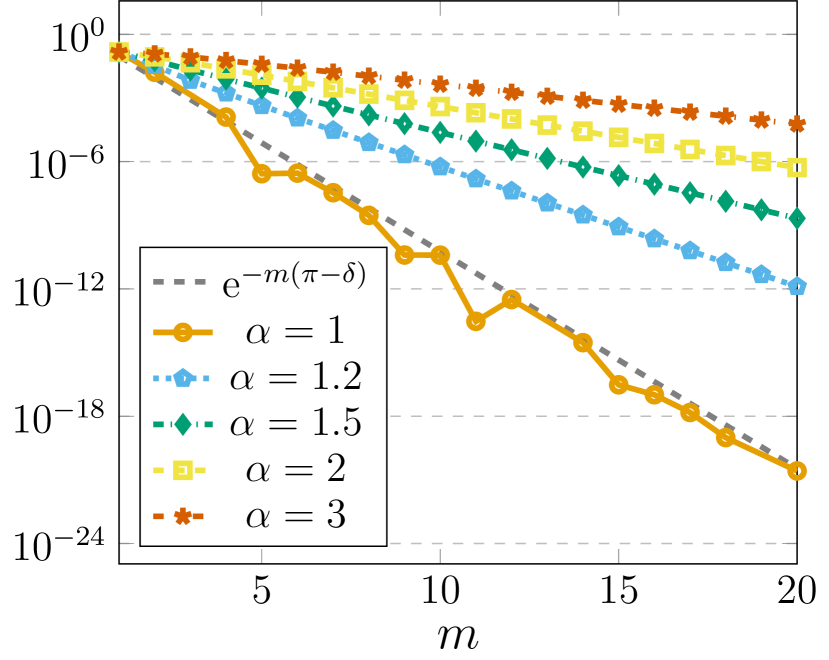
(a) $\delta=\frac{\pi}{4}$

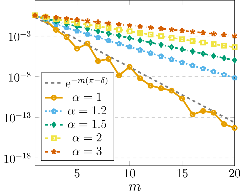
(b) $\delta=\frac{\pi}{2}$

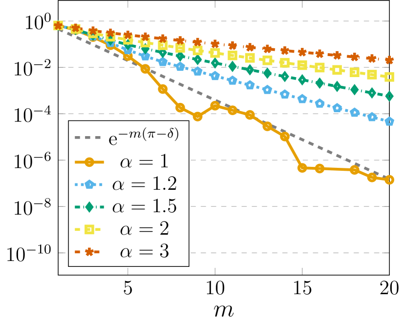
(c) $\delta=\frac{3\pi}{4}$

Figure 5.3: Semilogarithmic plots of the term $\frac{2\beta}{\pi\,\big{(}I_{0}(\beta)-1\big{)}}\,\int_{1/\alpha}^{\nu_{1}(0)}\Big{(}\frac{\sinh\big{(}\beta\,\sqrt{1-\nu^{2}}\big{)}}{\beta\,\sqrt{1-\nu^{2}}}-\frac{\sin(\beta\,\nu)}{\beta\,\nu}\Big{)}\,\mathrm{d}\nu$ for $m=1,\ldots,20$, $\alpha\in\{1.1,\,1.2,\,1.5,\,2,\,3\}$, and $\delta\in\big{\{}\frac{\pi}{4},\,\frac{\pi}{2},\,\frac{3\pi}{4}\big{\}}$.

(iii) On the other hand, we consider the expression (5.12) in the case

$$1<\alpha<\frac{\pi+\delta}{\pi-\delta}\,.$$

Then by (4.5) we have $\nu_{1}(\omega_{1})=1$ for $\omega_{1}\coloneqq\alpha\,(\pi-\delta)-\pi$. Without loss of generality, we can assume that $\omega_{1}\geq 0$. In the case $\omega_{1}>0$, we split the interval $[-\delta,\,\delta]$ into three subintervals $[-\delta,\,-\omega_{1}]$, $[-\omega_{1},\,\omega_{1}]$, and $[\omega_{1},\,\delta]$. In the case $\omega_{1}=0$, the interval $[-\delta,\,\delta]$ is decomposed into $[-\delta,\,0]$ and $[0,\,\delta]$. In the following, we discuss only the case $\omega_{1}>0$.

(A) For $\omega\in[-\delta,\,-\omega_{1}]$ we have again (4.20). Then from (5.12) and (5.3) it follows that

$$\Delta_{\mathrm{cKB},2}(\omega) =\frac{\beta}{m\,\sqrt{2\pi}}\,\bigg{(}\int_{1/\alpha}^{1}+\int_{1}^{\nu_{1}(-\omega)}+\int_{1/\alpha}^{\nu_{1}(\omega)}\bigg{)}\,{\hat{\varphi}}_{\mathrm{cKB}}\big{(}\tfrac{\beta}{m}\,\nu\big{)}\,{\mathrm{d}}\nu$$

$$=\frac{\beta}{\pi\,\big{(}I_{0}(\beta)-1\big{)}}\,\bigg{(}\int_{1/\alpha}^{1}+\int_{1/\alpha}^{\nu_{1}(\omega)}\bigg{)}\bigg{(}\frac{\sinh\big{(}\beta\,\sqrt{1-\nu^{2}}\big{)}}{\beta\,\sqrt{1-\nu^{2}}}-\frac{\sin(\beta\,\nu)}{\beta\,\nu}\bigg{)}\,\mathrm{d}\nu$$

$$\qquad+\,\frac{\beta}{\pi\,\big{(}I_{0}(\beta)-1\big{)}}\,\int_{1}^{\nu_{1}(-\omega)}\bigg{(}\frac{\sin\big{(}\beta\,\sqrt{\nu^{2}-1}\big{)}}{\beta\,\sqrt{\nu^{2}-1}}-\frac{\sin(\beta\,\nu)}{\beta\nu}\bigg{)}\,\mathrm{d}\nu\,,\quad\omega\in[-\delta,-\omega_{1}]\,.$$

Since the integrand (5.17) is nonnegative by Figure 5.2, using (4.20) and (5.8) implies that

$$\frac{\beta}{\pi\,\big{(}I_{0}(\beta)-1\big{)}}\,\int_{1/\alpha}^{1}\bigg{(}\frac{\sinh\big{(}\beta\,\sqrt{1-\nu^{2}}\big{)}}{\beta\,\sqrt{1-\nu^{2}}}-\frac{\sin(\beta\nu)}{\beta\nu}\bigg{)}\,\mathrm{d}\nu<\big{|}\Delta_{\mathrm{cKB},2}(\omega)\big{|}$$

$$\qquad<\,\frac{2\beta}{\pi\,\big{(}I_{0}(\beta)-1\big{)}}\,\int_{1/\alpha}^{1}\bigg{(}\frac{\sinh\big{(}\beta\,\sqrt{1-\nu^{2}}\big{)}}{\beta\,\sqrt{1-\nu^{2}}}-\frac{\sin(\beta\nu)}{\beta\nu}\bigg{)}\,\mathrm{d}\nu$$

$$\qquad\qquad+\,\frac{\beta}{\pi\,\big{(}I_{0}(\beta)-1\big{)}}\,\int_{1}^{\nu_{1}(-\omega)}\bigg{|}\frac{\sin\big{(}\beta\,\sqrt{1-\nu^{2}}\big{)}}{\beta\,\sqrt{1-\nu^{2}}}-\frac{\sin(\beta\nu)}{\beta\nu}\bigg{|}\,\mathrm{d}\nu$$

$$\qquad\leq\frac{2\beta}{\pi\,\big{(}I_{0}(\beta)-1\big{)}}\,\int_{1/\alpha}^{1}\bigg{(}\frac{\sinh\big{(}\beta\,\sqrt{1-\nu^{2}}\big{)}}{\beta\,\sqrt{1-\nu^{2}}}-\frac{\sin(\beta\nu)}{\beta\nu}\bigg{)}\,\mathrm{d}\nu+\frac{2\beta}{\pi\,\big{(}I_{0}(\beta)-1\big{)}}\,.$$

We remark that by $\beta=\alpha\,m\,(\pi-\delta)$ with $\alpha>1$ and $0<\delta\leq\frac{m-1}{m}\,\delta$ we have $\beta>\pi$, and hence by (5.9) this yields

$$\frac{1}{I_{0}(\beta)-1}<\frac{7}{4}\,\beta\,\mathrm{e}^{-\beta}\,.$$

Numerical experiments, cf. Figure 5.4, have shown that

$$\frac{2\beta}{\pi\,\big{(}I_{0}(\beta)-1\big{)}}\,\int_{1/\alpha}^{1}\bigg{(}\frac{\sinh\big{(}\beta\,\sqrt{1-\nu^{2}}\big{)}}{\beta\,\sqrt{1-\nu^{2}}}-\frac{\sin(\beta\nu)}{\beta\nu}\bigg{)}\,\mathrm{d}\nu\,,\quad\alpha>1\,,$$

tends to zero as $m\to\infty$ with exponential decay smaller than $m\,(\pi-\delta)$. Therefore, we obtain that

$$\max_{\omega\in[-\delta,-\omega_{1}]}\big{|}\Delta_{\mathrm{cKB},2}(\omega)\big{|}$$

tends to zero as $m\to\infty$ with exponential decay smaller than $m\,(\pi-\delta)$.

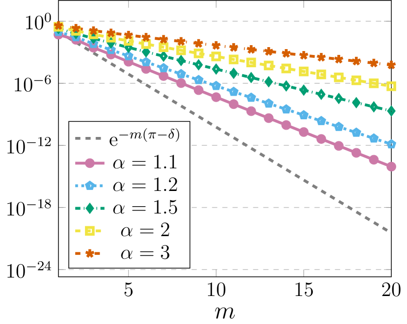
(a) $\delta=\frac{\pi}{4}$

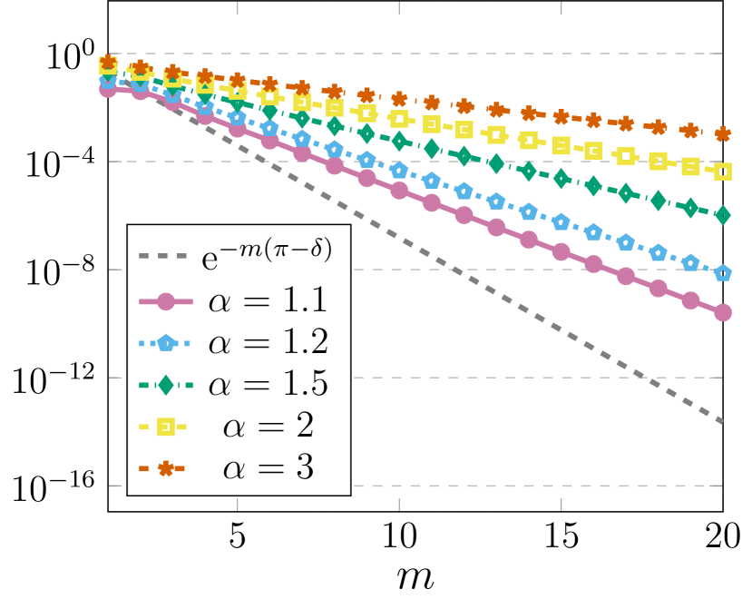
(b) $\delta=\frac{\pi}{2}$

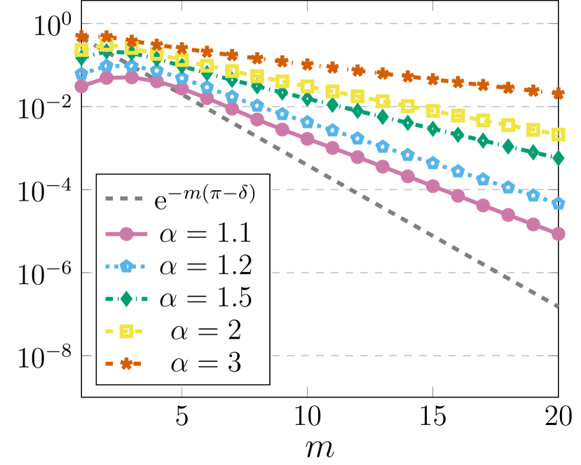
(c) $\delta=\frac{3\pi}{4}$

Figure 5.4: Semilogarithmic plots of the term $\frac{2\beta}{\pi\,\big{(}I_{0}(\beta)-1\big{)}}\,\int_{1/\alpha}^{1}\Big{(}\frac{\sinh\big{(}\beta\,\sqrt{1-\nu^{2}}\big{)}}{\beta\,\sqrt{1-\nu^{2}}}-\frac{\sin(\beta\nu)}{\beta\nu}\Big{)}\,\mathrm{d}\nu$ for $m=1,\ldots,20$, $\alpha\in\{1.1,\,1.2,\,1.5,\,2,\,3\}$, and $\delta\in\big{\{}\frac{\pi}{4},\,\frac{\pi}{2},\,\frac{3\pi}{4}\big{\}}$.

(B) For $\omega\in[-\omega_{1},\,\omega_{1}]$ we have again (4.21). Then from (5.12) and (5.3) it follows that for $\omega\in[-\omega_{1},\,\omega_{1}]$ we have

$$\Delta_{\mathrm{cKB},2}(\omega) =\frac{\beta}{m\,\sqrt{2\pi}}\,\bigg{(}\int_{1/\alpha}^{\nu_{1}(-\omega)}+\int_{1/\alpha}^{\nu_{1}(\omega)}\bigg{)}\,{\hat{\varphi}}_{\mathrm{cKB}}\big{(}\tfrac{\beta}{m}\,\nu\big{)}\,{\mathrm{d}}\nu$$

$$=\frac{\beta}{\pi\,\big{(}I_{0}(\beta)-1\big{)}}\,\bigg{(}\int_{1/\alpha}^{\nu_{1}(-\omega)}+\int_{1/\alpha}^{\nu_{1}(\omega)}\bigg{)}\bigg{(}\frac{\sinh\big{(}\beta\,\sqrt{1-\nu^{2}}\big{)}}{\beta\,\sqrt{1-\nu^{2}}}-\frac{\sin(\beta\nu)}{\beta\nu}\bigg{)}\,\mathrm{d}\nu\,.$$

Note that by (4.5) and (4.21) we have again (4.16) and therefore (5.16) holds for $\omega\in[0\,,\omega_{1}]$. Analogous to step (ii) this implies

$$\max_{\omega\in[-\omega_{1},\omega_{1}]}\Delta_{\mathrm{cKB},2}(\omega)=\frac{\beta}{\pi\,\big{(}I_{0}(\beta)-1\big{)}}\,\int_{1/\alpha}^{\nu_{1}(0)}\bigg{(}\frac{\sinh(\beta\sqrt{1-\nu^{2}})}{\beta\,\sqrt{1-\nu^{2}}}-\frac{\sin(\beta\nu)}{\beta\nu}\bigg{)}\,\mathrm{d}\nu\,.$$

Hence, by the numerical experiments in Figure 5.3 we see that

$$\max_{\omega\in[-\omega_{1},\omega_{1}]}\Delta_{\mathrm{cKB},2}(\omega)$$

tends to zero as $m\to\infty$ with exponential decay smaller than $m\,(\pi-\delta)$.

(C) For $\omega\in[\omega_{1},\,\delta]$ we have again (4.22). Then from (5.12) and (5.3) it follows that

$$\Delta_{\mathrm{cKB},2}(\omega) =\frac{\beta}{m\,\sqrt{2\pi}}\,\bigg{(}\int_{1/\alpha}^{\nu_{1}(-\omega)}+\int_{1/\alpha}^{1}+\int_{1}^{\nu_{1}(\omega)}\bigg{)}\,{\hat{\varphi}}_{\mathrm{cKB}}\big{(}\tfrac{\beta}{m}\,\nu\big{)}\,{\mathrm{d}}\nu$$

$$=\frac{\beta}{\pi\,\big{(}I_{0}(\beta)-1\big{)}}\,\bigg{(}\int_{1/\alpha}^{\nu_{1}(-\omega)}+\int_{1/\alpha}^{1}\bigg{)}\bigg{(}\frac{\sinh\big{(}\beta\,\sqrt{1-\nu^{2}}\big{)}}{\beta\,\sqrt{1-\nu^{2}}}-\frac{\sin(\beta\nu)}{\beta\nu}\bigg{)}\,\mathrm{d}\nu$$

$$\qquad+\,\frac{\beta}{\pi\,\big{(}I_{0}(\beta)-1\big{)}}\,\int_{1}^{\nu_{1}(\omega)}\bigg{(}\frac{\sin\big{(}\beta\,\sqrt{\nu^{2}-1}\big{)}}{\beta\,\sqrt{\nu^{2}-1}}-\frac{\sin(\beta\nu)}{\beta\nu}\bigg{)}\,\mathrm{d}\nu\,.$$

Since the integrand (5.17) is nonnegative by Figure 5.2, using (4.22), (5.8) and (5.9) for the shape parameter $\beta=\alpha\,m\,(\pi-\delta)>\alpha\,\pi>\pi$ implies

$$\frac{\beta}{\pi\,\big{(}I_{0}(\beta)-1\big{)}}\,\int_{1/\alpha}^{1}\bigg{(}\frac{\sinh\big{(}\beta\,\sqrt{1-\nu^{2}}\big{)}}{\beta\,\sqrt{1-\nu^{2}}}-\frac{\sin(\beta\nu)}{\beta\nu}\bigg{)}\,\mathrm{d}\nu<\big{|}\Delta_{\mathrm{cKB},2}(\omega)\big{|}$$

$$\qquad<\,\frac{2\beta}{\pi\,\big{(}I_{0}(\beta)-1\big{)}}\,\int_{1/\alpha}^{1}\bigg{(}\frac{\sinh\big{(}\beta\,\sqrt{1-\nu^{2}}\big{)}}{\beta\,\sqrt{1-\nu^{2}}}-\frac{\sin(\beta\nu)}{\beta\nu}\bigg{)}\,\mathrm{d}\nu$$

$$\qquad\qquad+\frac{\beta}{\pi\,\big{(}I_{0}(\beta)-1\big{)}}\,\int_{1}^{\nu_{1}(\omega)}\bigg{|}\frac{\sin\big{(}\beta\,\sqrt{\nu^{2}-1}\big{)}}{\beta\,\sqrt{\nu^{2}-1}}-\frac{\sin(\beta\nu)}{\beta\nu}\bigg{|}\,\mathrm{d}\nu$$

$$\qquad<\,\frac{2\beta}{\pi\,\big{(}I_{0}(\beta)-1\big{)}}\,\int_{1/\alpha}^{1}\bigg{(}\frac{\sinh\big{(}\beta\,\sqrt{1-\nu^{2}}\big{)}}{\beta\,\sqrt{1-\nu^{2}}}-\frac{\sin(\beta\nu)}{\beta\nu}\bigg{)}\,\mathrm{d}\nu+\frac{7}{2\pi}\,\beta^{2}\,\mathrm{e}^{-\beta}\,.$$

Hence, by the numerical experiments in Figure 5.4 we obtain that

$$\max_{\omega\in[\omega_{1},\delta]}\big{|}\Delta_{\mathrm{cKB},2}(\omega)\big{|}$$

tends to zero as $m\to\infty$ with exponential decay smaller than $m\,(\pi-\delta)$.

In summary,

$$D_{2}(m)=\max_{\omega\in[-\delta,\delta]}\big{|}\Delta_{\mathrm{cKB},2}(\omega)\big{|}$$

tends to zero for $m\to\infty$ with exponential decay smaller than $m\,(\pi-\delta)$.  

Example 5.3.

Analogous to Example 4.4 we now visualize the optimality of the shape parameter $\beta=m\,(\pi-\delta)$ for the continuous Kaiser–Bessel regularized Shannon sampling formula shown in Theorems 5.1 and 5.2. More precisely, for the bandlimited function (3.8) with several bandwidth parameters $\delta\in\big{\{}\frac{\pi}{4},\,\frac{\pi}{2},\,\frac{3\pi}{4}\big{\}}$, i. e., several oversampling rates $\frac{\pi}{\delta}>1$, we consider the regularized Shannon sampling formula (1.4) with the continuous Kaiser–Bessel window function $\varphi_{\mathrm{cKB}}$ in (1.8). The corresponding approximation error (3.7) shall again be approximated by evaluating the given function $f$ and its approximation $R_{\varphi,m}f$ at equidistant points $t_{s}\in[-1,\,1]$, $s=1,\dots,S$, with $S=10^{5}$. To compare with the optimal parameter, we choose the shape parameter of the continuous Kaiser–Bessel window function (1.8) as $\beta=\alpha\,m\,(\pi-\delta)$ with $\alpha\in\big{\{}\frac{1}{2},1,2\big{\}}$.

The results for different truncation parameters $m\in\{2,3,\ldots,10\}$ are depicted in Figure 5.5. As stated in Theorem 5.2, it can clearly be seen that the choice of $\alpha\neq 1$ causes worsened error decay rates with respect to $m$. Thus, the numerical results confirm that the shape parameter $\beta=m\,(\pi-\delta)$ of Theorem 5.1 is optimal, and that this fact can already be observed for very small truncation parameters $m\in\mathbb{N}\setminus\{1\}$.

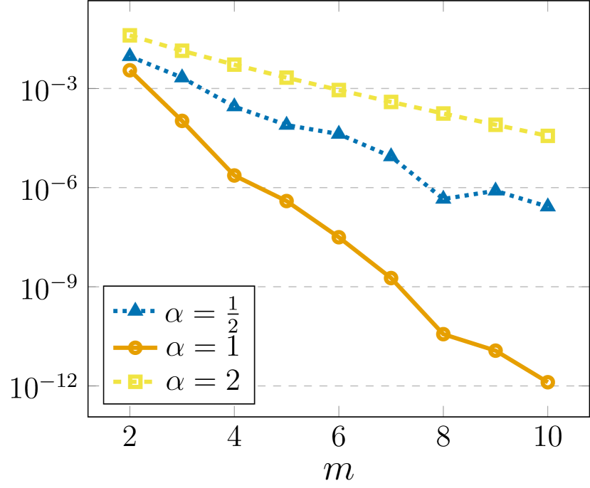
(a) $\delta=\frac{\pi}{4}$

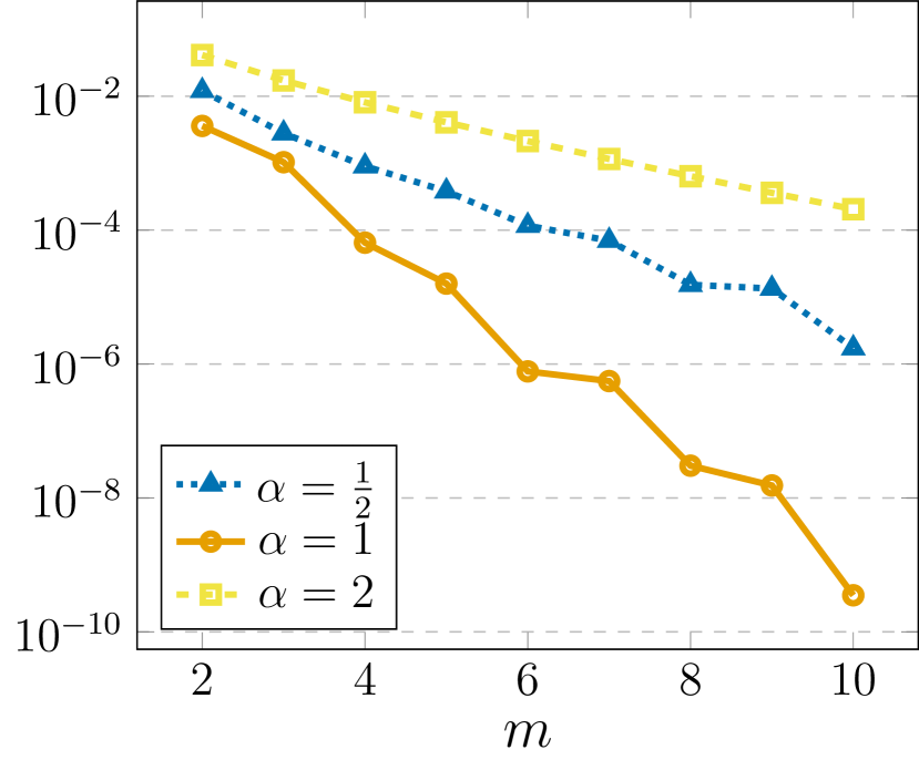
(b) $\delta=\frac{\pi}{2}$

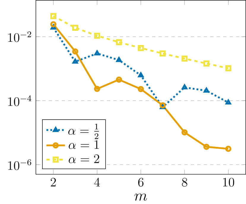
(c) $\delta=\frac{3\pi}{4}$

Figure 5.5: Maximum approximation error (3.7) using the continuous Kaiser–Bessel window function $\varphi_{\mathrm{cKB}}$ in (1.8) with different shape parameters $\beta=\alpha\,m(\pi-\delta)$, $\alpha\in\big{\{}\frac{1}{2},1,2\big{\}}$, for the bandlimited function (3.8) with bandwidths $\delta\in\big{\{}\frac{\pi}{4},\frac{\pi}{2},\frac{3\pi}{4}\big{\}}$ and truncation parameters $m\in\{2,3,\ldots,10\}$.

      

We further remark that already in [13, Theorem 4.3] bounds on the approximation error of the Shannon sampling formula (1.4) were shown for the continuous Kaiser–Bessel window function (1.8) with suitably chosen shape parameter $\beta$. However, in this previous work the optimal parameter was only conjectured by numerical testing, whereas the proof of the optimality was still an open problem. Note that although the respective parameter looks different than the one in Theorem 5.1, it is basically the same, only adapted to the slightly different setting considered in [13]. Therefore, the newly proposed Theorem 5.2 provides not only a proof for the optimality of the parameter choice in Theorem 5.1 but also for the parameter choice of [13].

Remark 5.4.

Note that the code files for this and all the other experiments are available on https://github.com/melaniekircheis/Optimal-parameter-choice-for-regularized-Shannon-sampling-formulas.       

6 Conclusion

In this paper, we have studied the regularized Shannon sampling formula (1.4) for the widely used Gaussian function (1.5), the modified Gaussian function (1.6), the $\sinh$-type window function (1.7), and the continuous Kaiser–Bessel window function (1.8). More precisely, for an arbitrary bandlimited function $f\in L^{2}(\mathbb{R})\cap C(\mathbb{R})$ with bandwidth $\delta\in(0,\,\pi)$ we have shown that the uniform approximation error (1.10) of the regularized Shannon sampling formulas of $f$ possess an exponential decay with respect to the truncation parameter $m$. In doing so, we have demonstrated that the decay rate $m\,(\pi-\delta)$ of the $\sinh$-type regularized Shannon sampling formula, see Theorem 4.1, and the continuous Kaiser–Bessel regularized Shannon sampling formula, see Theorem 5.1, is much better than the decay rate $m\,(\pi-\delta)/2$ of the Gaussian regularized Shannon sampling formula, see Theorem 3.1. Note that the $\sinh$-type regularized Shannon sampling formula is even better than the continuous Kaiser–Bessel regularized Shannon sampling formula due to the constant factors in (4.1) and (5.1), see also Figure 6.1.

Moreover, we found that the exponential decay of the approximation error of the regularized Shannon sampling formula (1.4) strongly depends on the shape parameter of the corresponding window function. Namely, the optimal choice of the variance $\sigma^{2}$ of the (modified) Gaussian function and of the shape parameter $\beta$ of the $\sinh$-type window function and the continuous Kaiser–Bessel function is a crucial ingredient for a fast and accurate reconstruction of $f$. Therefore, the main focus of this paper was to determine the optimal variances $\sigma^{2}$ in Theorems 3.1 and 3.4 as well as the optimal shape parameters $\beta$ in Theorems 4.2 and 5.2, such that the exponential decay of the approximation error (1.10) is as large as possible. These results further emphasize the superiority of the $\sinh$-type regularized Shannon sampling formula of $f$, since the approximation errors of the regularized Shannon sampling formulas were compared for the optimal shape parameters each.

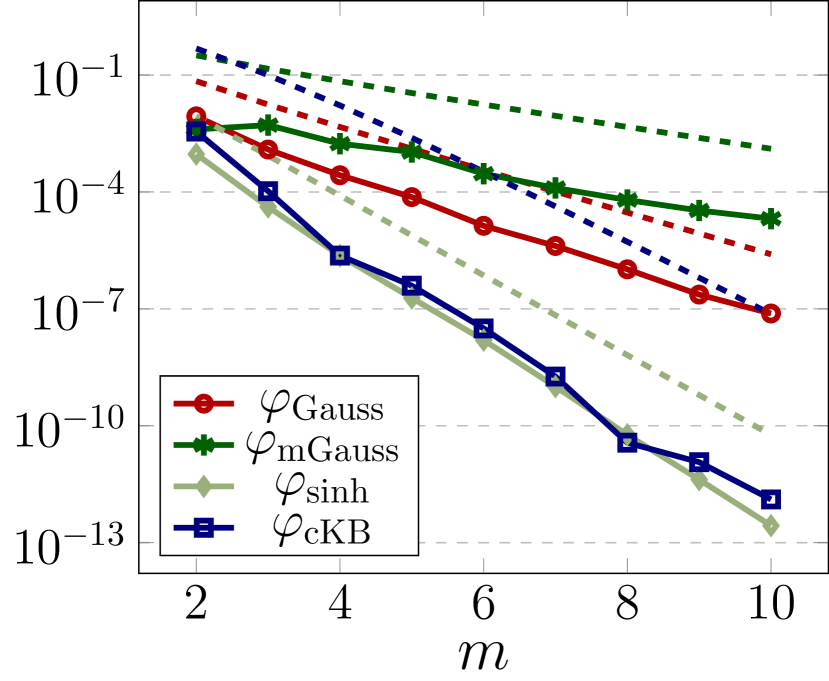
(a) $\delta=\frac{\pi}{4}$

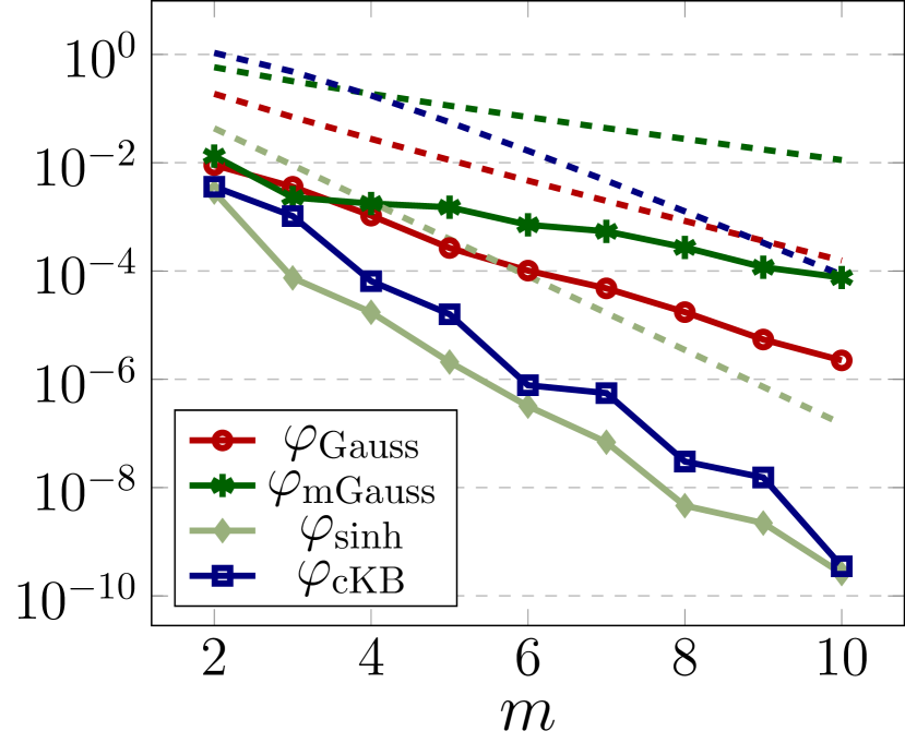
(b) $\delta=\frac{\pi}{2}$

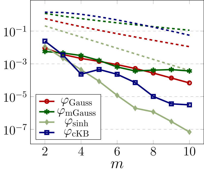
(c) $\delta=\frac{3\pi}{4}$

Figure 6.1: Maximum approximation error (3.7) (solid) and error constants (dashed) using $\varphi\in\{\varphi_{\mathrm{Gauss}},\varphi_{\mathrm{mGauss}},\varphi_{\sinh},\varphi_{\mathrm{cKB}}\}$, see (1.5), (1.6), (1.7), and (1.8), for the bandlimited function (3.8) with $\delta\in\big{\{}\frac{\pi}{4},\,\frac{\pi}{2},\,\frac{3\pi}{4}\big{\}}$ and $m\in\{2,3,\ldots,10\}$.

References

[1]
M. Abramowitz and I.A. Stegun, editors.
Handbook of Mathematical Functions with Formulas, Graphs, and Mathematical Tables.
Dover, New York, 1972.
[2]
Á. Baricz and T.K. Pogány.
Functional inequalities for modified Struve functions II.
Math. Inequal. Appl., 17:1387–1398, 2014.
[3]
A. H. Barnett.
Aliasing error of the kernel in the nonuniform fast Fourier transform.
Appl. Comput. Harmon. Anal., 51:1–16, 2021.
[4]
A. H. Barnett, J. F. Magland, and L. A. Klinteberg.
Flatiron Institute nonuniform fast Fourier transform libraries (FINUFFT).
http://github.com/flatironinstitute/finufft.
[5]
L. Chen and H. Zhang.
Sharp exponential bounds for the Gaussian regularized Whittaker–Kotelnikov–Shannon sampling series.
J. Approx. Theory, 245:73–82, 2019.
[6]
I. Daubechies.
Ten Lectures on Wavelets.
SIAM, Philadelphia, 1992.
[7]
I. Daubechies and R. DeVore.
Approximating a bandlimited function using very coarsely quantized data: A family of stable sigma-delta modulators of arbitrary order.
Ann. of Math. (2), 158:679–710, 2003.
[8]
H. G. Feichtinger.
New results on regular and irregular sampling based on Wiener amalgams.
In K. Jarosz, editor, Function Spaces, Proc Conf, Edwardsville/IL (USA) 1990, volume 136 of Lect. Notes Pure Appl. Math.,pages 107––121. New York, 1992.
[9]
H. G. Feichtinger.
Wiener amalgams over Euclidean spaces and some of their applications.
In K. Jarosz, editor, Function Spaces, Proc Conf, Edwardsville/IL (USA) 1990, volume 136 of Lect. Notes Pure Appl. Math., pages 123––137. New York, 1992.
[10]
I.S. Gradshteyn and I.M. Ryzhik.
Table of Integrals, Series, and Products.
Academic Press, New York, 1980.
[11]
D. Jagerman.
Bounds for truncation error of the sampling expansion.
SIAM J. Appl. Math., 14(4):714–723, 1966.
[12]
M. Kircheis, D. Potts, and M. Tasche.
On regularized Shannon sampling formulas with localized sampling.
Sampl. Theory Signal Process. Data Anal., 20: Paper No. 20, 34 pp., 2022.
[13]
M. Kircheis, D. Potts, and M. Tasche.
On numerical realizations of Shannon’s sampling theorem.
Sampl. Theory Signal Process. Data Anal., 22: Paper No. 13, 33 pp., 2024.
[14]
V. A. Kotelnikov.
On the transmission capacity of the ether and wire in
electrocommunications.
In J.J. Benedetto and P.J.S.G. Ferreira (eds.) Modern Sampling Theory: Mathematics and Application, pages
27–45. Birkhäuser, Boston, 2001.
Translated from Russian.
[15]
R. Lin and H. Zhang.
Convergence analysis of the Gaussian regularized Shannon sampling formula.
Numer. Funct. Anal. Optim., 38(2):224–247, 2017.
[16]
C.A. Micchelli, Y. Xu, and H. Zhang.
Optimal learning of bandlimited functions from localized sampling.
J. Complexity, 25(2):85–114, 2009.
[17]
F. Natterer.
Efficient evaluation of oversampled functions.
J. Comput. Appl. Math., 14(3):303–309, 1986.
[18]
F. Oberhettinger.
Tables of Fourier Transforms and Fourier Transforms of Distributions.
Springer, Berlin, 1990.
[19]
J. R. Partington.
Interpolation, Identification, and Sampling.
Clarendon Press, New York, 1997.
[20]
G. Plonka, D. Potts, G. Steidl, and M. Tasche.
Numerical Fourier Analysis.
Second edition, Birkhäuser/Springer, Cham, 2023.
[21]
D. Potts and M. Tasche.
Continuous window functions for NFFT.
Adv. Comput. Math. 47(2): Paper 53, 34 pp., 2021.
[22]
L. Qian.
On the regularized Whittaker–Kotelnikov–Shannon sampling formula.
Proc. Amer. Math. Soc., 131(4):1169–1176, 2003.
[23]
L. Qian.
The regularized Whittaker-Kotelnikov-Shannon sampling theorem and its application to the numerical solutions of partial differential equations.
PhD thesis, National Univ. Singapore, 2004.
[24]
L. Qian and D.B. Creamer.
Localization of the generalized sampling series and its numerical application.
SIAM J. Numer. Anal. 43(6):2500–2516, 2006.
[25]
L. Qian and H. Ogawa.
Modified sinc kernels for the localized sampling series.
Sampl. Theory Signal Image Process. 4(2):121–139, 2005.
[26]
T. S. Rappaport.
Wireless Communications: Principles and Practice.
Prentice Hall, New Jersey, 1996.
[27]
G. Schmeisser and F. Stenger.
Sinc approximation with a Gaussian multiplier.
Sampl. Theory Signal Image Process., 6(2):199–221, 2007.
[28]
C. E. Shannon.
Communication in the presence of noise.
Proc. I.R.E., 37:10–21, 1949.
[29]
T. Strohmer and J. Tanner.
Fast reconstruction methods for bandlimited functions from periodic nonuniform sampling.
SIAM J. Numer. Anal., 44(3):1071-1094, 2006.
[30]
K. Tanaka, M. Sugihara, and K. Murota.
Complex analytic approach to the sinc-Gauss sampling formula.
Japan J. Ind. Appl. Math., 25:209–231, 2008.
[31]
E.T. Whittaker.
On the functions which are represented by the expansions of the
interpolation theory.
Proc. R. Soc. Edinb., 35:181–194, 1915.