-deformed evolutionary dynamics in simple matrix games
Abstract
We consider evolutionary games in which the agent selected for update compares their payoff to neighbours, rather than a single neighbour as in standard evolutionary game theory. Through studying fixed point stability and fixation times for games with all-to-all interactions, we find that the flow changes significantly as a function of . Further, we investigate the effects of changing the underlying topology from an all-to-all interacting system to an uncorrelated graph via the pair approximation. We also develop the framework for studying games with more than two strategies, such as the rock-paper-scissors game where we show that changing leads to the emergence of new types of flow.
I Introduction
Modern game theory was pioneered by mathematician John von Neumann in the 1920s to mathematically model strategic interactions among agents whose decisions are rational [1, 2, 3]. In the 1970s John Maynard Smith and George Price built on this idea by introducing evolutionary game theory [4, 5]. Here, agents do not act rationally, instead each individual carries a particular strategy that is passed on from parent to offspring. Reproduction occurs in proportion to fitness. This was initially conceived as a model of Darwinian evolution in biology, but has also found applications in the social sciences and in economics [6]. Originally, evolutionary game dynamics in populations were described mostly by deterministic differential equations, such as the commonly used replicator equations [7]. These equations are formally valid for infinite populations.
However, it is now well established that stochastic effects can considerably affect the outcome of evolution (see e.g. [8, 9, 10]). There is thus a continuously growing body of work on evolutionary game theory in finite populations. One particular focus is also on networked populations, that is, population in which any one individual can only interact and compete with its immediate neighbours. This has sometimes been referred to as ‘evolutionary graph theory’ [11]. This should should not be misunderstood as a theory of evolving graphs. Despite the terminology, the underlying graph does often not change in time.
The starting point for studies of evolutionary game theory in finite populations and networks is usually an individual-based model. This is a set of rules by which the agents interact and the population evolves. A number of different interaction models have been proposed, see e.g. [12, 13]; a summary can also be found in [14]. For analytical convenience the total size of the population is often kept fixed. Here, we focus on the so-called pairwise comparison process mediated via ‘Fermi functions’ [15]. Detailed definitions will be given in Sec. II.
The so-called voter model is a related, but different model of interacting individuals. It was originally introduced by Holley and Liggett in 1975 to model interacting particle systems [16]. In the most basic voter model, the population consists of voters which are of binary types (‘opinions’), 0 or 1, connected in some way through a network. In each step of the dynamics one randomly chosen individual adopts the opinion of a randomly chosen neighbour. Many extensions and variations of this model have been proposed and studied [17, 18, 19, 20, 21]. One such variation is the so-called ‘-voter model’, in which neighbours need to agree with one another in order for a voter to change opinion [22, 23, 24].
In this paper we seek to combine the ideas of evolutionary games and the -voter model into ‘-deformed’ evolutionary game dynamics. We consider a population of individuals who each carry a particular strategy, and the population then evolves following rules similar to those in conventional models of evolutionary game theory, in particular the probability for an agent to change state depends on payoff. However, before a change can occur, an agent must consult with of its neighbours. As in the -voter model a change of that agent can then only occur if all those neighbours are of the same type. As we will show this can significantly affect the evolutionary flow in strategy space, and quantities such as fixation probabilities and times in finite populations.
The remainder of the paper is organised as follows. In Sec. II we introduce the model of -deformed evolutionary game dynamics for games (two-strategy two-player games). In Sec. III we investigate the rate equations for the -deformed dynamics in infinite all-to-all populations. We study the fixed points and their stability, and show that the type of evolutionary flow changes as a function of . In Sec. IV we look at fixation times and probabilities in finite all-to-all systems. In Sec. V we study the effects of changing the underlying topology from a complete graph to an uncorrelated graph. Analytical results for -deformed dynamics are obtained within the pair approximation. In Sec. VI we study games with more than two strategies. We investigate cyclic games (motivated by the familiar rock-paper-scissors game) as an example and show that -deformation can induce new behaviour, in particular the emergence of stable limit cycles. Finally in Sec. VII we look at a modified version of the model, where we select the -neighbours without replacement. We summarise our results in Sec. VIII, and give an outlook on possible future work.
II Model definitions
II.1 Payoff matrix
We consider a population of agents, who are each of type or . For the time being we always consider a population with all-to-all interaction.
The game is defined by the payoff matrix
| (1) |
An agent interacting with another agent thus receives payoff , and it receives if interacting with an agent of type . Likewise a agent receives when interacting with an , and when interacting with a .
In finite systems we characterise the state by the number of type agents , or, equivalently, by the fraction of agents in the population, . The expected payoff for type and agents respectively is then
| (2) |
We can define the payoff difference as
| (3) |
where,
| (4) |
For evolutionary processes relying only on payoff differences it is thus possible to represent the payoff matrix in Eq. (1) with only two variables: and .
II.2 -deformed evolutionary dynamics
At each time step we randomly choose an agent for update, say it is of type . We then choose agents from the population (with replacement). If all those agents are of type , then the switches to , with a probability that depends on the payoffs of type and agents. Similarly, we write for the probability for a to switch to if other randomly selected agents also are of type .
There are many possible choices for the functions . One such choice is to make proportional to the payoff of the type that is being switched to, i.e.
| (5) |
This choice is is only valid if all entries in the payoff matrix are positive. The denominator ensures that . In this way, if type agents have a large average payoff, then type agents are likely to switch during interactions with them. But it is still possible for an agent to switch to a type with a lower expected payoff than its current type. A second popular choice involves non-linear Fermi functions [25, 15],
| (6) |
These depend on the payoff difference. The parameter , known as the intensity of selection, reflects the uncertainty in decision-making processes. In the strong selection limit, an individual will always switch to the type with the higher expected payoff. For any finite the reverse process occurs with non-zero probability. For one has , i.e. neutral selection. Payoffs then have no effect. Since the parameter only appears in combination with and , we will absorb it into those parameters, effectively setting .
The rates at which the type and agents switch are given by,
| (7) |
respectively. The first expression can be understood as follows. The agent chosen for reproduction is of type with probability . The probability that randomly chosen neighbours (with replacement) in this all-to-all population are all of type is . The type agent switches to type with probability . We will sometimes write instead of , noting that .
We measure time in units of generations, the rates are therefore proportional to the size of the population. While the above motivation of the model implicitly assumes that is a positive integer, the continuous-time rates in Eq. (7) are mathematically meaningful for all . We thus treat as a real-valued model parameter, similar to what is done in the literature on the -voter model [26, 23, 27, 28, 29, 24]. For the setup reduces to that of conventional evolutionary game theory in finite populations (see e.g. [10, 9, 30, 14]). We will refer to choices as a ‘-deformation’ of the dynamics.
It is easy to understand that -deformation favours strategies that are in the minority when , or in majority respectively, for . To see this it is useful to focus on the case with no selection ( in our notation). If the frequency of strategy is , the rate of change from to is proportional to and that for the reverse change proportional to . For these terms balance for all . This is the case of the conventional voter model, where there is no deterministic drift. For we have when . Thus for strategy is favoured when it is in the minority, and disfavoured when more than half of population is of type . The direction of the flow reverses for .
III Rate equations for infinite populations
III.1 -deformed rate equations
For large populations the average dynamics of the population is approximated by a -deformed version of the conventional rate equations in an infinite population. This is explained further in the Supplemental Material (SM) [31], see in particular Sec. S1. We have
| (8) |
The quantity in this equation is really , an average over individual realisations of the dynamics. However to ease notation we will write throughout. Also note if we choose as in Eq. (5), then after absorbing the constant by re-scaling time we find,
| (9) |
This is a -deformed variant of the conventional replicator equations. Setting reduces this to the standard replicator equation for -player -strategy games [32],
| (10) |
Given an initial distribution of type and agents in a population, Eq. (8) determines how the composition of the population changes with time. The system will eventually reach a fixed point. The location of the fixed point depends on and , and (potentially) on the initial condition. Our first step is therefore an analysis of the fixed points of the -deformed rate equations and of the stability of these fixed points. As a benchmark we first summarise the well-known results for the case .
III.2 The case
The simplest case is that of , where Eq. (8) reduces to
| (11) |
In this case, there are always two fixed points at the boundaries, . There is also potentially a third, interior, fixed point given by the solution of . For the functions in Eqs. (5) and (6), this equates to solving , so
| (12) |
For some values of and this solution is unphysical ( or ). We then only have the fixed points at and . In the special case and (neutral selection) we have , in which case every point is a fixed point.
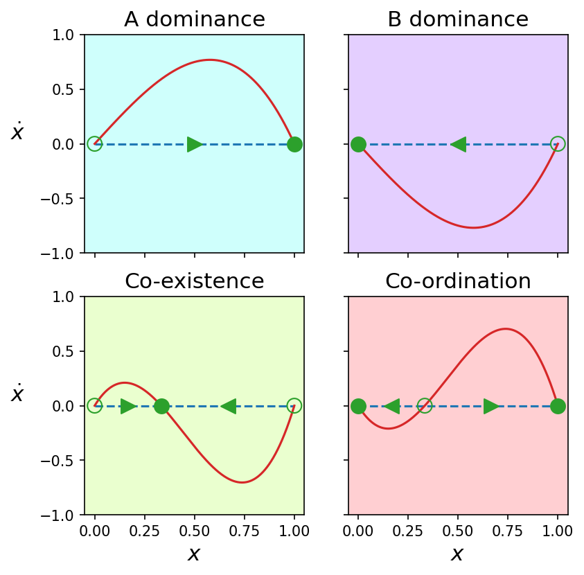
Given values for and we can characterise the type of flow based on the number of fixed points and their linear stability. From Eq. (11), if then is unstable. If then is a stable fixed point. If an interior fixed point exists, it is stable if
| (13) |
These scenarios are summarised in Fig. 1. They are conventionally referred to as the dominance of or , ‘co-existence’ or ‘co-ordination’, respectively [10].
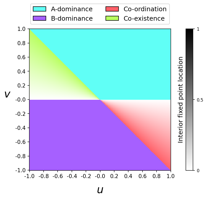
We can create a phase diagram in the (,)-space to demonstrate how the evolutionary flow changes when we alter the payoff matrix. Fig. 2 shows how this space divides into four regions with the four types of flow. The diagram is valid for the choices of in Eqs. (5) and (6). In the case of co-existence or co-ordination, the interior fixed point can vary on the interval which is represented by the opacity of those regions. The shape of these regions can be explained as follows. We have one interior fixed point when and from Eq. (12) this implies . When we find that and , this defines the red region in Fig. 2. We then evaluate Eq. (13) at , to find that means that the interior fixed point is unstable, hence one has co-ordination type flow [Fig. 1]. Similar analyses can be carried out for the other regions. We note here how the co-existence and co-ordination games blend into dominance games as we change and , since their interior fixed points move closer the the boundaries, eventually being absorbed.
III.3 The case
We now focus on the case in Eq. (8). Much like the case we always have fixed points at the boundaries, and . The number of interior fixed points depends on the functions .
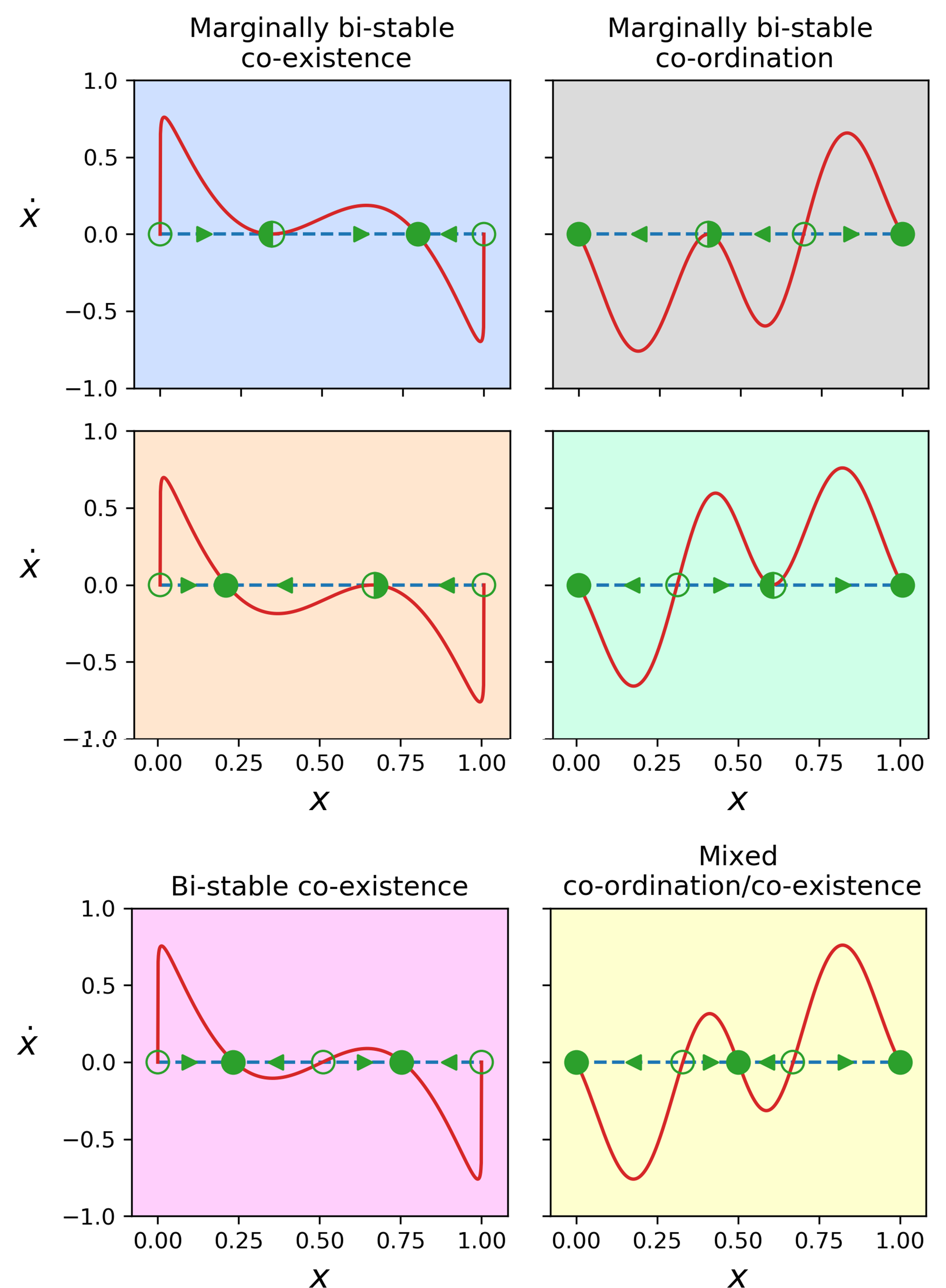
All results in this section are for the Fermi function Eq. (6). We find that there can be between one and three interior fixed points. For , we only find co-ordination type flows (i.e. flows with stable fixed points at the boundaries), and for we only find co-existence type flows (i.e. flows with unstable fixed points at the boundaries) [see SM, Sec. S2]. This is because the -deformation favours majority strategies for , while the minority strategy has an advantage for . The possible types of flow of Eq. (8) include standard co-ordination and co-existence as shown in Fig. 1 and the additional types shown in Fig. 3. The left column shows co-existence type behaviour. The right column shows co-ordination type dynamics.
Even though mathematically we might classify a flow as co-ordination, co-existence or one of the new types, the interior fixed point(s) are often close to or . The behaviour is then more like a dominance scenario. It is often insightful to plot as a function of for specific parameters , and .
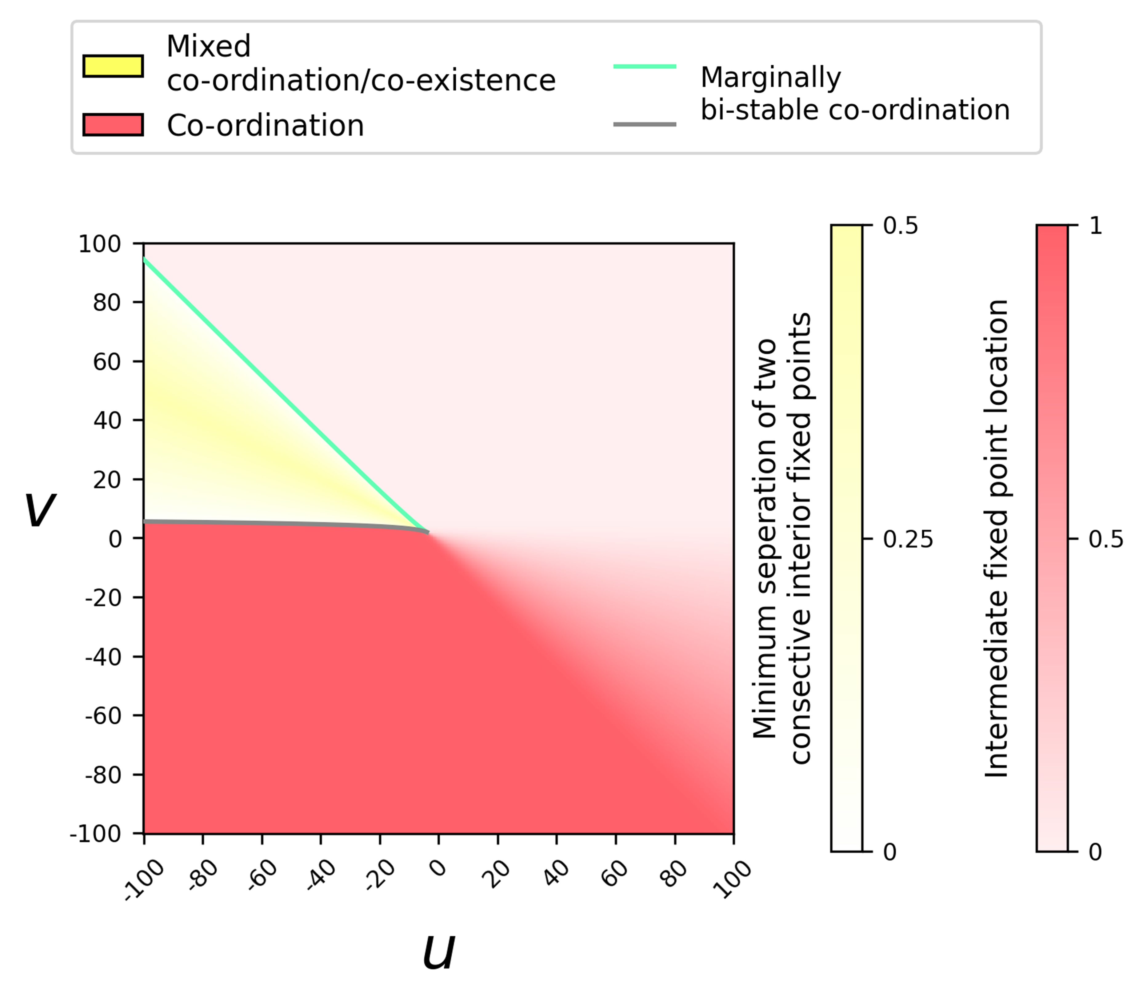
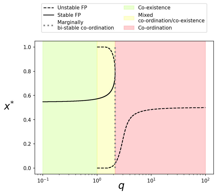
For the remainder of this section we focus on (we study the case in the SM, see for example Fig. S1). Figure 4 is analogous to Fig. 2, except now . What was previously a co-existence region for is now bi-stable co-ordination. What was /-dominance for is now classified as co-ordination so there is one large co-ordination region where the position of the interior fixed point varies continuously. The upper and lower boundaries between the mixed co-ordination/co-existence and co-ordination regions are where marginally bi-stable co-ordination occurs.
As we increase , the shapes of these regions change. We can choose particular values of and , and investigate how the fixed points move as is varied. This leads to a bifurcation diagram, as shown in Fig. 5. For and this particular choice of and we would have a co-existence type flow, the single interior fixed point is stable. For we move into a mixed co-ordination/co-existence regime, and two new interior fixed points spawn at the boundaries, both of which are unstable. As increases further the stable interior fixed point and one of the unstable interior fixed points move closer to one another, and meet at . Beyond this point, we find one interior fixed point, which is now unstable. This means that the flow is of the co-ordination type. The diagram confirms that small values of promote the minority strategy, i.e. if only a small fraction of individuals are of type , then will increase, and if only a small fraction of individuals are of type then will decrease. This produces a stable internal fixed point (co-existence). Conversely, large values of promote the majority strategy, leading to co-ordination type flows.
IV Fixation probability for a single invader, and fixation times
Having analysed the -deformed deterministic dynamics in infinite populations, we now look at the fixation probabilities and times in finite populations. We will focus on the Fermi update in Eq. (6). Our analysis follows the steps established for example in [30].
The fixation probability is the probability that the evolutionary process ends in a state in which the entire population is of type (as opposed to entirely of type ), if there are initially type individuals (and type individuals). The conditional average time to fixation is the expected time a single invader of type needs to take over a population consisting initially of individuals of type , given such a takeover happens. The unconditional average time to fixation is the expectation value of the time until the population is monomorphic ( or ) if there is initially one individual of type and individuals of type .
For the rates in Eq. (7), the probability is given by (see SM, Sec. S3.1)
| (14) |
Here, is defined as
| (15) |
where is the Pochhammer symbol [33]. The object is defined as
| (16) |
The fixation times can then be written (see SM, Sec. S3.2) as
| (17a) | ||||
| (17b) | ||||
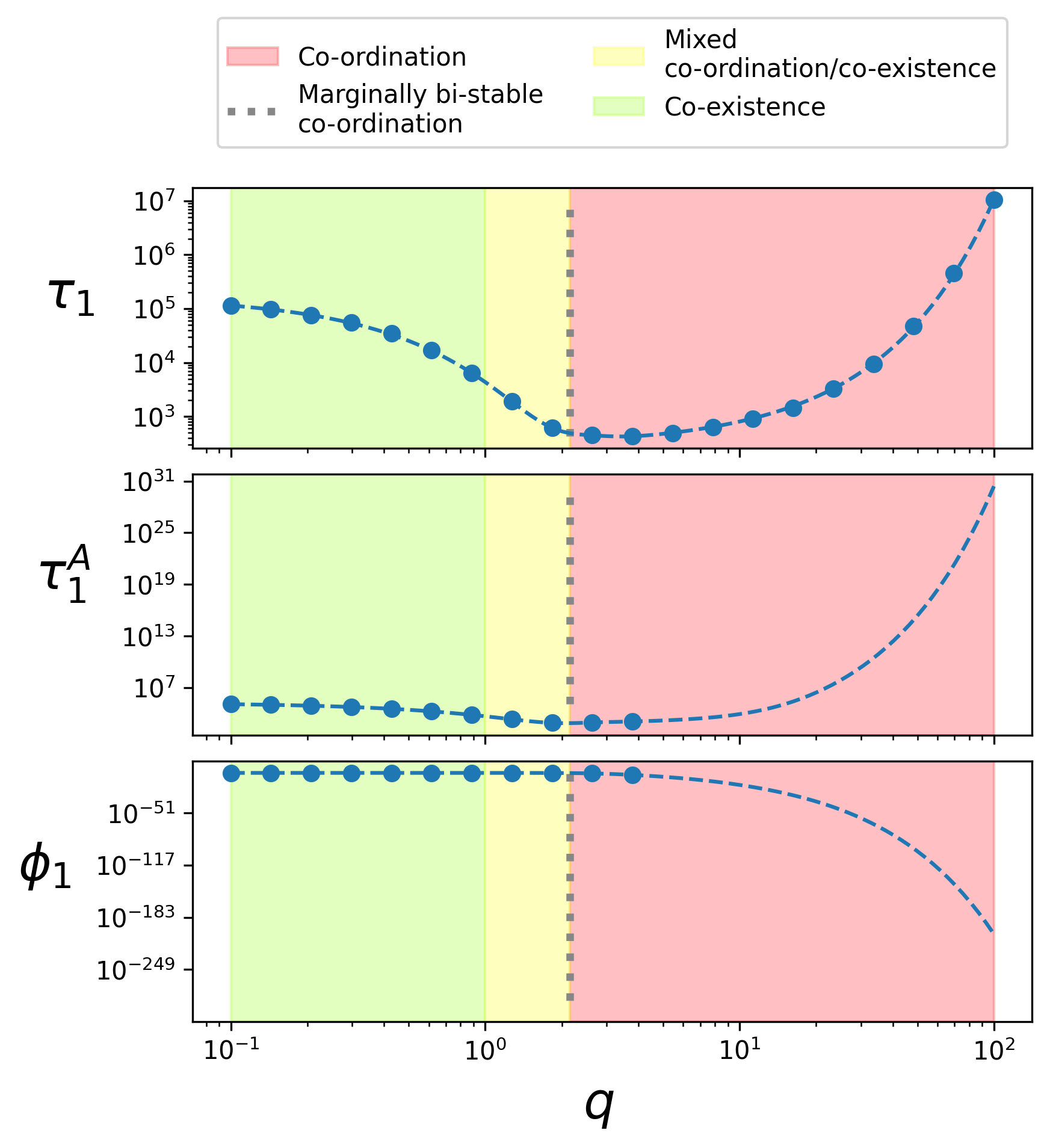
In Fig. 5 we showed how the interior fixed points, and hence the type of the evolutionary flow, change with for a fixed choice of and . In Fig. 6 we plot the unconditional and conditional fixation times [Eqs. (17a) and (17b)] as well as the fixation probability [Eq. (14)] as functions of , for the same game as in Fig. 5, and for a population of size .
For this particular system is of the co-existence type (green region in Figs. 5 and 6). Thus we expect trajectories of the stochastic dynamics for finite to move towards the co-existence fixed point, and then to remain near this meta-stable state until a large fluctuation drives the mutant to extinction or fixation. The escape time depends on the population size (the larger the population, the more difficult is the escape) and on the strength of the attraction of the fixed point. In the region the co-existence fixed points becomes less attractive as is increased (this is because for small , the deformation favours the minority strategy). This is in-line with the decrease of fixation times in Fig. 6. Consistent with this, the fixation probability decreases (from approximately to as changes from to ). This behaviour is not materially changed by the appearance of two additional unstable fixed points at (yellow region in Figs. 5 and 6).
For the deterministic system is of the co-ordination type (red region in Figs. 5 and 6). We then find that the evolutionary flow becomes smaller in absolute terms as is increased. This flow is given by the right-hand side of Eq. (8), and describes the net change of the system per unit time. For large actual events only occur very rarely in time, as changes in the population only happen when a sample of players all have the same type. Mathematically, the factors and become small when . Thus, the population dynamics becomes slower as is increased, in-line with the increase of the fixation times in the red region of Fig. 6.
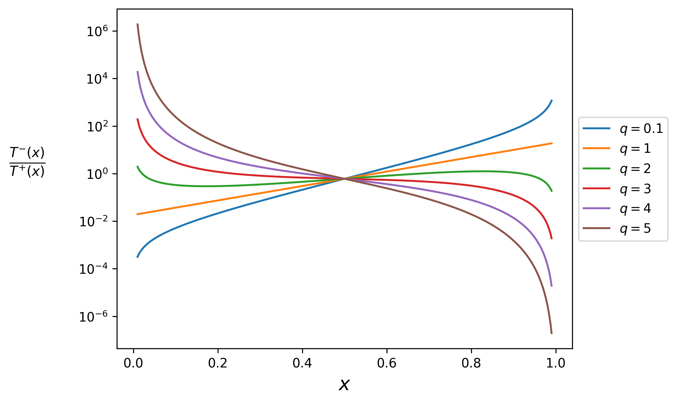
The fixation probability is not affected by time scales, but instead by the ratio of transition rates , as detailed in Eq. (S15) in the SM. Using Eqs. (6) and (7) we have
| (18) |
For large , the pre-factor dominates this expression. If is near zero the pre-factor is large, and thus, with overwhelming probability the next event in the population will lead to a decrease in mutant numbers. Similarly, when is near one, the pre-factor is small, and the next event in the population is very likely to lead to an increase of the number of mutants. In essence, -deformation favours the majority type for , and promotes co-ordination. As illustrated in Fig. S2 in the SM this effect becomes stronger as is increased. Thus, it becomes more difficult for a single mutant to take over the population, and decreases with in the co-ordination regime, as seen in the lower panel of Fig. 6.
V -deformed dynamics on graphs
So far we have only considered populations with all-to-all connectivity, i.e. the dynamics runs on a complete graph. We now extend the model to more general networks.
The dynamics on graphs are as follows. A random node is selected. In a second step random neighbours of that node are chosen at random with replacement. If all neighbours are in the opposite state to that of the node, it will change its state with a specific probability. This probability is as in Eq. (6), but the payoff difference that enters into the functions is now
| (19) |
Here is the number of type neighbours of the node chosen for potential update, and is its degree. The quantities and are as in Eq. (4). Thus, is the change in the expected payoff of the focal node if it switches from to .
Using the pair approximation we can derive differential equations that can be numerically integrated to approximately describe the density of type agents, , and the density of ‘active links’, , on infinite uncorrelated graphs (see SM, Sec. S4). A link in the network is said to be active when it connects two individuals of different types. These equations are of the form
| (20) | |||||
and
| (21) | |||||
Here is the degree distribution of the graph, and is the mean degree. The quantity is the probability that a type / node, which has degree , has neighbours of type . Under the pair approximation this is a binomial distribution (see SM, Sec. S4).
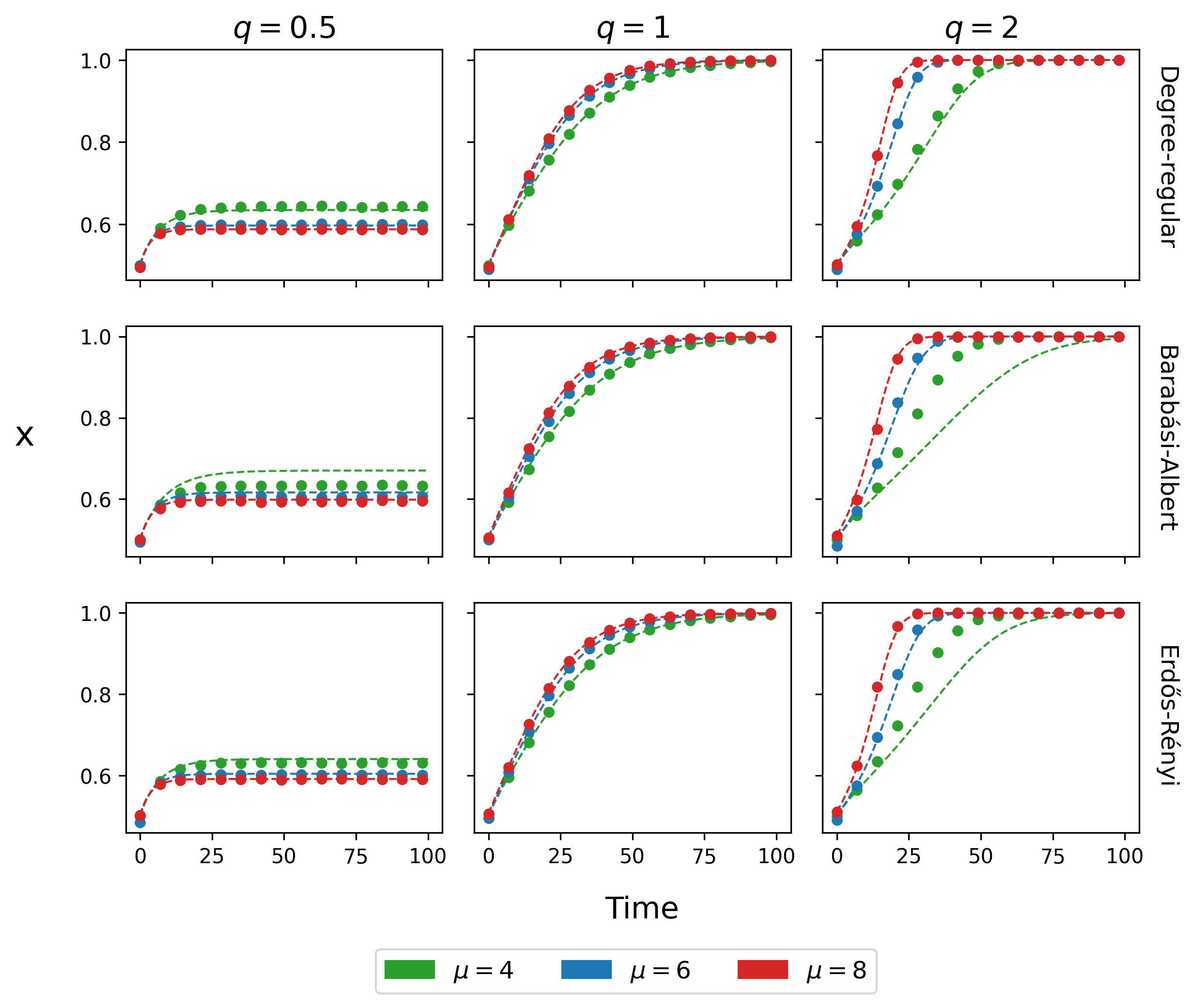
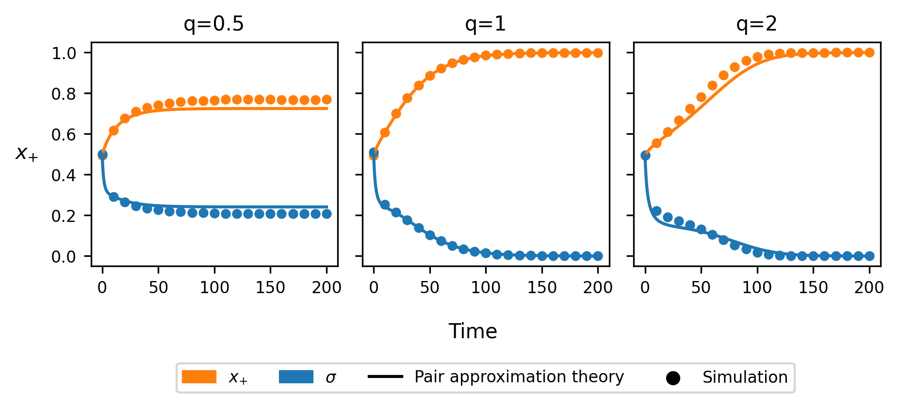
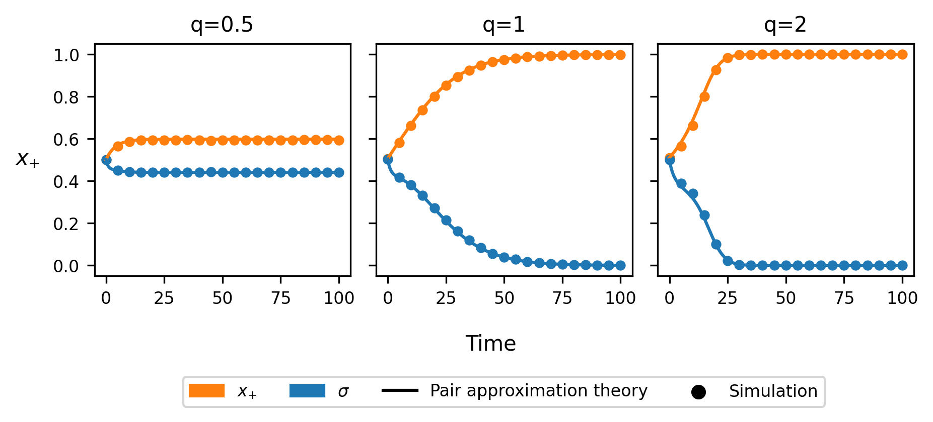
In Fig. 7 we show the average fraction of agents of type as a function of time for different graphs of varying average degree and for different values of . The upper three panels are for degree-regular graphs, and as the data shows the pair approximation captures simulation results well, even quantitatively. Deviations are seen for Barabási–Albert and Erdös–Reńyi graphs, in particular for (the largest value of shown in the figure). The pair approximation correctly predicts the convergence to , but the speed of the approach is underestimated, in particular for smaller mean degrees, where the pair approximation is known to breakdown [34].
Overall, Fig. 7 demonstrates that the structure of the network affects the dynamics. In the examples shown, the effects of the mean degree are limited to intermediate times for for all graphs we have tested. This is because in the long-run the system fixates , and the stability of this state is not affected in the range of mean degrees tested in Fig. 7. It is interesting to note that the dynamics in the pair-approximation can have multiple stable fixed points. We find this to be the case for (see Fig. S4 in the SM, indicating co-ordination-type behaviour). Convergence to is then only seen for some initial conditions.
The long-term average density of type agents itself is affected for (left-hand panels in Fig. 7). We note that the stationary density is here strictly between zero and one. Changes of the mean degree then directly alter the location of this fixed point of Eqs. (20) and (21).
The main purpose of this section was to describe how the pair approximation can be extended to -deformed game dynamics. We stress again that the focal agent in our setup compares its current expected payoff to that it would receive if it were to change strategy. This is at variance with some existing studies of game dynamics on networks, where interaction only occurs with one single neighbour () [35]. If there is only one interaction partner, it is perhaps natural to compare the payoffs of the focal node and that of the interaction partner. However, for , the focal node interacts with multiple other agents, so that payoff comparison with one single neighbour does not seem sensible. As an alternative to our dynamics one could consider a model in which the focal agent compares its current payoff to the average payoff of neighbours (but again changes can only occur provided these neighbours are all of the same type). While we expect that the pair approximation can be developed also in such a scenario, we have not pursued this here. The main reason is that the resulting theory would become more cumbersome, as the evaluation of the functions is then no longer local, but would also have to be based on the payoffs of the neighbours of the focal node, which in turn will depend on the degrees of those neighbours, and the states of the neighbours of the neighbours.
VI Multi-strategy cyclic games
VI.1 -deformed dynamics for multi-strategy games
We now consider games with strategies, writing for the payoff that an agent playing strategy receives when playing against an agent using strategy . We also write for the proportion of individuals in the population playing strategy , and introduce the column vector , where stands for transpose. We have . The average payoff of strategy is then
| (22) |
We focus on populations with all-to-all interactions. The individual-based process is as before. We choose one individual at random for potential update, say this individual is of type . In a second step individuals are sampled from the population (with replacement). Only if all of these individuals are of the same type (which we will call ) can a change of the original type individual occur. If this is the case, the update from to is implemented with probability .
The rate for changes from to is then
| (23) |
where we use the Fermi function and define, similar to Eq. (6),
| (24) |
As in Sec. III we use these rates to obtain equations which govern the dynamics of the average density of type agents in infinite populations. We find
| (25) |
In the case of two strategies, we recover Eq. (8).
VI.2 Three-strategy cyclic games
As an example we consider cyclic games with three pure strategies. This generalises the well-known rock-paper-scissors (RPS) game. Following [36, 37] we use the payoff matrix
| (26) |
where is real-valued. There are then two main model parameters, and . Our notation follows that of [36], we note that a different parametrisation is used for example in [37]. In the SM (Sec. S5) we also analyse a more general two-parameter family of payoff matrices.
We focus mostly on the case , such that the payoff to strategy ‘scissors’ for example is positive when playing against ‘paper’. Each pure strategy then beats one other pure strategy, and is beaten by the remaining pure strategy. The case can also be analysed, but the game is then not a bona fide cyclic game.
The centre of the strategy simplex is a fixed point of the dynamics for all and , indicating co-existence of all three strategies. The monomorphic states at the corners are also fixed points (only one type of strategy survives). Performing a linear stability analysis (see SM, Sec. S5) we find that the co-existence fixed point is linearly stable if and only if
| (27) |
The eigenvalues are complex for all , and thus the fixed point is a spiral sink for , and a spiral source for . When the fixed point is a centre.
A linear stability analysis of the corners show that these are stable (with two real-valued eigenvalues) for . For the leading order-terms in the rate equations are sub-linear near the corners, and linear stability analysis does not apply. Nonetheless, the corners can be seen to be sources. When the corners are saddle points for all . Section S5 in the SM contains further details.
For the above payoff matrix is known to show different dynamics depending on the value of [37, 36]. For trajectories spiral to the centre of the strategy simplex, i.e. the densities of all strategies tend to . When we have neutrally stable cyclic orbits around the central fixed point. For one finds heteroclinc cycles, where the trajectories orbit near the edge of the simplex. For completeness we remark that the corners of the strategy simplex are stable fixed points when and . One then finds convergence to the corners.
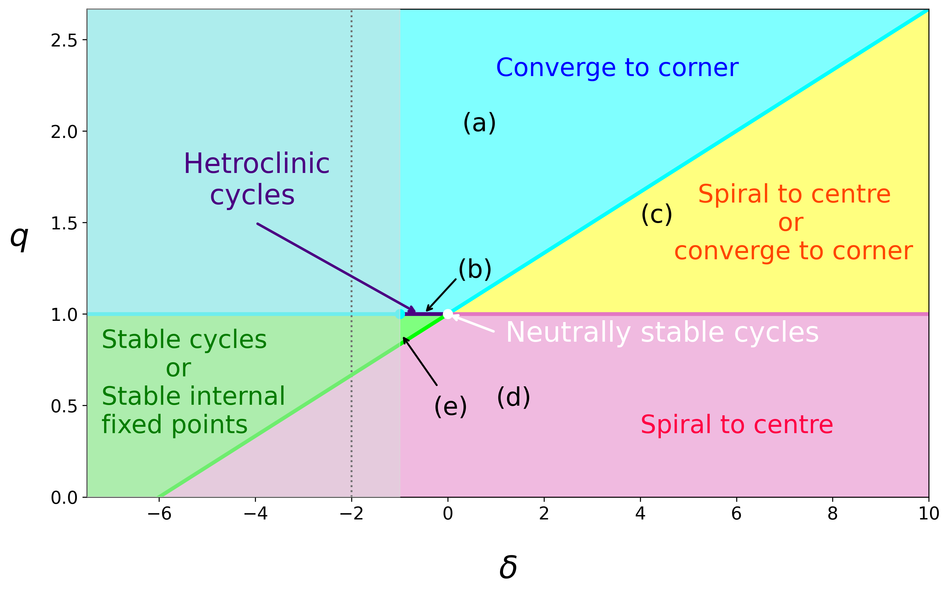
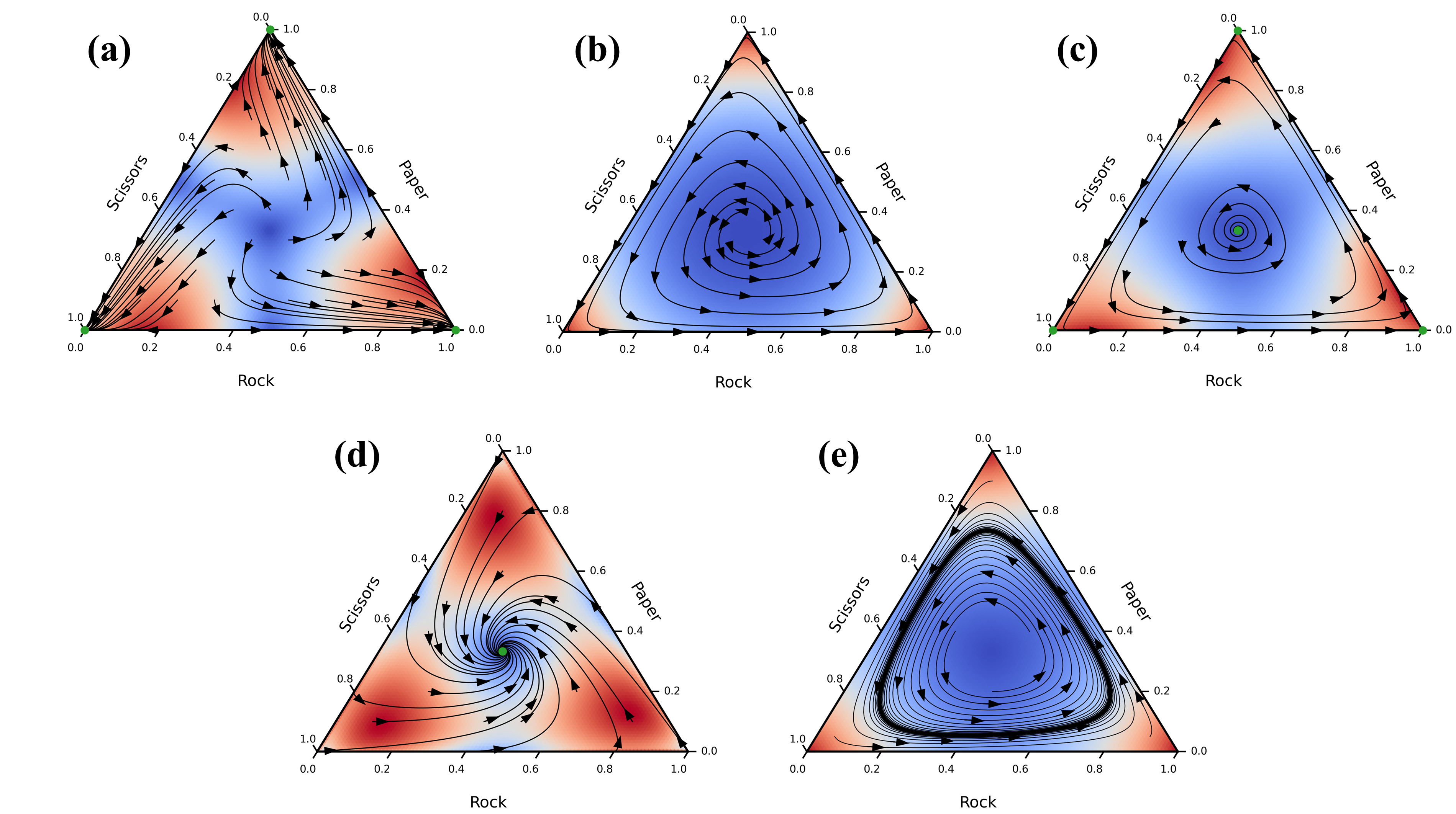
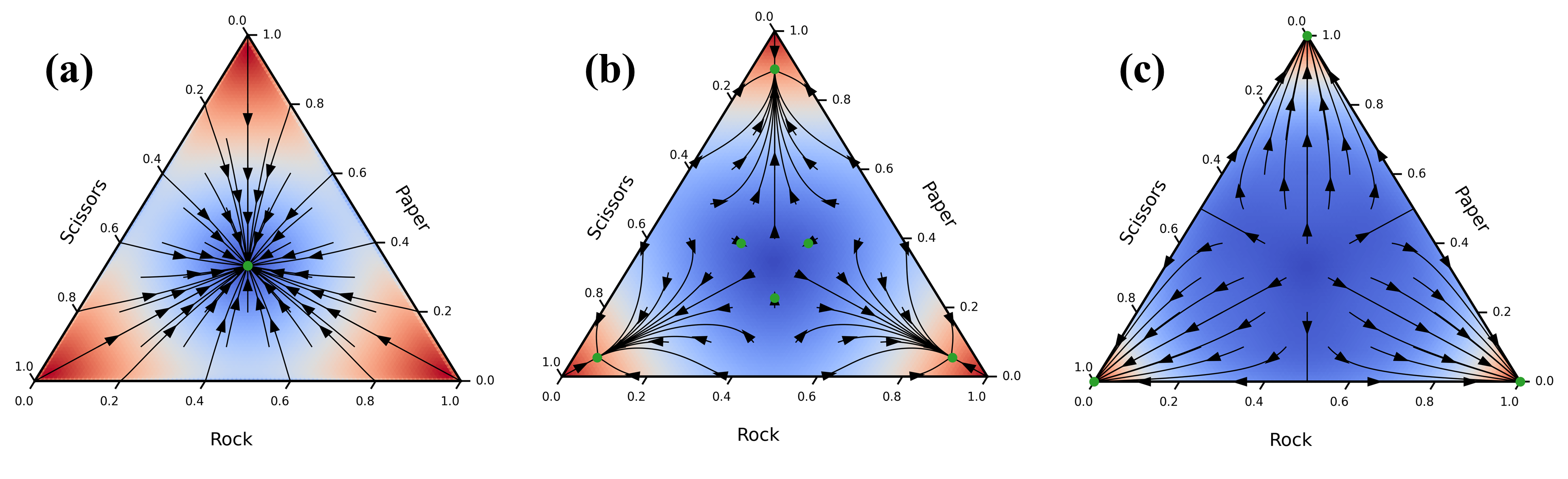
In Fig. 8 we show a phase diagram in the -plane highlighting the different types of outcome for the cyclic 3-strategy game for different and . We emphasise that the behaviour in the different phases is determined from the stability analysis of the corners and the centre, combined with numerical exploration of the -deformed rate equations. We cannot exclude the possibility of further fixed points in the interior, or on the edges of the simplex (see also SM, Sec. S5.4). Subject to this disclaimer, we find that -deformation can generate new types of flow, which we will now describe in turn.
When and (yellow region in Fig. 8) the dynamics either spirals to the centre or converges to one of the corners, depending on initial conditions. For , with , or with , (cyan region, including the cyan lines) we find convergence to one of the corners, which corner depends again on initial conditions. For and (green region, including the green line), we either have stable limit cycles or trajectories converge to stable internal fixed points that are not the centre or the corners. The latter tends to occur for , an example is given in SM, Sec. S5.4. In the indigo region () the system shows heteroclinic cycles. For (white point in the diagram) one finds neutrally stable cycles. Finally for , or with , (pink region, including the pink line) the dynamics spirals to the centre. For completeness we have included some range of in Fig. 8, even if the payoff matrix there does not describe a bona fide cyclic game. is a special case where the centre is a stable/unstable star (see SM, Sec. S5.4).
In Fig. 9 we illustrate these different types of flow in the strategy simplex. The choice for are as annotated in Fig. 8.
VII -deformed dynamics without replacement
Until now we have always assumed that the neighbours of the focal agent are chosen with replacement (i.e. the same individual can be chosen more than once). In this section, we focus on the case without replacement. It now only makes sense to consider integer values of . We focus on 2-strategy 2-player games and populations with all-to-all interaction. The state of the population is then fully described by the number of individuals playing strategy .
The rates for the events in the model without replacement are
| (28a) | ||||
| (28b) | ||||
respectively, where we have defined . We have for , this is because there must be at least type agents in the system in order for a type agent to select type other agents without replacement. Similarly for . More detail on these rates can be found in Sec. S6 of the SM.
Given the rates in Eqs. (28a) and (28b) we derive the fixation probability to be (see again Sec. S6 in the SM):
| (29) |
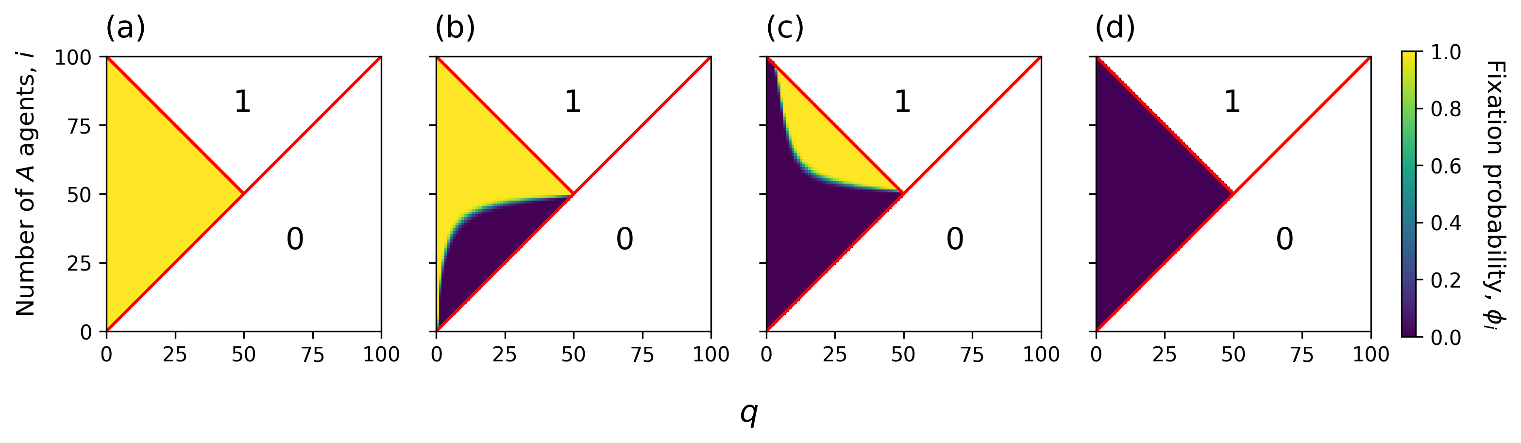
Here with as in Eqs. (28a) and (28b). The fixation probabilities are better illustrated in ()-space, as shown in Fig. 10 for different choices of and . The interesting region is that defined by the middle condition of Eq. (29) as this is the only region where the fixation probability depends on the game (in the other two regions, the fixation probability is zero or one respectively, independent of and ). We highlight this in Fig. 10, the region of interest is that in the triangle on the left of each panel.
In Fig. 10(a) the fixation probability is very close to one in this area. Since and are large in panel (a) this would typically be an -dominance game (see Fig. 2). At the other extreme ( and sufficiently negative) the flow is mostly of the -dominance type [Fig. 10(d)], and in the region of interest the fixation probability is very close to zero. For intermediate values of and the region of interest divides non-trivially into two areas, one in which is close to one, and another in which the fixation probability is close to zero [panels (b) and (c)].
VIII Discussion
In summary, we have combined ideas from the non-linear -voter model with dynamics in evolutionary game theory. The -voter model was originally introduced as a non-linear extension of the conventional voter model, and with a view towards understanding how non-linearity affects the statistical physics of simple systems with absorbing states. Evolutionary game dynamics is non-linear by itself, thus the goal of this work was to study how additional -deformation affects the outcome both in infinite and in finite populations. For integer there is a clear interpretation of the dynamics: an agent in the population consults with other agents. If all those other agents are in a state which is different from that of the focal agent, that latter agent considers a change of strategy. This is then implemented with a probability based on payoff gain. Mathematically, the model can be studied for any real-valued .
As we have seen, the combination of -deformation and selection because of the underlying game can produce a number of new types of flow, not seen in conventional game dynamics (). In games multiple internal fixed points become possible, thus generating scenarios such as bi-stable co-existence or mixed co-existence and co-ordination. We have systematically studied where in the space of games these different cases occur, as is varied. In cyclic games with three strategies one also finds dynamics which are not possible without -deformation, notably stable limit cycles and deterministic flow converging to pure-strategy points. We also find cases with multiple attracting fixed points in the interior of the strategy simplex (Sec. S5.4). Finally, we have shown how fixation times and probabilities can be calculated for -deformed dynamics in finite populations, and we have extended pair approximation methods for interacting agents on networks to -deformed processes.
The main purpose of this paper is to introduce the general idea of -deformation in game dynamics, to study a number of basic scenarios and to put the relevant tools in place. There are a number of lines which could be pursued in future work. For example, it might be interesting to see how -deformation affects the ordering dynamics of evolutionary games on regular lattices. One might expect departures from the universality class of directed percolation for example [35]. Similarly, one could study more systematically how the system departs from the -voter model in the limit of weak selection.
More generally, changing the strength of selection in an evolving population can have surprising effects. For example, so-called ‘stochastic slowdown’ has been reported [38], that is the conditional fixation time of a mutant can decrease even if the selective advantage of the mutant is increased. Non-monotonic behaviour of the conditional fixation time as a function of selection strength has also been observed [39]. Our analysis has shown that -deformation also affects fixation times. It would be interesting to investigate if effects similar to stochastic slowdown also occur. We note that -deformation not only changes the strength of evolutionary flow but also the location of co-existence fixed points. This is not the case in [38, 39], where the position of fixed points remain the same as the strength of selection is changed.
Acknowledgements
This work was supported by the the Agencia Estatal de Investigación and Fondo Europeo de Desarrollo Regional (FEDER, UE) under project APASOS (PID2021-122256NB-C21, PID2021-122256NB-C22), the María de Maeztu programme for Units of Excellence, CEX2021-001164-M funded by MCIN/AEI/10.13039/501100011033. We also acknowledge a studentship by the Engineering and Physical Sciences Research Council (EPSRC, UK), reference EP/T517823/1.
—— Supplemental Material ——
S1 Deriving the -deformed rate equations
We focus on a well-mixed population of size , and a game with two pure strategies. Define as the probability for the system to be in state at time , where is the number of type individuals. Given that the dynamics can be described via the rates and , which increase/decrease by respectively, the master equation can be written
| (S1) |
From this, the first moment , which is the average density of type agents, has the following differential equation,
| (S2) |
Assuming the population is of infinite size, we can ignore fluctuations. This means that the probability distribution , i.e. the solution to the master equation in Eq. (S1), is concentrated on its mean,
| (S3) |
With this we can simplify the average rates that appear in Eq. (S2),
| (S4) |
We ease the notation by writing as just , thus we have
| (S5) |
We can then use the rates from Eq. (7) to get the ‘-deformed’ dynamics in Eq. (8).
S2 Classifying -deformed evolutionary dynamics
To classify the outcome of -deformed dynamics for games we determine all fixed points, , and their stability.
S2.1 Fixed points and stability
The fixed points are obtained by setting the right-hand side of Eq. (8) to zero,
| (S6) |
Of course are trivial solutions corresponding to fixed points on the boundaries. We will determine their stability below. To find the interior fixed points we define
| (S7) |
assuming . The solutions to would give all interior fixed points. However, this is a non-linear equation with no analytic solution in general. Despite this, it is still possible to determine the dynamics for some given function .
We assume that takes the form of the Fermi function, as in Eq. (6). Equation (S7) then becomes
| (S8) |
This function only exists in the interval . We find
| (S9a) | ||||
| (S9b) | ||||
Since is a continuous function there must therefore be at least one zero, so there is always at least one interior fixed point. The maximum number of zeroes is determined by the number of stationary points (extrema) of , alongside the signs of at those stationary points. For example, if there are two stationary points and if takes a positive value at one of these point, and a negative value at the other, then has three zeroes, and hence there are three interior fixed points.
Differentiating Eq. (S8) and equating to zero gives the quadratic equation
| (S10) |
which has solutions
| (S11) |
These are the locations of the stationary points of the function in Eq. (S8). Thus, depending on the values of the parameters and , we can have zero, one or two stationary points.
The possible scenarios are as follows:
-
(i)
, has no stationary points. Thus has one zero, meaning there is one interior fixed point.
-
(ii)
, has one stationary point at , so has one zero, and there is one interior fixed point.
-
(iii)
, has two stationary points, and , both of which are in the interval . This leads to the following sub-scenarios:
-
(a)
The two stationary points have opposite signs, i.e. , which means has three zeroes, hence there are three interior fixed points.
-
(b)
The two stationary points have the same sign, i.e. , which means has one zero, and hence there is one interior fixed point.
-
(c)
One stationary point lies exactly on the axis , i.e. either or , which means crosses the horizontal axis once and touches it once at another location. Hence, there are two interior fixed points.
-
(a)
-
(iv)
, Eq. (S11) has two solutions but they lie outside of the range . Since is bounded on these are not valid solutions. Thus has no stationary points, which means it crosses the -axis once, so one interior fixed point.
Next we determine the stability of the boundary fixed points. If , then and will always be both greater than zero or both less than zero. For one will be greater than zero and the other less than zero. This can be easily proved by first assuming [Eq. (S6)]. Then manipulate the inequality into the form of Eq. (S8), at which point we find (if ) or (if ), i.e. the same/opposite sign to .
Now, we know from Eq. (S9a) that is negative as , thus for , will also be negative in this limit. This means that the fixed point at is stable. We can use a similar argument to show that the fixed point at is also stable.
The stability of the interior fixed points can be determined in the same way. For example, if and have the same sign, and only crosses the horizontal axis [] once, there is one interior fixed point, and that fixed point must be unstable.
The above classifications are summarised in Tab. S1. Graphical representations of these classifications are shown in Fig. 3. We note that there are four scenarios that lead to ‘marginally bi-stable’ flow. These types of flow are rare in comparison to the others. We group the classifications into two pairs: ‘marginally bi-stable co-existence’ and ‘marginally bi-stable co-ordination’. The difference within a pair is the ordering of the two interior fixed points.
| Discriminant classification | Stationary point value | value of | Classification |
| or | N/A | Co-ordination | |
| Co-existence | |||
| Co-ordination | |||
| Co-existence | |||
| Mixed co-ordination/co-existence | |||
| Bi-stable co-existence | |||
| Marginally bi-stable co-ordination | |||
| Marginally bi-stable co-existence | |||
| Marginally bi-stable co-ordination | |||
| Marginally bi-stable co-existence |
S2.2 Phase diagram
S2.2.1 General analysis
These classifications are better illustrated by a phase plot in the -plane, which will also help to highlight how the -deformed flow changes as we alter the payoff matrix. We first want to determine all points in the -plane that would give marginally bi-stable flow. To do this we substitute the stationary point solutions and , given by Eq. (S11), into [Eq. (S8)], then set this equal to zero and solve. This is equivalent to solving which, as seen from Tab. S1, is what defines marginally bi-stable flow. We find
| (S12a) | ||||
| (S12b) | ||||
Recall from Eq. (S11) that are functions of and , thus for a given value of , Eqs. (S12a) and (S12b) are lines in the -plane. These equations are only valid for when , and for when , where
| (S13) |
Otherwise Eq. (S11) does not have real solutions.
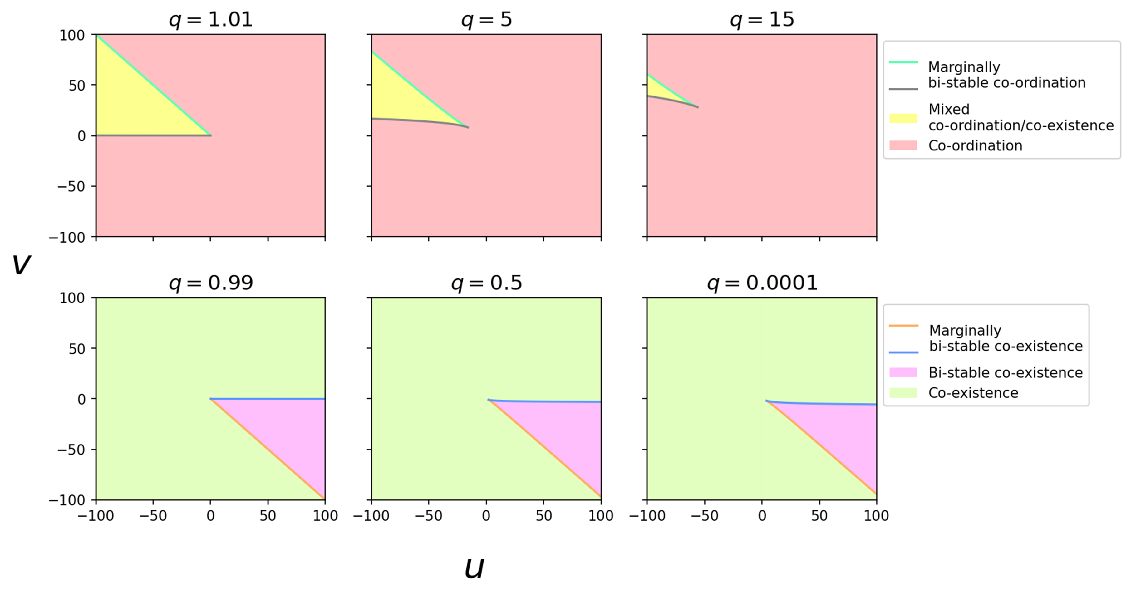
Along the line defined by one has , i.e. marginally bi-stable co-ordination and marginally bi-stable co-existence for and respectively. Similarly, sitting on the line corresponds to , again marginally bi-stable co-ordination and marginally bi-stable co-existence for and respectively. The region between these lines corresponds to , i.e. mixed co-ordination/co-existence or bi-stable co-existence for and respectively. The region outside of these lines is simply standard co-ordination or co-existence for and respectively.
Fig. S1 demonstrates the idea for different values of . This figure highlights the fact that marginally bi-stable co-ordination and marginally bi-stable co-existence type flow are rare, as they are only seen on well defined lines in the -plane. Most of the time we see either co-ordination/co-existence, or mixed co-ordination/co-existence () and bi-stable co-existence ().
S2.2.2 The limit
In the limit both and go to zero for any . Thus Eq. (S6) is satisfied for all values of , meaning all such points are fixed points. This is because for no events can occur in a population containing individuals both of type and type .
S2.2.3 Large, but finite
For large but finite , the mixed co-ordination/co-existence region shrinks and standard co-ordination dominates due to the fact that becomes large and negative [see Eq. (S13)], which is the upper bound for for the mixed co-ordination/co-existence region. The interior fixed point of the dominating co-ordination region is at all points in the space classified as co-ordination. This can be seen by noting that as becomes large
| (S14) |
and has one solution, namely . So for large positive we only get co-ordination type flow with , and we conclude that dynamics promotes the majority, i.e. if there are less types than types the dynamics drives the population of types down to zero.
Since is only large, but still finite, there always exists a region of mixed co-ordination/co-existence (yellow region in Fig. S1), but only for large negative , and . This is because in the standard case these mixed co-ordination/co-existence regions are co-existence regions [see Fig. 2]. The dynamics promotes the minority, i.e. if there are less types the dynamics attempts to drive the number upwards. In this way, there is a balance between the the game itself favouring the minority, and the -deformation for promoting the majority. As we increase , the influence of the -deformation dominates, and the mixed co-ordination/co-existence region shrinks.
S2.2.4 The limit
In the limit , the -deformation favours co-existence. This time however, is a finite limit [see Eq. (S13)]. Thus there always exists a region of bi-stable co-existence (even for ), as seen in the lower panels of Fig. S1. The reasoning for this is analogous to that for large finite : the -deformed dynamics promotes the minority while the standard replicator flow () in this region would promote the majority [see Fig. 2]. Decreasing initially means the influence of the -deformation increases, so co-existence starts to take over. However, past a certain point this effect diminishes, and decreasing further results in no change.
S3 Fixation probability and fixation time for games with -deformed dynamics
S3.1 Fixation probability
For an initial number of type agents, , we want to calculate the fixation probability , which is the probability for the system to reach the state , i.e. all agents in the population are of type .
It is well known that [10]
| (S15) |
where . Using the transition rates for our model, Eq. (7), we can write
| (S16) |
We note that . Using the Fermi function as the choice for [Eq. (6)], we can write the ratio
| (S17) |
Thus we have
| (S18) |
which can be interpreted as the tendency for the system to decrease the number of type agents. Again, we define , where is as in Eq. (3).
We now follow the lines of [30]. Equation (S15) requires evaluating the product
| (S19) |
where is the Pochhammer symbol [33] and we have used the formula for the payoff difference as in Eq. (3). The summation inside the exponential has a simple closed form which we will write as
| (S20) |
We also define the following function which appears in Eq. (S19) as
| (S21) |
With this we can write the fixation probability as
| (S22) |
In the limit , we recover the known formula for the standard Fermi process (with no deformation) [30, p; 5].
S3.2 Fixation time
We want to calculate the unconditional, , and conditional, , fixation times for -deformed dynamics. is the time it would take type agents to take over the population, whereas is the time it would take for the type agents to take over or become extinct, both starting from a single type agent.
For general event rates of the one-step process these can be calculated as [10]
| (S23a) | ||||
| (S23b) | ||||
where is the ratio of transition probabilities, given by Eq. (S18), and is the probability to fixate from type agents, given by Eq. (14). These equations can be written in a simpler form by evaluating the product, analogous to what was done in Sec. S3.1,
| (S24) |
Thus the fixation times can be written,
| (S25a) | ||||
| (S25b) | ||||
where and are the functions defined in Eqs. (15) and (16) respectively.
S3.3 Further results for the system in Figs. 5 and 6
Further results for the system in Figs. 5 and 6 can be found in Fig. S2. For the flow is of the co-ordination type. The figure shows that increasing in this regime makes it more and more likely that the next event is towards the absorbing monomorphic states at and . This reduces the probability for a single mutant to take over the population.
S4 Pair approximation on graphs
S4.1 Notation
We now analyse -deformed dynamics on graphs. We assign each node a state if it is an or type respectively. We focus on undirected graphs.
We perform a homogeneous pair approximation, similar to [41, 42]. This approximation is known to capture the behaviour of the model to good accuracy on infinite uncorrelated graphs [43]. By uncorrelated graphs we mean graphs where nodes have no preference for attaching to nodes of any particular degree [44].
We write the degree distribution of a general graph as . This is the probability that a randomly chosen node in the graph has degree (i.e. neighbours). We denote the number of type neighbours of a node as . A node in state and of degree with type neighbours will often be referred to as an node.
S4.2 Rate of change of the proportion of agents of type
We wish to determine a differential equation for , which we define to be the average density of nodes in the +1 state. By average we mean average over independent realisations of the dynamics. The angle-bracket notation is dropped to ease notation and keep consistency with the rest of the paper and the literature. We assume a time step of , and take in order to obtain the continuous-time limit, thus the following now only applies to infinite graphs.
The general rate equation for is
| (S26) |
where is the rate at which nodes flip to nodes, and is the amount changes when this happens. The factor in the denominator results from a division by the time-step.
It can be seen by inspection that , therefore
| (S27) |
S4.3 The homogeneous pair approximation
Determining the rates will require knowing the probability that a node in state with degree has neighbours in the state , we will denote this probability . To derive an expression for we will use the homogeneous pair approximation. This assumes that the states of the different neighbours are independent, and leads to a binomial distribution of the form
| (S28) |
where is the single-event probability that a node in state is connected to a node in state +1. This probability can be defined in terms of the density of state- nodes, , and a quantity which is the density of links connecting opposite spin nodes. We refer to as the density of active interfaces/links, in-line with standard voter model terminology [41]. The conditional probability can be determined as follows: is the ratio of the number of links connecting opposite-state nodes to the total number of state nodes,
| (S29) |
The probability can then be easily determined from
| (S30) |
Thus, combining Eqs. (S29) and (S30) we have the general expression
| (S31) |
The moments of can then be evaluated. As we will see below, only the first and second moments are needed, which are and respectively, where is shorthand for from Eq. (S31).
We emphasise that we have assumed that the probability of selecting a link connecting nodes in opposite states, , is independent of the degree of the nodes which it connects. This is a shortcoming of the homogeneous pair approximation. Extensions have been proposed, such as the heterogeneous pair approximation [34], which allows to depend on degree. Similarly, we assume an infinite graph. The stochastic pair approximation [45] accounts for finite-size corrections. However, here, we do not consider these extensions.
S4.4 Rate of change of
Due to the presence of in the binomial moments, the differential equations for will be coupled to the differential equation for . The general form for such an equation has an analogous form to Eq. (S26),
| (S32) |
Again is the rate at which nodes flip to nodes. The quantity is the corresponding change in the density of active links. Assuming it is an node that flips to a node, for there are active links initially, and active links after flipping, thus a change of . There are links overall, so the change in the density of active links is . Similar analysis for gives overall . Therefore we can write Eq. (S32) as
| (S33) |
S4.5 Transition rates on graphs
The dynamics we have considered so far on complete graphs is a form of pairwise comparison dynamics. A node is chosen at random, of its neighbours are then chosen. If all neighbours are of opposite type to the originally selected node, the node will change type with a probability given by the Fermi function [Eq. (6)]. The argument of this function is the payoff difference , i.e. the difference in the average payoff of the node and one of its neighbours. This is fine to do, as on a complete graph all neighbours have the same payoff (if they are all in the same state).
On general graphs things are different. A node will select random neighbours, but, even if they are all in the same state, those neighbours do not necessarily have the same average payoff, as they themselves have different neighbourhoods. Instead then on a general graph we replace where
| (S34) |
Here is the average payoff of an node, it is defined analogously to Eq. (2). then is the increment in the average payoff when an node changes to an node. In other words, decisions are based on comparing the payoff to one node with the payoff this node would receive if it changed state (and keeping all neighbours in their present state). We thus introduce [Eq. (6)]
| (S35) |
This gives the probability that an node changes to an node. When , the average payoff of the node being spin is much larger than it being spin , accordingly, meaning the node is guaranteed to flip.
We can now form expressions for which are needed for Eqs. (S27) and (S33). We have
| (S36a) | ||||
| (S36b) | ||||
Consider Eq. (S36a), which is the rate at which the density of nodes increase under our modified pairwise comparison dynamics. For this to happen an node must be picked at random, this gives rise to the first three terms. random neighbours in the state must then picked, which happens with probability . The node must then decide to switch its state with probability . Eq. (S36b) has an analogous structure where an node becomes and node.
S4.6 Analytically tractable limits
We will now evaluate Eqs. (S37a) and (S37b) in some analytically tractable limits to check their validity. These are the voter model (Sec. S4.6.1) and the complete graph (Sec. S4.6.2)
S4.6.1 Voter model limit
The limit , (since we absorbed into and this means having ) is the standard voter model and Eqs. (S37a) and (S37b) should reproduce known results from [41].
Eq. (S37a) becomes
| (S38) |
where is the first moment of the binomial distribution defined in Eq. (S28). So the average density of nodes in state +1 does not change with time as expected in the standard voter model.
Eq. (S37b) becomes
| (S39) |
where is the second moment of the binomial distribution defined in Eq. (S28). With the replacement , and moving to the steady-state we find
| (S40) |
where is the long-term stationary fraction of agents of type . The pre-factor describes the long-lived plateau of the density of active links reported in [41].
S4.6.2 Complete graph limit
The degree distribution of a complete graph is a delta function peaked around , i.e. . Furthermore, the binomial distributions defined in Eq. (S28) are also delta functions peaked around , i.e. . This is because every node is connected and there are nodes in state +1, so the probability any node has neighbours is 1, and 0 for any other number of +1 neighbours.
S4.7 Degree-regular graphs
For degree-regular graphs Eqs. (S37a) and (S37b) simplify significantly. The degree distribution is simply a delta function peaked at , i.e. , which collapses the outer summations over , so we have
| (S43a) | |||
| (S43b) | |||
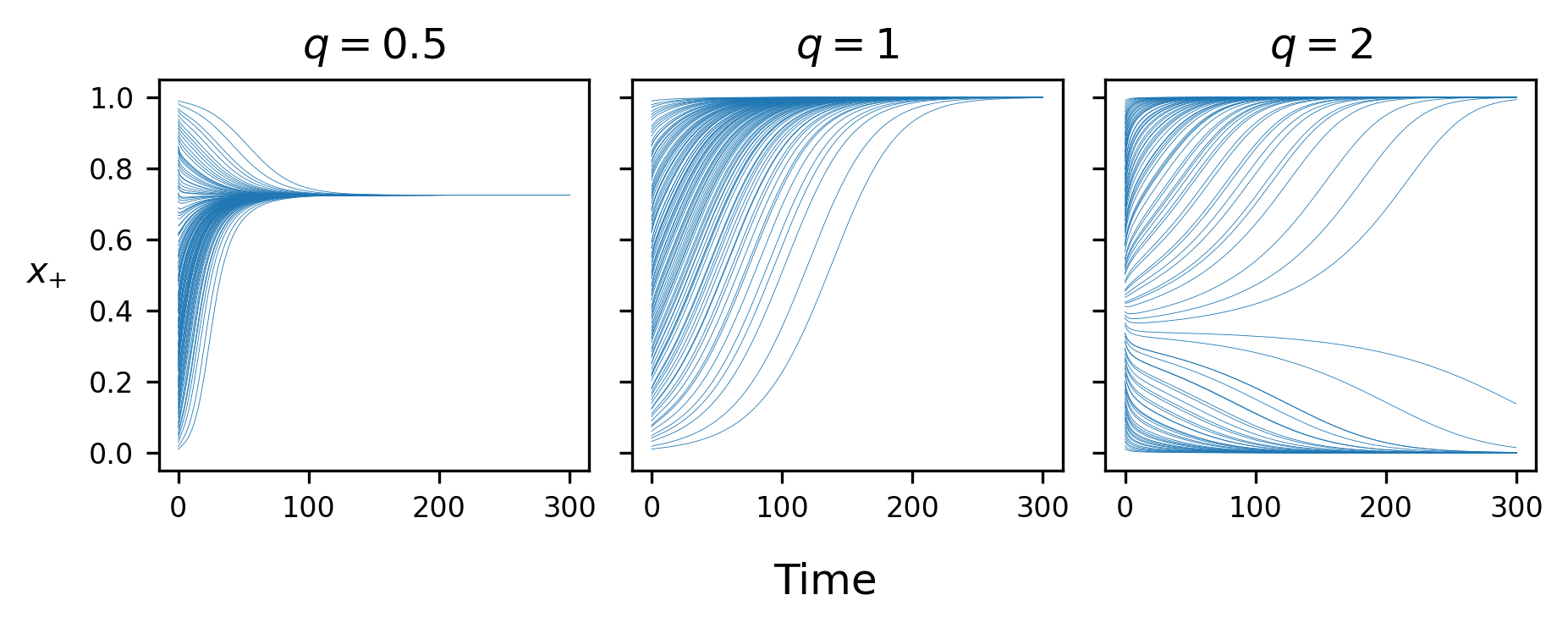
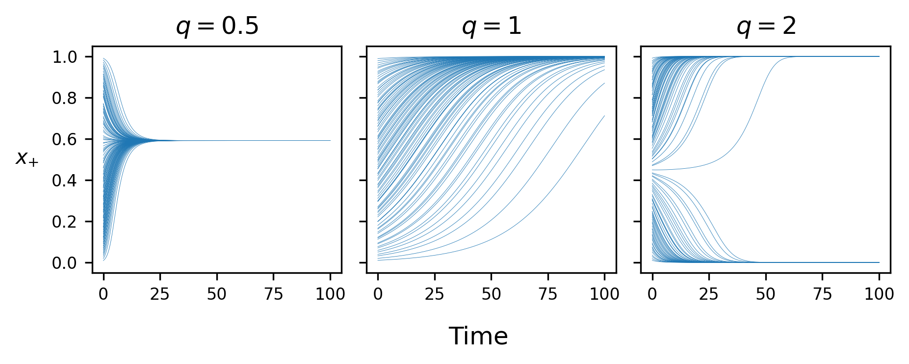
This pair of coupled differential equations can be numerically integrated and in Fig. S3 we show some example trajectories for a single degree-regular graph, varying the parameter . The approximation works fairly well given the coarse nature of the pair approximation.
To classify the dynamics for a given set of parameters we can look at multiple pair approximation trajectories for different initial densities of type nodes, this is shown in Fig. S4. For there is a stable fixed point at around , thus the flow could be classified as co-existence type. This is in-line with the idea that small values of promote the minority, as discussed for complete graphs in Sec. S2. For (standard game dynamics) there is a stable fixed point at , which is unsurprising as the parameters chosen correspond to an -dominance type flow for complete graphs [see Sec. S2]. For there appears to be an unstable fixed point just below , thus this flow could be classified as co-ordination type. Again this is in line with Sec. S2 where we found large values of promote the majority.
S4.8 Non-regular graphs
The case of graphs which are not regular is more difficult. We use Eqs. (S37a) and (S37b) but we have to perform the summation over the degree distribution .
We show in Figs. S5 and S6 analogous plots to Figs. S3 and S4 but now for Barabási–Albert and Erdös–Rényi graphs respectively to demonstrate the validity of the solution for different heterogeneous uncorrelated (or approximately uncorrelated) graphs.
We note that in Fig. S5 the analytical results agree very well with simulation, even more than for degree-regular graphs (Fig. S3). This is likely because in Fig. S3 whereas in Fig. S5 . This form of pair approximation is known to breakdown at lower [34].
S5 -deformed dynamics for cyclic games
We wish to determine the classification of the -deformed dynamics for cyclic games [such as the rock-paper-scissors (RPS) game]. In this appendix we study games defined by the payoff matrix
| (S44) |
This is a generalisation of Eq. (26). We study the dynamics for general and .
The centre of the strategy simplex is always a fixed point, as are the pure strategies at the corners of the simplex. We thus study the linear stability of these fixed points. We note that there are only two degrees of freedom in the system since .
An accompanying Mathematica notebook with further details of the following calculations can be found at a GitHub repository [46].
S5.1 The centre point
Here we analyse the stability of the point . The Jacobian of the dynamics in Eq. (25) (after reduction to two degrees of freedom) evaluated at the centre is
| (S45) |
The eigenvalues of this matrix are,
| (S46) |
Assuming , both eigenvalues are complex, and thus the point can only be a centre, spiral sink, or spiral source [47]. For centres, we require the real part of the eigenvalues to be zero, this occurs when
| (S47) |
When , the real part of both eigenvalues is negative, so will be a spiral sink. When , the real part of both eigenvalues is positive, so will be a spiral source.
In the special case of , we have a single real eigenvalue with algebraic multiplicity 2,
| (S48) |
The eigenspace has geometric multiplicity 2, i.e. there are two linearly independent eigenvectors corresponding to this eigenvalue, namely and . This means that is a star, which is a source when , i.e. , and a sink when , i.e. . When we have a centre once again.
For general and then, is some form of sink when , some form of source when , and a centre when .
S5.2 The corners
Here we analyse the stability of the corners, , i.e. permutations of the point . By symmetry all corners give the same results from stability analysis.
S5.2.1
When the eigenvalues of are
| (S49a) | |||
| (S49b) | |||
Thus both eigenvalues are real. If both , then the corners are sources. If both , then the corners are sinks. If and have opposite signs then the corners are saddle points.
For all entries in the payoff matrix are zero. There is thus no actual game dynamics, and the flow is solely determined by the -deformation. For the case (no deformation), which we are discussing here, this means that there is no dynamics at all ( for all ).
S5.2.2
When the eigenvalues of are
| (S50a) | |||
| (S50b) | |||
Thus for all both eigenvalues are real and negative, hence the corners are always sinks.
S5.2.3
For any the rate equations are (after reduction to two degrees of freedom, which we will call and , these are the proportions of two of the strategies):
| (S51a) | ||||
| (S51b) | ||||
The right-hand sides evaluate to zero at the corners of the strategy simplex (, , and respectively). Due to the symmetry with respect to interchange of types, it is sufficient to study the stability of the fixed point at one of the three corners, here we choose . For and small, but non-zero, and keeping in mind that we focus on , the leading order terms on the right are proportional to or . Therefore, linear stability analysis cannot be used. When both and are small, Eqs. (S51a) and (S51b) reduce to
| (S52a) | ||||
| (S52b) | ||||
Therefore, both for small (but positive). This is the case for all and , so the corners are always sources.
S5.3 Reduction to one-parameter family of payoff matrices
We have shown in Sec. S5.2 that the stability of the corners is independent of and , except when where only the signs of and matter. In Sec. S5.1 we showed that determines the stability of the centre.
In principle our analysis allows for a complete classification of the flows (as far as linear stability analysis goes) for all values of and .
In order to reduce the number of parameters we now fix and focus on positive values of . This reflects the scenario of a cyclic game. Each strategy is beaten by one other strategy, and in turns beats the remaining strategy. It is convenient to set (following [36]). In this way reflects the standard zero-sum rock-paper-scissors game. The constraint translates into . We note that other (equivalent) setups have been used, see for example [37]. For this reduced setup Eq. (S47) becomes
| (S53) |
The centre fixed point is a stable spiral for and an unstable spiral for . It is a centre for .
The corners are sources for and sinks for , as this is independent of . For the corners are saddle points for all , otherwise they are sinks.
S5.4 Further ternary plots
As mentioned in Sec. S5.1, when (or in the reduced setup ) the centre point is a stable or unstable star depending on the value of .
For the centre point is a stable star. As shown in Sec. S5.2 the corners in this region are sources. This leads to trajectories moving directly towards the centre point as illustrated in Fig. S7(a)
For the centre point is now an unstable star. Again the corners in this region are sources. This leads to stable fixed points that are inside the simplex as illustrated by the green markers in Fig. S7(b). We note that stable internal fixed points could arise anywhere in the green region in Fig. 8, not just for . However, when moves further from the centre becomes a stronger spiral sink/source, which forces trajectories into stable orbits rather than to stable fixed points.
For the centre point is still an unstable star but the corners becomes sinks. This leads to trajectories moving directly away from the centre point, converging at the corners as illustrated in Fig. S7(c).
S6 Fixation probability for -deformed dynamics without replacement for games
As in Sec. S3.1 we want to calculate the fixation probability , except now for an adapted version of the model where we select an integer number of neighbours without replacement.
The rates for the model without replacement are defined as follows:
| (S54a) | ||||
| (S54b) | ||||
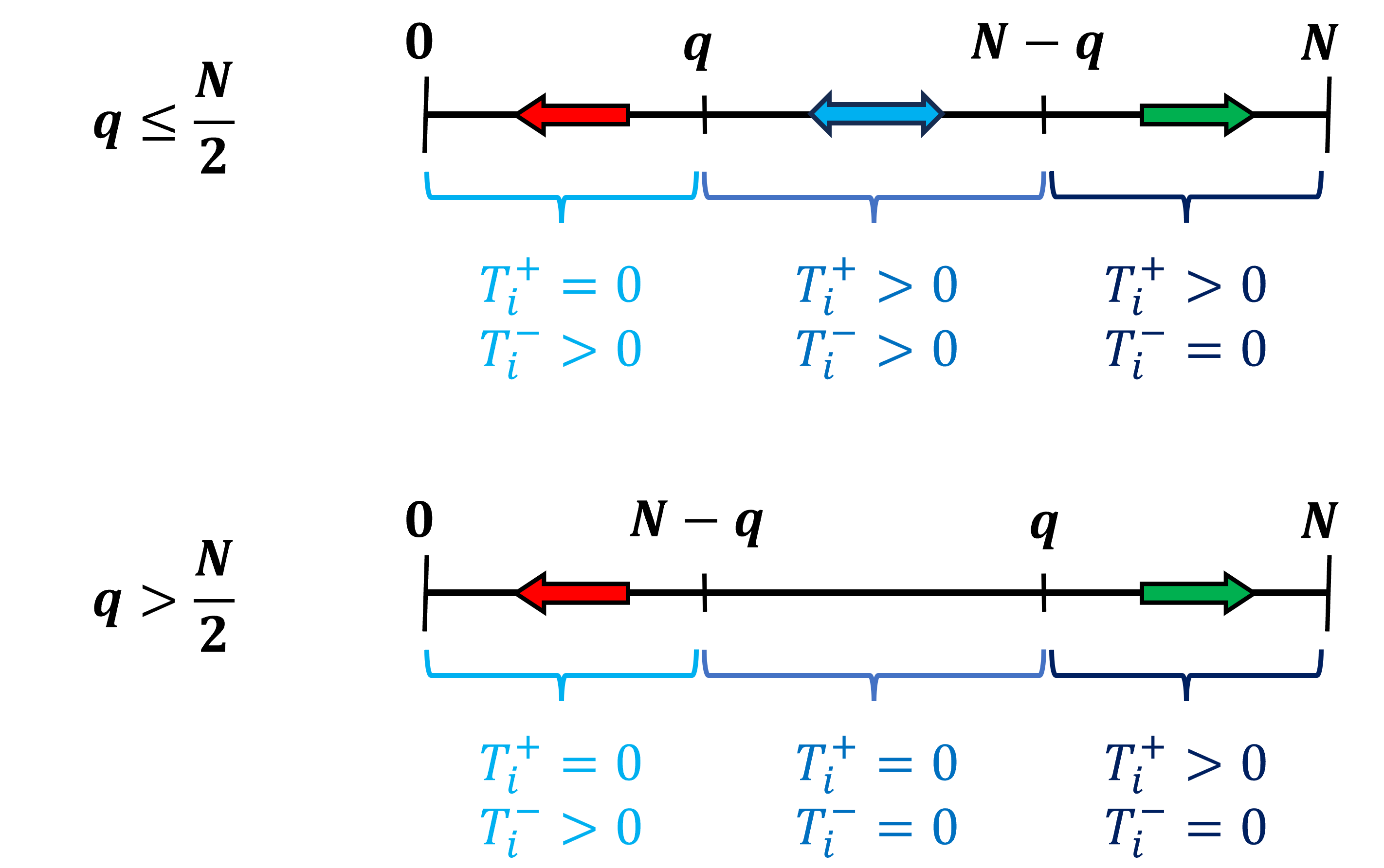
Fig. S8 illustrates the rates for the cases of and . We see that it is often the case that the system is driven to one of the absorbing states at or . For and both and are non-zero so the system can move in either direction. For and both and are 0 so the system does not move. This is because we require at least or agents in order for a node to choose neighbours of the opposite type.
For the case , the probability to fixate with all agents being type is trivially if and if . For we write the recursive expression
| (S55) |
Rearranging this equation, and defining , we find , where is the ratio of the transmission rates. Unlike in the model with replacement [Eq. (S18)], has a piecewise definition:
| (S56) |
Noting that is the smallest non-zero , we can write
| (S57) |
for . Now, assuming we can manipulate into the following form,
| (S58) |
noting the first line is possible as all values other than , which is zero anyway, cancel. In going from the third to fourth line we use Eq. (S57). To determine we use the largest that we know to be equal to one, i.e. ,
| (S59) |
Substituting Eq. (S59) into Eq. (S58) we get an expression for the fixation probability in the intermediate regime,
| (S60) |
When all cases are trivial. and give as or respectively as the system is forced to the absorbing states. The intermediate case of gives , as the system cannot move. Overall then for we have for , and for .
Combining all results we have for the fixation probability:
| (S61) |
References
- von Neumann [1928] John von Neumann. Zur theorie der gesellschaftsspiele. Mathematische annalen, 100(1):295–320, 1928.
- Von Neumann [1959] John Von Neumann. On the theory of games of strategy. Contributions to the Theory of Games, 4:13–42, 1959.
- Von Neumann and Morgenstern [2007] John Von Neumann and Oskar Morgenstern. Theory of games and economic behavior. In Theory of games and economic behavior. Princeton university press, 2007.
- Smith and Price [1973] John Maynard Smith and George R Price. The logic of animal conflict. Nature, 246(5427):15–18, 1973.
- Smith [1982] John Maynard Smith. Evolution and the Theory of Games. Cambridge university press, 1982.
- Gintis [2000] Herbert Gintis. Game theory evolving. Princeton University Press, Princeton, 2000.
- Hofbauer and Sigmund [2003] Josef Hofbauer and Karl Sigmund. Evolutionary game dynamics. Bulletin of the American mathematical society, 40(4):479–519, 2003.
- Taylor et al. [2004] Christine Taylor, Drew Fudenberg, Akira Sasaki, and Martin A. Nowak. Evolutionary game dynamics in finite populations. Bulletin of Mathematical Biology, 66(6):1621–1644, 2004.
- Traulsen et al. [2005] Arne Traulsen, Jens Christian Claussen, and Christoph Hauert. Coevolutionary dynamics: from finite to infinite populations. Physical review letters, 95(23):238701, 2005.
- Traulsen and Hauert [2009] Arne Traulsen and Christoph Hauert. Stochastic evolutionary game dynamics. Reviews of nonlinear dynamics and complexity, 2:25–61, 2009.
- Lieberman et al. [2005] Erez Lieberman, Christoph Hauert, and Martin A. Nowak. Evolutionary dynamics on graphs. Nature, 433:312–316, 2005.
- Traulsen et al. [2006a] Arne Traulsen, Jens Christian Claussen, and Christoph Hauert. Coevolutionary dynamics in large, but finite populations. Phys. Rev. E, 74:011901, 2006a.
- Claussen [2007] Jens Christian Claussen. Drift reversal in asymmetric coevolutionary conflicts: influence of microscopic processes and population size. Eur. Phys. J. B, 60:391–399, 2007.
- Bladon et al. [2010] Alex J Bladon, Tobias Galla, and Alan J McKane. Evolutionary dynamics, intrinsic noise, and cycles of cooperation. Phys. Rev. E, 81(6):066122, 2010.
- Traulsen et al. [2006b] Arne Traulsen, Martin A Nowak, and Jorge M Pacheco. Stochastic dynamics of invasion and fixation. Physical Review E, 74(1):011909, 2006b.
- Holley and Liggett [1975] Richard A Holley and Thomas M Liggett. Ergodic theorems for weakly interacting infinite systems and the voter model. The annals of probability, pages 643–663, 1975.
- Granovsky and Madras [1995] Boris L Granovsky and Neal Madras. The noisy voter model. Stochastic Processes and their applications, 55(1):23–43, 1995.
- Mobilia et al. [2007] Mauro Mobilia, Anna Petersen, and Sidney Redner. On the role of zealotry in the voter model. Journal of Statistical Mechanics: Theory and Experiment, 2007(08):P08029, 2007.
- Masuda [2013] Naoki Masuda. Voter models with contrarian agents. Physical Review E—Statistical, Nonlinear, and Soft Matter Physics, 88(5):052803, 2013.
- Castellano et al. [2009a] Claudio Castellano, Santo Fortunato, and Vittorio Loreto. Statistical physics of social dynamics. Reviews of modern physics, 81(2):591–646, 2009a.
- Redner [2019] Sidney Redner. Reality-inspired voter models: A mini-review. Comptes Rendus Physique, 20(4):275–292, 2019.
- Castellano et al. [2009b] Claudio Castellano, Miguel A Muñoz, and Romualdo Pastor-Satorras. Nonlinear q-voter model. Physical Review E, 80(4):041129, 2009b.
- Mobilia [2015] Mauro Mobilia. Nonlinear -voter model with inflexible zealots. Phys. Rev. E, 92:012803, 2015.
- Ramirez et al. [2024] Lucía S. Ramirez, Federico Vazquez, Maxi San Miguel, and Tobias Galla. Ordering dynamics of nonlinear voter models. Phys. Rev. E, 109:034307, 2024.
- Blume [1993] Lawrence E Blume. The statistical mechanics of strategic interaction. Games and economic behavior, 5(3):387–424, 1993.
- Timpanaro and Prado [2014] André M Timpanaro and Carmen PC Prado. Exit probability of the one-dimensional q-voter model: Analytical results and simulations for large networks. Physical Review E, 89(5):052808, 2014.
- Mellor et al. [2016] Andrew Mellor, Mauro Mobilia, and RKP Zia. Characterization of the nonequilibrium steady state of a heterogeneous nonlinear q-voter model with zealotry. Europhysics Letters, 113(4):48001, 2016.
- Jedrzejewski [2017] Arkadiusz Jedrzejewski. Pair approximation for the q-voter model with independence on complex networks. Physical Review E, 95(1):012307, 2017.
- Nyczka et al. [2012] Piotr Nyczka, Katarzyna Sznajd-Weron, and Jerzy Cisło. Phase transitions in the q-voter model with two types of stochastic driving. Physical Review E—Statistical, Nonlinear, and Soft Matter Physics, 86(1):011105, 2012.
- Altrock and Traulsen [2009] Philipp M Altrock and Arne Traulsen. Fixation times in evolutionary games under weak selection. New Journal of Physics, 11(1):013012, 2009.
- sup [2024] The supplement contains further details of the model and the theoretical and numerical analysis (url to be inserted by copy editor), 2024.
- Nowak [2006] Martin A Nowak. Evolutionary dynamics: exploring the equations of life. Harvard university press, 2006.
- Abramowitz and Stegun [1948] Milton Abramowitz and Irene A Stegun. Handbook of mathematical functions with formulas, graphs, and mathematical tables, volume 55. US Government printing office, 1948.
- Pugliese and Castellano [2009] Emanuele Pugliese and Claudio Castellano. Heterogeneous pair approximation for voter models on networks. Europhysics Letters, 88(5):58004, 2009.
- Szabó and Fáth [2007] György Szabó and Gábor Fáth. Evolutionary games on graphs. Physics Reports, 446(4):97–216, 2007.
- Yu et al. [2016] Qian Yu, Debin Fang, Xiaoling Zhang, Chen Jin, and Qiyu Ren. Stochastic evolution dynamic of the rock–scissors–paper game based on a quasi birth and death process. Scientific reports, 6(1):28585, 2016.
- Mobilia [2010] Mauro Mobilia. Oscillatory dynamics in rock–paper–scissors games with mutations. Journal of Theoretical Biology, 264(1):1–10, 2010. ISSN 0022-5193.
- Altrock et al. [2010] Philipp M. Altrock, Chaitanya S. Gokhale, and Arne Traulsen. Stochastic slowdown in evolutionary processes. Phys. Rev. E, 82:011925, 2010.
- Altrock et al. [2012] Philipp M. Altrock, Arne Traulsen, and Tobias Galla. The mechanics of stochastic slowdown in evolutionary games. Journal of Theoretical Biology, 311:94–106, 2012.
- Hindersin and Traulsen [2015] Laura Hindersin and Arne Traulsen. Most undirected random graphs are amplifiers of selection for birth-death dynamics, but suppressors of selection for death-birth dynamics. PLOS Computational Biology, 11(11):1–14, 11 2015.
- Vazquez and Eguíluz [2008] Federico Vazquez and Víctor M Eguíluz. Analytical solution of the voter model on uncorrelated networks. New Journal of Physics, 10(6):063011, 2008.
- Kitching et al. [2024] Christopher R Kitching, Henri Kauhanen, Jordan Abbott, Deepthi Gopal, Ricardo Bermúdez-Otero, and Tobias Galla. Estimating transmission noise on networks from stationary local order. arXiv preprint arXiv:2405.12023, 2024.
- Gleeson [2013] James P Gleeson. Binary-state dynamics on complex networks: Pair approximation and beyond. Physical Review X, 3(2):021004, 2013.
- Dorogovtsev [2010] Sergey Dorogovtsev. Lectures on Complex Networks. Oxford University Press, 02 2010.
- Peralta et al. [2018] Antonio F Peralta, Adrián Carro, M San Miguel, and Raúl Toral. Stochastic pair approximation treatment of the noisy voter model. New Journal of Physics, 20(10):103045, 2018.
- R. Kitching [2024] Christopher R. Kitching. q-deformed evolutionary dynamics in simple matrix games, May 2024. URL https://github.com/C-Kitching/q-deformed-evolutionary-dynamics-in-simple-matrix-games.
- Strogatz [2018] Steven H Strogatz. Nonlinear dynamics and chaos with student solutions manual: With applications to physics, biology, chemistry, and engineering. CRC press, 2018.