EM++: A parameter learning framework for stochastic switching systems

Abstract

This paper proposes a general switching dynamical system model, and a custom majorization-minimization-based algorithm EM++ for identifying its parameters. For certain families of distributions, such as Gaussian distributions, this algorithm reduces to the well-known expectation-maximization method. We prove global convergence of the algorithm under suitable assumptions, thus addressing an important open issue in the switching system identification literature. The effectiveness of both the proposed model and algorithm is validated through extensive numerical experiments.

, , ,

[cor]Corresponding author. Tel: +32 16 32 03 64

1 Introduction

Obtaining a realistic model is of crucial importance in any model-based control application. Yet, as the complexity of the underlying systems keeps on increasing, deriving such models from first principles becomes ever more difficult. This evolution has motivated the development of data-driven modelling methods. Black-box models like neural networks can capture complex dynamics, but are challenging to analyze. By contrast, switching systems approximate complicated nonlinear systems as a combination of simple systems, and as such offer a good balance between simplicity and expressiveness [38, 36].

Switching dynamical systems are dynamical systems which consist of a set of subsystems, and some switching mechanism that governs which of these subsystems is active at a given time. The switching mechanism may be either subsystem-state-dependent, or -independent [36]. A state-dependent switching mechanism often utilizes polyhedral partitioning, in which case the activation of a subsystem depends on whether a regressor vector lies within a given region, either deterministically [15, 18, 8] or probabilistically [25, 31]. On the other hand, Markov jump systems are popular examples of state-independent switching systems. The switching probability of these models is determined by a fixed transition matrix [17, 23, 21]. Moreover, [9, 32] propose general frameworks covering both types of switching mechanisms, which iteratively identify the subsystem parameters and the most probable subsystem combination weights for each data point. However, during inference these models repeatedly solve an optimization problem to determine the weights for each predicted data point, potentially limiting their integration with optimization-based controllers.

Although it is convenient to model subsystems as linear systems with additive Gaussian noise [23, 28, 10], this choice may not always be suitable for the data at hand. For instance, hidden Markov models [40] typically involve observations from categorical distributions. The exponential family [49, 19] is a general distribution class that includes both Gaussian and categorical distributions, making it more versatile for modelling diverse types of data. However, a limitation of the exponential family is its inability to capture many commonly occurring heavy-tailed distributions [27, 1]. Such distributions offer an alternative option for modelling subsystems, and provide more robustness against outliers [33, 21].

Algorithms for identifying switching systems are typically optimization-based [36], and consist of two primary variants: coordinate-descent methods [8, 32, 9, 10] and expectation-maximization methods [23, 21, 28, 45]. Despite achieving good experimental performance, most methods lack convergence guarantees. We remark that some optimality guarantees for coordinate-descent-based methods have been provided [8, 32], but these do not ensure convergence to stationary points.

In this work, we present an identification method for generalized switching systems based on the majorization-minimization (MM) principle [22, 30]. This principle includes the EM algorithm as a special case. The subsequential convergence of MM schemes has been proven under generic conditions [30, §. 7.3] [41]. However, verifying whether these hold is usually only straightforward when the involved functions are smooth. In such smooth case, [29] connects the EM algorithm with the mirror descent algorithm [6, 13], which is similar to a classical gradient descent method, but replaces the Euclidean distance term by a so-called Bregman distance [14]. In a similar way, the (subsequential) convergence of the EM algorithm has been analyzed in [47, 16, 29] by interpreting EM as a non-Euclidean descent method. However, these works focus on identifying a static model with i.i.d. data. For a more general problem setup, [51, 46] also prove sequential convergence of related methods, but under a discrete set assumption that may be difficult to verify.

Our contributions can be summarized as follows.

1. We present a general switching system model that generalizes the one proposed in [28] to more generic subsystem dynamics. The model includes: 1 A parametric formulation for the switching mechanism that can be either subsystem-state-dependent or -independent. In contrast to [9, 32], this parametric formulation only requires the evaluation of the identified model during inference. 2 A generic subsystem dynamics formulation covering various popular distributions, including the exponential family, as well as a number of heavy-tailed distributions.

2. We introduce an MM-based identification algorithm EM++ for the proposed model and establish its global subsequential convergence to stationary points, even when the probability densities include nonsmooth functions. Our method generalizes the EM method to identify a significantly wider class of switching systems. Additionally, we extend the convergence analysis of the EM algorithm beyond the canonical exponential family and i.i.d. data presented in [29]. We prove full sequence convergence to a stationary point under a mild Kurdyka-Łojasiewicz (KL) condition [34], which improves upon existing results even in the EM setting.

3. We confirm the expressiveness of the proposed model and the effectiveness of the identification method through a series of numerical experiments.

Overview. Section 2 introduces a general switching system and the corresponding identification problem. Section 3 presents the proposed method for solving this problem, and Section 4 analyzes its convergence. Section 5 details how to effectively evaluate the key functions in the problem. Section 6 experimentally shows the efficiency of both the model and algorithm.

Notation. Denote the cone of $m\times m$ positive definite matrices by $\mathbb{S}_{++}^{m}$. Let $\left\lVert A\right\rVert^{2}_{B}\!{}\mathop{\mathrel{:}=}{}\!\operatorname{tr}(A^{\top}BA)$ for $B\in\mathbb{S}_{++}^{m}$. Let $\mathrm{I\!N}_{[a,b]}\!=\!\mathrm{I\!N}\cap[a,b]$ and $\mathbf{1}_{d}\!=\!\begin{bmatrix}1&\dots&1\end{bmatrix}\in\mathrm{I\!R}^{d}$. Define $\mathrm{lse}:\mathrm{I\!R}^{d}\to\mathrm{I\!R}$ as $\mathrm{lse}(x)\!=\!\ln\big{(}\textstyle{\sum_{j=1}^{d}}\exp(x_{j})\big{)},$ and the softmax function $x\mapsto\sigma(x)$ with $\sigma_{i}(x)\!=\!\exp\big{(}x_{i}\big{)}/\sum_{j=1}^{d}\exp\big{(}x_{j}\big{)}$ the $i$th entry of the output $\sigma(x)$. Denote the class of $n$-times continuously differentiable functions by $\mathcal{C}^{n}$. Given a function $f$: $\mathcal{O}\subseteq\mathrm{I\!R}^{n}\to\mathrm{I\!R}$, we use the convention $\forall x\not\in\mathcal{O}$: $f(x)=+\infty$, and follow the definition of strict continuity of [43, Definition 9.1], which is equivalent to local Lipschitz-continuity. The directional derivative of $f$ at $x\in\mathcal{O}$ along $d\in\mathrm{I\!R}^{n}$ is defined as $f^{\prime}(x\operatorname{;}v)=\lim_{\lambda\searrow 0}\frac{f(x+\lambda v)-f(x)}{\lambda}.$ A function $f\in\mathcal{C}^{1}$ is Lipschitz smooth if $f$ has Lipschitz continuous gradients.

2 Problem statement

Table 1: List of pdf and pmf $p(y\mid z,\xi=j\operatorname{;}\bm{\beta})$ satisfying (1b). The first block are members of canonical exponential family [49, 19].

	Notation	$\beta_{j}$	C	$f(x)$	$\ell(y,z,\beta_{j})$	$g(y,z,\beta_{j})$
Exp. familya	$\quad\quad/$	$\beta$	$\eta(y,z)$	$x$	$-\langle\beta,\mathcal{T}(y,z)\rangle$	$\mathcal{A}(z,\beta)$
Categorical	$\mathrm{\mathsf{Cat}}(\sigma(\Theta^{\top}z))$	$\Theta$	1	$x$	$-\Theta_{y}^{\top}z$	$\mathrm{lse}(\Theta^{\top}z)$
Gaussian	$\mathcal{N}(\mu\!=\!Lz,\Sigma)$	$\begin{aligned} B=&\Lambda L\\[-3.0pt] \Lambda=&\Sigma^{-1}\end{aligned}$	$(2\pi)^{-n_{y}/2}$	$x$	$\frac{1}{2}\!\langle\Lambda,yy^{\top}\!\rangle{-}\langle B,zy^{\top}\!\rangle$	$\frac{1}{2}\!\big{(}\!\left\lVert Bz\right\rVert^{2}_{\Lambda^{{-}1}}\!{-}\ln\!\det(\!\Lambda\!)\!\big{)}$
Student’s tb [44]	$\mathrm{\mathsf{St}}_{\nu}(\mu=Lz,\Sigma)$	$\begin{aligned} B=&\Lambda L\\[-3.0pt] \Lambda=&\Sigma^{-1}\end{aligned}$	$\tfrac{\Gamma((\nu+n_{y})/2)}{\sqrt{(\pi\nu)^{n_{y}}}\Gamma(\nu/2)}$	$\frac{\nu{+}n_{y}}{2}\!\ln(\!1\!+\!\frac{2x}{\nu}\!)$	$\frac{1}{2}\left\lVert\Lambda y-Bz\right\rVert^{2}_{\Lambda^{-1}}$	$-\frac{1}{2}\ln\det(\Lambda)$
$\ell_{1}$-Laplace [2]	$\mathrm{\mathsf{Laplace}}(\mu\!=\!Lz,\!\Sigma)$	$\begin{aligned} M=&RL\\[-3.0pt] R=&\Sigma^{-\nicefrac{{1}}{{2}}}\end{aligned}$	$2^{-n_{y}/2}$	$\sqrt{2}x$	$\left\lVert Ry-Mz\right\rVert_{1}$	$-\sum_{i=1}^{n_{y}}\ln(R_{ii})$
Logistic [24, §23]	$\mathrm{\mathsf{Logistic}}(\mu\!=\!az,\!\varsigma)$	$\begin{aligned} b=&\lambda a\\[-3.0pt] \lambda=&\varsigma^{-1}\end{aligned}$	$\frac{1}{4}$	$2\ln(x)$	$\mathrm{cosh}(\frac{1}{2}(\lambda y-bz))$	$-\ln\lambda$
Gumbel [24, §22]	$\mathrm{\mathsf{Gumbel}}(\mu\!=\!az,\!\varsigma)$	$\begin{aligned} b=&\lambda a\\[-3.0pt] \lambda=&\varsigma^{-1}\end{aligned}$	$1$	$x$	$\exp(-\lambda y+bz)$	$-\ln\lambda+\lambda y-bz$

• Functions $\eta:\mathrm{I\!R}^{n_{y}}\times\mathrm{I\!R}^{n_{z}}\rightarrow\mathrm{I\!R}_{++}$, $\mathcal{T}:\mathrm{I\!R}^{n_{y}}\times\mathrm{I\!R}^{n_{z}}\rightarrow\mathcal{B}$, $\mathcal{A}:\mathrm{I\!R}^{n_{z}}\times\mathcal{X}_{\beta}\rightarrow\mathrm{I\!R}$.

• With given degrees of freedom $\nu$.

We consider a stochastic dynamical system that switches among $d$ linear subsystems, and is characterized by

$$\xi_{t+1}\!\sim \,p(\xi_{t+1}\mid z_{t},\xi_{t}=i\operatorname{;}\bm{\Theta})=\sigma_{\xi_{t+1}}\big{(}\Theta_{i}^{\top}z_{t}\big{)},$$ (1a)

$$y_{t+1}\!\sim \,p(y_{t+1}\mid z_{t},\xi_{t+1}=j\operatorname{;}\bm{\beta})$$

$$= \,C\!\exp\!\big{(}{-}f(\ell(y_{t+1},z_{t},\beta_{j}))\!-\!g(y_{t+1},z_{t},\beta_{j})\big{)}{,}$$ (1b)

where at time $t\geq 0$ the random variables $\xi_{t}\in\Xi=\{1,\dots,d\}$ and $y_{t}\in\mathrm{I\!R}^{n_{y}}$ are the active subsystem index and the observation, respectively. Both $\xi_{t}$ and $y_{t}$ depend on the trajectory history

$$z_{t}=\Upsilon(y_{t},\dots,y_{t-t_{y}+1})$$ (2)

where $\Upsilon:\mathrm{I\!R}^{t_{y}n_{y}}\rightarrow\mathrm{I\!R}^{n_{z}}$ is a known (non-)linear mapping with the window length $t_{y}>0$. The switching mechanism (1a) is modelled with a softmax function composed with a mapping that is linear w.r.t the parameter $\bm{\Theta}{}\mathop{\mathrel{:}=}{}\{\Theta_{i}\}_{i=1}^{d}$ with $\Theta_{i}\in\mathrm{I\!R}^{n_{z}\times d}$. With $\bm{\beta}{}\mathop{\mathrel{:}=}{}\{\beta_{i}\}_{i=1}^{d}\in\mathcal{B}^{d}$ where $\mathcal{B}$ is a Euclidean parameter space, the subsystem dynamics (1b) is modelled by a distribution with a probability density function (pdf) or probability mass function (pmf) defined by a parameter-invariant term $C>0$ and functions $f$, $\ell$, and $g$ under the following assumption.

Assumption 2.1 (Subsystem model).

Regarding the functions in (1b), i.e., $f:\mathcal{X}_{f}\rightarrow\mathrm{I\!R}$, $\ell:\mathrm{I\!R}^{n_{y}}\times\mathrm{I\!R}^{n_{z}}\times\mathcal{X}_{\beta}\rightarrow\mathcal{X}_{f}$, and $g:\mathrm{I\!R}^{n_{y}}\times\mathrm{I\!R}^{n_{z}}\times\mathcal{X}_{\beta}\rightarrow\mathrm{I\!R}$ with $\mathcal{X}_{\beta}\subseteq\mathcal{B}$ and $\mathcal{X}_{f}\subseteq\mathrm{I\!R}$ convex open sets, we assume that

1. $\beta\mapsto g(y,z,\beta)$ and $\beta\mapsto\ell(y,z,\beta)$ are strictly continuous and convex for all $y\in\mathrm{I\!R}^{n_{y}}$ and $z\in\mathrm{I\!R}^{n_{z}}$;

2. $f$ is continuously differentiable, concave, and strictly increasing. The derivative $f^{\prime}(\cdot)$ is upper-bounded by a constant $\bar{u}\in(0,\infty)$.

2.1 Connection with different models

The switching mechanism (1a) depends on both the active subsystem index $\xi_{t}$ (mode) and the state history $z_{t}$. This general formulation encompasses three special cases, each corresponding to established models in the literature where the switching mechanism depends on only a subset of these variables:

1. Static switching:

   $$p(\xi_{t+1}\!\mid\!z_{t},\xi_{t}\!\operatorname{;}\Theta)=p(\xi_{t+1}\!\operatorname{;}\Theta)=\sigma(\Theta)$$ (3)

   with $\Theta_{i}=\Theta\in\mathrm{I\!R}^{1\times d}$. Such model is commonly used in mixture models such as Gaussian mixture models [11, §9.2], see Example 2.2.

2. Mode-dependent switching:

   $$p(\xi_{t+1}\!\mid\!z_{t},\xi_{t}\!\operatorname{;}\Theta)=p(\xi_{t+1}\!\mid\!\xi_{t}\!\operatorname{;}\Theta)=\sigma(\Theta_{\xi_{t}})$$ (4)

   with $\Theta_{i}\in\mathrm{I\!R}^{1\times d}$ for all $i\in\Xi$. Such model is commonly used in Markov jump systems [17].

3. State-dependent switching:

   $$p(\xi_{t+1}\!\mid\!z_{t},\xi_{t}\!\operatorname{;}\Theta)=p(\xi_{t+1}\!\mid\!z_{t}\!\operatorname{;}\Theta)=\sigma(\Theta^{\top}\!z_{t})$$ (5)

   with $\Theta_{i}=\Theta\in\mathrm{I\!R}^{n_{z}\times d}$. Such model is commonly used in mixture of experts models [25].

Model (1b) covers various distributions, including all members in the canonical exponential family [49, 19] (e.g., categorical, normal, gamma, chi-squared distributions). See Table 1 for more examples. By modifying the choice of (2), the subsystem (1b) covers many commonly studied models. Here we list a few examples.

2.1.1 Static distributions

Although our framework is designed to deal with dynamical systems, it also covers the classical case where the measurements $y_{t},y_{t^{\prime}}$, for $t\neq t^{\prime}$, are mutually independent. In this case, we have

$$p(y_{t+1}\mid z_{t},\xi_{t+1}=j;\bm{\beta})=p(y_{t+1}\mid\xi_{t+1}=j;\bm{\beta}).$$ (6)

This case is trivially recovered when setting $\Upsilon$ in (2) equal to a constant, i.e., $\Upsilon\equiv\bar{z}$ for some $\bar{z}\in\mathrm{I\!R}^{n_{z}}$.

Example 2.2 (Gaussian mixture model).

The Gaussian mixture model is recovered as a special case of (1), where (1a) is given by (3), and (1b) satisfies (6) with

$$p(y_{t+1}\mid\xi_{t+1}=j;\bm{\beta})=\mathcal{N}(\mu_{j},\Sigma_{j}).$$

Taking $n_{z}=1$, and $\Upsilon\equiv 1$, we recover the Gaussian case in Table 1, with natural parameters $A=\mu_{j}\in\mathrm{I\!R}^{n_{y}}$, and $\Sigma=\Sigma_{j}\succ 0$. After the change of variables $B_{j}=\Sigma^{-1}\mu_{j},\;\Lambda_{j}=\Sigma_{j}^{-1}$, we can define $\beta_{j}=(B_{j},\Lambda_{j})$, and $\ell,f$, and $g$ are given by Table 1. (Note that the subscript $j$ is dropped from the parameters in the table.) Since $\Lambda_{j}\succ 0$ by construction, the natural parameters $(\mu_{j},\Sigma_{j})$ can be recovered easily by inverting the change of the variables.

2.1.2 Dynamical systems

Besides the static case, (1b) additionally covers many classical models for dynamical systems. We illustrate this with some particular choices of the noise distribution, but the derivations can be carried out analogously for other choices.

Example 2.3 (State-space model ($\ell_{1}$-Laplace distributioned noise)).

Consider a dynamical system with state $x_{t}\in\mathrm{I\!R}^{n_{x}}$, governed by the dynamics

$$x_{t+1}=A_{\xi_{t+1}}x_{t}+w_{t},\;w_{t}\sim\mathrm{\mathsf{Laplace}}(\mu,\Sigma),$$

where $A_{i}$ for $i\in\Xi$ denote parameters of the dynamics, $\mu$ and $\Sigma$ are parameters of the noise distribution, whose probability density function is given by [2, eq. 2]

$$p_{w}(w_{t}){}\mathop{\mathrel{:}=}{}\det(2\Sigma)^{-\frac{1}{2}}\exp(-\sqrt{2}\|\Sigma^{-\frac{1}{2}}(w_{t}-\mu)\|_{1}).$$ (7)

Since $p(x_{t+1}\mid x_{t},\xi_{t+1}=j)=p_{w}(y_{t+1}-A_{j}y_{t}),$ it follows directly from (7) that

$$(x_{t+1}\mid x_{t},\xi_{t+1}=j)\sim\mathrm{\mathsf{Laplace}}(\mu+A_{j}x_{t},\Sigma).$$

Defining $y_{t}=x_{t}$ and $z_{t}=\Upsilon(y_{t},\dots,y_{t-t_{y}+1})=(y_{t},1)$, and $L_{j}=[\begin{matrix}A_{j}&\mu\end{matrix}]$ we obtain that

$$(y_{t+1}\mid z_{t},\xi_{t+1}=j)\sim\mathrm{\mathsf{Laplace}}(L_{j}z_{t},\Sigma),$$

which coincides with Table 1. As in Example 2.2, the original parameters $(\mu,A_{j},\Sigma)$ can be retrieved from $\beta_{j}$, by inverting the change of variables.

Example 2.4 (Autoregressive model (Student’s t-distributed noise)).

Consider the switching system

$$y_{t+1}= \;a_{\xi_{t+1},1}y_{t-t_{y}+1}+\dots+a_{\xi_{t+1},t_{y}}y_{t}+w_{t+1}$$

$$w_{t+1}\sim \;\mathrm{\mathsf{St}}_{\nu}(\mu,\Sigma),$$

where the additive noise is distributed by Student’s t distribution. Let use define $A_{j}{}\mathop{\mathrel{:}=}{}(a_{j,1},\dots,a_{j,t_{y}})$, for $j\in\Xi$, and $x_{t}{}\mathop{\mathrel{:}=}{}(y_{t-t_{y}+1},\dots,y_{t})$, so that $y_{t+1}=A_{\xi_{t+1}}x_{t}+w_{t+1}$. Since Student’s t distribution is closed under affine mappings [44, eq. (4.1)], i.e.,

$$(y_{t+1}\mid x_{t},\xi_{t+1}=j)\sim\mathrm{\mathsf{St}}_{\nu}(\mu+A_{j}x_{t},\Sigma),$$

we can proceed analogously to Example 2.3, denoting the parameters $L_{j}=(A_{j},\mu_{j})$, and setting $z_{t}=\Upsilon(y_{t},\dots,y_{t+1-t_{y}})=(x_{t},1)$, so we recover

$$(y_{t+1}\mid x_{t},\xi_{t+1}=j)\sim\mathrm{\mathsf{St}}_{\nu}(L_{j}z_{t},\Sigma).$$

The corresponding functions $f,\ell,g$ in 1b, are now obtained directly from Table 1.

We highlight the fact that the model can be generalized into non-autonomous systems when $z_{t}$ in (2) depends on the input-output history. For clarity of exposition, however, we focus on autonomous systems. The extension to the non-autonomous system follows analogously.

2.2 Regularized maximum likelihood estimation (MLE)

Given a trajectory ${\bm{y}}=\{y_{t}\}_{t=0}^{T}$ generated by system (1) with initialization $z_{0}$, and $\bm{\xi}=\{\xi_{t}\}_{t=0}^{T}$ as the latent mode sequence, we aim to estimate the parameter $\theta=(\bm{\Theta},\bm{\beta})\in\mathbb{T}{}\mathop{\mathrel{:}=}{}\mathrm{I\!R}^{d\times n_{z}\times d}\times\mathcal{B}^{d}$ in model (1) by solving

$$\operatorname*{minimize}_{\theta}\bar{\mathcal{L}}(\theta)=\mathcal{L}(\theta)+\mathcal{R}(\theta)$$ (8)

with the negative log-likelihood (NLL) $\mathcal{L}:\mathcal{X}_{\theta}\subseteq\mathbb{T}\to\mathrm{I\!R}$

$$\mathcal{L}(\theta)=\!{-}\!\ln p({\bm{y}},z_{0}\!\operatorname{;}\theta)=\!{-}\!\ln\!\big{(}\!\textstyle{\textstyle\sum\limits_{\bm{\xi}\in\Xi^{T{+}1}}}\!p({\bm{y}},{\bm{\xi}},z_{0}\!\operatorname{;}\theta)\!\big{)},$$ (9)

and $\mathcal{R}$ being a regularizer. The joint density $p({\bm{y}},{\bm{\xi}},z_{0}\operatorname{;}\theta)$ can be factorized as

$$p( {\bm{y}},\bm{\xi},z_{0}\operatorname{;}\theta)=p(y_{0},\xi_{0},z_{0})p(\bm{\xi}_{1:T},{\bm{y}}_{1:T}\mid y_{0},\xi_{0},z_{0}\operatorname{;}\theta)$$

$$=p(y_{0},\xi_{0},z_{0})\prod\limits_{t=0}^{T-1}p(\xi_{t+1},y_{t+1}\mid\bm{\xi}_{0:t},{\bm{y}}_{0:t},z_{0}\operatorname{;}\theta)$$

$$=p(\xi_{0},z_{0})\prod\limits_{t=0}^{T-1}p(y_{t+1}\mid z_{t},\xi_{t+1}\operatorname{;}\bm{\beta})\;p(\xi_{t+1}\mid z_{t},\xi_{t}\operatorname{;}\bm{\Theta}),$$

where the last equation follows from the conditional independence defined in model (1) and the definition of $z_{t}$ in (2). Since our goal is to identify the parameter $\theta$ for a given sequence ${\bm{y}}$ and initialization $z_{0}$, we introduce a shorthand notation for $\ell$ and $g$, with a subscript $t$ denoting the dependence on data $z_{t}$ and $y_{t+1}$, i.e.,

$$\ell_{t}(\beta)= \;\ell(y_{t+1},z_{t},\beta),$$ (10a)

$$g_{t}(\beta)= \;g(y_{t+1},z_{t},\beta),$$ (10b)

which, combined with the model definition (1), yields

$$\mathcal{L}(\theta)= \;-\mathrm{lse}\Big{(}{\bm{c}}-\Psi(\bm{\Theta})-\Phi(\bm{\beta})\Big{)},$$ (11)

where we defined ${\bm{c}},\Psi(\bm{\Theta}),\Phi(\bm{\beta})\!\in\!\mathrm{I\!R}^{d^{T{+}1}}$ with elements

$${\bm{c}}_{\bm{\xi}} {}\mathop{\mathrel{:}=}{}\ln p(\xi_{0},z_{0})+T\ln C,$$ (12a)

$$\Psi_{\bm{\xi}}({\bm{\Theta}}) {}\mathop{\mathrel{:}=}{}\textstyle\sum_{t=0}^{T-1}\mathrm{lse}(\Theta_{\xi_{t}}^{\top}z_{t})-\Theta_{\xi_{t},\xi_{t+1}}^{\top}z_{t},$$ (12b)

$$\Phi_{\bm{\xi}}({\bm{\beta}}) {}\mathop{\mathrel{:}=}{}\textstyle\sum_{t=0}^{T-1}f(\ell_{t}(\beta_{\xi_{t+1}}))+g_{{t}}(\beta_{\xi_{t+1}}),$$ (12c)

for all ${\bm{\xi}}\in\Xi^{T+1}$. It is clear from this formulation that $\mathcal{L}$ has domain $\mathcal{X}_{\theta}{}\mathop{\mathrel{:}=}{}\mathrm{I\!R}^{d\times n_{z}\times d}\times\mathcal{X}_{\beta}^{d}$, which under Assumption 2.1 is an open set. We study the regularized MLE problem, since in general $\mathcal{L}$ can be unbounded below.

Example 2.5 (Unbounded NLL [11, §9.2.1]).

Consider the identification of a 1D Gaussian mixture model with $\mathcal{R}(\theta)=0$. In this case, the switching mechanism (1a) is static, as described in (3), and the subsystem dynamics (1b) is a static model with Gaussian distribution, as described in Example 2.2. As both the switching mechanism and subsystem dynamics are static, the NLL can be expressed without temporal dependencies, in the form $\mathcal{L}(\theta)=\sum_{t=0}^{T}-\ln(\sum_{\xi_{t}\in\Xi}p(y_{t}\mid\xi_{t}\operatorname{;}\bm{\beta})\,p(\xi_{t}\operatorname{;}\bm{\Theta}))$ where $p(y_{t}\mid\xi_{t}\operatorname{;}\bm{\beta})$ is the pdf for Gaussian distribution and $p(\xi_{t}\operatorname{;}\bm{\Theta})\neq 0$ for all $\xi_{t}\in\Xi$. Suppose that the mean of subsystem $i$ is equal to a specific data point $y_{t}$, i.e., $\mu_{i}=y_{t}$. Then, the corresponding term in the likelihood $p(y_{t}\mid\xi_{t}=i\operatorname{;}\bm{\beta})=(2\pi)^{-\frac{1}{2}}\lambda_{i}^{\frac{1}{2}}$, where $\lambda_{i}{}\mathop{\mathrel{:}=}{}\sigma_{i}^{-2}$ represents the precision, as explained in Table 1. When the precision $\lambda_{i}$ tends to $+\infty$, this term increases towards $+\infty$, driving the NLL $\mathcal{L}$ to $-\infty$. This behavior is illustrated in Fig. 1. Importantly, with $d>1$, this degenerate case cannot be mitigated by introducing more data, since one can always achieve negative infinite cost by selecting the parameters of one subsystem to tightly fit around a single datapoint (i.e., with infinite precision/zero variance), while maintaining a finite likelihood for the remaining data using the remaining submodels.

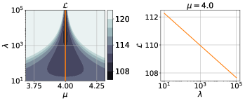
Figure 1: The NLL $\mathcal{L}$ of a Gaussian mixture model $p(y)=0.5\mathcal{N}(y\operatorname{;}0,1)+0.5\mathcal{N}(y\operatorname{;}\mu,\lambda^{-1})$ evaluated on $T=50$ data points with $y_{T}=4$.

Assumption 2.6 (Regularizers).

The regularizer $\mathcal{R}:\mathcal{X}_{\theta}\to\mathrm{I\!R}$ is separable in $\bm{\Theta},\bm{\beta}$, i.e., $\mathcal{R}(\theta)=\mathcal{R}_{1}(\bm{\Theta})+\mathcal{R}_{2}(\bm{\beta})$, and satisfies the following conditions

1. $\mathcal{R}_{1},\mathcal{R}_{2}$ are convex;

2. there exist $\kappa_{1},\kappa_{2}>0$ and $c_{1},c_{2}\in\mathrm{I\!R}$ such that for any $\bm{\xi}\in\Xi^{T+1}$:

$$\Psi_{\bm{\xi}}(\bm{\Theta}) +\mathcal{R}_{1}(\bm{\Theta}) \geq \;\kappa_{1}\|\bm{\Theta}\| \,+\,c_{1},$$ (13a)

$$\Phi_{\bm{\xi}}(\bm{\beta}) +\mathcal{R}_{2}(\bm{\beta}) \geq \;\kappa_{2}\|\bm{\beta}\| \,+\,c_{2}.$$ (13b)

In the upcoming analysis, we demonstrate that Assumption 2.6 prevents the scenario described in Example 2.5. A common regularizer satisfying (13a) is a quadratic function. However, the selection of $\mathcal{R}_{2}$ to satisfy (13b) depends on the specific form of $f,\ell_{t}$, and $g_{t}$. A potential candidate is the log-probability derived from the conjugate prior [11, §2.4.2], if it exists. To illustrate this, we present the following example.

Example 2.7 (Regularization for Gaussian distributions).

Consider 1b as a 1D Gaussian distribution. Recall from Table 1 that for $t\geq 0$

$$\textstyle f(\ell_{t}(\beta_{i}))+g_{{t}}(\beta_{i})=\frac{1}{2\lambda_{i}}(\lambda_{i}y_{t+1}-b_{i}z_{t})^{2}-\frac{1}{2}\ln\lambda_{i}$$

for all $i\in\Xi$. Thus, by (12c), $\Phi_{\bm{\xi}}(\bm{\beta})\geq\sum_{t=0}^{T-1}-\frac{1}{2}\ln\lambda_{\xi_{t+1}}$. Let $\mathcal{R}_{2}(\bm{\beta})=\frac{1}{2}\sum_{j=1}^{d}\lambda_{j}-\ln\lambda_{j}+b_{j}^{2}/\lambda_{j}$, which is derived from the conjugate prior of a Gaussian distribution [11, §2.3.6]. We first show that with this regularization, there exists some $\kappa>0$, such that for all sequence $\bm{\xi}\in\Xi^{T+1}$,

$$\textstyle\sum_{t=0}^{T-1}\!-\frac{1}{2}\ln\!\lambda_{\xi_{t+1}}\!+\mathcal{R}_{2}(\bm{\beta})\geq c+\kappa\sum_{j=1}^{d}\left\lvert b_{j}\right\rvert+\left\lvert\lambda_{j}\right\rvert.$$ (14)

This is equivalent showing for any $\alpha>0$, there exists $\kappa>0$ such that for all $a>0$,

$$u(\lambda,b)=-a\ln\lambda+\alpha\lambda+\alpha\tfrac{b^{2}}{\lambda}-\kappa\left\lvert b\right\rvert-\kappa\lambda$$

is lower bounded uniformly. By lower bounding the quadratic term of $b$, we obtain $u(\lambda,b)\geq-a\ln\lambda+\big{(}\alpha-\frac{1}{4\alpha}\kappa^{2}-\kappa\big{)}\lambda.$ This lower bound has a unique minimum for all $\lambda>0$ if $\alpha-\frac{1}{4\alpha}\kappa^{2}-\kappa>0$. Given $a,\alpha>0$, one can always choose $\kappa\in(0,2(\sqrt{2}-1)\alpha)$ to satisfy this condition. Thus, there exists $\kappa>0$ such that $u$ is lower-bounded. Because $\sum_{j=1}^{d}\left\lvert b_{j}\right\rvert+\left\lvert\lambda_{j}\right\rvert\geq\left\lVert\bm{\beta}\right\rVert=\sqrt{\sum_{j=1}^{d}\left\lvert b_{j}\right\rvert^{2}+\left\lvert\lambda_{j}\right\rvert^{2}}$, (14) implies that (13b) is satisfied.

It is evident from (11) and (12) that the NLL $\mathcal{L}$ is nonconvex, making problem (8) difficult to solve using off-the-shelf methods. Moreover, $\mathcal{L}$ entails the marginalization over a discrete sequence $\bm{\xi}$, of which the size grows exponentially with the horizon $T$. To prevent an exponential growth in computational complexity, evaluating $\mathcal{L}(\theta)$ typically involves a dynamic programming procedure, with a complexity proportional to the sequence length. However, due to the sequential nature of dynamic programming, each gradient evaluation $\nabla\mathcal{L}(\theta)$ must be propagated through the entire sequence $\bm{\xi}$ in order, leading to highly costly iterations. The goal of this work is therefore to develop a solution method that reduces the number of inherently expensive iterations by maximally exploiting the known structure of the problem class. By adopting the majorization-minimization (MM) principle [22, 30], with a majorization model that provides a tighter upper bound of the cost landscape, one can expect to make more progress per iteration than with general purpose (e.g., quadratic) models underlying classical gradient-based methods.

3 The identification method

This section introduces the proposed method EM++ as a particular MM scheme for minimizing the regularized NLL. An MM scheme iteratively performs two steps. The majorization step constructs a surrogate function $\bar{\mathcal{Q}}^{k}$ at the current iterate $\theta^{k}\in\mathcal{X}_{\theta}$, satisfying

$$\bar{\mathcal{Q}}^{k}(\theta)\geq \;\bar{\mathcal{L}}(\theta),\quad\forall\theta\in\mathcal{X}_{\theta},$$ (15a)

$$\bar{\mathcal{Q}}^{k}(\theta^{k})= \;\bar{\mathcal{L}}(\theta^{k}).$$ (15b)

The minimization step, consists of minimizing the surrogate function $\bar{\mathcal{Q}}^{k}$, yielding the next iterate $\theta^{k+1}$. In particular, we construct a convex surrogate function $\bar{\mathcal{Q}}^{k}$ satisfying (15), such that a sequence of convex problems is solved instead of the original nonconvex problem (8). The following lemma provides a first step towards the construction of such a surrogate function.

Lemma 3.1.

Let ${\bm{y}}$ be a trajectory of system (1) and $\theta^{k}\in\mathcal{X}_{\theta}$ an iterate. Then we can bound the NLL by

$$\mathcal{L}(\theta)\leq-\Pi(\theta^{k})^{\top}\left({\bm{c}}-\Psi(\bm{\Theta})-\Phi(\bm{\beta})\right)+c_{\theta^{k}}$$

with $c_{\theta^{k}}=\textstyle{\sum_{\bm{\xi}\in\Xi^{T+1}}}p(\bm{\xi}\mid\bm{y},z_{0}\operatorname{;}\theta^{k})\ln p(\bm{\xi}\mid\bm{y},z_{0}\operatorname{;}\theta^{k})$ and $\Pi(\theta^{k})\in\mathrm{I\!R}^{d^{T+1}}$ with element $\Pi_{\bm{\xi}}(\theta^{k})=p(\bm{\xi}\mid\bm{y},z_{0}\operatorname{;}\theta^{k})$ for all $\bm{\xi}\in\Xi^{T+1}$. Moreover, this relation holds with equality whenever $\theta=\theta^{k}$.

Proof.

Using (9) and Jensen’s inequality we have

$$\mathcal{L}(\theta) =-\ln\textstyle\sum_{\bm{\xi}\in\Xi^{T+1}}\tfrac{p(\bm{\xi}\mid\bm{y},z_{0}\operatorname{;}\theta^{k})}{p(\bm{\xi}\mid\bm{y},z_{0}\operatorname{;}\theta^{k})}p({\bm{y}},\bm{\xi},z_{0}\operatorname{;}\theta)$$

$$\leq-\textstyle\sum_{\bm{\xi}\in\Xi^{T+1}}p(\bm{\xi}\mid\bm{y},z_{0}\operatorname{;}\theta^{k})\ln\tfrac{p({\bm{y}},\bm{\xi},z_{0}\operatorname{;}\theta)}{p(\bm{\xi}\mid\bm{y},z_{0}\operatorname{;}\theta^{k})}$$

$$=-\textstyle\sum_{\bm{\xi}\in\Xi^{T+1}}p(\bm{\xi}\mid\bm{y},z_{0}\operatorname{;}\theta^{k})\ln p({\bm{y}},\bm{\xi},z_{0}\operatorname{;}\theta)+c_{\theta^{k}},$$

and this holds with equality for $\theta=\theta^{k}$. The claims follows from the observation that

$$\ln p({\bm{y}},\bm{\xi},z_{0}\operatorname{;}\theta)={\bm{c}}_{\bm{\xi}}-\Psi_{\bm{\xi}}(\bm{\Theta})-\Phi_{\bm{\xi}}(\bm{\beta}).\qed$$

By exploiting concavity of $f$, the next proposition constructs a surrogate $\bar{\mathcal{Q}}^{k}$ satisfying (15).

Proposition 3.2.

Let ${\bm{y}}$ be a trajectory of system (1) initialized at $z_{0}$. Then $\bar{\mathcal{Q}}^{k}(\theta):=\mathcal{Q}^{k}(\theta)+\mathcal{R}(\theta)$ with

$$\mathcal{Q}^{k}(\theta):=\mathcal{Q}^{k}_{0}+\mathcal{Q}^{k}_{1}(\bm{\Theta})+\mathcal{Q}^{k}_{2}(\bm{\beta}),$$ (16a)

constitutes a convex surrogate of $$\bar{\mathcal{L}}$$ satisfying (15), where

$$\mathcal{Q}^{k}_{0}{}\mathop{\mathrel{:}=}{} c_{\theta^{k}}-\Pi(\theta^{k})^{\top}{\bm{c}},$$ (16b)

$$\mathcal{Q}^{k}_{1}(\bm{\Theta}){}\mathop{\mathrel{:}=}{} \;\Pi(\theta^{k})^{\top}\Psi(\bm{\Theta}),$$ (16c)

$$\mathcal{Q}^{k}_{2}(\bm{\beta}){}\mathop{\mathrel{:}=}{} \;\Pi(\theta^{k})^{\top}\hat{\Phi}^{k}(\bm{\beta}),$$ (16d)

and where for all $\bm{\xi}\in\Xi^{T+1}$ we defined

$$\hat{\Phi}^{k}_{\bm{\xi}}(\bm{\beta}) {}\mathop{\mathrel{:}=}{}\textstyle\sum\limits_{t=0}^{T-1}f[\ell_{t}(\beta^{k}_{\xi_{t+1}})](\ell_{t}(\beta_{\xi_{t+1}}))+g_{{t}}(\beta_{\xi_{t+1}})$$ (17)

$$f[\bar{x}](x) {}\mathop{\mathrel{:}=}{}f(\bar{x})+f^{\prime}(\bar{x})(x-\bar{x}).$$

Proof.

By concavity of the function $f$, its linearization around a point $\bar{x}\in\operatorname{\mathbf{dom}}f$ constitutes an upper bound, i.e., for all $x\in\operatorname{\mathbf{dom}}f$: $f(x)\leq f(\bar{x})+f^{\prime}(\bar{x})(x-\bar{x})$, and this holds with equality when $x=\bar{x}$. Therefore, we have that $\Phi_{\bm{\xi}}(\bm{\beta})\leq\hat{\Phi}^{k}_{\bm{\xi}}(\bm{\beta})$, with equality holding for $\bm{\beta}=\bm{\beta}^{k}$. In combination with the bound from Lemma 3.1, this proves the claim. ∎

As the mappings $\Psi$, $g_{t}$, $\ell_{t}$, and $\mathcal{R}$ are convex, so is the surrogate problem $\operatorname*{\arg\!\min}_{\theta}\bar{\mathcal{Q}}^{k}(\theta)$. We remark that the direct computation of $\mathcal{Q}^{k}$ based on 16 is expensive, as it involves evaluating the vector $\Pi(\theta^{k})$ of dimension $d^{T+1}$. Section 5 describes a different representation of $\mathcal{Q}^{k}$ (cf. Proposition 5.1) that allows for efficient evaluation, once certain quantities are computed (cf. Algorithm 2). Exploiting separability of $\mathcal{Q}^{k}$ and $\mathcal{R}$ w.r.t. $\bm{\Theta},\bm{\beta}$, the resulting scheme is summarized in Algorithm 1.

Algorithm 1 EM++

1:Data ${\bm{y}}$; Initialize $\theta^{0}\in\mathcal{X}_{\theta}$

2:for $k=0,1,\dots$ (until convergence) do

3:     Run Algorithm 2 to construct $\mathcal{Q}^{k}_{1},\mathcal{Q}^{k}_{2}$

4:     Solve (in parallel)

$$\bm{\Theta}^{k+1}\leftarrow \;\textstyle\operatorname*{\arg\!\min}_{\bm{\Theta}}\mathcal{Q}^{k}_{1}(\bm{\Theta})+\mathcal{R}_{1}(\bm{\Theta})$$ (18a)

$$\bm{\beta}^{k+1}\leftarrow \;\textstyle\operatorname*{\arg\!\min}_{\bm{\beta}}\mathcal{Q}^{k}_{2}(\bm{\beta})\,\,+\mathcal{R}_{2}(\bm{\beta})$$ (18b)

5:end for

We highlight that the loss evaluated at $\{\theta^{k}\}_{k\in\mathrm{I\!N}}$ from EM++ is nonincreasing, as formally stated below.

Corollary 3.3 (Nonincreasing sequence).

The iterates $\{\theta^{k}\}_{k\in\mathrm{I\!N}}$ generated by EM++ (cf. Algorithm 1) satisfy

$$\forall k\in\mathrm{I\!N}:\bar{\mathcal{L}}(\theta^{k})\geq\bar{\mathcal{L}}(\theta^{k+1}).$$ (19)

Proof.

By Proposition 3.2, (15) holds, and we have

$$\forall k\in\mathrm{I\!N}:\bar{\mathcal{L}}(\theta^{k+1})\leq\bar{\mathcal{Q}}^{k}(\theta^{k+1})\leq\bar{\mathcal{Q}}^{k}(\theta^{k})=\bar{\mathcal{L}}(\theta^{k}).\qed$$

4 Convergence analysis

4.1 Subsequential convergence

We start by presenting two lemmata that will prove useful in the upcoming convergence analysis. The first states that the loss function $\bar{\mathcal{L}}$ is lower bounded, and that solutions to the surrogate problems $\operatorname*{\arg\!\min}_{\theta}\bar{\mathcal{Q}}^{k}(\theta)$ remain in a compact set. The second relates to the directional differentiability of $\bar{\mathcal{L}}$ and $\bar{\mathcal{Q}}{}$.

Lemma 4.1.

Under Assumptions 2.1 and 2.6,

1. $\bar{\mathcal{L}}$ is lower bounded;

2. there exists a compact set $\Omega\subseteq\mathcal{X}_{\theta}$ that contains the iterates $\left\{\theta^{k}\right\}_{k\in\mathrm{I\!N}}$ generated by EM++ (cf. Algorithm 1).

Proof.

By Assumption 2.6, 12c and 12b we have

$$\min_{\bm{\xi}\in\Xi^{T+1}}\Psi_{\bm{\xi}}(\bm{\Theta})\, + \,\mathcal{R}_{1}(\bm{\Theta}) \,\geq \,\kappa_{1}\left\lVert\bm{\Theta}\right\rVert +\,c_{1},$$

$$\min_{\bm{\xi}\in\Xi^{T+1}}\Phi_{\bm{\xi}}(\bm{\beta})\, + \,\mathcal{R}_{2}(\bm{\beta}) \,\geq \,\kappa_{2}\left\lVert\bm{\beta}\right\rVert +\,c_{2}.$$

Following from $\mathrm{lse}(x)\leq\max_{i}x_{i}+\ln n_{x}$,

$$\bar{\mathcal{L}}(\theta)= \;-\mathrm{lse}\left({\bm{c}}-\Psi(\bm{\Theta})-\Phi(\bm{\beta})-\mathcal{R}(\theta)\right)$$

$$\geq \;\min_{\bm{\xi}\in\Xi^{T+1}}-{\bm{c}}_{\bm{\xi}}+\Psi_{\bm{\xi}}(\bm{\Theta})+\Phi_{\bm{\xi}}(\bm{\beta})+\mathcal{R}(\theta)-\ln d^{T+1},$$

where $\mathcal{R}(\theta)=\mathcal{R}_{1}(\bm{\Theta})+\mathcal{R}_{2}(\bm{\beta})$. Thus, there exist $\kappa_{3}>0$, $c_{3}\in\mathrm{I\!R}$ for which

$$\bar{\mathcal{L}}(\theta) \geq\kappa_{1}\|\bm{\Theta}\|+\kappa_{2}\|\bm{\beta}\|+c_{3}\geq\kappa_{3}\|\theta\|+c_{3},$$

and the last step follows by equivalence of norms in Euclidean spaces, demonstrating that $\bar{\mathcal{L}}$ is bounded below and that $\liminf_{\|\theta\|\to\infty}\frac{\bar{\mathcal{L}}(\theta)}{\|\theta\|}=\kappa_{3}>0.$ Thus, $\bar{\mathcal{L}}$ is level-coercive [43, Definition 3.25], implying it has bounded level-sets [43, Corollary 3.27]. As shown in Corollary 3.3, the sequence $\left\{\bar{\mathcal{L}}(\theta^{k})\right\}_{k\in\mathrm{I\!N}}$ is nonincreasing. Hence, the iterates $\left\{\theta^{k}\right\}_{k\in\mathrm{I\!N}}$ remain in the bounded level-set $\Omega{}\mathop{\mathrel{:}=}{}\left\{\theta\mid\bar{\mathcal{L}}(\theta)\leq\bar{\mathcal{L}}(\theta^{0})\right\}\in\mathcal{X}_{\theta}$. By continuity of $\bar{\mathcal{L}}$, $\Omega$ is closed [43, Theorem 1.6(c)], and thus compact. ∎

Lemma 4.2.

If Assumptions 2.1 and 2.6 hold, then $\bar{\mathcal{L}}$ and $\bar{\mathcal{Q}}{}$ are directionally differentiable at $\theta^{k}$ along any $v=(v_{\bm{\Theta}},v_{\bm{\beta}})\in\mathbb{T}$. Moreover,

$$\bar{\mathcal{L}}^{\prime}(\theta^{k}\operatorname{;}v)=\bar{\mathcal{Q}}^{k^{\prime}}(\theta^{k}\operatorname{;}v).$$

Proof.

Denote $L_{\bm{\xi}}(\theta)={\bm{c}}_{\bm{\xi}}-\Psi_{\bm{\xi}}(\bm{\Theta})-\Phi_{\bm{\xi}}(\bm{\beta})$ for all $\bm{\xi}\in\Xi^{T+1}$, such that $\mathcal{L}(\theta)=-\mathrm{lse}(L(\theta))$. Under Assumption 2.1 the functions $\ell_{t},g_{t}$, and $-f$ are strictly continuous and convex ($f$ is concave). Since convexity ensures directional differentiability[42, Th. 23.1], it follows that $f,\ell_{t},g_{t}$ are B-differentiable on their domains [20, Definition 3.1.2]. Then, by the composition rule [20, proposition 3.1.6] also $\mathcal{L}$ is B-differentiable on its domain, and for all $v\in\mathbb{T}$ the directional derivative at $\theta$ along $v$ equals

$$\mathcal{L}^{\prime}(\theta\operatorname{;}v) =-\mathrm{lse}^{\prime}\Big{(}L(\theta)\operatorname{;}L^{\prime}(\theta\operatorname{;}v)\Big{)}=-\langle\nabla\mathrm{lse}\left(L(\theta)\right),L^{\prime}(\theta\operatorname{;}v)\rangle$$

$$=\Big{\langle}\nabla\mathrm{lse}\left(L(\theta)\right),\Psi^{\prime}(\bm{\Theta}\operatorname{;}v_{\bm{\Theta}})+\Phi^{\prime}(\bm{\beta}\operatorname{;}v_{\bm{\beta}})\Big{\rangle}.$$ (20)

Since by (9) and (11) we have $L_{\bm{\xi}}(\theta)=\ln p(\bm{y},\bm{\xi},z_{0}\operatorname{;}\theta),$ it follows that $\exp(L_{\bm{\xi}}(\theta))=p(\bm{y},\bm{\xi},z_{0}\operatorname{;}\theta).$ As the gradient of $\mathrm{lse}$ is the softmax function, i.e., $\nabla\mathrm{lse}\left(L(\theta)\right)=\sigma(L(\theta)),$ it follows that

$$\sigma_{\bm{\xi}}(L(\theta))= \;\frac{p(\bm{y},\bm{\xi},z_{0}\operatorname{;}\theta)}{\sum_{\bm{\xi}^{\prime}\in\Xi^{T+1}}p(\bm{y},\bm{\xi}^{\prime},z_{0}\operatorname{;}\theta)}$$

$$= \;\frac{p(\bm{y},\bm{\xi},z_{0}\operatorname{;}\theta)}{p({\bm{y}},z_{0}\operatorname{;}\theta)}=p(\bm{\xi}\mid{\bm{y}},z_{0}\operatorname{;}\theta)=\Pi_{\bm{\xi}}(\theta)$$

for all $\bm{\xi}\in\Xi^{T+1}$. We thus obtain that

$$\mathcal{L}^{\prime}(\theta^{k}\operatorname{;}v)=\Pi(\theta^{k})^{\top}\left(\Psi^{\prime}(\bm{\Theta}^{k}\operatorname{;}v_{\bm{\Theta}})+\Phi^{\prime}(\bm{\beta}^{k}\operatorname{;}v_{\bm{\beta}})\right).$$

On the other hand, we have by definition of $\mathcal{Q}^{k}$ that

$$\mathcal{Q}^{k^{\prime}}(\theta^{k}\operatorname{;}v)=\Pi(\theta^{k})^{\top}\left(\Psi^{\prime}(\bm{\Theta}^{k}\operatorname{;}v_{\bm{\Theta}})+\hat{\Phi}^{k^{\prime}}(\bm{\beta}^{k}\operatorname{;}v_{\bm{\beta}})\right).$$

At any point $\bar{x}\in\operatorname{\mathbf{dom}}f$, the derivative of $f$ equals the derivative of its linearization around $\bar{x}$, i.e., $f^{\prime}(\bar{x})=[f(\bar{x})+f^{\prime}(\bar{x})(\cdot-\bar{x})]^{\prime}(\bar{x}).$ It follows that $\Phi_{\bm{\xi}}^{\prime}(\bm{\beta}^{k}\operatorname{;}v_{\bm{\beta}})=\hat{\Phi}^{k^{\prime}}_{\bm{\xi}}(\bm{\beta}^{k}\operatorname{;}v_{\bm{\beta}})$ for all $\bm{\xi}\in\Xi^{T+1}$, and hence that $\mathcal{L}^{\prime}(\theta^{k}\operatorname{;}v)=\mathcal{Q}^{k^{\prime}}(\theta^{k}\operatorname{;}v)$ for all $v\in\mathbb{T}$. Since $\mathcal{R}$ is convex, it is also directionally differentiable [42, Theorem 23.1]. Thus, $\bar{\mathcal{L}}=\mathcal{L}+\mathcal{R}$ and $\bar{\mathcal{Q}}^{k}=\mathcal{Q}^{k}+\mathcal{R}$ are directionally differentiable on their domain and for all $v\in\mathbb{T}$ we obtain that $\bar{\mathcal{L}}^{\prime}(\theta^{k}\operatorname{;}v)=\bar{\mathcal{Q}}^{k^{\prime}}(\theta^{k}\operatorname{;}v).$ ∎

Theorem 4.3 (Subsequential convergence).

Under Assumptions 2.1 and 2.6, every limit point of the iterates $\left\{\theta^{k}\right\}_{k\in\mathrm{I\!N}}$ generated by EM++ (cf. Algorithm 1) is a stationary point of $\bar{\mathcal{L}}$.

Proof.

The proof follows [41, Theorem 1]. By Assumption 2.6 and Lemma 4.1, all iterates $\theta^{k}$ stay in a compact set $\Omega$. Thus, there exists a subsequence $\{\theta^{k_{j}}\}_{{k_{j}}\in\mathcal{K}\subseteq\mathrm{I\!N}}$ that converges to some $\theta^{\infty}\in\Omega$. It satisfies

$$\;\bar{\mathcal{Q}}^{k_{j+1}}(\theta^{k_{j+1}})=\bar{\mathcal{L}}(\theta^{k_{j+1}})\leq\bar{\mathcal{L}}(\theta^{k_{j}+1})$$ (21)

$$\;\quad\quad\leq\bar{\mathcal{Q}}^{k_{j}}(\theta^{k_{j}+1})\leq\bar{\mathcal{Q}}^{k_{j}}(\theta),\quad\forall\theta\in\mathbb{T},$$

where we consecutively used (15b), (19), and (15a). Taking the limit as $k\to\infty$ yields

$$-\infty<\bar{\mathcal{L}}(\theta^{\infty})=\bar{\mathcal{Q}}^{\infty}(\theta^{\infty})\leq\bar{\mathcal{Q}}^{\infty}(\theta),\quad\forall\theta\in\mathbb{T}.$$ (22)

The last inequality implies that $\theta^{\infty}$ is a (global) minimizer of $\bar{\mathcal{Q}}^{\infty}$. By the first-order necessary conditions of optimality we therefore have that $(\bar{\mathcal{Q}}^{\infty})^{\prime}(\theta^{\infty}\operatorname{;}v)\geq 0,$ for all $v\in\mathbb{T}$. Thus, $\theta^{\infty}$ is a stationary point of $\bar{\mathcal{L}}$, since by Lemma 4.2 we have $\bar{\mathcal{L}}^{\prime}(\theta^{\infty}\operatorname{;}v)\geq 0,$ for all $v\in\mathbb{T}$. ∎

4.2 Global sequential convergence

Interpreting EM++ (cf. Algorithm 1) as a mirror descent method, this section establishes global sequential convergence under a slightly more restrictive assumption.

Assumption 4.4.

We assume that

1. $\ell_{t}$ and $g_{t}$ are Lipschitz smooth on any compact set $\Omega_{\theta}\subseteq\mathcal{X}_{\theta}$ for all $t\in\mathrm{I\!N}_{[0,T-1]}$;

2. $f$ is Lipschitz smooth on any compact set $\Omega_{f}\subseteq\mathcal{X}_{f}$;

3. the regularizer $\mathcal{R}$ is of class $\mathcal{C}^{2}$ with $\nabla^{2}\mathcal{R}(\theta)\succ 0$ for all $\theta\in\mathcal{X}_{\theta}$.

We briefly introduce Bregman distances, which play a central role in the context of mirror descent methods.

Definition 4.5 (Bregman distance [14]).

For a convex function $h:\mathrm{I\!R}^{n}\rightarrow\mathrm{I\!R}\cup\{\infty\}$, which is continuously differentiable on $\operatorname{\mathbf{int\,dom}}h\neq\emptyset$, the Bregman distance $D_{h}:\mathrm{I\!R}^{n}\times\mathrm{I\!R}^{n}\rightarrow\overline{\mathrm{I\!R}}$ is given by

$$D_{h}(x,\tilde{x}){}\mathop{\mathrel{:}=}{}\begin{cases}h(x)-h(\tilde{x})-\langle\nabla h(\tilde{x}),x-\tilde{x}\rangle&\text{if}\;\tilde{x}\in\operatorname{\mathbf{int\,dom}}{h}\\ \infty&\text{otherwise.}\end{cases}$$

We say that the Bregman distance $D_{h}$ is induced by the kernel function $h$. Examples include 1 the Euclidean distance with $h(x)=\left\lVert x\right\rVert^{2}$; and 2 the Kullback-Leibler divergence with $h(p)=\sum_{i}p_{i}\ln p_{i}$ being the negative entropy function. The mirror-descent method [6] generalizes classical gradient descent method, which, when applied to (8), can be written as

$$\theta^{k+1}=\operatorname*{\arg\!\min}_{\theta}\bar{\mathcal{L}}(\theta^{k})+\langle\nabla\bar{\mathcal{L}}(\theta^{k}),\theta-\theta^{k}\rangle+\tfrac{1}{2}\|\theta-\theta^{k}\|^{2}.$$

The mirror descent method replaces the quadratic term $\tfrac{1}{2}\|\theta-\theta^{k}\|^{2}$ by some Bregman distance $D_{h}(\theta,\theta^{k})$. We now show that EM++ (cf. Algorithm 1) can be interpreted as a mirror descent method for solving the problem (8).

Proposition 4.6 (Mirror descent interpretation).

Consider the iterates $\left\{\theta^{k}\right\}_{k\in\mathrm{I\!N}}$ generated by EM++ (cf. Algorithm 1). Under Assumptions 2.1, 2.6 and 4.4 we have

$$\theta^{k+1}=\operatorname*{\arg\!\min}_{\theta}\bar{\mathcal{L}}(\theta^{k})+\langle\nabla\bar{\mathcal{L}}(\theta^{k}),\theta-\theta^{k}\rangle+D_{h^{k}}\left(\theta,\theta^{k}\right)$$ (23)

for all $k\in\mathrm{I\!N}$, where $h^{k}$ is a strictly convex function

$$h^{k}(\theta) {}\mathop{\mathrel{:}=}{}\mathcal{Q}^{k}_{1}(\bm{\Theta})+\mathcal{Q}^{k}_{2}(\bm{\beta})+\mathcal{R}(\theta).$$ (24)

Proof.

Algorithm 1 computes $\theta^{k+1}=\operatorname*{\arg\!\min}_{\theta}\bar{\mathcal{Q}}^{k}(\theta)$. From (15b), we know that $\bar{\mathcal{Q}}^{k}(\theta^{k})=\bar{\mathcal{L}}(\theta^{k})$. It therefore remains to show that

$$\bar{\mathcal{Q}}^{k}(\theta)=\bar{\mathcal{Q}}^{k}(\theta^{k})+\langle\nabla\bar{\mathcal{L}}({\theta^{k}}),\theta-\theta^{k}\rangle+D_{h^{k}}\big{(}\theta,{\theta^{k}}\big{)}.$$ (25)

Under Assumption 4.4, the functions $\bar{\mathcal{Q}}^{k}$, $\bar{\mathcal{L}}$ and $\mathcal{R}$ are differentiable. Consequently, Lemma 4.2 implies that $\nabla\bar{\mathcal{L}}(\theta^{k})=\nabla\bar{\mathcal{Q}}^{k}(\theta^{k})$, and by definition of $\bar{\mathcal{Q}}^{k}$ we have

$$\langle\nabla\bar{\mathcal{L}}({\theta^{k}}), \theta-\theta^{k}\rangle=\langle\nabla\mathcal{Q}^{k}_{1}(\bm{\Theta}^{k}),\bm{\Theta}-\bm{\Theta}^{k}\rangle$$

$$+\langle\nabla\mathcal{Q}^{k}_{2}(\bm{\beta}^{k}),\bm{\beta}-\bm{\beta}^{k}\rangle+\langle\nabla\mathcal{R}(\theta^{k}),\theta-\theta^{k}\rangle.$$

Thus, we obtain that

$$\bar{\mathcal{Q}}^{k}(\theta)- \bar{\mathcal{Q}}^{k}(\theta^{k})-\langle\nabla\bar{\mathcal{L}}(\theta^{k}),\theta-\theta^{k}\rangle$$

$$= D_{\mathcal{Q}^{k}_{1}}(\bm{\Theta},\bm{\Theta}^{k})+D_{\mathcal{Q}^{k}_{2}}(\bm{\beta},\bm{\beta}^{k})+D_{\mathcal{R}}(\theta,\theta^{k})$$

$$= D_{h^{k}}\left(\theta,\theta^{k}\right),$$

where the last step follows from [5, Prop. 3.5]. This proves (25) and concludes the proof. ∎

The convergence analysis of mirror descent-like methods typically relies on a descent lemma, see e.g., [4, Lemma 1], [13, Lemma 2.1]. The following lemma describes a similar relation for EM++ with respect to the variable kernel Bregman distance from Proposition 4.6.

Lemma 4.7 (Descent lemma).

Consider the iterates $\left\{\theta^{k}\right\}_{k\in\mathrm{I\!N}}$ generated by EM++ (cf. Algorithm 1). Under Assumptions 2.1, 2.6 and 4.4, we have for all $k\in\mathrm{I\!N}$ that

$$\bar{\mathcal{L}}(\theta^{k+1})\leq\bar{\mathcal{L}}(\theta^{k})+\langle\nabla\bar{\mathcal{L}}(\theta^{k}),\theta^{k+1}-\theta^{k}\rangle+D_{h^{k}}\left(\theta^{k+1},\theta^{k}\right).$$

Proof.

Immediate from (25), (15a), and (15b). ∎

We emphasize that the kernel function $h^{k}$ in 23 and 4.7 depends on the iterate $\theta^{k}$. In contrast to the analyses of mirror-descent like methods in [29, 13], where the kernel function is iterate-invariant, this dependency introduces a significant challenge in showing asymptotic convergence. Akin to [13], which proves global sequential convergence of so-called gradient-like descent sequences under a KL property, we show in the next lemma that the iterates of EM++ constitute such a sequence, despite the variable kernel functions.

Lemma 4.8.

Under Assumptions 2.1, 2.6 and 4.4, the sequence $\{\theta^{k}\}$ generated by EM++ (cf. Algorithm 1) is a gradient-like descent sequence for $\bar{\mathcal{L}}$, i.e.,

1. There exists a positive scalar $\rho_{1}$ such that $\rho_{1}\left\lVert\theta^{k+1}-\theta^{k}\right\rVert^{2}\leq\bar{\mathcal{L}}(\theta^{k})-\bar{\mathcal{L}}(\theta^{k+1})$ for all $k\in\mathrm{I\!N}$;

2. There exists a positive scalar $\rho_{2}$ such that $\left\lVert\nabla\bar{\mathcal{L}}(\theta^{k+1})\right\rVert\leq\rho_{2}\left\lVert\theta^{k+1}-\theta^{k}\right\rVert$ for all $k\in\mathrm{I\!N}$;

3. Let $\bar{\theta}$ be a limit point of a subsequence $\{\theta^{k}\}_{k\in\mathcal{K}}$, then $\lim\sup_{k\in\mathcal{K}\subset\mathrm{I\!N}}\bar{\mathcal{L}}(\theta^{k})\leq\bar{\mathcal{L}}(\bar{\theta})$.

Proof.

The optimality conditions defining (23) yield

$$\nabla\bar{\mathcal{L}}(\theta^{k})=\nabla h^{k}(\theta^{k})-\nabla h^{k}(\theta^{k+1}).$$ (26)

By Lemma 4.7 and Definition 4.5 this yields

$$\bar{\mathcal{L}}(\theta^{k+1})-\bar{\mathcal{L}}(\theta^{k})\leq \;\langle\nabla h^{k}(\theta^{k})-\nabla h^{k}(\theta^{k+1}),\theta^{k+1}-\theta^{k}\rangle$$

$$\;\;+D_{h^{k}}(\theta^{k+1},\theta^{k})$$

$$= \;\;-D_{h^{k}}(\theta^{k},\theta^{k+1}).$$ (27)

By (24), we have for all $\theta,\tilde{\theta}\in\mathcal{X}_{\theta}$,

$$\langle\nabla h^{k}(\theta)-\nabla h^{k}(\tilde{\theta}),\theta-\tilde{\theta}\rangle= \;\langle\nabla\mathcal{Q}^{k}_{1}(\bm{\Theta})-\nabla\mathcal{Q}^{k}_{1}(\tilde{\bm{\Theta}}),\bm{\Theta}-\tilde{\bm{\Theta}}\rangle$$

$$\;+\langle\nabla\mathcal{Q}^{k}_{2}(\bm{\beta})-\nabla\mathcal{Q}^{k}_{2}(\tilde{\bm{\beta}}),\bm{\beta}-\tilde{\bm{\beta}}\rangle$$

$$\;+\langle\nabla\mathcal{R}(\theta)-\nabla\mathcal{R}(\tilde{\theta}),\theta-\tilde{\theta}\rangle$$

$$\geq \;\langle\nabla\mathcal{R}(\theta)-\nabla\mathcal{R}(\tilde{\theta}),\theta-\tilde{\theta}\rangle,$$

where the inequality follows from the convexity of $\mathcal{Q}^{k}_{1}$ and $\mathcal{Q}^{k}_{2}$. By [35, Proposition 1.1] $D_{h^{k}}(\theta,\theta^{k})\geq D_{\mathcal{R}}(\theta,\theta^{k}).$ Combined with (27), this yields $\bar{\mathcal{L}}(\theta^{k})-\bar{\mathcal{L}}(\theta^{k+1})\geq D_{\mathcal{R}}(\theta^{k},\theta^{k+1}).$ By Assumption 2.6 and Lemma 4.1, the iterates $\theta^{k}$ remain in a compact set $\Omega\subset\mathcal{X}_{\theta}$. Since $\nabla^{2}\mathcal{R}(\theta)$ is continuous and $\nabla^{2}\mathcal{R}(\theta)\succ 0$ for all $\theta$, as assumed in Assumption 4.4, the function $\mathcal{R}$ is locally strongly convex on $\Omega$. Hence, there exists a constant $\rho_{1}>0$, such that $\bar{\mathcal{L}}(\theta^{k})-\bar{\mathcal{L}}(\theta^{k+1})\geq\rho_{1}\left\lVert\theta^{k}-\theta^{k+1}\right\rVert^{2},$ proving Lemma LABEL:*lem: gradient_like_descent_sequence (a). As for the second claim, we have by (26) that $\nabla\bar{\mathcal{L}}(\theta^{k+1})=\nabla\bar{\mathcal{L}}(\theta^{k+1})-\nabla\bar{\mathcal{L}}(\theta^{k})-\nabla h^{k}(\theta^{k+1})+\nabla h^{k}(\theta^{k}),$ and hence

$$\left\lVert\nabla\bar{\mathcal{L}}(\theta^{k+1})\right\rVert\leq \;\phantom{+}\left\lVert\nabla\bar{\mathcal{L}}(\theta^{k+1})-\nabla\bar{\mathcal{L}}(\theta^{k})\right\rVert$$

$$+\left\lVert\nabla h^{k}(\theta^{k+1})-\nabla h^{k}(\theta^{k})\right\rVert.$$ (28)

By Assumption 4.4, the loss function is composed of Lipschitz smooth functions on the compact set $\Omega$ that contains all iterates $\left\{\theta^{k}\right\}$. Hence, there exists $L_{\Omega}>0$ such that $\left\lVert\nabla\bar{\mathcal{L}}(\theta^{k+1})-\nabla\bar{\mathcal{L}}(\theta^{k})\right\rVert\leq L_{\Omega}\left\lVert\theta^{k+1}-\theta^{k}\right\rVert.$ Moreover, by (24), we can bound the second term of (4.2) by

$$\left\lVert\nabla h^{k}(\theta^{k+1})-\nabla h^{k}(\theta^{k})\right\rVert\leq\left\lVert\nabla\mathcal{Q}^{k}_{1}(\bm{\Theta}^{k+1})-\nabla\mathcal{Q}^{k}_{1}(\bm{\Theta}^{k})\right\rVert$$

$$\;\;+\left\lVert\nabla\mathcal{Q}^{k}_{2}(\bm{\beta}^{k+1})-\nabla\mathcal{Q}^{k}_{2}(\bm{\beta}^{k})\right\rVert+\left\lVert\nabla\mathcal{R}(\theta^{k+1})-\nabla\mathcal{R}(\theta^{k})\right\rVert.$$

Using (16c) and the Cauchy-Schwarz inequality, we further bound

$$\;\left\lVert\nabla\mathcal{Q}^{k}_{1}(\bm{\Theta}^{k+1})-\nabla\mathcal{Q}^{k}_{1}(\bm{\Theta}^{k})\right\rVert$$ (29)

$$\;\quad\quad\leq\big{\lVert}\Pi(\theta^{k})\big{\rVert}\big{\lVert}\nabla\Psi(\bm{\Theta}^{k+1})-\nabla\Psi(\bm{\Theta}^{k})\big{\rVert}.$$

Recall that $\Pi(\theta^{k})\in[0,1]^{d^{T+1}}$, the gradient of function $\mathrm{lse}$ is Lipschitz continuous on the compact set $\Omega\in\mathcal{X}_{\theta}$. Consequently, $\Psi$ has Lipschitz continuous gradients on $\Omega$, and there exists a constant $M_{1,\Omega}>0$ such that $\left\lVert\nabla\mathcal{Q}^{k}_{1}(\bm{\Theta}^{k+1})-\nabla\mathcal{Q}^{k}_{1}(\bm{\Theta}^{k})\right\rVert\leq M_{1,\Omega}\left\lVert\bm{\Theta}^{k+1}-\bm{\Theta}^{k}\right\rVert$ for all $\theta^{k}\in\mathcal{X}_{\theta}$. In a similar way, let $G,F_{t},Z_{t}\in\mathrm{I\!R}^{d^{T+1}}$ with elements $G_{\bm{\xi}}(\bm{\beta})=\sum_{t=0}^{T-1}g_{t}(\beta_{\xi_{t+1}}),$ $Z_{t,\bm{\xi}}(\bm{\beta})=\ell_{t}(\beta_{\xi_{t+1}}),$ and $F_{t,\bm{\xi}}(\bm{\beta}^{k})=f^{\prime}(\ell_{t}(\beta^{k}_{\xi_{t+1}}))$ for all $\bm{\xi}\in\Xi^{T+1}$ and $t\in\mathrm{I\!N}_{[0,T-1]}$. Hence, $\nabla\hat{\Phi}^{k}(\bm{\beta})=\sum_{t=0}^{T-1}F_{t}(\bm{\beta}^{k})\nabla Z_{t}(\bm{\beta})+\nabla G(\bm{\beta})$. Using (16d), the triangle and Cauchy-Schwarz inequality, we further bound

$$\;\left\lVert\nabla\mathcal{Q}^{k}_{2}(\bm{\beta}^{k+1})-\nabla\mathcal{Q}^{k}_{2}(\bm{\beta}^{k})\right\rVert$$ (30)

$$\leq \;\big{\lVert}\Pi(\theta^{k})\textstyle\sum\limits_{t=0}^{T-1}F_{t}(\bm{\beta}^{k})\left(\nabla Z_{t}(\bm{\beta}^{k+1})-\nabla Z_{t}(\bm{\beta}^{k})\right)\big{\rVert}$$

$$\;+\big{\lVert}\Pi(\theta^{k})\left(\nabla G(\bm{\beta}^{k+1})-\nabla G(\bm{\beta}^{k})\right)\big{\rVert}$$

$$\leq \;\textstyle\sum\limits_{t=0}^{T-1}\left\lVert\Pi(\theta^{k})F_{t}(\bm{\beta}^{k})\right\rVert\left\lVert\nabla Z_{t}(\bm{\beta}^{k+1})-\nabla Z_{t}^{1}(\bm{\beta}^{k})\right\rVert$$

$$\;+\big{\lVert}\Pi(\theta^{k})\big{\rVert}\big{\lVert}\nabla G_{t}(\bm{\beta}^{k+1})-\nabla G_{t}(\bm{\beta}^{k})\big{\rVert}.$$

As assumed in Assumption 4.4, $Z_{t}$, $G$ have Lipschitz continuous gradients on $\Omega$. Since $\Pi(\theta^{k})\!\in\![0,1]^{d^{T+1}}$ and $F_{t}(\bm{\beta}^{k})\!\in\![0,\bar{u}]^{d^{T+1}}$, following from Assumption 2.1, (30) implies that there exists $M_{2,\Omega}\!>\!0$ such that $\left\lVert\nabla\mathcal{Q}^{k}_{2}(\bm{\beta}^{k+1})\!-\!\nabla\mathcal{Q}^{k}_{2}(\bm{\beta}^{k})\right\rVert\leq M_{2,\Omega}\left\lVert\bm{\beta}^{k+1}\!-\!\bm{\beta}^{k}\right\rVert$ for all $\theta^{k}\!\in\!\mathcal{X}_{\theta}$. Since $\mathcal{R}$ is of class $\mathcal{C}^{2}$ by Assumption 4.4, it has Lipschitz continuous gradients on $\Omega$. Thus, there exists a constant $\rho_{2}>0$ such that $\left\lVert\nabla\bar{\mathcal{L}}(\theta^{k+1})\right\rVert\leq\rho_{2}\left\lVert\theta^{k+1}-\theta^{k}\right\rVert$. This proves Lemma LABEL:*lem: gradient_like_descent_sequence (b). Finally, Lemma LABEL:*lem: gradient_like_descent_sequence (c) follows directly from the continuity of $\bar{\mathcal{L}}$ on the set $\Omega\subset\mathcal{X}_{\theta}$. ∎

Definition 4.9 (KL property [12, 34]).

A proper and lower semicontinuous function $\eta:\mathrm{I\!R}^{n}\to\mathrm{I\!R}\cup\{\infty\}$ satisfies the Kurdyka-Łojasiewicz (KL) property at $\bar{\theta}\in\mathcal{X}_{\theta}$ if there exists a concave KL function $\psi:[0,b]\to[0,+\infty)$ with $b>0$ and a neighborhood $U_{\bar{\theta}}$ such that

1. $\psi(0)=0$;

2. $\psi\in\mathcal{C}^{1}$, with $\psi^{\prime}>0$ on $(0,b)$;

3. $\forall\theta\in U_{\bar{\theta}}$: if $\eta(\bar{\theta})<\eta(\theta)<\eta(\bar{\theta})+b$, then $\psi^{\prime}(\eta(\theta)-\eta(\bar{\theta}))\mathbf{dist}(0,\partial\eta(\theta))\geq 1$.

The KL property is a mild requirement that holds for real-analytic and semi-algebraic functions, and subanalytic functions that are continuous on their domain [12]. In fact, for these first two classes of functions, the KL function of $\bar{\mathcal{L}}$ can be taken of the form $\psi(s)=cs^{1-\alpha}$, with $c>0,\alpha\in[0,1)$ [3]. We highlight that often $f,\ell_{t},g_{t}$ are real-analytic for $t\in\mathrm{I\!N}_{[0,T-1]}$. Since sums, products and compositions of real-analytic functions are real-analytic, $\bar{\mathcal{L}}$ trivially satisfies the KL property in such cases. The next theorem shows that if $\bar{\mathcal{L}}$ satisfies the KL property, the whole sequence of iterates converges with a rate depending on the specific form of the KL function.

Theorem 4.10 (Global convergence).

Consider the iterates $\{\theta^{k}\}_{k\in\mathrm{I\!N}}$ generated by EM++ (cf. Algorithm 1). If $\bar{\mathcal{L}}$ satisfies the KL property, and if Assumptions 2.1, 2.6 and 4.4 hold, then $\{\theta^{k}\}_{k\in\mathrm{I\!N}}$ converges to a stationary point, i.e.,

$$\lim_{k\to\infty}\theta^{k}=\theta^{\star},\quad\text{with }\nabla\bar{\mathcal{L}}(\theta^{\star})=0.$$

If, additionally, the KL function $\psi$ of $\bar{\mathcal{L}}$ is of the form $\psi(s)=cs^{1-\alpha}$ with $c>0,\alpha\in[0,1)$, then

1. if $\alpha=0$ then $\left\{\theta^{k}\right\}$ converges to $\theta^{\star}$ in a finite number of steps;

2. if $\alpha\in(0,1/2]$ then there exist $w>0$ and $\tau\in[0,1)$ such that $\|\theta^{k}-\theta^{\star}\|\leq\omega\tau^{k};$

3. if $\alpha\in(1/2,1)$ then there exist $\omega>0$ such that $\|\theta^{k}-\theta^{\star}\|\leq\omega k^{-\frac{1-\alpha}{2\alpha-1}}.$

Proof.

By Lemma 4.8, $\left\{\theta^{k}\right\}$ is a gradient-like descent sequence. The claims follow by [13, Theorem 6.2 & 6.3]. ∎

5 Efficient evaluation of the surrogate

An effective implementation of EM++ (cf. Algorithm 1) requires efficient evaluation of the surrogate function $\mathcal{Q}^{k}$. Despite the exponential complexity inherent in the definition of $\mathcal{Q}^{k}$ in (16), its evaluation can be accomplished efficiently using the following representation.

Proposition 5.1.

Given a trajectory ${\bm{y}}$ of system (1) that is initialized at $z_{0}$, the terms of $\mathcal{Q}^{k}(\theta)=\mathcal{Q}^{k}_{0}+\mathcal{Q}^{k}_{1}(\bm{\Theta})+\mathcal{Q}^{k}_{2}(\bm{\beta})$ as defined in (16) can be represented as

$$\mathcal{Q}^{k}_{0}{}\mathop{\mathrel{:}=}{} \;\!-\!\textstyle\sum\limits_{i\in\Xi}\!\pi_{0}^{i}(\theta^{k})\!\big{[}\ln p(\xi_{0}\!=\!i,z_{0})\!+\!T\ln C\big{]}\!+\!c_{\theta^{k}},$$ (31a)

$$\mathcal{Q}^{k}_{1}(\bm{\Theta}){}\mathop{\mathrel{:}=}{} \;\textstyle\sum\limits_{t=0}^{T-1}\textstyle\sum\limits_{i,j\in\Xi}\pi_{t}^{i,j}(\theta^{k})\Big{(}\mathrm{lse}\big{(}\Theta_{i}^{\top}z_{t}\big{)}-\Theta_{i,j}^{\top}z_{t}\Big{)},$$ (31b)

$$\mathcal{Q}^{k}_{2}(\bm{\beta}){}\mathop{\mathrel{:}=}{} \;\hat{c}_{\theta^{k}}{+}\textstyle\sum\limits_{t=0}^{T-1}\!\textstyle\sum\limits_{i\in\Xi}\!\pi_{t+1}^{i}(\theta^{k})\Big{(}f^{\prime}\big{(}\ell_{t}(\beta_{i}^{k})\big{)}\,\ell_{t}(\beta_{i})+g_{t}(\beta_{i})\Big{)},$$ (31c)

where we have used the shorthands

$$\vspace{-\baselineskip}\pi_{t}^{i}(\theta^{k}) {}\mathop{\mathrel{:}=}{}p(\xi_{t}=i\mid{\bm{y}},z_{0}\operatorname{;}\theta^{k});$$

$$\pi_{t}^{i,j}(\theta^{k}) {}\mathop{\mathrel{:}=}{}p(\xi_{t}=i,\xi_{t+1}=j\mid{\bm{y}},z_{0}\operatorname{;}\theta^{k});$$

and $\hat{c}_{\theta^{k}}=\sum_{t=0}^{T-1}\sum_{i\in\Xi}-\pi_{t+1}^{i}(\theta^{k})f^{\prime}(\ell_{t}(\beta_{i}^{k}))\,\ell_{t}(\beta_{i}^{k})+\\ \pi_{t+1}^{i}(\theta^{k})f(\ell_{t}(\beta^{k}_{i}))$.

Proof.

We recall that each entry $\Pi_{\bm{\xi}}(\theta^{k})=p(\bm{\xi}\mid\bm{y},z_{0}\operatorname{;}\theta^{k})=p(\xi_{0},\dots,\xi_{T}\mid\bm{y},z_{0}\operatorname{;}\theta^{k})$ for some $\bm{\xi}\in\Xi^{T+1}$. A distribution $p(\xi_{0}\mid\bm{y},z_{0}\operatorname{;}\theta^{k})$ can be obtained by marginalizing out the random variables $\xi_{1},\dots\xi_{T}$, i.e.,

$$p(\xi_{0}\mid\bm{y},z_{0}\operatorname{;}\theta^{k})=\textstyle\sum\limits_{(\xi_{1},\dots,\xi_{T})\in\Xi^{T}}p(\xi_{0},\dots,\xi_{T}\mid\bm{y},z_{0}\operatorname{;}\theta^{k}).$$

Considering $\mathcal{Q}^{k}_{0}$ from (16b), we can apply this marginalization since ${\bm{c}}$ only depends on the latent variable $\xi_{0}$:

$$\mathcal{Q}^{k}_{0}= \;c_{\theta^{k}}-\textstyle\sum\limits_{\bm{\xi}\in\Xi^{T+1}}\Pi_{\bm{\xi}}(\theta^{k}){\bm{c}}_{\bm{\xi}}$$

$$= \;c_{\theta^{k}}-\quad\textstyle\sum\limits_{\mathclap{(\xi_{0},\dots,\xi_{T})\in\Xi^{T+1}}}p(\xi_{0},\dots,\xi_{T}\mid\bm{y},z_{0}\operatorname{;}\theta^{k})[\ln p(\xi_{0},z_{0})+T\ln C]$$

$$= \;c_{\theta^{k}}-\;\;\textstyle\sum\limits_{\xi_{0}\in\Xi}p(\xi_{0}\mid\bm{y},z_{0}\operatorname{;}\theta^{k})[\ln p(\xi_{0},z_{0})+T\ln C]$$

This yields (31a). We apply the same approach to $\mathcal{Q}^{k}_{1},\mathcal{Q}^{k}_{2}$ from 16d and 16c. In particular, the terms of $\Psi_{\bm{\xi}}(\bm{\Theta})$ in (12b) only depends on $\xi_{t},\xi_{t+1}$, and the terms of $\hat{\Phi}_{\bm{\xi}}(\bm{\beta})$ in (17) only depends on $\xi_{t+1}$. By marginalizing out the other latent variables, we obtain 31c and 31b. ∎

Since the switching probability of $\xi_{t+1}$ depends on $\xi_{t}$, as evident from (1a), we utilize the forward-backward algorithm [40] to compute the distributions $\pi_{t+1}^{i}(\theta^{k})$, $\pi_{t}^{i,j}(\theta^{k})$. The standard forward-backward algorithm computes the posterior distribution of latent variables in a hidden Markov model. Unlike hidden Markov models where the observations $y_{t}$ are conditionally independent given the latent variable $\xi_{t}$, the dynamics of $y_{t}$ described in (1b) necessitates some modifications to the original forward-backward scheme, as we now formalize.

Proposition 5.2.

Let $\rho_{t}(\xi_{t},\xi_{t+1}\operatorname{;}\theta^{k}){}\mathop{\mathrel{:}=}{}p(\xi_{t},\xi_{t+1},{\bm{y}}_{t+1:T}\mid{\bm{y}}_{0:t},z_{0}\operatorname{;}\theta^{k})$. The posterior distributions expressed as

$$\pi_{t+1}^{i}(\theta^{k})= \;\textstyle\sum_{j\in\Xi}\pi^{j,i}_{t}(\theta^{k})$$ (32a)

$$\pi_{t}^{i,j}(\theta^{k})= \;\frac{\rho_{t}(\xi_{t}=i,\xi_{t+1}=j\operatorname{;}\theta^{k})}{\sum_{m,n\in\Xi^{2}}\rho_{t}(\xi_{t}=m,\xi_{t+1}=n\operatorname{;}\theta^{k})}$$ (32b)

can be computed with

$$\rho_{t}(\xi_{t},\xi_{t+1}\operatorname{;}\theta^{k})=\zeta_{t}(\xi_{t+1}\operatorname{;}\theta^{k})\,p(\xi_{t+1}\mid z_{t},\xi_{t}\operatorname{;}\bm{\Theta}^{k})\,\alpha_{t}(\xi_{t}\operatorname{;}\theta^{k}),$$ (32c)

where $$\alpha_{t}(\xi_{t}){}\mathop{\mathrel{:}=}{}p(\xi_{t}\mid{\bm{y}}_{0:t},z_{0}) \zeta_{t}(\xi_{t+1}){}\mathop{\mathrel{:}=}{}p({\bm{y}}_{t+1:T}\mid\xi_{t+1},z_{t}) q_{t-1}(\xi_{t}){}\mathop{\mathrel{:}=}{}p(\xi_{t}\mid{\bm{y}}_{0:t-1},z_{0}) \alpha_{t}(\xi_{t}) \zeta_{t}(\xi_{t+1}) t\in\mathrm{I\!N}_{[1,T]}$$, . Let . The probability and the likelihood are updated recursively for all through

$$q_{t-1}(\xi_{t}\operatorname{;}\theta^{k})=\! \;\textstyle\sum\limits_{\mathclap{\xi_{t-1}\in\Xi}}p(\xi_{t}\!\mid z_{t-1},\xi_{t-1}\!\operatorname{;}\bm{\Theta}^{k}\!)\alpha_{t-1}(\xi_{t-1}\!\operatorname{;}\theta^{k}\!),$$ (32d)

$$\alpha_{t}(\xi_{t}\operatorname{;}\theta^{k})= \;\frac{p(y_{t}\mid z_{t-1},\xi_{t}\operatorname{;}\bm{\beta}^{k})\,q_{t-1}(\xi_{t}\operatorname{;}\theta^{k})}{\sum_{\xi_{t}\in\Xi}p(y_{t}\mid z_{t-1},\xi_{t}\operatorname{;}\bm{\beta}^{k})q_{t-1}(\xi_{t}\!\operatorname{;}\!\theta^{k})},$$ (32e)

$$\zeta_{t-1}(\xi_{t}\operatorname{;}\theta^{k})= \;\textstyle\sum_{\xi_{t+1}\in\Xi}\zeta_{t}(\xi_{t+1}\operatorname{;}\theta^{k})\times$$ (32f)

$$\;\quad p(\xi_{t+1}\mid z_{t},\xi_{t}\operatorname{;}\bm{\Theta}^{k})\,p(y_{t}\mid z_{t-1},\xi_{t}\operatorname{;}\bm{\beta}^{k})$$

with initialization $\alpha_{0}(\xi_{0})$, $\zeta_{T}(\xi_{T+1})=1$.

Proof.

For brevity, we omit the dependence on $\theta^{k}$ as it is fixed for all computations involved in (32). Recall the definition of $\pi_{t+1}^{i}$, $\pi_{t}^{i,j}$ in Proposition 3.2, equation (32b) and (32a) directly follow from the definition of the conditional distribution and the marginalization. The distribution $\rho_{t}(\xi_{t},\xi_{t+1})$ can be factorized as

$$\rho_{t}(\xi_{t},\xi_{t+1})= \;p(\xi_{t},\xi_{t+1},{\bm{y}}_{t+1:T}\mid{\bm{y}}_{0:t},z_{0})$$ (33)

$$= \;p({\bm{y}}_{t+1:T}\mid\xi_{t+1},\xi_{t},{\bm{y}}_{0:t},z_{0})\times$$

$$\;p(\xi_{t+1}\mid\xi_{t},{\bm{y}}_{0:t},z_{0})\,p(\xi_{t}\mid{\bm{y}}_{0:t},z_{0}).$$

Recall from (2) that $z_{t}$ is the trajectory history. Given $\xi_{t},z_{t}$, the distribution of $\xi_{t+1}$ is independent of ${\bm{y}}_{0:t-t_{y}}$ (cf. (1a)). Hence, $p(\xi_{t+1}\mid\xi_{t},{\bm{y}}_{0:t},z_{0})=p(\xi_{t+1}\mid z_{t},\xi_{t})$. Likewise, the future trajectory ${\bm{y}}_{t+1:T}$ is independent of the past trajectory ${\bm{y}}_{0:t-t_{y}}$. Thus, $p({\bm{y}}_{t+1:T}\mid\xi_{t+1},\xi_{t},{\bm{y}}_{0:t},z_{0})$ simplifies to $p({\bm{y}}_{t+1:T}\mid\xi_{t+1},z_{t})$. By definition of $\alpha_{t}(\xi_{t})$ and $\zeta_{t}(\xi_{t+1})$, (33) is equivalent to (32c).

By definition of $\alpha_{t}(\xi_{t})$ and $q_{t-1}(\xi_{t})$, (32d) directly follows from the law of total probability. Recall that

$$\alpha_{t}(\xi_{t}){}\mathop{\mathrel{:}=}{}p(\xi_{t}\mid{\bm{y}}_{0:t},z_{0})=\frac{p(y_{t},\xi_{t}\mid{\bm{y}}_{0:t-1},z_{0})}{p(y_{t}\mid{\bm{y}}_{0:t-1},z_{0})},$$ (34)

where the denominator $p(y_{t}\mid{\bm{y}}_{0:t-1},z_{0})\!=\!\sum_{\xi_{t}\in\Xi}p(y_{t},\xi_{t}\mid{\bm{y}}_{0:t-1},z_{0})$, and the numerator $p(y_{t},\xi_{t}\mid{\bm{y}}_{0:t-1})\!=\!p(y_{t}\mid\xi_{t},{\bm{y}}_{0:t-1},z_{0})p(\xi_{t}\mid{\bm{y}}_{0:t-1},z_{0})$, Given $\xi_{t}$ and $z_{t-1}$, $y_{t}$ is independent of the trajectory ${\bm{y}}_{0:t-t_{y}-1}$. Thus, $p(y_{t}\mid\xi_{t},{\bm{y}}_{0:t-1},z_{0})\!=\!p(y_{t}\mid z_{t-1},\xi_{t})$. Plugging this equation and the definition of $q_{t-1}(\xi_{t})$ in (34) yields (32e).

The likelihood $\zeta_{t-1}(\xi_{t})$ is obtained via marginalization:

$$\zeta_{t-1}(\xi_{t})\!{}\mathop{\mathrel{:}=}{}p({\bm{y}}_{t:T}\!\mid\!\xi_{t},z_{t-1})=\textstyle\sum\limits_{\mathclap{\xi_{t{+}1}\!\in\Xi}}p({\bm{y}}_{t:T},\xi_{t+1}\mid\xi_{t},z_{t-1})$$ (35)

where $p({\bm{y}}_{t:T},\xi_{t+1}\mid\xi_{t},z_{t-1})$ can be factorized as

$$p({\bm{y}}_{t:T},\xi_{t+1}\mid\xi_{t},z_{t-1}) =p({\bm{y}}_{t+1:T}\mid\xi_{t+1},\xi_{t},y_{t},z_{t-1})\times$$

$$p(\xi_{t+1}\mid\xi_{t},y_{t},z_{t-1})p(y_{t}\mid\xi_{t},z_{t-1}).$$

As $z_{t}$ is a function of the trajectory history, $p(\xi_{t+1}\mid\xi_{t},y_{t},z_{t-1})=p(\xi_{t+1}\mid z_{t},\xi_{t})$. Applying the definition of $\zeta_{t}$ and (1) in (35) yields (32f). ∎

Remark 5.3 (State-dependent switching).

A special case arises when the switching probability only depends on the trajectory history, as in (5), where the distribution $p(\xi_{t+1}\mid\xi_{t},z_{t}\operatorname{;}\theta^{k})=p(\xi_{t+1}\mid z_{t}\operatorname{;}\theta^{k})$ for $t\in\mathrm{I\!N}_{[0,T-1]}$. In this case, the posterior distribution

$$\pi_{t+1}^{i}\!(\theta^{k}\!)\!=\!p(\xi_{t+1}{=}i\!\mid\!{\bm{y}},z_{0}\!\operatorname{;}\!\theta^{k}\!)\!=\!\frac{p(y_{t+1},\xi_{t+1}{=}i\mid z_{t}\!\operatorname{;}\!\theta^{k}\!)}{p(y_{t+1}\mid z_{t}\!\operatorname{;}\theta^{k})},$$ (36)

with $p(y_{t+1},\xi_{t+1}\mid z_{t}\operatorname{;}\theta^{k})=p(y_{t+1}\mid\xi_{t+1},z_{t}\operatorname{;}\theta^{k})p(\xi_{t+1}\mid z_{t}\operatorname{;}\theta^{k})$. The joint distribution $\pi_{t}^{i,j}(\theta^{k})=p(\xi_{t}=i,\xi_{t+1}=j\mid{\bm{y}},z_{0}\operatorname{;}\theta^{k})=p(\xi_{t}=i\mid{\bm{y}},z_{0}\operatorname{;}\theta^{k})\,p(\xi_{t+1}=j\mid{\bm{y}},z_{0}\operatorname{;}\theta^{k})$ as a result of conditional independence. The computational complexity of (36) is $\mathcal{O}(dT)$. In contrast, the computation of (32) has a complexity of $\mathcal{O}(d^{2}T)$. Leveraging the independence in (36) is thus more efficient, especially when the number of modes $d$ is large. In addition, we highlight that (36) enables parallel computation across all $\xi_{t},t\in\mathrm{I\!N}_{[1,T]}$. This parallelization capability significantly improves the scalability of the method compared to the recursive method (32a), in particular when the number of data points $T$ is large.

Remark 5.4 (Initialization).

As discussed in Proposition 5.2, the recursion (32) requires initialization $\alpha_{0}(\xi_{0})=p(\xi_{0}\mid y_{0},z_{0})=p(\xi_{0}\mid z_{0})$, which is necessary to start EM++ (cf. Algorithm 1). From the definition of $\alpha_{0}(\xi_{0})$ and (31a), we observe that $\mathcal{Q}^{k}_{0}=-\sum_{i\in\Xi}\pi_{0}^{i}(\theta^{k})[\ln\alpha_{0}(\xi_{0}=i)+\ln p(z_{0})]+c_{\theta^{k}}$ is indeed a function of $\alpha_{0}(\xi_{0})$. The weighted sum $H_{0}{}\mathop{\mathrel{:}=}{}-\sum_{i\in\Xi}\pi_{0}^{i}(\theta^{k})[\ln\alpha_{0}(\xi_{0}=i)]$ is the cross entropy between $\pi_{0}^{\xi_{0}}(\theta^{k})$ and $\alpha_{0}(\xi_{0})$. This cross entropy $H_{0}$ is minimized when $\alpha_{0}(\xi_{0})=\pi_{0}^{\xi_{0}}(\theta^{k})$. Consequently, we initialize $\alpha_{0}(\xi_{0})$ with $\pi_{0}^{\xi_{0}}(\theta^{k})$ at subsequent iteration $k+1$ for all $k\geq 0$, thus consistently applying the minimizer from the previous iteration.

Algorithm 2 Construction of $\mathcal{Q}^{k}$

1:$\theta^{k}$, $\alpha_{0}(\xi_{0})$, $\zeta_{T}=1$

2:for $t=1,\dots,T$ do

3:     Update $\alpha_{t}(\xi_{t}\!)$ and $\zeta_{T{-}t}(\xi_{T{-}t{+}1}\!)$ using (32e), (32f)

4:end for

5:Compute $\pi_{t+1}^{i}$ and $\pi_{t}^{i,j}$ using (32a), (32b)

6:Compute $\mathcal{Q}^{k}_{1}$ and $\mathcal{Q}^{k}_{2}$ using (31b), (31c)

6 Numerical Experiments

We evaluate the proposed model (1) and algorithm EM++ (cf. Algorithm 1) in various aspects. First, Fig. 2 demonstrates on a synthetic example that EM++ is more effective in identifying the switching system parameter than the popular alternatives BFGS [37, §6.1] and Adam [26]. Then, Section 6.2 assesses the prediction accuracy of EM++ against tailored algorithms for different switching systems. Moreover, we explore a robust identification scenario involving outliers to illustrate the importance of flexible modelling. Finally, Section 6.3 compares the prediction accuracy of the proposed model (1) against different black box models on a nonlinear benchmark. For all experiments, we use Gaussian and Student’s t-distributions (cf. Table 1) with regularization terms

$$\mathcal{R}_{1}(\bm{\Theta})= \;\textstyle\sum_{i=1}^{d}\frac{\gamma_{1}}{2}\left\lVert\Theta_{i}\right\rVert^{2}_{\mathrm{F}},$$ (37)

$$\mathcal{R}_{2}(\bm{\beta})= \;\textstyle\frac{1}{2}\sum_{i=1}^{d}\gamma_{2}\left[\operatorname{tr}(\Lambda_{i})-\ln\det(\Lambda_{i})\right]+\gamma_{3}\left\lVert B_{i}\right\rVert^{2}_{\Lambda_{i}^{-1}}.$$

Softmax functions are translation invariant, i.e., $\sigma(x)=\sigma(x-a\mathbf{1}_{d})$ with $a\neq 0$. Through a change of variable $\tilde{x}_{i}=x_{i}-x_{d}$ for all $i\in\mathrm{I\!N}_{[1,d]}$, we maintain the same output, reduce the dimensionality of the unknown variables, and ensure that $\sigma(\tilde{x})=\sigma(\bar{x})$ if and only if $\tilde{x}=\bar{x}$ with $\tilde{x}_{d}=\bar{x}_{d}=0$. Consequently, the parameter $\Theta_{i}\in\mathrm{I\!R}^{n_{z}\times(d-1)}$ and (1a) takes the form $\bm{\Theta}\mapsto\sigma\big{(}\begin{bmatrix}z_{t}^{\top}\Theta_{i}&0\end{bmatrix}^{\top}\big{)}$. At iteration $k=0$, $\alpha_{0}(\xi_{0})$ in Algorithm 2 is randomly initialized. All experiments run on an Intel Core i7-11700 @ 2.50 GHz machine in Python 3.9, and MATLAB 2018b.

6.1 Synthetic example

We compare EM++ with BFGS [37, §6.1] and Adam [26] for identifying a switching system with

$$A_{1}= \;\begin{bmatrix}0.9912&0.1307&0.2\\ -0.1305&0.9914&0.06\end{bmatrix},A_{2}=\begin{bmatrix}0.94&0.15&-0.01\\ -0.15&0.94&-0.13\end{bmatrix},$$

$$A_{3}= \;\begin{bmatrix}0.97&0.4&0.1\\ -0.4&0.97&0.1\end{bmatrix},$$

$$\Theta_{1}= \;\begin{bmatrix}30&10\\ 1&-16.07\\ -10&10\end{bmatrix},\Theta_{2}=\begin{bmatrix}30&30\\ 20&-10\\ 0&0\end{bmatrix},\Theta_{3}=\begin{bmatrix}24.8&0\\ 11.38&-28.62\\ -57.73&7.07\end{bmatrix}.$$

The three subsystems are all of the form $y_{t+1}=A_{i}\begin{bmatrix}y_{t}\\ 1\end{bmatrix}+w_{t}$, where the noise $w_{t}\sim\mathcal{N}(0,\Sigma_{i})$ with $\Sigma_{i}=10^{-3}I$ for $i=1,2,3$. The covariance matrix is known a-priori as BFGS and Adam cannot enforce a positive definite matrix constraint. The implementations from SciPy [48] and PyTorch [39] are used with default hyperparameters. For this experiment, we set $\gamma_{0}=\gamma_{1}=\gamma_{2}=0$ in (37). As the problem (8) is nonconvex, we repeatedly solve it for 20 random initial guesses. The same set of initial guesses is used for each solver to ensure a fair comparison. All algorithms terminate when $\left\lVert\nabla\mathcal{L}\right\rVert\leq 10^{-4}$. If a solver exceeds 30000 iterations, the solution at the last iterate is used for comparison. The runtime performance is detailed in Table 2. The solution quality is evaluated by the negative log-likelihood $\mathcal{L}$ (9) on a separate validation set with $T=10000$. The box plot of $\mathcal{L}$ is shown in Fig. 2.

Table 2: Mean value of runtime and number of iterations across 20 random initial guesses with different training data size

data size	method	runtime / iter. ($\mathrm{s}$)	num. of iter.
$1000$	EM++	0.1128	34
	BFGS	0.0159	160
	Adam	0.0093	27697
$4000$	EM++	0.2235	22
	BFGS	0.0574	178
	Adam	0.0347	29491
$8000$	EM++	0.4102	17
	BFGS	0.1306	229
	Adam	0.0774	30000

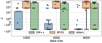
Figure 2: Box plot and raw data of NLL $\mathcal{L}$ (9) using estimated parameters. The box draws from the first quartile $Q_{1}$ to the third quartile $Q_{3}$. Whiskers extend up to $1.5$ times the interquartile range $\mathrm{IQR}=Q_{3}-Q_{1}$ from $Q_{1}$ and $Q_{3}$. The median of each category is indicated by a red line. The individual value of NLL $\mathcal{L}$ for each method are shown as dots.

Although individual iterations of EM++ are slower, due to solving an internal optimization problem in Python, it requires significantly fewer iterations, especially for larger training datasets. In contrast, both BFGS and Adam need more iterations as the dataset size increases. Despite fast individual iterations, the overall process of both algorithms becomes less efficient when given larger dataset. The effectiveness of the EM++ method is further demonstrated by its convergence to points with lower loss, as evidenced in Fig. 2. The NLL $\mathcal{L}$ improves with larger training datasets, whereas both BFGS and Adam do not significantly benefit from the additional data.

6.2 Comparison with tailored algorithms

We compare EM++ against tailored algorithms [9, 8] for different switching systems, using 3 formulations for (1a): 1 only-mode: $\bm{\Theta}\mapsto\sigma\big{(}\begin{bmatrix}\Theta_{i}&0\end{bmatrix}^{\top}\big{)}$; 2 only-state: $\bm{\Theta}\mapsto\sigma\big{(}\begin{bmatrix}z^{\top}\Theta&0\end{bmatrix}^{\top}\big{)}$ where $\Theta_{i}=\Theta$; and 3 full-dependence: $\bm{\Theta}\mapsto\sigma\big{(}\begin{bmatrix}z^{\top}\Theta_{i}&0\end{bmatrix}^{\top}\big{)}$, for all $i\in\Xi$. To assess the flexibility of (1b) in a robust identification scenario, we consider both the Gaussian distribution and the Student’s t-distribution, a common choice in robust system identification. Unless otherwise specified, each algorithm is trained with 5 initial guesses, with hyperparameters tuned by hold-out validation. The best solution on a separate validation data set is selected to compare prediction accuracy. For trajectory prediction initialization, both framework [9] and our options only-mode, full-dependence use training and validation set. The latter two options use (32) to compute initial mode distribution. Denoting the ground truth with $y_{n}$ and the prediction with $\hat{y}_{n}$, the prediction accuracy is measured by the $R^{2}$ score:

$$R^{2}=1-\frac{\sum_{n=1}^{N}\left(y_{n}-\hat{y}_{n}\right)^{2}}{\sum_{n=1}^{N}\left(y_{n}-\tfrac{1}{N}\sum_{n=1}^{N}y_{n}\right)^{2}}.$$

6.2.1 Switched Markov ARX system

Table 3: $R^{2}$ score of recursive one-step-ahead prediction for switched Markov ARX system (38) ($\uparrow$)

		EM++ (Gaussian distribution)		EM++ (Student’s t-distribution)
	framework [9]	only-mode	full-dependence	only-mode	full-dependence
$p=0$	0.9286	0.9526	0.9540	0.9536	$\bm{0.9548}$
$p=0.01$	0.9452	0.9341	0.9357	0.9528	$\bm{0.9560}$
$p=0.05$	0.9367	0.8521	0.7623	0.8810	$\bm{0.9477}$

We collect a trajectory with $T=10000$ data points from a switching Markov ARX system:

$$y_{t}=\beta_{\xi_{t}}^{\top}z_{t-1}+w_{t},$$ (38)

where $z_{t-1}=\begin{bmatrix}y_{t-1}&y_{t-2}&u_{t-1}&u_{t-2}\end{bmatrix}^{\top}$. It consists of three subsystems with parameters $\beta_{1}^{\top}=\begin{bmatrix}1.143&-0.4346&0.0572&0.2415\end{bmatrix}$, $\beta_{2}^{\top}=\begin{bmatrix}0.9534&-0.0475&0.0618&0.0336\end{bmatrix}$, $\beta_{3}^{\top}=\begin{bmatrix}1.178&-0.09&0.089&0.15\end{bmatrix}$, and additive noise $w_{t}\sim\mathcal{N}(0,0.025)$. Switching occurs according to a transition matrix $P=\begin{bmatrix}0.25&0.1&0.65\\ 0.55&0.35&0.1\\ 0.15&0.15&0.7\\ \end{bmatrix}.$ The control input is randomly sampled in $[-1,1]$. The 10000 data points are split into a training (5000), validation (2500), and test (2500) set. Each training data point has probability $p\in\{0\%,1\%,5\%\}$ of being perturbed by noise sampled from $[-\max_{t}\left\lvert y_{t}\right\rvert,\max_{t}\left\lvert y_{t}\right\rvert]$. EM++ is compared to the framework [9]. The solutions are evaluated using the recursive one-step ahead prediction: at each time step $t$, the algorithm predicts one-step ahead, then is updated by the true observation $y_{t}$ [9, algorithm 3]. For our stochastic model, we compute the mean over 20 trajectory samples for evaluation. The result is in Table 3. As $f$ for the Student’s t-distribution is a nonlinear function (cf. Table 1), constructing the surrogate function (16d) requires evaluating the linearization of $f$. In contrast, the Gaussian distribution does not necessitate this step as its $f$ is linear (cf. Table 1). To evaluate the impact of this additional majorization step via linearization, we in addition compare the performance of the algorithm with those two noise options. The progress plot for both options with the same initial guess is illustrated in Fig. 3.

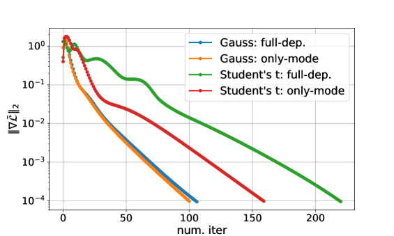
Figure 3: Gradient norm evaluation for Markov jump ARX system (38) with different noise and switching options.

EM++ with the Student’s t-distribution model demonstrates superior performance compared to the framework [9], despite requiring more iterations. The increased iteration count owes to the necessity of computing a linearization (16d) for the Student’s t distribution, which results in a looser approximation of the original loss. However, this trade-off is justified by its robustness to outliers. While the model with the Gaussian distribution achieves high $R^{2}$ score without outliers, the scores drop significantly as the proportion of outliers increases, since the Gaussian parameter estimation is sensitive to outliers. This comparison highlights the necessity of a subsystem model tailored to the specific problem. Comparing the full-dependence and only-mode options, we observe that the former requirs more iterations due to its increased number of variables. Nevertheless, the model with option full-dependence reaches a similar score as the model utilizing the prior knowledge on the switching (only-mode) in most cases. This suggests that the proposed method is able to learn the system’s intrinsic structure without prior knowledge.

6.2.2 Piecewise affine system

We collect a trajectory with $T=10000$ data points from a piecewise affine system:

$$\begin{cases}y_{t}=\beta_{1}^{\top}z_{t-1}+w_{t}&\text{if}\quad\beta_{0}^{\top}z_{t-1}\geq 0,\\ y_{t}=\beta_{2}^{\top}z_{t-1}+w_{t}&\text{otherwise},\end{cases}$$ (39)

where $z_{t-1}=\begin{bmatrix}y_{t-1}&y_{t-2}&u_{t-1}&u_{t-2}&1\end{bmatrix}^{\top}$. The system parameters are $\beta_{0}^{\top}=\begin{bmatrix}0.5&1&2&-0.3&0.2\end{bmatrix}$, $\beta_{1}^{\top}=\begin{bmatrix}0.1&0.5&-0.4&0.3&0\end{bmatrix}$, $\beta_{2}^{\top}=\begin{bmatrix}0.2&0.4&0.1&0.4&0\end{bmatrix}$, and the system is subject to an additive noise $w_{t}\sim\mathcal{N}(0,10^{-4})$. The control input is randomly sampled from $\mathcal{N}(0,0.25)$. The data are split as in Section 6.2.1. EM++ is compared with the framework [9], and a tailored algorithm for piecewise affine models, PARC [8]. The identified models are evaluated using the open-loop prediction with the same control input that generates the test dataset. For our stochastic model (1), we employ $1\%$ trimmed mean of 500 sampled trajectories as the prediction, since the trimmed mean is less sensitive to rare events. The $R^{2}$ score is listed in Table 4. Same as Section 6.2.1, we compare the performance of the algorithm using both Gaussian and Student’s t-distribution. This comparison evaluates the impact of the additional majorization step described in Proposition 3.2. The progress plot for both options with the same initial guess is in Fig. 4.

Table 4: $R^{2}$ score of open-loop prediction for piecewise affine system (39) ($\uparrow$)

			EM++ (Gaussian distribution)		EM++ (Student’s t-distribution)
	framework [9]	PARC [8]	only-state	full-dependence	only-state	full-dependence
$p=0$	0.8569	0.9883	0.9905	$\bm{0.9909}$	0.9904	0.9905
$p=0.01$	0.8601	0.9764	0.9537	0.9572	0.9901	$\bm{0.9903}$
$p=0.05$	0.8428	0.9050	0.8600	0.8689	$\bm{0.9881}$	$\bm{0.9881}$

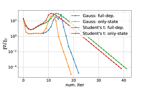
Figure 4: Gradient norm evaluation for piecewise affine system (39) with different noise and switching options.

Both PARC and EM++ outperform the framework [9]. The enhanced performance can be attributed to the robustness against subsystem estimation error achieved by softmax modelling in (1a), compared to a Voronoi-distance-based method used by the framework [9]. As the number of outliers increases, the performance of both PARC and of the proposed models with a Gaussian distribution decreases significantly. In contrast, the models with the Student’s t-distribution maintain high prediction accuracy, despite a slight increase in the number of iterations due to the additional majorization step via linearization (16d). We observe that option full-dependence requires more iterations than option only-state due to its increased number of variables. Nevertheless, it achieves a similar $R^{2}$ score as the option only-state, akin to the previous example. This suggests that our proposed method is able to learn the system’s intrinsic structure without prior information. This ability is particularly beneficial when (accurate) prior information is unavailable.

6.2.3 Cart system

We further compare EM++ with PARC [8] on a cart system [8] that is piecewise nonlinear:

$$\left\{\begin{aligned} \dot{p}&=\tfrac{1}{M+M_{1}}\left(F-\varphi_{b}(\dot{p},b_{1}+b)-\varphi_{a}(p-a-\alpha_{1},k_{1})\right)\\ \dot{T}&=\tfrac{1}{\Theta}\left(\tfrac{T_{0}-T}{R}+\tfrac{T_{1}-T}{R_{1}}\right),\quad\text{if }p-a\leq\alpha_{1}\end{aligned}\right.$$

$$\left\{\begin{aligned} \dot{p}&=\tfrac{1}{M+M_{2}}\left(F-\varphi_{b}(\dot{p},b_{2}+b)-\varphi_{a}(p+a-\alpha_{2},k_{2})\right)\\ \dot{T}&=\tfrac{1}{\Theta}\left(\tfrac{T_{0}-T}{R}+\tfrac{T_{2}-T}{R_{2}}\right),\quad\text{if }p+a\geq\alpha_{2}\end{aligned}\right.$$

$$\left\{\begin{aligned} \dot{p}&=\tfrac{1}{M}\left(F-\varphi_{b}(\dot{p},b)\right)\\ \dot{T}&=\tfrac{T_{0}-T}{\Theta R},\quad\text{otherwise}\end{aligned}\right.$$ (40)

where $\varphi_{a}(\Delta p,k)=k\Delta p+\frac{k}{5}\Delta p^{3},\varphi_{b}(\dot{p},b)=b\dot{p}+\frac{b}{5}|\dot{p}|\dot{p}.$ The cart is controlled by a switching command $u\in\{-1,0,1\}$ that is generated every $T_{s}=$0.5\text{\,}\mathrm{s}$$ according to a transition matrix: $P=\begin{bmatrix}\frac{29}{30}&\frac{1}{60}&\frac{1}{60}\\ \frac{1}{60}&\frac{29}{30}&\frac{1}{60}\\ \frac{1}{60}&\frac{1}{60}&\frac{29}{30}\\ \end{bmatrix}.$ The control input determines $F=u$. The other parameters can be found in [8, TABLE VIII]. We collect $4000$ training data points and $550$ validation data points initialized at $x_{0}=\begin{bmatrix}p&\dot{p}&T\end{bmatrix}=\begin{bmatrix}2&0&25+273.15\end{bmatrix}$, and $530$ testing data points initialized at $\begin{bmatrix}p&\dot{p}&T\end{bmatrix}=\begin{bmatrix}1.5&0&40+273.15\end{bmatrix}$. We use the state-input pair $z_{t}=\begin{bmatrix}x_{t}^{\top}&u_{t}&1\end{bmatrix}^{\top}$ as input and produce $x_{t+1}$ as output. To ensure that all state variables are of the same order of magnitude, we convert the temperature $T$ into Celsius and divide it by $10$. PARC is initialized with K-means++ and with same hyperparameters as in [8], while EM++ uses random initialization. The identified models are evaluated using the open-loop prediction on the last $500$ data points of the testing dataset, using the same control input that generates the test data. For option full-dependence, we estimate the initial mode distribution using the first $30$ points of testing dataset via (32). For our stochastic model (1), we employ $1\%$ trimmed mean of 500 sampled trajectories as the prediction, since the trimmed mean is less sensitive to rare events. The $R^{2}$ score for each method is summarized in Table 5.

Table 5: $R^{2}$ of open-loop prediction for cart system (40) ($\uparrow$)

$d$	method name	$R^{2}(p)$	$R^{2}(\dot{p})$	$R^{2}(T)$
3	PARC [8]	${0.927}$	${0.900}$	$\bm{0.920}$
	EM++ (only-state)	$\bm{0.931}$	$\bm{0.909}$	0.912
	EM++ (full-dependence)	0.917	0.901	0.877
5	PARC [8]	$0.948$	${0.930}$	$0.935$
	EM++ (only-state)	0.948	$\bm{0.935}$	0.928
	EM++ (full-dependence)	$\bm{0.972}$	0.931	$\bm{0.976}$
7	PARC [8]	$\bm{0.982}$	$0.967$	$\bm{0.978}$
	EM++ (only-state)	0.959	0.947	0.946
	EM++ (full-dependence)	0.978	$\bm{0.971}$	0.966

From Table 5, we observe that EM++ achieves comparable $R^{2}$ to the tailored algorithm [8]. When the number of modes $d$ matches the underlying true model, the case only-state exhibits higher prediction accuracy, as the model aligns with the underlying switching mechanism. However, by increasing the number of modes, the case full-dependence has more flexibility to capture the underlying nonlinearity in the cart system (40), resulting in higher $R^{2}$ score.

6.3 Case study: Coupled electric drives

This section examines the expressiveness of our proposed method through a coupled electric drives system dataset [50]. The system employs two electric motors to drive a pulley via a flexible belt. The pulley is supported by a spring, resulting in lightly damped dynamics. The system measures the absolute angular velocity of the pulley using a direction-insensitive sensor. The dataset consists of two trajectories, each containing 500 data points sampled in 50 Hz. The data points in each trajectory are allocated into training (300), validation (100), and testing (100) sets. We choose the mode number $d=8$ and use ARX form with $z_{t-1}=\begin{bmatrix}y_{t-1}&\dots&y_{t-3}&u_{t-1}&\dots&u_{t-3}&1\end{bmatrix}^{\top}$. This switching ARX model is compared against different types of ARX models listed in Table 6. In particular, the neural network ARX (NN-ARX) consists of two hidden layers, each with $32$ neurons. We use one layer of LSTM with hidden size equals to $32$. The number of modes in PARC is $8$, same as for our model. All models use the same lag value with hyperparameters grid-searched on the validation set. Each model is trained for 20 times with different random initial guesses. The best parameters on the validation set are chosen for comparison, which evaluates the open-loop simulation error of each identified model. For simulation initialization, both LSTM and model (1) use the training and validation set. The latter uses (32) to compute the initial mode distribution. Same as [7], we use root-mean-square error (RMSE) as comparison metric: $\mathrm{RMSE}=\sqrt{\frac{1}{N}\sum_{n=1}^{N}\left(y_{n}-\hat{y}_{n}\right)^{2}}$ where $y_{n}$ is the ground truth trajectory and $\hat{y}_{n}$ denotes the open-loop prediction. As both our model (1) and Gaussian Process (GP)-ARX are stochastic models that outputs a trajectory distribution, we sample 500 trajectories from each identified distribution. We compute the $1\%$ trimmed mean of the sampled trajectories as the prediction for the $\mathrm{RMSE}$, which is less sensitive to rare events. The open-loop prediction of identified proposed model in shown in Fig. 5. The RMSE of all methods is summarized in Table 6.

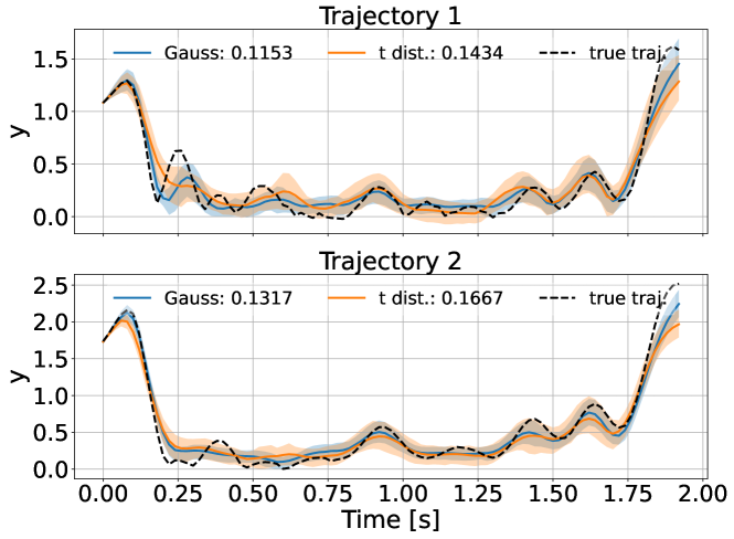
Figure 5: Open-loop prediction for coupled electric drives. Colored area shows quantiles between $0.25$ and $0.75$.

Table 6: RMSE of open-loop prediction ($\downarrow$) (The best three results are in bold, bold and italic, and italic font, respectively.)

method	RMSE
	traj. 1	traj. 2
ARX	0.196	0.344
GP-ARX (with rbf)	0.143	0.207
GP-ARX (with Matern32)	0.149	0.204
NN-ARX (with ReLU)	0.212	0.214
NN-ARX (with SiLU)	0.161	0.179
LSTM	0.104	0.121
PARC [8]	0.178	0.216
DT subspace encoder[7]	0.130	0.145
CT subspace encoder ($\Delta t=0.03$)[7]	0.085	0.072
EM++ (Gaussian distribution)	0.115	0.132
EM++ (Student’s t-distribution)	0.143	0.167

As shown in Table 6, our method achieves better prediction accuracy compared to GP-ARX, NN-ARX, and PARC. This superior performance demonstrates the expressiveness of the proposed model. The enhanced result of CT subspace encoder may attribute to its continuous-time modelling approach. However, our method is comparable to its discrete-time variant (DT subspace encoder) and LSTM, with the added benefits of a simpler structure and improved interpretability. This maintains the model’s expressive power while ensuring an easier understanding and analysis.

7 Conclusion

This work presented a general switching system model that encompasses various popular models. Additionally, we proposed an algorithm EM++ (cf. Algorithm 1) to identify the parameters of this generic model by solving a regularized maximum likelihood estimation problem. We proved that EM++ converges to stationary points under suitable assumptions. Finally, the effectiveness of both the presented model and the algorithm was demonstrated in a series of numerical experiments. Future work includes: generalizing the model with continuous latent variables; adapting EM++ for online use; and integrating the model into a model-based control framework such as model predictive control.

References

• [1] Aleksandr Aravkin, James V Burke, Lennart Ljung, Aurelie Lozano, and Gianluigi Pillonetto. Generalized kalman smoothing: Modeling and algorithms. Automatica, 86:63–86, 2017.
• [2] Aleksandr Y Aravkin, Bradley M Bell, James V Burke, and Gianluigi Pillonetto. An $\ell_{1}$-laplace robust kalman smoother. IEEE Transactions on Automatic Control, 56(12):2898–2911, 2011.
• [3] Hédy Attouch, Jérôme Bolte, Patrick Redont, and Antoine Soubeyran. Proximal alternating minimization and projection methods for nonconvex problems: An approach based on the kurdyka-Łojasiewicz inequality. Mathematics of Operations Research, 35(2):438–457, 2010.
• [4] Heinz H. Bauschke, Jérôme Bolte, and Marc Teboulle. A descent lemma beyond lipschitz gradient continuity: First-order methods revisited and applications. 42(2):330–348. Publisher: INFORMS.
• [5] Heinz H Bauschke, Jonathan M Borwein, et al. Legendre functions and the method of random bregman projections. Journal of convex analysis, 4(1):27–67, 1997.
• [6] Amir Beck and Marc Teboulle. Mirror descent and nonlinear projected subgradient methods for convex optimization. Operations Research Letters, 31(3):167–175, 2003.
• [7] Gerben I. Beintema, Maarten Schoukens, and Roland Tóth. Continuous-time identification of dynamic state-space models by deep subspace encoding. In The Eleventh International Conference on Learning Representations, 2023.
• [8] Alberto Bemporad. A piecewise linear regression and classification algorithm with application to learning and model predictive control of hybrid systems. IEEE Transactions on Automatic Control, 2022.
• [9] Alberto Bemporad, Valentina Breschi, Dario Piga, and Stephen P Boyd. Fitting jump models. Automatica, 96:11–21, 2018.
• [10] Federico Bianchi, Alessandro Falsone, Luigi Piroddi, and Maria Prandini. An alternating optimization method for switched linear systems identification. IFAC-PapersOnLine, 53(2):1071–1076, 2020.
• [11] Christopher M Bishop. Pattern recognition and machine learning, volume 4. Springer, 2006.
• [12] Jérôme Bolte, Aris Daniilidis, and Adrian Lewis. The łojasiewicz inequality for nonsmooth subanalytic functions with applications to subgradient dynamical systems. SIAM Journal on Optimization, 17(4):1205–1223, 2007.
• [13] Jérôme Bolte, Shoham Sabach, Marc Teboulle, and Yakov Vaisbourd. First order methods beyond convexity and lipschitz gradient continuity with applications to quadratic inverse problems. SIAM Journal on Optimization, 28(3):2131–2151, 2018.
• [14] Lev M Bregman. The relaxation method of finding the common point of convex sets and its application to the solution of problems in convex programming. USSR computational mathematics and mathematical physics, 7(3):200–217, 1967.
• [15] Valentina Breschi, Dario Piga, and Alberto Bemporad. Piecewise affine regression via recursive multiple least squares and multicategory discrimination. Automatica, 73:155–162, 2016.
• [16] Stéphane Chrétien and Alfred O Hero. On em algorithms and their proximal generalizations. ESAIM: Probability and Statistics, 12:308–326, 2008.
• [17] Oswaldo Luiz Valle Costa, Marcelo Dutra Fragoso, and Ricardo Paulino Marques. Discrete-time Markov jump linear systems. Springer Science & Business Media, 2005.
• [18] Yingwei Du, Fangzhou Liu, Jianbin Qiu, and Martin Buss. Online identification of piecewise affine systems using integral concurrent learning. IEEE Transactions on Circuits and Systems I: Regular Papers, 68(10):4324–4336, 2021.
• [19] Bradley Efron. Exponential families in theory and practice. Cambridge University Press, 2022.
• [20] Francisco Facchinei and Jong-Shi Pang. Finite-dimensional variational inequalities and complementarity problems. Springer, 2003.
• [21] Lei Fan, Hariprasad Kodamana, and Biao Huang. Robust identification of switching markov arx models using em algorithm. IFAC-PapersOnLine, 50(1):9772–9777, 2017.
• [22] David R Hunter and Kenneth Lange. A tutorial on mm algorithms. The American Statistician, 58(1):30–37, 2004.
• [23] X Jin and Biao Huang. Identification of switched markov autoregressive exogenous systems with hidden switching state. Automatica, 48(2):436–441, 2012.
• [24] Norman L Johnson, Samuel Kotz, and Narayanaswamy Balakrishnan. Continuous univariate distributions, volume 2, volume 289. John wiley & sons, 1995.
• [25] Michael I Jordan and Robert A Jacobs. Hierarchical mixtures of experts and the em algorithm. Neural computation, 6(2):181–214, 1994.
• [26] Diederik P Kingma and Jimmy Ba. Adam: A method for stochastic optimization. arXiv preprint arXiv:1412.6980, 2014.
• [27] Hariprasad Kodamana, Biao Huang, Rishik Ranjan, Yujia Zhao, Ruomu Tan, and Nima Sammaknejad. Approaches to robust process identification: A review and tutorial of probabilistic methods. Journal of Process Control, 66:68–83, 2018.
• [28] Oliver Kroemer, Herke Van Hoof, Gerhard Neumann, and Jan Peters. Learning to predict phases of manipulation tasks as hidden states. In 2014 IEEE International Conference on Robotics and Automation, pages 4009–4014. IEEE, 2014.
• [29] Frederik Kunstner, Raunak Kumar, and Mark Schmidt. Homeomorphic-invariance of em: Non-asymptotic convergence in kl divergence for exponential families via mirror descent. In International Conference on Artificial Intelligence and Statistics, pages 3295–3303. PMLR, 2021.
• [30] Kenneth Lange. MM optimization algorithms. SIAM, 2016.
• [31] Yann LeCun, Sumit Chopra, Raia Hadsell, M Ranzato, and Fujie Huang. A tutorial on energy-based learning. Predicting structured data, 1(0), 2006.
• [32] Jessica Leoni, Valentina Breschi, Simone Formentin, and Mara Tanelli. Explainable data-driven modelling via mixture of experts: towards effective blending of grey and black-box models. arXiv preprint arXiv:2401.17118, 2024.
• [33] Xinpeng Liu and Xianqiang Yang. A variational bayesian approach for robust identification of linear parameter varying systems using mixture laplace distributions. Neurocomputing, 395:15–23, 2020.
• [34] Stanislaw Lojasiewicz. Une propriété topologique des sous-ensembles analytiques réels. Les équations aux dérivées partielles, 117:87–89, 1963.
• [35] Haihao Lu, Robert M. Freund, and Yurii Nesterov. Relatively smooth convex optimization by first-order methods, and applications. SIAM Journal on Optimization, 28(1):333–354, 2018.
• [36] Ali Moradvandi, Ralph EF Lindeboom, Edo Abraham, and Bart De Schutter. Models and methods for hybrid system identification: a systematic survey. IFAC-PapersOnLine, 56(2):95–107, 2023.
• [37] Jorge Nocedal and Stephen J Wright. Numerical optimization. Springer, 1999.
• [38] Simone Paoletti, Aleksandar Lj Juloski, Giancarlo Ferrari-Trecate, and René Vidal. Identification of hybrid systems a tutorial. European journal of control, 13(2-3):242–260, 2007.
• [39] Adam Paszke, Sam Gross, Francisco Massa, Adam Lerer, James Bradbury, Gregory Chanan, and et al. Pytorch: An imperative style, high-performance deep learning library. In Advances in Neural Information Processing Systems 32, pages 8024–8035. Curran Associates, Inc., 2019.
• [40] Lawrence R Rabiner. A tutorial on hidden markov models and selected applications in speech recognition. Proceedings of the IEEE, 77(2):257–286, 1989.
• [41] Meisam Razaviyayn, Mingyi Hong, and Zhi-Quan Luo. A unified convergence analysis of block successive minimization methods for nonsmooth optimization. SIAM Journal on Optimization, 23(2):1126–1153, 2013.
• [42] R Tyrrell Rockafellar. Convex analysis, volume 11. Princeton university press, 1997.
• [43] R. Tyrrell Rockafellar and Roger J. B. Wets. Variational Analysis, volume 317 of Grundlehren Der Mathematischen Wissenschaften. Springer Berlin Heidelberg, Berlin, Heidelberg, 1998.
• [44] Michael Roth. On the multivariate t distribution. Linköping University Electronic Press, 2012.
• [45] Nima Sammaknejad, Yujia Zhao, and Biao Huang. A review of the expectation maximization algorithm in data-driven process identification. Journal of process control, 73:123–136, 2019.
• [46] Ying Sun, Prabhu Babu, and Daniel P Palomar. Majorization-minimization algorithms in signal processing, communications, and machine learning. IEEE Transactions on Signal Processing, 65(3):794–816, 2016.
• [47] Paul Tseng. An analysis of the em algorithm and entropy-like proximal point methods. Mathematics of Operations Research, 29(1):27–44, 2004.
• [48] Pauli Virtanen, Ralf Gommers, Travis E. Oliphant, Matt Haberland, Tyler Reddy, David Cournapeau, and et al. SciPy 1.0: Fundamental Algorithms for Scientific Computing in Python. Nature Methods, 17:261–272, 2020.
• [49] Martin J Wainwright, Michael I Jordan, et al. Graphical models, exponential families, and variational inference. Foundations and Trends® in Machine Learning, 1(1–2):1–305, 2008.
• [50] T. Wigren and M. Schoukens. Coupled electric drives data set and reference models. Technical report, Department of Information Technology, Uppsala University, 2017.
• [51] CF Jeff Wu. On the convergence properties of the em algorithm. The Annals of statistics, pages 95–103, 1983.