SOAP: Enhancing Spatio-Temporal Relation and Motion
Information Capturing for Few-Shot Action Recognition

Abstract.

High frame-rate (HFR) videos of action recognition improve fine-grained expression while reducing the spatio-temporal relation and motion information density. Thus, large amounts of video samples are continuously required for traditional data-driven training. However, samples are not always sufficient in real-world scenarios, promoting few-shot action recognition (FSAR) research. We observe that most recent FSAR works build spatio-temporal relation of video samples via temporal alignment after spatial feature extraction, cutting apart spatial and temporal features within samples. They also capture motion information via narrow perspectives between adjacent frames without considering density, leading to insufficient motion information capturing. Therefore, we propose a novel plug-and-play architecture for FSAR called $\underline{\textbf{S}}$patio-temp$\underline{\textbf{O}}$ral fr$\underline{\textbf{A}}$me tu$\underline{\textbf{P}}$le enhancer (SOAP) in this paper. The model we designed with such architecture refers to SOAP-Net. Temporal connections between different feature channels and spatio-temporal relation of features are considered instead of simple feature extraction. Comprehensive motion information is also captured, using frame tuples with multiple frames containing more motion information than adjacent frames. Combining frame tuples of diverse frame counts further provides a broader perspective. SOAP-Net achieves new state-of-the-art performance across well-known benchmarks such as SthSthV2, Kinetics, UCF101, and HMDB51. Extensive empirical evaluations underscore the competitiveness, pluggability, generalization, and robustness of SOAP. The code is released at https://github.com/wenbohuang1002/SOAP.

1. Introduction

\begin{overpic}[width=208.13574pt]{figures/fluency_R.pdf} \put(1.5,37.0){\footnotesize\color[rgb]{1,0,0}{HFR}} \put(1.5,24.0){\footnotesize\color[rgb]{0,0,1}{LFR}} \put(18.0,50.0){{?}} \put(34.0,52.0){\footnotesize Subtle Timeline \& Displacement} \put(34.0,48.0){\footnotesize\color[rgb]{1,0,0}{Weak Spatio-temporal Realtion}} \put(34.0,44.0){\footnotesize\color[rgb]{1,0,0}{Low Motion Information Density}} \put(34.0,17.0){\footnotesize Clear Timeline \& Displacement} \put(34.0,13.0){\footnotesize\color[rgb]{0,0,1}{Strong Spatio-temporal Realtion}} \put(34.0,9.0){\footnotesize\color[rgb]{0,0,1}{High Motion Information Density}} \put(52.0,58.0){\footnotesize More Video Samples} \put(52.0,3.0){\footnotesize Fewer Video Samples} \put(82.0,22.0){\footnotesize Data-driven} \put(84.0,18.0){\footnotesize Training} \end{overpic}

Figure 1. Spatio-temporal relation and motion information density of HFR video frames are much subtler, reflecting by timeline and displacement. Therefore, larger amounts of samples are required for data-driven training.

Ubiquitous videos in daily lives are rapidly accelerating the development of multimedia analytic research. As a fundamental task, action recognition is experiencing an explosive demand in a wide range of applications including intelligent surveillance, video understanding, and health monitoring (Liu and Ma, 2019; Reddy et al., 2022; Croitoru et al., 2021). Progress in video recorders contributes to high frame-rate (HFR) videos, with more similar frames per second improving the expression of fine-grained actions (Pan et al., 2023). As the example shown in Figure 1, we can explicitly observe that the timeline and displacement of object in HFR video frames are much subtler than those in low frame-rate (LFR) video frames, better reflecting fine-grained actions. However, the spatio-temporal relation and motion information density decrease with the improvement of video fluency (Ye et al., 2021). Therefore, a larger amount of video samples are continuously required to train data-driven models. Unfortunately, samples for target actions such as “falling down” are usually insufficient and hard to collect in real-world scenarios. Contemporary few-shot learning mitigates data dependence by transferring knowledge from a few samples, promoting few-shot action recognition (FSAR) research.
According to data characteristics of HFR videos, two prevailing challenges of FSAR exist. Challenge 1: Optimizing spatio-temporal relation construction. Spatial and temporal features work as a whole in video samples, only focusing on spatial information makes models misidentify horizontal or vertical actions such as “pushing”, “pulling”, “putting up”, and “putting down”. However, the spatio-temporal relation of HFR videos is subtle, making the construction challenging. Challenge 2: Comprehensive motion information capturing. As an exclusive characteristic of videos, motion information plays a crucial role in helping models recognize target actions in a dynamic manner. However, the difficulties in motion information capturing is exaggerated by low motion information density from HFR videos and limited frames processed at one time with mainstream methods. In summary, the challenges mentioned above not only stem from HFR videos but are also aggravated by the insufficient samples in few-shot settings.
In FSAR, the metric-based paradigm predominates due to its simplicity and efficacy. It embeds samples into action prototypes to calculate support-query distances for classification in an episodic task (Zhu and Yang, 2018; Cao et al., 2020; Perrett et al., 2021; Wang et al., 2022; Zhang et al., 2023). We observe that these works prioritize temporal alignment after spatial feature extraction, cutting apart spatial and temporal features within samples and overlooking the importance of motion information capture. Some works (Wang et al., 2023b; Wu et al., 2022; Wanyan et al., 2023) incorporate motion information into action recognition and achieve remarkable performance. However, the motion information is captured between adjacent frames. This narrow perspective inevitably overlooks density of motion information and results in inadequate capturing. So far, no solution exists for both challenges.
Motivated by aforementioned challenges, we propose a novel plug-and-play architecture for FSAR called $\underline{\textbf{S}}$patio-temp$\underline{\textbf{O}}$ral fr$\underline{\textbf{A}}$me tu$\underline{\textbf{P}}$le enhancer (SOAP). The model we designed with such architecture is defined as SOAP-Net. The cores are optimizing construction of spatio-temporal relation and capturing comprehensive motion information. For the first goal, simply extracting features from video frames is insufficient. These features are located in different channels and have temporal connections between each channel. Spatio-temporal relation within features also play a key role in FSAR. For the second goal, we consider motion information density and find that frame tuples with multiple frames contain richer motion information than adjacent frames. Combining frame tuples of various frame counts further provides a broader perspective. To be specific, SOAP has three components: 3-Dimension Enhancement Module (3DEM) uses a 3D convolution for spatio-temporal relation construction and Channel-Wise Enhancement Module (CWEM) calibrates channel-wise feature responses adaptively while Hybrid Motion Enhancement Module (HMEM) applies a broader perspective to help models capture comprehensive motion information. These three modules work in parallel, adding priors into raw input.
To our best knowledge, SOAP is the first to address all challenges simultaneously. Our main contribution are three-fold:

• Spatio-Temporal Relation Construction. The proposed SOAP optimizes spatio-temporal relation construction, avoiding simply operating temporal alignment after extracting spatial features.

• Motion Information Capturing. Taking motion information density and the processing method into account, our SOAP finds a comprehensive solution, overcoming the second challenge with a broader perspective that combines frame tuples with various frame counts.

• Effectiveness. SOAP-Net achieves new SOTA performance on several well-known FSAR benchmarks, including SthSthV2, Kinetics, UCF101, and HMDB51. Comprehensive experiments demonstrate the competitiveness, pluggability, generalization, and robustness of SOAP.

2. Related Works

2.1. Few-Shot Learning

The core goal of few-shot learning is to recognize unseen classes from only few samples. Unlike traditional deep learning, few-shot learning utilizes episodic training where training units are structured as similar tasks with small labeled sets. Three primary groups of few-shot learning are data-augmentation based, optimization-based, and metric-based paradigms. In the first data-augmentation paradigm, generating additional samples to supplement available data is a key feature. Specifically, MetaGAN (Zhang et al., 2018) utilizes generative adversarial networks (GANs) and statistics of existing samples to synthesize data. The most representative optimization-based method is MAML (Finn et al., 2017), which identifies a model parameters set and adapts it to individual tasks via gradient descent. The metric-based paradigm is well-known and widely used for its simplicity and effectiveness. It leverages similarity between support samples to classify query samples into corresponding classes. Prototypical Networks (Snell et al., 2017) construct prototypes based on class centroids and then classify samples by measuring distance to each prototype. Most few-shot learning paradigms are applied to image classification, with fewer in the field of videos. Our SOAP belongs to the metric-based paradigm for FSAR, focusing on improving prototype representation ability.

2.2. Action Recognition

Compared to image classification, action recognition is a more complex and extensively researched problem in the community due to the spatio-temporal relation and motion information. Previous works (Piergiovanni and Ryoo, 2019; Wang et al., 2021; Chen et al., 2021; Wasim et al., 2023) have typically utilized 3D backbones to construct spatio-temporal relations, while optical flow is applied by additional networks to inject video motion information for action recognition, resulting in promising results. However, these works with high acquisition costs are all designed for traditional data-driven training without considering insufficient samples in real-world scenarios. In contrast, SOAP is specifically designed for a more realistic few-shot setting.

2.3. Few-Shot Action Recognition

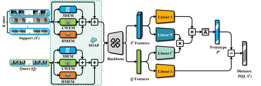
Figure 2. Overview of the SOAP-Net. It comprises three main modules: the 3DEM for constructing relation between spatial and temporal information, the CWEM for modeling temporal connections between channels, and the HMEM for capturing comprehensive motion information with frame tuples of varying frame counts using a hybrid approach. The “$\bar{\textbf{A}}$” symbol at the right part of the figure shows an averaging calculation used to construct a query-specific prototype $P^{c}$ in Eqn (17).

Existing methods of FSAR mainly focus on metric-based paradigm for effective prototype construction. Among them, CMN (Zhu and Yang, 2018, 2020) introduces a multi-saliency embedding algorithm for key frame encoding, improving the prototype representation; ARN (Zhang et al., 2020) captures short-range dependencies using 3D backbones with a self-trained permutation invariant attention; OTAM (Cao et al., 2020) aligns support and query with a dynamic time warping (DTW) algorithm. Joint spatio-temporal modeling approaches such as TA²N (Li et al., 2022), ITA (Zhang et al., 2021), STRM (Thatipelli et al., 2022), and SloshNet (Xing et al., 2023a) employ spatial-temporal frameworks to address the support-query misalignment from multiple perspectives; Temporal relation is emphasized by TRX (Perrett et al., 2021), using a Cross Transformer for sub-sequence alignment and achieving notable improvement; HyRSM (Wang et al., 2022) learns the task-specific embedding by exploiting the relation within and cross videos; SA-CT (Zhang et al., 2023) complement the temporal information by learning the spatial relation. The temporal alignment all operated after spatial feature extraction. Diverse types of information including optical flow (Wanyan et al., 2023) and depth (Fu et al., 2020) are introduced by extra networks, increasing computations. MoLo (Wang et al., 2023b) and MTFAN (Wu et al., 2022) explicitly extract motion information from raw videos and leverage temporal context for FSAR. Although achieving promising performance, these works are either cut apart spatial and temporal features or ignore motion information density. Therefore, our SOAP focuses on spatio-temporal relation and motion information capturing.

3. Methodology

3.1. Problem Formulation

Classifying an unlabeled query into one of the support classes is the inference goal of FSAR. The support set has at least one labeled sample per class. Following the prior works (Cao et al., 2020; Perrett et al., 2021; Wang et al., 2022, 2023b), we randomly select few-shot tasks from training set for episodic training. In each task, the support set $S$ contains $N$ classes and $K$ samples per class, i.e., $N$-way $K$-shot setting. The query set $Q$ in each task has samples to be classified. Uniformly sampling $F$ frames of each video, we define the $k^{\text{th}}\left(k=1,\cdots,K\right)$ sample of the $c^{\text{th}}\left(c=1,\cdots,N\right)$ class of support set $S$ as:

(1) $$S^{ck}=\left[s_{1}^{ck},\dots,s_{F}^{ck}\right]\in\mathbb{R}^{F\times C\times H\times W}.$$

Notions used are $F$ (frames), $C$ (channels), $H$ (height), and $W$ (width), while the sample with $F$ frames of query is defined as:

(2) $$Q=\left[q_{1},\dots,q_{F}\right]\in\mathbb{R}^{F\times C\times H\times W}.$$

Models of FSAR need to predict labels for query samples with the guidance of the support set.

3.2. Overall Architecture

An overview of SOAP-Net is provided in Figure 2. For clear description, we take the $Q$ and $c^{\text{th}}$ of $S$ as an example to illustrate the whole process of our method. First, video samples are decoded into frames at fixed intervals to serve as the input. Then, support and query are sent into three main modules of SOAP, i.e., 3DEM, CWEM, and HMEM. To be specific, 3DEM establishes spatio-temporal relation of features, while CWEM adaptively calibrates temporal connections between channels. Instead of solely concentrating on motion information between adjacent frames, HMEM adopts a broader perspective on frame tuples of varying frame counts, delivering comprehensive motion information through a hybrid approach. The three modules are arranged in parallel to generate triple prior guidance before feature extraction. Several linear layers are subsequently adopted for prototype construction. Finally, the distance between query and prototype can be calculated for classification.

3.3. 3-Dimension Enhancement Module

Figure 3. The structure of 3-Dimension Enhancement Module (3DEM). The “$\bar{\textbf{A}}$” at left part means the averaging calculation in Eqn (3).

For the relation construction between spatial and temporal information, 3DEM is designed based on 3D convolution. The structure of this module is shown in Figure 3. Firstly, 3DEM averages the support and query across the channels, resulting in spatio-temporal tensors. Then the corresponding tensors are reshaped. The above operation can be formulated as:

(3) $$\tilde{S}_{1}^{ck} =\mathrm{Reshape}_{1}\left(\frac{1}{C}\sum_{g=1}^{C}{S^{ck}\left(:,g,:,:\right)}\right)\in\mathbb{R}^{1\times F\times H\times W},$$

$$\tilde{Q}_{1} =\mathrm{Reshape}_{1}\left(\frac{1}{C}\sum_{g=1}^{C}{Q\left(:,g,:,:\right)}\right)\in\mathbb{R}^{1\times F\times H\times W}.$$

A 3D convolution is used for constructing the spatio-temporal relation and another reshape operation is used for shape recovery:

(4) $$\hat{S}_{1}^{ck} =\mathrm{Reshape}_{2}\left(\mathrm{Conv3D}\left(\tilde{S}_{1}^{ck}\right)\right)\in\mathbb{R}^{F\times 1\times H\times W},$$

$$\hat{Q}_{1} =\mathrm{Reshape}_{2}\left(\mathrm{Conv3D}\left(\tilde{Q}_{1}\right)\right)\in\mathbb{R}^{F\times 1\times H\times W}.$$

Finally, spatio-temporal relation are fed into a Sigmoid activation and residually connected with the input to generate the 3D prior knowledge before feature extraction:

(5) $$S_{1}^{ck} =S^{ck}+\mathrm{Sigmoid}\left(\hat{S}_{1}^{ck}\right)\times S^{ck},$$

$$Q_{1} =Q+\mathrm{Sigmoid}\left(\hat{Q}_{1}\right)\times Q.$$

For each input channel, 3DEM can assist the spatio-temporal relation construction.

3.4. Channel-Wise Enhancement Module

Figure 4. The structure of Channel-Wise Enhancement Module (CWEM).

Features located in different channels have temporal connections between each channel. Inspired by SE (Hu et al., 2018), we design this module with the addition of a simple 1D convolution. The structure of CWEM is detailed in Figure 4. First, a spatial average pooling is performed on the support and query, followed by a 2D convolution that expands the channel number to $C_{r}$, represented as:

(6) $$\tilde{S}_{2}^{ck} =\mathrm{Conv2D}_{1}\left(\frac{1}{H\times W}\sum_{i=1}^{H}{\sum_{j=1}^{W}{S^{ck}\left(:,:,i,j\right)}}\right)\in\mathbb{R}^{F\times C_{r}\times 1\times 1},$$

$$\tilde{Q}_{2} =\mathrm{Conv2D}_{1}\left(\frac{1}{H\times W}\sum_{i=1}^{H}{\sum_{j=1}^{W}{Q\left(:,:,i,j\right)}}\right)\in\mathbb{R}^{F\times C_{r}\times 1\times 1}.$$

The third reshape operation prepares for the 1D convolution, which adaptively calibrates channel-wise feature responses, as:

(7) $$\hat{S}_{2}^{ck} =\mathrm{Conv1D}\left(\mathrm{Reshape}_{3}\left(\tilde{S}_{2}^{ck}\right)\right)\in\mathbb{R}^{C_{r}\times F\times 1},$$

$$\hat{Q}_{2} =\mathrm{Conv1D}\left(\mathrm{Reshape}_{3}\left(\tilde{Q}_{2}\right)\right)\in\mathbb{R}^{C_{r}\times F\times 1}.$$

Once channel-wise feature responses are calibrated, the next steps are reshape and 2D convolution. Together, these operations recover the original dimension and channel numbers of the feature maps. This process can be formulated as follows:

(8) $$\dot{S}_{2}^{ck} =\mathrm{Conv2D}_{2}\left(\mathrm{Reshape}_{4}\left(\hat{S}_{2}^{ck}\right)\right)\in\mathbb{R}^{F\times C\times 1\times 1},$$

$$\dot{Q}_{2} =\mathrm{Conv2D}_{2}\left(\mathrm{Reshape}_{4}\left(\hat{Q}_{2}\right)\right)\in\mathbb{R}^{F\times C\times 1\times 1}.$$

The final step of CWEM is formulated similarly to Eqn (5), using Sigmoid and residual connection, to generate channel prior knowledge before feature extraction:

(9) $$S_{2}^{ck} =S^{ck}+\mathrm{Sigmoid}\left(\dot{S}_{2}^{ck}\right)\times S^{ck},$$

$$Q_{2} =Q+\mathrm{Sigmoid}\left(\dot{Q}_{2}\right)\times Q.$$

3.5. Hybrid Motion Enhancement Module

In previous works (Wang et al., 2023b; Wanyan et al., 2023), motion information plays a significant role. However, we find that focusing only on the motion information between adjacent frames is insufficient, as subtle displacements are hard to detect. In order to capture more motion information using HMEM, we extend perspective from adjacent frames to frame tuples and apply the combination of multiple scales. The structure of HMEM is demonstrated in Figure 5. We define a set $\mathcal{O}$ as a hyperparameter, where the value of element $T$ ($T\in\mathcal{O}$, $T<F$ and $T\in\mathbb{N}^{*}$) represents frame counts of a tuple and the cardinality of set $\left|\mathcal{O}\right|$ denotes the number of branches. Being achieved by sliding window algorithm $\mathrm{SW}\left(\cdot,\cdot\right)$, frame tuple sets of support and query with element index $t$ ($t\in\left[1,F-T+1\right]$) can be represented as:

(10) $$\mathrm{SW}\left(S^{ck},T\right) =\left[\cdots,\omega_{t}^{S},\omega_{t+1}^{S},\cdots\right],$$

$$\mathrm{SW}\left(Q,T\right) =\left[\cdots,\omega_{t}^{Q},\omega_{t+1}^{Q},\cdots\right].$$

We concatenate tuple differences in the first dimension, preparing for motion information calculation. For a simple description, we choose the $e^{\text{th}}$ ($e\in\left[1,\left|\mathcal{O}\right|\right]$ and $e\in\mathbb{N}^{*}$) branch as an example:

(11) $$M_{e}^{S} =\mathrm{Concat}\left(\cdots,\mathrm{Conv2D}^{M}\left(\omega_{t+1}^{S}\right)-\omega_{t}^{S},\cdots\right),$$

$$M_{e}^{Q} =\mathrm{Concat}\left(\cdots,\mathrm{Conv2D}^{M}\left(\omega_{t+1}^{Q}\right)-\omega_{t}^{Q},\cdots\right).$$

Motion information with different scales can be captured by setting multiple branches. Then we concatenate them along the first dimension, achieving tensors belong to $\mathbb{R}^{X\times C\times H\times W}$. Function $Z\left(\cdot\right)$ that performs flatten ($\mathbb{R}^{X\times C\times H\times W}\mapsto\mathbb{R}^{X\times\left(C\times H\times W\right)}$), linear transformation ($\mathbb{R}^{X\times\left(C\times H\times W\right)}\mapsto\mathbb{R}^{F\times\left(C\times H\times W\right)}$), and reshape operation ($\mathbb{R}^{F\times\left(C\times H\times W\right)}\mapsto\mathbb{R}^{F\times C\times H\times W}$) in sequence, acquiring comprehensive motion information. This process is concluded as:

(12) $$\tilde{S}_{3}^{ck} =Z\left(\mathrm{Concat}\left(\cdots,M_{e}^{S},\cdots\right)\right)\in\mathbb{R}^{F\times C\times H\times W},$$

$$\tilde{Q}_{3} =Z\left(\mathrm{Concat}\left(\cdots,M_{e}^{Q},\cdots\right)\right)\in\mathbb{R}^{F\times C\times H\times W}.$$

A spatial average pooling is operated for reducing computation, as:

(13) $$\hat{S}_{3}^{ck}=\left(\frac{1}{H\times W}\sum_{i=1}^{H}{\sum_{j=1}^{W}{\tilde{S}_{3}^{ck}\left(:,:,i,j\right)}}\right)\in\mathbb{R}^{F\times C\times 1\times 1},$$

$$\hat{Q}_{3}=\left(\frac{1}{H\times W}\sum_{i=1}^{H}{\sum_{j=1}^{W}{\tilde{Q}_{3}\left(:,:,i,j\right)}}\right)\in\mathbb{R}^{F\times C\times 1\times 1}.$$

Similar with the prior knowledge calculated by two previous modules, the hybrid motion prior can be represented as:

(14) $$S_{3}^{ck} =S^{ck}+\mathrm{Sigmoid}\left(\hat{S}_{3}^{ck}\right)\times S^{ck},$$

$$Q_{3} =Q+\mathrm{Sigmoid}\left(\hat{Q}_{3}\right)\times Q.$$

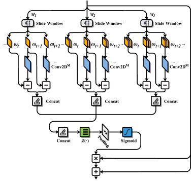
Figure 5. The structure of Hybrid Motion Enhancement Module (HMEM), where $\mathcal{O}=\left\{1,2,3\right\}$ and “Concat” denotes for concatenate operation.

3.6. Prototype Construction

Triple prior guidance are added into the raw support and query before feature extraction:

(15) $$\tilde{S}^{ck} =\left(S_{1}^{ck}+S_{2}^{ck}+S_{3}^{ck}\right)+S^{ck}=\left[\tilde{s}_{1}^{ck},\dots,\tilde{s}_{F}^{ck}\right]\in\mathbb{R}^{F\times C\times H\times W},$$

$$\tilde{Q} =\left(Q_{1}+Q_{2}+Q_{3}\right)+Q=\left[\tilde{q}_{1},\dots,\tilde{q}_{F}\right]\in\mathbb{R}^{F\times C\times H\times W}.$$

$\tilde{S}^{ck}$ and $\tilde{Q}$ are sent to the backbone network. Features of support and query are defined as:

(16) $$S_{f}^{ck} =\left[f_{\theta}\left(\tilde{s}_{1}^{ck}\right)+f_{pe}\left(1\right),\dots,f_{\theta}\left(\tilde{s}_{F}^{ck}\right)+f_{pe}\left(F\right)\right]\in\mathbb{R}^{F\times D},$$

$$Q_{f} =\left[f_{\theta}\left(\tilde{q}_{1}\right)+f_{pe}\left(1\right),\dots,f_{\theta}\left(\tilde{q}_{F}\right)+f_{pe}\left(F\right)\right]\in\mathbb{R}^{F\times D}.$$

$f_{\theta}\left(\cdot\right):\mathbb{R}^{C\times H\times W}\mapsto\mathbb{R}^{D}$ is the backbone for embedding each frame into a $D$-dimensional vector. While $f_{pe}\left(\cdot\right)$ represents the position embedding function, which can be a cosine/sine function or a learnable function, it is important to note that the function type can impact the performance of the model.
Three linear layers including $\Psi\left(\cdot\right),\Gamma\left(\cdot\right):\mathbb{R}^{F\times D}\mapsto\mathbb{R}^{F\times{d_{k}}}$ and $\Lambda\left(\cdot\right):\mathbb{R}^{F\times D}\mapsto\mathbb{R}^{F\times{d_{v}}}$ are applied for constructing the prototype of support $P^{c}$, refers to:

(17) $$A^{ck} =\mathrm{LN}\left(\Psi\left(Q_{f}\right)\right)\cdot\mathrm{LN}\left(\Gamma\left(S_{f}^{ck}\right)\right),$$

$$P^{c} =\frac{1}{K}\sum_{k=1}^{K}{\left(\mathrm{Softmax}\left(A^{ck}\right)\cdot\Lambda\left(S_{f}^{ck}\right)\right)}.$$

The $\mathrm{LN}\left(\cdot\right)$ means the layer normalization and $\mathrm{Softmax}\left(\cdot\right)$ represents the Softmax function.

3.7. Training Objective

The linear layer $\Lambda\left(\cdot\right)$ is applied on $Q_{f}$ to ensure the same operation as $S_{f}^{ck}$. By obtaining the closest distance between $Q_{f}$ and $P^{c}$, model can predict the label $\tilde{y}$ of $Q$, as:

(18) $$\tilde{y}=\underset{c}{\mathrm{arg}\min}\,\,\underset{D\left(Q,S^{c}\right)}{\underbrace{\left\|P^{c}-\left(\Lambda\left(Q_{f}\right)\right)\right\|}}.$$

The cross-entropy loss $\mathcal{L}_{\mathrm{ce}}$ is selected as the objective loss for training, which can be calculated with the ground truth $y$:

(19) $$\mathcal{L}_{\mathrm{ce}}=-\frac{1}{N}\sum_{i=1}^{N}{y_{i}\log\left(\tilde{y}_{i}\right)}.$$

Table 1. Performance ($\uparrow$ Acc. %) comparison. “$\star$”: our implementation, “$\dagger$”: multimodal methods, “N/A”: not available in the publication, Bold texts: the best results, underline texts: the previous best results.

Methods	Backbone	SthSthV2		Kinetics		UCF101		HMDB51
		1-shot	5-shot	1-shot	5-shot	1-shot	5-shot	1-shot	5-shot
CMN (Zhu and Yang, 2018, 2020)	ResNet-50	36.2	42.8	60.5	78.9	N/A	N/A	N/A	N/A
OTAM (Cao et al., 2020)	ResNet-50	42.8	52.3	73.0	85.8	N/A	N/A	N/A	N/A
ITANet (Zhang et al., 2021)	ResNet-50	49.2	62.6	73.6	84.3	N/A	N/A	N/A	N/A
TA2N (Li et al., 2022)	ResNet-50	47.6	61.0	72.8	85.8	81.9	95.1	59.7	73.9
LSTC (Luo et al., 2022)	ResNet-50	47.6	66.7	73.4	86.5	85.7	96.5	60.9	76.8
STRM (Thatipelli et al., 2022)	ResNet-50	N/A	68.1	N/A	86.7	N/A	96.9	N/A	76.3
HCL (Zheng et al., 2022)	ResNet-50	47.3	64.9	73.7	85.8	82.6	94.5	59.1	76.3
SloshNet (Xing et al., 2023a)	ResNet-50	46.5	68.3	N/A	87.0	N/A	97.1	N/A	77.5
SA-CT (Zhang et al., 2023)	ResNet-50	48.9	69.1	71.9	87.1	85.4	96.4	60.4	78.3
GCSM (Yu et al., 2023)	ResNet-50	N/A	N/A	74.2	88.2	86.5	97.1	61.3	79.3
GgHM (Xing et al., 2023b)	ResNet-50	54.5	69.2	74.9	87.4	85.2	96.3	61.2	76.9
⋆TRX (Perrett et al., 2021)	ResNet-50	55.8	69.8	74.9	85.9	85.7	96.3	66.5	77.2
⋆HyRSM (Wang et al., 2022)	ResNet-50	54.1	68.7	73.5	86.2	83.6	94.6	60.1	76.2
⋆MoLo (Wang et al., 2023b)	ResNet-50	56.6	70.7	75.2	85.7	86.2	95.4	67.1	77.3
†AmeFu-Net (Fu et al., 2020)	ResNet-50	N/A	N/A	74.1	86.8	85.1	95.5	60.2	75.5
†MTFAN (Wu et al., 2022)	ResNet-50	45.7	60.4	74.6	87.4	84.8	95.1	59.0	74.6
†AMFAR (Wanyan et al., 2023)	ResNet-50	61.7	79.5	80.1	92.6	91.2	99.0	73.9	87.8
⋆†Lite-MKD (Liu et al., 2023)	ResNet-50	55.7	69.9	75.0	87.5	85.3	96.8	66.9	74.7
SOAP-Net (Ours)	ResNet-50	61.9	79.8	81.1	93.8	94.1	99.3	76.5	88.4
STRM (Thatipelli et al., 2022)	ViT-B	N/A	70.2	N/A	91.2	N/A	98.1	N/A	81.3
SA-CT (Zhang et al., 2023)	ViT-B	N/A	66.3	N/A	91.2	N/A	98.0	N/A	81.6
⋆TRX (Perrett et al., 2021)	ViT-B	57.2	71.4	76.3	87.5	88.9	97.2	66.9	78.8
⋆HyRSM (Wang et al., 2022)	ViT-B	58.8	71.3	76.8	92.3	86.6	96.4	69.6	82.2
⋆MoLo (Wang et al., 2023b)	ViT-B	61.1	71.7	78.9	95.8	88.4	97.6	71.3	84.4
†CLIP-FSAR (Wang et al., 2023a)	ViT-B	61.9	72.1	89.7	95.0	96.6	99.0	75.8	87.7
SOAP-Net (Ours)	ViT-B	66.7	81.2	89.9	95.5	96.8	99.5	79.3	89.8

4. Experiments

4.1. Experimental Configuration

4.1.1. Datasets Processing.

We select four widely used datasets, i.e., SthSthV2 (Goyal et al., 2017), Kinetics (Carreira and Zisserman, 2017), UCF101 (Soomro et al., 2012), and HMDB51 (Kuehne et al., 2011). Apart from SthSthV2, which is temporal-related, other three datasets are all spatial-related. When decoding videos, we set the sampling intervals to every 1 frame. For simulating various fluency, the intervals can be adjusted. Building upon data split from prior works (Zhu and Yang, 2018; Cao et al., 2020; Zhang et al., 2020), we split our datasets into training, validation, and testing sets. A task within each set, classifying query samples into one of the support classes serves as a training unit.
Following TSN (Wang et al., 2016), 8 frames ($F=8$) resized to $3\times 256\times 256$ are uniformly and sparsely sampled each time. Data augmentations in training include random crops to $3\times 224\times 224$ and horizontal flipping, while only a center crop is used during testing. As pointed out in previous works (Cao et al., 2020), many action classes in SthSthV2 are sensitive to horizontal direction (e.g., “Pulling S from left to right”). Hence, we avoid horizontal flipping on this dataset.

4.1.2. Implementation Details and Evaluation.

In 3DEM, the size of $\mathrm{Conv3D}$ is $3\times 3\times 3$. For CWEM, the expand channel number $C_{r}$ is set to 16, while $\mathrm{Conv1D}$ size is $3$. We set $\mathcal{O}=\left\{1,2,3\right\}$ in HMEM, the $\mathrm{Conv2D}^{M}$ with shared parameters are also $3\times 3$ in each branch. All 2D convolution for changing channel number is set to $1\times 1$. Except for these channel recovery convolutions, other convolutions maintain the same shape of input and output. We employ widely-used ResNet-50 (He et al., 2016) or ViT-B (Dosovitskiy et al., 2020) as the backbone initialized with pre-trained weights on ImageNet (Deng et al., 2009). The final outputs of the backbone are 2048-dimensional vectors ($D=2048$). For three linear layers, the parameters are randomly initialized while $d_{k}$ and $d_{v}$ are both set to 1152.
We utilize the standard 5-way 5-shot and 1-shot few-shot settings. Due to its larger size, SthSthV2 requires 75,000 tasks for training, while other datasets employ 10,000 tasks. An SGD optimizer is applied to train our model, with an initial learning rate of $10^{-3}$. The training process is conducted on a deep learning server equipped with two NVIDIA 24GB RTX3090 GPUs. Validation set determines hyperparameters. During testing, we report average accuracy across 10,000 random tasks from the testing set.

4.2. Comparison with Various Methods

4.2.1. Comparison with ResNet-50 Backbone Methods.

Based on the average accuracy reported in Table 1, we have the following observation. Our SOAP-Net outperforms other methods and achieves SOTA performance. For example, on the Kinetics dataset under the 1-shot setting, SOAP improves the current SOTA performance of MoLo (Wang et al., 2023b) from 75.2% to 81.1%. We believe the motion information within adjacent frames is insufficient, despite MoLo introducing it. Similar improvements are also found in other datasets under diverse few-shot settings, showing that spatio-temporal relation and comprehensive motion information from SOAP lead to significant improvement in FSAR. It is worth mentioning that SOAP-Net even surpasses multimodal methods.

4.2.2. Comparison with ViT-B Backbone Methods.

ResNet-50 serves as the backbone network in most previous works, while ViT-B is rarely used in FSAR. For a comprehensive comparison, we implemented several methods and replaced their backbones with ViT-B, finding it outperformed ResNet-50 in FSAR due to larger model capacity. The previous SOTA performance is also achieved by MoLo, benefiting from optimizing spatio-temporal relation construction and comprehensive motion information. A similar trend is observed on ResNet-50 and ViT-B. These comparisons reveal the competitiveness of our proposed method.

4.3. Essential Components and Factors

4.3.1. Analysis of Key Components.

We first divide SOAP into three key components: 3DEM, CWEM, and HMEM. Experiments on individual or combined components are conducted on two datasets under diverse few-shot settings. As shown in Table 2, results indicate that each SOAP component can improve FSAR performance. However, the most significant boost comes from HMEM, likely due to fuller motion information usage. Combining two components with HMEM performs better than without HMEM. We conclude that comprehensive motion information plays a more significant role in FSAR. Using all SOAP components yields the best results, proving all are essential.

Table 2. Analysis ($\uparrow$ Acc. %) of Key Components.

3DEM	CWEM	HMEM	SthSthV2		Kinetics
			1-shot	5-shot	1-shot	5-shot
✘	✘	✘	54.5	67.3	74.1	85.2
✔	✘	✘	55.6	69.4	76.8	86.6
✘	✔	✘	55.4	70.2	76.1	86.1
✘	✘	✔	58.3	72.3	78.5	88.9
✔	✔	✘	58.5	73.1	78.8	89.3
✘	✔	✔	60.5	77.8	79.0	92.2
✔	✘	✔	60.7	78.5	80.2	92.6
✔	✔	✔	61.9	79.8	81.1	93.8

4.3.2. Frame Tuples and Branches Design.

Results under various hyperparameter $\mathcal{O}$ settings of HMEM is demonstrated in Table 3. Each element represents frame counts, with the cardinality of set $\left|\mathcal{O}\right|$ equaling number of branches. Performance generally improves with more branches. Specifically, any frame tuple size improves with HMEM having one branch. Better results occur with two branches. Best performance occurs at 3 branches under $\mathcal{O}=\left\{1,2,3\right\}$ setting. This aligns with intuition comprehensive motion information contributes more for FSAR. However, excessive branches risk degradation. Too much motion information overlap does not provide useful information. For example, $\mathcal{O}=\left\{4\right\}$ acts similarly to two $\mathcal{O}=\left\{2\right\}$ configurations together, implying that they perform worse than other non-overlapping settings. While $\mathcal{O}=\left\{1\right\}$ provides motion information between frames not conflicting with other $\mathcal{O}$ settings for building frame tuples, introducing comprehensive motion information.

Table 3. Impact ($\uparrow$ Acc. %) of $\mathcal{O}$ Design.

$\mathcal{O}$ Design	SthSthV2		Kinetics
	1-shot	5-shot	1-shot	5-shot
$\mathcal{O}=\left\{1\right\}$	59.1	73.9	78.9	89.5
$\mathcal{O}=\left\{2\right\}$	59.5	74.3	79.1	90.8
$\mathcal{O}=\left\{3\right\}$	59.4	74.6	79.5	90.8
$\mathcal{O}=\left\{4\right\}$	59.5	74.2	79.3	90.5
$\mathcal{O}=\left\{1,2\right\}$	60.6	77.6	80.3	92.3
$\mathcal{O}=\left\{1,3\right\}$	60.7	77.8	80.1	92.4
$\mathcal{O}=\left\{1,4\right\}$	60.4	78.2	80.5	92.4
$\mathcal{O}=\left\{2,3\right\}$	60.7	78.3	80.5	92.1
$\mathcal{O}=\left\{2,4\right\}$	60.1	77.2	80.0	91.9
$\mathcal{O}=\left\{3,4\right\}$	60.4	78.3	80.2	92.9
$\mathcal{O}=\left\{1,2,3\right\}$	61.9	79.8	81.1	93.8
$\mathcal{O}=\left\{1,2,4\right\}$	60.7	77.9	80.5	92.6
$\mathcal{O}=\left\{1,3,4\right\}$	61.9	79.3	80.7	93.5
$\mathcal{O}=\left\{2,3,4\right\}$	60.7	77.7	80.3	92.3
$\mathcal{O}=\left\{1,2,3,4\right\}$	61.5	79.2	80.7	92.8

4.3.3. The Impact of Temporal Order.

Up to this point, we believe the frame tuple should follow the temporal order for better representation. After determining $\mathcal{O}=\left\{1,2,3\right\}$ setting, we conduct experiments with temporal and reversed order. In an extreme scenario, the frames in support take the temporal order while frames in query are reversely ordered during inference. As the results in Table 4, SthSthV2 and Kinetics datasets both have a drop with reversed order settings. However, the drop in SthSthV2 is much larger than in Kinetics. The dataset type supports our previous observation that the temporal-related SthSthV2 is more sensitive to order than the spatial-related Kinetics. Based on above results, we can infer that SOAP is closely tied to temporal order.

Table 4. Impact ($\uparrow$ Acc. %) of Temporal Order.

Reversed Order	SthSthV2		Kinetics
	1-shot	5-shot	1-shot	5-shot
✔	54.1	66.6	79.2	91.6
✘	61.9	79.8	81.1	93.8

4.4. Research on How SOAP Works

4.4.1. CAM Visualization.

The CAM (Selvaraju et al., 2017) for “crossing river” from the Kinetics dataset is shown in Figure 6. The first row shows raw HFR video frames. We observe that the timeline and displacement of the moving peoples are very subtle, making it difficult to detect the spatio-temporal relation and motion information. In the second row, we see that the model attends more to the background than moving peoples. This result supports our observation in HFR videos. With the help of SOAP, we detect that the focus shifts from the background to the moving peoples, despite the subtle timeline and displacement. Based on this analysis of the CAM, we conclude that motion information is crucial in FSAR. Spatio-temporal relation and comprehensive motion information from SOAP can significantly improve feature representation.

\begin{overpic}[width=195.12767pt]{figures/CAM3.pdf} \put(47.0,50.0){\footnotesize Raw} \put(44.0,32.0){\footnotesize w/o SOAP} \put(44.0,14.0){\footnotesize w/ SOAP} \end{overpic}

Figure 6. Example of the “crossing river” selected from Kinetics, timeline is from left to right.

4.4.2. T-SNE Visualization.

In the 5-way task, feature distributions can be visualized using t-SNE (Van der Maaten and Hinton, 2008). We select five representative yet challenging support action classes from Kinetics: “ski jumping”, “snowboarding”, “skateboarding”, “crossing river”, and “driving tractor”. The t-SNE visualization is shown in Figure 7, with different colors and markers representing distinct action classes. Without SOAP (Figure 7(a)), the five classes are generally separable but with some overlapping, such as in the right (“driving tractor” and “crossing river”), left (“skateboarding” and “snowboarding”), and center (“ski jumping”). By contrast, with SOAP (Figure 7(b)), the five classes are more distinctly separated and same-class samples are more tightly clustered. This strong evidence demonstrates the enhanced representational ability of SOAP for support features.

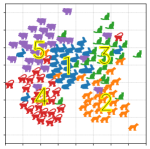
(a) w/o SOAP

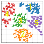
(b) w/ SOAP

Figure 7. T-SNE visualization of five action classes in support from Kinetics. Blue Rabbits: “ski jumping”, Orange Dogs: “crossing river”, Green Cats: “driving tractor”, Red Monkeys: “snowboarding”, Purple Pigs: “skateboarding”.

4.5. Pluggability of SOAP

4.5.1. On RGB-Based Methods.

In Table 5, we experimentally demonstrate that the SOAP generalizes well to other methods by inserting it into widely used methods including TRX, HyRSM, and MoLo. Using Kinetics as an example, TRX benefits from comprehensive motion information and achieves 7.6% gains in the 1-shot setting and 8.5% in the 5-shot setting. Similar improvements are also observed in the other two methods. These results fully prove that optimizing spatio-temporal relation and comprehensive motion information are particularly useful for feature extraction.

Table 5. Pluggability ($\uparrow$ Acc. %) on RGB-Based Methods.

RGB-Based Methods	SthSthV2		Kinetics
	1-shot	5-shot	1-shot	5-shot
TRX	55.8	69.8	74.9	85.9
SOAP-TRX	62.3	80.3	82.5	94.4
HyRSM	54.1	68.7	73.5	86.2
SOAP-HyRSM	60.1	75.8	79.9	91.6
MoLo	56.6	70.7	75.2	85.7
SOAP-MoLo	60.9	76.6	79.6	92.1

4.5.2. On Multimodal Methods.

Backbone networks serve as feature extractors in multimodal methods for FSAR. Additional information from other modalities enhances performance. In most multimodal methods, depth or optical flow information augments RGB data. Apart from the RGB backbone, additional depth-specific or optical-flow-specific networks are also utilized. As depth and optical flow are both derived from raw RGB frames, they inherently contain spatio-temporal relation and motion information. Therefore, we hypothesize SOAP can also benefit multimodal methods and implement several multimodal methods equipped with SOAP for evaluation. Results in Table 6 demonstrate that all selected multimodal methods achieve further improvement via optimized spatio-temporal relation construction and comprehensive motion information capturing from SOAP. These results provide legitimate validation for our hypothesis and emphasize the advanced pluggability of SOAP on multimodal methods.

Table 6. Pluggability ($\uparrow$ Acc. %) on Multimodal Methods.

Multimodal Methods	SthSthV2		Kinetics
	1-shot	5-shot	1-shot	5-shot
AmeFu-Net	56.2	71.1	76.3	88.2
SOAP-AmeFu-Net	62.5	80.4	82.2	94.6
MTFAN	55.8	70.6	74.8	87.8
SOAP-MTFAN	62.2	81.3	81.6	93.7
Lite-MKD	55.7	69.9	75.0	87.5
SOAP-Lite-MKD	61.8	80.6	81.1	93.2
AMFAR	61.3	78.9	79.3	91.4
SOAP-AMFAR	64.7	82.6	83.9	95.3

4.6. Generalization Study

In this study, we aim to simulate different levels of frame-rate by varying the sampling interval from a minimum of 1 to a maximum of 6 and conduct a series of experiments under a well-established 5-way 5-shot setting. As shown in Figure 8, the performance tends to decrease gradually with the increase of frame-rate. We find that recent FSAR methods all experience drastic degradation in performance with HFR videos while SOAP-Net indicates performance stability, demonstrating the superiority of SOAP across varying frame-rate. These phenomena also highlight the key role of spatio-temporal relation optimization and comprehensive motion information in advancing FSAR performance.

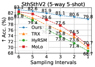
(a) SthSthV2

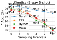
(b) Kinetics

Figure 8. Performance ($\uparrow$ Acc. %) of Various Frame-Rates.

5. Conclusion

In this paper, we propose the plug-and-play SOAP to optimize spatio-temporal relation construction and capture comprehensive motion information for FSAR. SOAP takes into account temporal connections across feature channels and spatio-temporal relation within features. It combines frame tuples of various frame counts to provide a broader perspective for motion information. Considering the competitiveness, pluggability, generalization, and robustness of SOAP, we hope and believe that our work will offer valuable insights for future research in multimedia analytic.

Supplementary Material

In the Supplementary Material, we provide:

• Partial Generalization Study.

• Robustness Study.

• Additional CAM Visualizations.

• Configuration of hyperparameters.

• Pseudo-code for a better understanding.

Appendix A Generalization Study

A.1. Generalization on More Complex Tasks

In a range of real-world scenarios, tasks are often more complex than a mere 5-way classification. Recognizing this complexity, we seek to enhance the challenge of these tasks by augmenting the number of ways (classes). Experiments are conducted on SthSthV2 and Kinetics. From Figure I, performance of various methods (Perrett et al., 2021; Wang et al., 2022, 2023b) decreases with increasing complexity. Although task complexity hinders performance boosts, SOAP-Net consistently outperforms other methods. Surprisingly, SOAP-Net decays less than other methods on complex tasks. The above results show better generalization of SOAP on more complex tasks. It also indicates spatio-temporal relation and comprehensive motion information support better generalization.

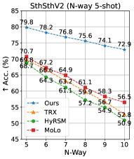
(a) SthSthV2

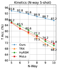
(b) Kinetics

Figure I. Performance ($\uparrow$ Acc. %) of More Complex Tasks.

A.2. Generalization on Any-Shot Setting

In real-word applications, it is often challenging to ensure that every task has an equal number of samples. To create a more authentic testing environment for assessing the generalization ability of SOAP, we utilize a shot number in the range of 1 to 5, effectively establishing an any-shot setting for our experiments. Results with 95% confidence intervals are shown in Table I. SOAP-Net outperforms three recent methods under the any-shot setting, and shows similar performance in normal 1-shot or 5-shot settings. The confidence intervals indicate that our SOAP-Net exhibits more stable performance under the more realistic evaluation scenario. The above experiments underscore the potential of SOAP in practical applications.

Table I. Any-shot Performance ($\uparrow$ Acc. %) comparison.

Methods	SthSthV2	Kinetics
TRX	61.3 ($\pm$0.5)	79.3 ($\pm$0.4)
HyRSM	62.2 ($\pm$0.6)	79.5 ($\pm$0.5)
MoLo	63.7 ($\pm$0.4)	80.9 ($\pm$0.3)
SOAP-Net	70.2 ($\pm$0.3)	87.4 ($\pm$0.2)

Appendix B Robustness Study

B.1. Robustness on Sample-Level Noise

In a more authentic testing environment, noise inevitably occurs during sample collection, and removing it incurs additional costs. Specifically, a particular class might be mixed with samples from other classes. As shown in Figure II, directly replacing one or more samples with noise within a few-shot task during inference is called sample-level noise. Evaluating FSAR methods with sample-level noise simulates more realistic sample scenarios. For a clear demonstration, we conduct 10-shot experiments and reveal the results in Table II. In general, performance decreases with increasing noise. For every 10% increase in the sample-level noise ratio, performance drops by about 4%. Although the overall trend remains regardless of the method, we observe a distinction between SOAP-Net and other methods. The performance decrease with the sample-level noise ratio for SOAP-Net is about 2%, much less than others. The stable performance against sample-level noise highlights superior robustness of our SOAP.

\begin{overpic}[width=182.1196pt]{figures/sample_noise.pdf} \put(15.0,72.0){\footnotesize 1} \put(26.0,72.0){\footnotesize 2} \put(37.0,72.0){\footnotesize 3} \put(48.0,72.0){\footnotesize 4} \put(59.0,72.0){\footnotesize 5} \put(70.0,72.0){\footnotesize 6} \put(81.0,72.0){\footnotesize 7} \put(92.0,72.0){\footnotesize 8} \put(-5.0,65.0){\footnotesize Sample 1} \put(-5.0,50.0){\footnotesize Sample 2} \put(-5.0,35.0){\footnotesize Sample 3} \put(-5.0,20.0){\footnotesize Sample 4} \put(-5.0,5.0){\footnotesize{{\color[rgb]{1,0,0}Sample 5}}} \end{overpic}

Figure II. The 5-shot example of “snowboarding”, where the sample-level noise is highlighted by red box. Sample-level noise means directly replacing a pure sample with noise within a few-shot task.

Table II. Evaluation ($\uparrow$ Acc. %) with Sample-Level Noise.

Datasets	Methods	Sample-Level Noise Ratio
		0%	10%	20%	30%	40%
SthSthV2	TRX	74.4	69.9	66.3	62.6	57.2
	HyRSM	73.6	68.9	64.3	60.9	54.9
	MoLo	75.3	71.6	67.1	64.0	59.8
	SOAP-Net	84.9	83.2	81.6	79.1	77.9
Kinetics	TRX	90.1	86.9	82.4	77.8	73.2
	HyRSM	89.7	85.6	81.4	77.2	72.9
	MoLo	90.6	86.2	82.3	76.8	70.1
	SOAP-Net	96.4	94.1	91.9	89.6	87.7

B.2. Robustness on Frame-Level Noise

Due to the uncertainty of video recorder, it is not guaranteed that the view of all frames is aligned with the moving subject. In some undesirable cases, multiple irrelevant frames are mixed in. Under such conditions, higher requirements are placed on the FSAR method. As shown in Figure III, we replace some pure frames with irrelevant frames from other action classes during inference. We define this as frame-level noise. The 5-way 10-shot setting is the same as the evaluation, and the results are detailed in Table III. Compared to sample-level noise, the negative impact of frame-level noise is small, with a similar overall trend. SOAP-Net outperforms other methods under any frame-level noise number. We find the impact of frame noise on TRX and HyRSM is greater than on MoLo and our SOAP-Net. The commonality of MoLo and SOAP-Net is both apply motion information, which plays a vital role in FSAR. Our proposed method is less affected, proving comprehensive motion information provides better robustness to frame-level noise.

\begin{overpic}[width=182.1196pt]{figures/frame_noise.pdf} \put(15.0,72.0){\footnotesize{{\color[rgb]{1,0,0}1}}} \put(26.0,72.0){\footnotesize{{\color[rgb]{1,0,0}2}}} \put(37.0,72.0){\footnotesize{{\color[rgb]{1,0,0}3}}} \put(48.0,72.0){\footnotesize 4} \put(59.0,72.0){\footnotesize 5} \put(70.0,72.0){\footnotesize{{\color[rgb]{1,0,0}6}}} \put(81.0,72.0){\footnotesize{{\color[rgb]{1,0,0}7}}} \put(92.0,72.0){\footnotesize 8} \put(-5.0,65.0){\footnotesize Sample 1} \put(-5.0,50.0){\footnotesize Sample 2} \put(-5.0,35.0){\footnotesize Sample 3} \put(-5.0,20.0){\footnotesize Sample 4} \put(-5.0,5.0){\footnotesize Sample 5} \end{overpic}

Figure III. The 5-shot example of “snowboarding”, where the frame-level noise is highlighted by red box. Frame-level noise means introducing noise frames.

Table III. Evaluation ($\uparrow$ Acc. %) with Frame-Level Noise.

Datasets	Methods	Frame-Level Noise Number
		0	1	2	3	4
SthSthV2	TRX	74.4	71.5	68.4	65.1	62.2
	HyRSM	73.6	70.2	66.9	64.2	61.1
	MoLo	75.3	74.1	72.2	70.1	68.8
	SOAP-Net	84.9	84.2	83.6	82.2	80.9
Kinetics	TRX	90.1	87.3	84.8	81.2	79.0
	HyRSM	89.7	86.5	84.4	82.2	80.1
	MoLo	90.6	89.5	88.3	87.0	85.8
	SOAP-Net	96.4	95.5	94.3	93.1	91.7

Appendix C Additional CAM Visualizations

As a complement to the CAM visualization in the main paper, we provide additional examples in Figure IV. For the example “snowboarding”, each frame is sampled without much background variation. However, the high fluency makes motion information weak, and the model attention mistakenly focuses on the background. Fortunately, the model with SOAP concentrates more on the skier instead of the outlying background. Due to disordered scenery like driftwood and tourists, the example “diving cliff” is more complex than the first. In the second row, we can clearly see the model is disrupted and does not know where to focus. When motion information is highlighted, people diving the cliff is easier to find.

\begin{overpic}[width=195.12767pt]{figures/CAM2.pdf} \put(47.0,50.0){\footnotesize Raw} \put(44.0,32.0){\footnotesize w/o SOAP} \put(44.0,14.0){\footnotesize w/ SOAP} \end{overpic}

(a) Example “snowboarding”.

\begin{overpic}[width=195.12767pt]{figures/CAM1.pdf} \put(47.0,50.0){\footnotesize Raw} \put(44.0,32.0){\footnotesize w/o SOAP} \put(44.0,14.0){\footnotesize w/ SOAP} \end{overpic}

(b) Example “diving cliff”.

Figure IV. Additional CAM Visualizations.

Appendix D Hyperparameter Study

Table IV illustrates the SOAP-Net structure in our implementation, as detailed in the main paper. The $\mathrm{Conv3D}$ size is $3\times 3\times 3$ in 3DEM. In CWEM, the expand channel number $C_{r}$ is set to 16, while $\mathrm{Conv1D}$ size is $3$. $\mathcal{O}=\left\{1,2,3\right\}$ and the $\mathrm{Conv2D}^{M}$ sizes are $3\times 3$ in HMEM. For a supplementary interpretation of implementation details, extensive experiments are conducted on individual modules with diverse configuration to determine the optimal hyperparameters.

Table IV. Structure of SOAP-Net. Notations are consistent with the main paper.

Modules / Operation	Input	Input Size	Output	Onput Size
3DEM	$S^{ck}$	[8,3,224,224]	$\hat{S}_{1}^{ck}$	[8,1,224,224]
	$Q$	[8,3,224,224]	$\hat{Q}_{1}$	[8,1,224,224]
CWEM	$S^{ck}$	[8,3,224,224]	$\dot{S}_{2}^{ck}$	[8,3,1,1]
	$Q$	[8,3,224,224]	$\dot{Q}_{2}$	[8,3,1,1]
HMEM	$S^{ck}$	[8,3,224,224]	$\hat{S}_{3}^{ck}$	[8,3,1,1]
	$Q$	[8,3,224,224]	$\hat{Q}_{3}$	[8,3,1,1]
Eqn.(15)	$S^{ck}$	[8,3,224,224]	$\tilde{S}^{ck}$	[8,3,224,224]
	$S_{1}^{ck}$	[8,3,224,224]
	$S_{2}^{ck}$	[8,3,224,224]
	$S_{3}^{ck}$	[8,3,224,224]
	$Q$	[8,3,224,224]	$\tilde{Q}$	[8,3,224,224]
	$Q_{1}$	[8,3,224,224]
	$Q_{2}$	[8,3,224,224]
	$Q_{3}$	[8,3,224,224]
Eqn.(16)	$\tilde{S}^{ck}$	[8,3,224,224]	$S_{f}^{ck}$	[8,2048]
	$\tilde{Q}$	[8,3,224,224]	$Q_{f}$	[8,2048]

D.1. Hyperparameter Study of 3DEM

The size of the $\mathrm{Conv3D}$ plays a crucial role as the main hyperparameter in 3DEM. As a result, we only apply 3DEM to conduct few-shot experiments on two datasets and have reported the results in Table V. In most cases, the best performance appears in the $3\times 3\times 3$ row. Based on these findings, we conclude that the $3\times 3\times 3$ $\mathrm{Conv3D}$ is the optimal hyperparameter for 3DEM.

Table V. Hyperparameter Study ($\uparrow$ Acc. %) of 3DEM.

$\mathrm{Conv3D}$	SthSthV2		Kinetics
	1-shot	5-shot	1-shot	5-shot
$1\times 1\times 1$	54.9	67.6	74.6	85.7
$3\times 3\times 3$	55.6	69.4	76.8	86.6
$5\times 5\times 5$	55.1	69.5	76.6	86.3
$7\times 7\times 7$	54.6	68.2	75.9	85.8

D.2. Hyperparameter Study of CWEM

The size of $\mathrm{Conv1D}$ and the expand channel number $C_{r}$ are essential primary hyperparameters. A well-matched combination can effectively calibrate temporal connections between each channel. Therefore, after arranging and combining these two hyperparameters, we present all results using only CWEM in Table VI. Our findings indicate that $\mathrm{Conv1D}$ with sizes of 3 or 5 outperforms those with sizes of 1 or 7. Further experiments on $C_{r}$ reveal that $C_{r}=16$ contributes to optimal performance in most cases. Taking a comprehensive consideration based on reported results, we conclude that $\mathrm{Conv1D}$ with a size of 3 and $C_{r}=16$ represents the best set of hyperparameters for CWEM.

Table VI. Hyperparameter Study ($\uparrow$ Acc. %) of CWEM.

		SthSthV2		Kinetics
$\mathrm{Conv1D}$	$C_{r}$	1-shot	5-shot	1-shot	5-shot
	8	54.5	67.3	74.2	85.3
	16	54.7	67.6	74.4	85.6
	32	54.6	67.4	74.4	85.4
1	64	54.5	67.4	74.3	85.6
	8	55.1	69.6	75.7	85.8
	16	55.4	70.2	76.1	86.1
	32	55.4	70.0	75.8	85.9
3	64	55.2	69.7	75.7	85.5
	8	54.8	69.1	75.2	85.5
	16	55.1	69.3	75.7	85.8
	32	55.2	69.3	75.5	85.6
5	64	55.1	69.2	75.3	85.9
	8	54.2	67.4	74.1	85.1
	16	54.6	67.6	74.2	85.5
	32	54.5	67.5	74.3	85.6
7	64	54.3	67.3	74.2	85.2

D.3. Hyperparameter Study of HMEM

Similar to CWEM, HMEM also has two hyperparameters: the size of $\mathrm{Conv2D}^{M}$ and the design of $\mathcal{O}$. The former determines the visual receptive field size, while the latter determines the number of branches and frame tuple sizes. The results obtained using only HMEM through permutation and combination are presented in Table VII. Performance with $3\times 3$ and $5\times 5$ $\mathrm{Conv2D}^{M}$ is slightly better than other settings. As indicated in the main paper, performance generally improves with more branches, but excessive branches can lead to degradation. Considering the $\mathcal{O}$ design, it is confirmed that a configuration of $3\times 3$ $\mathrm{Conv2D}^{M}$ with $\mathcal{O}=\left\{1,2,3\right\}$ is the most suitable hyperparameter setting for HMEM.

Table VII. Hyperparameter Study ($\uparrow$ Acc. %) of HMEM.

$\mathrm{Conv2D}^{M}$	$\mathcal{O}$ Design	SthSthV2		Kinetics
		1-shot	5-shot	1-shot	5-shot
$1\times 1$	$\mathcal{O}=\left\{3\right\}$	57.1	71.8	77.2	87.3
	$\mathcal{O}=\left\{2,3\right\}$	57.5	72.1	77.6	87.8
	$\mathcal{O}=\left\{1,2,3\right\}$	57.9	72.1	78.1	88.6
	$\mathcal{O}=\left\{1,2,3,4\right\}$	57.3	71.4	77.1	87.2
$3\times 3$	$\mathcal{O}=\left\{3\right\}$	57.6	71.4	77.7	88.1
	$\mathcal{O}=\left\{2,3\right\}$	57.8	71.9	78.2	88.7
	$\mathcal{O}=\left\{1,2,3\right\}$	58.3	72.3	78.5	88.9
	$\mathcal{O}=\left\{1,2,3,4\right\}$	57.2	71.0	77.6	88.0
$5\times 5$	$\mathcal{O}=\left\{3\right\}$	57.5	71.9	77.5	88.2
	$\mathcal{O}=\left\{2,3\right\}$	57.8	72.2	77.7	88.4
	$\mathcal{O}=\left\{1,2,3\right\}$	58.1	72.1	78.2	88.7
	$\mathcal{O}=\left\{1,2,3,4\right\}$	57.1	71.6	77.2	87.7
$7\times 7$	$\mathcal{O}=\left\{3\right\}$	57.6	70.4	76.2	87.3
	$\mathcal{O}=\left\{2,3\right\}$	58.0	70.8	76.6	87.5
	$\mathcal{O}=\left\{1,2,3\right\}$	57.9	71.1	77.3	88.1
	$\mathcal{O}=\left\{1,2,3,4\right\}$	56.8	70.2	76.1	87.1

Appendix E Pseudo-code

For a better understanding of HMEM, we provide a summary of the two main processes: the sliding window algorithm (Algorithm 1) and motion information calculation (Algorithm 2), using pseudocode. Both processes consist of one layer loops with a computational complexity of $O\left(N_{\mathrm{w}}\right)$ due to $\left|\mathcal{S}_{t}\right|=N_{\mathrm{w}}$. In order to comprehensively calculate motion information (Algorithm 3), the above two algorithms are included in a larger loop for hyperparameter $\mathcal{O}$ set. As a result, the computational complexity of the entire HMEM is $O\left(\left|\mathcal{O}\right|N_{\mathrm{w}}\right)$.

Input: $I=\left[I_{1},\dots,I_{F}\right]\in\mathbb{R}^{F\times C\times H\times W}$, $T~{}\left(T\in\mathcal{O},T<F,T\in\mathbb{N}^{*}\right)$

Output: $\mathcal{S}_{t}$

1 $F\leftarrow\textnormal{{Shape}}\left(I,0\right)$ ; $N_{\mathrm{w}}\leftarrow F-T+1$;

$\mathcal{S}_{t}\leftarrow\varnothing$;

  // Defining an empty list

2 for each $i\in\left[0,N_{\mathrm{w}}-1\right]$ do

3      $\mathcal{S}_{t}\leftarrow\textnormal{{Append}}\left(\mathcal{S}_{t},I\left[:,i:i+T,\cdots\right]\right)$;

4 end for

return $\mathcal{S}_{t}$

Algorithm 1 Sliding window algorithm $\mathrm{SW}\left(\cdot,\cdot\right)$

Input: $\mathcal{S}_{t}$

Output: $\mathcal{M}$

$\mathcal{M}\leftarrow\varnothing$;

  // Defining an empty list

1 for each $i\in\left[0,\left|\mathcal{S}_{t}\right|-1\right]$ do

       $m\leftarrow\textnormal{{Conv}}(\mathcal{S}_{t}\left[i+1\right])-\mathcal{S}_{t}\left[i\right]$;

        // $\mathrm{Conv2D}^{M}$

2       if $\mathcal{M}=\varnothing$ then

3             $\mathcal{M}\leftarrow m$;

4       end if

5      else

6            $\mathcal{M}\leftarrow\textnormal{{Concat}}\left(\left[\mathcal{M},m\right],\mathrm{dim}=0\right)$;

7       end if

8      

9 end for

return $\mathcal{M}$

Algorithm 2 Motion information calculation $\mathrm{MIC}\left(\cdot\right)$

Input: $I=\left[I_{1},\dots,I_{F}\right]\in\mathbb{R}^{F\times C\times H\times W}$, $\mathcal{O}$

Output: $\mathcal{M}_{c}$

$\mathcal{M}_{c}\leftarrow\varnothing$;

  // Defining an empty list

1 for $T\in\mathcal{O}$ do

       $\mathcal{S}_{t}\leftarrow\textnormal{{SW}}\left(I,T\right)$;

        // Slide window algorithm

       $\mathcal{M}\leftarrow\textnormal{{MIC}}\left(\mathcal{S}_{t}\right)$;

        // Motion information calculation

2       if $\mathcal{M}_{c}=\varnothing$ then

3             $\mathcal{M}_{c}\leftarrow\mathcal{M}$;

4       end if

5      else

6            $\mathcal{M}_{c}\leftarrow\textnormal{{Concat}}\left(\left[\mathcal{M}_{c},\mathcal{M}\right],\mathrm{dim}=0\right)$;

7       end if

8      

9 end for

return $\mathcal{M}_{c}$

Algorithm 3 Motion information calculation

Contribution Statement

• Wenbo Huang: Proposing the idea, implementing code, conducting experiments, data collection, figure drawing, table organizing, and completing original manuscript.

• Jinghui Zhang: Providing experimental platform, supervision, writing polish, and funding acquisition.

• Xuwei Qian: Idea improvement and writing polish.

• Zhen Wu: Data verification and writing polish.

• Meng Wang: Funding acquisition

• Lei Zhang: Rebuttal assistance and funding acquisition.

- (1)
- Cao et al. (2020) Kaidi Cao, Jingwei Ji, Zhangjie Cao, Chien-Yi Chang, and Juan Carlos Niebles. 2020. Few-shot video classification via temporal alignment. In CVPR. 10618–10627.
- Carreira and Zisserman (2017) Joao Carreira and Andrew Zisserman. 2017. Quo vadis, action recognition? a new model and the kinetics dataset. In CVPR. 6299–6308.
- Chen et al. (2021) Chun-Fu Richard Chen, Rameswar Panda, Kandan Ramakrishnan, Rogerio Feris, John Cohn, Aude Oliva, and Quanfu Fan. 2021. Deep analysis of cnn-based spatio-temporal representations for action recognition. In CVPR. 6165–6175.
- Croitoru et al. (2021) Ioana Croitoru, Simion-Vlad Bogolin, Marius Leordeanu, Hailin Jin, Andrew Zisserman, Samuel Albanie, and Yang Liu. 2021. Teachtext: Crossmodal generalized distillation for text-video retrieval. In ICCV. 11583–11593.
- Deng et al. (2009) Jia Deng, Wei Dong, Richard Socher, Li-Jia Li, Kai Li, and Feifei Li. 2009. Imagenet: A large-scale hierarchical image database. In CVPR. IEEE, 248–255.
- Dosovitskiy et al. (2020) Alexey Dosovitskiy, Lucas Beyer, Alexander Kolesnikov, Dirk Weissenborn, Xiaohua Zhai, Thomas Unterthiner, Mostafa Dehghani, Matthias Minderer, Georg Heigold, Sylvain Gelly, et al. 2020. An Image is Worth 16x16 Words: Transformers for Image Recognition at Scale. In ICLR.
- Finn et al. (2017) Chelsea Finn, Pieter Abbeel, and Sergey Levine. 2017. Model-agnostic meta-learning for fast adaptation of deep networks. In ICML. 1126–1135.
- Fu et al. (2020) Yuqian Fu, Li Zhang, Junke Wang, Yanwei Fu, and Yu-Gang Jiang. 2020. Depth guided adaptive meta-fusion network for few-shot video recognition. In ACM MM. ACM, 1142–1151.
- Goyal et al. (2017) Raghav Goyal, Samira Ebrahimi Kahou, Vincent Michalski, Joanna Materzynska, Susanne Westphal, Heuna Kim, Valentin Haenel, Ingo Fruend, Peter Yianilos, Moritz Mueller-Freitag, et al. 2017. The ”something something” video database for learning and evaluating visual common sense. In ICCV. 5842–5850.
- He et al. (2016) Kaiming He, Xiangyu Zhang, Shaoqing Ren, and Jian Sun. 2016. Deep residual learning for image recognition. In CVPR. 770–778.
- Hu et al. (2018) Jie Hu, Li Shen, and Gang Sun. 2018. Squeeze-and-excitation networks. In CVPR. 7132–7141.
- Kuehne et al. (2011) Hildegard Kuehne, Hueihan Jhuang, Estíbaliz Garrote, Tomaso Poggio, and Thomas Serre. 2011. HMDB: a large video database for human motion recognition. In ICCV. IEEE, 2556–2563.
- Li et al. (2022) Shuyuan Li, Huabin Liu, Rui Qian, Yuxi Li, John See, Mengjuan Fei, Xiaoyuan Yu, and Weiyao Lin. 2022. TA2N: Two-stage action alignment network for few-shot action recognition. In AAAI, Vol. 36. 1404–1411.
- Liu et al. (2023) Baolong Liu, Tianyi Zheng, Peng Zheng, Daizong Liu, Xiaoye Qu, Junyu Gao, Jianfeng Dong, and Xun Wang. 2023. Lite-MKD: A Multi-modal Knowledge Distillation Framework for Lightweight Few-shot Action Recognition. In ACM MM. 7283–7294.
- Liu and Ma (2019) Kun Liu and Huadong Ma. 2019. Exploring background-bias for anomaly detection in surveillance videos. In ACM MM. 1490–1499.
- Luo et al. (2022) Wenyang Luo, Yufan Liu, Bing Li, Weiming Hu, Yanan Miao, and Yangxi Li. 2022. Long-Short Term Cross-Transformer in Compressed Domain for Few-Shot Video Classification.. In IJCAI. 1247–1253.
- Pan et al. (2023) Panda Pan, Yang Zhao, Yuan Chen, Wei Jia, Zhao Zhang, and Ronggang Wang. 2023. Cross-view Resolution and Frame Rate Joint Enhancement for Binocular Video. In ACM MM. 8367–8375.
- Perrett et al. (2021) Toby Perrett, Alessandro Masullo, Tilo Burghardt, Majid Mirmehdi, and Dima Damen. 2021. Temporal-relational crosstransformers for few-shot action recognition. In CVPR. 475–484.
- Piergiovanni and Ryoo (2019) AJ Piergiovanni and Michael S Ryoo. 2019. Representation flow for action recognition. In CVPR. 9945–9953.
- Reddy et al. (2022) Revant Gangi Reddy, Xilin Rui, Manling Li, Xudong Lin, Haoyang Wen, Jaemin Cho, Lifu Huang, Mohit Bansal, Avirup Sil, Shih-Fu Chang, et al. 2022. MuMuQA: Multimedia Multi-Hop News Question Answering via Cross-Media Knowledge Extraction and Grounding. In AAAI, Vol. 36. 11200–11208.
- Selvaraju et al. (2017) Ramprasaath R Selvaraju, Michael Cogswell, Abhishek Das, Ramakrishna Vedantam, Devi Parikh, and Dhruv Batra. 2017. Grad-cam: Visual explanations from deep networks via gradient-based localization. In ICCV. 618–626.
- Snell et al. (2017) Jake Snell, Kevin Swersky, and Richard Zemel. 2017. Prototypical networks for few-shot learning. In NeurIPS.
- Soomro et al. (2012) Khurram Soomro, Amir Roshan Zamir, and Mubarak Shah. 2012. UCF101: A dataset of 101 human actions classes from videos in the wild. arXiv preprint arXiv:1212.0402 (2012).
- Thatipelli et al. (2022) Anirudh Thatipelli, Sanath Narayan, Salman Khan, Rao Muhammad Anwer, Fahad Shahbaz Khan, and Bernard Ghanem. 2022. Spatio-temporal relation modeling for few-shot action recognition. In CVPR. 19958–19967.
- Van der Maaten and Hinton (2008) Laurens Van der Maaten and Geoffrey Hinton. 2008. Visualizing data using t-SNE. Journal of Machine Learning Research 9, 11 (2008).
- Wang et al. (2021) Limin Wang, Zhan Tong, Bin Ji, and Gangshan Wu. 2021. Tdn: Temporal difference networks for efficient action recognition. In CVPR. 1895–1904.
- Wang et al. (2016) Limin Wang, Yuanjun Xiong, Zhe Wang, Yu Qiao, Dahua Lin, Xiaoou Tang, and Luc Van Gool. 2016. Temporal segment networks: Towards good practices for deep action recognition. In ECCV. 20–36.
- Wang et al. (2023a) Xiang Wang, Shiwei Zhang, Jun Cen, Changxin Gao, Yingya Zhang, Deli Zhao, and Nong Sang. 2023a. CLIP-guided Prototype Modulating for Few-shot Action Recognition. International Journal of Computer Vision (2023).
- Wang et al. (2023b) Xiang Wang, Shiwei Zhang, Zhiwu Qing, Changxin Gao, Yingya Zhang, Deli Zhao, and Nong Sang. 2023b. MoLo: Motion-augmented Long-short Contrastive Learning for Few-shot Action Recognition. In CVPR. 18011–18021.
- Wang et al. (2022) Xiang Wang, Shiwei Zhang, Zhiwu Qing, Mingqian Tang, Zhengrong Zuo, Changxin Gao, Rong Jin, and Nong Sang. 2022. Hybrid relation guided set matching for few-shot action recognition. In CVPR. 19948–19957.
- Wanyan et al. (2023) Yuyang Wanyan, Xiaoshan Yang, Chaofan Chen, and Changsheng Xu. 2023. Active Exploration of Multimodal Complementarity for Few-Shot Action Recognition. In CVPR. 6492–6502.
- Wasim et al. (2023) Syed Talal Wasim, Muhammad Uzair Khattak, Muzammal Naseer, Salman Khan, Mubarak Shah, and Fahad Shahbaz Khan. 2023. Video-FocalNets: Spatio-Temporal Focal Modulation for Video Action Recognition. In ICCV. 13778–13789.
- Wu et al. (2022) Jiamin Wu, Tianzhu Zhang, Zhe Zhang, Feng Wu, and Yongdong Zhang. 2022. Motion-modulated temporal fragment alignment network for few-shot action recognition. In CVPR. 9151–9160.
- Xing et al. (2023a) Jiazheng Xing, Mengmeng Wang, Yong Liu, and Boyu Mu. 2023a. Revisiting the Spatial and Temporal Modeling for Few-shot Action Recognition. In AAAI. 3001–3009.
- Xing et al. (2023b) Jiazheng Xing, Mengmeng Wang, Yudi Ruan, Bofan Chen, Yaowei Guo, Boyu Mu, Guang Dai, Jingdong Wang, and Yong Liu. 2023b. Boosting Few-shot Action Recognition with Graph-guided Hybrid Matching. In ICCV. 1740–1750.
- Ye et al. (2021) Maosheng Ye, Tongyi Cao, and Qifeng Chen. 2021. Tpcn: Temporal point cloud networks for motion forecasting. In CVPR. 11318–11327.
- Yu et al. (2023) Tianwei Yu, Peng Chen, Yuanjie Dang, Ruohong Huan, and Ronghua Liang. 2023. Multi-Speed Global Contextual Subspace Matching for Few-Shot Action Recognition. In ACM MM. 2344–2352.
- Zhang et al. (2020) Hongguang Zhang, Li Zhang, Xiaojuan Qi, Hongdong Li, Philip HS Torr, and Piotr Koniusz. 2020. Few-shot action recognition with permutation-invariant attention. In ECCV. 525–542.
- Zhang et al. (2018) Ruixiang Zhang, Tong Che, Zoubin Ghahramani, Yoshua Bengio, and Yangqiu Song. 2018. Metagan: An adversarial approach to few-shot learning. In NeurIPS.
- Zhang et al. (2021) Songyang Zhang, Jiale Zhou, and Xuming He. 2021. Learning implicit temporal alignment for few-shot video classification. In IJCAI. 1309–1315.
- Zhang et al. (2023) Yilun Zhang, Yuqian Fu, Xingjun Ma, Lizhe Qi, Jingjing Chen, Zuxuan Wu, and Yu-Gang Jiang. 2023. On the Importance of Spatial Relations for Few-shot Action Recognition. In ACM MM. 2243–2251.
- Zheng et al. (2022) Sipeng Zheng, Shizhe Chen, and Qin Jin. 2022. Few-shot action recognition with hierarchical matching and contrastive learning. In ECCV. 297–313.
- Zhu and Yang (2018) Linchao Zhu and Yi Yang. 2018. Compound memory networks for few-shot video classification. In ECCV. 751–766.
- Zhu and Yang (2020) Linchao Zhu and Yi Yang. 2020. Label independent memory for semi-supervised few-shot video classification. IEEE Transactions on Pattern Analysis and Machine Intelligence 44, 1 (2020), 273–285.