A new Linear Time Bi-level $\ell_{1,\infty}$ projection ; Application to the sparsification of auto-encoders neural networks

Abstract

The $\ell_{1,\infty}$ norm is an efficient-structured projection, but the complexity of the best algorithm is, unfortunately, $\mathcal{O}\big{(}nm\log(nm)\big{)}$ for a matrix in $\mathbb{R}^{n\times m}$.
In this paper, we propose a new bi-level projection method, for which we show that the time complexity for the $\ell_{1,\infty}$ norm is only $\mathcal{O}\big{(}nm\big{)}$ for a matrix in $\mathbb{R}^{n\times m}$. Moreover, we provide a new $\ell_{1,\infty}$ identity with mathematical proof and experimental validation. Experiments show that our bi-level $\ell_{1,\infty}$ projection is $2.5$ times faster than the actual fastest algorithm and provides the best sparsity while keeping the same accuracy in classification applications.

Keywords— Bi-level Projection, Structured sparsity, low computational linear complexity

1 Introduction

Sparsity requirement appears in many machine learning applications, such as the identification of biomarkers in biology [1]. It is well known that the impressive performance of neural networks is achieved at the cost of a high-processing complexity and large memory requirement [2]. Recently, advances in sparse recovery and deep learning have shown that training neural networks with sparse weights not only improves the processing time, but most importantly improves the robustness and test accuracy of the learned models [3, 4, 5][6, 7]. Regularizing techniques have been proposed to sparsify neural networks, such as the popular LASSO method [8, 9]. The LASSO considers the $\ell_{1}$ norm as Lagrangian regularization. Group-LASSO originally proposed in [10], was used in order to sparsify neural networks without loss of performance [11, 12, 13]. Unfortunately, the classical Group-LASSO algorithm is based on Block coordinate descent [14, 15] and LASSO path [16] which require high computational cost [17] with convergence issue resulting in large power consumption.
An alternative approach is the optimization under constraint using projection [18, 19]. Note that projecting onto the $\ell_{1}$ norm ball is of linear-time complexity [20, 21]. Unfortunately, these methods generally produce sparse weight matrices, but this sparsity is not structured and thus is not computationally processing efficient. Thus, a structured sparsity is required (i.e. a sparsity able to set a whole set of columns to zero). The $\ell_{1,\infty}$ projection is of particular interest because it is able to set a whole set of columns to zero, instead of spreading zeros as done by the $\ell_{1}$ norm. This makes it particularly interesting for reducing computational cost. Many projection algorithms were proposed [22, 23]. However, the complexity of these algorithms remains an issue. The worst-case time complexity of this algorithm is $\mathcal{O}\big{(}nm*\log(nm)\big{)}$ for a matrix in $\mathbb{R}^{n\times m}$. This complexity is an issue, and to the best of our knowledge, no current publication reports the use of the $\ell_{1,\infty}$ projection for sparsifying large neural networks.

The paper is organized as follows. First, we provide the current state of the art of the $\ell_{1,\infty}$ ball projection. Then, we provide in section 3 the new bi-level $\ell_{1,\infty}$ projection. In section 4, we apply our bi-level framework to other constraints providing sparsity, such as $\ell_{1,1}$ and $\ell_{1,2}$ constraints. In Section 5, we finally compare different projection methods experimentally. First, we provide an experimental analysis of the projection algorithms onto the bi-level projection $\ell_{1,\infty}$ ball. This section shows the benefit of the proposed method, especially for time processing and sparsity. Second, we apply our framework to the classification using a supervised autoencoder on two synthetic datasets and a biological dataset.

2 State of the art of the $\ell_{1,\infty}$ ball projection

In this paper we use the following notations: lowercase Greek symbol for scalars, scalar i,j,c,m,n are indices of vectors and matrices, lowercase for vectors and capital for matrices.

The $\ell_{1,\infty}$ ball projection has shown its efficiency to enforce structured sparsity.[22, 24, 25, 23] and the classical approach is given as follows.
Let $Y\in\mathbb{R}^{n\times m}$ be a real matrix of dimensions $n\times m$, the elements of $Y$ are denoted by $Y_{i,j}$, $i=1,\ldots,n$, $j=1,\ldots,m$. The $\ell_{1,\infty}$ norm of $Y$ is

$${\|{Y}\|}_{1\infty}:=\sum_{j=1}^{m}\max_{i=1,\ldots,n}|Y_{i,j}|.$$ (1)

Given a radius $\eta\geq 0$, the goal is to project $Y$ onto the $\ell_{1,\infty}$ norm ball of radius $\eta$, denoted by

$$\mathcal{B}^{\eta}_{1,\infty}:=\left\{X\in\mathbb{R}^{n\times m}\ :\ {\|{X}\|}_{1\infty}\leq\eta\right\}.$$ (2)

The projection $P_{\mathcal{B}^{\eta}_{1,\infty}}$ onto $\mathcal{B}^{\eta}_{1,\infty}$ , also noted $P^{1,\infty}_{\eta}$ in the sequel, is given by:

$$P^{1,\infty}_{\eta}(Y)~{}=~{}P_{\mathcal{B}^{\eta}_{1,\infty}}(Y)~{}=~{}{arg\min\limits_{X\in\mathcal{B}^{\eta}_{1,\infty}}\frac{1}{2}\|X-Y\|_{\mathrm{F}}^{2}}$$ (3)

where $\|\cdot\|_{\mathrm{F}}=\|\cdot\|_{2,2}$ is the Frobenius norm.
Let define the dual $\ell_{\infty,1}$ norm:

$$\|Y\|_{\infty,1}:=\max_{j=1,\ldots,m}\sum_{i=1}^{n}|Y_{i,j}|.$$ (4)

Given a matrix $Y\in\mathbb{R}^{n\times m}$ and a regularization parameter $\alpha>0$, the proximity operator of $\alpha\|\cdot\|_{\infty,1}$ is the mapping [26]

$$\mathrm{prox}_{\alpha\|\cdot\|_{\infty,1}}:Y\mapsto\arg\min\limits_{X\in\mathbb{R}^{n\times m}}\frac{1}{2}\|X-Y\|_{\mathrm{F}}^{2}+\alpha\|X\|_{\infty,1}.$$ (5)

The proximity operator of the dual norm can be easily computed, then, using the Moreau identity [26, 27, 28, 29] is an efficient method for computing the projection onto the $\ell_{1,\infty}$ norm ball:

$$P_{\mathcal{B}^{\alpha}_{1,\infty}}(Y)=Y-\mathrm{prox}_{\alpha\|\cdot\|_{\infty,1}}(Y)$$ (6)

A full description of the projection $P^{1,\infty}_{\eta}$, using Moreau identity and algorithm to compute it, can be found in [30, 23].

3 A new Bi-level $\ell_{1,\infty}$ structured projection

3.1 A new bi-level projection

In this paper, we propose the following alternative new bi-level method. Let consider a matrix $Y$ with n rows and m columns. Let $y{{}_{1}},\dots y{{}_{m}}$ the column vectors of matrix Y. Let ${v_{\infty}}=({\|{y_{1}}\|}_{\infty},\dots,{\|{y_{m}}\|}_{\infty})$ the row vector composed of the infinity norms of the columns of matrix $Y$. The bi-level $\ell_{1,\infty}$ projection optimization problem is defined by:

$$BP^{1,\infty}_{\eta}(Y)=\{X|\forall j,x_{j}=\arg\min\limits_{x\in\mathcal{B}_{\hat{u}_{j}}^{\infty}}{\|{x-y_{j}}\|}_{2}$$ (7)

$$\text{such that}\quad\hat{u}\in\arg\min\limits_{u\in\mathcal{B}_{\eta}^{1}}{\|{u-v_{\infty}}\|}_{2}\}$$

This problem is composed of two problems. The first one, the inner one, is:

$$\hat{u}\in\arg\min\limits_{u\in\mathcal{B}_{\eta}^{1}}{\|{u-v_{\infty}}\|}_{2}$$ (8)

Once the columns of the matrix have been aggregated to a vector $v_{\infty}$ using the $\infty$ norm, the problem becomes a usual $\ell_{1}$ ball projection problem. The row vector $\hat{u}$ is given by the following projection of row vector v:

$$\hat{u}\leftarrow P^{1}_{\eta}(({\|{y_{1}}\|}_{\infty},\dots,{\|{y_{m}}\|}_{\infty}))$$ (9)

Remark 3.1.

As a contracting property of the $P^{1}_{\eta}$ projection, we have:

$${\|{y_{j}}\|}_{\infty}\geq\hat{u}_{j}\geq 0\quad\forall j\in 1,\dots,m$$ (10)

These bounds on the $u_{j}$ hold whatever the norm of the columns $y_{j}$.

Then, the second part of the bi-level optimization problem, once the row vector $\hat{u}$ is known, is given by:

$$x_{j}=\arg\min\limits_{x\in\mathcal{B}_{\hat{u}_{j}}^{\infty}}{\|{x-y_{j}}\|}_{2}$$ (11)

For each column $y_{j}$ of the original matrix, we compute an estimated column $x_{j}$. Each column $x_{j}$.is optimally computed using the projection on the $\ell_{\infty}$ ball of radius $\hat{u}_{j}$:

$$x_{j}\leftarrow P^{\infty}_{\hat{u}_{j}}(y_{j})\quad\forall j\in 1,\dots,m$$ (12)

which can be written as

$$X_{i,j}=\mbox{sign}(Y_{i,j})\min(|Y_{i,j}|,\hat{u}_{j}).$$ (13)

Remark 3.2.

We say that $BP^{1,\infty}_{\eta}$ is a clipping operator, and $\hat{u}$ is its clipping threshold.

$$Y_{i,j}-X_{i,j} =\mbox{sign}(Y_{i,j})(|Y_{i,j}|-\min(|Y_{i,j}|,\hat{u}_{j})$$ (14)

$$|Y_{i,j}-X_{i,j}| =||Y_{i,j}|-\min(|Y_{i,j}|,\hat{u}_{j})|$$

and then with remark 3.1

$$\forall j\quad\max_{i}|Y_{i,j}-X_{i,j}|~{}=~{}\max_{i}|Y_{i,j}|-\hat{u}_{j}~{}=~{}{\|{y_{j}}\|}_{\infty}-\hat{u}_{j}$$ (15)

or

$$\forall j\quad{\|{y_{j}~{}-~{}x_{j}}\|}_{\infty}~{}=~{}{\|{y_{j}}\|}_{\infty}~{}-~{}{\|{x_{j}}\|}_{\infty}$$ (16)

Algorithm 1 is a possible implementation of $BP$. It is important to remark that usual bi-level optimization requires many iterations [31, 32] while our model reaches the optimum in one iteration.

Algorithm 1 Bi-level $\ell_{1,\infty}$ projection ($BP^{1,\infty}_{\eta}(Y)$).

  Input: $Y,\eta$

  $u\leftarrow P^{1}_{\eta}(({\|{y_{1}}\|}_{\infty},\dots,{\|{y_{j}}\|}_{\infty},\dots,{\|{y_{m}}\|}_{\infty}))$

  for $j\in[1,\dots,m]$ do

     $x_{j}\leftarrow P^{\infty}_{u_{j}}(y_{j})$

  end for

  Output: $X$

3.2 The $\ell_{1,\infty}$ identity

In the case of $\ell_{1,\infty}$ projection, we needed Moreau’s identity to develop the projection algorithm from the ”Prox”. In the case of our new bilevel $\ell_{1,\infty}$ projection, we have a direct linear-complexity algorithm that does not require Moreau’s identity. The aim of this section is to show the respective properties of these two projections. We study a norm of the projected regularized solution versus a norm of the corresponding residual [33]. Recall the classical triangle inequality, which is a consequence of the Cauchy–Schwartz inequality,

$${\|{Y-BP^{1,\infty}_{\eta}(Y)}\|}_{2}+{\|{BP^{1,\infty}_{\eta}(Y)}\|}_{2}\geq{\|{Y}\|}_{2}\\$$ (17)

However, we propose the following norm identity for the bilevel $\ell_{1,\infty}$ projection.

Proposition 3.3.

In the case of the $\ell_{1,\infty}$ norm, bilevel projected data and residual are linked by the following relation:

$${\|{Y-BP^{1,\infty}_{\eta}(Y)}\|}_{1\infty}+{\|{BP^{1,\infty}_{\eta}(Y)}\|}_{1\infty}={\|{Y}\|}_{1\infty}\\$$ (18)

The proof of equation 18 is readily obtained by summation in $j$ of equation 16.

Remark 3.4.

Careful examination of the $P^{1,\infty}_{\eta}$ projector algorithm [30, 23, 22] shows that $P^{1,\infty}_{\eta}$ is also a clipping operator, for a different threshold $u$ (See Line 15 of algorithm 1 in [30]) and thus projection verifies 16.

Proposition 3.5.

The usual $P^{1,\infty}_{\eta}$ projection has the following property:

$${\|{Y-P^{1,\infty}_{\eta}(Y)}\|}_{1\infty}+{\|{P^{1,\infty}_{\eta}(Y)}\|}_{1\infty}={\|{Y}\|}_{1\infty}\\$$ (19)

The proof of Eq 19 follows the same way as for Eq 18. In fact, identities such as 18 and 19 hold for infinitely many clipping operators. A vector $u$ is a feasible clipping threshold if it satisfies bounds of remark 3.1 and sum to $\eta$.

Remark 3.6.

Among all clipping operators, $P^{1,\infty}_{\eta}$ and $BP^{1,\infty}_{\eta}$ have the best properties for our purpose. $BP$ has the best structured sparsification effect while $P$ has the best $L_{2}$ error, However $L_{2}$ error is not more relevant for our purpose than any other norm (for example for the norm, $\ell_{1},\infty$ BP and P provide the same error.

3.3 Convergence and Computational complexity

The best computational complexity of the projection of a matrix in $\mathbb{R}^{nm}$ onto the $\ell_{1,\infty}$ ball is usually $O(nm\log(nm))$ [22, 23].
Our bilevel algorithm is split in 2 successive projections. These projections give us a direct solution without iteration, so our algorithm converges in one loop.
The first projection is a $\ell_{1}$ projection applied to the m-dimensional vector of column norms; its complexity is therefore O(m) [20, 21]. The second part is a loop (on the number of columns) of the $\ell_{\infty}$ projection, which is implemented with a simple clipping, so its complexity is $O(nm)$. Therefore, the computational complexity of the bi-level projection here is $O(nm)$.

4 Extension to other sparse structured projections

Let recall that there is a close connection both between the proximal operator [34] of a norm and its dual norm, as well as between proximal operators of norms and projection operators onto unit norm balls (pages 187-188, section 6.5 of [35]).

In this section we extend our bilevel method to the $\ell_{1,1}$ and $\ell_{1,2}$ balls, yielding structured sparsity.

4.1 Bilevel $\ell_{1,1}$ projection

Let ${v_{1}}=({\|{y_{1}}\|}_{1},\dots,{\|{y_{m}}\|}_{1})$ the row vector composed of the $\ell_{1}$ norm of the columns of the matrix $Y$. We propose to define the $\ell_{1,1}$ bi-level optimization problem:

$$BP^{1,1}_{\eta}(Y)=\{X|\forall j,x_{j}=\arg\min\limits_{x\in\mathcal{B}_{\hat{u}_{j}}^{1}}{\|{x-y_{j}}\|}_{2}$$ (20)

$$\text{such that}\quad\hat{u}\in\arg\min\limits_{u\in\mathcal{B}_{\eta}^{1}}{\|{u-v_{1}}\|}_{2}\}$$

A possible implementation of the bi-level $\ell_{1,1}$ is given in Algorithm 2.

Algorithm 2 Bi-level $\ell_{1,1}$ projection. ($BP^{1,1}_{\eta}(Y)$)

  Input: $Y,\eta$

  $u\leftarrow P^{1}_{\eta}(({\|{y_{1}}\|}_{1},\dots,{\|{y_{m}}\|}_{1}))$

  for $j\in[1,\dots,m]$ do

     $x_{j}\leftarrow P_{u_{j}}^{1}(y_{j})$

  end for

  Output: $X$

Consider the $P_{u_{j}}^{1}$ projection on the $\ell_{1}$ ball of radius $u_{j}$in $\mathbb{R}^{n}:$

Let $x_{j}~{}=~{}P_{u_{j}}^{1}(y_{j})$, there exists some positive $\lambda_{j}$ verifying a critical equation, such that (section 6.5.2 of [35]):

$x_{j}=(y_{j}-\lambda_{j})_{+}-(-y_{j}-\lambda_{j})_{+}$ and $|x_{j}|_{1}=u_{j}$

$$Y_{i,j}~{}-~{}X_{i,j}~{}=~{}\mbox{sign}(Y_{i,j})\left|~{}|Y_{i,j}|~{}-~{}\max(|Y_{i,j}|-\lambda_{j},0))\right|$$ (21)

and

$$|Y_{i,j}~{}-~{}X_{i,j}|_{1} =\sum_{i}|~{}|Y_{i,j}|-\max(|Y_{i,j}|-\lambda_{j},0)|$$ (22)

$$=\sum_{i}|Y_{i,j}|-\sum_{i}\max(|Y_{i,j}|-\lambda_{j},0)$$

which can be written as

$$\forall j\quad{\|{y_{j}~{}-~{}x_{j}}\|}_{1}~{}=~{}{\|{y_{j}}\|}_{1}~{}-~{}{\|{x_{j}}\|}_{1}$$ (23)

By direct summation on $j$ of equation 23, we have:

Proposition 4.1.

The bilevel $\ell_{1,1}$ projection satisfies the following identity.

$${\|{Y-BP^{1,1}_{\eta}(Y)}\|}_{1,1}+{\|{BP^{1,1}_{\eta}(Y)}\|}_{1,1}={\|{Y}\|}_{1,1}\\$$ (24)

4.2 Bilevel $\ell_{1,2}$ projection.

Let ${v_{2}}=({\|{y_{1}}\|}_{2},\dots,{\|{y_{m}}\|}_{2})$ the row vector composed of the $\ell_{2}$ norm of the columns of the matrix $Y$. The $\ell_{1,2}$ bi-level optimization problem be:

$$BP^{1,2}_{\eta}(Y)=\{X|\forall i,x_{i}=\arg\min\limits_{x_{i}\in\mathcal{B}_{\hat{u}_{i}}^{2}}{\|{x_{i}-y_{i}}\|}_{2}$$ (25)

$$\text{such that}\quad\hat{u}\in\arg\min\limits_{u\in\mathcal{B}_{\eta}^{1}}{\|{u-v_{2}}\|}_{2}\}$$

Similarly, the bi-level projection algorithms for $\ell_{1,2}$ is given by algorithm 3.

Algorithm 3 Bi-level $\ell_{1,2}$ projection. ($BP^{1,2}_{\eta}(Y)$)

  Input: $Y,\eta$

  $u\leftarrow P^{1}_{\eta}(({\|{y_{1}}\|}_{2},\dots,{\|{y_{m}}\|}_{2}))$

  for $j\in[1,\dots,m]$ do

     $x_{j}\leftarrow P^{2}_{u_{j}}(y_{j})$

  end for

  Output: $X$

Let, $x_{j}~{}=~{}P_{u_{j}}^{2}(y_{j})$ then, $x_{j}=\frac{u_{j}}{\|y_{j}\|_{2}}y_{j}$ (section 6.5.1 in [35])
and so $y_{j}~{}-~{}x_{j}~{}=~{}(1~{}-~{}\frac{u_{j}}{\|y_{j}\|_{2}})y_{j}$ then

$$\forall j\quad\|y_{j}~{}-~{}x_{j}\|_{2}~{}=~{}\|y_{j}\|_{2}~{}-~{}u_{j}~{}=~{}{\|{y_{j}}\|}_{2}~{}-~{}{\|{x_{j}}\|}_{2}$$ (26)

which by a direct summation on $j$ leads to

Proposition 4.2.

The bilevel $\ell_{1,2}$ projection satisfies the following identity.

$${\|{Y-BP^{1,2}_{\eta}(Y)}\|}_{1,2}+{\|{BP^{1,2}_{\eta}(Y)}\|}_{1,2}={\|{Y}\|}_{1,2}\\$$ (27)

5 Experimental results

5.1 Benchmark times using PyTorch C++ extension using a MacBook Laptop with an i9 processor; Comparison with the best actual projection method

The experiments were run on a laptop with a I9 processor having 32 GB of memory. The state of the art on such is pretty large, starting with [22] who proposed the first algorithm, the Newton-based root-finding method and column elimination method [24, 23], and the recent paper of Chu et al. [25] which outperforms all the other state-of-the-art methods. We compare our bi-level method against the best actual algorithm proposed by Chu et al. which uses a semi-smooth Newton algorithm for the projection. We use C++ implementation provided by the authors and the PyTorch C++ implementation of our bi-level $\ell_{1,\infty}$ method is based on fast $\ell_{1}$ projection algorithms of [20, 21] which are of linear complexity. The code is available online.

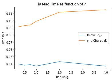
Figure 1: Comparison of our bi-level method with Chu et al. Processing time as a function of the radius (matrices fixed, 1000x10000)

The size of the matrices is, 1000x10000, values between 0 and 1 uniformly sampled. Figure 1 shows that the running time as a function of the radius is at least 2.5 times faster than the actual fastest method, Chu et al.. Note that the running time of the bi-level one is almost not impacted by the radius.

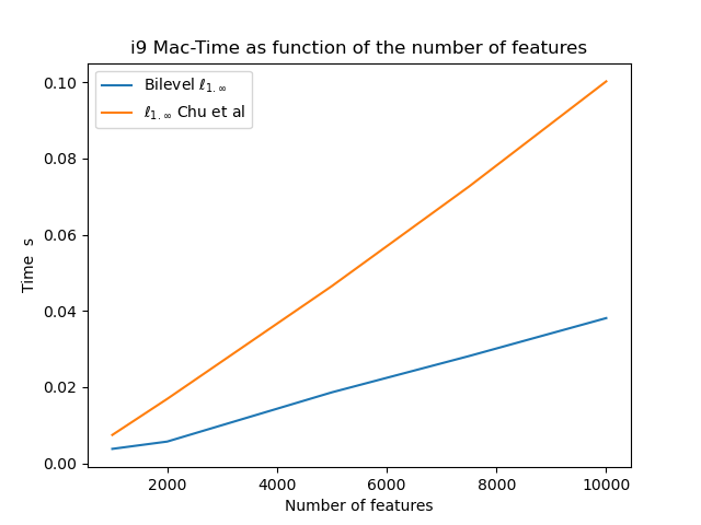
Figure 2: Processing time using C++: our bi-level projection method versus Chu et. al. method. m=1000 and $\eta=1$ fixed .

Figure 2 shows the running time as a function of the matrix size. Here the radius has been fixed to $\eta=1$. The running time of our bilevel method is at least 2.5 faster than that of the actual fastest method when increasing the matrix size both in number of columns and rows. Note that PyTorch c++ extension is 20 times faster than the standard PyTorch implementation.

5.2 Benchmark of Identity Proposition

We generate two artificial biological datasets to benchmark our bi level projection using the $make\_classification$ utility from scikit-learn. We generate $n=1,000$ samples with a number of $m=1000$ features. The first one with 64 (data-64) informative features and the second (data-16) with 16 informative features
We provide the experimental proof of the proposition and the sparsity score in $\%$: number of columns or features set to zero.

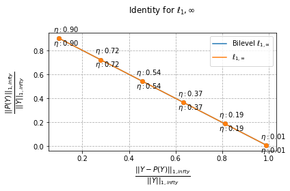
Figure 3: Identity norm comparison of our bi-level $\ell_{1,\infty}$ projection method versus classical.

Fig 3 shows that the two curves ( Bilevel and usual $\ell_{1,\infty}$ projections) and the $\eta$ are parameter are perfectly coincident, and perfectly linear as expected by the identity equations [18].

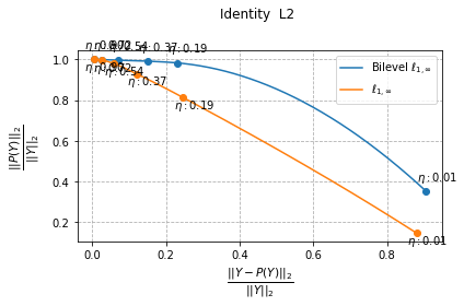
Figure 4: Identity norm $L_{2}$ error comparison of our bi-level projection method versus classical.

Fig 4 shows that $P\ell_{1,\infty}$ has the best $L_{2}$ error, However $L_{2}$ error is not more relevant for our purpose than any other norm.

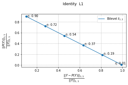
Figure 5: Identity norm our bi-level$\ell_{1,1}$ projection method with L1 norm.

Fig 5 shows that the curve Bilevel $\ell_{1,1}$ is perfectly linear as expected by the identity equation 24.

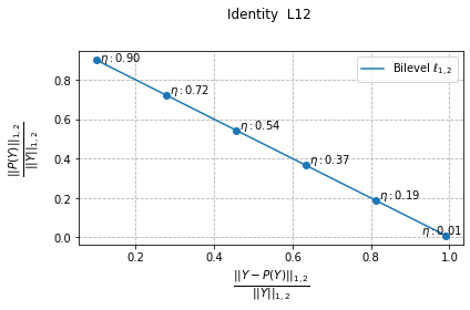
Figure 6: Identity norm, our bi-level $\ell_{1,2}$ projection method.

Fig 6 shows that the curve Bilevel $\ell_{1,2}$ projection satisfies the identity matrix relation.

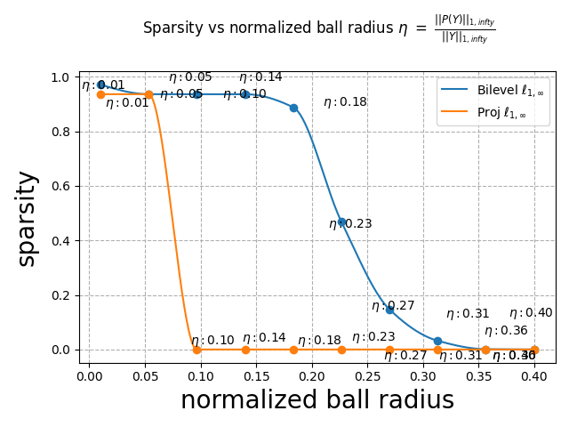
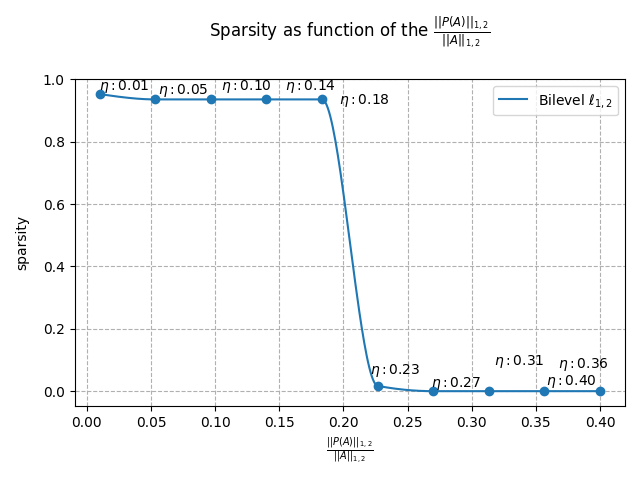
Figure 7: 64 informative features Sparsity Top the Bilevel $\ell_{1,\infty}$, Middle: Bilevel $\ell_{1,1}$, bottom: Bilevel $\ell_{1,2}$ projection

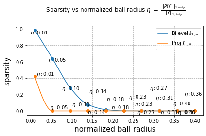
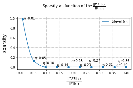
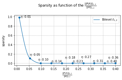
Figure 8: 16 informative features. Sparsity Top the Bilevel $\ell_{1,\infty}$, Middle: Bilevel $\ell_{1,1}$, bottom: Bilevel $\ell_{1,2}$ projection

Cumul Sparsity	bi-level $\ell_{1,\infty}$	bi-level $\ell_{1,1}$	bi-level $\ell_{1,\infty}$	$\ell_{1,\infty}$
datas-64	5.36	4.714	4.705	1.872
data-16	1.99	1.09	1.07	0.419

Table 1: Comparison of Sparsity for two datasets with different informative features

Table 1 shows that our bilevel $\ell_{1,\infty}$ projection outperforms sparsity of bilevel $\ell_{1,1}$ projection and bilevel $\ell_{1,2}$. Although the sparsity curves look very close; Table 1 shows that bilevel $\ell_{1,1}$ projection is slightly more sparse than bilevel $\ell_{1,2}$.

The code is available online

5.3 Experimental results on classification and feature selection using a supervised autoencoder neural network

5.3.1 Supervised Autoencoder (SAE) framework

Autoencoders were introduced within the field of neural networks decades ago, their most efficient application being dimensionality reduction [36, 37]. Autoencoders were used in application ranging from unsupervised deep-clustering [38, 39] to supervised learning adding a classification loss in order to improve classification performance [40, 41]. In this paper, we use the cross entropy as the added classification loss.
Let $X$ be the dataset in $\mathbb{R}^{d}$, and $Y$ the labels in $\{0,\dots,k\}$, with $k$ the number of classes. Let $Z\in\mathbb{R}^{k}$ be the encoded latent vectors, $\widehat{X}$ $\in\mathbb{R}^{d}$ the reconstructed data and $W$ the weights of the neural network. Note that the dimension of the latent space $k$ corresponds to the number of classes.
The goal is to learn the network weights, $W$ minimizing the total loss. In order to sparsify the neural network, we propose to use the different bi-level projection methods as a constraint to enforce sparsity in our model. The global criterion is:

$$\underset{W}{\text{minimize}}\quad\phi(X,Y)\quad\text{ subject to }\quad BP^{1,\infty}(W)\leq\eta$$ (28)

where $\phi(X,Y)=$ $\alpha\psi(X,\widehat{X}))+$ $\mathcal{H}(Y,Z)$. We use the Cross Entropy Loss$\mathcal{H}$ as the added classification loss and the robust Smooth $\ell_{1}$ (Huber) Loss [42] as the reconstruction loss $\psi$. Parameter $\alpha$ is a linear combination factor used to define the final loss. We compute the mask by using the various bilevel projection methods, and we use the double descent algorithm [43, 44] for minimizing the criterion 28. We implemented our SAE method using the PyTorch framework for the model, optimizer, schedulers and loss functions. We use a fully connected neural network with only one hidden layer (dimension 100) and a latent layer of dimension $k=2$ . We chose the ADAM optimizer [45], as the standard optimizer in PyTorch. We used a symmetric linear fully connected network with the encoder comprised of an input layer of $d$ neurons, one hidden layer followed by a ReLU or SiLU activation function.

5.3.2 Experimental accuracy results on autoencoder neural neworks

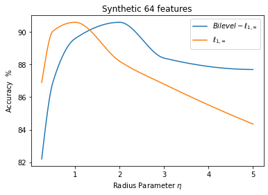
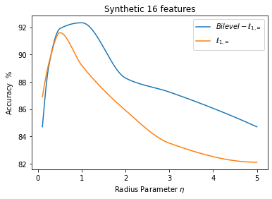
Figure 9: Accuracy as a function of the radius parameter $\eta$; Left, 64 informative features :16 informative features

Figure 9 shows the impact of the radius ($\eta$) on a synthetic dataset using by the bilevel projection. We consider now one of the real dataset from the study of in single-cell CRISPRi screening [46]. This dataset is composed of 779 cells and 10,000 features (genes).

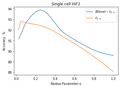
Figure 10: Accuracy as a function of the radius parameter $\eta$; HIF2 dataset

Figure 10 shows the impact of the radius ($\eta$) on HIF2 dataset using by the bilevel projection.

From Tables 2 on synthetic dataset and Table 2 it can be seen that the best accuracy is obtained for $\eta=0.5$ for $\ell_{1,\infty}$ and for $\eta=1.$ for the bilevel $\ell_{1,\infty}$ projection, maximum accuracy of both method are similar. However, sparsity and computation time are better for bilevel $\ell_{1,\infty}$ than for regular $\ell_{1,\infty}$.

Synthetic 64	Baseline	$\ell_{1,\infty}$	bi-level $\ell_{1,\infty}$
Best Radius		1	2.0
Accuracy $\%$	80.3	90.6.6$\pm 1.2$	90.6 $\pm 1.45$

Table 2: Synthetic dataset 64 features. SiLU activation, Accuracy : comparison of $\ell_{1,\infty}$ and bi-level $\ell_{1,\infty}$.

Synthetic 16	Baseline	$\ell_{1,\infty}$	bi-level $\ell_{1,\infty}$
Best Radius		0.5	1.0
Accuracy $\%$	74.6	91.6 $\pm 1.2$	92.36 $\pm 1.45$

Table 3: Synthetic dataset 16 features. SiLU activation, Accuracy : comparison of $\ell_{1,\infty}$ and bi-level $\ell_{1,\infty}$.

Table 2 shows accuracy classification for 64 informative features. The baseline is an implementation that does not process any projection. Compared to the baseline, the SAE using the $\ell_{1,\infty}$ projection improves the accuracy by $10.3\%$.
Table 3 shows that accuracy results for 16 informative features of the bi-level $\ell_{1,\infty}$ and classical $\ell_{1,\infty}$ are similar. Again, compared to the baseline, the SAE using the bilevel $\ell_{1,\infty}$ projection improves the accuracy by $17.7\%$.

Real data HIF2	Baseline	$\ell_{1,\infty}$	bi-level $\ell_{1,\infty}$
Best Radius		0.1	0.25
Accuracy $\%$	84.6	92.68 $\pm 1.2$	93.88 $\pm 1.45$

Table 4: HIF2 SiLU activation, Accuracy : comparison of $\ell_{1,\infty}$ and bi-level $\ell_{1,\infty}$.

Again, on this real dataset, compared to the baseline the SAE using the bilevel $\ell_{1,\infty}$ projection improves the accuracy by $10\%$ similar to the results on the synthetic data-64.

6 Discussion

A first application of our bilevel $\ell_{1,\infty}$ projection is feature selection in biology [46].
Second, our bilevel method can be extended straight forward to tensor and convolutionnal neural networks. Thus, sparsity improves computational cost. Note that the $\ell_{1,1}$ projection was also used in order to sparsify convolutionnal neural networks [47] for green AI. This $\ell_{1,1}$ projection was also used for image compression using autoencoder [48] improving computational cost of new image coding method [37, 49] Our new bilevel $\ell_{1,\infty}$ projection will outperform all other projections in terms of computation cost and sparsity.

7 Conclusion

Although many projection algorithms were proposed for the projection of the $\ell_{1,\infty}$ norm, complexity of these algorithms remain an issue. The worst-case time complexity of these algorithms is $\mathcal{O}\big{(}n\times m\times\log(n\times m)\big{)}$ for a matrix in $\mathbb{R}^{n\times m}$. In order to cope with this complexity issue, we have proposed a new bi-level projection method. The main motivation of our work is the direct independent splitting made by the bi-level optimization, which takes into account the structured sparsity requirement. We showed that the theoretical computational cost of our new bi-level method is only $\mathcal{O}\big{(}n\times m\big{)}$ for a matrix in $\mathbb{R}^{n\times m}$. Experiments on synthetic and real data show that our bi-level method is 2.5 times faster than the actual fastest algorithm provided by Chu et. al.. Sparsity of our bi-level $\ell_{1,\infty}$ projection outperforms other bi-level projections $\ell_{1,1}$ and $\ell_{1,2}$.

References

- [1] Z. He and W. Yu, “Stable feature selection for biomarker discovery,” Computational biology and chemistry, vol. 34, no. 4, pp. 215–225, 2010.
- [2] R. Schwartz, J. Dodge, N. A. Smith, and O. Etzioni, “Green AI,” 2019, preprint arXiv:1907.10597.
- [3] J. M. Alvarez and M. Salzmann, “Learning the number of neurons in deep networks,” in Advances in Neural Information Processing Systems, 2016, pp. 2270–2278.
- [4] S. Han, J. Pool, J. Tran, and W. Dally, “Learning both weights and connections for efficient neural network,” in Advances in neural information processing systems, 2015, pp. 1135–1143.
- [5] A. N. Gomez, I. Zhang, K. Swersky, Y. Gal, and G. E. Hinton, “Learning sparse networks using targeted dropout,” arXiv :1905.13678, 2019.
- [6] N. Srivastava, G. Hinton, A. Krizhevsky, I. Sutskever, and R. Salakhutdinov, “Dropout: a simple way to prevent neural networks from overfitting,” The journal of machine learning research, vol. 15, no. 1, pp. 1929–1958, 2014.
- [7] J. Cavazza, P. Morerio, B. Haeffele, C. Lane, V. Murino, and R. Vidal, “Dropout as a low-rank regularizer for matrix factorization,” in International Conference on Artificial Intelligence and Statistics (AISTATS), 2018, pp. 435–444.
- [8] R. Tibshirani, “Regression shrinkage and selection via the lasso,” Journal of the Royal Statistical Society. Series B (Methodological), pp. 267–288, 1996.
- [9] T. Hastie, R. Tibshirani, and M. Wainwright, “Statistcal learning with sparsity: The lasso and generalizations,” CRC Press, 2015.
- [10] M. Yuan and Y. Lin, “Model selection and estimation in regression with grouped variables,” Journal of the Royal Statistical Society: Series B (Statistical Methodology), vol. 68, no. 1, pp. 49–67, 2006.
- [11] Z. Huang and N. Wang, “Data-driven sparse structure selection for deep neural networks,” in Proceedings of the European Conference on Computer Vision (ECCV), 2018, pp. 304–320.
- [12] J. Yoon and S. J. Hwang, “Combined group and exclusive sparsity for deep neural networks,” in Proceedings of the 34th International Conference on Machine Learning-Volume 70. JMLR. org, 2017, pp. 3958–3966.
- [13] S. Scardapane, D. Comminiello, A. Hussain, and A. Uncini, “Group sparse regularization for deep neural networks,” Neurocomputing, vol. 241, pp. 81–89, 2017.
- [14] N. Simon, J. Friedman, T. Hastie, and R. Tibshirani, “A sparse-group lasso,” Journal of Computational and Graphical Statistics, vol. 22, no. 2, pp. 231–245, 2013.
- [15] I. Yasutoshi, F. Yasuhiro, and K. Hisashi, “Fast sparse group lasso,” in Advances in Neural Information Processing Systems, vol. 32. Curran Associates, Inc., 2019.
- [16] J. Friedman, T. Hastie, and R. Tibshirani, “Regularization path for generalized linear models via coordinate descent,” Journal of Statistical Software, vol. 33, pp. 1–122, 2010.
- [17] J. Mairal and B. Yu, “Complexity analysis of the lasso regularization path,” in Proceedings of the 29th International Conference on Machine Learning (ICML-12), 2012, pp. 353–360.
- [18] G. Chierchia, N. Pustelnik, J. C. Pesquet, and B. Pesquet-Popescu, “Epigraphical projection and proximal tools for solving constrained convex optimization problems,” Signal, Image and Video Processing, 2015.
- [19] M. Barlaud, W. Belhajali, P. Combettes, and L. Fillatre, “Classification and regression using an outer approximation projection-gradient method,” vol. 65, no. 17, 2017, pp. 4635–4643.
- [20] L. Condat, “Fast projection onto the simplex and the l1 ball,” Mathematical Programming Series A, vol. 158, no. 1, pp. 575–585, 2016.
- [21] G. Perez, M. Barlaud, L. Fillatre, and J.-C. Régin, “A filtered bucket-clustering method for projection onto the simplex and the -ball,” Mathematical Programming, May 2019.
- [22] A. Quattoni, X. Carreras, M. Collins, and T. Darrell, “An efficient projection for regularization,” in Proceedings of the 26th Annual International Conference on Machine Learning, 2009, pp. 857–864.
- [23] B. Bejar, I. Dokmanić, and R. Vidal, “The fastest prox in the West,” IEEE transactions on pattern analysis and machine intelligence, vol. 44, no. 7, pp. 3858–3869, 2021.
- [24] G. Chau, B. Wohlberg, and P. Rodriguez, “Efficient projection onto the mixed-norm ball using a newton root search method,” SIAM Journal on Imaging Sciences, vol. 12, no. 1, pp. 604–623, 2019.
- [25] D. Chu, C. Zhang, S. Sun, and Q. Tao, “Semismooth newton algorithm for efficient projections onto -norm ball,” in International Conference on Machine Learning, 2020, pp. 1974–1983.
- [26] J. J. Moreau, “Fonctions convexes duales et points proximaux dans un espace hilbertien,” Comptes Rendus de l’Académie des Sciences de Paris, vol. A255, no. 22, pp. 2897–2899, Nov 1962.
- [27] H. H. Bauschke and P. L. Combettes, Convex Analysis and Monotone Operator Theory in Hilbert Spaces, 2nd ed. New York: Springer, 2017.
- [28] P. L. Combettes and J.-C. Pesquet, “Proximal splitting methods in signal processing,” in Fixed-point algorithms for inverse problems in science and engineering. Springer, 2011, pp. 185–212.
- [29] L. Condat, D. Kitahara, A. Contreras, and A. Hirabayashi, “Proximal splitting algorithms for convex optimization: A tour of recent advances, with new twists,” SIAM Review, vol. 65, no. 2, pp. 375–435, May 2023.
- [30] G. Perez, L. Condat, and M. Barlaud, “Near-linear time projection onto the l1,infty ball application to sparse autoencoders.” arXiv: 2307.09836, 2023.
- [31] A. Sinha, P. Malo, and K. Deb, “A review on bilevel optimization: From classical to evolutionary approaches and applications,” IEEE Transactions on Evolutionary Computation, vol. 22, no. 2, pp. 276–295, 2018.
- [32] K. Bennett, J. Hu, X. Ji, G. Kunapuli, and J.-S. Pang, “Model selection via bilevel optimization,” IEEE International Conference on Neural Networks - Conference Proceedings, 2006.
- [33] P. C. Hansen and D. P. O’Leary, “The use of the l-curve in the regularization of discrete ill-posed problems,” SIAM Journal on Scientific Computing, vol. 14, 1993.
- [34] J. Moreau, “Proximité et dualité dans un espace hilbertien,” Bull. Soc.Math. France., 93, pp. 273–299, 1965.
- [35] N. Parikh and S. Boyd, “Proximal algorithms,” Foundations and Trends® in Optimization, 2014.
- [36] I. Goodfellow, Y. Bengio, and A. Courville, Deep learning. MIT press, 2016, vol. 1.
- [37] L. Theis, W. Shi, A. Cunningham, and F. Huszár, “Lossy image compression with compressive autoencoders,” ICLR Conference Toulon, 2017.
- [38] D. Kingma and M. Welling, “Auto-encoding variational bayes,” International Conference on Learning Representation, 2014.
- [39] J. Snoek, R. Adams, and H. Larochelle, “On nonparametric guidance for learning autoencoder representations,” in Artificial Intelligence and Statistics. PMLR, 2012, pp. 1073–1080.
- [40] L. Le, A. Patterson, and M. White, “Supervised autoencoders: Improving generalization performance with unsupervised regularizers,” Advances in Neural Information Processing Systems, 2018.
- [41] M. Barlaud and F. Guyard, “Learning a sparse generative non-parametric supervised autoencoder,” Proceedings of the International Conference on Acoustics, Speech and Signal Processing, Toronto, Canada, June 2021.
- [42] P. J. Huber, Robust statistics. Wiley, New York, 1981.
- [43] J. Frankle and M. Carbin, “The lottery ticket hypothesis: Finding sparse, trainable neural networks,” arXiv preprint arXiv:1803.03635, 2018.
- [44] H. Zhou, J. Lan, R. Liu, and J. Yosinski, “Deconstructing lottery tickets: Zeros, signs, and the supermask,” in Advances in Neural Information Processing Systems 32, 2019, pp. 3597–3607.
- [45] D. Kingma and J. Ba, “a method for stochastic optimization.” International Conference on Learning Representations, pp. 1–13, 2015.
- [46] M. Truchi, C. Lacoux, C. Gille, J. Fassy, V. Magnone, R. Lopes Goncalves, C. Girard-Riboulleau, I. Manosalva-Pena, M. Gautier-Isola, K. Lebrigand, P. Barbry, S. Spicuglia, G. Vassaux, R. Rezzonico, M. Barlaud, and B. Mari, “Detecting subtle transcriptomic perturbations induced by lncrnas knock-down in single-cell crispri screening using a new sparse supervised autoencoder neural network,” Frontiers in Bioinformatics, 2024.
- [47] M. Barlaud and F. Guyard, “Learning sparse deep neural networks using efficient structured projections on convex constraints for green ai,” International Conference on Pattern Recognition, Milan, pp. 1566–1573, 2020.
- [48] G. Cyprien, F. Guyard, M. Antonini, and M. Barlaud, “Learning sparse autoencoders for green ai image coding,” Proceedings of the International Conference on Acoustics, Speech and Signal Processing, Rhodes, Greece, June 2023.
- [49] J. Ascenso, E. Alshina, and T. Ebrahimi, “The jpeg ai standard: Providing efficient human and machine visual data consumption,” IEEE MultiMedia, vol. 30, no. 1, pp. 100–111, 2023.