A martingale-type of characterisation of the Gaussian free field and fractional Gaussian free fields

Abstract.

We establish a martingale-type characterisations for the continuum Gaussian free field (GFF) and for fractional Gaussian free fields (FGFs), using their connection to the stochastic heat equation and to fractional stochastic heat equations.

The main theorem on the GFF generalizes previous results of similar flavour and the characterisation theorems on the FGFs are new. The proof strategy is to link the resampling dynamics coming from a martingale-type of decomposition property to the stationary dynamics of the desired field, i.e. to the (fractional) stochastic heat equation.

1. Introduction

We prove a martingale-type characterisation results for the continuum Gaussian free field (GFF) and for fractional Gaussian free fields (FGFs), using their connection to the stochastic heat equation and to fractional stochastic heat equations.

Such characterisation theorems are well-known in the case of Brownian motion - e.g. the identification as the only continuous process with independent stationary increments or as the only continuous semimartingale with linear quadratic variation - and they help to explain the central role of Brownian motion in probability theory. One could ask if similar characterisations for the $d$-dimensional continuum Gaussian free field and its fractional counterparts might also bring some insight into its universality - for example the GFF is both the proven and the conjectured scaling limit of several natural discrete height functions [Nad97, Ken01, RV07, BLR20]. Next to this, characterisation theorems also help to understand better which properties are central to the underlying object.

1.1. The case of the Gaussian free field

The Dirichlet boundary condition continuum Gaussian Free Field (abbreviated GFF), which can be viewed as a generalization to higher dimensions of the Brownian Motion, is defined as follows.

Definition 1.1.

The GFF on a bounded regular domain $D$ is the centred Gaussian process $(h^{D},f)_{\_}{f\in C_{\_}c^{\infty}(D)}$ whose covariance is

$$\mathbb{E}[(h^{D},f)(h^{D},g)]=\int_{\_}D\int_{\_}Df(x)G_{\_}D(x,y)g(y)dxdy.$$

Here, a regular domain is any connected open subset of $\mathbb{R}^{d}$ with finitely many boundary components, such that for every $x\in\partial D$ the frontier of a domain $D$, the Brownian motion $B_{\_}t$ starting from $x$ satisfies $\inf\{t>0\leavevmode\nobreak\ :\leavevmode\nobreak\ B_{\_}t\in D^{c}\}=0$ almost surely; this guarantees that the Green’s function is well defined and positive definite. Further boundedness guarantees that the Green’s integral operator is compact.

In [BPR20] the authors showed that for $d=2$, the GFF is the only conformally invariant field satisfying a domain Markov property under some continuity and moments assumptions; these moment assumptions were then lowered in [BPR21]. Further, in [AP22], the authors proved a characterisation of the GFF in $d\geq 2$, which heuristically corresponds to the stationary independent increments property. The proof there is simple, but is tailored to balls, or other domains with symmetry.

The first contribution paper is to show a martingale-type of characterisation for the continuum GFF, which also works in a more general geometric setting then the earlier works [BPR20, BPR21, AP22], e.g. in multiply connected domains. We prove that essentially the GFF is characterized by the following martingale-type decomposition property - in any ball the field can be written as a sum of a harmonic function and a zero mean, zero-boundary field with certain scaling. This is considerably weaker than the domain Markov property assumed in [BPR20, AP22]. A more precise statement of this decomposition goes as follows:

Definition 1.2 (Martingale-type decomposition).

We say that a random distribution $h^{D}\in\mathcal{S}_{\_}D$ admits the martingale type decomposition (abbreviated MTD) if for any ball $B:=B(x,\varepsilon)\subset D$ we have the decomposition

$$h^{D}=\tilde{h}^{B}+\varphi_{\_}D^{B},$$

where $\varphi_{\_}D^{B}$ belongs to $\mathcal{S}_{\_}D$ and corresponds to integrating with respect to an harmonic function when restricted to $B$ ; and $\tilde{h}^{B}$ belongs to $\mathcal{S}_{\_}B$ and satisfies the following conditions, where $\mathchoice{{T\,\smash{\vrule height=5.46666pt,depth=2.00412pt}}_{\,D^{\prime}}}{{T\,\smash{\vrule height=5.46666pt,depth=2.00412pt}}_{\,D^{\prime}}}{{T\,\smash{\vrule height=3.82666pt,depth=1.53944pt}}_{\,D^{\prime}}}{{T\,\smash{\vrule height=2.73332pt,depth=1.53944pt}}_{\,D^{\prime}}}$ is the restriction of a distribution $T$ to the subdomain $D^{\prime}$..

1. The martingale property: for any $f\in C^{\infty}_{\_}c(D)$

   $$\mathbb{E}\left[(\tilde{h}^{B},f)\leavevmode\nobreak\ |\leavevmode\nobreak\ \sigma\big{(}\mathchoice{{(h^{D})\,\smash{\vrule height=7.08624pt,depth=2.12502pt}}_{\,D\setminus B}}{{(h^{D})\,\smash{\vrule height=7.08624pt,depth=2.12502pt}}_{\,D\setminus B}}{{(h^{D})\,\smash{\vrule height=4.98222pt,depth=1.4875pt}}_{\,D\setminus B}}{{(h^{D})\,\smash{\vrule height=3.87111pt,depth=1.43933pt}}_{\,D\setminus B}}\big{)}\right]=0.$$

2. A condition on the second moments of the increments: the squared increment is deterministic, i.e. for any $f\in C^{\infty}_{\_}c(D)$

   $$\mathbb{E}\left[(\tilde{h}^{B},f)^{2}|\leavevmode\nobreak\ \mathchoice{{(h^{D})\,\smash{\vrule height=7.08624pt,depth=2.12502pt}}_{\,D\setminus B}}{{(h^{D})\,\smash{\vrule height=7.08624pt,depth=2.12502pt}}_{\,D\setminus B}}{{(h^{D})\,\smash{\vrule height=4.98222pt,depth=1.4875pt}}_{\,D\setminus B}}{{(h^{D})\,\smash{\vrule height=3.87111pt,depth=1.43933pt}}_{\,D\setminus B}}\right]=\mathbb{E}\left[(\tilde{h}^{B},f)^{2}\right]$$

   and we have weak scaling: for some $C>0$ and some positive bounded measurable function $a:D\to(0,\infty)$

   $$\mathbb{E}\left[(\tilde{h}^{B},f)^{2}\leavevmode\nobreak\ |\leavevmode\nobreak\ \mathchoice{{(h^{D})\,\smash{\vrule height=7.08624pt,depth=2.12502pt}}_{\,D\setminus B}}{{(h^{D})\,\smash{\vrule height=7.08624pt,depth=2.12502pt}}_{\,D\setminus B}}{{(h^{D})\,\smash{\vrule height=4.98222pt,depth=1.4875pt}}_{\,D\setminus B}}{{(h^{D})\,\smash{\vrule height=3.87111pt,depth=1.43933pt}}_{\,D\setminus B}}\right]\leq C\sup_{\_}{z\in D}|f(z)|^{2}\varepsilon^{2+d}; \frac{\mathbb{E}\left[(\tilde{h}^{B},f)^{2}\leavevmode\nobreak\ |\leavevmode\nobreak\ \mathchoice{{(h^{D})\,\smash{\vrule height=7.08624pt,depth=2.12502pt}}_{\,D\setminus B}}{{(h^{D})\,\smash{\vrule height=7.08624pt,depth=2.12502pt}}_{\,D\setminus B}}{{(h^{D})\,\smash{\vrule height=4.98222pt,depth=1.4875pt}}_{\,D\setminus B}}{{(h^{D})\,\smash{\vrule height=3.87111pt,depth=1.43933pt}}_{\,D\setminus B}}\right]}{\varepsilon^{2+d}}\to_{\_}{\varepsilon\to 0}a^{2}(x)f^{2}(x)$$

   where the convergence is uniform on compacts.

3. The field $\tilde{h}^{B}$ satisfies zero boundary conditions in the sense defined just below.

We will in fact have to add a weak condition on the fourth moment of $\tilde{h}^{B}$ too, though possibly this can be relaxed further. Also, both in this definition and in the theorem below we have to define what it means for a distribution to have zero boundary conditions. We follow here [AP22]:

Definition 1.3 (Zero boundary conditions).

We say that a random distribution $h^{D}\in\mathcal{S}_{\_}D$ satisfies zero boundary conditions in the $L^{2}$ sense if the following holds.

Consider a sequence $(g_{\_}n)_{\_}{n\geq 1}$ of positive and of uniformly bounded mass functions of $C^{\infty}_{\_}c(D)$ such that $\sup_{\_}{n\geq 1}\sup_{\_}{r>0}\sup_{\_}{x,y\in D_{\_}r}|g_{\_}n(x)/g_{\_}n(y)|<\infty$ where $D_{\_}r:=\{z\in D\,:\,d(z,\partial D)=r\}$, and for every compact $K\subset D$ it holds that $K\cap\emph{supp}(g_{\_}n)=\emptyset$ for $n$ large enough. Then we have that $\mathbb{E}[(h^{D},g_{\_}n)^{2}]\mapsto 0$ as $n\mapsto\infty$.

The characterisation theorem can be now stated:

Theorem 1.4.

Let $d\geq 2$ and $D$ be a regular domain of $\mathbb{R}^{d}$. Suppose that a random distribution $h^{D}\in\mathcal{S}_{\_}D$ satisfies the following properties

• Martingale-type decomposition : as in Definition 1.2, and satisfying in addition for some $C_{\_}x>0$ that is bounded on compacts

  $$\mathbb{E}\left[(\tilde{h}^{B(x,\varepsilon)},f)^{4}\right]\leq C_{\_}x^{4}\sup_{\_}{z\in D}|f(z)|^{4}\varepsilon^{2(2+d)}.$$

• Uniformly bounded 4th moments : there is some $C_{\_}0=C(D)>0$ such that for any $f\in C_{\_}c^{\infty}(D)$, we have

  $$\mathbb{E}[(\tilde{h}^{B},f)^{4}]\leq C_{\_}0^{2}\sup_{\_}{z\in D}|f(z)|^{4}.$$

• Zero boundary conditions as in the Definition 1.3.

Then there exists $c\geq 0$ such that $c\,h^{D}$ is a GFF.

Remark 1.5.

Compared to [AP22] (and [BPR20]) the main difference is the weakening of the domain Markov property. Indeed, in these articles the field was decomposed in every ball as a sum of a harmonic function and an independent field that was a rescaled version of the original field. Here we do not demand independence of the decomposition nor ask much from the law of the non-harmonic part, other than being centred, with zero boundary and satisfying some scaling. The latter is necessary, as otherwise white noise would satisfy the conditions too.

We also allow for a certain possible non-homogeneity with $a$ non-constant in the MTD; yet one should emphasise that our theorem shows that for all the fields that do satisfy MTD with our additional conditions, the function $a$ ends up being constant.

Further notice that the 4th moment condition in A and B is asking more than [AP22, BPR21] in terms of moments: indeed, the uniformity we ask here was not part of their assumptions. One could get away with less, e.g. by assuming a uniform bound only for certain symmetric mollifiers; this would already very simply follow from the stronger Markov decomposition in [AP22, BPR21] combined with just the finiteness of fourth moments.

Finally, a simple sanity check is that the GFF itself does satisfy the conditions of the theorem.

The proof strategy is as follows:

• the martingale-type decomposition gives us a natural way to resample the field inside balls and using a Poisson point process of these resamplings on randomly located balls we construct a stochastic dynamics on random fields, whose marginal law is equal to the initial field for every time $t>0$ (Definition 2.13);

• we show that this dynamics when we resample in smaller and smaller balls and with higher and higher frequency converges to the stochastic heat equation (Theorem 2.15);

• to conclude we use the fact that the unique stationary solution of the stochastic heat equation is the Gaussian free field.

In the case where the function $a$ is constant, i.e. we assume some homogeneity in space, we can follow this sketch rather precisely and interestingly - in contrast to [AP22, BPR20] we don’t need an extra step to identify the covariance kernel. In the case $a$ non-constant, we still need to make use of a separate step to identify the covariance as the Green’s kernel, but that is standard by now.

This strategy for proving the characterisation theorem is quite robust and would also work for Riemann surfaces with boundary, answering partly Question 6.6 of [BPR20]. Here we exemplify the generality by using the same strategy to prove a characterisation theorem for the fractional Gaussian fields, e.g. like the fractional Brownian motion, and answering Question 6.5 of [BPR20] for a range of parameters.

1.2. The case of fractional Gaussian fields

Fractional Gaussian free fields $\text{FGF}_{\_}\alpha(D)$ can be defined as follows [LPG⁺20]:

Definition 1.6.

For $\alpha>0$, the $\text{FGF}_{\_}\alpha(D)$ on a bounded domain with smooth boundary is the centred Gaussian process $(h^{D}_{\_}\alpha,f)_{\_}{f\in C^{\infty}_{\_}c(D)}$ whose covariance is

$$\mathbb{E}[(h^{D}_{\_}\alpha,f)(h^{D}_{\_}\alpha,g)]=\int_{\_}D\int_{\_}Df(x)G_{\_}D^{\alpha}(x,y)g(y)dxdy,$$

where $G_{\_}D^{\alpha}$ is the fractional Green function associated to the fractional laplacian $(-\Delta)^{\alpha}$ on $D$.

The operator $(-\Delta)^{\alpha}u(z)$ here is the Riesz fractional Laplacian given by

(1) $$(-\Delta)^{\alpha}u(z)=\lim_{\_}{\varepsilon\mapsto 0}\int_{\_}{\mathbb{R}^{d}-B(z,\varepsilon)}\frac{u(z)-u(y)}{|z-y|^{d+2\alpha}}dy,$$

where we extended the values of $u$ outside of $D$ by $0$ (see e.g. [LSSW14, BBK⁺09]). It is known that the fractional Green function $G_{\_}D^{\alpha}$ exists; in the case $D=\mathbb{B}$ where $\mathbb{B}$ is the unit ball, it can be explicitly computed, see Section 3.1. The case $\alpha=1$ corresponds to the Gaussian free field, in the case $d=1$ and $\alpha\in(1/2,3/2)$ we obtain the fractional Brownian bridges with the Hurst parameter $H=\alpha-d/2$, see [LPG⁺20]. We will concentrate on the range $\alpha\in(0,1)$ where the Riesz laplacian is the generator of a $2\alpha-$stable Lévy process.

In the fractional case the characterisation theorems have not been explored too much; even in the case of fractional Brownian motion characterisation theorems are relatively new - [MV11, HNS09]. Given the recent interest in processes related to the fractional Laplacian - e.g. [LSSW14, CS24, GP24] but also [Gar24] - it might be good to see what additional difficulties they might pose from the point of view of characterisations in the spirit of [BPR20, AP22].

In essence the characterisation of the GFF obtained in Theorem 1.4 generalizes nicely to fractional Gaussian free fields $\text{FGF}_{\_}\alpha(D)$ in the regime $0<\alpha<1$: the fractional Gaussian free field is characterised by having a martingale-type of decomposition on each ball: the field inside is given by a $\alpha-$harmonic function plus a zero mean, zero boundary field as before.

Definition 1.7.

Let $d\geq 2$ and $\alpha\in(0,1)$. We say that a random distribution $h^{D}\in\mathcal{S}_{\_}D$ admits the (fractional) martingale type decomposition (abbreviated FMTD) if for any ball $B:=B(x,\varepsilon)\subset D$ we have the decomposition

$$h^{D}=\tilde{h}^{B}+\varphi_{\_}D^{B},$$

where $\varphi_{\_}D^{B}$ belongs to $\mathcal{S}_{\_}D$, corresponds to integrating with respect to an $\alpha$-harmonic function (ie $(-\Delta)^{\alpha}\varphi_{\_}D^{B}=0$, see below for more details on the fractional laplacian) when restricted to $B$ and $\tilde{h}^{B}$ belongs to $\mathcal{S}_{\_}B$ and satisfies the following conditions.

1. The martingale property: for any $f\in C^{\infty}_{\_}c(D)$

   $$\mathbb{E}\left[(\tilde{h}^{B},f)\leavevmode\nobreak\ |\leavevmode\nobreak\ \sigma\big{(}\mathchoice{{(h^{D})\,\smash{\vrule height=7.08624pt,depth=2.12502pt}}_{\,D\setminus B}}{{(h^{D})\,\smash{\vrule height=7.08624pt,depth=2.12502pt}}_{\,D\setminus B}}{{(h^{D})\,\smash{\vrule height=4.98222pt,depth=1.4875pt}}_{\,D\setminus B}}{{(h^{D})\,\smash{\vrule height=3.87111pt,depth=1.43933pt}}_{\,D\setminus B}}\big{)}\right]=0.$$

2. A condition on the second moments of the increments: the squared increment is deterministic, i.e. for any $f\in C^{\infty}_{\_}c(D)$

   $$\mathbb{E}\left[(\tilde{h}^{B},f)^{2}|\leavevmode\nobreak\ \mathchoice{{(h^{D})\,\smash{\vrule height=7.08624pt,depth=2.12502pt}}_{\,D\setminus B}}{{(h^{D})\,\smash{\vrule height=7.08624pt,depth=2.12502pt}}_{\,D\setminus B}}{{(h^{D})\,\smash{\vrule height=4.98222pt,depth=1.4875pt}}_{\,D\setminus B}}{{(h^{D})\,\smash{\vrule height=3.87111pt,depth=1.43933pt}}_{\,D\setminus B}}\right]=\mathbb{E}\left[(\tilde{h}^{B},f)^{2}\right]$$

   and we have weak scaling: for some $C>0$

   $$\mathbb{E}\left[(\tilde{h}^{B},f)^{2}\leavevmode\nobreak\ |\leavevmode\nobreak\ \mathchoice{{(h^{D})\,\smash{\vrule height=7.08624pt,depth=2.12502pt}}_{\,D\setminus B}}{{(h^{D})\,\smash{\vrule height=7.08624pt,depth=2.12502pt}}_{\,D\setminus B}}{{(h^{D})\,\smash{\vrule height=4.98222pt,depth=1.4875pt}}_{\,D\setminus B}}{{(h^{D})\,\smash{\vrule height=3.87111pt,depth=1.43933pt}}_{\,D\setminus B}}\right]\leq C\sup_{\_}{z\in D}|f(z)|^{2}\varepsilon^{2\alpha+d}; \frac{\mathbb{E}\left[(\tilde{h}^{B},f)^{2}\leavevmode\nobreak\ |\leavevmode\nobreak\ \mathchoice{{(h^{D})\,\smash{\vrule height=7.08624pt,depth=2.12502pt}}_{\,D\setminus B}}{{(h^{D})\,\smash{\vrule height=7.08624pt,depth=2.12502pt}}_{\,D\setminus B}}{{(h^{D})\,\smash{\vrule height=4.98222pt,depth=1.4875pt}}_{\,D\setminus B}}{{(h^{D})\,\smash{\vrule height=3.87111pt,depth=1.43933pt}}_{\,D\setminus B}}\right]}{\varepsilon^{2+d}}\to_{\_}{\varepsilon\to 0}f^{2}(x)$$

   where the convergence is uniform on compacts.

3. The field $\tilde{h}^{B}$ satisfies zero boundary conditions in the sense of Lemma 1.3.

Remark 1.8.

Notice that we have given up here the potential local inhomogenity allowed by $a:D\to[0,\infty)$ and normalized it to be $1$. In the case of the GFF - as we saw in Remark 1.5 - there were in the end no fields with $a$ non-constant anyways, and it does simplify our life as we can skip the step of determining the covariance, which would require a bit more potential theory of the fractional laplacian.

There is one key difference from the GFF case stemming from the fact that in general the fractional Laplacian is non-local. Namely, for $\alpha\in(0,1)$ there is no localised mean-value property for $\alpha$-harmonic functions, i.e. for an $\alpha-$harmonic function $f$ we cannot express $f(z)$ by averaging $f$ against some smooth function in any neighbourhood of $z$. Indeed, the $\alpha-$mean kernel is both non-local and non-smooth, as can be seen from the exact expression in Section 3.1. As our fields are a priori distribution valued in the range of interest, this causes some annoyances and one would need to ask for more regularity - basically that integrating the field against the mean-value kernel is well defined. As adding just this as a condition didn’t feel very natural, we opted to further strengthen the martingale-type of property as well - we assume that the $\alpha-$harmonic function in any ball is given by the $\alpha-$Poisson extension of the field outside the ball (in the GFF case this is obtained as a consequence).

Theorem 1.9.

Let $\alpha\in(0,1)$. Suppose that a random distribution $h^{D}\in\mathcal{S}_{\_}D$ has the following property

• FMTD : as in Definition 1.7, and satisfying in addition for some $C>0$

  $$\mathbb{E}\left[(\tilde{h}^{B},f)^{4}\right]\leq C^{4}\sup_{\_}{z\in B}|f(z)|^{4}\varepsilon^{2(2\alpha+d)}.$$

  We further assume that for all balls $B\subset D$ we can evaluate $h^{D}$ against the fractional Poisson kernel $P_{\_}B^{\alpha}(z,\cdot)$ , and moreover we have

  $$(h^{D},P^{\alpha}_{\_}{B}(z,\cdot))=\varphi_{\_}D^{B}(z).$$

• Uniformly bounded 4th moments : there exists a constant $C_{\_}0>0$ such that for any $f\in C^{\infty}_{\_}c(D)$, we have

  $$\mathbb{E}[(h^{D},f)^{4}]\leq C_{\_}0^{2}\sup_{\_}{z\in D}|f(z)|^{4}.$$

• Zero boundary conditions as in the Definition 1.3.

Then there exists $c\geq 0$ such that $c\,h^{D}$ is a $\text{FGF}_{\_}\alpha(D)$.

Remark 1.10.

Notice that as $h^{B}$ is supported in $B$, the final part in condition A’ can also be written as $(\varphi_{\_}D^{B},P^{\alpha}_{\_}{B}(z,\cdot))=\varphi_{\_}D^{B}(z)$.

The fact that the fractional Gaussian free field itself satisfies these conditions can be again checked explicitly, for the zero boundary conditions one can use the estimates in [CS98, Thm 1.1].

As mentioned earlier, the proof of the above theorem stays really pretty much the same. There are only some minor simplifications due to the restated martingale decomposition, and some modifications when proving approximations of $(-\Delta)^{\alpha}$, both detailed in the section about the fractional case. Due to the assumption that the local in-homogeneity $a$ is constant, we can skip the step of determining the covariance altogether.

2. The case of the GFF

In this section we prove the martingale-type of characterisation for the GFF, i.e. Theorem 1.4. In Section 2.1 we start with preliminaries on the stochastic heat equation and then deal with some simple properties of the field $h^{D}$, culminating in the determination of the covariance kernel needed in the case where $a$ is not constant. The second half of this section follows closely [AP22] and is kept short.

Thereafter in Section 2.2 we define the approximate resampling dynamics and state the convergence theorem for this dynamics; we conclude Theorem 1.4 modulo this convergence. Next, in Section 2.3 we identify an approximation of the Laplacian related to our resampling property. In Section 2.4 we identify the relevant martingales and argue that they converge.

Finally in Section 2.5 we obtain the convergence of the original dynamics, concluding the whole proof in the case of the GFF.

2.1. Preliminaries

2.1.1. Preliminaries on the stochastic heat equation

We gather here the definition and some main properties of the additive stochastic heat equation, see e.g. [Wal86] for more details.

Definition 2.1.

Let $d\geq 2$, $D$ a bounded regular domain of $\mathbb{R}^{d}$, and $(\Omega,\mathcal{F},(\mathcal{F}_{\_}t)_{\_}{t\geq 0},\mathbb{P})$ a filtered probability space. The $a$-SHE on $D$ is the SPDE,

(2) $$\begin{cases}&\partial_{\_}tu-\Delta u=a\,\dot{W}\\ &u(0,x)=u_{\_}0(x),\qquad x\in D\\ &u(t,x)=0,\qquad x\in\partial D,\leavevmode\nobreak\ t\geq 0\end{cases}$$

where $\dot{W}$ is a space-time white noise, $a$ is a measurable bounded positive function such that $a\dot{W}$ is a centered Gaussian process defined on Borel subsets of $\mathbb{R}^{+}\times\mathbb{R}^{d}$ whose covariance is $\text{Cov}(a\dot{W}(A),a\dot{W}(B))=\int_{\_}{A\cap B}a^{2}(x)dx$. Further, $u_{\_}0\in\mathcal{F}_{\_}0$ is the initial condition and the zero boundary conditions are to be interpreted in the sense of Definition 1.3.

A mild solution $u$ to (2) is defined as the stochastic process $(u_{\_}t)_{\_}{t\geq 0}$ on $(\Omega,\mathcal{F})$ taking values in the space of distributions $\mathcal{S}_{\_}D$ and such that almost surely for every $t\geq 0$ and $f\in C^{\infty}_{\_}c(D)$

(3) $$(u_{\_}t,f):=\int_{\_}Du_{\_}0(x)\left(\int_{\_}DH_{\_}D(t,x,y)f(y)dy\right)dx+\int_{\_}0^{t}\int_{\_}D\left(\int_{\_}DH_{\_}D(t-s,x,y)a(y)f(y)dy\right)W(dx,ds),$$

where $H_{\_}D$ is the fundamental solution of (2) (also called Green function of the heat kernel) on $D$ and can be expressed by

(4) $$H_{\_}D(t,x,y)=\sum_{\_}{n\in\mathbb{N}}e^{-\mu_{\_}nt}f_{\_}n(x)f_{\_}n(y),$$

where we recall $(f_{\_}n)_{\_}{n\geq 1}$ are an ON basis of $L^{2}(D)$ given by the smooth zero boundary eigenfunctions of the Laplacian, with related eigenvalues $-\Delta f_{\_}n=\mu_{\_}nf_{\_}n$; this is guaranteed by the fact that the domain is bounded and regular, as then the Green’s operator is compact.

Here in the first term of the sum we recognize the solution to the deterministic homogeneous PDE associated to (2), i.e. the heat equation, and the second term is the solution to (2) with $u_{\_}0=0$.

As the stochastic heat equation is a linear parabolic SPDE, the theory of the long-time behaviour of its solutions is well-understood and in particular we have the following proposition, see also e.g. [LS20]

Proposition 2.2 (Existence and uniqueness of stationary solutions).

There is a unique stationary solution to the $a-SHE$, i.e. a unique solution $(u_{\_}t)_{\_}{t\geq 0}$ with $u_{\_}t$ having the same law for all $t\geq 0$ and satisfying zero boundary conditions. Moreover the law of this solution is Gaussian.

In the case $a$ equal to constant, the covariance kernel is very simple and given by

$$\mathbb{E}(u_{\_}t(x)u_{\_}s(y))=\sum_{\_}{n\geq 1}\frac{1}{2\mu_{\_}n}\exp(-\mu_{\_}n|s-t|)f_{\_}n(x)f_{\_}n(y).$$

One way to characterise SPDEs is via the related martingale problem. In the concrete case of the SHE one can even be more precise. See Appendix A for the proof of the following classical result.

Proposition 2.3.

The unique solution to (2) as defined by (3) can be characterized as an element of $\mathcal{S}_{\_}D$ with the infinite sum

$$u_{\_}t:=\sum_{\_}{n=0}^{\infty}A_{\_}n(t)f_{\_}n,$$

where the random variables $A_{\_}n(t)$ are Ornstein-Uhlenbeck processes with parameter $\mu_{\_}n$, ie solutions to the Itô SDEs

(5) $$dX_{\_}t=-\mu_{\_}nX_{\_}td_{\_}t+dB^{n}_{\_}t,$$

with zero initial condition and the $B_{\_}t^{n}$ are Brownian motions of covariation given by $\langle B_{\_}t^{n},B_{\_}t^{m}\rangle=t\langle af_{\_}n\leavevmode\nobreak\ |\leavevmode\nobreak\ af_{\_}m\rangle$. Also, the initial conditions takes the form $\langle u_{\_}0\leavevmode\nobreak\ |\leavevmode\nobreak\ f_{\_}n\rangle=A_{\_}n(t)$.

In fact, using the unique stationary law of Ornstein-Uhlenbeck processes, one can also deduce Proposition 2.2 from Proposition 2.3.
We will use the following corollary:

Corollary 2.4.

Let $(h_{\_}t)_{\_}{t\geq 1}$ be a distribution valued process. Suppose for all $f\in C_{\_}c^{\infty}(D)$ we have that

$$(M_{\_}t,f):=(h_{\_}t,f)-\int_{\_}0^{t}(\Delta h_{\_}s,f)ds$$

is a centered Gaussian process with variance $\mathbb{E}[(M_{\_}t,f)^{2}]=t\langle af\leavevmode\nobreak\ |\leavevmode\nobreak\ af\rangle$. Then $h_{\_}t$ is the unique solution of the $a-$SHE starting from the zero boundary conditions.

2.1.2. Some simple properties of the field $h^{D}$

In this subsection, we state immediate consequences coming from our assumptions on the field $h^{D}$ in Theorem 1.4, culminating with a definition and an estimate on the 2-point function. This subsection follows closely [AP22] Section 2.

Lemma 2.5.

The following orthogonality properties are immediate from the martingale-type of decomposition:

$$\mathbb{E}[\tilde{h}^{B}\leavevmode\nobreak\ |\leavevmode\nobreak\ \varphi_{\_}D^{B}]=0\qquad\text{and}\qquad\mathbb{E}[\tilde{h}^{B}\,\varphi_{\_}D^{B}]=0\qquad\text{and}\qquad\mathbb{E}[\tilde{h}^{B}]=0.$$

Lemma 2.6.

The decomposition $h^{D}=\tilde{h}^{B}+\varphi_{\_}D^{B}$ given in the MTD is unique. Moreover, one can observe the following properties

• if $B$ and $B^{\prime}$ are balls such that $B^{\prime}\subset B\subset D$, then we have the Chasles relation

  $$\varphi_{\_}B^{B^{\prime}}=\varphi_{\_}D^{B^{\prime}}-\varphi_{\_}D^{B}=\tilde{h}^{B}-\tilde{h}^{B^{\prime}},$$

  and $\varphi_{\_}B^{B^{\prime}}$ is a random distribution of compact support $\bar{B}$ corresponding to integrating with respect to an harmonic function when restricted to $B^{\prime}$.

• if $B_{\_}1,\dots,B_{\_}n$ are $n$ disjoint balls, then for any $j\in\{1,\dots,n\}$,

  $$\varphi:=h^{D}-\sum_{\_}{i=1}^{n}\tilde{h}^{B_{\_}i}=\varphi_{\_}D^{B_{\_}j}-\sum_{\_}{i\neq j}\tilde{h}^{B_{\_}i},$$

  is harmonic in $\cup_{\_}{i=1}^{n}B_{\_}i$ and equal to $\varphi_{\_}D^{B_{\_}j}$ on $B_{\_}j$. Moreover $\{\varphi,(\tilde{h}^{B_{\_}i})_{\_}{i\neq j}\}$ is measurable with respect to the $\sigma$-algebra generated by $\mathchoice{{(h^{D})\,\smash{\vrule height=7.08624pt,depth=3.12234pt}}_{\,D-B_{\_}j}}{{(h^{D})\,\smash{\vrule height=7.08624pt,depth=3.12234pt}}_{\,D-B_{\_}j}}{{(h^{D})\,\smash{\vrule height=4.98222pt,depth=2.65767pt}}_{\,D-B_{\_}j}}{{(h^{D})\,\smash{\vrule height=3.87111pt,depth=2.65767pt}}_{\,D-B_{\_}j}}$.

• we have that $\mathbb{E}[\tilde{h}^{B}\,\varphi_{\_}D^{B}]=0$ and $\mathbb{E}[\varphi_{\_}D^{B^{\prime}}(x),\varphi_{\_}D^{B}(x)]=\mathbb{E}[\varphi_{\_}D^{B}(x)^{2}]$ for balls $B^{\prime}\subseteq B$

Proof.

The uniqueness and first two properties follow exactly like in [BPR20] in the 2D case, or as sketched in [AP22] Section 2. The third property is immediate from the fact that $\varphi_{\_}D^{B}$ is measurablewith respect to the $\sigma$-algebra generated by $\mathchoice{{(h^{D})\,\smash{\vrule height=7.08624pt,depth=3.12234pt}}_{\,D-B_{\_}j}}{{(h^{D})\,\smash{\vrule height=7.08624pt,depth=3.12234pt}}_{\,D-B_{\_}j}}{{(h^{D})\,\smash{\vrule height=4.98222pt,depth=2.65767pt}}_{\,D-B_{\_}j}}{{(h^{D})\,\smash{\vrule height=3.87111pt,depth=2.65767pt}}_{\,D-B_{\_}j}}$. ∎

Lemma 2.7.

If $B(x,\varepsilon^{\prime})\subset B(x,\varepsilon)\subset D$, then

$$\mathbb{E}\left[\varphi_{\_}D^{B(x,\varepsilon)}(x)^{2}\right]\leq\mathbb{E}\left[\varphi_{\_}D^{B(x,\varepsilon^{\prime})}(x)^{2}\right].$$

Moreover, for every $\delta>0$ there exists a constant $C(\delta)>0$ such that for any $x\in D$ with $\text{d}(x,\partial D)>\delta$ and any $\varepsilon<\delta$ we have

$$\mathbb{E}\left[\varphi_{\_}D^{B(x,\varepsilon)}(x)^{2}\right]\leq C(\delta)(1+s_{\_}d(\varepsilon)),$$

where $s_{\_}d$ is the function defined on $\mathbb{R}_{\_}{>0}$ by $\ln(|x|)^{-1}$ if $d=2$ and $|x|^{2-d}$ if $d\geq 3$.

Here the proof is a bit different, and we need to use the uniform bound on the second moment to conclude.

Proof.

From Lemma 2.6 and the mean value property of harmonic functions, we can write, with $\eta_{\_}x^{\varepsilon}$ being equal to $\varepsilon^{-d}\eta(\tfrac{\cdot-x}{\varepsilon})$ for any fixed $\eta$ function defined on $\mathbb{B}$, rotationally symmetric around $0$ and of total mass 1.

$$\mathbb{E}\left[\varphi_{\_}D^{B(x,\varepsilon^{\prime})}(x)^{2}\right]=\mathbb{E}\left[\varphi_{\_}D^{B(x,\varepsilon)}(x)^{2}\right]+\mathbb{E}\left[\left((\tilde{h}^{B(x,\varepsilon)},\eta_{\_}x^{\varepsilon^{\prime}})-(\tilde{h}^{B(x,\varepsilon^{\prime})},\eta_{\_}x^{\varepsilon^{\prime}})\right)^{2}\right]$$

and the first point follows.
Now, define $2^{-n}\leq\varepsilon<2^{-(n-1)}$ and $n_{\_}0:=\inf\{m\leq n\leavevmode\nobreak\ :\leavevmode\nobreak\ 2^{-m}<\delta\}$. Then $\mathbb{E}\left[\varphi_{\_}D^{B(x,\varepsilon)}(x)^{2}\right]\leq\mathbb{E}\left[\varphi_{\_}D^{B(x,2^{-n})}(x)^{2}\right]$. Using the above identity several times we obtain

$$\mathbb{E}\left[\varphi_{\_}D^{B(x,2^{-n})}(x)^{2}\right]=\mathbb{E}\left[\varphi_{\_}D^{B(x,2^{-n_{\_}0})}(x)^{2}\right]+\sum_{\_}{m=n_{\_}0+1}^{n-1}\mathbb{E}\left[\left((\tilde{h}^{B(x,2^{-(m-1)})},\eta_{\_}x^{2^{-m}})-(\tilde{h}^{B(x,2^{-m})},\eta_{\_}x^{2^{-m}})\right)^{2}\right].$$

We can bound this by

$$\mathbb{E}\left[(h^{D},\eta_{\_}x^{2^{-n_{\_}0}})^{2}\right]+\sum_{\_}{m=n_{\_}0+1}^{n-1}\mathbb{E}\left[(\tilde{h}^{B(x,2^{-(m-1)})},\eta_{\_}x^{2^{-m}})^{2}\right].$$

The uniform bound on the 2nd moments bounds (that follows from the uniform bound on the 4th moments, i.e. assumption B), the first term by a constant that depends on $\delta$.Further $\sup_{\_}{x\in D}\eta_{\_}x^{2^{-m}}\leq 2^{md}$ and thus the MTD condition bounds each of the other terms by $2^{2md}2^{-(m-1)(d+2)}=2^{d+2}2^{m(d-2)}$. Summing now together, we obtain the relevant bounds. ∎

From similar arguments with some more care, one can also prove the analogous fourth moment estimate, see Appendix C. Here again we make use of the uniform bound on the 4th moments.

Lemma 2.8.

If $B(x,\varepsilon^{\prime})\subset B(x,\varepsilon)\subset D$, then

$$\mathbb{E}\left[\varphi_{\_}D^{B(x,\varepsilon)}(x)^{4}\right]\leq\mathbb{E}\left[\varphi_{\_}D^{B(x,\varepsilon^{\prime})}(x)^{4}\right].$$

Moreover, for any $\delta>0$ there exists a constant $C(\delta)>0$ such that for any $x\in D$ with $\text{d}(x,\partial D)>\delta$ and any $\varepsilon<\delta$ we have

$$\mathbb{E}\left[\varphi_{\_}D^{B(x,\varepsilon)}(x)^{4}\right]\leq C(\delta)(1+s_{\_}d(\varepsilon)^{2})$$

and moreover

(6) $$\mathbb{E}\left[(h^{D},\nu_{\_}{x_{\_}1}^{\varepsilon})(h^{D},\nu_{\_}{x_{\_}2}^{\varepsilon})(h^{D},\nu_{\_}{x_{\_}3}^{\varepsilon})(h^{D},\nu_{\_}{x_{\_}4}^{\varepsilon})\right]^{4}\leq C(\delta)\prod_{\_}{i=1}^{4}(1+\max_{\_}{i\neq j}s_{\_}d(|x_{\_}i-x_{\_}j|)^{2}).$$

The two-point function

We define for $x\neq y\in D$, $B_{\_}1$ and $B_{\_}2$ two disjoint balls in $D$ containing respectively $x$ and $y$, the two-point function $k_{\_}D$ by

(7) $$k_{\_}D(x,y):=\mathbb{E}\left[\varphi_{\_}D^{B_{\_}1}(x)\varphi_{\_}D^{B_{\_}2}(y)\right].$$

It is easy to verify that the function $k_{\_}D$ is well defined, which means here that $k_{\_}D(x,y)$ does not depend on the choice of $B_{\_}1$ and $B_{\_}2$. It also direct to see that $k_{\_}D(x,y)$ can be written as

$$k_{\_}D(x,y)=\mathbb{E}\left[(h^{D},\eta_{\_}x^{\varepsilon_{\_}1})(h^{D},\eta_{\_}y^{\varepsilon_{\_}2})\right],$$

for any $\varepsilon_{\_}1,\varepsilon_{\_}2>0$ such that $B(x,\varepsilon_{\_}1)$ and $B(y,\varepsilon_{\_}2)$ are disjoint and both included in D.

In fact, one can almost word by word follow the proof of the similar statements in [AP22] in Section 2 to show the following results.

Lemma 2.9.

For every $\delta<\text{d}(x,\partial D)$ there exists $C(\delta)>0$ such that for any $y\in D-\{x\}$ and $\text{d}(y,\partial D)>\delta$ it holds

(8) $$|k_{\_}D(x,y)|\leq C(\delta)(1+s_{\_}d(|x-y|)).$$

This just follows from Lemma 2.6 and Cauchy-Schwarz by choosing the disks $B_{\_}1,B_{\_}2$ to have radius $\|x-y\|/2$. Next, we verify that the two-point function is indeed the pointwise covariance-function:

Lemma 2.10.

For any $f,g\in C^{\infty}_{\_}c(D)$, we have

(9) $$K_{\_}D(f,g):=\mathbb{E}\left[(h^{D},f)(h^{D},g)\right]=\int_{\_}D\int_{\_}Dk_{\_}D(x,y)f(x)g(y)dxdy.$$

As in [AP22] Section 2, the key step here is showing that

$$K_{\_}D(f,g)=\lim_{\_}{\varepsilon\mapsto 0}\int_{\_}D\int_{\_}Df(x)g(y)K_{\_}D(\eta_{\_}x^{\varepsilon},\eta_{\_}y^{\varepsilon})dxdy.$$

But observe that

$$K_{\_}D(f,g)=\mathbb{E}\left[\lim_{\_}{\varepsilon\mapsto 0}(h^{D},f\ast\mu_{\_}0^{\varepsilon})(h^{D},g\ast\mu_{\_}0^{\varepsilon})\right]=\mathbb{E}\left[\lim_{\_}{\varepsilon\mapsto 0}\int_{\_}D\int_{\_}Df(x)g(y)(h^{D},\mu_{\_}x^{\varepsilon})(h^{D},\mu_{\_}y^{\varepsilon})dxdy\right]$$

and thus to get the desired result, it is enough to show that the family $\left(\int_{\_}D\int_{\_}Df(x)g(y)(h^{D},\mu_{\_}x^{\varepsilon})(h^{D},\mu_{\_}y^{\varepsilon})dxdy\right)_{\_}{\varepsilon>0}$ is uniformly integrable. For that one can control $\mathbb{E}\left[\left((h^{D},f\ast\mu_{\_}0^{\varepsilon})(h^{D},g\ast\mu_{\_}0^{\varepsilon})\right)^{2}\right]$ using (6).
A very similar argument by considering smooth mollifiers $\eta_{\_}{y_{\_}k}^{\varepsilon}$ converging to $\eta_{\_}y^{\varepsilon}$ gives that

Lemma 2.11.

For any $x\in D$, we have that $k_{\_}D(x,y)$ is continuous in $D\setminus\{x\}$.

Finally, one can in fact identify the two-point function as the Green’s function. We only need it in the case the function $a:D\to\mathbb{R}$ is non-constant, and can follow [AP22] almost word by word.

Proposition 2.12 (Identifying the covariance).

We have that $k_{\_}D(x,y)=G_{\_}D(x,y)$, where $G_{\_}D$ is the zero boundary Green’s function.

Proof.

As in [AP22], we can use the following characterisation of $G_{\_}D(x,\cdot)$:

• we have $G_{\_}D(x,\cdot)$ is harmonic in $D-\{x\}$.

• we have $y\mapsto G_{\_}D(x,y)-s_{\_}d(|x-y|)$ bounded in a neighborhood of $x$.

• we have $G_{\_}D(x,\cdot)$ has zero boundary conditions in the sense of Definition 1.3

Using this, one can follow the proof in [AP22] given for $x=0$ for every $x\in D$, to conclude that for every $x\in D$, we have that $k_{\_}D(x,\cdot)=b(x)G_{\_}D(x,\cdot)$.

Now, in [AP22] the condition of stationary independent increments was used to deduce that $b$ is constant. Here we just observe that by definition $k_{\_}D(x,y)$ is symmetric as is $G_{\_}D(x,y)$: thus for any $x\neq y$, we have that $k_{\_}D(x,y)=b(x)G_{\_}D(x,y)$ equals $k_{\_}D(y,x)=b(y)G_{\_}D(x,y)$, and hence $b(x)$ is in fact constant. ∎

2.2. Definition of the dynamics and proof of Theorem 1.4

We introduce the following collection of dynamics on our field, indexed by a parameter $\varepsilon>0$, that for each $\varepsilon$ and obtained by resampling the field in $\varepsilon-$balls around uniform points at Poissonian times.

Definition 2.13.

Let $(\Omega,\mathcal{F},(\mathcal{F}_{\_}t)_{\_}{t\geq 0},\mathbb{P})$ be a filtered probability space. Fix $\varepsilon>0$, $D$ a regular domain, and let $h^{D}$ be a random distribution measurable with respect to $\mathcal{F}_{\_}0$ having all the properties listed in Theorem 1.4.

Further, let $(N_{\_}t^{\varepsilon})_{\_}{t\geq 0}$ be a Poisson clock with rate $\tau_{\varepsilon}:=C\varepsilon^{-(2+d)}$ with respect to the filtration $(\mathcal{F}_{\_}t)_{\_}{t\geq 0}$ and $(T^{\varepsilon}_{\_}n)_{\_}{n\geq 0}$ the times when the Poisson clock rings: i.e $T^{\varepsilon}_{\_}n:=\inf\{t\geq 0\leavevmode\nobreak\ :\leavevmode\nobreak\ N^{\varepsilon}_{\_}t=n\}$ for $n\geq 0$. Finally, let $(U_{\_}n^{\varepsilon})_{\_}{n\geq 1}$ be a sequence of uniformly distributed points in $D$ measurable with respect to the filtration $(\mathcal{F}_{\_}{T^{\varepsilon}_{\_}n})_{\_}{n\geq 1}$ and independent from $\mathcal{F}_{\_}{T^{\varepsilon}_{\_}n-}$ and $B_{\_}n^{\varepsilon}:=B(U_{\_}n^{\varepsilon},\varepsilon)$ balls of radius $\varepsilon$ around the uniform points.

We now define a cadlag stochastic process $(h^{\varepsilon}_{\_}D(t))_{\_}{t\geq 0}$ adapted to $(\mathcal{F}_{\_}t)_{\_}{t\geq 0}$ and with values in $\mathcal{S}_{\_}D$ as follows :

• $h^{\varepsilon}_{\_}D(0):=h^{D}$,

• for every $n\geq 1$, at time $T_{\_}n^{\varepsilon}$ resample the process $h^{\varepsilon}_{\_}D(T^{\varepsilon}_{\_}{n-1})$ on $B^{\varepsilon}_{\_}n$, using the MTD: i.e. we set

  (10) $$h^{\varepsilon}_{\_}D(T^{\varepsilon}_{\_}n):=h^{\varepsilon}_{\_}D(T^{\varepsilon}_{\_}{n-1})+\hat{h}^{B^{\varepsilon}_{\_}n}-\tilde{h}^{B^{\varepsilon}_{\_}n},$$

  where $\hat{h}^{B^{\varepsilon}_{\_}n}$ is measurable with respect to $\mathcal{F}_{\_}{T^{\varepsilon}_{\_}n}$; conditionally independent from $\mathcal{F}_{\_}{T^{\varepsilon}_{\_}n-}$ when conditioned on $\varphi_{\_}D^{B^{\varepsilon}_{\_}n}$, and is such that $(\hat{h}^{B^{\varepsilon}_{\_}n},\varphi_{\_}D^{B^{\varepsilon}_{\_}n})$ has the same law as $(\tilde{h}^{B^{\varepsilon}_{\_}n},\varphi_{\_}D^{B^{\varepsilon}_{\_}n})$.

• $h^{\varepsilon}_{\_}D(t)$ is constant in the intervals $[T^{\varepsilon}_{\_}{n-1},T^{\varepsilon}_{\_}n)$.

Remark 2.14.

Notice that it is not a priori clear whether the dynamics is even well-defined. We have defined the MTD for any fixed $x$, but we would need to know if $x\to\tilde{h}^{B(x,\varepsilon)}$ or alternatively, whether $x\to h^{D}-\varphi^{B(x,\varepsilon}_{\_}D$ is defined as a measurable map. We will show in Proposition 2.18 that indeed there is a modification that makes the map measurable.

The main theorem then states that this process converges in law to the stochastic heat equation.

Theorem 2.15.

There exists a constant $C_{\_}{\text{SHE}}>0$ such that if $\tau_{\varepsilon}:=C_{\_}{\text{SHE}}\,\varepsilon^{-(2+d)}$ then $(h^{\varepsilon}_{\_}D(t))_{\_}{t\geq 0}$ converges in law to the stationary solution of $a$-SHE, in the space $D(\mathbb{R}^{+},\mathcal{S})$ of distribution-valued cadlag processes.

We can now conclude the convergence result, i.e. Theorem 1.4.

Proof of Theorem 1.4.

Let $h^{D}$ be as in the statement and consider the dynamics $h^{\varepsilon}_{\_}D(t)$ defined just above starting from $h^{D}$. The MTD implies that all the marginals $h^{\varepsilon}_{\_}D(t)$ (for $t\geq 0$) follow the same law and thus $h^{D}$ is a stationary law of the above-defined dynamics for every $\varepsilon>0$. Further, by assumption it satisfies zero boundary conditions at all $t>0$.

But by Theorem 2.15, we know that $h^{\varepsilon}_{\_}D(t)$ converges to a stationary solution of $a$-SHE with zero boundary conditions. Proposition 2.2 hence implies that $h^{D}$ is an $a-$GFF.

Now there are two cases:

• Case 1: if $a$ is constant, we have an actual GFF times a constant and we are already done.

• Case 2: we need to show that in fact our MTD condition forces $a$ to be constant. This is the content of Proposition 2.12.

∎

The proof of Theorem 2.15 spans the next three subsections. In Section 2.3 we define an approximate Laplacian via our decomposition and show that properly renormalized it converges to the Laplacian; we also obtain integration by parts identities; this section explains maybe best why the convergence should be true. In Section 2.4 we define the relevant martingales from the resampling dynamics and obtain their convergence. Finally in Section 2.5 we show the convergence of the resampling dynamics and conclude Theorem 2.15.
 
For the sake of readability, we will shorten some of the notations:

Notation 2.16.

• Since $D\in\mathcal{D}$ is fixed by Theorem 2.15, we will from now on drop the dependency in $D$ of $h^{\varepsilon}_{\_}D:=(h^{\varepsilon}_{\_}D(t))_{\_}{t\geq 0}$, and rather note it by $h^{\varepsilon}:=(h^{\varepsilon}_{\_}t)_{\_}{t\geq 0}$.

• Also, since at every time $t\geq 0$ and every point $x\in D$ we have by the MTD a decomposition of $h^{\varepsilon}_{\_}t$ given by $h^{\varepsilon}_{\_}t=\tilde{h}^{B(x,\varepsilon)}+\varphi_{\_}D^{B(x,\varepsilon)}$ we will encode this with the notation $h^{\varepsilon}_{\_}t=\tilde{h}^{\varepsilon}(t,x)+\varphi^{\varepsilon}(t,x)$.

• For the specific case of the sequences involved in (10) $\tilde{h}^{\varepsilon}(T^{\varepsilon}_{\_}{n-1},U^{\varepsilon}_{\_}n)$, $\varphi^{\varepsilon}(T^{\varepsilon}_{\_}{n-1},U^{\varepsilon}_{\_}n)$ and $\hat{h}^{\varepsilon}(T^{\varepsilon}_{\_}n,U^{\varepsilon}_{\_}n)$ (the latter being also noted $\hat{h}^{B^{\varepsilon}_{\_}n}$ in (10)), we will note respectively $\tilde{h}^{\varepsilon}_{\_}n$, $\varphi^{\varepsilon}_{\_}n$ and $\hat{h}^{\varepsilon}_{\_}n$. Finally, we will note the composed process $U^{\varepsilon}_{\_}{N^{\varepsilon}_{\_}t}$ adapted to the filtration $(\mathcal{F}_{\_}t)_{\_}{t\geq 0}$ by $U^{\varepsilon}_{\_}t$.

Similarly, in what follows we will pretend as if $U_{\_}n^{\varepsilon}$ follows the uniform probability law on $D$, forgetting about the boundary effects; it is easy to convince oneself that the errors coming from this go to zero as $\varepsilon\to 0$.

2.3. The map $x\to\varphi^{B(x,\varepsilon)}$ and an approximation of $\Delta$

In this section we will define an operator which will approximate the operator $\Delta$ in (2). We show its convergence to $\Delta$, prove an integration by parts identity that holds at any fixed $\varepsilon>0$, and finally prove its relation to the martingale decomposition of the field $h^{D}$. Before doing this, we lay ground by connecting our harmonic extension to the usual Poisson kernel.
 
For each ball $B(x,\varepsilon)\subset D$, recall the Poisson kernel defined by

(13) $$\begin{array}[]{ccccc}P_{\_}{B(x,\varepsilon)}&:&B(x,\varepsilon)\times S(x,\varepsilon)&\longrightarrow&\mathbb{R}\\ &&(z,\theta)&\longmapsto&\dfrac{\varepsilon^{2}-|z-x|^{2}}{A_{\_}d\varepsilon|z-\theta|^{d}},\end{array}$$

where $A_{\_}d$ is the surface of the unit sphere $\mathbb{S}$. Then, if $g$ is a continuous function on $S(x,\varepsilon)$, its harmonic extension is defined for $z\in B(x,\varepsilon)$ by

(14) $$P_{\_}{B(x,\varepsilon)}[g](z):=\int_{\_}{S(x,\varepsilon)}g(\theta)P_{\_}{B(x,\varepsilon)}(z,\theta)d\theta.$$

For more details on the Poisson kernel and proofs of its properties, one can look at [ABR01].

We start off by verifying that the harmonic part of the MTD is really given by a Poisson kernel applied to the GFF on the boundary of the relevant ball - this is not obvious from our decomposition!

Lemma 2.17.

Fix some $\varepsilon>0$ and let $(\alpha_{\_}n)_{\_}{n\geq 1}$ be a sequence of smooth mollifiers approximating the identity with support contained in the disk of radius $2^{-n}$. There is a universal subsequence $(\alpha_{\_}{n_{\_}m})_{\_}{m\geq 1}$ such that for all $x\in D$ with $d(x,\partial D)>2\varepsilon$ we have

$$P_{\_}{B(x,\epsilon)}[h^{D}\,\ast\,\alpha_{\_}{n_{\_}m}]\mapsto\varphi^{B(x,\epsilon)}_{\_}D,\qquad\text{when }m\mapsto\infty,$$

almost surely in $L^{2}(B(x,\epsilon))$.

Proof of Lemma 2.17.

Fix some $x\in D_{\_}\varepsilon$. Using the two-point estimate (8) one can explicitly calculate that for any $m>n$,

$$\mathbb{E}\|P_{\_}{B(x,\epsilon)}[h^{D}\,\ast\,\alpha_{\_}n]-P_{\_}{B(x,\epsilon)}[h^{D}\,\ast\,\alpha_{\_}m]\|_{\_}2^{2}=o(n)$$

uniformly for $x\in D_{\_}\varepsilon$. In particular, there is an universal subsequence $(n_{\_}m)_{\_}{m\geq 1}$ such that

$$\mathbb{E}\|P_{\_}{B(x,\epsilon)}[h^{D}\,\ast\,\alpha_{\_}{n_{\_}m}]-P_{\_}{B(x,\epsilon)}[h^{D}\,\ast\,\alpha_{\_}{\widetilde{m}}]\|_{\_}2^{2}\leq 2^{-m}$$

for all $\widetilde{m}\geq n_{\_}m$ for every $x\in D_{\_}\varepsilon$. By Borel-Cantelli, along such a subsequence the functions $P_{\_}{B(x,\epsilon)}[h^{D}\,\ast\,\alpha_{\_}n]$ converge in $L^{2}(B(x,\varepsilon))$ almost surely to some $\tilde{\varphi}_{\_}{x,\varepsilon}$. Moreover, the limit $\tilde{\varphi}_{\_}{x,\varepsilon}$ is weakly harmonic in $B(x,\varepsilon)$ and thus coincides with a harmonic function almost everywhere. We claim that $\tilde{\varphi}_{\_}{x,\varepsilon}=\varphi_{\_}D^{B(x,\varepsilon)}$ almost surely.

Now fix $z\in B(x,\varepsilon)$. Then by harmonicity, there exists a sequence $(f_{\_}n)_{\_}{n\geq 0}$ of functions satisfying the zero boundary condition assumption 1.3 such that $(\varphi,f_{\_}n)=\varphi(z)$ for all $n$ and any harmonic function $\varphi$ in $B(x,\varepsilon)$. Now applying this to the MTD for $B=B(x,\varepsilon)$ and using the fact that $\tilde{h}^{B}$ satisfies zero boundary conditions in the sense of Definition 1.3, we see that

$$\lim_{\_}{n\to\infty}\mathbb{E}\left(|(\varphi_{\_}D^{B},f_{\_}n)-(h^{D},f_{\_}n)|^{2}\right)=0.$$

Further by Lemma 2.11 we will show that

$$\lim_{\_}{m\to\infty}\mathbb{E}\left(|(h^{D},f_{\_}m)-(P_{\_}{B(x,\epsilon)}[h^{D}\,\ast\,\alpha_{\_}{n(m)}],f_{\_}m)|^{2}\right)=0,$$

where we can choose $n(m)$ such that the support of $f_{\_}m$ is of distance at least $2^{-n(m)}$ from the boundary of $B(x,\varepsilon)$, to simplify the calculations. Indeed, noting $P_{\_}B(z,d\theta)$ the measure on $S(x,\varepsilon)$ given by the Poisson kernel (13), we obtain $P_{\_}B[h^{D}\ast\alpha_{\_}{n(m)}](z)=h^{D}(\alpha_{\_}{n(m)}\ast P_{\_}B(\cdot,d\theta))(z)$ for all $z\in B$. Applying the function $f_{\_}m$ and computing the desired expectation, we obtain

$$\mathbb{E}\left[(h^{D},f_{\_}m)^{2}\right]\leavevmode\nobreak\ -\leavevmode\nobreak\ 2\int_{\_}Bf_{\_}m(z)\mathbb{E}\left[(h^{D},f_{\_}m)(h^{D},\alpha_{\_}{n(m)}\ast P_{\_}B(z,d\theta))\right]$$

$$+\leavevmode\nobreak\ \int_{\_}B\int_{\_}Bf_{\_}m(z_{\_}1)f_{\_}m(z_{\_}2)\mathbb{E}\left[(h^{D},\alpha_{\_}{n(m)}\ast P_{\_}B(z_{\_}1,d\theta))(h^{D},\alpha_{\_}{n(m)}\ast P_{\_}B(z_{\_}2,d\theta))\right].$$

With Lemma 2.10 we are able to compute the expectations, and the continuity of the kernel $k_{\_}D$ in Lemma 2.11 together with Lemma 2.9 allows to conclude.
From the definition of $\tilde{\varphi}_{\_}{x,\varepsilon}$ we conclude that $\tilde{\varphi}_{\_}{x,\varepsilon}(z)=\varphi_{\_}D^{B}(z)$. Applying this for a dense collection of $z$ and using continuity of $\varphi_{\_}D^{B(x,\varepsilon)},\tilde{\varphi}_{\_}{x,\varepsilon}$ proves the claim and thus the lemma.

∎

This lemma allows us define a measurable map $x\to\varphi^{B(x,\epsilon)}_{\_}D$ via approximation, and moreover its proof also gives the convergence of the integral:

Proposition 2.18 (Definition of $x\to\varphi^{B(x,\epsilon}_{\_}D$).

For every $\varepsilon>0$, there is a modification of $x\to\varphi^{B(x,\varepsilon)}$ on $D_{\_}\varepsilon:=\{x\in D:d(x,\partial D)>2\varepsilon\}$ with values in $S_{\_}D$ that is measurable. We abuse the notation and still write it as $x\to\varphi^{B(x,\varepsilon)}$.

Moreover, if we let $(\alpha_{\_}m)_{\_}{m\geq 1}$ be the sequence of smooth mollifiers approximating the identity coming from Lemma 2.17. Then for any ball $B(x,\varepsilon)\subset D$, we have

$$\int_{\_}D(P_{\_}{B(x,\varepsilon)}[h^{D}\,\ast\,\alpha_{\_}n],\cdot)dx\mapsto\int_{\_}D(\varphi^{B(x,\varepsilon)}_{\_}D,\cdot)dx\qquad\text{when }n\mapsto\infty,$$

almost surely in $\mathcal{S}_{\_}{D}$.

Proof.

For any $n\geq 1$ the function $x\to P_{\_}{B(x,\epsilon)}[h^{D}\,\ast\,\alpha_{\_}n]$ is measurable. Moreover by the lemma above we can choose some universal sequence of mollifiers $(\alpha_{\_}n)_{\_}{n\geq 1}$ such that for every $x\in D_{\_}\varepsilon$ almost surely, $P_{\_}{B(x,\epsilon)}[h^{D}\,\ast\,\alpha_{\_}n]\mapsto\varphi^{B(x,\epsilon)}_{\_}D$. Thus by Fubini we have that almost surely the functions $x\to P_{\_}{B(x,\epsilon)}[h^{D}\,\ast\,\alpha_{\_}n]$ converge Lebesgue almost everywhere on $D_{\_}\varepsilon$. Hence one can define a limiting function that is almost surely and almost everywhere limit, and in particular is a modification of $x\to\varphi^{B(x,\varepsilon)}$.

The proof of the second part is basically the same as for the lemma above. It suffices to show that for any $f\in C^{\infty}(\mathbb{R}^{d})$ we have that almost surely

(15) $$\int_{\_}D(P_{\_}{B(x,\varepsilon)}[h^{D}\,\ast\,\alpha_{\_}m],f)dx\mapsto\int_{\_}D(\varphi^{B(x,\varepsilon)}_{\_}D,f)dx,\qquad\text{when }n\mapsto\infty.$$

But now, applying first Jensen inequality and then Fubini-Tonelli since the integrand is positive, we obtain

$$\mathbb{E}\left[\left(\int_{\_}D(P_{\_}{B(x,\varepsilon)}[h^{D}\,\ast\,\alpha_{\_}m],f)dx-\int_{\_}D(\varphi^{B(x,\varepsilon)}_{\_}D,f)dx\right)^{2}\right]\leq|D|\int_{\_}Ddx\mathbb{E}\left[\left((P_{\_}{B(x,\varepsilon)}[h^{D}\,\ast\,\alpha_{\_}m]-\varphi^{B(x,\varepsilon)}_{\_}D,f)\right)^{2}\right]$$

which can be bounded by $|D|2^{-m}$ by the choice of $\alpha_{\_}m$ in the proof of Lemma 2.17, where $|D|$ is the Lebesgue measure of a domain $D$. Thus we get the desired almost sure convergence by Borel-Cantelli lemma. ∎

2.3.1. An approximation of the Laplacian

We now observe the following approximation of the Laplacian:

Definition 2.19 (Approximation of $\Delta$).

For any fixed $\varepsilon>0$ we define the operator $\Delta_{\_}\varepsilon\leavevmode\nobreak\ :\leavevmode\nobreak\ C^{0}(\mathbb{R}^{d})\longrightarrow C^{0}(\mathbb{R}^{d})$ by

(16) $$\Delta_{\_}\varepsilon g(z):=\dfrac{\tau_{\varepsilon}}{|D|}\int_{\_}{B(z,\varepsilon)}\left(P_{\_}{B(x,\varepsilon)}[g](z)-g(z)\right)dx.$$

Equivalently for any test function $f\in C_{\_}c^{\infty}(\mathbb{R}^{d})$ we set

(17) $$(\Delta_{\_}\varepsilon g,f):=\dfrac{\tau_{\varepsilon}}{|D|}\int_{\_}D\left(\int_{\_}{B(x,\varepsilon)}\left(P_{\_}{B(x,\varepsilon)}[g](z)f(z)-g(z)f(z)\right)dz\right)dx.$$

Notice that a corollary of Proposition 2.18 is that we can define $\Delta_{\_}\varepsilon h^{D}$ as a limit of $\Delta_{\_}\varepsilon h^{D}\ast\alpha_{\_}m$ for the sequence described in the proposition.

The key result of this section is then the following proposition

Proposition 2.20 (Convergence of $\Delta_{\_}\varepsilon$ to $\Delta$).

There exists an explicit constant $C>0$ such that if $\tau_{\varepsilon}:=C\varepsilon^{-(2+d)}$ then for any family $(g)_{\_}{g\in\mathcal{G}}$ in $C^{\infty}_{\_}c(\mathbb{R}^{d})$ bounded in $\mathcal{S}_{\_}D$, we have that in $\mathcal{S}_{\_}D$

$$\Delta_{\_}\varepsilon g\longmapsto\Delta g,\qquad\text{as }\varepsilon\mapsto 0.$$

Moreover, this convergence is pointwise uniform, i.e. for any fixed $f\in C^{\infty}_{\_}c(D)$ we have

$$\sup_{\_}{g\in\mathcal{G}}|(\Delta_{\_}\varepsilon g-\Delta g,f)|\mapsto 0,\qquad\text{as }\varepsilon\mapsto 0.$$

Proof.

For the first part we need to show that for any $g,f\in C_{\_}c^{\infty}(D)$, we have that $(\Delta_{\_}\varepsilon g,f)\to(\Delta g,f)$. We may assume that support of $g,f$ is in $D_{\_}\varepsilon$. We aim to use the expression (17) and thus start by looking into

$$\tau_{\varepsilon}\int_{\_}{B(x,\varepsilon)}dzf(z)(P_{\_}{B(x,\varepsilon)}[g](z)-g(z)).$$

Observe that $P_{\_}{B(x,\varepsilon)}[g](z)-g(z)$ is a smooth function in $B_{\_}x=B(x,\varepsilon)$ satisfying zero boundary conditions on the boundary. Thus if $G_{\_}{x,\varepsilon}(z,y)$ is the zero boundary Green’s function in $B(x,\varepsilon)$, we can write the Green’s identity:

$$\int_{\_}{B_{\_}x}f(z)\left(P_{\_}{B(x,\varepsilon)}[g](z)-g(z)\right)dz-\int_{\_}{B_{\_}x}\Delta g(z)\int_{\_}{B_{\_}x}G_{\_}{x,\varepsilon}(z,y)f(y)dydz=0.$$

Thus we have

$$\int_{\_}Df(z)\Delta_{\_}\varepsilon g(z)dz=\dfrac{\tau_{\varepsilon}}{|D|}\int_{\_}D\int_{\_}Ddzdx1_{\_}{|z-x|\leq\varepsilon}\Delta g(z)\int_{\_}{B_{\_}x}G_{\_}{x,\varepsilon}(z,y)f(y)dy.$$

Observe that by swapping $G_{\_}{x,\varepsilon}(z,y)f(y)$ with $G_{\_}{x,\varepsilon}(x,y)f(z)$ we obtain

$$\dfrac{\tau_{\varepsilon}V_{\_}d\varepsilon^{d}\int_{\_}{B_{\_}0}G_{\_}{0,\varepsilon}(0,y)dy}{|D|}\int_{\_}Ddzf(z)\Delta g(z),$$

where $V_{\_}d$ is the volume of the unit sphere $\mathbb{B}$. But $\int_{\_}{B_{\_}0}G_{\_}{0,\varepsilon}(0,y)dy=\varepsilon^{2}d^{-1}$, as it is equal to the first exit time of Brownian motion from the $d-$dimensional ball of radius $\varepsilon$ and hence we see that choosing $\tau_{\_}\varepsilon=d|D|V_{\_}d^{-1}\varepsilon^{-2-d}$ we obtain the desired $\int_{\_}Ddzf(z)\Delta g(z)$. It remains to control the error we make in the approximations above. We will do the exchange in two steps.
First, we replace $f(y)$ by $f(z)$: the function

$$z\longmapsto\dfrac{\tau_{\varepsilon}}{|D|}\int_{\_}{B_{\_}z}\int_{\_}{B_{\_}x}G_{\_}{x,\varepsilon}(z,y)[f(y)-f(z)]dydx$$

is smooth and bounded in $C^{\infty}(\mathbb{R}^{d})$ by $O(\varepsilon)$, i.e. the function and all its derivatives are of order $\varepsilon$. We compute, for $z\in D$ by changing the order of integration and with the expression of $G_{\_}{x,\varepsilon}$,

$$\dfrac{\tau_{\varepsilon}}{|D|}\int_{\_}{B_{\_}z}\int_{\_}{B_{\_}x}G_{\_}{x,\varepsilon}(z,y)[f(y)-f(z)]dydx =\dfrac{\tau_{\varepsilon}}{|D|}\int_{\_}{B(z,2\varepsilon)}[f(y)-f(z)]\int_{\_}{B_{\_}y\cap B_{\_}z}G_{\_}{x,\varepsilon}(z,y)dxdy$$

$$=\dfrac{\tau_{\varepsilon}}{A_{\_}d\varepsilon|D|}\int_{\_}{B(z,2\varepsilon)}\dfrac{f(y)-f(z)}{|y-z|^{d}}\int_{\_}{B_{\_}y\cap B_{\_}z}\varepsilon^{2}-|x|^{2}dxdy.$$

Noting $c(|y-z|):=\int_{\_}{B_{\_}y\cap B_{\_}z}\varepsilon^{2}-|x|^{2}dx$ (which only depends on $|y-z|$) we get with a translation and passing to polar coordinates, with $\mathbb{S}$ the unit sphere

$$\dfrac{\tau_{\varepsilon}}{A_{\_}d\varepsilon|D|}\int_{\_}0^{2\varepsilon}\dfrac{c(r)}{r}\int_{\_}\mathbb{S}f(z+r\theta)-f(z)d\theta dr.$$

With Taylor’s expansion we obtain

$$\dfrac{\tau_{\varepsilon}}{A_{\_}d\varepsilon|D|}\int_{\_}0^{2\varepsilon}\dfrac{c(r)}{r}\int_{\_}\mathbb{S}rdf(z)(\theta)+\frac{1}{2}r^{2}d^{2}f(z)(\theta,\theta)+R_{\_}{f}(z\,;r\theta)d\theta dr,$$

where, with a sum over the multi-indexes of order 3,

(18) $$R_{\_}{f}(z\,;r\theta):=\sum_{\_}{(\alpha)=3}\frac{3}{\alpha!}(r\theta)^{\alpha}\int_{\_}0^{1}(1-t)^{2}\partial_{\_}\alpha f(z+tr\theta)dt.$$

Using the spherical symmetries, we compute

$$\int_{\_}\mathbb{S}rdf(z)(\theta)+\frac{1}{2}r^{2}d^{2}f(z)(\theta,\theta)d\theta =\int_{\_}\mathbb{S}\frac{1}{2}r^{2}\left(\sum_{\_}{i=1}^{d}\theta_{\_}i^{2}\partial_{\_}i^{2}f(z)\right)d\theta=\dfrac{r^{2}}{2d}\Delta f(z),$$

such that we get, using the value of $\tau_{\varepsilon}$, for a certain constant $C>0$.

$$\dfrac{\tau_{\varepsilon}}{|D|}\int_{\_}{B_{\_}z}\int_{\_}{B_{\_}x}G_{\_}{x,\varepsilon}(z,y)[f(y)-f(z)]dydx =\varepsilon^{-3-d}\Delta f(z)\int_{\_}0^{2\varepsilon}rc(r)dr+R_{\_}f(z,\varepsilon),$$

where $R_{\_}f(z,\epsilon)=\varepsilon^{-3-d}\int_{\_}0^{2\epsilon}\frac{c(r)}{r^{2}}\int_{\_}\mathbb{S}R_{\_}f(z,r\theta)d\theta dr$. Since $\varepsilon^{-3-d}\int_{\_}0^{2\varepsilon}rc(r)dr=O(\varepsilon)$ and $(\frac{1}{\epsilon}R_{\_}f(\cdot,\epsilon))_{\_}{\epsilon>0}$ is a bounded set in $C^{\infty}_{\_}c(D)$, we get the desired majoration of the first approximation.
Second, using the formula for the exit time: $\int_{\_}{B_{\_}0}G_{\_}{0,\varepsilon}(z,y)dy=\frac{\varepsilon^{2}-\|z\|^{2}}{d}$ we see that replacing further $G_{\_}{x,\varepsilon}(z,y)$ with $G_{\_}{x,\varepsilon}(x,y)$ also gives a negligible contribution.
Finally, observe that for a fixed $f$, both of these errors are uniform as long as $g$ is a bounded set of $\mathcal{S}_{\_}D$. ∎

As a Corollary we obtain the following:

Corollary 2.21.

Suppose $(h_{\_}n)_{\_}{n\geq 1}$ have the law of $h^{D}$ and converges to $h^{D}$ almost surely. Then for every $f\in C_{\_}c^{\infty}(D)$ we have that $(\Delta_{\_}\varepsilon h_{\_}n,f)\to(\Delta h^{D},f)$ as $(n,\varepsilon)\to(\infty,0)$.

Proof.

To apply the proposition, we pick again the sequence of mollifiers $(\alpha_{\_}m)_{\_}{m\geq 1}$ given by Proposition 2.18.

Observe now that $\{h_{\_}n\ast\alpha_{\_}m:m,n\geq 1\}$ is bounded in $S_{\_}D$. By the previous proposition we thus have that for every $m\geq 1$, $(\Delta_{\_}\varepsilon(h_{\_}n\ast\alpha_{\_}m),f)\to(\Delta(h^{D}\ast\alpha_{\_}m),f)$ as $(n,\varepsilon)\to(\infty,0)$ and that moreover this convergence is uniform in $m$. If we further let $m\to\infty$, we obtain $(\Delta h^{D},f)$. Now, in the opposite direction $(\Delta_{\_}\varepsilon h_{\_}n\ast\alpha_{\_}m,f)\to(\Delta_{\_}\varepsilon h_{\_}n,f)$ and $(\Delta h_{\_}n\ast\alpha_{\_}m,f)\to(\Delta h_{\_}n,f)$ as $m\to\infty$. Hence we can apply the Moore Osgood theorem for interchanging the limits $m\to\infty$ and $(n,\varepsilon)\to\infty$ to obtain the claim. ∎

This approximated Laplacian satisfies also an integration by parts identity:

Proposition 2.22 (An integration by parts identity).

For every $g\in C^{0}(\mathbb{R}^{d})$, $f\in C^{\infty}_{\_}c(D)$ and $\varepsilon>0$ small enough we have $(\Delta_{\_}\varepsilon g,f)=(g,\Delta_{\_}\varepsilon f)$.

Proof.

By linearity of the integral and the fact that $(g,f)=(f,g)$ it is enough to prove that

(19) $$\int_{\_}D(P_{\_}{B(x,\varepsilon)}[g],f)dx=\int_{\_}D(P_{\_}{B(z,\varepsilon)}[f],g)dz.$$

In this aim, we compute

$$\int_{\_}D(P_{\_}{B(x,\varepsilon)}[g],f)dx =\int_{\_}D\int_{\_}{B(x,\varepsilon)}\int_{\_}{S(x,\varepsilon)}g(\theta)P_{\_}{B(x,\varepsilon)}(z,\theta)d\theta f(z)dzdx$$

$$=\varepsilon^{d-1}\int_{\_}{S(0,1)}\int_{\_}D\int_{\_}D\mathbbm{1}_{\_}{\{|z-x|<\varepsilon\}}g(x+\varepsilon\theta)P_{\_}{B(x,\varepsilon)}(z,x+\varepsilon\theta)f(z)dzdxd\theta.$$

Noting that by (13) it holds $P_{\_}{B(x,\varepsilon)}(z,x+\varepsilon\theta)=P_{\_}{B(z+\varepsilon\theta,\varepsilon)}(x+\varepsilon\theta,z)$, we obtain with a double affine substitution

$$\int_{\_}D(P_{\_}{B(x,\varepsilon)}[g],f)dx =\varepsilon^{d-1}\int_{\_}{S(0,1)}\int_{\_}D\int_{\_}D\mathbbm{1}_{\_}{\{|z-x|<\varepsilon\}}g(x)P_{\_}{B(z,\varepsilon)}(x,z-\varepsilon\theta)f(z-\varepsilon\theta)dzdxd\theta$$

$$=\int_{\_}D(P_{\_}{B(z,\varepsilon)}[f],g)dz$$

Thus, (19) holds. ∎

Again there is a natural corollary, whose proof goes by combining the proposition above with the mollification from Proposition 2.18:

Corollary 2.23.

Let $f\in C^{\infty}_{\_}c(D)$ and $\varepsilon>0$ small enough, then we have $(\Delta_{\_}\varepsilon h^{D},f)=(h^{D},\Delta_{\_}\varepsilon f)$.

2.4. The martingales associated to $h^{\varepsilon}$ and their convergence

In this section, we define the martingales associated to the process $h^{\varepsilon}$ for any $\varepsilon>0$ fixed and also determine its quadratic variation.

Proposition 2.24.

Let $h^{\varepsilon}_{\_}t$ be as in Theorem 2.15, let $f\in C_{\_}c^{\infty}(\mathbb{R}^{d})$. Then for every $\varepsilon>0$,

(20) $$(M_{\_}t^{\varepsilon},f):=(h^{\varepsilon}_{\_}t,f)-\dfrac{\tau_{\varepsilon}}{|D|}\int_{\_}0^{t}\left(\int_{\_}D(\varphi^{\varepsilon}(s,x),f)-(h^{\varepsilon}_{\_}s,f)dx\right)ds=(h^{\varepsilon}_{\_}t,f)+\dfrac{\tau_{\varepsilon}}{|D|}\int_{\_}0^{t}\left(\int_{\_}D(\tilde{h}^{\varepsilon}(s,x),f)dx\right)ds$$

is an $\mathcal{F}_{\_}t$-martingale. Moreover also

(21) $$(Q_{\_}t^{\varepsilon},f) :=(M_{\_}t^{\varepsilon},f)^{2}-\dfrac{\tau_{\varepsilon}}{|D|}\int_{\_}0^{t}\int_{\_}D\mathbb{E}[(\tilde{h}^{\varepsilon}(s,x),f)^{2}\leavevmode\nobreak\ |\leavevmode\nobreak\ \varphi^{\varepsilon}(s,x)]+(\tilde{h}^{\varepsilon}(s,x),f)^{2}dxds,$$

is an $\mathcal{F}_{\_}t$-martingale. In particular, the quadratic variation of $(M_{\_}t^{\varepsilon},f)$ is given by

$$(A^{\varepsilon}_{\_}t,f):=(\langle M^{\varepsilon}\rangle_{\_}t,f)=\dfrac{\tau_{\varepsilon}}{|D|}\int_{\_}0^{t}\int_{\_}D\mathbb{E}[(\tilde{h}^{\varepsilon}(s,x),f)^{2}\leavevmode\nobreak\ |\leavevmode\nobreak\ \varphi^{\varepsilon}(s,x)]+(\tilde{h}^{\varepsilon}(s,x),f)^{2}dxds.$$

Proof.

Using the definition of the Poissonian dynamics, we can directly compute for $\delta:=t-s>0$,

$$\mathbb{E}[(h^{\varepsilon}_{\_}t,f)\leavevmode\nobreak\ |\leavevmode\nobreak\ \mathcal{F}_{\_}s] =(1-\tau_{\varepsilon}\delta)\mathbb{E}[(h^{\varepsilon}_{\_}t,f)\leavevmode\nobreak\ |\leavevmode\nobreak\ \mathcal{F}_{\_}s,\leavevmode\nobreak\ N_{\_}t^{\varepsilon}=N^{\varepsilon}_{\_}s]+\tau_{\varepsilon}\delta\,\mathbb{E}[(h^{\varepsilon}_{\_}t,f)\leavevmode\nobreak\ |\leavevmode\nobreak\ \mathcal{F}_{\_}s,\leavevmode\nobreak\ N_{\_}t^{\varepsilon}=N^{\varepsilon}_{\_}s+1]+O_{\_}{\varepsilon,f}(\delta^{2})$$

$$=(1-\tau_{\varepsilon}\delta)(h^{\varepsilon}_{\_}s,f)+\dfrac{\tau_{\varepsilon}\delta}{|D|}\int_{\_}D\mathbb{E}[(h^{\varepsilon}_{\_}t,f)\leavevmode\nobreak\ |\leavevmode\nobreak\ \mathcal{F}_{\_}s,\leavevmode\nobreak\ N_{\_}t^{\varepsilon}=N^{\varepsilon}_{\_}s+1,\leavevmode\nobreak\ U_{\_}t^{\varepsilon}=x]dx+O_{\_}{\varepsilon,f}(\delta^{2})$$

$$=(h^{\varepsilon}_{\_}s,f)+\dfrac{\tau_{\varepsilon}\delta}{|D|}\int_{\_}D\mathbb{E}[(\tilde{h}^{\varepsilon}(t,x),f)+(\varphi^{\varepsilon}(t,x),f)-(h^{\varepsilon}_{\_}s,f)\leavevmode\nobreak\ |\leavevmode\nobreak\ \mathcal{F}_{\_}s,\leavevmode\nobreak\ N_{\_}t^{\varepsilon}=N^{\varepsilon}_{\_}s+1,\leavevmode\nobreak\ U_{\_}t^{\varepsilon}=x]dx+O_{\_}{\varepsilon,f}(\delta^{2}).$$

Here the $\delta^{2}$ error comes from the probability of having at least two Poisson ticks in the timeframe of $\varepsilon$. Note that on the event $\{N^{\varepsilon}_{\_}t=N^{\varepsilon}_{\_}s+1,\,U^{\varepsilon}_{\_}t=x\}$ it holds that $\varphi^{\varepsilon}(t,x)=\varphi^{\varepsilon}(s,x)$, and $\varphi^{\varepsilon}(s,x)$ and $h^{\varepsilon}_{\_}s$ are measurable with respect to $\mathcal{F}_{\_}s$. Moreover, by definition of the dynamics, the MTD condition gives us that $\mathbb{E}[\tilde{h}^{\varepsilon}(t,x)\leavevmode\nobreak\ |\leavevmode\nobreak\ \mathcal{F}_{\_}s,\,N^{\varepsilon}_{\_}t=N^{\varepsilon}_{\_}s+1,\,U^{\varepsilon}_{\_}t=x]=0$. Hence, we obtain

(22) $$\mathbb{E}[(h^{\varepsilon}_{\_}t,f)\leavevmode\nobreak\ |\leavevmode\nobreak\ \mathcal{F}_{\_}s] =(h^{\varepsilon}_{\_}s,f)+\dfrac{\tau_{\varepsilon}\delta}{|D|}\int_{\_}D(\varphi^{\varepsilon}(s,x),f)-(h^{\varepsilon}_{\_}s,f)dx+O_{\_}{\varepsilon,f}(\delta^{2}).$$

We can now apply Lemma B.1 to deduce that

$$(M_{\_}t^{\varepsilon},f):=(h^{\varepsilon}_{\_}t,f)-\dfrac{\tau_{\varepsilon}}{|D|}\int_{\_}0^{t}\left(\int_{\_}D(\varphi^{\varepsilon}(s,x),f)-(h^{\varepsilon}_{\_}s,f)dx\right)ds=(h^{\varepsilon}_{\_}t,f)+\dfrac{\tau_{\varepsilon}}{|D|}\int_{\_}0^{t}\left(\int_{\_}D(\tilde{h}^{\varepsilon}(s,x),f)dx\right)ds$$

is a martingale. Indeed, the first two conditions of the lemma hold immediately and for the third condition we can verify

$$\mathbb{E}\left[\sup_{\_}{t\leq T}\left|\dfrac{\tau_{\varepsilon}}{|D|}\int_{\_}D(\tilde{h}^{\varepsilon}(t,x),f)dx\right|\right] \leq\mathbb{E}\left[\sum_{\_}{n=0}^{N^{\varepsilon}_{\_}T}\left|\dfrac{\tau_{\varepsilon}}{|D|}\int_{\_}D(\tilde{h}^{\varepsilon}(T^{\varepsilon}_{\_}n,x),f)dx\right|\right]$$

$$\leq\sum_{\_}{n=0}^{\infty}e^{-\tau_{\varepsilon}T}\dfrac{(\tau_{\varepsilon}T)^{n}}{n!}\dfrac{\tau_{\varepsilon}}{|D|}\int_{\_}D\sqrt{\mathbb{E}\left[(\tilde{h}^{\varepsilon}(T^{\varepsilon}_{\_}n,x),f)^{2}\right]}dx$$

(23) $$\leq C_{\_}a\sup_{\_}{z\in D}|f(z)|\tau_{\varepsilon}e^{-\tau_{\varepsilon}T}\varepsilon^{1+d/2}<\infty,$$

for any fixed $\varepsilon>0$. Thus we conclude the first part of the proposition.
 
For the second part, let us drop the $f$-dependency for the sake of readability and again set $\delta=t-s>0$. We again aim to use Lemma B.1 and hence aim for errors of order $\delta$. We have

$$\mathbb{E}[(M_{\_}t^{\varepsilon})^{2}\leavevmode\nobreak\ |\leavevmode\nobreak\ \mathcal{F}_{\_}s]-(M_{\_}s^{\varepsilon})^{2}=\mathbb{E}\left[\left(h^{\varepsilon}_{\_}t-h^{\varepsilon}_{\_}s+\dfrac{\tau_{\varepsilon}}{|D|}\int_{\_}s^{t}\int_{\_}D\tilde{h}^{\varepsilon}_{\_}rdxdr\right)^{2}|\mathcal{F}_{\_}s\right].$$

First, notice that when opening the bracket the term $\mathbb{E}\left[\left(\dfrac{\tau_{\varepsilon}}{|D|}\int_{\_}s^{t}\int_{\_}D\tilde{h}^{\varepsilon}_{\_}rdxdr\right)^{2}|\mathcal{F}_{\_}s\right]$ is of order $O_{\_}{\varepsilon,f}(\delta^{2})$ - indeed the second moment of $\tilde{h}^{\varepsilon}_{\_}r=(\tilde{h}^{\varepsilon}(r,x),f)$ is bounded uniformly in $x,r$ by the MTD second moment condition. Thus the double integral over $t-s=\delta$ gives the error of $O(\delta^{2})$ and we can safely ignore this term and concentrate on $\mathbb{E}\left[\left(h^{\varepsilon}_{\_}t-h^{\varepsilon}_{\_}s\right)^{2}|\mathcal{F}_{\_}s\right]$.

Using the definition of the Poissonian dynamics we can as above write

$$\mathbb{E}\left[\left(h^{\varepsilon}_{\_}t-h^{\varepsilon}_{\_}s\right)^{2}|\mathcal{F}_{\_}s\right]=\tau_{\varepsilon}\delta\mathbb{E}\left[\left(h^{\varepsilon}_{\_}t-h^{\varepsilon}_{\_}s\right)^{2}|\leavevmode\nobreak\ \mathcal{F}_{\_}s,\leavevmode\nobreak\ N_{\_}t^{\varepsilon}=N^{\varepsilon}_{\_}s+1\right]+O_{\_}{\varepsilon,f}(\delta^{2}),$$

and concentrate on the first term. We have

$$\mathbb{E}\left[\left(h^{\varepsilon}_{\_}t-h^{\varepsilon}_{\_}s\right)^{2}|\leavevmode\nobreak\ \mathcal{F}_{\_}s,\leavevmode\nobreak\ N_{\_}t^{\varepsilon}=N^{\varepsilon}_{\_}s+1\right]=\mathbb{E}\left[\left(\tilde{h}^{\varepsilon}(t,U_{\_}t^{\varepsilon})-\tilde{h}^{\varepsilon}(s,U_{\_}t^{\varepsilon})\right)^{2}|\leavevmode\nobreak\ \mathcal{F}_{\_}s,\leavevmode\nobreak\ N_{\_}t^{\varepsilon}=N^{\varepsilon}_{\_}s+1\right].$$

Conditioning further on the uniform point $U_{\_}t^{\varepsilon}$, we see that the cross-terms in opening the square bracket disappear thanks to the MTD first moment condition. Thus we are left with

$$\mathbb{E}\left[\left(\tilde{h}^{\varepsilon}(t,U_{\_}t^{\varepsilon})\right)^{2}+\left(\tilde{h}^{\varepsilon}(s,U_{\_}t^{\varepsilon})\right)^{2}|\leavevmode\nobreak\ \mathcal{F}_{\_}s,\leavevmode\nobreak\ N_{\_}t^{\varepsilon}=N^{\varepsilon}_{\_}s+1\right]=\frac{1}{|D|}\int_{\_}D\mathbb{E}[(\tilde{h}^{\varepsilon}(s,x),f)^{2}\leavevmode\nobreak\ |\leavevmode\nobreak\ \varphi^{\varepsilon}(s,x)]+(\tilde{h}^{\varepsilon}(s,x),f)^{2}dxds,$$

where we further used the fact that by definition of our resampling, under the conditioning on $(\mathcal{F}_{\_}s,\leavevmode\nobreak\ N_{\_}t^{\varepsilon}=N^{\varepsilon}_{\_}s+1,U_{\_}t^{\varepsilon}=x)$, the law of $\tilde{h}^{\varepsilon}(t,x)$ equals the law of $\tilde{h}^{\varepsilon}(s,x)$ conditioned on $\varphi^{\varepsilon}(s,x)$.

We conclude that

$$\mathbb{E}[(M_{\_}t^{\varepsilon})^{2}\leavevmode\nobreak\ |\leavevmode\nobreak\ \mathcal{F}_{\_}s]-(M_{\_}s^{\varepsilon})^{2}=\delta\dfrac{\tau_{\varepsilon}}{|D|}\int_{\_}D\mathbb{E}[(\tilde{h}^{\varepsilon}(s,x),f)^{2}\leavevmode\nobreak\ |\leavevmode\nobreak\ \varphi^{\varepsilon}(s,x)]+(\tilde{h}^{\varepsilon}(s,x),f)^{2}dxds+O_{\_}{\varepsilon,f}(\delta^{2}).$$

Thus verifying that the conditions I, II, III hold as above, we can apply Lemma B.1 to deduce that

$$(Q_{\_}t^{\varepsilon},f):=(M_{\_}t^{\varepsilon},f)^{2}-\dfrac{\tau_{\varepsilon}}{|D|}\int_{\_}0^{t}\int_{\_}D\mathbb{E}[(\tilde{h}^{\varepsilon}(s,x),f)^{2}\leavevmode\nobreak\ |\leavevmode\nobreak\ \varphi^{\varepsilon}(s,x)]+(\tilde{h}^{\varepsilon}(s,x),f)^{2}dxds$$

is a $\mathcal{F}_{\_}t-$martingale. The claim on the quadratic variation then follows. ∎

2.4.1. The martingale central limit theorem

In this section we will prove that the sequence of martingales $(M_{\_}t^{\varepsilon}-M_{\_}0^{\varepsilon})_{\_}{\varepsilon>0}$ converges in the Skorokhod space towards a continuous centered Gaussian process with variance $\mathbb{E}[(M_{\_}t,f)^{2}]=t\langle af\leavevmode\nobreak\ |\leavevmode\nobreak\ af\rangle$.

Proposition 2.25.

For any $f\in C_{\_}0^{\infty}(D)$, the martingales $(M_{\_}t-M_{\_}0^{\varepsilon},f)$ defined above converge in law in the Skorokohod space $D([0,\infty),\mathbb{R})$ to a centered Gaussian process $M_{\_}t$ with variance $\mathbb{E}[(M_{\_}t,f)^{2}]=t\langle af\leavevmode\nobreak\ |\leavevmode\nobreak\ af\rangle$.

To prove this proposition, we will use the following martingale central limit theorem [EK09, Thm 1.4, p.339]. We state here the version of the theorem we used for the convenience of the reader:

Theorem 2.26 (Martingale CLT).

Let $(\Omega,\mathcal{F},(\mathcal{F}_{\_}t)_{\_}{t\geq 0},\mathbb{P})$ be a filtred probability space and $(M^{\varepsilon})_{\_}{\varepsilon>0}$ a family of $\mathcal{F}_{\_}t$-local martingales with sample paths in $D([0,\infty);\mathbb{R})$ and such that $M^{\varepsilon}_{\_}0=0$. Let $(A^{\varepsilon})_{\_}{\varepsilon>0}$ be a nonnegative and increasing process with simple paths in $D([0,\infty);\mathbb{R})$. Suppose that $(M_{\_}t^{\varepsilon})^{2}-A^{\varepsilon}_{\_}t$ is a local $\mathcal{F}_{\_}t$-martingale and that

$$\lim_{\_}{\varepsilon\mapsto 0}\mathbb{E}\left[\sup_{\_}{s\leq t}|A^{\varepsilon}_{\_}s-A^{\varepsilon}_{\_}{s-}|\right]=0,$$

(24) $$\lim_{\_}{\varepsilon\mapsto 0}\mathbb{E}\left[\sup_{\_}{s\leq t}|M^{\varepsilon}_{\_}s-M^{\varepsilon}_{\_}{s-}|^{2}\right]=0$$

(25) $$A^{\varepsilon}_{\_}t\leavevmode\nobreak\ \leavevmode\nobreak\ \longmapsto_{\_}{\varepsilon\mapsto 0}\leavevmode\nobreak\ \leavevmode\nobreak\ ct,$$

where the last convergence holds in probability for all $t\geq 0$ and a certain $c>0$.
Then $M^{\varepsilon}$ converges in law towards a process $(X_{\_}t)_{\_}{t\geq 0}$ of sample paths in $C([0,\infty);\mathbb{R})$ with independent Gaussian increments, and such that $X_{\_}t$ and $X_{\_}t^{2}-ct$ are martingales.

Proof of Proposition 2.25.

We will just verify that the conditions of Theorem 2.26 are verified.

First, we already showed in Section 2.4 that for every $f\in C_{\_}c^{\infty}(D)$ the process $((M^{\varepsilon}_{\_}t,f)-(M^{\varepsilon}_{\_}0,f))$ is a càdlàg martingale null in zero whose quadratic covariation is given by the process $(A^{\varepsilon}_{\_}t,f)$, whose continuity is clear from its definition.

Hence it remains to show (24) and (25) with $c=2C_{\_}{\text{SHE}}\langle af\leavevmode\nobreak\ |af\rangle$. We will start from proving (24).
We compute

$$\mathbb{E}\left[\sup_{\_}{s\leq t}|(M^{\varepsilon}_{\_}s,f)-(M^{\varepsilon}_{\_}{s-},f)|^{2}\right] =\mathbb{E}\left[\sup_{\_}{n\leq N^{\varepsilon}_{\_}t}|(\hat{h}^{\varepsilon}_{\_}n,f)-(\tilde{h}^{\varepsilon}_{\_}n,f)|^{2}\right]$$

$$\leq 4\mathbb{E}\left[\sup_{\_}{n\leq N^{\varepsilon}_{\_}t}|(\hat{h}^{\varepsilon}_{\_}n,f)|^{2}\right]$$

$$=4\int_{\_}0^{\infty}\mathbb{P}\Big{(}\sup_{\_}{n\leq N^{\varepsilon}_{\_}t}|(\hat{h}^{\varepsilon}_{\_}n,f)|^{2}\geq x\Big{)}dx$$

$$\leq 4\varepsilon+4\int_{\_}\varepsilon^{\infty}\mathbb{P}\Big{(}\exists n\leq N^{\varepsilon}_{\_}t\leavevmode\nobreak\ :\leavevmode\nobreak\ |(\hat{h}^{\varepsilon}_{\_}n,f)|^{4}\geq x^{2}\Big{)}dx$$

$$\leq 4\varepsilon+4\int_{\_}\varepsilon^{\infty}\mathbb{E}[N^{\varepsilon}_{\_}t]\mathbb{P}\big{(}|(\hat{h}^{\varepsilon}_{\_}n,f)|^{4}\geq x^{2}\big{)}dx$$

$$\leq 4\varepsilon+4C\sup_{\_}{z\in D}|f(z)|^{4}\tau_{\varepsilon}t\varepsilon^{2(2+d)}\int_{\_}\varepsilon^{\infty}\frac{1}{x^{2}}dx,$$

where we used MTD fourth moment condition in the last inequality. As $\tau_{\varepsilon}=C\varepsilon^{-2-d}$ both summands converge to $0$ as $\varepsilon\to 0$, as desired.

Let us now verify the convergence in (25). For the sake of readability, we will consider that $(A^{\varepsilon}_{\_}t,f)=\frac{\tau_{\varepsilon}}{|D|}\int_{\_}0^{t}\int_{\_}D(\tilde{h}^{\varepsilon}(s,x),f)^{2}dxds$. The term with the conditional expectation is deterministic thanks to MTD second moment and can be immediately treated. Furthermore, noticing that $\lim_{\_}{\varepsilon\mapsto 0}\mathbb{E}\left[(A^{\varepsilon}_{\_}t,f)\right]=C_{\_}{\text{SHE}}^{2}\langle af\leavevmode\nobreak\ |\leavevmode\nobreak\ af\rangle t$, it is enough to show that

$$(A^{\varepsilon}_{\_}t,f)-\mathbb{E}\left[(A^{\varepsilon}_{\_}t,f)\right]=\dfrac{\tau_{\varepsilon}}{|D|}\sum_{\_}{k=1}^{N_{\_}t^{\varepsilon}}(T_{\_}k^{\varepsilon}-T_{\_}{k-1}^{\varepsilon})\int_{\_}Dh^{\varepsilon}_{\_}x-\mathbb{E}\left[h^{\varepsilon}_{\_}x\right]dx=:\sum_{\_}{k=1}^{N_{\_}t^{\varepsilon}}X_{\_}{\varepsilon,k},$$

converges to 0 in probability as $\varepsilon$ converges to 0, where $h^{\varepsilon}_{\_}x=(\tilde{h}(T_{\_}{k-1}^{\varepsilon},x),f)^{2}$. We have, for each $\varepsilon>0$ and $k\in\mathbb{N}_{\_}{>0}$ that $\mathbb{E}[X_{\_}{\varepsilon,k}]=0$ and

$$\mathbb{E}[X_{\_}{\varepsilon,k}^{2}]=\left(\frac{\tau_{\varepsilon}}{|D|}\right)^{2}\mathbb{E}[(T_{\_}k^{\varepsilon}-T_{\_}{k-1}^{\varepsilon})^{2}]\int_{\_}D\int_{\_}D\text{Cov}\big{(}h^{\varepsilon}_{\_}x-\mathbb{E}\left[h^{\varepsilon}_{\_}x\right]\leavevmode\nobreak\ ;\leavevmode\nobreak\ h^{\varepsilon}_{\_}y-\mathbb{E}\left[h^{\varepsilon}_{\_}y\right]\big{)}dxdy.$$

From MTD second moment we can deduce that the double integral is zero for $|x-y|>2\varepsilon$. Thus, applying Markov inequality and noticing that $T_{\_}k^{\varepsilon}-T_{\_}{k-1}^{\varepsilon}$ follows an exponential distribution of parameter $\tau_{\varepsilon}t$, we obtain

$$\mathbb{E}[X_{\_}{\varepsilon,k}^{2}]\leq\frac{\tau_{\varepsilon}^{2}}{|D|^{2}}\frac{2}{(\tau_{\varepsilon}t)^{2}}(2\varepsilon)^{d}\int_{\_}D\mathbb{E}[(h^{\varepsilon}_{\_}x)^{2}]dx\leq C\varepsilon^{d}\tau_{\varepsilon}^{-2},$$

for a certain constant $C>0$, where we used MTD fourth moment in the last inequality. Finally, we fix $a>0$ and we compute, using Chebychev inequality

$$\mathbb{P}\left(\left|\sum_{\_}{k=1}^{N_{\_}t^{\varepsilon}}X_{\_}{\varepsilon,k}\right|>a\right) \leq\frac{\mathbb{E}\left|\sum_{\_}{k=1}^{N_{\_}t^{\varepsilon}}X_{\_}{\varepsilon,k}\right|^{2}}{a^{2}}\leq\frac{(\tau_{\varepsilon}t)^{2}\mathbb{E}[X_{\_}{\varepsilon,k}^{2}]}{a^{2}}\leq C\frac{\varepsilon^{d}}{a^{2}},$$

for a certain constant $C>0$. The latter converges to 0 as $\varepsilon$ converges to 0, such that (25) holds. ∎

2.5. The convergence of $h^{\varepsilon}_{\_}t$ as $\varepsilon\to 0$

2.5.1. Tightness of the family $(h^{\varepsilon})_{\_}{\varepsilon>0}$

In this section we will see how the previous results allow us to deduce that the family $(h^{\varepsilon})_{\_}{\varepsilon>0}$ is tight in $D(\mathbb{R}^{+};\mathcal{S}_{\_}D)$.

Proposition 2.27.

The triplet $((M_{\_}t^{\varepsilon})_{\_}{t\geq 0},(h^{\varepsilon}_{\_}t)_{\_}{t\geq 0},(\int_{\_}0^{t}\int_{\_}D\Delta_{\_}\varepsilon h^{\varepsilon}_{\_}sds)_{\_}{t\geq 0})$ is tight in $D([0,\infty),\mathcal{S}_{\_}D^{3})$ and for each subsequential limit $(M_{\_}t,h^{\infty}_{\_}t,I_{\_}t)$ it holds that $M_{\_}t=h^{\infty}_{\_}t-I_{\_}t$ a.s..

Proof.

By [Mit83, Thm 4.1], we know that it suffices to prove that for every test function $f\in C^{\infty}_{\_}c(D)$ the family $(((M_{\_}t^{\varepsilon},f))_{\_}{t\geq 0},h^{\varepsilon}(f))_{\_}{t\geq 0},(\int_{\_}0^{t}(\Delta_{\_}\varepsilon h^{\varepsilon}_{\_}s,f)ds)_{\_}{t\geq 0})$ is tight in $D(\mathbb{R}^{+};\mathbb{R}^{3})$.

So fix $f\in C^{\infty}_{\_}c(D)$. Denote also $I^{\varepsilon}_{\_}t:=\int_{\_}0^{t}\Delta_{\_}\varepsilon h^{\varepsilon}_{\_}sds$ such that $h^{\varepsilon}=M^{\varepsilon}-I^{\varepsilon}$ as distributions.

From the convergence in law of $((M^{\varepsilon},f))_{\_}{\varepsilon>0}$ and the fact that $D(\mathbb{R}^{+},\mathbb{R})$ is a Polish space, Prokhorov’s criterion tells us that $((M^{\varepsilon},f))_{\_}{\varepsilon>0}$ is tight. Thus, as any joint law is tight as soon as each component is tight, and $(h^{\varepsilon},f)=(M^{\varepsilon},f)-(I^{\varepsilon},f)$ is tight as soon as $(M^{\varepsilon},f),(I^{\varepsilon},f)$ are, it suffices to prove that the family $((I^{\varepsilon},f))_{\_}{\varepsilon>0}$ is tight in $D(\mathbb{R}^{+};\mathbb{R})$ (in fact it is even tight in the space of continuous functions).

To show this, we will use the Kolmogorov-Chentsov theorem, in the form stated in [EK09, Thm III.8.8, p.139]. To be more precise, to obtain tightness it suffices to prove that:

• For all $\alpha>0$, there exists a compact set $K\subset\mathbb{R}$ such that for all $\varepsilon>0$ and $t\geq 0$,

  $$\mathbb{P}((I^{\varepsilon}_{\_}t,f)\in K)\geq 1-\alpha.$$

• There exists $C>0$ such that, for all $\varepsilon>0$ and $0\leq\delta\leq t$

  (26) $$\mathbb{E}\left[|(I^{\varepsilon}_{\_}{t+\delta}-I^{\varepsilon}_{\_}t,f)|^{2}\right]\leq C\delta^{2}.$$

proof of i)

The first point is immediately checked since $h^{\varepsilon}_{\_}t$ are following the same law as $h^{D}$ for every $\varepsilon>0$ and $t\geq 0$. Thus, since $I^{\varepsilon}_{\_}0$ is tight in $\mathbb{R}$, for any $\alpha>0$, there exists a compact set $K\subset\mathbb{R}$ such that for all $\varepsilon>0$ and $t\geq 0$,

$$\mathbb{P}((I^{\varepsilon}_{\_}0,f)\in K)\geq 1-\alpha.$$

This $K$ works for all the $(I^{\varepsilon}_{\_}t,f)$.

proof of ii)

From Jensen inequality and again the fact that each marginals of $(I^{\varepsilon},f)$ follows the same law, we obtain that

$$\mathbb{E}\left[\left(\int_{\_}0^{t}(\Delta_{\_}\varepsilon h^{\varepsilon}_{\_}s,f)ds\right)^{2}\right]\leq t^{2}\mathbb{E}[(\Delta_{\_}\varepsilon h_{\_}D,f)^{2}].$$

Thus it suffices to prove that $\sup_{\_}{\varepsilon>0}\mathbb{E}[((\Delta_{\_}\varepsilon h_{\_}D,f))^{2}]<\infty$. But by Corollary 2.23, we have that $\mathbb{E}[(\Delta_{\_}\varepsilon h_{\_}D,f)^{2}]=\mathbb{E}[(h_{\_}D,\Delta_{\_}\varepsilon f)^{2}]$. With similar computations to what has been done in the proof of Proposition 2.20 we obtain that $\Delta_{\_}\varepsilon f=\Delta f+R_{\_}f$ where the rest $R_{\_}f$ is given again by (18). Adding the integral and using MTD’s second moment we get a bound uniform in $\varepsilon$, which concludes the proof. ∎

2.5.2. Conclusion of Theorem 2.15

Using Proposition 2.27 we can now consider a subsequential limit of $((M_{\_}t^{\varepsilon})_{\_}{t\geq 0},(h^{\varepsilon}_{\_}t)_{\_}{t\geq 0},(\int_{\_}0^{t}\tilde{h}^{\varepsilon}_{\_}sds)_{\_}{t\geq 0})$ that we denote by $(M_{\_}t,h^{\infty}_{\_}t,I_{\_}t)$ and for which it holds that $M_{\_}t=h^{\infty}_{\_}t-I_{\_}t$.

The only remaining step is basically identifying that $I_{\_}t$ is what we expect it to be:

Lemma 2.28.

Let $(M_{\_}t,h^{\infty}_{\_}t,I_{\_}t)$ be any subsequential limit of $((M_{\_}t^{\varepsilon})_{\_}{t\geq 0},(h^{\varepsilon}_{\_}t)_{\_}{t\geq 0},(\int_{\_}0^{t}\tilde{h}^{\varepsilon}_{\_}sds)_{\_}{t\geq 0})$, whose existence is given by Proposition 2.27.

We have that $I_{\_}t(f)=\int_{\_}0^{t}(\Delta h^{\infty}_{\_}s,f)ds$.

Before proving the lemma, let us see how it implies Theorem 2.15

Proof of Theorem 2.15.

Proposition 2.27 implies that $((M_{\_}t^{\varepsilon})_{\_}{t\geq 0},(h^{\varepsilon}_{\_}t)_{\_}{t\geq 0},(\int_{\_}0^{t}h^{\varepsilon}_{\_}sds)_{\_}{t\geq 0})$ is tight in the Skorokhod topology and if we denote by $(M_{\_}t,h^{\infty}_{\_}t,I_{\_}t)$ the limit, we have $M_{\_}t=h^{\infty}_{\_}t-I_{\_}t$. Further Lemma 2.28 implies that for every $f\in C_{\_}c^{\infty}(D)$ we have that $I_{\_}t=\int_{\_}0^{t}\Delta h^{\infty}_{\_}sds$.

Now, by construction $h^{\infty}_{\_}t$ has the law of $h^{D}$ for any fixed $t$. Further, from Proposition 2.25 we know that for each $f\in C_{\_}c^{\infty}(D)$, the process $(M_{\_}t,f)=(h^{\infty}_{\_}t,f)-\int_{\_}0^{t}(\Delta h^{\infty}_{\_}s,f)ds$ is a centered Gaussian process with variance $\mathbb{E}[(M_{\_}t,f)^{2}]=C_{\_}{\text{SHE}}\langle af\leavevmode\nobreak\ |\leavevmode\nobreak\ af\rangle t$. Thus we can apply Corollary 2.4 to conclude that $h^{\infty}_{\_}t$ is a solution of the $a-$SHE.

Finally, as every subsequential limit $h_{\_}t^{\infty}$ has the same law, we conclude the actual convergence in law in for the Skrokhod topology. ∎

Finally, it remains to prove Lemma 2.28.

Proof of 2.28.

By hypothesis, $h^{\varepsilon}\mapsto h^{\infty}$ in law, and by Skorohod representation theorem we can suppose without loss of generality that the convergence is almost sure. By the expression (20) it suffices then to prove that $\int_{\_}0^{t}\Delta_{\_}\varepsilon h^{\varepsilon}_{\_}sds\mapsto\int_{\_}0^{t}\Delta h^{\infty}_{\_}sds$ almost surely for every $t\geq 0$.

For the integrand this follows from Corollary 2.21 by choosing $h_{\_}n=h_{\_}s^{\varepsilon}$ and $h^{D}=h_{\_}s^{\infty}$. We can further compute

$$\mathbb{E}\left[\left|\int_{\_}0^{t}\Delta_{\_}\varepsilon h^{\varepsilon}_{\_}sds-\int_{\_}0^{t}\Delta h^{\infty}_{\_}sds\right|\right] \leq\int_{\_}0^{t}\mathbb{E}\left|\Delta_{\_}\varepsilon h^{\varepsilon}_{\_}s-\Delta h^{\infty}_{\_}s\right|ds.$$

By the MTD we have that the law of $\Delta_{\_}\varepsilon h^{\varepsilon}_{\_}s-\Delta h^{\infty}_{\_}s$ does not depend on $s$, and we proved above the almost sure convergence. Thus to obtain the convergence in $L^{1}$ it is enough to show that the family $(\Delta h^{\varepsilon}_{\_}0)_{\_}{\varepsilon>0}$ is uniformly integrable. We have $\sup_{\_}{\varepsilon>0}\mathbb{E}[(\Delta h^{\varepsilon}_{\_}0)^{2}]=\sup_{\_}{\varepsilon>0}\mathbb{E}[(\Delta h_{\_}D)^{2}]$ which we already showed is finite in the proof of (26).

Hence we proved that $\int_{\_}0^{t}\Delta_{\_}\varepsilon h^{\varepsilon}_{\_}sds\mapsto\int_{\_}0^{t}\Delta h^{\infty}_{\_}sds$ in $L^{1}$. Taking a further subsequential limit to have almost sure convergence gives then the desired conclusion. ∎

3. The case of Fractional Gaussian free fields

In this section we explain the modifications needed to generalize the proof above to fractional Gaussian free fields for $\alpha\in(0,1)$. In fact, only small modifications are needed and these are explained in Section 3.2. First we will however recall some concepts around the fractional Laplacian, including $\alpha$-harmonic functions / extensions and the fractional SHE.

3.1. The fractional Laplacian, $\alpha$-harmonic functions / extensions and the fractional SHE

Recall that the Riesz fractional Laplacian given by

$$(-\Delta)^{\alpha}u(z)=\lim_{\_}{\varepsilon\mapsto 0}\int_{\_}{\mathbb{R}^{d}-B(z,\varepsilon)}\frac{u(z)-u(y)}{|z-y|^{d+2\alpha}}dy,$$

where we extended the values of $u$ outside of $D$ by $0$. Notice it is not given by taking the basis of eigenfunctions of $-\Delta$ and reweighting the coefficients, rather it is given by the restriction of the whole space Laplacian (defined by reweighing the Fourier coefficients in the Fourier transform), see [LSSW14].

For $\alpha\in(0,1)$ the fractional Green function $G_{\_}\mathbb{B}^{\alpha}$ in the ball can be explicitly computed [LSSW14, Eq. 4.3] or [BBK⁺09, Section 1.1] and is given by:

$$G^{\alpha}_{\_}\mathbb{B}(x,y)=k_{\_}{\alpha,d}|x-y|^{2\alpha-d}\int_{\_}{1}^{\frac{||x|y-x/|x||}{|x-y|}}(v^{2}-1)^{\alpha-1}v^{1-d}dv,$$

with $k_{\_}{s,d}=\frac{\Gamma(1+d/2)}{d\pi^{d/2}4^{d-1}((\alpha-1)!)^{2}}$. From here, a direct calculation shows that it gives rise to a compact integral operator in this regime.

In general there are no explicit formulas for Green’s functions arbitrary bounded domains $D$ with smooth boundary, however there is enough control on it to obtain again that the related integral operator is compact, see e.g. [CS98, Thm  1.1].

3.1.1. The $\alpha$-mean property and $\alpha$-harmonic extension

Recall the mean value property for harmonic functions: if $f$ is harmonic, then $f(z)$ can be obtained by testing $f$ against a smooth symmetric test function of unit mass around $z$. Such a nice general local formulation is no longer true for the fractional Laplacian in $\alpha\in(0,1)$, because it is non-local - the associated Lévy process has jumps. Still a certain mean-value property persists. To state it we first introduce the $\alpha$-mean kernel:

Definition 3.1.

For any ball $B(x,\varepsilon)\subset D$, we define the $\alpha$-mean kernel as the function $A_{\_}x^{\varepsilon}$ by

$$A_{\_}x^{\varepsilon}(y)\leavevmode\nobreak\ =\left|\begin{array}[]{ccccc}c(d,\alpha)\frac{\varepsilon^{2\alpha}}{(|y-x|^{2}-\varepsilon^{2})^{\alpha}|y-x|^{d}}&\text{ if}&y\in\mathbb{R}^{d}-B(x,\varepsilon)\\ 0&\text{ if}&y\in\bar{B}(x,\varepsilon)\end{array},\right.$$

where $c(d,\alpha)$ is a normalization constant such that $\int_{\_}{\mathbb{R}^{d}}A_{\_}x^{\varepsilon}(y)dy=1$.

For the exact value of $c(d,\alpha)$ and more details about the $\alpha$-mean kernel, one can look at [Buc16, BDV20]. Observe that the $\alpha$-mean kernel is not local nor smooth, thus a priori cannot be tested against a random distribution unless one assumes more regularity. For us the following scaling property will be important:

Lemma 3.2.

For any $x\in D$ and $\varepsilon_{\_}1,\varepsilon_{\_}2>0$,

(27) $$A_{\_}x^{\varepsilon_{\_}1}(2\varepsilon_{\_}1y)=\left(\dfrac{\varepsilon_{\_}2}{\varepsilon_{\_}1}\right)^{d}A_{\_}x^{\varepsilon_{\_}2}(2\varepsilon_{\_}2y).$$

The $\alpha$-mean value property then takes the following form and in fact characterises $\alpha$-harmonic functions, as shown in[Buc16, Thm 2.2]):

Proposition 3.3 ($\alpha$-mean value property).

Let $0<\alpha<1$. A function $\varphi\in C^{\infty}_{\_}c(\mathbb{R}^{d})$ is $\alpha$-harmonic in a ball $B\subset D$ if and only if for all $x\in B$ and $r>0$ such that $B(x,r)\subset B$ we have

$$\varphi(x)=\int_{\_}{\mathbb{R}^{d}}A_{\_}x^{r}(y)\varphi(y)dy.$$

Notice that prolonging $\varphi$ by $0$ outside of $D$ becomes a necessity. The $\alpha$-mean kernel is closely related to the fractional Poisson kernel:

Definition 3.4.

Let $\alpha\geq 0$. For each ball $B(x,\varepsilon)\subset D$, the fractional Poisson kernel is defined by

(30) $$\begin{array}[]{ccccc}P^{\alpha}_{\_}{B(x,\varepsilon)}&:&B(x,\varepsilon)\times\mathbb{R}^{d}-\bar{B}(x,\varepsilon)&\longrightarrow&\mathbb{R}\\ &&(z,y)&\longmapsto&c(d,\alpha)\left(\dfrac{\varepsilon^{2}-|z-x|^{2}}{|x-y|^{2}-\varepsilon^{2}}\right)^{\alpha}\dfrac{1}{|z-y|^{d}}\end{array}.$$

Then, if $g$ is a continuous function on $C^{0}(\mathbb{R}^{d})$ the fractional Poisson integral of $g$ is defined by, with $z\in B(x,\varepsilon)$

(31) $$P^{\alpha}_{\_}{B(x,\varepsilon)}[g](z):=\int_{\_}{\mathbb{R}^{d}-\bar{B}(x,\varepsilon)}g(y)P^{\alpha}_{\_}{B(x,\varepsilon)}(z,y)dy.$$

The function

$$u(z)\leavevmode\nobreak\ =\left|\begin{array}[]{ccccc}P^{\alpha}_{\_}{B(x,\varepsilon)}[g](z)&\text{ if}&z\in B(x,\varepsilon)\\ g(z)&\text{ if}&z\notin B(x,\varepsilon)\end{array},\right.$$

is in $C^{0}(\mathbb{R}^{d})$ and harmonic on $B(x,\varepsilon)$.

3.1.2. The fractional stochastic heat equation

Definition 3.5.

The fractional stochastic heat equation (FSHE) on a bounded smooth $D$ is the SPDE,

(32) $$\begin{cases}&\partial_{\_}tu+(-\Delta)^{\alpha}u=a\dot{W}\\ &u(0,x)=u_{\_}0(x),\qquad x\in D\\ &u(t,x)=0,\qquad x\in\partial D,\leavevmode\nobreak\ t\geq 0\end{cases}$$

where as before $\dot{W}$ is a space-time white noise; further $a$ is a space-time constant and $u_{\_}0\in\mathcal{F}_{\_}0$ is the initial condition. Again the zero boundary condition has to be interpreted in the sense of Definition 1.3.

For $\alpha\in(0,1)$, as soon as we are in $d\geq 2$, there are no random field solutions to this SPDE [FKN11], yet in terms of distribution-valued processes the theory is as nice as it gets. We will only need the following two facts that are direct to establish similarly to the SHE case:

• The FSHE can be rewritten as $\sum_{\_}{n=0}^{\infty}A_{\_}n(t)f_{\_}n$ where the $A_{\_}n(t)$ are solutions to the Ornstein-Uhlenbeck processes with parameter $\mu_{\_}n^{\alpha}$

  $$dX_{\_}t=-\mu_{\_}n^{\alpha}X_{\_}tdt+dB_{\_}t^{n},$$

  and the $B_{\_}t^{n}$ are brownian motions of covariation given by $\langle B_{\_}t^{n},B_{\_}t^{m}\rangle=a^{2}t\langle f_{\_}n\leavevmode\nobreak\ |\leavevmode\nobreak\ f_{\_}m\rangle$. Here $(f_{\_}n)_{\_}{n\geq 1}$ is the basis of eigenfunctions of $(-\Delta)^{\alpha}$ guaranteed by the fact that the Green’s operator is compact.
  

• Secondly, we have that the $\text{FGF}_{\alpha}(D)$ is the unique stationary solution of the FSHE. That can be seen from the previous point or by generalizing the arguments in [LS20]

3.2. Modifications of the proof in the fractional case

Here we explain the small modifications needed to adapt the proof from the GFF case to the FGF case.

3.2.1. Preliminary section and the definition of dynamics

The section 2.1 works pretty much the same, only when obtaining the estimates on the two-point function one cannot use smooth mollifiers and instead has to use the $\alpha-$mean kernel from just above.

More precisely, the analogues of Lemmas 2.5, 2.6 work as stated. In Lemmas 2.7, 2.8, 2.9 the function $s_{\_}d$ has to be replaced by $s_{\_}{\alpha,d}(x):=|x|^{2\alpha-d}$ and the proofs need small modifications, for the convenience of the reader we give the proof of the analogue of Lemma 2.7 in Appendix D. The analogue of Lemma 2.10 works well again and Lemma 2.11 and Proposition 2.12 are not needed - the first one because of our extra assumption on the martingale-type of decomposition the second because of the simplifying assumption that $a$ is constant.

The definition of the dynamics and conclusion of the theorem works the same, with $\tau_{\varepsilon}=C\varepsilon^{-2-d}$ replaced by $\tau_{\varepsilon}=C\varepsilon^{-2\alpha-d}$ and the stochastic heat equation by the fractional stochastic heat equation. Only case $a$ constant needed in inferring the main result from the convergence of the dynamics.

3.2.2. The approximation of $(-\Delta)^{\alpha}$

In this section some actual modifications are needed. Indeed, whereas the analogues of Lemma 2.17 and Proposition 2.18 work quite similarly and are even simpler, due to the extra assumption in A’ connecting directly the $\alpha-$harmonic part with the $\alpha-$harmonic extension. For example continuity of $k_{\_}D$ at the end of Proof of Lemma 2.17 can be swapped because of this. However, the proof of Proposition 2.20, i.e. the approximation of the Laplacian has to reworked, thus let us state and prove it.

First, the approximation of $(-\Delta)^{\alpha}$:

Definition 3.6 (Approximation of $(-\Delta)^{\alpha}$).

Let $\tau_{\varepsilon}^{\alpha}=C\varepsilon^{-2\alpha-d}$. For any fixed $\varepsilon>0$ we define the operator $\Delta_{\varepsilon,\alpha}\leavevmode\nobreak\ :\leavevmode\nobreak\ C^{0}(\mathbb{R}^{d})\longrightarrow C^{0}(\mathbb{R}^{d})$ by

(33) $$\Delta_{\varepsilon,\alpha}g(z):=\dfrac{\tau_{\varepsilon}^{\alpha}}{V_{\_}d}\int_{\_}{B(z,\varepsilon)}\left(g(z)-P^{\alpha}_{\_}{B(x,\varepsilon)}[g](z)\right)dx.$$

Equivalently for any test function $f\in C_{\_}c^{\infty}(\mathbb{R}^{d})$ we set

(34) $$(\Delta_{\varepsilon,\alpha}g,f):=\dfrac{\tau_{\varepsilon}}{|V_{\_}d|}\int_{\_}D\left(\int_{\_}{B(x,\varepsilon)}\left(g(z)f(z)-P_{\_}{B(x,\varepsilon)}[g](z)f(z)\right)dz\right)dx.$$

We then have

Proposition 3.7 (Convergence of $\Delta_{\varepsilon,\alpha}$ to $(-\Delta)^{\alpha}$).

There exists an explicit constant $C>0$ such that if $\tau_{\varepsilon}:=C\varepsilon^{-(2\alpha+d)}$ then for any family $(g)_{\_}{g\in\mathcal{G}}$ in $C^{\infty}_{\_}c(\mathbb{R}^{d})$ bounded in $\mathcal{S}_{\_}D$, we have that in $\mathcal{S}_{\_}D$

$$\Delta_{\varepsilon,\alpha}g\longmapsto(-\Delta)^{\alpha}g,\qquad\text{as }\varepsilon\mapsto 0.$$

Moreover, this convergence is pointwise uniform, i.e. for any fixed $f\in C^{\infty}_{\_}c(D)$ we have

$$\sup_{\_}{g\in\mathcal{G}}|(\Delta_{\varepsilon,\alpha}g-(-\Delta)^{\alpha}g,f)|\mapsto 0,\qquad\text{as }\varepsilon\mapsto 0.$$

We will give a full proof of Proposition 3.7 as it differs considerably from the proof of Proposition 2.20. The main reason is that $(-\Delta)^{\alpha}g(z)$ is not a term of the Taylor’s expansion of $g$ and thus the spherical symmetry used in the end of the proof does not hold anymore. We circumwent this by using the fact that the operator $(-\Delta)^{\alpha}g(z)$ as expressed in (1) behaves well in conjunction with the fractional Poisson kernel.

Proof.

We compute, with (33),

$$\Delta_{\varepsilon,\alpha}g(z) =\frac{\tau_{\varepsilon}^{\alpha}}{V_{\_}d}\int_{\_}{B(z,\varepsilon)}\int_{\_}{\mathbb{R}^{d}-B(x,\varepsilon)}(g(z)-g(y))P^{\alpha}_{\_}{B(x,\varepsilon)}(z,y)dydx$$

$$=c(d,\alpha)\frac{\tau_{\varepsilon}}{V_{\_}d}\int_{\_}{\mathbb{R}^{d}}\frac{g(z)-g(y)}{|z-y|^{d}}\int_{\_}{(\mathbb{R}^{d}-B(y,\varepsilon))\cap B(z,\varepsilon)}\left(\frac{\varepsilon^{2}-|z-x|^{2}}{|x-y|^{2}-\varepsilon^{2}}\right)^{\alpha}dxdy.$$

Since when $|y-z|>2\varepsilon$ we have $B(z,\varepsilon)\subset\mathbb{R}^{d}-B(y,\varepsilon)$, we can write

$$\Delta_{\varepsilon,\alpha}g(z) =c(d,\alpha)\frac{\tau_{\varepsilon}}{V_{\_}d}\int_{\_}{\mathbb{R}^{d}-B(z,2\varepsilon)}\frac{g(z)-g(y)}{|z-y|^{d}}\int_{\_}{B(z,\varepsilon)}\left(\frac{\varepsilon^{2}-|z-x|^{2}}{|x-y|^{2}-\varepsilon^{2}}\right)^{\alpha}dxdy$$

$$+c(d,\alpha)\frac{\tau_{\varepsilon}}{V_{\_}d}\int_{\_}{B(z,2\varepsilon)}\frac{g(z)-g(y)}{|z-y|^{d}}\int_{\_}{(\mathbb{R}^{d}-B(y,\varepsilon))\cap B(z,\varepsilon)}\left(\frac{\varepsilon^{2}-|z-x|^{2}}{|x-y|^{2}-\varepsilon^{2}}\right)^{\alpha}dxdy$$

For the first term of the sum, by Lebesgue’s dominated convergence theorem we have, noting $w:=\frac{z-y}{\varepsilon}$,

$$|w|^{2\alpha}\int_{\_}{B(0,1)}\left(\dfrac{1-|x|^{2}}{|w-x|^{2}-1}\right)^{\alpha}dx\longrightarrow\int_{\_}{B(0,1)}(1-|x|^{2})^{\alpha}dx,$$

as $\varepsilon\mapsto 0$, which since by linear substitution $\int_{\_}{B(z,\epsilon)}\left(\frac{\epsilon^{2}-|z-x|^{2}}{|x-y|^{2}-\epsilon^{2}}\right)^{\alpha}dx=\epsilon^{d}\int_{\_}{B(0,1)}\left(\frac{1-|x|^{2}}{|w-x|^{2}-1}\right)^{\alpha}dx$, implies that

$$\lim_{\_}{\varepsilon\mapsto 0}c(d,\alpha)\frac{\tau_{\varepsilon}}{V_{\_}d}\int_{\_}{\mathbb{R}^{d}-B(z,2\varepsilon)}\frac{g(z)-g(y)}{|z-y|^{d}}\int_{\_}{B(z,\varepsilon)}\left(\frac{\varepsilon^{2}-|z-x|^{2}}{|x-y|^{2}-\varepsilon^{2}}\right)^{\alpha}dxdy$$

$$= \lim_{\_}{\varepsilon\mapsto 0}c(d,\alpha)\frac{\tau_{\varepsilon}}{V_{\_}d}\int_{\_}{\mathbb{R}^{d}-B(z,2\varepsilon)}\frac{g(z)-g(y)}{|z-y|^{d}}\int_{\_}{B(0,1)}(1-|x|^{2})^{\alpha}dx\frac{\varepsilon^{d+2\alpha}}{|z-y|^{2\alpha}}dy$$

$$= c(d,\alpha)\int_{\_}{B(0,1)}(1-|x|^{2})^{\alpha}dx\leavevmode\nobreak\ \frac{\tau_{\varepsilon}\varepsilon^{d+2\alpha}}{V_{\_}d}\lim_{\_}{\varepsilon\mapsto 0}\leavevmode\nobreak\ \int_{\_}{\mathbb{R}^{d}-B(z,2\varepsilon)}\frac{g(z)-g(y)}{|z-y|^{2\alpha+d}}dy$$

$$= c(d,\alpha)\int_{\_}{B(0,1)}(1-|x|^{2})^{\alpha}dx\leavevmode\nobreak\ \frac{\tau_{\varepsilon}\varepsilon^{d+2\alpha}}{V_{\_}d}(-\Delta)^{\alpha}g(z),$$

where the limit is uniform on every compact subset of $D$. We see that we can choose

$$\tau_{\varepsilon}:=V_{\_}d\left(c(d,\alpha)\varepsilon^{d+2\alpha}\int_{\_}{B(0,1)}(1-|x|^{2})^{\alpha}dx\right)^{-1}.$$

For the second term of the sum, which we want to show vanishes as $\varepsilon$ goes to 0, we have by affine substitution

$$\int_{\_}{(\mathbb{R}^{d}-B(y,\varepsilon))\cap B(z,\varepsilon)}\left(\frac{\varepsilon^{2}-|z-x|^{2}}{|x-y|^{2}-\varepsilon^{2}}\right)^{\alpha}dx=\varepsilon^{d}\int_{\_}{(\mathbb{R}^{d}-B(\omega,1))\cap B(0,1)}\left(\frac{1-|x|^{2}}{|x-\omega|^{2}-1}\right)^{\alpha}dx.$$

We note $c(\omega):=\int_{\_}{(\mathbb{R}^{d}-B(\omega,1))\cap B(0,1)}\left(\frac{1-|x|^{2}}{|x-\omega|^{2}-1}\right)^{\alpha}dx$ which by symmetry only depends on $|\omega|$, i.e. on $|z-y|$. We obtain

$$\tau_{\varepsilon}\int_{\_}{B(z,2\varepsilon)}\frac{g(z)-g(y)}{|z-y|^{d}}\int_{\_}{(\mathbb{R}^{d}-B(y,\varepsilon))\cap B(z,\varepsilon)}\left(\frac{\varepsilon^{2}-|z-x|^{2}}{|x-y|^{2}-\varepsilon^{2}}\right)^{\alpha}dxdy=\tau_{\varepsilon}\varepsilon^{d}\int_{\_}{B(z,\varepsilon)}\frac{g(z)-g(y)}{|z-y|^{d}}c(|z-y|)dy.$$

Using the spherical symmetry and with similar computations to what has been done in the end of the proof of Proposition 2.20, and remembering that $\tau_{\varepsilon}=C\varepsilon^{-2\alpha-d}$, we get that the former is equal to

$$C\frac{\Delta g(z)}{2d}\varepsilon^{-2\alpha}\int_{\_}0^{\varepsilon}rc(r)dr+R_{\_}g(z,\varepsilon),$$

where $R_{\_}g(z,\varepsilon)=\tau_{\varepsilon}\varepsilon^{d}\int_{\_}0^{\varepsilon}\frac{c(r)}{r}\int_{\_}\mathbb{S}R_{\_}g(z\,;r\theta)d\theta dr$ and $R_{\_}g(z\,;r\theta)$ is defined in (18).

By Lemma 3.8 and the fact that $\alpha<1$, the first term is negligeable. The term $R_{\_}g(z,\varepsilon)$ can be treated as in Proposition 2.20. ∎

Lemma 3.8.

Define the function $c\leavevmode\nobreak\ :\leavevmode\nobreak\ [0,\infty)\to\mathbb{R}^{+}$ as in the proof of Proposition 2.20. There exists a constant $C>0$ such that for any $r<1$, $c(r)\leq Cr$.

Proof.

First, note that for any $x\in(\mathbb{R}^{d}-B(\omega,1))\cap B(0,1)$ where $|\omega|=r$, we have $1-|x|^{2}\leq r(2-r)$.
Moreover, we have the inclusion

(35) $$(\mathbb{R}^{d}-B(\omega,1))\cap B(0,1)\subset\bigcup_{\_}{t\in[0,r]}S^{1/2}(\omega,1+t),$$

where $S^{1/2}(\omega,1+t)$ is the half of the sphere $S(\omega,1+t)$ the closest to the origin, as shown in Figure 1. Thus, we can compute

$$c(r) \leq\int_{\_}0^{r}\int_{\_}{S^{1/2}(\omega,1+t)}\left(\dfrac{1-|x|^{2}}{|x-\omega|^{2}-1}\right)^{\alpha}dxdt$$

$$\leq\int_{\_}0^{r}\int_{\_}{S^{1/2}(\omega,1+t)}\left(\dfrac{r(2-r)}{t(2+t)}\right)^{\alpha}dxdt$$

$$=Cr^{\alpha}\int_{\_}0^{r}\frac{1}{t^{\alpha}}dt=Cr^{\alpha}r^{1-\alpha}=Cr,$$

for a certain constant $C>0$. ∎

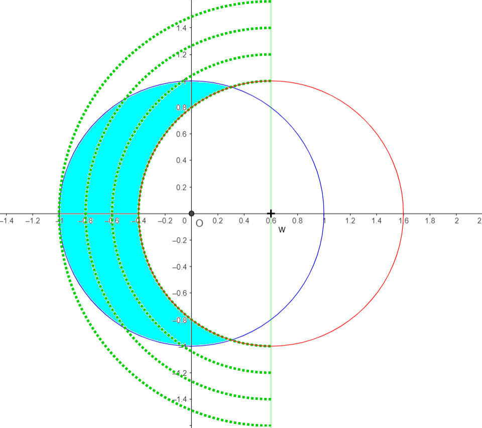
Figure 1. Figure of the situation for $d=2$ and $r=0.6$.
The left hand side set of (35) is in blue, the sets $S^{1/2}(\omega,1+t)$ for $t\in\{0;0.2;0.4;0.6\}$ are shown in green

3.2.3. Rest of the proof

Rest of the proof works almost word by word.

Appendix A Proof of Proposition 2.3

In this subsection we will prove Proposition 2.3 by following a strategy similar to the one in [Wal86].

As in [Wal86, p. 343], using (4) we obtain that the solution $u_{\_}t$ of the SHE as defined in (3) can be written, for every $f\in C^{\infty}(\mathbb{R}^{d})$,

$$u_{\_}t(f)=\sum_{\_}{n=0}^{\infty}\langle f\leavevmode\nobreak\ |\leavevmode\nobreak\ f_{\_}n\rangle\int_{\_}0^{t}\int_{\_}Da(y)e^{-\mu_{\_}n(t-s)}f_{\_}n(y)W(dy,ds).$$

Thus, noting $A_{\_}n(t):=\int_{\_}0^{t}\int_{\_}Da(y)e^{-\mu_{\_}n(t-s)}f_{\_}n(y)W(dy,ds)$, this justificates the notation with the infinite sum

$$u_{\_}t:=\sum_{\_}{n=0}^{\infty}A_{\_}n(t)f_{\_}n.$$

We will now prove that the random variables $A_{\_}n(t)$ are solutions to the Itô SDEs (5), and that the $B_{\_}t^{n}$ are brownian motions of covariation given by $\text{Cor}(B_{\_}t^{n},B_{\_}s^{m})=t\langle af_{\_}n\leavevmode\nobreak\ |\leavevmode\nobreak\ af_{\_}m\rangle$.
 
Noting $B_{\_}t^{n}:=\int_{\_}0^{t}\int_{\_}Da(y)f_{\_}n(y)W(dy,ds)$, we can immediatly see with Itô’s formula that the $A_{\_}n(t)$ checks (5). Moreover, a common property of Walsh’s integral is that each $B_{\_}t^{n}$ are martingales whose quadratic covariation is given by

$$\text{Cor}(B_{\_}t^{n},B_{\_}s^{m})=\int_{\_}0^{t}\int_{\_}Da(x)f_{\_}n(x)a(x)f_{\_}m(x)dx\,ds=t\langle af_{\_}n\leavevmode\nobreak\ |\leavevmode\nobreak\ af_{\_}m\rangle.$$

To conclude, one should still prove that this characterizes uniquely $u_{\_}t$. To do so, since the Ornstein-Uhlenbeck SDEs (5) admit a unique weak solution, it is enough to prove that the joint law of the process $(B_{\_}t^{n}\leavevmode\nobreak\ :\leavevmode\nobreak\ t\geq 0)_{\_}{n\geq 0}$ is uniquely determined by the condition $\text{Cor}(B_{\_}t^{n},B_{\_}t^{m})=t\langle af_{\_}n\leavevmode\nobreak\ |\leavevmode\nobreak\ af_{\_}m\rangle$.
We choose $k\geq 1$, a finite subset $(n_{\_}1,\dots,n_{\_}k)\subset\mathbb{N}$ and $c=(c_{\_}1,\dots,c_{\_}k)\in\mathbb{R}^{k}$. We pose $m_{\_}t:=\sum_{\_}{i=1}^{k}c_{\_}iB_{\_}t^{n_{\_}i}$ a martingale such that, noting $\langle\cdot\leavevmode\nobreak\ |\leavevmode\nobreak\ \cdot\rangle_{\_}t$ the quadratic variation,

$$\langle m\rangle_{\_}t=\sum_{\_}{i,j=1}^{k}c_{\_}ic_{\_}j\langle B^{n_{\_}i}\leavevmode\nobreak\ |\leavevmode\nobreak\ B^{n_{\_}j}\rangle_{\_}t=t\sum_{\_}{i,j=1}^{k}c_{\_}ic_{\_}j\langle af_{\_}{n_{\_}i}\leavevmode\nobreak\ |\leavevmode\nobreak\ af_{\_}{n_{\_}j}\rangle=t(c^{\dagger}\cdot A\cdot c),$$

where $A:=(\langle af_{\_}{n_{\_}i}\leavevmode\nobreak\ |\leavevmode\nobreak\ af_{\_}{n_{\_}j}\rangle)_{\_}{1\leq i,j\leq k}$ and $v^{\dagger}$ is the transposed vector of a vector $v\in\mathbb{R}^{d}$. Thus the exponential martingale associated to $m_{\_}t$ is

$$\mathcal{E}(im)_{\_}t=\exp\left(im_{\_}t+\frac{t}{2}(c^{\dagger}\cdot A\cdot c)\right),$$

and is also a martingale. Thus, for $0\leq s\leq t$,

$$\mathbb{E}\left[\exp\left(ic^{\dagger}\cdot(m_{\_}t-m_{\_}s)\right)\leavevmode\nobreak\ |\leavevmode\nobreak\ \mathcal{F}_{\_}s\right]=\exp\left(-\dfrac{t-s}{2}(c^{\dagger}\cdot A\cdot c)\right).$$

We recognize the characteristic function of a multidimensional normal distribution such that the law of $m_{\_}t-m_{\_}s$ conditionnaly to $\mathcal{F}_{\_}s$ is $\mathcal{N}(0,(t-s)A)$. Thus, $m_{\_}t$ follows the law of a continuous Lévy process of $\mathcal{N}(0,(t-s)A)$ increments. This characterizes uniquely the law of $m_{\_}t$, and furthermore the law of the process $(B_{\_}t^{n}\leavevmode\nobreak\ :\leavevmode\nobreak\ t\geq 0)_{\_}{n\geq 0}$.

Appendix B Lemma for identifying martingales

Lemma B.1.

Let $(\Omega,\mathcal{F},(\mathcal{F}_{\_}t)_{\_}{t\geq 0},\mathbb{P})$ be a filtred probability space.
If $(X_{\_}t)_{\_}t$ is a $\mathcal{F}_{\_}t$-adapted process taking values in a Banach space $(B,|\cdot|)$ such that there exist $\mathcal{F}_{\_}t$-adapted processes $(A_{\_}t)_{\_}{t\geq 0}$ and $(o_{\_}s(t))_{\_}{s,t\geq 0}$ verifying for every $h:=t-s$,

$$\mathbb{E}[X_{\_}t\leavevmode\nobreak\ |\leavevmode\nobreak\ \mathcal{F}_{\_}s]=X_{\_}s+hA_{\_}s+o_{\_}s(h),$$

where

• the random variables $o_{\_}s$ check $\mathbb{E}|o_{\_}s(h)|\leq Co(h)$, where $C$ is a constant,

• the fonction $t\mapsto A_{\_}t$ is almost surely cadlag and Bochner-integrable,

• for all $T>0$, we have $\mathbb{E}\sup_{\_}{t\leq T}|A_{\_}t|<\infty$.

Then the process

$$Y_{\_}t:=X_{\_}t-\int_{\_}0^{t}A_{\_}sds,$$

is a $\mathcal{F}_{\_}t$-martingale.

Proof.

Let $t>s\geq 0$, and prove that

(36) $$\mathbb{E}\left|\leavevmode\nobreak\ \mathbb{E}\left[X_{\_}t-X_{\_}s-\int_{\_}s^{t}A_{\_}rdr\leavevmode\nobreak\ \Big{|}\leavevmode\nobreak\ \mathcal{F}_{\_}s\right]\leavevmode\nobreak\ \right|=0.$$

We compute, with $\cup_{\_}{i=1}^{n}[s_{\_}i,t_{\_}i)$ an uniform partition of $[s,t)$ (ie such that $t_{\_}i-s_{\_}i=h$ and $nh=t-s$)

$$\mathbb{E}\left|\leavevmode\nobreak\ \mathbb{E}\left[X_{\_}t-X_{\_}s-\int_{\_}s^{t}A_{\_}r+dr\leavevmode\nobreak\ \Big{|}\leavevmode\nobreak\ \mathcal{F}_{\_}s\right]\leavevmode\nobreak\ \right| =\mathbb{E}\left|\leavevmode\nobreak\ \mathbb{E}\left[\sum_{\_}{i=1}^{n}X_{\_}{t_{\_}i}-X_{\_}{s_{\_}i}-\int_{\_}s^{t}A_{\_}rdr\leavevmode\nobreak\ \Big{|}\leavevmode\nobreak\ \mathcal{F}_{\_}s\right]\leavevmode\nobreak\ \right|$$

$$=\mathbb{E}\left|\leavevmode\nobreak\ \mathbb{E}\left[\sum_{\_}{i=1}^{n}hA_{\_}{s_{\_}i}+o_{\_}{s_{\_}i}(h)-\int_{\_}s^{t}A_{\_}rdr\leavevmode\nobreak\ \Big{|}\leavevmode\nobreak\ \mathcal{F}_{\_}s\right]\leavevmode\nobreak\ \right|$$

$$\leq\mathbb{E}\left|\sum_{\_}{i=1}^{n}hA_{\_}{s_{\_}i}-\int_{\_}s^{t}A_{\_}rdr\right|+\sum_{\_}{i=1}^{n}\mathbb{E}|o_{\_}{s_{\_}i}(h)|$$

By the assumption (i), we have that $\sum_{\_}{i=1}^{n}\mathbb{E}|o_{\_}{s_{\_}i}(h)|\mapsto 0$ for $n\mapsto\infty$.
By the assumption (ii) we have that $\sum_{\_}{i=1}^{n}hA_{\_}{s_{\_}i}\mapsto\int_{\_}s^{t}A_{\_}rdr$ almost surely for $n\mapsto\infty$, and with assumption (iii) we can use the Bochner dominated convergence theorem to prove that the convergence is also in $L^{1}(\Omega)$.
Thus, (36) indeed holds and $Y_{\_}t$ is a $\mathcal{F}_{\_}t$-martingale. ∎

Appendix C Lemma 2.8

Proof of Lemma 2.8.

From Lemma 2.6

$$\mathbb{E}\left[\varphi_{\_}D^{B(x,\varepsilon^{\prime})}(x)^{4}\right] =\mathbb{E}\left[\varphi_{\_}D^{B(x,\varepsilon)}(x)^{4}\right]+\mathbb{E}\left[\left((\tilde{h}^{B(x,\varepsilon)},\eta_{\_}x^{\varepsilon^{\prime}})-(\tilde{h}^{B(x,\varepsilon^{\prime})},\eta_{\_}x^{\varepsilon^{\prime}})\right)^{4}\right]$$

$$+6\mathbb{E}\left[\varphi_{\_}D^{B(x,\varepsilon)}(x)^{2}\left((\tilde{h}^{B(x,\varepsilon)},\eta_{\_}x^{\varepsilon^{\prime}})-(\tilde{h}^{B(x,\varepsilon^{\prime})},\eta_{\_}x^{\varepsilon^{\prime}})\right)^{2}\right].$$

and the first point follows. Now, define $2^{-n}\leq\varepsilon<2^{-(n-1)}$ and $n_{\_}0:=\inf\{m\leq n\leavevmode\nobreak\ :\leavevmode\nobreak\ 2^{-m}<\delta\}$. Then $\mathbb{E}\left[\varphi_{\_}D^{B(x,\varepsilon)}(x)^{2}\right]\leq\mathbb{E}\left[\varphi_{\_}D^{B(x,2^{-n})}(x)^{2}\right]$. Using the above identity several times we obtain

$$\mathbb{E}\left[\varphi_{\_}D^{B(x,2^{-n})}(x)^{4}\right]=\mathbb{E}\left[\varphi_{\_}D^{B(x,2^{-n_{\_}0})}(x)^{4}\right]+\sum_{\_}{m=n_{\_}0}^{n-1}\mathbb{E}\left[\varphi_{\_}{B(x,2^{-m})}^{B(x,2^{-(m+1)})}(x)^{4}\right]$$

$$+\sum_{\_}{m=n_{\_}0}^{n-1}\mathbb{E}\left[\varphi_{\_}D^{B(x,2^{-n_{\_}0})}(x)^{2}\varphi_{\_}{B(x,2^{-m})}^{B(x,2^{-(m+1)})}(x)^{2}\right]+2\sum_{\_}{m>m^{\prime}=n_{\_}0}^{n-1}\mathbb{E}\left[\varphi_{\_}{B(x,2^{-m})}^{B(x,2^{-(m+1)})}(x)^{2}\varphi_{\_}{B(x,2^{-m^{\prime}})}^{B(x,2^{-(m^{\prime}+1)})}(x)^{2}\right].$$

We can bound this by

$$\mathbb{E}\left[(h^{D},\eta_{\_}x^{2^{-n_{\_}0}})^{4}\right]+\sum_{\_}{m=n_{\_}0+1}^{n-1}\mathbb{E}\left[(\tilde{h}^{B(x,2^{-(m-1)})},\eta_{\_}x^{2^{-m}})^{4}\right]+\mathbb{E}\left[(h^{D},\eta_{\_}x^{2^{-n_{\_}0}})^{2}\right]\sum_{\_}{m=n_{\_}0+1}^{n-1}\mathbb{E}\left[(\tilde{h}^{B(x,2^{-(m-1)})},\eta_{\_}x^{2^{-m}})^{4}\right].$$

The uniform bound on the 4th moments (point B in the definition) bounds the first term by a constant that depends on $\delta$. Further $\sup_{\_}{x\in D}\eta_{\_}x^{2^{-m}}\leq 2^{md}$ and thus the MTD condition bounds each of the other terms by $2^{4md}2^{-(m-1)2(d+2)}=2^{2(d+2)}2^{2m(d-2)}$. Finally the third term can be handled as in the proof of Lemma 2.7 with a constant depending on $\delta$. Summing now together, we obtain the relevant bounds.
Using Hölder’s inequality, one can deduce the last identity.∎

Appendix D The analogue of Lemma 2.7 in the fractional case

Proof.

From the analog of Lemma 2.6 and Assumption A’ we can write

$$\mathbb{E}\left[\varphi_{\_}D^{B(x,\varepsilon^{\prime})}(x)^{2}\right]=\mathbb{E}\left[\varphi_{\_}D^{B(x,\varepsilon)}(x)^{2}\right]+\mathbb{E}\left[\left((\tilde{h}^{B(x,\varepsilon)},A_{\_}x^{\varepsilon^{\prime}})-(\tilde{h}^{B(x,\varepsilon^{\prime})},A_{\_}x^{\varepsilon^{\prime}})\right)^{2}\right]$$

and the first point follows.
Now, define $2^{-n}\leq\varepsilon<2^{-(n-1)}$ and $n_{\_}0:=\inf\{m\leq n\leavevmode\nobreak\ :\leavevmode\nobreak\ 2^{-m}<\delta\}$. Then $\mathbb{E}\left[\varphi_{\_}D^{B(x,\varepsilon)}(x)^{2}\right]\leq\mathbb{E}\left[\varphi_{\_}D^{B(x,2^{-n})}(x)^{2}\right]$. Using the above identity several times we obtain

$$\mathbb{E}\left[\varphi_{\_}D^{B(x,2^{-n})}(x)^{2}\right]=\mathbb{E}\left[\varphi_{\_}D^{B(x,2^{-n_{\_}0})}(x)^{2}\right]+\sum_{\_}{m=n_{\_}0+1}^{n-1}\mathbb{E}\left[\left((\tilde{h}^{B(x,2^{-(m-1)})},A_{\_}x^{2^{-m}})-(\tilde{h}^{B(x,2^{-m})},A_{\_}x^{2^{-m}})\right)^{2}\right].$$

We can bound this by

$$\mathbb{E}\left[(h^{D},A_{\_}x^{2^{-n_{\_}0}})^{2}\right]+\sum_{\_}{m=n_{\_}0+1}^{n-1}\mathbb{E}\left[(\tilde{h}^{B(x,2^{-(m-1)})},A_{\_}x^{2^{-m}})^{2}\right].$$

With FMTD’s second moment and (27), we have $\mathbb{E}\left[(\tilde{h}^{B(0,2\varepsilon)},A_{\_}x^{\varepsilon})^{2}\right]=\varepsilon^{2\alpha+d}\mathbb{E}\left[(h^{D},A_{\_}x^{\varepsilon}(2\varepsilon\cdot))^{2}\right]=\varepsilon^{2\alpha-d}\mathbb{E}\left[(h^{D},A_{\_}x^{1/2})^{2}\right]$, such that we get

$$\mathbb{E}\left[\varphi_{\_}D^{B(x,\varepsilon)}(x)^{2}\right]\leq C\left(1+\sum_{\_}{m=n_{\_}0+1}^{n-1}2^{m(d-2\alpha)}\right),$$

where the constant $C>0$ depends on $C_{\_}a$ and $n_{\_}0$ and thus on $\delta$. Computing the sum, we obtain

$$\mathbb{E}\left[\varphi_{\_}D^{B(x,\varepsilon)}(x)^{2}\right]\leq C(\delta)\left(1+\varepsilon^{2\alpha-d}\right).$$

∎

References

• [ABR01] S. Axler, P. Bourdon, and W. Ramey. Harmonic Function Theory. Graduate Texts in Mathematics. Springer, 2001.
• [AP22] Juhan Aru and Ellen Powell. A characterisation of the continuum gaussian free field in arbitrary dimensions. Journal de l’École polytechnique—Mathématiques, 9:1101–1120, 2022.
• [BBK+09] Krzysztof Bogdan, Tomasz Byczkowski, Tadeusz Kulczycki, Michal Ryznar, Renming Song, and Zoran Vondracek. Potential analysis of stable processes and its extensions. Springer Science & Business Media, 2009.
• [BDV20] Claudia Bucur, Serena Dipierro, and Enrico Valdinoci. On the mean value property of fractional harmonic functions. Nonlinear Analysis, 201:112112, 2020. Nonlinear Analysis and Partial Differential Equations Special Issue in honor of Professor Shair Ahmad on the occasion of his 85th birthday and his retirement.
• [BLR20] N. Berestycki, B. Laslier, and G. Ray. Dimers and imaginary geometry. Ann. Probab., 48(1):1–52, 2020.
• [BPR20] N. Berestycki, E. Powell, and G. Ray. A characterisation of the Gaussian free field. Probab. Theory Related Fields, 176(3):1259–1301, 2020.
• [BPR21] N. Berestycki, E. Powell, and G. Ray. $(1+\varepsilon)$-moments suffice to characterise the Gaussian free field. Electronic Journal of Probability, 2021.
• [Buc16] Claudia Bucur. Some observations on the green function for the ball in the fractional laplace framework, 2016.
• [CS98] Zhen-Qing Chen and Renming Song. Estimates on green functions and poisson kernels for symmetric stable processes. Mathematische Annalen, 312:465–501, 1998.
• [CS24] Sky Cao and Scott Sheffield. Fractional gaussian forms and gauge theory: an overview, 2024.
• [EK09] Stewart N Ethier and Thomas G Kurtz. Markov processes: characterization and convergence. John Wiley & Sons, 2009.
• [FKN11] Mohammud Foondun, Davar Khoshnevisan, and Eulalia Nualart. A local-time correspondence for stochastic partial differential equations. Transactions of the American Mathematical Society, 363(5):2481–2515, 2011.
• [Gar24] Christophe Garban. Invisibility of the integers for the discrete gaussian chain via a caffarelli-silvestre extension of the discrete fractional laplacian, 2024.
• [GP24] Trishen S. Gunaratnam and Romain Panis. Emergence of fractional gaussian free field correlations in subcritical long-range ising models, 2024.
• [HNS09] Yaozhong Hu, David Nualart, and Jian Song. Fractional martingales and characterization of the fractional brownian motion. 2009.
• [Ken01] R. Kenyon. Dominos and the Gaussian free field. Ann. Probab., 29(3):1128–1137, 2001.
• [LPG+20] Anna Lischke, Guofei Pang, Mamikon Gulian, Fangying Song, Christian Glusa, Xiaoning Zheng, Zhiping Mao, Wei Cai, Mark M. Meerschaert, Mark Ainsworth, and George Em Karniadakis. What is the fractional laplacian? a comparative review with new results. Journal of Computational Physics, 404:109009, 2020.
• [LS20] SV Lototsky and Apoorva Shah. Gaussian fields and stochastic heat equations. 2020.
• [LSSW14] Asad Lodhia, Scott Sheffield, Xin Sun, and Samuel Watson. Fractional gaussian fields: A survey. Probability Surveys, 13, 07 2014.
• [Mit83] Itaru Mitoma. Tightness of probabilities on c ([0, 1]; y’) and d ([0, 1]; y’). The Annals of Probability, pages 989–999, 1983.
• [MV11] Yuliya Mishura and Esko Valkeila. An extension of the lévy characterization to fractional brownian motion. 2011.
• [Nad97] T. Naddaf, A.and Spencer. On homogenization and scaling limit of some gradient perturbations of a massless free field. Comm. Math. Phys., 183(1):55–84, 1997.
• [RV07] B. Rider and B. Virág. The noise in the circular law and the Gaussian free field. Int. Math. Res. Not. IMRN, 2, 2007.
• [Wal86] J. B. Walsh. An introduction to Stochastic Partial Differential Equations. Ecole d’été de probabilités de Saint-Flour, 1986.