Computational quantum transport

Abstract

This review is devoted to the different techniques that have been developed to compute the coherent transport properties of quantum nanoelectronic systems connected to electrodes. Beside a review of the different algorithms proposed in the literature, we provide a comprehensive and pedagogical derivation of the two formalisms on which these techniques are based: the scattering approach and the Green’s function approach. We show that the scattering problem can be formulated as a system of linear equations and that different existing algorithms for solving this scattering problem amount to different sequences of Gaussian elimination. We explicitly prove the equivalence of the two formalisms. We discuss the stability and numerical complexity of the existing methods.

I Introduction

The field of quantum nanoelectronics, also as “mesoscopic physics” was born in the early eighties with the first experiments directly illustrating the impact of the wave nature of electrons on macroscopic observables such as the electrical conductance. While already before it was known that quantum mechanics plays a role in the transport properties, this role was restricted to the material band structure, i.e., to its behavior on atomic scale, while the physics at larger scales was described by a semi-classical incoherent theory—Boltzmann equation. Such a description was adequate until it became possible to study the transport properties of samples at ultra-low temperatures or to make very small devices. At low temperature, the characteristic length $L_{\Phi}$ over which the electron wave function retains a well-defined phase becomes large and eventually exceeds the device size. The demonstration of the quantum Hall effect [136] and the phenomena of universal conductance fluctuations or the weak localization [6] were early observations of the impact of the wave nature of electrons in electronic devices made indirectly in bulk samples. Later, as clean room technology made possible to pattern increasingly smaller devices, direct observation of, e.g., the Aharonov-Bohm effect in a small metal loop [300] or the conductance quantization in a constriction [302] became possible. Nowadays, the phase coherence length has reached record, almost macroscopic, values $L_{\Phi}\approx$250\text{\,}\mathrm{\SIUnitSymbolMicro m}$$ making possible to envision operating these interferometers to make flying quantum bits or other complex manipulations of quantum states [48].

Building a theoretical understanding of the quantum transport phenomena required figuring out how one connects the macroscopic world, where one injects currents and measures voltage differences, to the mesoscopic scale described by quantum mechanics. Landauer proposed that the problem could be formulated as a waveguide problem where the electrodes are treated as infinite waveguides with well-defined incoming waves. This viewpoint eventually lead to a number of striking predictions including the conductance quantization and the separation between the cause of finite electrical resistance (elastic scattering) and the corresponding Joules heating that takes place in the electrodes. The theory eventually evolved into two very different looking, albeit strictly equivalent, approaches to quantum transport. In the Landauer-Büttiker or scattering formalism, one treats the quantum-mechanical system as a scattering problem and arrives at the celebrated Landauer formula. The other approach relies on the Keldysh perturbation theory to build the non-equilibrium Green’s functions (NEGF) formalism.

Computational quantum transport, that aims to calculate the transport properties of coherent samples numerically, is almost as old as mesoscopic physics itself. Interference effects are indeed very sensitive to microscopic details so that, as P. W. Anderson stated in his 1977 Nobel lecture, in the context of localization, “one has to resort to the indignity of numerical simulations to settle even the simplest questions about it”. Despite their indignity, numerical simulations of quantum transport have become increasingly popular and powerful. This work aims to provide a systematic review of the techniques that were developed to perform such computations.

I.1 Scope of this review

This review focuses on computational techniques that address coherent quantum transport for discrete models that consist of a finite system connected to semi-infinite quasi-one-dimensional electrodes. We omit the calculation of local quantities (e.g., conductivities) already described in other reviews [304, 83]. These calculations are based on linear response Kubo formula [146, 102] which may or may not capture non-local effects depending on the level of approximation [26]. Here, we focus on techniques that focus on global quantities (e.g., conductances).

The goals of this article are threefold:

1. provide a detailed pedagogical entry point for newcomers to the field,

2. present a modern and comprehensive derivation of the mathematical formalism for both the scattering approach and NEGF as well as the equivalence between the two,

3. review the relevant literature with a stress on the algorithms, as well as a few selected applications.

The techniques introduced in this review have a broad range of applications, including devices combining multiple materials semiconductors, superconductors, magnetic materials, metals, graphene, topological insulators in a wide variety of geometries and in different dimensions. Due to the vastness of the applications, it is not feasible for us to review all of them in detail. Instead we will cover several illustrative examples that demonstrate the benefits provided by computational quantum transport in analyzing physical phenomena.

Although most of the material presented in this review is known, some aspects were not presented before at this level of generality and/or within a unified formalism. We also include some new material: specifically the detailed algorithms that were developed for the Kwant package [104] that were not yet published.

I.2 A short history of computational quantum transport

The scattering approach to quantum transport was initially defined in [153] and further extended by [87, 49, 271]. The approach is reviewed in [35] or [71]. The first formulations of the scattering problem for discrete models can be traced down to [159] in the nanoelectronics community and [15] in the physics community. The alternative NEGF theory is based on the Keldysh formalism [133] which considerably simplifies in the context of non-interacting systems [55]. The point of reference in the field is the work [191], which generalizes [55] to interacting systems.

The first numerical calculation of the electrical conductance of a quantum system was made in [278] and [158] where the recursive Green’s function (RGF) algorithm was introduced for a one-dimensional system. The RGF was soon to become the reference of the field thanks to several groups that generalized it to quasi-one-dimensional systems [181] and developed the equivalent wave function approach [15]. The initial applications of RGF focused on tight-binding systems with a square lattice and a rectangular geometry for studying Anderson localization, quantum dots, quantum billiards, or other mesoscopic systems. This early code was considered highly useful, to the extent that its reference implementation was referred to as “the Program” in some research groups.

These numerical techniques were then generalized to tackle a wider class of problems including general lattices (most prominently the graphene honeycomb structure), multi-terminal systems, systems with internal degrees of freedom (e. g. spin or electron/hole for superconductivity), and arbitrary geometries beyond the rectangular shape that was natural in RGF [130, 307], and extensions beyond quasi one-dimensional systems [256]. Various strategies to accelerate the calculations were also developed, including algorithms that precalculate building blocks [241, 276], parallel algorithms [78, 147, 63], slicing strategies for recursive algorithms [307, 197, 189, 277], or nested dissection [165, 40]. The range of applications expanded considerably to a much wider spectrum including mesoscopic superconductivity, electronic interferometers, quantum Hall effect, spintronics, graphene, any combination of the above and much more.

While most codes remain internal to the research groups where they have been developed, publicly available and open source codes have started to be developed. These include SMEAGOL [238], nextnano [33], Knit [130], Kwant [104], and Quantica.jl [249]. There exist also quantum transport extensions to ab-initio packages such as TransSIESTA [42], OpenMX [209], NanoTCAD Vides [18, 44], GOLLUM [85], and Nemo5 [117].

I.3 How to read this review

This review first establishes the scattering matrix formalism, and uses it to derive the NEGF formalism. Attention has been taken to derive both formalisms using unified notation and to gather a comprehensive set of proofs, including several original ones.

In order to not overwhelm the readers with the technical details, we start with a pedagogical Sec. II that introduces the main concepts: scattering wave functions, scattering matrix, and Landauer formula using the minimal example of a square lattice, which allows to keep the notation and the derivation simple. Readers not familiar with the scattering theory can use this section as an entry point to the field, but experts can skip this section altogether.

Sec. III introduces the scattering problem as a set of linear equations whose solution defines both the scattering wave function and the scattering matrix. It also introduces the notation used in the rest of the review. Solving for both the wave function and the scattering matrix at the same time is not entirely standard in the field, we name it the $\Psi S$-approach. It forms the backbone of this review from which all the other approaches are derived. This section maintains maximal generality, only assuming discrete models and translationally invariant leads. Sec. IV expands on Sec. III by transforming the scattering problem into a form that is stable for numerical calculations.

We establish the relation to NEGF in Sec. V by introducing the retarded Green’s function using a linear problem approach, similar to the one that defines the scattering formalism. While this is an uncommon approach, it has the advantage of emphasizing the close analogy between the scattering matrix and the Green’s function techniques and allowing for a direct derivation of the Fisher–Lee relations that connect one with the other. Sec. V ends with making contact with the more standard approach to Green’s function that uses the Dyson equation and the RGF class of algorithms.

Sections III, IV and V only deal with the single particle quantum mechanics of infinite systems (or more precisely finite systems connected to semi-infinite electrodes) as well as the algorithms used to solve the corresponding mathematical problems. In order to calculate observables, such as the electrical conductance, quantum mechanics must be complemented with out-of-equilibrium statistical physics. Sec. VII introduces various observables that can be obtained from the scattering matrix ranging from the conductance (Landauer formula) to current noise and thermoelectric effects. Sec. VIII describes the NEGF approach for the calculations of the observables. Although the two approaches look very different, we establish their complete equivalence. Sections VII and VIII end the technical part of this review.

We end this review with a brief overview of different models used in computational quantum transport and a selection of prominent applications. It is impossible for this part of the review to be exhaustive, and we restrict ourselves to a few examples that illustrate the main theoretical concepts. We somewhat artificially split the discussion of the applications in two sections: the top-down and bottom-up approaches to modeling. Sec. IX discusses applications that make use of the model Hamiltonians originating in the effective minimal models of physical materials. We demonstrate how these models apply to a wide range of systems and phenomena: mesoscopic superconductivity, spintronics, topological materials, and graphene. In contrast, Sec. X introduces the Hamiltonian models from ab-initio or atomistic calculations. These models are more realistic and precise, but also more limited in their range of applicability.

II A pedagogical example: conductance of samples cut out of a two-dimensional electron gas

We begin by demonstrating in a pedagogical manner how different concepts of computational quantum transport apply to a minimal example. Readers who are already experienced with the concepts of scattering matrix, self-energy, or the Landauer formula for the conductance can skip this part altogether. Because a number of sources already describes in detail the non-computational aspects of the scattering formalism of quantum transport (see, e.g., [71]), we restrict ourselves to a concise presentation of the basic concepts.

We consider a fully coherent quantum conductor connected to two perfect electrodes—leads—where all the dissipation takes place. This is an idealized situation: in a real device, electrons always experience some dephasing due to, e.g., coupling to phonons or electron-electron interaction. Nevertheless, typical dephasing lengths at dilution fridge temperature ($\sim$10\text{\,}\mathrm{mK}$$) can exceed tens of microns, and as device sizes continue to shrink, this model captures the salient features of many realistic devices.

II.1 The Schrödinger equation as a waveguide problem

Figure 1: Sketch of a quasi one-dimensional wire of width $\mathcal{W}$. The shaded scattering region in the middle symbolizes an arbitrary potential that scatters the plane waves coming from the left into reflected ($r$) and transmitted ($t$) wave.

We consider the quantum mechanics of an electron confined in the simple geometry sketched in Fig. 1: a two-dimensional wire that is infinite in the $x$ direction, has width $\mathcal{W}$ in $y$-direction, and contains a scattering region of size $\mathcal{L}$. Our first task is to solve the spinless Schrödinger equation for the problem:

$$\frac{\hbar^{2}}{2m^{*}}\Delta\Psi(x,y)+V(x,y)\Psi(x,y)=E\Psi(x,y),$$ (1)

where $m^{*}$ is the electronic effective mass, $E$ is the energy of the electron, $\Psi$ is its wave function, and $V(x,y)$ is an arbitrary potential, which is non-zero in a finite region $0<x<\mathcal{L}$ of the wire. The boundary conditions require that $\Psi$ vanishes at the wire boundaries: $\Psi(x,y=0)=\Psi(x,y=\mathcal{W})=0$. To construct the full solutions of this equation, we first analyze it outside of the scattering region, where $V(x,y)=0$, and the system is therefore translationally invariant. In that case the solutions are linear superpositions of plane waves $\exp(ik_{x}x+ik_{y}y)$ with $E=\hbar^{2}/(2m^{*})(k_{x}^{2}+k_{y}^{2})$. Imposing the boundary conditions at $y=0$ and $y=\mathcal{W}$ further restricts the wave functions to be linear combinations of $e^{ik_{x}x}\sin(k_{y}y)$, with $k_{y}=\alpha\pi/\mathcal{W}$, where $\alpha$ is an integer that labels lead modes. The dispersion relation requires that $k_{x}=\pm k_{\alpha}\equiv\pm\sqrt{2m^{*}E/\hbar^{2}-(\pi\alpha/\mathcal{W})^{2}}$. For the $N_{p}$ values of $\alpha$ such that $\hbar^{2}k_{y}^{2}/2m^{*}<E$, $k_{\alpha}$ is real and positive. These modes are, therefore, propagating: they extend to $x\to\pm\infty$, and they define conduction channels. Infinitely many modes with $\alpha>N_{p}$ have imaginary $k_{\alpha}$, and are exponentially decaying either to the left or to the right from the scattering region. We therefore parametrize the wave function left of the scattering region ($x<0$) using

$$\Psi(x,y)=\sum_{\alpha}\frac{\sin\left(\pi\alpha y/\mathcal{W}\right)}{\sqrt{\mathcal{W}|k_{\alpha}|/2}}\left[q_{L-,\alpha}e^{ik_{\alpha}x}+q_{L+,\alpha}e^{-ik_{\alpha}x}\right],$$ (2a)

and accordingly on the right of the scattering region ($$x>\mathcal{L}$$) using

$$\Psi(x,y)=\sum_{\alpha}\frac{\sin\left(\pi\alpha y/\mathcal{W}\right)}{\sqrt{\mathcal{W}|k_{\alpha}|/2}}\left[q_{R+,\alpha}e^{ik_{\alpha}x}+q_{R-,\alpha}e^{-ik_{\alpha}x}\right].$$ (2b)

This asymptotic wave function is parametrized using coefficients $q_{L/R,\pm,\alpha}$, which are yet undetermined. The $L/R$ subscript labels the left and right sides of the scattering region, while $+$ and $-$ label the modes propagating towards or away from the scattering region, regardless of the side. While the normalization constants $(W|k_{\alpha}|/2)^{-1/2}$ may be absorbed in the definition of $q_{L/R,\pm,\alpha}$, we introduce them for later convenience. Determining the values of the $q_{L/R,\pm,\alpha}$ requires solving the Schrödinger equation in the difficult scattering region, and then matching the wave function in the different parts of the system by using the continuity of the wave function and its derivative. Furthermore, for the wave function to not diverge away from the scattering region, the solutions that diverge at $x\to\pm\infty$ must be absent: $q_{L-,\alpha}=q_{R-,\alpha}=0$ for $\alpha>N_{p}$. Unless $V(x,y)$ belongs to a narrow class of sufficiently simple potentials, the wave function matching admits no analytical solution and must be obtained numerically (hence this review!). Despite that, we can draw several predictions about the general properties of the solution without having it.

II.2 The scattering matrix

The wave matching problem is underdetermined, and therefore admits infinitely many solutions. We, therefore describe its solutions by expressing some unknown parameters $q_{L/R,\pm,\alpha}$ through the others. Setting one of the $q_{L/R,-,\alpha_{0}}$ to be unity and all other $q_{L/R,-,\alpha_{0}}$ to zero, for $\alpha_{0}<N_{p}$ allows to determine a unique value of all the other coefficients. Collecting these solutions into a matrix allows to relate the amplitudes of the propagating modes using the scattering matrix $S$:

$$\begin{pmatrix}q_{L+}\\ q_{R+}\end{pmatrix}=S\begin{pmatrix}q_{L-}\\ q_{R-}\end{pmatrix}\equiv\begin{pmatrix}r&t^{\prime}\\ t&r^{\prime}\end{pmatrix}\begin{pmatrix}q_{L-}\\ q_{R-}\end{pmatrix},$$ (3)

where $q_{L/R\pm}$ are size $N_{p}$ vector containing all the coefficients of the propagating modes. The different blocks of the $S$-matrix are the reflection ($r,r^{\prime}$) and transmission ($t,t^{\prime}$) matrices.

Let us check how current conservation applies to the $S$-matrix. The total particle current $I_{p}$ flowing through the wire,

$$I_{p}=\frac{\hbar}{m^{*}}\int_{0}^{\mathcal{W}}dy\operatorname{Im}\Psi^{*}(x,y)\partial_{x}\Psi(x,y),$$ (4)

is independent of $x$ for any solution of Eq. (1). Substituting Eq. (2) into Eq. (4) yields

$$\sum_{\alpha=1}^{N_{p}}|q_{L+,\alpha}|^{2}+|q_{R+,\alpha}|^{2}=\sum_{\alpha=1}^{N_{p}}|q_{L-,\alpha}|^{2}+|q_{R-,\alpha}|^{2},$$ (5)

where we have used the orthogonality of the transverse wave function $\int_{0}^{\mathcal{W}}dy\sin(\pi\alpha y/\mathcal{W})\sin(\pi\beta y/\mathcal{W})=\delta_{\alpha\beta}(\mathcal{W}/2)$. We also see that the normalization constants in Eqs. (2) are chosen so that the Eq. (5) has no prefactors. For every solution (3) of the scattering problem to satisfy Eq. (5), the $S$-matrix must preserve norm of vectors, or in other words it must be unitary:

$$SS^{\dagger}=S^{\dagger}S=1.$$ (6)

Similarly to how the Hermiticity of the Hamiltonian leads to current conservation and the unitarity of $S$, other properties of the Hamiltonian give other constraints to $S$. For example, in presence of a magnetic field $B$ with a vector potential $\vec{A}(x,y)$, the Hamiltonian becomes

$$H=\frac{1}{2m^{*}}\left(i\hbar\vec{\nabla}-e\vec{A}\right)^{2}+V(x,y).$$ (7)

One observes that if $\Psi(x,y)$ is an eigenstate of Eq. (7) with magnetic field $B$ and vector potential $\vec{A}$, then $\Psi(x,y)^{*}$ is an eigenstate at the same energy, field $-B$, and vector potential $-\vec{A}$. While the mode wave functions in Eqs. (2) are not Hamiltonian eigenstates in presence of a vector potential, a similar decomposition into lead modes still holds. Taking the complex conjugate of Eqs. (2) conjugates the amplitudes $q_{L/R\pm,\alpha}$ and exchanges the outgoing ($+$) and incoming ($-$) propagating modes. The Eq. (3) then transforms into

$$\begin{pmatrix}q_{L-}^{*}\\ q_{R-}^{*}\end{pmatrix}=S(-B)\begin{pmatrix}q_{L+}^{*}\\ q_{R+}^{*}\end{pmatrix}.$$ (8)

Comparing this to Eq. (3) we conclude that $S^{*}(-B)S(B)=1$, and additionally utilizing the unitarity of $S(B)$ we obtain

$$S(-B)=S^{T}(B).$$ (9)

II.3 The Landauer formula for the conductance

The scattering matrix $S(E)$ parametrizes the single particle eigenstates of the system at an energy $E$. Because it describes the scattering of the states far away from the scattering region, it turns out to enter many macroscopic observables, such as the electrical conductance of the system.

We consider the current injected by the $L$ and $R$ electrodes described by two different thermal equilibria with chemical potentials $\mu_{L/R}$ and temperatures $\Theta_{L/R}$. This corresponds to the different scattering solutions (3) of the Eq. (1) having an occupation number $f_{L/R}(E)=[e^{(E-\mu_{L/R})/(k_{B}\Theta_{L/R})}+1]^{-1}$ given by the Fermi distribution of the electrode from which the incoming mode $q_{L/R,-,\alpha}$ originates. The contribution of a state with momentum $k$ normalized to $1$ per unit length to the macroscopic observables is $(2\pi)^{-1}\int dk$ times the matrix element of the observable. In the case of the current, this simplifies to $(e/\hbar)\sum_{\alpha}\int dE(k)/(2\pi)$ since the current is proportional to the group velocity $\hbar^{-1}\partial E_{\alpha}(k)/\partial k$. Here

$$E_{\alpha}(k)=\hbar^{2}/(2m^{*})\left[k^{2}+(\pi\alpha/W)^{2}\right]$$ (10)

is the dispersion relation of mode $\alpha$. The electrical current flowing through the left electrode is the sum of the incoming current from the left, current that is reflected back to the left from the scattering region, and current transmitted from the right, and it equals

$$I=\frac{e}{\hbar}\sum_{\alpha=1}^{N_{p}}\int\frac{dE}{2\pi}f_{L}(E_{\alpha})\left(1-\sum_{\beta=1}^{N_{p}}|r_{\beta\alpha}|^{2}\right)\\ -\frac{e}{\hbar}\sum_{\alpha=1}^{N_{p}}\int\frac{dE}{2\pi}f_{R}(E_{\alpha})\left(\sum_{\beta=1}^{N_{p}}|t^{\prime}_{\beta\alpha}|^{2}\right).$$ (11)

This result simplifies further due to unitarity requiring that

$$N_{p}-\sum_{\alpha,\beta=1}^{N_{p}}|r_{\beta\alpha}|^{2}=\sum_{\alpha,\beta=1}^{N_{p}}|t_{\beta\alpha}|^{2}=\sum_{\alpha,\beta=1}^{N_{p}}|t^{\prime}_{\beta\alpha}|^{2},$$ (12)

and yields

$$I=\frac{e}{h}\int dE\left[f_{L}(E)-f_{R}(E)\right]\sum_{\alpha,\beta=1}^{N_{p}}|t_{\beta\alpha}(E)|^{2},$$ (13)

which is the general form of the celebrated Landauer formula. In the ideal case of zero temperature $\Theta_{L/R}=0$ and a small bias voltage $V_{b}$ applied to the electrodes ($\mu_{L/R}=E_{F}\pm eV_{b}$), Landauer formula relates the differential conductance $g=dI/dV_{b}$ to the scattering matrix:

$$g=\frac{e^{2}}{h}\sum_{\alpha,\beta=1}^{N_{p}}|t_{\beta\alpha}(E_{F})|^{2}=\frac{e^{2}}{h}\operatorname{Tr}t(E_{F})t^{\dagger}(E_{F}).$$ (14)

The Landauer formula relates an important measurable observable (the conductance) to the solution of a waveguide problem. Because the matrix $tt^{\dagger}=1-rr^{\dagger}$ is hermitian and positive semi-definite, it can be diagonalized to obtain the transmission eigenvalues $0\leq T_{\alpha}\leq 1$. These contain all the necessary information from the scattering matrix to obtain the conductance

$$g=\frac{e^{2}}{h}\sum_{a=1}^{N_{p}}\ T_{\alpha}(E_{F}).$$ (15)

One of the first successes of the scattering theory of quantum transport is the prediction of the quantization of the conductance in units of $e^{2}/h$ when the conductor is fully ballistic, and $V(x,y)=0$.

Extending the above approach to other measurable quantities allows to determine the frequency spectrum of current fluctuations, the Seebeck and Peltier coefficients as well as other thermodynamic properties.

II.4 Combination rule of the scattering matrices

So far we considered the scattering matrix as the final answer of the scattering problem. However, it is also possible to combine the scattering matrices of different parts of the system to obtain the scattering matrix of the whole system. This becomes possible if the evanescent modes decay sufficiently strongly in the region between the two scattering regions, or in other words if the two scattering regions are separated by a sufficiently large region without scattering.

Let us consider two scattering regions in a quasi-1D conductor, with scattering matrices $S_{A}$ and $S_{B}$, with the first scattering region $A$ left of the scattering region $B$. The scattering equations for both regions therefore read

$$\begin{pmatrix}q_{AL+}\\ q_{AR+}\end{pmatrix} =S_{A}\begin{pmatrix}q_{AL-}\\ q_{AR-}\end{pmatrix},$$ (16a)

$$\begin{pmatrix}q_{BL+}\\ q_{BR+}\end{pmatrix} =S_{B}\begin{pmatrix}q_{BL-}\\ q_{BR-}\end{pmatrix},$$ (16b)

where the new subscripts $A$ and $B$ label the scattering regions. We observe that the modes incoming into the first scattering region from the right are the left outgoing modes of the second scattering region $q_{AR-}=q_{BL+}$, and vice versa: the modes incoming into the second scattering region from the left are the right outgoing modes of the first scattering region $q_{BL-}=q_{AR+}$.

After eliminating the variables corresponding to the region between $A$ and $B$ from the Eqs. (16), we obtain the expression for the scattering matrix of the two regions combined:

$$S=\begin{pmatrix}r_{A}+t^{\prime}_{A}r_{B}\frac{1}{1-r^{\prime}_{A}r_{B}}t_{A}&t^{\prime}_{A}\frac{1}{1-r_{B}r^{\prime}_{A}}t^{\prime}_{B}\\ t_{B}\frac{1}{1-r^{\prime}_{A}r_{B}}t_{A}&r^{\prime}_{B}+t_{B}r^{\prime}_{A}\frac{1}{1-r_{B}r^{\prime}_{A}}t^{\prime}_{B}\end{pmatrix}.$$ (17)

This block matrix combination is also known as the Redheffer star product $S=S_{A}\star S_{B}$ [234]. It also has an intuitive interpretation in terms of counting partial contributions of interfering waves. Expanding the expression for $t$ into a power series in $r^{\prime}_{A}r_{B}$ we obtain

$$t=t_{B}t_{A}+t_{B}r^{\prime}_{A}r_{B}t_{A}+t_{B}r^{\prime}_{A}r_{B}r^{\prime}_{A}r_{B}t_{A}+\dots,$$ (18)

or in other words the amplitude $t$ to be transmitted from right to left is the sum of the amplitudes for the direct path (transmitted by $A$, then transmitted by $B$ with amplitude $t_{B}t_{A}$), the path with two internal reflections (transmitted by $A$, then reflected by $B$ then reflected by $A$ then transmitted by $B$ with amplitude $t_{B}r^{\prime}_{A}r_{B}t_{A}$), the path with four reflections and so on.

An alternative way to derive the Eq. (17) is to consider the transfer matrix $M$ connecting the waves on the left of a scattering region to those on the right of it:

$$\begin{pmatrix}q_{R+}\\ q_{R-}\end{pmatrix}=M\begin{pmatrix}q_{L-}\\ q_{L+}\end{pmatrix}.$$ (19)

By using the definition of $S$, and treating $q_{R-}$ as unknown and $q_{L+}$ as known, we obtain the following expression for the transfer matrix:

$$M=\begin{pmatrix}t-r^{\prime}t^{\prime-1}r&-t^{\prime-1}r\\ r^{\prime}t^{\prime-1}&t^{\prime-1}\end{pmatrix}.$$ (20)

Because the transfer matrix relates the modes on the left to the modes on the right, the composition rule for the transfer matrices simplifies to the matrix product:

$$M=M_{A}M_{B}.$$ (21)

Inverting the Eq. (20) and substituting the Eq. (21) once again yields the Eq. (17).

The combination of scattering matrices (17) is a modification of the Ohm’s law for adding two conductors in series to the case when the conductors are coherent. It can be easily generalized for more complicated networks of scattering matrices when the subparts have more than two leads. Some numerical simulations use a phenomenologically defined network of scattering matrices as a starting point for the quantum transport calculations, see, e.g., Chalker and Coddington 56.

II.5 From continuum models to discrete Hamiltonians

We now turn to the main focus of this review, the design of numerical techniques to compute the $S$ matrix and other related quantities. The vast majority of these techniques are built around discretized versions of the Hamiltonian of the system. These discrete models are obtained by various means that include the atomistic tight-binding approach where the Schrödinger equation is projected onto a basis of atomic orbitals, or a discretization of an effective $\vec{k}.\vec{p}$ or other continuum Hamiltonians. In this introductory section, we use a minimal three-point finite difference discretization scheme on a square lattice with lattice constant $a$: $\partial f(x)/\partial x\approx[f(x+a)-f(x-a)]/(2a)$ and $\partial^{2}f(x)/\partial x^{2}\approx[f(x+a)+f(x-a)-2f(x)]/a^{2}$. Introducing $\Psi_{n_{x},n_{y}}=\Psi(n_{x}a,n_{y}a)$ and $V_{n_{x},n_{y}}=V(n_{x}a,n_{y}a)$, we obtain the discretized version of Eq. (1):

$$\begin{multlined}E\Psi_{n_{x},n_{y}}=\frac{-\hbar^{2}}{2m^{*}a^{2}}\left[\Psi_{n_{x}+1,n_{y}}+\Psi_{n_{x}-1,n_{y}}+\Psi_{n_{x},n_{y}+1}\right.\\ \left.+\Psi_{n_{x},n_{y}-1}-4\Psi_{n_{x},n_{y}}\right]+V_{n_{x},n_{y}}\Psi_{n_{x},n_{y}}.\end{multlined}E\Psi_{n_{x},n_{y}}=\frac{-\hbar^{2}}{2m^{*}a^{2}}\left[\Psi_{n_{x}+1,n_{y}}+\Psi_{n_{x}-1,n_{y}}+\Psi_{n_{x},n_{y}+1}\right.\\ \left.+\Psi_{n_{x},n_{y}-1}-4\Psi_{n_{x},n_{y}}\right]+V_{n_{x},n_{y}}\Psi_{n_{x},n_{y}}.$$ (22)

In general, the discretization procedure yields systems of equations of the form

$$\sum_{m}H_{nm}\Psi_{m}=E\Psi_{n},$$ (23)

where the indices $n$ and $m$ label the sites and orbitals of the system. In our example each index consists of a tuple $(n_{x},n_{y})$, but in general they include other degrees of freedom such as spin or orbital index, as well as more dimensions or lattices. The off-diagonal matrix elements $H_{nm}$ with $n\neq m$ are called hoppings, while the diagonal ones $H_{nn}$ are the onsite energies. The hoppings define the underlying graph structure of the scattering problems, such as the ones shown in the insets of Fig. 2. The solution of this infinite system of linear equations for a fixed $E$ follows similar steps to the ones we used to solve the continuum problem.

Coming back to our example, to keep the algebra simple, we further restrict the construction of the solution to just one dimension and drop the subscript in the index $n_{x}\rightarrow n$. Setting the unit of energy to $\hbar^{2}/(2m^{*}a^{2})$ and absorbing the constant $-4$ shift in the definition of $V_{n}$, we seek to solve the following set of equations:

$$-\Psi_{n+1}-\Psi_{n-1}+V_{n}\Psi_{n}=E\Psi_{n}.$$ (24)

where $V_{n}\neq 0$ in the scattering region $1\leq n\leq L$. Similar to the continuum problem, we solve the Schrödinger equation in the electrodes first by requiring that the wave function in the left electrode region $n\leq 0$ is a superposition of plane waves:

$$\Psi_{n}=e^{ikn}+re^{-ikn},$$ (25)

while in the right electrode

$$\Psi_{n}=te^{ikn}.$$ (26)

The dispersion relation in the electrodes for the unique mode $\alpha=1$ now takes the form

$$E_{1}(k)=-2\cos(k)$$ (27)

and the current is $I=\Psi_{n}^{*}\Psi_{n+1}-\Psi_{n+1}^{*}\Psi_{n}=|t|^{2}v(k)$ where the velocity now becomes $v(k)\equiv dE/dk=2\sin k$. The above set of equations matches its continuous version in the large wavelength limit $k\rightarrow 0$, or in other words whenever the wave function changes slowly on the scale of the lattice constant. In the minimal example, obtaining the propagating modes (25), (26) in the lead is a one-liner, however once the Hamiltonian becomes more complex, the it requires advanced algorithms that we describe in Sec. III.1.

To calculate the transmission amplitude $t$, the reflection amplitude $r$ and the scattering wave function $\Psi_{n}$ inside the scattering region, we need to “match” the wave function at the scattering region/electrode interface. Using Eq. (24) for $n=0,1$ $2\leq p\leq L-1$, $L$ and $L+1$ we get a set of $L+2$ linear equations with as many unknowns,

$$re^{-ik}-\Psi_{1} = -e^{ik},$$ (28a)

$$r+(E-V_{1})\Psi_{1}+\Psi_{2} = -1,$$ (28b)

$$\Psi_{p-1}+(E-V_{p})\Psi_{p}+\Psi_{p+1} = 0,$$ (28c)

$$\Psi_{L-1}+(E-V_{L})\Psi_{L}+te^{ik(L+1)} = 0,$$ (28d)

$$\Psi_{L}-te^{ikL} = 0.$$ (28e)

Solving this set of equation for the vector $(\Psi_{1},\Psi_{2},\dots\Psi_{L},r,t)^{T}$ is usually done numerically using standard linear algebra routines for sparse matrices. A large fraction of this review is devoted to setting up this linear system of equations in general situations where the geometry, lattice, number of electrodes, etc. is arbitrary.

Solving for the vector $(\Psi_{1},\Psi_{2},\dots\Psi_{L},r,t)^{T}$ provides both the scattering matrix and the scattering wave function in one large vector, and we therefore call it the $\Psi S$-approach While not historically first, we find this approach to be more mathematically direct, and we use it to derive equivalent alternative formulations. This is also the approach used in, e.g., the Kwant package developed by some of us [104].

II.6 Self energies and Green’s functions

The $\Psi S$-approach is mathematically equivalent to the older wave function, mode-matching, or open boundaries approach [15, 135] that introduces the concept of self-energy $\Sigma(E)$. To obtain the wave function approach, we eliminate $r$ and $t$ from the set of linear equations Eqs. (28), a procedure also known as “integrating out the leads”. The remaining equations contain only $L$ unknowns $(\Psi_{1},\Psi_{2},\dots\Psi_{L})^{T}$, and read

$$(E-V_{1}-\Sigma)\Psi_{1}+\Psi_{2} = -i\Sigma v,$$ (29a)

$$\Psi_{p-1}+(E-V_{p})\Psi_{p}+\Psi_{p+1} = 0,$$ (29b)

$$\Psi_{L-1}+(E-V_{L}-\Sigma)\Psi_{L} = 0,$$ (29c)

where we introduced the lead self-energy

$$\Sigma(k)=-e^{ik}.$$ (30)

This set of equations is the simplest example of what is known in the literature as the “wave function approach” to the quantum transport problem.

An alternative way to arrive to the same equations is provided by the Green’s function approach, which introduces the retarded Green’s function [87] as a solution of

$$[E-H+i\eta]G=1.$$ (31)

Here $\eta$ is an infinitesimal energy that sets the boundary conditions to be equivalent to those in the $\Psi S$-approach, and makes the retarded Green’s function the Fourier transform of the time evolution operator between different sites of the scattering region. The Green’s function formalism is the original approach used in the early days of computation quantum transport, and it extremely common to this day. Writing down the Green’s function equations in terms of individual elements of the Green’s function yields

$$(E-V_{1}-\Sigma)G_{1q}+G_{2q} = \delta_{1q},$$ (32a)

$$G_{p-1,q}+(E-V_{p})G_{pq}+G_{p+1,q} = \delta_{pq},$$ (32b)

$$G_{L-1,q}+(E-V_{L}-\Sigma)G_{Lq} = \delta_{Lq},$$ (32c)

where the left hand side matrix is the same as in Eqs. (29), and the right hand side is an identity matrix.

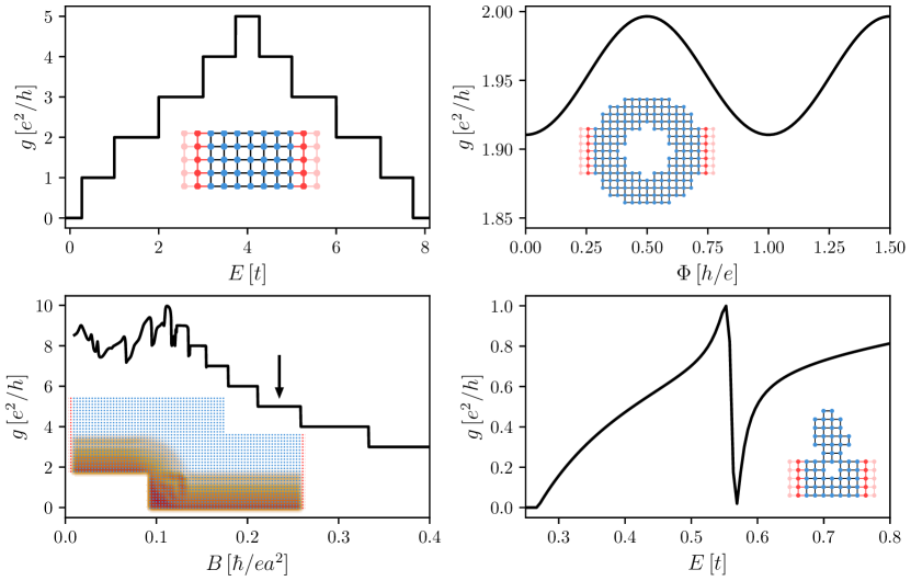
Figure 2: Examples of conductance calculations in a two dimensional square lattice. For each example the inset shows the tight-binding system that has been used with the scattering region in black and the first two layers of semi-infinite electrodes in red. Upper left: conductance quantization in a perfect ballistic quantum wire. Conductance $g$ is shown as a function of the Fermi energy $E$ expressed in units of the nearest-neighbor hopping strength $t$. Upper right: Aharonov-Bohm effect in a ring device threaded by magnetic flux $\Phi$. Lower left: quantum Hall effect in an example shape. The conductance is shown as a function of magnetic field in units of flux quanta per surface of a lattice unit cell ($a^{2}$). The inset displays the current density for one particular value of magnetic field which is indicated by the arrow. Lower right: Fano resonance in a quantum dot device.

II.7 Practical examples of numerical calculations

We end this pedagogical section with a few examples of practical systems that illustrate the kinds of calculations that can be made. We restrict these examples to toy models of simple devices made from a two-dimensional square lattice with a single orbital per site. More advanced examples involving more complex lattices (e.g., graphene), realistic modeling, multi-terminal devices, three dimensions, and treatment of internal degrees of freedom such as spin or particles and holes in superconductivity will be presented in the Secs. IX and X.

Figure 2 shows the conductance as a function of Fermi energy or magnetic field strength for four simple devices. The first device is a five sites wide perfect wire. Due to the translation invariance of the wire all the available conductance channels have perfect transmission $T_{a}=1$. Consequently, $g(E)$, shown in Fig. 2(a) has a staircase shape with the maximum number of propagating channels occurring in the middle of the band, where the corresponding infinite 2D system has a Van Hove singularity. Analyzing the number of open modes in a lead is a useful part of the workflow for setting up more complex calculations. The Hamiltonian matrix of this example has a simple graph structure that is displayed in the inset. The Hamiltonian itself is given by Eq. (22) with index $m$ running from $1$ to $5$ due to the finite system width.

A ring connected to two electrodes threaded by magnetic flux shown in Fig. 2(b) allows to study the Aharonov-Bohm effect. To account for the presence of magnetic flux $\phi\hbar/e$ through the hole, we modify the Hamiltonian hopping matrix elements $H_{nm}$ along a vertical line in the lower arm of the ring $H_{nm}\rightarrow e^{i\phi}H_{nm}$. Because of gauge invariance, the conductance does not depend on the position of the cut along which the hoppings are modified. Other than that and the shape of the scattering region, the Hamiltonian is again given by Eq. (22). The oscillations of the $g(\phi)$ demonstrate the Aharonov-Bohm effect.

A step-shaped sample in Fig. 2(c) is subject to a constant magnetic field, which brings it to the quantum Hall regime once the field is strong enough. This magnetic field prevents current from flowing through the middle of the sample, and creates edge states that carry current without backscattering [shown in the inset of Fig. 2(c)]. To include a vector potential in a tight-binding system we use the Peierls substitution [218, 115], which modifies the hopping according to

$$H_{nm}\to H_{nm}\exp\left[\mathrm{i}e/\hbar\int_{\bm{r}_{n}}^{\bm{r}_{m}}\bm{A}d\bm{r}\right].$$ (33)

We choose the vector potential in the Landau gauge with $\bm{B}=B\hat{z}$, so that $\bm{A}=-By\hat{x}$, so that the hoppings become

$$H_{nm}(\Phi)=H_{nm}(0)\times\mathrm{e}^{-\mathrm{i}\Phi(x_{n}-x_{m})(y_{n}+y_{m})/2},$$ (34)

with $\Phi=Bea^{2}/\hbar$ the magnetic flux per lattice unit cell in units of flux quanta, and $a$ the lattice constant. Note that we have chosen $\mathbf{A}$ such that $H_{nm}$ does not depend on $x$. This allows us to use the same gauge in $x$-directed electrodes while keeping the electrode Hamiltonian translation invariant.

A scattering setup with an irregular shape shown in the Fig. 2(d) emulates a quantum dot attached to a quantum wire. The dot traps a resonant level with energy $E_{0}$ and a lifetime $\Gamma$, so that interference between the direct transmission and resonant tunneling gives rise to the conductance $g(E)\sim|t_{d}+\Gamma/(E-E_{0}+i\Gamma)|^{2}$, with $t_{d}$ the amplitude of direct transmission. The conductance trace then has the characteristic asymmetric shape known as the Fano resonance [105, 62].

III Scattering formalism for discrete models

There are several equivalent descriptions of quantum transport that use the Green’s functions, wave functions, or the scattering matrix as the main tool. This review chooses the $\Psi S$-formalism as the starting point and defines everything in terms of the scattering wave functions and the associated scattering matrix $S$. This section provides a comprehensive description of the $\Psi S$-approach and includes several proofs that are scattered in the literature as well as some new material. The other mathematically equivalent approaches are derived as corollaries of the scattering approach in the later sections.

A generic system considered here is shown in Fig. 3. It consists of a central finite scattering region that has an arbitrary Hamiltonian. The scattering region is connected to a number of semi-infinite electrodes, each consisting of an infinite number of identical repeated unit cells.

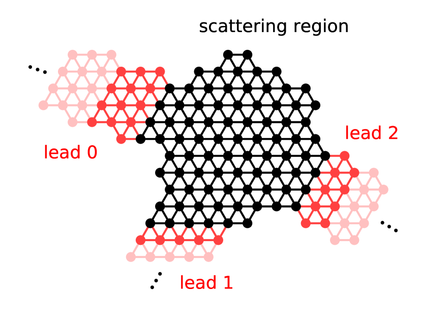
Figure 3: Schematic of a typical system for numerical simulations. The finite scattering region (black) is connected to semi-infinite, translationally invariant quasi-one dimensional electrodes (red). The dark- light-red colored cells correspond to the first and second unit cells of the semi-infinite leads respectively. Each lead can be at a different chemical potential and/or temperature.

III.1 Definition of the infinite lead problem

We first analyze the wave function in the translationally invariant region of the leads without considering the tight-binding equations of the scattering region. Each unit cell contains $N_{\mathrm{t}}$ sites and it has an onsite Hamiltonian matrix $H$ and the hopping matrix $V$ coupling one cell to the next. Grouping the degrees of freedom of the unit cells of multiple disconnected leads into a single vector defines a single larger lead with the Hamiltonian and the hopping being direct sums of the Hamiltonians and hoppings of the individual leads. Therefore without loss of generality we restrict our discussion to a single lead with the infinite Hamiltonian,

$$\hat{H}_{\text{lead}}=\begin{pmatrix}\ddots&\ddots&\ddots\\ &V&H&V^{\dagger}\\ &&V&H&V^{\dagger}\\ &&&V&H&V^{\dagger}\\ &&&&\ddots&\ddots&\ddots\\ \end{pmatrix},$$ (35)

and a wave function $\hat{\phi}=[\ldots,\hat{\phi}(j-1),\hat{\phi}(j),\hat{\phi}(j+1),\ldots]^{T}$. Because the tight-binding equations are translationally invariant, the wave function can be written as a superposition of the eigenvectors of translation operator, each of the form

$$\hat{\phi}(j)=\lambda^{j}\phi,$$ (36)

where the solutions with $\lambda\equiv e^{ik}$ and hence $|\lambda|=1$ are plane waves, $|\lambda|\neq 1$ are not normalizable and correspond to evanescent modes. Applied to a translation eigenvalue, the Schrödinger equation $\hat{H}_{\text{lead}}\hat{\phi}=E\hat{\phi}$ reads

$$V\phi+\lambda(H-E)\phi+\lambda^{2}V^{\dagger}\phi=0.$$ (37)

This is a quadratic eigenvalue problem for $\lambda$ and $\phi$ which has in general $2N_{\mathrm{t}}$ solutions for any energy $E$. Introducing $\xi\equiv\lambda\phi$ recasts Eq. (37) into a generalized eigenvalue problem

$$\begin{pmatrix}H-E&V^{\dagger}\\ 1&0\end{pmatrix}\begin{pmatrix}\phi\\ \xi\end{pmatrix}=\lambda^{-1}\begin{pmatrix}-V&0\\ 0&1\end{pmatrix}\begin{pmatrix}\phi\\ \xi\end{pmatrix}.$$ (38)

The inverse problem of Eq. (38) is finding the eigenvectors and eigenenergies of propagating waves with a given wave vector $k$:

$$H(k)\phi =E(k)\phi,$$ (39)

$$H(k) =H+e^{ik}V^{\dagger}+e^{-ik}V.$$ (40)

This defines the band structure of the lead with the bands $E_{\alpha}(k)$, found by stable numerical diagonalization of a hermitian matrix $H(k)$. The generalized eigenvalue problem Eq. (38), on the other hand, is not Hermitian, and therefore solving it in a numerically stable way is a nontrivial problem that we address in Sec. IV.

An example of dispersion relation of a $3$ sites lead is shown in Fig. 4. Note that for a given value of $k$ there always are $N_{\mathrm{t}}$ eigenenergies (here $3$). In contrast, for a given $E$ there are at most $2N_{\mathrm{t}}$ different propagating states. In the following, we suppose that we have found the different solutions of Eq. (37) at a given energy $E$ using the algorithms discussed later in this review.

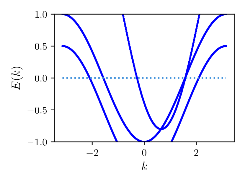
Figure 4: Example of a lead dispersion relation $E(k)$ in a simple situation where $H(k)$ is a $3\times 3$ matrix. For a given value of $k$, $H(k)$ always has $3$ eigenvalues. However for a given energy $E$, the number of different values of $k$ such that $E(k)=E$ can be strictly smaller than $6=3\times 2$. In this example for, e.g., $E=+0.75$ there are only $2\times 2$ values of $k$ ($2$ with $\partial E/\partial k>0$ and $2$ with $\partial E/\partial k<0$) which signifies the existence of evanescent states.

Solving the general eigenvalue problem Eq. (38) can be rather subtle if one wants to do it in a robust way, in particular when the matrix $V$ is not invertible. This problem has been discussed in a number of publications [242, 250, 92, 144, 135, 280, 206, 281, 121] and will be investigated in details below and in the next section. A close connection exists between the lead problem (of interest here) and the problem of calculating the properties of surfaces of metallic systems that uses a closely connected construction [8, 9, 156, 157, 284]

III.2 Separation of propagating and evanescent modes

After one has solved the general eigenvalue problem Eq. (38), the next step in the construction is to classify the different solutions $\phi_{\alpha}$ into propagating (p) and evanescent (e) modes, according to the value of $|\lambda|$: propagating for $|\lambda|=1$ and evanescent for $|\lambda|\neq 1$. Then, the propagating modes are further subclassified into outgoing (+) modes with positive velocity $v=(1/\hbar)dE/dk>0$ and incoming (-) modes with $v<0$. For normalized modes such that $\phi^{\dagger}\phi=1$, the mode velocity can be computed through Feynman-Hellman equation (see Appendix A for its derivation)

$$v=i\phi^{\dagger}\left[\lambda V^{\dagger}-\lambda^{-1}V\right]\phi$$ (41)

Note that there is always the same number $N_{\mathrm{p}}$ of incoming and outgoing propagating channels. This comes from the $2\pi$-periodicity and the continuity of the bands $E(k)$. Indeed, a horizontal line at a given energy $E$ must cross each band an even number of times, with half of the crossings at a positive slope and the other half with a negative slope, hence the equal number of modes with positive and negative velocities. For future convenience, we renormalize the propagating modes so that they carry unit velocity $\pm 1$. The same subclassification is applied to the $N_{\mathrm{e}}$ evanescent modes: outgoing (+) for those decaying at $+\infty$ ($|\lambda|<1$) and incoming (-) for the others ($|\lambda|>1$). The evanescent modes have zero velocities, and therefore their normalization may be chosen arbitrarily. As for propagating modes, the evanescent modes also appear in pairs: if $\lambda$ is a solution, then so is $1/\lambda^{*}$. Since the total number of incoming (or outgoing) modes is equal to the number of sites in a unit cell, we have $N_{\mathrm{t}}=N_{\mathrm{p}}+N_{\mathrm{e}}$.

The last step of this section is to gather the eigenstates $\phi_{\alpha}$ into a $N_{\mathrm{t}}\times 2N_{\mathrm{t}}$ matrix $\Phi$: the column $\alpha$ of $\Phi$ is a vector $\phi_{\alpha}$ or,

$$\Phi_{n\alpha}=(\phi_{\alpha})_{n}.$$ (42)

We further define the submatrices $\Phi_{\mathrm{p+}}$, $\Phi_{\mathrm{p-}}$,$\Phi_{\mathrm{e+}}$,$\Phi_{\mathrm{t+}}$…as the subblocks of $\Phi$ containing the corresponding modes. Similarly, we introduce the $2N_{\mathrm{t}}\times 2N_{\mathrm{t}}$ diagonal matrix $\Lambda$ that contains the eigenvalues $\lambda_{\alpha}$ on its diagonal. The submatrices $\Lambda_{\mathrm{p+}}$, $\Lambda_{\mathrm{p-}}$,…are its restriction to the corresponding modes. In some cases, we will exclude the modes that belong to the kernel of the matrix $V$ (i.e., such that $V\phi_{\alpha}=0$) and we note $\Phi_{\mathrm{\bar{t}+}}$, $\Lambda_{\mathrm{\bar{t}+}}$ the corresponding matrices. We note $\Phi_{\mathrm{o+}}$ the matrix that only contains those modes belonging to the kernel of $V$ ($V\Phi_{\mathrm{o+}}=0$). Keeping track of which modes are included in these matrices is central to all the various proofs and formula that are derived later in this article, so that we gather all these notations in Table 1 for future reference.

Symbol	Modes included	Size of the matrix	Direction
$\Phi_{\mathrm{p+}}$	propagating	$N_{\mathrm{t}}\times N_{\mathrm{p}}$	outgoing
$\Lambda_{\mathrm{p+}}$	propagating	$N_{\mathrm{p}}\times N_{\mathrm{p}}$	outgoing
$\Phi_{\mathrm{p-}}$	propagating	$N_{\mathrm{t}}\times N_{\mathrm{p}}$	incoming
$\Phi_{\mathrm{e+}}$	evanescent	$N_{\mathrm{t}}\times N_{\mathrm{e}}$	decaying away
$\Phi_{\mathrm{\bar{e}+}}$	evanescent except the $\lambda_{\alpha}=0$ modes	$N_{\mathrm{t}}\times N_{\mathrm{\bar{e}}}$	decaying away
$\Phi_{\mathrm{t+}}$	$\left(\Phi_{\mathrm{p+}}|\Phi_{\mathrm{e+}}\right)$: propagating & evanescent	$N_{\mathrm{t}}\times N_{\mathrm{t}}$	outgoing & decaying away
$\Phi_{\mathrm{\bar{t}+}}$	$\left(\Phi_{\mathrm{p+}}|\Phi_{\mathrm{\bar{e}+}}\right)$: propagating & evanescent, except $\lambda_{\alpha}=0$ modes	$N_{\mathrm{t}}\times N_{\mathrm{\bar{t}}}$	outgoing & decaying away
$\Phi_{\mathrm{t-}}$	$\left(\Phi_{\mathrm{p-}}|\Phi_{\mathrm{e+}}\right)$: propagating & evanescent	$N_{\mathrm{t}}\times N_{\mathrm{t}}$	incoming & decaying away
$\Phi_{\mathrm{\bar{t}-}}$	$\left(\Phi_{\mathrm{p-}}|\Phi_{\mathrm{\bar{e}+}}\right)$: propagating & evanescent, except $\lambda_{\alpha}=0$ modes	$N_{\mathrm{t}}\times N_{\mathrm{\bar{t}}}$	incoming & decaying away
$\Phi_{\mathrm{o+}}$	only the $\lambda_{\alpha}=0$ modes	$N_{\mathrm{t}}\times N_{\mathrm{o}}$	-

Table 1: Notations for the different modes in the electrodes. The letters stand respectively for evanescent (e), propagating (p) total (t), $\lambda_{\alpha}=0$ (o) and total without o modes ($\mathrm{\bar{t}}$). $+$ ($-$) indicates propagation or decay away from (towards) the scattering region. $N_{\mathrm{t}}=N_{\mathrm{p}}+N_{\mathrm{e}}=N_{\mathrm{\bar{t}}}+N_{\mathrm{o}}$ and $N_{\mathrm{e}}=N_{\mathrm{\bar{e}}}+N_{\mathrm{o}}$. Note that the evanescent modes $\Phi_{\mathrm{e-}}$ that are growing exponentially in the lead region are never needed in the calculations. The notation $\left(A|B\right)$ means stacking the columns of the $B$ matrix on the right of the columns of the $A$ matrix.

These matrices will be important ingredients of the construction of the scattering problem and allow one to express many things in a compact form. For instance, a general eigenstate of the lead Hamiltonian at a given energy can be written as a superposition of all modes which reads,

$$\hat{\phi}(j)=\Phi\Lambda^{j}q.$$ (43)

Here $q$ is a vector of size $2N_{\mathrm{t}}$. Using the submatrices, we can form less general states. For instance, a purely propagating state takes the form,

$$\hat{\phi}(j) = \Phi_{\mathrm{p}}(\Lambda_{\mathrm{p}})^{j}q_{\mathrm{p}}$$ (44)

$$= \Phi_{\mathrm{p+}}(\Lambda_{\mathrm{p+}})^{j}q_{\mathrm{p+}}+\Phi_{\mathrm{p-}}(\Lambda_{\mathrm{p-}})^{j}q_{\mathrm{p-}}$$

Using these matrices, Eq. (37) takes the form,

$$V\Phi+(H-E)\Phi\Lambda+V^{\dagger}\Phi\Lambda^{2}=0$$ (45)

III.3 Formulation of the Scattering problem as a set of linear equations

We now turn to the scattering problem per se: we connect the lead to a finite scattering region sr. The total system is now semi-infinite and is described by the Hamiltonian,

$$\hat{H}_{\text{sys}}=\begin{pmatrix}H_{\text{sr}}&P_{\text{sr}}^{T}V^{\dagger}\\ VP_{\text{sr}}&H&V^{\dagger}\\ &V&H&V^{\dagger}\\ &&V&H&V^{\dagger}\\ &&&\ddots&\ddots&\ddots\\ \end{pmatrix}$$ (46)

where $H_{\text{sr}}$ is the (big) $N_{\text{sr}}\times N_{\text{sr}}$ Hamiltonian of the scattering region. Without loss of generality, we have included the first layer of the lead inside the scattering region. Also, the multi-lead problem can be treated by using a larger effective lead. The coupling of the lead to the scattering region takes the specific form $VP_{\text{sr}}$ where the projector $P_{\text{sr}}$ is a $N_{\mathrm{t}}\times N_{\text{sr}}$ rectangular matrix with ones in the diagonal and zeros everywhere else.

We wish to calculate the scattering states $\hat{\psi}$ of $\hat{H}_{\text{sys}}$. We denote $\hat{\psi}$ in the scattering region $\psi_{\text{sr}}$. In the lead, the scattering states are formed by a combination of the incoming and outgoing propagating modes as well as the evanescent outgoing modes. The general form of $\hat{\psi}$ in the lead reads,

$$\hat{\psi}(j)=\Phi_{\mathrm{t+}}(\Lambda_{\mathrm{t+}})^{j}q_{\mathrm{t+}}+\Phi_{\mathrm{p-}}(\Lambda_{\mathrm{p-}})^{j}q_{\mathrm{p-}},$$ (47)

where the index $j>0$ labels the different lead unit cells. In other words, we seek wave functions of the form

$$\hat{\psi}=\begin{pmatrix}\psi_{\textrm{sr}}\\ \Phi_{\mathrm{t+}}\Lambda_{\mathrm{t+}}q_{\mathrm{t+}}+\Phi_{\mathrm{p-}}\Lambda_{\mathrm{p-}}q_{\mathrm{p-}}\\ \Phi_{\mathrm{t+}}(\Lambda_{\mathrm{t+}})^{2}q_{\mathrm{t+}}+\Phi_{\mathrm{p-}}(\Lambda_{\mathrm{p-}})^{2}q_{\mathrm{p-}}\\ \vdots\end{pmatrix}$$ (48)

The Schödinger equation $\hat{H}_{\text{sys}}\hat{\psi}=E\hat{\psi}$ imposes a linear relations between the incoming and outgoing modes - equivalent to the wave matching condition in the continuum - so that,

$$q_{\mathrm{t+}}=S_{\mathrm{tp}}q_{\mathrm{p-}}$$ (49)

where $S_{\mathrm{tp}}$ is the generalized scattering matrix. $S_{\mathrm{tp}}$ is a $(N_{\mathrm{p}}+N_{\mathrm{e}})\times N_{\mathrm{p}}$ matrix which extends the usual definition of the scattering matrix: it contains the outgoing propagating states as well as the outgoing evanescent ones. The usual scattering matrix $S\equiv S_{\mathrm{pp}}$ is recovered by taking the submatrix consisting of the $N_{\mathrm{p}}$ rows corresponding to outgoing propagating states.

Writing the Schödinger equation $\hat{H}_{\text{sys}}\hat{\psi}=E\hat{\psi}$ in terms of the decomposition Eq. (47), one arrives at a set of linear equation for $\psi_{\text{sr}}$ and $S_{\mathrm{tp}}$. Introducing the $N_{\text{sr}}\times N_{\mathrm{p}}$ matrix $\Psi_{\text{sr}}$ whose different columns contains the different solutions $\psi_{\text{sr}}$ corresponding to the different incoming propagating modes allows one to write the Schrödinger equation in a compact form. Using Eq. (45), we arrive at the following general formulation of the scattering problem:

$$\begin{pmatrix}H_{\text{sr}}-E&P_{\text{sr}}^{T}V^{\dagger}\Phi_{\mathrm{t+}}\Lambda_{\mathrm{t+}}\\ VP_{\text{sr}}&-V\Phi_{\mathrm{t+}}\end{pmatrix}\begin{pmatrix}\Psi_{\text{sr}}\\ S_{\mathrm{tp}}\end{pmatrix}=\begin{pmatrix}-P_{\text{sr}}^{T}V^{\dagger}\Phi_{\mathrm{p-}}\Lambda_{\mathrm{p-}}\\ V\Phi_{\mathrm{p-}}\end{pmatrix}$$ (50)

The problem is now formally reduced to solving a set of (usually very sparse) linear equations, which can be done very efficiently by various numerical packages.

III.4 Dealing with non-invertible hopping matrices

The linear system (50) becomes ill-conditioned when the hopping matrix $V$ is not invertible [242], i.e., when there are modes such that $V\Phi_{\mathrm{o,+}}=0$. In that case, the columns $\left(P_{\text{sr}}^{T}V^{\dagger}\Phi_{\mathrm{o+}}\Lambda_{\mathrm{o+}},-V\Phi_{\mathrm{o+}}\right)^{\dagger}$ in the left hand side of Eq. (50) become identical to zero. This is due to the fact that the $\Phi_{\mathrm{o+}}$-modes do not contribute explicitly to the scattering wave function. Instead, we should formulate the problem in terms of the modes $\Phi_{\mathrm{\bar{t}+}}$.

If this is done naively in Eq. (50), the matrix on the left-hand side becomes rectangular, and the linear system is thus overdetermined. We can however return to a square matrix by introducing the singular value decomposition of $V=U_{A}DU_{B}^{\dagger}$ where $U_{A}$ and $U_{B}$ are unitary matrices and the diagonal matrix $D$ contains $N_{\mathrm{\bar{t}}}$ non-zero singular values. Defining $A=U_{A}\sqrt{D}$, $B=U_{B}\sqrt{D}$ and reshaping these matrices to keep only their non-zero part, we arrive at

$$V=AB^{\dagger}$$ (51)

where $A$ and $B$ are $N_{\mathrm{t}}\times N_{\mathrm{\bar{t}}}$ matrices of orthogonal vectors.

With this decomposition we find

$$\begin{pmatrix}H_{\text{sr}}-E&P_{\text{sr}}^{T}V^{\dagger}\Phi_{\mathrm{\bar{t}+}}\Lambda_{\mathrm{\bar{t}+}}\\ AB^{\dagger}P_{\text{sr}}&-AB^{\dagger}\Phi_{\mathrm{\bar{t}+}}\end{pmatrix}\begin{pmatrix}\Psi_{\text{sr}}\\ S_{\mathrm{tp}}\end{pmatrix}=\begin{pmatrix}-P_{\text{sr}}^{T}V^{\dagger}\Phi_{\mathrm{p-}}\Lambda_{\mathrm{p-}}\\ AB^{\dagger}\Phi_{\mathrm{p-}}\end{pmatrix}.$$ (52)

Noticing that the last rows are multiplied by $A$, we find that any solution of

$$\begin{pmatrix}H_{\text{sr}}-E&P_{\text{sr}}^{T}V^{\dagger}\Phi_{\mathrm{\bar{t}+}}\Lambda_{\mathrm{\bar{t}+}}\\ B^{\dagger}P_{\text{sr}}&-B^{\dagger}\Phi_{\mathrm{\bar{t}+}}\end{pmatrix}\begin{pmatrix}\Psi_{\text{sr}}\\ S_{\mathrm{tp}}\end{pmatrix}=\begin{pmatrix}-P_{\text{sr}}^{T}V^{\dagger}\Phi_{\mathrm{p-}}\Lambda_{\mathrm{p-}}\\ B^{\dagger}\Phi_{\mathrm{p-}}\end{pmatrix}.$$ (53)

is thus a valid solution of the scattering problem. Eq. (53) is the most generic formulation of the scattering problem, and we will use it in the majority of this review. The name of the $\Psi S$-approach derives from the fact that one solves simultaneously for $\Psi_{\text{sr}}$ and $S_{\mathrm{tp}}$.

III.5 Formulation of the bound state problem

Besides the states that hybridize with the continuum spectrum of the leads, there can also be bound states that decay in the leads. Those are usually outside of the leads bands, but not necessarily (a trivial example being a non connected system or different symmetries between the scattering region and the leads). An important example of bound states are the Andreev states that form in a normal region sandwiched by superconducting leads. Another example are the edge states at the boundary of topological insulators.

The general form of $\hat{\psi}(j)$ for a bound state reads,

$$\hat{\psi}(j)=\Phi_{e+}(\Lambda_{e+})^{j}q_{e+}$$ (54)

for $j>0$ (in the lead) and $\psi_{\text{sr}}$ in the scattering region. With these notations and a bit of algebra described in [118], the Schrödinger equation translates into

$$\begin{pmatrix}H_{\text{sr}}-E&P_{\text{sr}}^{T}V^{\dagger}\Phi_{\mathrm{e+}}\Lambda_{e+}\\ \Lambda_{e+}^{*}\Phi_{e+}^{\dagger}VP_{\text{sr}}&-\Lambda_{e+}^{*}\Phi_{e+}^{\dagger}V\Phi_{e+}\end{pmatrix}\begin{pmatrix}\psi_{\text{sr}}\\ q_{e+}\end{pmatrix}=0,$$ (55)

The matrix $\Lambda_{e+}$ can contain zero diagonal elements, which gives Eq. (55) spurious solutions at every energy $E$. We then introduce the matrices $\Lambda_{\mathrm{\bar{e}+}}$, where we keep only the non zero eigenvalues, as well as $\Phi_{\mathrm{\bar{e}+}}$ and $q_{\mathrm{\bar{e}+}}$, whose columns corresponding to the zero eigenvalue have been discarded, to obtain the correct formulation of the problem

$$\begin{pmatrix}H_{\text{sr}}-E&P_{\text{sr}}^{T}V^{\dagger}\Phi_{\mathrm{\bar{e}+}}\Lambda_{\mathrm{\bar{e}+}}\\ \Lambda_{\mathrm{\bar{e}+}}^{*}\Phi_{\mathrm{\bar{e}+}}^{\dagger}VP_{\text{sr}}&-\Lambda_{\mathrm{\bar{e}+}}^{*}\Phi_{\mathrm{\bar{e}+}}^{\dagger}V\Phi_{\mathrm{\bar{e}+}}\end{pmatrix}\begin{pmatrix}\psi_{\text{sr}}\\ q_{\mathrm{\bar{e}+}}\end{pmatrix}=0.$$ (56)

Although Eq. (56) looks similar to Eq. (50) they are structurally different: there is no source term of the right hand side of Eq. (56) so that we cannot simply solve a linear system. In the scattering problem, the energy $E$ is known and one seek the solutions at that given energy, here we must first find the values of $E=E_{\mathrm{BS}}$ for which the matrix on the left hand side of Eq. (56) becomes singular. For such an energy value, one looks for the corresponding kernel to find $\psi_{\text{sr}}$ and $q_{\mathrm{\bar{e}+}}$. Since $\Phi_{\mathrm{\bar{e}+}}$ and $\Lambda_{\mathrm{\bar{e}+}}$ depends on energy $E$, computing the bound state energies amounts to finding the roots of a non-linear function while computing the associated eigenstate is pure linear algebra [118].

In the particular case of a semi-infinite wire with no scattering region, $H_{\text{sr}}$ is simply replaced by $H$, $P_{\text{sr}}$ by the identity and $\psi_{\text{sr}}=\Phi_{\mathrm{\bar{e}+}}\Lambda_{\mathrm{\bar{e}+}}q_{\mathrm{\bar{e}+}}$. In that case, Eq. (56) can be recast in the form,

$$V\Phi_{\mathrm{\bar{e}+}}q_{\mathrm{\bar{e}+}}=0$$ (57)

which implies that the matrix $V\Phi_{\mathrm{\bar{e}+}}$ does not have full rank.

III.6 Discrete symmetries and conservation laws

The scattering matrix $S$ together with the definition of the scattering modes $\Phi$ describe single energy properties of an infinite system (46), and therefore it is constrained by the symmetries of the Hamiltonian. Taking explicitly these symmetries into account when solving for the leads is necessary to obtain certain physical observables. For instance, defining a spin-resolved conductance between two normal leads requires keeping track of the spin degree of freedom in the lead. Similarly, calculating the Andreev conductance of a normal metal-superconductor junction requires keeping track of the conserved electron/hole degree of freedom in the normal lead. In the same spirit, to compute topological invariants, one must take into account the discrete symmetry class of the system. This subsection discusses possible strategies to make use of the symmetries in numerical calculations.

Because $S$ is a map between the two vector spaces spanned by the columns of $\Phi_{p-}$ and $\Phi_{p+}$, it transforms differently from linear operators. Specifically, applying unitary transformations $\Phi^{\prime}_{p-}=\Phi_{p-}U_{p-}$, $\Phi^{\prime}_{p+}=\Phi_{p+}U_{p+}$ transforms $S$ into $S^{\prime}=U_{p+}^{\dagger}SU_{p-}$. One strategy would be to describe how the symmetry constraints apply to the scattering matrix for an arbitrary choice of the basis $\Phi$. Instead, here we utilize the arbitrariness of this choice to choose the symmetry-adapted basis where the action of symmetries on $S$ assumes a simple form, as implemented in the Kwant package [104].

III.6.1 Conservation laws

Unitary symmetries are associated with conservation laws such as the conservation of spin. As these conservation laws are associated with directly observable quantities, they are relatively straightforward to take into account. We consider a conserved quantity in a lead. It is given by a Hermitian operator $\hat{A}$, that commutes with the lead Hamiltonian. More specifically, we suppose that $\hat{A}$ takes the form of a block diagonal translationally invariant operator described by a matrix $A$ inside one unit cell:

$$\hat{A}=\begin{pmatrix}&\ddots&\\ &0&A&0\\ &&0&A&0\\ &&&0&A&0\\ &&&&&\ddots&\\ \end{pmatrix}.$$ (58)

It satisfies $[H,A]=[V,A]=0$. For instance, the conservation of the spin along the z axis is implemented by the choice of $A=\sigma_{z}$ where the Pauli matrix $\sigma_{z}$ acts in the spin sector. The lead Hamiltonian leaves the eigensubspaces of $\hat{A}$ decoupled, and therefore any lead mode belongs to a single eigensubspace of $\hat{A}$. Let $U^{i}$ be an orthonormal set of eigenvectors for the eigenvalue $a_{i}$ of $A$:

$$A=\sum_{i}U^{i}a_{i}U^{i\dagger},$$ (59)

we can defined the lead problem projected onto the $i$-th eigensubspace of $\hat{A}$ in terms of the two matrices

$$H_{i} =U^{i\dagger}HU^{i}$$ (60)

$$V_{i} =U^{i\dagger}VU^{i}$$ (61)

with the number of degrees of freedom per unit cell equal to the degeneracy of $a_{i}$. Each of the sub-lead problem for the symmetry sector $i$ is then solved separately to obtain the associated lead modes $\Phi_{i}$. Then, we obtain the full solution by just combining the $\Phi_{i}$ with the $U^{i}$ using,

$$\Phi=\sum_{i}U^{i}\Phi_{i}.$$ (62)

III.6.2 Discrete symmetries

In addition to unitary symmetries that are associated with conservation laws, Hamiltonians may possess some of the discrete symmetries: time-reversal $\mathcal{T}$, particle-hole $\mathcal{P}$, and sublattice or chiral symmetry $\mathcal{C}$. These symmetries are antiunitary ($\mathcal{T}$ and $\mathcal{P}$) and/or antisymmetries ($\mathcal{P}$ and $\mathcal{C}$). Antiunitary symmetries are defined as the product of a unitary matrix with the complex conjugate operator; they flip the sign of the momentum of propagating modes. Antisymmetries anticommute with the Hamiltonian instead of commuting with it; they change the sign of the mode energy. These operators do not allow a simultaneous eigendecomposition with the Hamiltonian and require a separate treatment.

In the following, we focus on the case where the antiunitary symmetry operators take a form where $\mathcal{T}^{2}=\pm 1$ and $\mathcal{P}^{2}=\pm 1$, and the chiral symmetry to a form such that $\mathcal{C}^{2}=1$. It can indeed be shown [287] that it is always possible to construct such symmetries (or more precisely a form where all the eigenvalues of $\mathcal{T}^{2}$ and $\mathcal{P}^{2}$ are $\pm 1$ together with $\mathcal{C}^{2}=1$.)

To see why such a construction is possible and illustrate how one can take advantage of symmetries practically, let’s consider the example where only the time reversal symmetry is present: $\mathcal{T}=UK$ where $U$ is a unitary matrix acting on the unit cell of the lead and $K$ the complex conjugation operator. One immediately obtains that $\mathcal{T}^{2}=Q\equiv U^{*}U$, i.e., $\mathcal{T}^{2}$ is a regular unitary symmetry $Q$ that commutes with the Hamiltonian as well as with $\mathcal{T}$. Let us diagonalize $Q$ first and consider an eigenstate $\mathbf{q}$ with eigenvalue $e^{iq}$, i.e., $Q\mathbf{q}=e^{iq}\mathbf{q}$. We find that $\mathcal{T}\mathbf{q}$ is also an eigenstate of $Q$ with eigenvalue $e^{-iq}$. If $q=0$ or $\pi$ then we have $\mathcal{T}^{2}\mathbf{q}=\pm\mathbf{q}$ and the construction of the new time-reversal operator $\mathcal{T^{\prime}}$ is trivial in this sector: $\mathcal{T^{\prime}}=\mathcal{T}$. In all other situations, $e^{-iq}\neq e^{iq}$ and the two states $\mathbf{q}$ and $\mathcal{T}\mathbf{q}$ are orthogonal. Now, we define a new unitary matrix $R$ inside the space spanned by $\mathbf{q}$ and $\mathcal{T}\mathbf{q}$ by $R\mathbf{q}=e^{-iq}\mathbf{q}$ and $R\mathcal{T}\mathbf{q}=\mathcal{T}\mathbf{q}$. From $R$, we can define a new time-reversal operator $\mathcal{T^{\prime}}=R\mathcal{T}$. This new operator is obviously the product of a unitary matrix $RU$ times $K$ and commutes with the Hamiltonian, hence it is a proper time-reversal operator. It is easy to verify that it satisfies $\mathcal{T^{\prime}}^{2}\mathbf{q}=\mathbf{q}$ and $\mathcal{T^{\prime}}^{2}\mathcal{T}\mathbf{q}=\mathcal{T}\mathbf{q}$, i.e., that $\mathcal{T^{\prime}}^{2}=1$ which proves our statement.

These discrete symmetries act on the Bloch Hamiltonian as follows:

$$\mathcal{T}H(\bm{k})\mathcal{T}^{-1} =H(-\bm{k}),$$ (63a)

$$\mathcal{P}H(\bm{k})\mathcal{P}^{-1} =-H(-\bm{k}),$$ (63b)

$$\mathcal{C}H(\bm{k})\mathcal{C}^{-1} =-H(\bm{k}).$$ (63c)

Since $\hbar v=\partial E/\partial k$, $\mathcal{T}$ and $\mathcal{C}$ flip the sign of $v$, while $\mathcal{P}$ leaves it unchanged. It follows that $\mathcal{T}$ and $\mathcal{C}$ can be used to define the outgoing modes from the incoming ones.

III.6.3 Construction of the lead modes using discrete symmetries

The strategy to take advantage of the discrete symmetries is to use the symmetries in the construction of the modes. Whenever a discrete symmetry maps one propagating mode onto another, we define one of the two modes in the pair by applying the symmetry operator to the other one. More precisely, we use the symmetries (if present!) in the following order: if a conservation law exists, it is used first, as described in the previous section. Second we use $\mathcal{T}$ that allows one to define the outgoing modes from the incoming ones. Third, only at $E=0$, we can use $\mathcal{P}$ which allows to define the modes with negative $-\pi<k<0$ from the mode with positive $0<k<\pi$. Last, only at $E=0$, the $\mathcal{C}$ symmetry provides the outgoing mode from the incoming one.

If a discrete symmetry coexists with a conservation law $\hat{A}$, it must map an eigensubspace of $\hat{A}$ onto another eigensubspace of $\hat{A}$, possibly the same one [287]. If different eigensubspaces are related by one or more discrete symmetries, we define the modes $\Phi$ in one of these subspaces by applying the discrete symmetry $\mathcal{T}$, $\mathcal{P}$, and/or $\mathcal{C}$ (in the order defined above) to the modes in the other subspace.

When $\mathcal{P}^{2}=-1$, its presence guarantees a Kramers-like degeneracy of propagating modes with the same velocity at $E=0$ for the high symmetry momenta $k=0$ and $k=\pi$. We determine pair of modes related by particle-hole symmetry at these momenta by selecting an arbitrary mode $\phi$, computing its particle-hole partner $\mathcal{P}\phi$, and projecting the remaining modes at this momentum onto the subspace orthogonal to this pair.

When $\mathcal{P}^{2}=1$ at a high symmetry momentum $k=0$ or $k=\pi$ and $E=0$, we cannot use the strategy of choosing the wave function of one mode in a pair by acting with the symmetry on another mode. To implement a symmetry-adapted basis in this case, we choose the mode wave functions such that they are mapped by $\mathcal{P}$ onto themselves. To do so, we compute the action of $\mathcal{P}$ within the space of modes with the same velocity at a high symmetry momentum: $\Omega=\Phi^{\dagger}\mathcal{P}\Phi$. Transforming $\Phi\rightarrow\Phi\Omega^{1/2}$ through a diagonalization of the $\Omega$ matrix achieves the desired result $\phi=\mathcal{P}\phi$ at a high symmetry momentum.

The combination of the presence/absence of different symmetries gives rise to many possible scenarios for the properties of the obtained scattering matrix using the above construction [93]. As an example, in the case where only time reversal symmetry is present, without additional conservation law, one arrives at

$$S_{\mathrm{pp}}=\mathcal{T}^{2}S_{\mathrm{pp}}^{T}$$ (64)

Similarly the presence of the chiral symmetry alone leads to,

$$S_{\mathrm{pp}}(E=0)=\mathcal{T}^{2}S_{\mathrm{pp}}^{\dagger}$$ (65)

. The presence of a global particle-hole symmetry $\mathcal{P}=\tau_{x}K$ present in the Bogoliubov-De-Gennes equation for superconductors (here $\tau_{x}$ is the Pauli matrix acting in the Nambu electron-hole space) combined with the conservation law $A=\tau_{z}$ (e.g., charge is conserved in a non-superconducting lead) leads to the following useful form for transport across superconducting systems,

$$S_{\mathrm{pp}}(E=0)=\mathcal{P}^{2}S_{\mathrm{pp}}^{*}.$$ (66)

More complex situations may arise when combining symmetries in yet different ways.

III.7 Other related wave function approaches

There are many closely related ways one can calculate the scattering wave functions and in this review, we have focused on the one used in the Kwant package [104] developed by some of us. Historically, the wave function approach was pioneered in the work of [15] who integrated out the leads degrees of freedom to obtain

$$[E-H_{\text{sr}}-P_{\text{sr}}^{T}\Sigma P_{\text{sr}}]\Psi_{\text{sr}}=P_{\text{sr}}^{T}V^{\dagger}\Phi_{\mathrm{p}-}\Lambda_{\mathrm{p}-}-P_{\text{sr}}^{T}\Sigma\Phi_{\mathrm{p}-}.$$ (67)

From the perspective of this review, the Ando approach lies half way between the $\Psi S$-approach and the Green function approach. A natural derivation of this equation will be done in Sec. V where we will introduce the self energy matrix $\Sigma(E)$. Variations of this technique has been implemented by several groups in different contexts such as metallic spintronics [135] or constrictions [314].

IV Stable formulation of the lead and scattering problems

The purpose of this section is to design a stable algorithm to find the solutions of the generalized quadratic equation (37) and construct the matrices $\Phi$ and $\Lambda$ that are needed for the scattering problem.

Quadratic equations like Eq. (37),

$$V\Phi+\lambda(H-E)\Phi+\lambda^{2}V^{\dagger}\Phi=0$$ (68)

can be recast into generalized eigenvalue problems with the simple change of variable $\xi\equiv\lambda\Phi$:

$$\begin{pmatrix}H-E&V^{\dagger}\\ 1&0\end{pmatrix}\begin{pmatrix}\Phi\\ \xi\end{pmatrix}=\lambda^{-1}\begin{pmatrix}-V\Phi\\ \xi\end{pmatrix}$$ (69)

Note that we have formulated the eigenproblem in terms of $\lambda^{-1}$ since we are interested in $|\lambda|\leq 1$, and eigensolvers find large eigenvalues better than small ones. General eigensolvers are not always stable however, and the rest of this section is devoted to the derivation of a robust formulation of the problem.

IV.1 Simple case: $V$ is invertible

In the simplest situation, the matrix $V$ is invertible. Multiplying the first line of Eq. (69) with $V^{-1}$, we arrive at an ordinary eigenproblem,

$$\begin{pmatrix}-V^{-1}(H-E)&-V^{-1}V^{\dagger}\\ 1&0\end{pmatrix}\begin{pmatrix}\Phi\\ \xi\end{pmatrix}=\lambda^{-1}\begin{pmatrix}\Phi\\ \xi\end{pmatrix}$$ (70)

that can therefore be solved by usual linear algebra routines. Although this case might appear to be rather generic, there are many important examples, e.g., graphene, where the matrix $V$ is not invertible.

IV.2 Eigendecomposition in the general case

If the hopping matrix $V$ is not full invertible, the matrix on the left hand side of Eq. (69)) is singular, and often is ill-conditioned. Moreover, solving the generalized eigenproblem (69) also yields the solutions $\Phi_{o+}$ such that $V\Phi_{o+}=0$. In fact, every singular value of $V$ gives rise to an eigenvalue $\lambda=0$ and $\lambda=\infty$ in the generalized eigenproblem. However, the modes $\Phi_{o+}$ do not contribute to the scattering problem as we observed in Sec. III.3. Computing them explicitly is thus unnecessary and inefficient.

We can use the decomposition introduced in Eq. (51), $V=AB^{\dagger}$, with $A$ and $B$ $N_{\mathrm{t}}\times N_{\bar{\mathrm{t}}}$ matrices of orthogonal vectors, to alleviate both problems. With this decomposition, we can now rewrite equation (68) into the following form,

$$(E-H)(\lambda\Phi)=A(B^{\dagger}\Phi)+\lambda B(\lambda A^{\dagger}\Phi)$$ (71)

which is naturally expressed in terms of the variables $\Phi_{A}$ and $\Phi_{B}$ that we shall use from now on:

$$\Phi_{A}=\lambda A^{\dagger}\Phi\quad,\quad\Phi_{B}=B^{\dagger}\Phi$$ (72)

The next step is to express $\lambda\Phi$ in terms of $\Phi_{A}$ and $\Phi_{B}$. Since $E-H$ is not necessarily invertible, we first add a self-energy like term $+i(AA^{\dagger}+BB^{\dagger})(\lambda\Phi)$ on both sides of Eq. (71). This term shifts the eigenvalues of $H$ away from the real axis guaranteeing that the matrix $E-H+i(AA^{\dagger}+BB^{\dagger})$ is always invertible except when $H-E$ and $V$ have a joint zero eigenvector (or in other words that there is a flat band at exactly the energy $E$). The problem now reads,

$$\left[E-H+i(AA^{\dagger}+BB^{\dagger})\right](\lambda\Phi)=$$

$$(\lambda B+iA)\Phi_{A}+(A+i\lambda B)\Phi_{B}.$$ (73)

Introducing

$$G_{AB}=\left[E-H+i(AA^{\dagger}+BB^{\dagger})\right]^{-1}$$ (74)

we get,

$$\lambda\Phi=G_{AB}(\lambda B+iA)\Phi_{A}+G_{AB}(A+i\lambda B)\Phi_{B}.$$ (75)

Last, multiplying Eq. (75) by $A^{\dagger}/\lambda$ and $B^{\dagger}/\lambda$ we arrive at a the following eigenvalue problem that only involves $\Phi_{A}$ and $\Phi_{B}$,

$$\begin{pmatrix}A^{\dagger}G_{AB}B&iA^{\dagger}G_{AB}B\\ -B^{\dagger}G_{AB}B&1-iB^{\dagger}G_{AB}B\end{pmatrix}\begin{pmatrix}\Phi_{A}\\ \Phi_{B}\end{pmatrix}=\frac{1}{\lambda}\begin{pmatrix}1-iA^{\dagger}G_{AB}A&-A^{\dagger}G_{AB}A\\ iB^{\dagger}G_{AB}A&B^{\dagger}G_{AB}A\end{pmatrix}\begin{pmatrix}\Phi_{A}\\ \Phi_{B}\end{pmatrix}$$ (76)

Eq. (76)) provides a stable generalized eigenproblem that can be solved with standard linear algebra routine. Additionally, this generalized eigenproblem (76) is smaller than the one in Eq. (69): $2N_{\bar{\mathrm{t}}}\times 2N_{\bar{\mathrm{t}}}$ instead of $2N_{\mathrm{t}}\times 2N_{\mathrm{t}}$. Eq. (76)) is used in particular in the Kwant package[104]. Alternative techniques to reduce the eigenproblem in the case of singular hopping matrices have been developed in Refs. [242, 248].

IV.3 Link with the scattering problem

Let us now go back to the scattering problem Eq. (50). The scattering problem can be rewritten in term of the $\Phi_{A}$ and $\Phi_{B}$ matrices only,

$$\begin{pmatrix}H_{\text{sr}}-E&P_{\text{sr}}^{T}B\Phi_{A,\mathrm{t+}}\\ AB^{\dagger}P_{\text{sr}}&-A\Phi_{B,\mathrm{t+}}\end{pmatrix}\begin{pmatrix}\Psi_{\text{sr}}\\ S_{\mathrm{tp}}\end{pmatrix}=\begin{pmatrix}-P_{\text{sr}}^{T}B\Phi_{A,\mathrm{p-}}\\ A\Phi_{B,\mathrm{p-}}\end{pmatrix}$$ (77)

The left hand side Eq. (77) has some columns that are purely zero in the case where V is not invertible. Indeed, in this case, the corresponding $\Phi_{A}$ vanishes while $V\Phi=0$ implies that $A\Phi_{B}=0$. To proceed, we simply remove these columns from Eq. (77). The resulting matrix is now rectangular, i.e., we have an over complete set of equations. To restore a square matrix, we remove the $A$ matrices from the second line and arrive at,

$$\begin{pmatrix}H_{\text{sr}}-E&P_{\text{sr}}^{T}B\Phi_{A,\mathrm{\bar{t}+}}\\ B^{\dagger}P_{\text{sr}}&-\Phi_{B,\mathrm{\bar{t}+}}\end{pmatrix}\begin{pmatrix}\Psi_{\text{sr}}\\ S_{\mathrm{\bar{t}p}}\end{pmatrix}=\begin{pmatrix}-P_{\text{sr}}^{T}B\Phi_{A,\mathrm{p-}}\\ \Phi_{B,\mathrm{p-}}\end{pmatrix}$$ (78)

Any solution of Eq. (78) automatically satisfies Eq. (77). In a last step, we slightly modify Eq. (78) in order to make the left hand side better conditioned for numerical purposes. Indeed, one observes that in some situations the columns of the matrix

$$\begin{pmatrix}\Phi_{A,\mathrm{\bar{e}+}}\\ \Phi_{B,\mathrm{\bar{e}+}}\end{pmatrix}$$ (79)

can be nearly linearly dependent due to the eigenvalue problems (70) and (76) being non-Hermitian. In that case the matrix of the left-hand side of Eq. (78) is ill-conditioned [306]. To avoid performing an unstable eigenvalue decomposition, we use the generalized Schur decomposition (QZ decomposition) [100] of the Eq. (76) instead. The transformation performs a joined decomposition of a pair of matrices (matrix pencil) as $(X,Y)=(QSZ^{\dagger},QTZ^{\dagger})$, with matrices $Q$ and $Z$ unitary and $S$ and $T$ upper triangular. The diagonal entries of $S$ and $T$ are related to the eigenvalues of the generalized eigenproblem $X\psi=\lambda Y\psi$ by $\lambda_{i}=S_{ii}/T_{ii}$. In other words, the first vectors of the $Z$ matrix form an orthogonal basis in the eigensubspace corresponding to the first eigenvalues appearing on the diagonals of $S$ and $T$. We then use standard LAPACK functions to extract the eigenvectors corresponding to propagating modes from the Schur decomposition, as well as an orthogonal basis corresponding to the evanescent modes. This is equivalent, to performing a QR decomposition of the wave functions of the evanescent modes, i.e., by reorthogonalizing the evanescent eigenstates:

$$\begin{pmatrix}\Phi_{A,\mathrm{\bar{e}+}}\\ \Phi_{B,\mathrm{\bar{e}+}}\end{pmatrix}=\begin{pmatrix}Q_{A,\mathrm{\bar{e}+}}\\ Q_{B,\mathrm{\bar{e}+}}\end{pmatrix}R,$$ (80)

however it avoids an unstable step of obtaining the eigenvectors $\Phi_{\mathrm{\bar{e}+}}$ from the eigenvalue problem Eq. (76). Furthermore, obtaining a subset of the eigenvectors from Schur does not introduce a computational overhead because the Schur decomposition is performed by LAPACK as the first step of solving the generalized eigenvalue problem anyway. Using the orthogonal basis for the evanescent states, we arrive at the following $2\times 3$ block structure which forms our final form of the scattering problem.

$$\begin{pmatrix}H_{\text{sr}}-E&P_{\text{sr}}^{T}B\Phi_{A,\mathrm{\bar{p}+}}&P_{\text{sr}}^{T}BQ_{A,\mathrm{\bar{e}+}}\\ B^{\dagger}P_{\text{sr}}&-\Phi_{B,\mathrm{\bar{p}+}}&-Q_{B,\mathrm{\bar{e}+}}\\ \end{pmatrix}\begin{pmatrix}\Psi_{\text{sr}}\\ S_{\mathrm{pp}}\\ RS_{\mathrm{\bar{e}p}}\end{pmatrix}$$

$$=\begin{pmatrix}-P_{\text{sr}}^{T}B\Phi_{A,\mathrm{p-}}\\ \Phi_{B,\mathrm{p-}}\end{pmatrix}$$ (81)

Practical calculations, for instance in the Kwant package, are performed by numerically solving the linear system Eq. (81).

IV.4 Diagonalization of current operator and proper modes

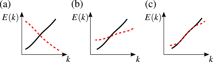
Figure 5: Different scenarios for the band structure $E(k)$ that give rise to degenerate eigenvalues $\lambda_{i_{n}}$ for the mode eigenproblem in Eqs. (70) and (76).

The mode eigenproblems in Eqs. (70) and (76) may have degenerate eigenvalues $\lambda_{i_{n}}$ (with $n=1,\dots,N_{\text{deg}}$, where $N_{\text{deg}}$ is the degeneracy). In this case, any linear superposition of eigenvectors is also an eigenvector, and in general numerical algorithms will indeed return an arbitrary superposition.

For propagating modes, $\lambda_{i_{n}}=e^{ik}$ with real $k$, this corresponds to a crossing or degeneracy of bands $E(k)$ at a given value of $k$. A couple of scenarios given rise to this situation are shown in Fig. 5. This case needs special treatment:

• In the derivation of the Landauer–Büttiker formula in Sec. II.3 we need to assume that the scattering states are orthogonal. This also requires that the lead eigenstates are orthogonal, and for lead modes with the same $k$, this implies that $\phi_{i_{n}}$ need to form an orthogonal set. Additionally, the derivation Landauer–Büttiker formula requires that the lead modes diagonalize the current operator. This follows automatically for modes corresponding to different $\lambda_{i}\neq\lambda_{j}$, (see App. B), but not for degenerate $\lambda_{i_{n}}$.

• For both Landauer–Büttiker and the definition of retarded Green’s function in Sec. V.1 we need to reliably separate in- and outgoing propagating modes. To this end need the velocity of a numerically computed mode to be continuous. This is also guaranteed by imposing the condition of modes $\phi_{i_{n}}$ being orthogonal and diagonalizing the current operator, as both conditions are true away from the degeneracy point and result in modes that are unique up to a phase, if the velocities $v_{i_{n}}$ are all different.

The algorithm is thus as follows: Let $\Phi_{\mathrm{p},\text{deg}}$ be the $N_{\mathrm{t}}\times N_{\text{deg}}$ matrix consisting of eigenvectors of Eqs. (70) and (76) corresponding to the degenerate eigenvalue $\lambda_{i_{n}}$ with $|\lambda_{i_{n}}|=1$. We first find an orthogonal basis for the space spanned by the eigenvectors using a QR decomposition:

$$\Phi_{\mathrm{p},\text{deg}}=Q_{\mathrm{p},\text{deg}}R\,.$$ (82)

We then use this orthogonal basis to compute the $N_{\text{deg}}\times N_{\text{deg}}$ velocity matrix

$$\mathcal{V}=iQ_{\mathrm{p},\text{deg}}^{\dagger}(\lambda_{i_{n}}V^{\dagger}-\lambda_{i_{n}}V)Q_{\mathrm{p},\text{deg}}$$ (83)

Being Hermitian, $\mathcal{V}$ c can be diagonalized with real eigenvalues as

$$U^{\dagger}\mathcal{V}U=\begin{pmatrix}v_{i_{1}}&&\\ &\ddots&\\ &&v_{i_{N_{\text{deg}}}}\end{pmatrix}\,.$$ (84)

$\bar{\Phi}_{\mathrm{p},\text{deg}}=Q_{\mathrm{p},\text{deg}}U$ then forms an orthogonal set of propagating modes that diagonalizes the current operator, as demanded by the requirements above. This procedure has to be repeated for every cluster of degenerate eigenvalues corresponding to a propagating mode.

V Green’s function formalism for the quantum problem

In the preceding sections, we have introduced quantum transport from the point of view of the scattering matrix formalism. The scattering matrix approach expresses the quantum transport problem as a waveguide problem which is very appealing conceptually. In particular, it provides a natural explanation for the quantization of conductance. It is also a very effective formulation for numerical purposes, since, as we have seen, it allows one to map the problem to the solution of a (sparse) linear problem. In this section, we introduce another, yet fully equivalent, formalism in terms of Green’s functions. In fact, the Green’s functions approach was introduced first and was for a long time the preferred approach for numerics through the celebrated “recursive Green’s function” algorithm.

This section contains an introduction to the Green’s function approach and to its connection with the scattering formalism. We focus here on the retarded Green’s function which can be put in direct correspondence with the scattering matrix: the retarded Green’s function provides the amplitude for the propagation between two sites while the scattering matrix gives the amplitude for the propagation between two lead modes. We defer to Sec. VIII the derivation of the Non Equilibrium Greens Function (NEGF) formalism that allows one to calculate the actual physical observables from the knowledge of the retarded Green’s function.

In Sec. V.1 we first provide the general definitions of Green’s functions. Since electron-electron interactions are only considered at the mean-field level in this review, we restrict ourselves to quadratic Hamiltonians for which Green’s functions take a much simpler form. Sec. V.2 shows how the retarded Green’s function can be obtained from the solution of a linear problem similar to the one defined in the preceding sections for the scattering matrix. We proceed in Sec. V.3 and V.4 with defining the self-energy of a lead, an important concept of the Green’s function approach. Very interestingly, we shall find that the self-energy satisfies a self-consistent equation that could allow one to calculate it without the construction of the lead modes. In fact, self-energies are often calculated this way. The relation between the retarded Green’s function and the scattering matrix, known as the Fisher–Lee relation, is worked out in Sec. V.5. We end with Sec. V.6 where we discuss general relations that unveil common mathematical structures that occur in different parts of the formalism.

V.1 Definitions of Green’s functions

The Fourier transform $\hat{G}(E)$ of the retarded Green function takes the general formal form

$$\hat{G}(E)=\int dt\hat{G}(\tau)e^{iE\tau}=\lim_{\eta\rightarrow 0}\frac{\hat{1}}{E+i\eta-\hat{H}_{\text{sys}}}$$ (85)

where the real-time retarded Green’s function is defined as

$$\hat{G}(\tau)=i\Theta(t)e^{-i\hat{H}_{\text{sys}}\tau}.$$ (86)

Equivalently, one can define the retarded Green’s function in energy directly as the solution of the following equation:

$$[(E+i\eta)\hat{1}-\hat{H}_{\text{sys}}]\hat{G}(E)=\hat{1}.$$ (87)

Note that Eq. (87) does not have a unique solution and one should remember the presence of the infinitely small positive imaginary energy $\eta>0$ to properly define the retarded Green’s function. Computing $\hat{G}(E)$ is the central problem of Green’s function based methods.

In the following, we follow a route very similar to the one taken to define the scattering matrix. This allows us to obtain the Green’s function as the solution of a set of linear equations and also to obtain a direct connection between the Green’s function and the scattering matrix (referred as the Fisher–Lee relation). A different, more traditional route makes no reference to the scattering problem and makes use of the Dyson equation to calculate the retarded Green’s function directly. This route will be followed in the next section. It is completely equivalent to the first.

V.2 General formulation as a linear problem

Having defined the retarded Green’s function, our first task is to show that it can be obtained through the solution of a linear system very similar to the one that defines the Scattering matrix. Let us define $G(j,k)$ as the various subblocks of $\hat{G}(E)$ on the different unit cells (we keep the energy $E$ as implicit). Remember that $j>0$ corresponds to the semi-infinite leads and $j=0$ to the scattering region. Let us further suppose that we are only interested in $G(j,0)$ and mostly in $G_{\text{sr}}\equiv G(0,0)$. Writing explicitly the block structure of Eq. (87) gives

$$[E+i\eta-H_{\text{sr}}]G_{\text{sr}}-P^{T}_{\text{sr}}V^{\dagger}G(1,0)=1,$$ (88)

$$-VP_{\text{sr}}G_{\text{sr}}+[E+i\eta-H]G(1,0)-V^{\dagger}G(2,0)=0,$$ (89)

$$-VG(j-1,0)+[E+i\eta-H]G(j,0)-V^{\dagger}G(j+1,0)=0$$ (90)

where the last equation holds for $j>1$. Eq. (90) is in fact identical to the equation found for $\Psi(j)$ so that a decomposition similar to Eq. (47) applies. To keep the problem normalizable, only decaying and propagating modes can contribute. However, the presence of the small imaginary $\eta$ means that also propagating modes now become either decaying or growing exponentially away from the scattering region. This can be seen by considering $\lambda_{\alpha}=\lambda_{\alpha}(E)=e^{ik_{\alpha}(E)}$ as a function of complex energy and perform a Taylor expansion,

$$\begin{split}k_{\alpha}(E+i\eta)=&k_{\alpha}(E)+i\frac{dk_{\alpha}(E)}{dE}\eta+\mathcal{O}(\eta^{2})\\ =&k_{\alpha}(E)+\frac{i\eta}{\hbar v_{\alpha}(E)}+\mathcal{O}(\eta^{2}),\end{split}$$ (91)

where $v_{\alpha}=\frac{1}{\hbar}\frac{dE}{dk}$ is the velocity of the mode. Hence, all outgoing propagating modes with $v_{\alpha}>0$ become decaying ($\eta>0$ implies $|e^{ik_{\alpha}(E+i\eta)}|<1$), and we can write

$$G(j,0)=\Phi_{\mathrm{t}+}(\Lambda_{\mathrm{t}+})^{j}G_{\mathrm{t}+}$$ (92)

where the matrix $G_{\mathrm{t}+}$ sets the weight associated to the corresponding modes. Note that the advanced Green’s function $G^{A}=G^{\dagger}$ is defined by adding a small negative contribution $-i\eta$ to the energy $E$. The advanced Green’s function would thus involve the incoming modes $\Phi_{\mathrm{p-}}$ and the evanescent modes $\Phi_{\mathrm{e+}}$ (which together form $\Phi_{\mathrm{t-}}$ as defined in Table 1).

Following the same calculation as for the scattering problem, we arrive at a linear problem similar to Eq. (50):

$$\begin{pmatrix}E-H_{\text{sr}}&-P^{T}_{\text{sr}}V^{\dagger}\Phi_{\mathrm{t}+}\Lambda_{\mathrm{t}+}\\ -VP_{\text{sr}}&V\Phi_{\mathrm{t}+}\end{pmatrix}\begin{pmatrix}G_{\text{sr}}\\ G_{\mathrm{t}+}\end{pmatrix}=\begin{pmatrix}1\\ 0\end{pmatrix}$$ (93)

where the role of the “source” is now taken by the identity matrix (in site space) instead of the different incoming modes. Note that we can already now take the limit of $\eta\rightarrow 0$ in this finite matrix problem, as we already used $\eta$ to choose the contributing modes in the leads. If $V$ is non-invertible, we arrive in analogy to the wave function in Eq. (53) at

$$\begin{pmatrix}E-H_{\text{sr}}&-P^{T}_{\text{sr}}V^{\dagger}\Phi_{\mathrm{\bar{t}}+}\Lambda_{\mathrm{\bar{t}}+}\\ -B^{\dagger}P_{\text{sr}}&B^{\dagger}\Phi_{\mathrm{\bar{t}}+}\end{pmatrix}\begin{pmatrix}G_{\text{sr}}\\ G_{\mathrm{\bar{t}}+}\end{pmatrix}=\begin{pmatrix}1\\ 0\end{pmatrix}.$$ (94)

Both linear systems can be solved directly by standard numerical methods.

V.3 Self-energy of the leads

Our next step to make contact with the standard formulation of the Green’s function approach is to introduce the self-energy of the lead, i.e., to eliminate the $G_{\mathrm{\bar{t}}+}$ matrix in Eq. (94). From the second row of this equation, we find

$$G_{\mathrm{\bar{t}}+}=\frac{1}{B^{\dagger}\Phi_{\mathrm{\bar{t}}+}}B^{\dagger}P_{\textrm{sr}}G_{\textrm{sr}}.$$ (95)

The matrix $B^{\dagger}\Phi_{\mathrm{\bar{t}}+}$ is invertible, unless the energy corresponds to a bound state of the semi-infinite lead. This can only happen for discrete values of the energy $E$. The proof of this statement can be found in Appendix C.

Inserting (95) into the first row of Eq. (94), we arrive at

$$\left[E-H_{\text{sr}}-P^{T}_{\text{sr}}\Sigma(E)P_{\text{sr}}\right]G_{\text{sr}}=1,$$ (96)

i.e., the retarded Green’s function is simply given by the inverse of the scattering region Hamiltonian to which one has added a self-energy term $\Sigma=\Sigma(E)$. Here we have introduced the self-energy as

$$\Sigma=V^{\dagger}\Phi_{\mathrm{\bar{t}}+}\Lambda_{\mathrm{\bar{t}}+}\frac{1}{B^{\dagger}\Phi_{\mathrm{\bar{t}}+}}B^{\dagger}.$$ (97)

The above equation can be simplified further by noticing that $\frac{1}{B^{\dagger}\Phi_{\mathrm{\bar{t}}+}}B^{\dagger}\Phi_{\mathrm{\bar{t}}+}=1$ and $\frac{1}{B^{\dagger}\Phi_{\mathrm{\bar{t}}+}}B^{\dagger}\Phi_{\mathrm{o}+}=0$. Hence,

$$\frac{1}{B^{\dagger}\Phi_{\mathrm{\bar{t}}+}}B^{\dagger}=1_{\mathrm{\bar{t}\times t}}\Phi_{\mathrm{t}+}^{-1}$$ (98)

with

$$\mathrm{1}_{\mathrm{\bar{t}\times t}}=\left(\begin{array}[]{cccc|cc}\makebox[0.0pt][l]{$\smash{\overbrace{\phantom{\begin{matrix}1&0&0&\cdots\end{matrix}}}^{N_{\mathrm{\bar{t}}}}}$}1&0&0&\cdots&\makebox[0.0pt][l]{$\smash{\overbrace{\phantom{\begin{matrix}0&\cdots\end{matrix}}}^{N_{\mathrm{o}}}}$}0&\cdots\\ 0&1&0&&\vphantom{\int^{0}}\smash[t]{\vdots}\\ 0&0&1&&\\ \vphantom{\int^{0}}\smash[t]{\vdots}&&&\ddots&\\ \end{array}.\right)$$ (99)

In other words, $\frac{1}{B^{\dagger}\Phi_{\mathrm{\bar{t}}+}}B^{\dagger}$ is equal to the first $N_{\mathrm{\bar{t}}}$ rows of $\Phi_{\mathrm{t}+}^{-1}$. Since $\Phi_{\mathrm{\bar{t}}+}\Lambda_{\mathrm{\bar{t}}+}1_{\mathrm{\bar{t}\times t}}=\Phi_{\mathrm{t}+}\Lambda_{\mathrm{t}+}$, we thus find

$$\Sigma=V^{\dagger}\Phi_{\mathrm{t}+}\Lambda_{\mathrm{t}+}(\Phi_{\mathrm{t}+})^{-1}$$ (100)

Note that Eq. (100) is valid for both invertible and non-invertible hopping matrices.

The retarded Green’s function $G(i,j)$ has the asymptotic behavior (92) of only outgoing modes in the lead. The advanced Green’s function $G^{\dagger}(i,j)$ can be obtained in the same fashion, but now with an asymptotic behavior of only incoming modes in the lead. From this we find

$$\Sigma^{\dagger}=V^{\dagger}\Phi_{\mathrm{t}-}\Lambda_{\mathrm{t}-}(\Phi_{\mathrm{t}-})^{-1}.$$ (101)

Let us now consider the surface Green’s function $G_{\text{lead}}$ of a standalone semi-infinite lead (i.e., before it is connected to the scattering region). By surface, we mean the diagonal part of the Green’s function on the last unit cell. No additional calculation is required to obtain $G_{\text{lead}}$, it is a particular case of Eq. (96) where $H_{\text{sr}}$ is replaced with $H$:

$$\left[E-H-\Sigma\right]G_{\text{lead}}=1,$$ (102)

or alternatively can be defined as a linear system similar to Eq. (93). Our last goal for this subsection is to show that $G_{\text{lead}}$ and the self-energy $\Sigma$ are very simply related.

Using Eq. (45) one can rewrite the Eq. (100) above as

$$\Sigma\Phi_{\mathrm{t}+}\Lambda_{\mathrm{t}+}=(E-H)\Phi_{\mathrm{t}+}\Lambda_{\mathrm{t}+},-V\Phi_{\mathrm{t}+}$$ (103)

from which one gets

$$\Phi_{\mathrm{t}+}\Lambda_{\mathrm{t}+}=G_{\text{lead}}V\Phi_{\mathrm{t}+},$$ (104)

and eventually at the sought-after connection,

$$\Sigma=V^{\dagger}G_{\text{lead}}V.$$ (105)

Eq. (105) can be seen as a generalization of the Fermi golden rule. Its importance stems from the fact that we now have a closed set of equations (96), (102) and (105) that does not make use of the mode decomposition in terms of $\Phi_{\mathrm{t}+}$ and $\Lambda_{\mathrm{t}+}$, hence can be amenable to calculations through a different class of algorithms. From this perspective, one can see Eq. (104) as an eigenvector problem for the matrix $G_{\text{lead}}V$ which provides an implicit definition for $\Phi_{\mathrm{t}+}$ and $\Lambda_{\mathrm{t}+}$. In this review we have chosen to emphasize the “constructive approach” that starts from the scattering problem, and construct the Green function approach as its consequence. The alternative approach when one first defines the Green’s function is fully equivalent.

V.4 Properties of the linewidth $\Gamma$

Let’s introduce the linewidth matrix $\Gamma$ that plays an important role in the Green’s function formalism. It is a Hermitian matrix defined as

$$\Gamma=i\left[\Sigma-\Sigma^{\dagger}\right].$$ (106)

Multiplying the above equation by $\Phi_{\mathrm{t}+}^{\dagger}$ ($\Phi_{\mathrm{t}+}$) on the left (right), we find using Eq. (100) that

$$\Phi_{\mathrm{t}+}^{\dagger}\Gamma\Phi_{\mathrm{t}+}=i\left[\Phi_{\mathrm{t}+}^{\dagger}V^{\dagger}\Phi_{\mathrm{t}+}\Lambda_{\mathrm{t}+}-\Lambda_{\mathrm{t}+}^{*}\Phi_{\mathrm{t}+}^{\dagger}V\Phi_{\mathrm{t}+}\right].$$ (107)

We recognize the expressions for the velocity calculated in Eqs. (239), (240), (241) and (244) from which it follows that $\Phi_{\mathrm{p}+}^{\dagger}\Gamma\Phi_{\mathrm{p}+}=1$, while all the other blocks vanish $\Phi_{\mathrm{p}+}^{\dagger}\Gamma\Phi_{\mathrm{e}+}=\Phi_{\mathrm{e}+}^{\dagger}\Gamma\Phi_{\mathrm{p}+}=\Phi_{\mathrm{e}+}^{\dagger}\Gamma\Phi_{\mathrm{e}+}=0$. Introducing the diagonal matrix $\mathrm{1}_{\mathrm{p}}$ whose diagonal entries are unity for the propagating $\mathrm{p}$ sector and zero for the evanescent $\mathrm{e}$ sector, we therefore arrive at the very compact expression,

$$\Gamma=(\Phi_{\mathrm{t}+}^{\dagger})^{-1}\mathrm{1}_{\mathrm{p}}(\Phi_{\mathrm{t}+})^{-1},$$ (108)

from which one can directly get

$$\Gamma=\Gamma\Phi_{\mathrm{t}+}\Phi_{\mathrm{t}+}^{\dagger}\Gamma=\Gamma\Phi_{\mathrm{p}+}\Phi_{\mathrm{p}+}^{\dagger}\Gamma\,,$$ (109)

where the last equality follows from $\Gamma\Phi_{\mathrm{e}+}=0$, as evident from Eq. (108). Similar expressions can be obtained for incoming modes. Indeed, they satisfy $\Sigma^{\dagger}(E)\Phi_{\mathrm{t}-}=V^{\dagger}\Phi_{\mathrm{t}-}\Lambda_{\mathrm{t}-}$. Following the same route as above, and using Eq. (245) one arrives at

$$\Gamma=(\Phi_{\mathrm{t}-}^{\dagger})^{-1}\mathrm{1}_{\mathrm{p}}(\Phi_{\mathrm{t}-})^{-1},$$ (110)

from which one can directly get

$$\Gamma=\Gamma\Phi_{\mathrm{t}-}\Phi_{\mathrm{t}-}^{\dagger}\Gamma=\Gamma\Phi_{\mathrm{p}-}\Phi_{\mathrm{p}-}^{\dagger}\Gamma.$$ (111)

Eqs. (109) and (111) are central for showing the equivalence of the Green’s function and scattering wave function approach.

V.5 Fisher–Lee relation

The Landauer–Büttiker formula derived in Sec. II.3 relates the conductance to the intuitive scattering formalism. In the following section we derive an expression that demonstrates the equivalence of the scattering approach to the Green’s function formalisms, originally demonstrated in [87].

From the second row of Eq. (53), we find

$$\begin{split}S_{\mathrm{\bar{t}p}}&=\frac{1}{B^{\dagger}\Phi_{\mathrm{\bar{t}}+}}B^{\dagger}\left(P_{\text{sr}}\Psi_{\text{sr}}-\Phi_{\mathrm{p-}}\right)\\ &=1_{\mathrm{\bar{t}\times t}}\Phi_{\mathrm{t}+}^{-1}\left(P_{\text{sr}}\Psi_{\text{sr}}-\Phi_{\mathrm{p-}}\right).\end{split}$$ (112)

Inserting this into the first row of Eq. (53) we then arrive at an equation for the wave function $\Psi_{\text{sr}}$,

$$(E-H_{\text{sr}}-P_{\text{sr}}^{T}\Sigma P_{\text{sr}})\Psi_{\text{sr}}=P_{\text{sr}}^{T}\left(V^{\dagger}\Phi_{\mathrm{p-}}\Lambda_{\mathrm{p-}}-\Sigma\Phi_{\mathrm{p-}}\right),$$ (113)

where we used Eq. (97). In Eq. (113), we recognize the Ando mixed wavefunction approach introduced in Sec. III.7.

From Eq. (96) we know that $G_{\text{sr}}=\left(E-H_{\text{sr}}-P_{\text{sr}}^{T}\Sigma P_{\text{sr}}\right)^{-1}$. Additionally, from Eq. (101) we have $\Sigma^{\dagger}(E)\Phi_{\mathrm{p-}}=V^{\dagger}\Phi_{\mathrm{p-}}\Lambda_{\mathrm{p-}}$. Hence,

$$\Psi_{\text{sr}}=iG_{\text{sr}}P_{\text{sr}}^{T}\Gamma\Phi_{\mathrm{p-}}.$$ (114)

Inserting this identity back into Eq. (112), we find

$$S_{\mathrm{\bar{t}p}}=\mathrm{1}_{\mathrm{\bar{t}\times t}}\Phi_{\mathrm{t+}}^{-1}\left[iP_{\text{sr}}G_{\text{sr}}P^{T}_{\text{sr}}\Gamma-1\right]\Phi_{\mathrm{p-}}.$$ (115)

Equation (115) is a generalization of the original Fisher–Lee relations that connect the retarded Green’s function to the scattering matrix. If we restrict the scattering matrix to only propagating modes, we can use the fact that $\Phi_{\mathrm{p+}}^{\dagger}\Gamma=1_{\mathrm{p\times t}}\Phi_{\mathrm{t+}}^{-1}$ to simplify this expression further to obtain

$$S_{\mathrm{pp}}=\Phi_{\mathrm{p+}}^{\dagger}\left[i\Gamma P_{\text{sr}}G_{\text{sr}}P^{T}_{\text{sr}}\Gamma-\Gamma\right]\Phi_{\mathrm{p-}}.$$ (116)

V.6 Common underlying structure of the site elimination problem

The Fisher–Lee relation is a particular example of a family of relations. In this subsection, we identify common mathematical patterns in the different algebraic routes that have been followed so far. This subsection does not contain new material but rather offer a global point of view on various operations and algorithms that might look disconnected at first sight.

Our starting point is a general tight-binding equation that connects two subsystems $1$ and $2$. It corresponds to one line of the Schrödinger equation written in block form and is therefore under-determined,

$$H_{11}\Psi_{1}+H_{12}\Psi_{2}=0,$$ (117)

where $H_{11}$ is a square matrix (that incorporates the energy $E$ for concision) and $H_{12}$ is rectangular. Since we cannot fully solve it, we will rather express the value of some variables in terms of others.

The first step is to write a low-rank representation of $H_{12}$ using, e.g., a singular value decomposition. $H_{12}$ factorizes as $H_{12}=AB^{\dagger}$ and we further introduce $\Psi_{A}=A^{\dagger}\Psi_{1}$, $\Psi_{B}=B^{\dagger}\Psi_{2}$. It is straightforward to find that these two vectors are related through,

$$\Psi_{A}=-A^{\dagger}\frac{1}{H_{11}}A\Psi_{B}$$ (118)

To continue, we want to choose a “double” basis on which we will decompose $\Psi_{A}$ and $\Psi_{B}$. We refer to the first basis as “known” and the second one as “unknown”, we will see some concrete examples below. The different vectors of these bases are stacked together so that the block matrix

$$\Phi=\begin{pmatrix}\Phi^{\textrm{kn}}_{A}&\Phi^{\textrm{un}}_{A}\\ \Phi^{\textrm{kn}}_{B}&\Phi^{\textrm{un}}_{B}\\ \end{pmatrix}$$ (119)

forms a basis for the vector $(\Psi_{A},\Psi_{B})^{T}$. Now searching for the solution of Eq. (117) of the form $\Psi_{A/B}=\Phi^{\textrm{un}}_{A/B}S-\Phi^{\textrm{kn}}_{A/B}$ where the $S$ matrix is some sort of generalized scattering matrix, we arrive at

$$\begin{pmatrix}H_{11}&A\Phi_{B}^{\textrm{un}}\\ -A^{\dagger}&\Phi_{A}^{\textrm{un}}\end{pmatrix}\begin{pmatrix}\Psi_{1}\\ S\end{pmatrix}=\begin{pmatrix}A\Phi_{B}^{\textrm{kn}}\\ \Phi_{A}^{\textrm{kn}}\end{pmatrix}.$$ (120)

Eq. (120) is very general and accounts for many familiar situations depending on how one splits the system and which basis is used for the decomposition between known and unknown states.

The first example is for the actual scattering matrix of the system. In that case $\Psi_{2}$ refers to the leads, the “unknown” basis corresponds to the output states and the “known” to the input. However Eq. (120) is not limited to this case. For instance, choosing $\Phi^{\textrm{un}}_{A}=\Phi^{\textrm{kn}}_{B}=I_{d}$ and $\Phi^{\textrm{un}}_{B}=\Phi^{\textrm{kn}}_{A}=0$, we arrive at $\Sigma=BSB^{\dagger}$ where $\Sigma$ is the self-energy due to subsystem $1$ on the sites of subsystem $2$. A third example is the transfer matrix $M$ of the system. Suppose that we equip the space spanned by $\Psi_{A}$ and $\Psi_{B}$ with a left/right block structure (this structure might actually correspond to parts of subsystem $2$ situated on the left and on the right of subsystem $1$, but this definition is more general). Then we choose $\Phi^{\textrm{kn}}_{A}=\Phi^{\textrm{un}}_{B}=1_{L}\oplus 0_{R}$ and $\Phi^{\textrm{un}}_{A}=\Phi^{\textrm{kn}}_{B}=0_{L}\oplus 1_{R}$, where $1_{L/R}$ ($0_{L/R}$) is the identity (null) matrix acting on the left/right. The obtained $S$ from this partition is actually the transfer matrix $M$ of the system. More examples could be constructed in the same way. For instance, one may define virtual modes that are eigenstates of the current operator. The associated virtual leads would allow one to split the study of the system into two (or more) regions that are recombined at the end. This could be advantageous when one part of the system needs to be updated more often than the other (e.g., the disordered part for statistics) or in the presence of a bottleneck in the system (e.g., a quantum point contact). A possible choice for this is $\Phi^{\textrm{un}}_{A}=\Phi^{\textrm{kn}}_{A}=I_{d}$ and $\Phi^{\textrm{un}}_{B}=-\Phi^{\textrm{kn}}_{B}=iI_{d}$.

The above construction has the advantage to automatically provide the Fisher–Lee relations between different objects. Indeed, the knowledge of $S$ allows one to compute

$$A^{\dagger}H_{11}^{-1}A=-\left(\Phi^{\textrm{un}}_{A}S-\Phi^{\textrm{kn}}_{A}\right)\left(\Phi^{\textrm{un}}_{B}S-\Phi^{\textrm{kn}}_{B}\right)^{-1},$$ (121)

and in return the knowledge of $A^{\dagger}H_{11}^{-1}A$ allows one to compute $S$ in a potentially different basis,

$$S=\left(\Phi^{\textrm{un}}_{A}+A^{\dagger}H_{11}^{-1}A\Phi^{\textrm{un}}_{B}\right)^{-1}\left(\Phi^{\textrm{kn}}_{A}+A^{\dagger}H_{11}^{-1}A\Phi^{\textrm{kn}}_{B}\right).$$ (122)

Inserting Eq. (121) with $S$ and $\Phi$ into Eq. (122) for a different splitting $S^{\prime}$ and $\Phi^{\prime}$ provides a cumbersome yet fully explicit “Fisher–Lee” relation between $S$ and $S^{\prime}$.

VI Numerical algorithms

We have now introduced two equivalent formalisms, the $\Psi S$ scattering wavefunction and the Green function formalism. The initially infinite eigenvector problem $\hat{H}_{\text{sys}}\hat{\psi}=E\hat{\Psi}$ has been cast onto a finite linear problem of the form $Ax=b$ where $A$ is a large sparse matrix. Solving this problem numerically amounts to doing some sort of Gaussian elimination for which there are various strategies.

In this section, we go through the main algorithms that have been developed to solve the quantum transport problem. In Sec. VI.1 we comment on how to solve the lead problem that enters into the linear system. Sec. VI.2 discusses using direct sparse solvers to solve a general quantum transport problem, and why these solvers are often the method of choice. Sec. VI.3 introduces the Dyson equation, an effective tool for practical calculations of the retarded Green’s function, and the basis of many Green’s function-based algorithms. Sec. VI.4 uses it for explaining the original recursive Green’s function algorithm and its extensions. We end this section with a broader discussion, in VI.5 of a wide range of algorithms used in quantum transport including those that do not fully fit within the Green’s function or the scattering matrix approach.

VI.1 The lead problem

All the central formulas of this review, such Eq. (53) for computing the scattering wave function or Eqs. (96) and (100) to compute the Green’s function, rely on first computing the lead modes.

If a lead has a simple structure it may be possible to determine the corresponding $\phi$ and $\lambda$ analytically. One such example is a square lattice with only a single orbital [71]. In the general case however, it is necessary to follow the procedure outlined in Sec. IV. In particular, this involves solving the (generalized) eigenproblems in Eqs. (70) and (76), as well as the singular value decomposition of the matrix $V$. For each of these problems there are standard routines in LAPACK [14]. Several implementations of LAPACK and BLAS also allow for parallelization through OpenMP.

Solving the (generalized) eigenproblem of a dense matrix with LAPACK yields all eigenvalues and -vectors. Recent works have employed contour-integral methods to only compute eigenvalues close in a finite region around the unit circle, an approach that also is amenable to parallelization [155, 120, 121].

Before using eigenproblems to compute lead modes was established, the self-energy or surface Green’s function of the lead was often computed iteratively [175]. In this approach, repeated doubling of the lead unit cell gives a fast convergence towards a truly semi-infinite lead (this scheme is related to the recursive Green’s function method described in Sec. VI.4). However, it requires the introduction of a small but finite imaginary part $\eta$ to the energy $E\rightarrow E+i\eta$. Hence, it requires some fine tuning to perform the calculations with high accuracy [288].

VI.2 Solving the linear system of Eq. (53)

Eq. (53) (and (94) for the Green’s function) are typically sparse linear systems of equations. The direct, numerical solution of sparse linear systems has been studied extensively in the past decades (for a comprehensive review see [72, 74]). For the solution of the quantum transport problem, we can heavily lean on these developments. In fact, there are several publicly available software packages of direct solvers, such as MUMPS [12, 11], UMFPACK [73], or SuperLU [166].

The crucial step in solving a sparse system of linear equations is a sparse $LU$-decomposition of the coefficient matrix. The time and memory required for this task depends directly on the number of non-zeros in the factors $L$ and $U$. It is known that fill-in, i.e., additional non-zeros in $L$ and $U$ compared to the original coefficient matrix, depends crucially on the order of decomposition, and thus on the ordering of the coefficient matrix [74]. Many different heuristic algorithms for finding fill-in-reducing orderings have been developed, such as approximate minimum degree ordering [10] or nested dissection [99, 169]. Several of these heuristic algorithms are distributed with the direct sparse solver packages mentioned above, or are available as separate software packages, such as Metis [129] or SCOTCH [219].

Out of these, nested dissection is particularly interesting for sparse linear systems arising from a real-space discretization. For example, it has been shown [99] for a two-dimensional $M\times M$ square grid that solving the linear system of equations takes $\mathcal{O}(M^{3})$ operations and $\mathcal{O}(M^{2}\log(M))$ storage, a scaling that has been shown to be optimal [114]. For comparison, the traditional recursive Green’s function algorithm needs $\mathcal{O}(M^{4})$ operations and $\mathcal{O}(M^{3})$ storage for the same problem (see Sec. VI.4). In fact, for practical examples, using direct sparse solvers was shown to be significantly faster than the recursive Green’s function algorithm [176, 40], and scaling more favorably [104].

We derived Eqs. (67) and (96) by eliminating parts of the unknowns in Eqs. (53) and (94). It may seem advantageous to solve these smaller linear systems instead. However, the self-energy $\Sigma$ entering these equations can diverge (see Sec. V.3), although the original systems are well-behaved. It is thus advantageous to rather solve Eqs. (53) and (94), as direct sparse solvers use pivoting to enhance numerical stability. If only a part of the solution is needed, it can be advantageous to use sparse methods to compute a Schur complement directly [168].

Historically, dedicated solvers have been developed to solve the quantum transport problem. However, for a general problem – with arbitrary structure – direct sparse solvers are superior to dedicated solvers in terms of numerical stability, flexibility and efficiency, given the amount of research in that field. Hence, a direct sparse solver often is the method of choice, e.g., in Kwant [104]. Still, taking into account the explicit structure of a specific problem can be advantageous and reduce, e.g., memory requirements or overhead, and in the following we review such approaches.

VI.3 Dyson equation and the gluing sequence

The set of equations (96), (102) and (105) is very appealing because it reduces the task of finding the inverse of a infinite matrix to the inverse of a finite one (96) together with the self-consistent equations (102) and (105).

We now introduce Dyson equation, which provides a practical route for such a calculation. We do not consider here the original Dyson equation of quantum field theory, but a much weaker form that rather belongs to linear algebra. In this section we switch to notations that use Gothic letters such as $\mathds{H}$ or $\mathds{G}$. A matrix $\mathds{H}$ may refer to the actual Hamiltonian matrix $H$ but more likely will refer to a sub-block of certain matrix elements of it. For instance, it may be the Hamiltonian matrix of certain sites in the absence of certain hopping matrix elements. Many such matrices need to be considered in an actual algorithm.

Suppose that we split an Hamiltonian $\mathds{H}$ into two parts $\mathds{H}=\mathds{H}_{0}+\mathds{H}_{1}$ (usually referred to as the unperturbed Hamiltonian and the perturbation) and want to calculate the Green’s function $\mathds{G}=1/(E-\mathds{H})$. We further suppose that $\mathds{G}_{0}=1/(E-\mathds{H}_{0})$ is already known. Elementary algebra shows that

$$\mathds{G}=\mathds{G}_{0}+\mathds{G}_{0}\mathds{H}_{1}\mathds{G}=\mathds{G}_{0}+\mathds{G}\mathds{H}_{1}\mathds{G}_{0}$$ (123)

(as proved by multiplying Eq. (123) by $E-\mathds{H}$). Equation (123) is known as the Dyson equation.

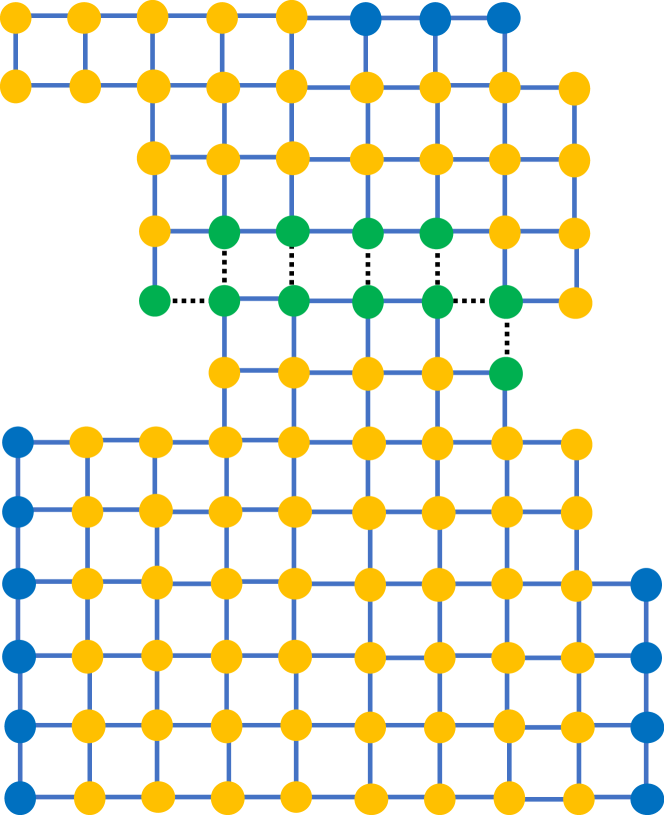
Figure 6: Schematic of the “gluing sequence” that uses the Dyson equation to incorporate new matrix elements (symbolized by the dotted black lines) into the calculation. The first step of the calculation involves only the (green) “connected” sites that are directly affected by the new matrix elements. In the second and last steps, one updates the Green’s function for the blue sites, a subset of all the possible sites. the interest of Dyson equation stems from the fact that only the blue and green sites are involved in the calculation.

Its power originates from the fact that one can often choose the matrix $\mathds{H}_{1}$ such that $(\mathds{H}_{1})_{mn}\neq 0$ only for a small number of “connected” sites $m,n$. The Dyson equation projected onto these connected sites gives a closed set of equations. Hence, it is not necessary to invert the (potentially infinite) matrix $E-\mathds{H}$ but a much smaller version.

In particular, the Dyson equation can be used in a three step process to “glue” together two parts of a system that are initially disconnected, see a cartoon in Fig. 6. Introducing the superscript C (green sites) and D (blue and orange sites) for the corresponding connected and disconnected blocks (i.e., sites belonging or not to the group of connected sites), one finds that Eq. (123) takes a closed form for the CC block,

$$\mathds{G}^{\text{CC}}=\mathds{G}_{0}^{\text{CC}}+\mathds{G}_{0}^{\text{CC}}\mathds{H}_{1}\mathds{G}^{\text{CC}}$$ (124)

Solving Eq (124) amounts to inverting a matrix whose size is given only by the number of connected sites,

$$\mathds{G}^{\text{CC}}=1/[(\mathds{G}_{0}^{\text{CC}})^{-1}-\mathds{H}_{1}].$$ (125)

Once $\mathds{G}^{\text{CC}}$ has been computed for the connected sites, one can solve Dyson equation for the CD block,

$$\mathds{G}^{\text{CD}}=\mathds{G}_{0}^{\text{CD}}+\mathds{G}^{\text{CC}}\mathds{H}_{1}\mathds{G}_{0}^{\text{CD}}.$$ (126)

through a simple matrix product. Last, one solves Dyson equation for the DD block

$$\mathds{G}^{\text{DD}}=\mathds{G}_{0}^{\text{DD}}+\mathds{G}_{0}^{\text{DC}}\mathds{H}_{1}\mathds{G}^{\text{CD}}.$$ (127)

Together, the three equations (124) (126) and (127) form the three steps of a gluing sequence [130] that allow to progressively introduce new non zero matrix elements and update the elements of $\mathds{G}$ accordingly. Note that Eqs. (126) and (127) can be restricted to only compute the Green’s function in parts of the D sector: For example, to compute the conductance, only the Green’s function at the leads is sufficient as seen in Eq. (116). In the example of Fig. 6 this could mean that only the blue sites will be considered in the D sector so that a large number of (orange) sites need not be considered in the calculation.

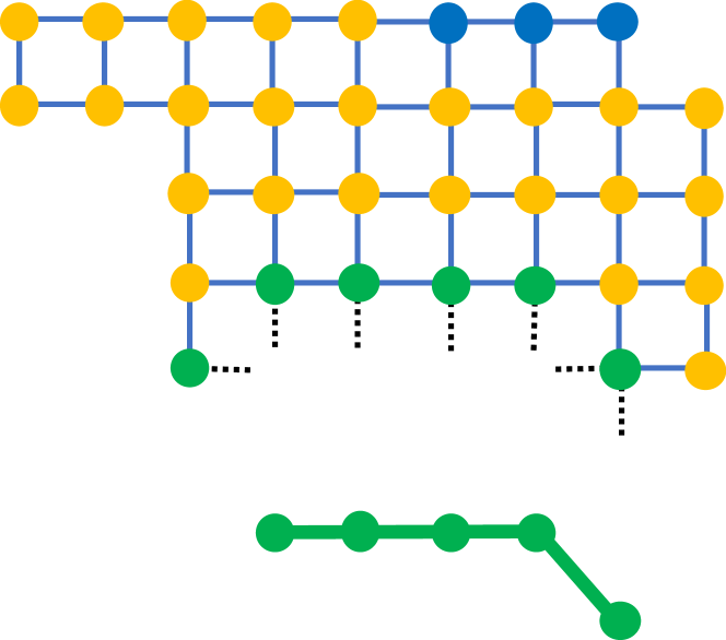
Figure 7: Illustration of the concept of self-energy for the system shown in Fig. 6. After integrating out the lower part of Fig. 6, there remains the upper part of the system (upper panel) connected to a self-energy term (lower panel) to be added to the Hamiltonian.

An alternative way for using the Dyson equation is to “integrate out” some of the sites present in the system, which we now illustrate. To this end, we will use an additional structure, namely the fact that the two different parts of Fig. 6 (as separated by the dotted lines) are unconnected before $\mathds{H}_{1}$ connect them. In other words $\mathds{G}^{\text{CC}}_{0}$ is block diagonal in this upper/lower (denoted as up/lo, respectively) block substructure while $\mathds{H}_{1}$ is purely block off-diagonal:

$$\mathds{G}^{\text{CC}}_{0}=\begin{pmatrix}\mathds{G}_{0}^{\text{up}}&0\\ 0&\mathds{G}_{0}^{\text{lo}}\end{pmatrix}$$ (128)

$$\mathds{H}_{1}=\begin{pmatrix}0&\mathds{V}^{\dagger}\\ \mathds{V}&0\end{pmatrix}$$ (129)

With this additional structure Eq. (125) takes the form

$$G_{0}^{\text{CC}}=\begin{pmatrix}\left(\mathds{G}_{0}^{\text{up}}\right)^{-1}&-\mathds{V}^{\dagger}\\ -\mathds{V}&\left(\mathds{G}_{0}^{\text{lo}}\right)^{-1}\end{pmatrix}^{-1}.$$ (130)

Using $\left(\mathds{G}_{0}^{\text{up}}\right)^{-1}=E-\mathds{H}_{\text{up}}$ and using the block inverse formula we find

$$\mathds{G}^{\text{up}}=\frac{1}{E-\mathds{H}_{\text{up}}-\Sigma_{\text{lo}}(E)}$$ (131)

where the self-energy $\Sigma_{\text{lo}}(E)$ is given by,

$$\Sigma_{\text{lo}}(E)=\mathds{V}^{\dagger}\mathds{G}_{0}^{\text{lo}}\mathds{V}.$$ (132)

In other words, the lower part has been condensed into a self-energy term within the Hamiltonian of the upper part. In contrast to the Hamiltonian, however, the self-energy is a dense matrix (that connects all the green sites of the lower part together), is non-Hermitian and depends on the energy (schematically shown in Fig. 7). The self-energy approach can be used to “decimate” the sites one after the other until one is left with only the sites of interests [217]. However, one should keep in mind an important point in the definition of the retarded Green’s functions: for infinite systems, the matrix elements of the Green’s functions are smooth functions of the energy. For finite systems they are however essentially the sum of Dirac functions positioned at the eigenenergies of the system, and therefore ill-defined numerically. Hence, the decimation is usually performed starting from a semi-infinite lead. Alternatively, one can calculate the Green’s function slightly away from the real axis but that leads to algorithms that require extrapolation and are not very robust.

Finally, we note that the Dyson equation can be used to recover some of the important equations derived earlier. We consider the case where $\mathds{H}_{1}$ is the part of the Hamiltonian matrix that connects the lead to the scattering region. $\mathds{G}_{0}$ is the Green function of the disconnected scattering region + lead system. Then $\mathds{G}^{\text{up}}_{0}=(E-H_{\text{sr}})^{-1}$, $\mathds{G_{0}^{\text{lo}}}=G_{\text{lead}}$, and $\mathds{V}=VP_{\text{sr}}$. With this, Eq. (130) can be recasted as

$$\begin{pmatrix}E-H_{\text{sr}}&-P_{\text{sr}}^{T}V^{\dagger}\\ -VP_{\text{sr}}&G_{\text{lead}}^{-1}\end{pmatrix}\mathds{G}^{\text{CC}}=1$$ (133)

which we recognize as Eq. (96) before block-matrix inversion. Hence, we see that we can recover the definition of the self-energy without any prior knowledge of the lead modes. In fact, this derivation is even more general since it does not explicitly assume that the lead has translational symmetry.

VI.4 The recursive Green’s function (RGF) algorithm and its extensions

The RGF algorithm plays an important role in quantum transport as one of the first available numerical technique that was developed first in one dimension [158, 278] and then extended to quasi-one dimension [181] for addressing disordered systems and later to ballistic multi-terminal systems [24]. Here we step away from the historical formulations and explain the RGF algorithm in a slightly more general way in terms of the gluing sequence of the preceding section.

Fig. 8 shows a schematic of the recursive Green’s Function algorithm (RGF) for a rectangular sample of width $W$ and length $L$. One first needs to calculate the Green’s function of the translationally invariant semi-infinite electrode. These matrix elements need only be computed for the last slice of sites (the so called surface Green’s function), and can be computed with one of the methods explained in Sec. VI.1.

Once one has the electrode surface Green’s function, RGF simply uses the gluing sequence to iteratively add one slice after the other of the scattering region from left to right. When all slices have been added, finally the right electrode is glued to the system. The overall complexity of RGF scales as $W^{3}L$ as can be seen from the equations of the gluing sequence (one $W\times W$ matrix inversion per slice added). It is therefore very efficient for systems that are close to being one-dimensional $L\gg W$.

The original RGF algorithm has been generalized to different strategies for a parallel implementation [78] and adding slices of different shapes in an optimized way. This can be done using algorithms for analyzing the connectivity graph of the Hamiltonian matrix [307, 189, 197, 167], using minimum slices with just a single site [130] or circular slicing [277]. These more recent algorithms have the advantage of being easy to deploy on multi-terminal systems, arbitrary geometries and lattices but have a scaling similar to RGF. Other approaches take advantage of a structure of the problem, such as some parts of the device being defect free, to speed up the calculation [276]. [193] extends RGF to calculate other quantities than the transmission probability such as the local density of states.

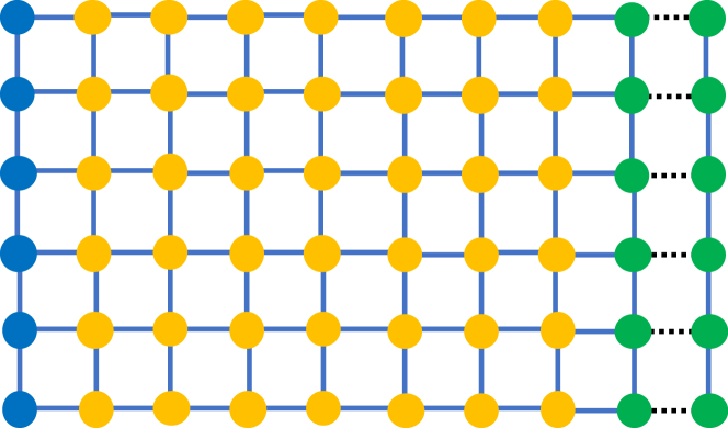
Figure 8: Schematic of one step of the original recursive Green’s Function (RGF) algorithm. the gluing sequence is used iteratively to add new sites slice by slice. The site coloring is the same as in Fig. 6

For systems whose different dimensions are of similar sizes ($L\approx W$), an efficient way to build the system is to use the nested dissection algorithm [147, 165]. In nested dissection one recursively double the system size by using the gluing sequence according to the schematic of Fig. 9. For a $L\times L$ square system, the computing time reduces to $L^{3}$ which is parametrically faster than the $L^{4}$ of RGF. However, implementing the nested dissection algorithm in a stable way is not easy as it implies gluing blocks that are not connected to the electrodes (hence finite with badly conditioned Green’s functions, see the discussion above). It can thus be beneficial to use one of the existing direct sparse solvers as discussed in Sec. VI.2.

There have been many algorithms related to RGF that all rely on some form of the gluing sequence. Those include the modular Green’s function algorithm [241, 240], the (parallel) patchwork algorithm [63] or matching methods [31] that glue together various precalculated subparts of the system. Other applications include multiscale modeling [52] where a central part of the system is described accurately within DFT while the periphery is modeled by a parametrized tight-binding model.

A very closely related class of algorithm uses “decimation” to integrate out sites that are not of direct interest. The sites integrated out appear through self-energy terms. Despite being apparently different, these algorithms are very close to RGF kind of algorithms. Early algorithms include [103, 217].

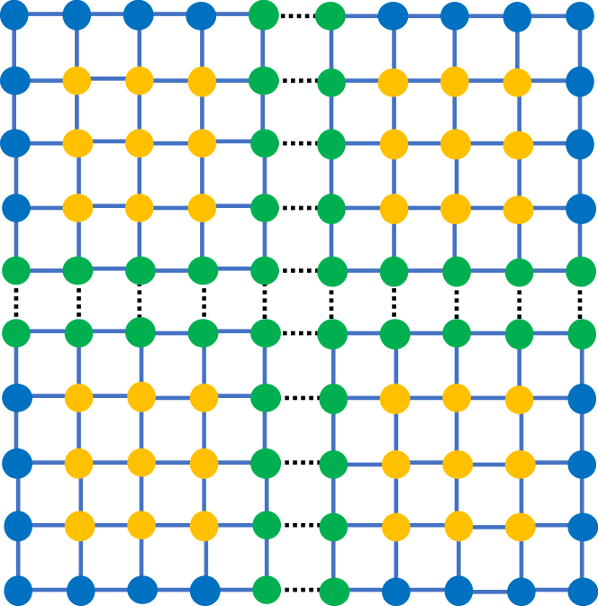
Figure 9: Schematic of one step of the nested dissection algorithm. The gluing sequence is used to recursively double the size of a $L\times L$ square system to a $2L\times 2L$ system. The site coloring is the same as in Fig. 6

VI.5 Other approaches beyond this review, discussion.

In the early days of RGF, another competing algorithm was written in terms of the transfer matrix that relates the wave-function in one layer to the next [285]. The transfer matrix algorithm requires to be stabilized against accumulation of errors as it does not naturally preserve unitarity [286]. It has been mostly abandoned in favor of RGF.

The RGF class of algorithms have a computational effort that scales as $L^{3d-2}$. These algorithms are very efficient in one dimension of for very elongated systems. For systems where all dimensions have similar sizes, approached based on nested dissection are parametrically faster and in practice outperform RGF for $L\geq 100$ [104]. In two dimensions a calculation of a squared system of $10^{6}$ sites takes less than 1 hour on a single core, making 2D calculations easily tractable.

In three dimensions, the situation is more complex since it is difficult to calculate systems large enough for the calculations not to be dominated by finite size effects. An alternating idea to RGF kind of calculations is to use a different starting point: instead of starting from vacuum and adding sites layers by layers, one may start from a pristine material and use Dyson equation to modify a finite number of Hamiltonian matrix elements [208, 256]. This approach allows one to start directly in the thermodynamic limit hence address difficult 2D or 3D systems. In some simple cases, the pristine Green’s function may be obtain analytically through complex contour integration [208, 253, 256]. The method has been generalized by [119] to arbitrary pristine systems by a numerical calculation of the poles and residues of the problem.

When the current is forced to go through a small constriction with very few propagating channel, one may take advantage of this fact to build an effective quasi-1D problem that is much faster to solve [69, 70] even if the original electrodes are fully 3D.

For quantities that are mostly local such as the electronic density, local density of states or the conductivity (as opposed to the full conductance of a device that is essentially global), linear scaling methods such as the Kernel Polynomial Method (KPM) can be very efficient [304]. Linear scaling methods for transport have been recently reviewed in [83].

This review has focused on discrete models. In some specific cases, it is also possible to perform wave-matching directly in the continuum [274, 286, 64] or by treating part of the system (e.g., the leads) directly in the continuum [159].

Last, let us mention two alternative techniques that are slightly different from the mainstream approach. The Complex Absorbing Potential (CAP) technique can be used to bypass solving the lead problem by including a finite part of the lead in the calculation in presence of a smoothly varying complex potential [77]. In the Contact Block Reduction (CBR) approach, one approximates the Green’s function of the isolated scattering region part by selecting only a finite fraction of the eigenstates of the closed system [183].

VII Physical observables in the Landauer-Büttiker approach

So far, we have been concerned solely with one-body quantum mechanics. We now turn to expressing the out-of-equilibrium observables, such as the conductance, in terms of the solution of the quantum mechanical problem, i.e., we now incorporate statistical physics.

Introducing the destruction $c_{n}$ (creation $c^{\dagger}_{n}$) operators on site $n$, we are now considering Hamiltonians in second-quantized form,

$${\cal H}=\sum_{nm}\hat{H}_{nm}c^{\dagger}_{n}c_{m}.$$ (134)

where the matrices $\hat{H}$ correspond to the various infinite matrices of the one-body problem.

VII.1 Many-body steady states

The solutions of the scattering problem $\hat{\psi}(E)$ computed in Sec. III.3 together with the bound states from Sec. III.5 form a complete basis of single-particle wave functions of the Hamiltonian (46).

Because we focus on time-independent quantum transport, we limit our consideration to steady many-body states, where each of the single particle states has a specific occupation number $f_{\alpha E}$. Requiring additionally that the fermion occupation numbers are uncorrelated, we obtain the general form of the density matrix of such states

$$\rho =\prod_{\alpha E}\left([1-f_{\alpha}(E)](1-\Psi_{\alpha E}^{\dagger}\Psi_{\alpha E})+f_{\alpha}(E)\Psi_{\alpha E}^{\dagger}\Psi_{\alpha E}\right),$$ (135)

$$\Psi_{\alpha E} =\sum_{n}\hat{\psi}_{\alpha E,n}c_{n}.$$ (136)

The single particle density matrix for such a state is

$$\langle c^{\dagger}_{n}c_{m}\rangle=\sum_{\alpha}\int\frac{dE}{2\pi}\hat{\psi}_{\alpha E,n}^{*}\hat{\psi}_{\alpha E,m}f_{\alpha}(E)$$ (137)

where we remember that the density of state of the one dimensional channels has been already incorporated (up to the factor $2\pi$) in the normalization of the wave function. Indeed, we normalize the states to carry unit current and in one dimension the velocity $(1/\hbar)dE/dk$ is the inverse of the density of state. When the sites $n,m$ belong to the scattering region, we arrive at

$$\langle c^{\dagger}_{n}c_{m}\rangle=\sum_{\alpha}\int\frac{dE}{2\pi}(\Psi_{\text{sr}}^{*})_{n\alpha}(\Psi_{\text{sr}})_{m\alpha}f_{\alpha}(E)$$ (138)

which is expressed in terms of quantities that we learned to calculate. We narrow our scope further and consider one particularly important class of steady states where each of the leads has fixed chemical potential voltage $\mu_{a}$ and temperature $\Theta_{a}$. Then the modes $\hat{\psi}_{\alpha E}$ incoming from the lead $a$ have an occupation number given by the Fermi distribution of that lead

$$f_{a}(E)=\frac{1}{e^{\beta_{a}(E-\mu_{a})}+1},$$ (139)

with $\beta=1/k_{b}\Theta$. It is worth noting that, although such a steady state is not a thermal state (the different leads can have different temperatures and/or chemical potentials), Eq. (135) is the thermal state of the effective nonlocal Hamiltonian $H_{\mathrm{eff}}$,

$$\rho=\frac{1}{Z}e^{-H_{\mathrm{eff}}},\quad H_{\mathrm{eff}}=\sum_{\alpha E}\beta_{a}(E-\mu_{a})\Psi^{\dagger}_{\alpha E}\Psi_{\alpha E}.$$ (140)

This form makes it explicit that the Wick theorem is applicable to this density matrix. ($Z$ is the partition function that ensures normalization).

VII.2 Landauer formula and its generalizations

All the observable quantities follow from the solution of the scattering problem, namely from the quantities $\Phi$, $\Lambda$, $S_{\mathrm{tp}}$, $\Psi_{\text{sr}}$. The most important object is the scattering matrix $S=S_{\mathrm{pp}}$ between propagating modes. We use the abbreviated notation $S_{\alpha\beta}=[S_{\mathrm{pp}}]_{\alpha\beta}$ for the corresponding matrix elements between channel $\alpha$ and $\beta$. Below we review the formulae used for the most common observables calculated in quantum transport.

VII.2.1 Electric current and conductance

In analogy to the derivation of Eq. (13), the out-of-equilibrium current that flows through lead $a$ reads,

$$I_{a}=\frac{e}{h}\sum_{b}\int dE\sum_{\alpha\in a,\beta\in b}\left|S_{\alpha,\beta}\right|^{2}\left[f_{b}(E)-f_{a}(E)\right]\,.$$ (141)

Here, we use the convention that current $I_{a}>0$ means current flowing towards the scattering region and the electron charge is $-e$ with $e>0$. Using the unitarity of the scattering matrix $S$, this expression can be rewritten as

$$I_{a}=\frac{e}{h}\sum_{b}\int dE\,g_{ab}(E)\,f_{b}(E)\,,$$ (142)

where $g_{ab}(E)$ is defined as

$$g_{ab}(E)=\sum_{\alpha\in a,\beta\in b}(|S_{\alpha,\beta}|^{2}-\delta_{\alpha,\beta}\delta_{a,b})\,.$$ (143)

For $a\neq b$, $g_{ab}(E)$ is the total transmission from lead $b$ to lead $a$. $g_{aa}(E)$ is negative, with $|g_{aa}(E)|$ equal to the total transmission from lead $a$ to all other leads $b$.

While Eq. (142) is now very well established and has been validated in particular by the observation of the quantization of conductance in quantum point contacts, several other formula were initially proposed [51].

When all the leads have equal temperatures and the voltage applied $V_{a}$ are small $\mu_{a}=E_{F}-eV_{a}$, we get in linear response,

$$I_{a}=\sum_{b}\mathcal{G}_{ab}V_{b}\,,$$ (144)

with the conductance matrix defined as,

$$\mathcal{G}_{ab}=\frac{e^{2}}{h}\int\ dEg_{ab}(E)\ \frac{\partial f}{\partial E}(E)\,.$$ (145)

At zero temperature, this expression further reduces to what is known as the multi-terminal Landauer formula [49].

$$\mathcal{G}_{ab}=-\frac{e^{2}}{h}g_{ab}(E_{F})\,.$$ (146)

The $N_{\mathrm{leads}}\times N_{\mathrm{leads}}$ conductance matrix $\mathcal{G}_{ab}$ satisfies current conservation, $\sum_{a}\mathcal{G}_{ab}=0$. Additionally gauge invariance requires that adding a constant to all voltages does not change currents, therefore $\sum_{b}\mathcal{G}_{ab}=0$. In other words the vector $\mathbb{1}=(1,1,\ldots,1)^{T}$ is both a left and a right eigenvector of the $\mathcal{G}_{ab}$ matrix with eigenvalue zero. Note that both relations are due to the unitarity of the scattering matrix $S$.

A commonly occurring measurement technique of multiterminal samples is to send a current between two electrodes, while measuring all the possible voltage differences. In particular, the four terminal resistance is

$$R_{ab,cd}=\frac{V_{a}-V_{b}}{I}\,,$$ (147)

with $V_{a}$ and $V_{b}$ corresponding to $I_{c}=-I_{d}=I$, and all the other currents equal to 0. The four terminal resistance can correspond to longitudinal or Hall resistance depending on the measurement configuration. For $c=a$ and $d=b$ it corresponds to a two-terminal resistance. Because the conductance matrix has a zero eigenvalue, straightforward inversion of Eq. (144) to calculate $R_{ab,cd}$ is impossible. A possible workaround is eliminating a single row (the corresponding current can be calculated at a later stage using current conservation) and a column (this is equivalent to fixing the voltage on the corresponding terminal to 0) of the conductance matrix and invert the truncated conductance matrix. An alternative solution is to use our knowledge of the zero eigenvector of $\mathcal{G}$ to construct the resistance matrix as a pseudoinverse. Introducing the projector $\mathbb{P}=\mathbb{1}\mathbb{1}^{T}/N_{\mathrm{leads}}$ onto the kernel of $\mathcal{G}$, one can simply shift the matrix $\mathcal{G}$ by an arbitrary constant $a\neq 0$ times $\mathbb{P}$ to make it invertible. This allows one to define the voltage $V$ as,

$$V=(\mathcal{G}-a\mathbb{P})^{-1}I\,.$$ (148)

Indeed, when the vector $I$ satisfies current conservation (i.e., $\mathbb{P}I=0$), Eq.(148) implies that the average of $V$ vanishes (i.e., $\mathbb{P}V=0$ since, i.e., $\mathbb{P}\mathcal{G}=0$) and it follows that $V$ satisfies $I=\mathcal{G}V$.

Note that the conductance matrix from Eq. (144) only takes into account the device described by the scattering region. In an experiment, the device will be connected to electric lines that have a resistance that can be comparable to the one of the device. In that situation, reconstructing the conductance matrix needs additional care as one needs to embed it inside a classical electric circuit. This can be further complicated if nonlinear effects start to play a role.

VII.2.2 Conductance in normal/superconductor hybrids

If one grounded superconducting electrode is present in the system, the conductance can still be described with the scattering formalism using the Bogoliubov-De Gennes wave function (see also Sec. IX.5). In this case, charges may enter the superconductor in Cooper pairs resulting in Andreev reflection a process when an incoming electron $e$ converts into an outgoing hole $h$ in the same lead via Andreev reflection, or in a different lead via crossed Andreev reflection.

The current in a normal lead $a$ is then given as [152]

$$I_{a}=\frac{e}{h}\sum_{b}\int dEg_{ab}(E)\left[f_{b}(E)-f_{\text{S}}(E)\right]\,,$$ (149)

where the summation is over all normal leads $b$, $f_{\text{S}}(E)$ the Fermi-Dirac distribution function of the grounded superconductor, energy $E$ is defined with respect to the Fermi level of the superconductor, and

$$g_{ab}(E)=\sum_{\alpha\in a,\beta\in b}|S_{\alpha e,\beta e}|^{2}-|S_{\alpha h,\beta e}|^{2}-\delta_{\alpha e,\beta e}\delta_{a,b}\,.$$ (150)

This conductance matrix is only valid for the normal leads, and alone does not exhibit current conservation. The reason for this is the presence of the superconductor, that not only allows current in the quasi-particle continuum but also in the Cooper pair condensate.

In typical experiments, bias voltages are on the order of the superconducting gap. Since the conductance of a normal/superconductor hybrid changes drastically over this energy scale [36], conductance is usually not considered in linear response in this case. Instead, it is obtained by taking the derivative of Eq. (149) with respect to the voltage $V_{b}$. In the limit of temperatures much lower than the superconducting gap, the Fermi-Dirac distribution is well-approximated by a step function and we find

$$\frac{dI_{a}}{dV_{b}}=-\frac{e^{2}}{h}g_{ab}(-eV_{b})\,.$$ (151)

Cases with more than one superconducting lead are beyond the scope of this review. Then, currents can flow in equilibrium (DC Josephson effect) and voltage differences can lead to time-dependence (AC Josephson effect, multiple Andreev reflection [22]).

VII.2.3 Thermoelectric effects

Equation (142) can also be used to calculate Seebeck effects by introducing temperature gradients [261]. In the limit of small gradients, $k_{B}\Theta_{a}=k_{B}\Theta_{\mathrm{av}}+k_{B}\delta\Theta_{a}$, we find

$$I_{a}=\sum_{b}\mathcal{G}^{S}_{ab}\,\delta\Theta_{b}\,,$$ (152)

with the Seebeck conductance matrix defined as

$$\mathcal{G}^{S}_{ab}=\frac{e}{h\Theta_{\mathrm{av}}}g_{ab}^{(1)}\,,$$ (153)

where we have introduced

$$g_{ab}^{(n)}=\int dE\ g_{ab}(E)\left(-\frac{\partial f}{\partial E}\right)(E)(E-E_{F})^{n}\,.$$ (154)

At low temperatures $\Theta_{\mathrm{av}}$, the expression simplifies after a Bohr-Sommerfeld expansion to

$$\mathcal{G}^{S}_{ab}=\frac{e\pi^{2}k_{B}^{2}\Theta_{\mathrm{av}}}{3h}\frac{\partial g_{ab}}{\partial E}(E_{F})\,.$$ (155)

In analogy with the charge current, one can further introduce the heat current as the energy flowing in the lead, counted from the chemical potential,

$$I_{a}^{H}=-\frac{1}{h}\sum_{b}\int dE\,g_{ab}(E)(E-\mu_{a})\left[f_{b}(E)-f_{a}(E)\right]\,.$$ (156)

Here we use sign conventions such that $I_{a}^{H}>0$ means heat flowing towards the scattering region. In the limit of small bias voltages, one gets the Peltier effect

$$I_{a}^{H}=\sum_{b}\mathcal{G}^{P}_{ab}\,\,V_{b}$$ (157)

with the Peltier conductance matrix defined as

$$\mathcal{G}^{P}_{ab}=\frac{e}{h}g_{ab}^{(1)}=\Theta_{\mathrm{av}}\mathcal{G}^{S}_{ab}\,.$$ (158)

The direct correspondence with the Seebeck effect is a consequence of the thermodynamic Onsager relations. Last, in the limit of small temperature gradients, we get

$$I_{a}^{H}=\sum_{b}\mathcal{G}^{H}_{ab}\,\delta\Theta_{b}\,,$$ (159)

with the Heat conductance matrix defined as,

$$\mathcal{G}^{H}_{ab}=\frac{1}{h\Theta_{\mathrm{av}}}g_{ab}^{(2)}\,.$$ (160)

In the limit of small temperature, the Heat conductance simplifies into

$$\mathcal{G}^{H}_{ab}=-\frac{\pi^{2}k_{B}^{2}\Theta_{\mathrm{av}}}{3h}g_{ab}(E_{F})\,.$$ (161)

We note that in this limit, we recover

$$\frac{\mathcal{G}^{H}_{ab}}{\Theta_{\mathrm{av}}\mathcal{G}_{ab}}=\frac{\pi^{2}k_{B}^{2}}{3e^{2}}\,,$$ (162)

the (mesoscopic version of the) Wiedemann-Franz law.

VII.2.4 Spin currents

A Landauer formula can also be derived for spin currents. It can be used to calculate, e.g., the spin torque exerted on a magnetic layer by an injected current [294, 37]. The definition of the spin current, which provides an explicit link between spin current and spin torque, is obtained from the continuity equation of the current [293]. Introducing the vector of Pauli matrices $\vec{\sigma}=(\sigma_{x},\sigma_{y},\sigma_{z})^{T}$, the spin current $\vec{I}$ flowing through a surface $\Sigma$ takes the form $\propto\int_{\vec{r}\in\Sigma}d\vec{r}\ \mathrm{Im}\ \sum_{\eta\eta^{\prime}}\Psi_{\eta}(\vec{r})\vec{\sigma}_{\eta\eta^{\prime}}\vec{\nabla}\Psi_{\eta^{\prime}}(\vec{r})$ where $\Psi_{\eta}(\vec{r})$ is the wave function for the spin component $\eta$. In other words, the spin current is formally equivalent to the charge current with an addition of Pauli matrices in its definition. In the limit of zero temperature and small bias voltages, the spin current takes the form

$$\vec{I}_{a}=\sum_{b}\vec{\mathcal{G}}_{ab}\,V_{b}\,,$$ (163)

where the spin conductance matrix $\vec{\mathcal{G}}_{ab}$ between non-magnetic leads $a$ and $b$ takes the form

$$\vec{\mathcal{G}}_{ab}=\frac{e}{4\pi}\sum_{\eta\eta^{\prime}\eta^{\prime\prime}}\sum_{\alpha\in a,\beta\in b}\vec{\sigma}_{\eta\eta^{\prime}}S_{\alpha\eta^{\prime},\beta\eta^{\prime\prime}}(E_{F})S_{\alpha\eta,\beta\eta^{\prime\prime}}^{*}(E_{F})\,.$$ (164)

Here, the scattering matrix is defined for states with a well-defined spin component $\eta$, i.e., this expression is only applicable to leads where spin is a conserved quantity. Spin currents, being transfer of spin quanta $\hbar$ per unit time, have the dimensions of energy.

Note that in contrast to charge current, there is no conservation of spin current in a magnetic system. Hence, it may be needed to calculate the spin current inside the system as well as in the lead. This can be done using Eq. (138). There is also no “Gauge invariance” so that spin current can flow in the system at equilibrium. In the absence of spin-orbit coupling, such a spin current can be identified with magnetic exchange interaction [43, 293].

VII.2.5 Injectivities and Emissivities

Two secondary concepts of the Landauer-Büttiker formalism are the emissivity and the injectivity [47, 50]. The injectivity $\partial\langle c_{n}^{\dagger}c_{n}\rangle/\partial\mu_{a}$ expresses how much the electronic density $\langle c_{n}^{\dagger}c_{n}\rangle$ varies when one raises the chemical potential $\mu_{a}$ of lead $a$. The emissivity $\partial I_{a}/\partial(H_{\text{sr}})_{nn}$ is the variation of current $I_{a}$ upon a change of electric potential $(H_{\text{sr}})_{nn}$. These two concepts arise naturally when one extends quantum transport to AC regimes or non-linear regimes to introduce a minimum treatment of the effect of electron-electron interactions, see the discussion around Eq. (230).

The injectivity arises naturally in the formalism and reads at zero temperature,

$$\frac{\partial\langle c_{n}^{\dagger}c_{n}\rangle}{\partial\mu_{a}}=\frac{1}{2\pi}\sum_{\alpha\in a}|\Psi_{\text{sr}}(\mu_{\alpha})|_{n\alpha}^{2}\,,$$ (165)

where the scattering wave function $\Psi_{\text{sr}}$ is calculated at $E=\mu_{\alpha}$. Other generalizations can be obtained from Eq. (138) in a straightforward manner.

To obtain the emissivity, one differentiates Eq. (50) and arrives at the following linear system,

$$\begin{pmatrix}H_{\text{sr}}-E&P_{\text{sr}}^{T}V^{\dagger}\Phi_{\mathrm{t+}}\Lambda_{\mathrm{t+}}\\ VP_{\text{sr}}&-V\Phi_{\mathrm{t+}}\end{pmatrix}\begin{pmatrix}\frac{\partial\Psi_{\text{sr}}}{\partial(H_{\text{sr}})_{nm}}\\ \frac{\partial S_{\mathrm{tp}}}{\partial(H_{\text{sr}})_{nm}}\end{pmatrix}=\begin{pmatrix}-\Xi\Psi_{\text{sr}}\\ 0\end{pmatrix}$$ (166)

that must be solved numerically. Here, the matrix $\Xi$ is defined as $\Xi_{ij}=\delta_{in}\delta_{jm}$. Equation (166) can be used to implement automatic differentiation schemes in quantum transport calculations. Eq. (166) has the same structure as Eq. (93) from which it follows that the emissivity can also be obtained from the knowledge of the Green function,

$$\frac{\partial\Psi_{\text{sr}}}{\partial(H_{\text{sr}})_{nm}}=G_{\text{sr}}\Xi\Psi_{\text{sr}}$$ (167)

$$\frac{\partial S_{\mathrm{tp}}}{\partial(H_{\text{sr}})_{nm}}=G_{\mathrm{t+}}\Xi\Psi_{\text{sr}}$$ (168)

VII.3 Quantum noise

The observables defined in the preceding sections are all one-body observables, i.e., mean observables. Another class of important observables are the quantum fluctuations around the mean and in particular the quantum fluctuation of the current [35]. The general expression of the noise correlation $\bar{S}_{ab}(\omega)$ between lead $a$ and $b$ (noise power when $a=b$) at finite frequency $\omega$ reads,

$$\begin{split}\bar{S}_{ab}&(\omega)=\frac{e^{2}}{h}\sum_{c,d}\sum_{\gamma\in c,\delta\in d}\int dE\\ &A^{cd}_{\gamma\delta}(a,E,E+\hbar\omega)A^{dc}_{\delta\gamma}(b,E+\hbar\omega,E)\\ &\{f_{c}(E)[1-f_{d}(E+\hbar\omega)]+f_{d}(E+\hbar\omega)[1-f_{c}(E)]\}\end{split}$$ (169)

where $A^{cd}_{\gamma\delta}(a,E,E^{\prime})$ is defined in terms of the scattering matrix as,

$$A^{cd}_{\gamma\delta}(a,E,E^{\prime})=\delta_{ac}\delta_{ad}\delta_{\gamma\delta}-\sum_{\alpha\in a}S_{\alpha\gamma}^{*}(E)S_{\alpha\delta}(E^{\prime})$$ (170)

Eq. (169) has a number of simplified forms, notably at zero frequency, small bias, zero temperatures, etc. We refer to [35] for a comprehensive review. See also the next section for a simple route for deriving such formula.

VIII Physical observables: the Non-equilibrium Green’s function approach

In this section, we take an alternative, yet equivalent, route compared to the one in the preceding section to calculate out-of-equilibrium physical observables such as the electric conductance from the solution of the quantum mechanical problem. While, in the preceding section, the latter was expressed in terms of the scattering matrix and scattering states, here quantum propagation is encoded in the retarded Green’s function.

The connection from the retarded Green’s function to the physical observable is done through the so-called Keldysh formalism [133]. As we do not consider electron-electron interactions, but simpler quadratic Hamiltonians, the Keldysh formalism considerably simplifies into what is often known as NEGF (Non Equilibrium Green Function’s) formalism [55, 191]. NEGF is mathematically equivalent to the Landauer-Büttiker approach. It is perhaps less intuitive but has the advantage that once a few basic equations have been established, everything follows from straightforward algebra.

VIII.1 Keldysh formalism in a nutshell

In this subsection, we summarize the main definitions and results of the Keldysh formalism that will be needed. We refer the reader to textbooks such as [233, 266] for the derivation of the results that we state here without proofs.

The Keldysh formalism introduces two independent Green’s functions, the “lesser” ($<$) and “greater” ($>$) Green’s functions

$$\hat{G}^{<}_{nm}(\tau) = i\langle c^{\dagger}_{m}e^{i{\cal H}\tau}c_{n}e^{-i{\cal H}\tau}\rangle,$$ (171)

$$\hat{G}^{>}_{nm}(\tau) = -i\langle e^{i{\cal H}\tau}c_{n}e^{-i{\cal H}\tau}c^{\dagger}_{m}\rangle.$$ (172)

These Green’s functions are very convenient since at $\tau=0$ they correspond directly to the observables (e.g., density or current) of interest. From these two Green’s functions, one may construct the “time-ordered” ($T$) , “anti-time ordered” ($\bar{T}$), “retarded” ($R$) and “advanced” ($A$) Green’s functions as,

$$\hat{G}^{T}_{nm}(\tau) = \theta(\tau)\hat{G}^{>}_{nm}(\tau)+\theta(-\tau)\hat{G}^{<}_{nm}(\tau),$$ (173)

$$\hat{G}^{\bar{T}}_{nm}(\tau) = \theta(\tau)\hat{G}^{<}_{nm}(\tau)+\theta(-\tau)\hat{G}^{>}_{nm}(\tau),$$ (174)

$$\hat{G}^{R}_{nm}(\tau) = \theta(\tau)\hat{G}^{>}_{nm}(\tau)-\theta(\tau)\hat{G}^{<}_{nm}(\tau),$$ (175)

$$\hat{G}^{A}_{nm}(\tau) = \theta(-\tau)\hat{G}^{<}_{nm}(\tau)-\theta(-\tau)\hat{G}^{>}_{nm}(\tau).$$ (176)

Note that, in the preceding sections, we encountered only one type of Green’s function, the retarded Green’s function, and the subscript $R$ has been omitted. These Green’s functions are linearly dependent. Below, we will focus on the Green’s functions $\hat{G}^{<}$, $\hat{G}^{R}$ and $\hat{G}^{A}$ using the fact that $\hat{G}^{<}=\hat{G}^{T}-\hat{G}^{R}=\hat{G}^{\bar{T}}+\hat{G}^{A}$ as can be proven trivially from the above definitions.

In this review, we only consider many-body Hamiltonians ${\cal H}$ restricted to be quadratic in the destruction $c_{n}$ and creation $c^{\dagger}_{n}$ operators on site $n$,

$${\cal H}=\sum_{nm}\hat{H}_{nm}c^{\dagger}_{n}c_{m}.$$ (177)

The equivalence between the definition of the retarded Green’s function used in the preceding sections and the one in Eq. (175) is not entirely trivial and indeed valid only for quadratic Hamiltonians. In the following, we make use of this simplification.

In the Keldysh formalism, these Green’s functions naturally appear in the form of a $2\times 2$ matrix associated with the so-called Keldysh contour,

$$\mathbf{\hat{G}}_{nm}(\tau)=\begin{pmatrix}\hat{G}^{T}_{nm}(\tau)&\hat{G}^{<}_{nm}(\tau)\\ \hat{G}^{>}_{nm}(\tau)&\hat{G}^{\bar{T}}_{nm}(\tau)\end{pmatrix}.$$ (178)

Since this review is concerned with d.c. quantum transport (i.e., time-independent Hamiltonians), we’ll work chiefly in energy representation,

$$\mathbf{\hat{G}}_{nm}(E)=\int d\tau\mathbf{\hat{G}}_{nm}(\tau)e^{iE\tau}.$$ (179)

Now that we have defined the mathematical objects of interest, we can state the very few results from non-equilibrium many-body theory that will be needed to establish the basic equations of quantum transport. The equations of motion read

$$\sum_{p}\begin{pmatrix}E\delta_{mp}-\hat{H}_{mp}&0\\ 0&E\delta_{mp}-\hat{H}_{mp}\end{pmatrix}\mathbf{\hat{G}}_{pn}(E)=\begin{pmatrix}\delta_{mn}&0\\ 0&\delta_{mn}\end{pmatrix},$$ (180)

or in compact notations,

$$\begin{pmatrix}E-\hat{H}&0\\ 0&E-\hat{H}\end{pmatrix}\mathbf{\hat{G}}(E)=\begin{pmatrix}1&0\\ 0&1\end{pmatrix}.$$ (181)

Splitting the Hamiltonian matrix $\hat{H}$ into an “unperturbed” matrix $\hat{H}_{0}$ and a “perturbation” $\hat{W}$,

$$\hat{H}=\hat{H}_{0}+\hat{W},$$ (182)

and denoting $\mathbf{\hat{G}}_{0}(E)$ the Green’s function associated with $\hat{H}_{0}$, one can write a form of Dyson equation [233, 266] as

$$\mathbf{\hat{G}}(E)=\mathbf{\hat{G}}_{0}(E)+\mathbf{\hat{G}}_{0}(E)\begin{pmatrix}\hat{W}&0\\ 0&-\hat{W}\end{pmatrix}\mathbf{\hat{G}}(E),$$ (183)

and also

$$\mathbf{\hat{G}}(E)=\mathbf{\hat{G}}_{0}(E)+\mathbf{\hat{G}}(E)\begin{pmatrix}\hat{W}&0\\ 0&-\hat{W}\end{pmatrix}\mathbf{\hat{G}}_{0}(E).$$ (184)

Note that the partition of $\hat{H}$ into $\hat{H}_{0}$ and $\hat{W}$ is arbitrary, although in what follows the $\hat{W}$ matrix will contain the matrix elements that connect the leads to the scattering region and $\hat{H}_{0}$ the rest of the Hamiltonian. Identifying the different components of the $2\times 2$ Dyson equation Eq. (183), one may write

$$\hat{G}^{R} = \hat{G}^{R}_{0}+\hat{G}^{R}_{0}\hat{W}\hat{G}^{R},$$ (185)

$$\hat{G}^{A} = \hat{G}^{A}_{0}+\hat{G}^{A}_{0}\hat{W}\hat{G}^{A},$$ (186)

$$\hat{G}^{<} = \hat{G}^{<}_{0}+\hat{G}^{R}_{0}\hat{W}\hat{G}^{<}+\hat{G}^{<}_{0}\hat{W}\hat{G}^{A}.$$ (187)

The first equation (or equivalently the second one) encodes the quantum mechanics and forms a close set of equations for the retarded Green’s function alone. The third equation encodes the statistical physics. Similarly, Eq. (184) leads to

$$\hat{G}^{R} = \hat{G}^{R}_{0}+\hat{G}^{R}\hat{W}\hat{G}^{R}_{0},$$ (188)

$$\hat{G}^{A} = \hat{G}^{A}_{0}+\hat{G}^{A}\hat{W}\hat{G}^{A}_{0},$$ (189)

$$\hat{G}^{<} = \hat{G}^{<}_{0}+\hat{G}^{R}\hat{W}\hat{G}^{<}_{0}+\hat{G}^{<}\hat{W}\hat{G}^{A}_{0}.$$ (190)

For a system at thermal equilibrium, one has

$$\hat{G}^{<}(E)=-f(E)\left[\hat{G}^{R}(E)-\hat{G}^{A}(E)\right],$$ (191)

which completes the basic formalism that we shall need in this section.

VIII.2 Main NEGF equation

Within the NEGF formalism, computing out-of-equilibrium amounts to performing two tasks. First one computes the retarded Green’s function (i.e., solve the quantum mechanical problem) using, e.g., any algorithm from Sec. VI . Second, one must compute the lesser Green’s function (i.e., the observables). In this subsection, we derive the main result of NEGF that relates the lesser Green’s function to the retarded one in the context of quantum transport. The derivation is a generalization of the original work by Caroli et al. [55]. These results have later been generalized and popularized by Wingreen and Meir [191].

We start by splitting and applying the Dyson equation to $\hat{H}_{\text{sys}}$. The perturbation $\hat{W}$ contains the matrix elements that connect the leads to the scattering region. $\hat{H}_{0}$ contains the Hamiltonian of the disconnected elements of the system: the semi-infinite leads and the isolated scattering region. Let us write Dyson equation in block form where the block index indicates the lead ($a=1,2,\dots$) or the scattering region ($0$). By construction, the disconnected Green’s functions $(\hat{G}_{0})_{kl}=\delta_{kl}(\hat{G}_{0})_{l}$ are diagonal with respect to the block index. Eq. (187) for the scattering region block ${G}^{<}_{\text{sr}}=\hat{G}^{<}_{00}$ reads

$$\hat{G}^{<}_{\text{sr}}=(\hat{G}^{<}_{0})_{0}+(\hat{G}^{R}_{0})_{0}\hat{W}_{0a}\hat{G}^{<}_{a0}+(\hat{G}^{<}_{0})_{0}\hat{W}_{0a}\hat{G}^{A}_{a0},$$ (192)

with an implicit summation over leads $a>0$. Note that in the rest of this section we have absorbed the projection matrices $P_{\text{sr}}$ into $\hat{W}$, such that, e.g., $\hat{W}_{a0}=V_{a}P_{\text{sr}}$, where $V_{a}$ is the hopping matrix of lead $a$. Multiplying Eq. (192) on the left by $E+i\eta-H_{\text{sr}}$ and using $[E-H_{\text{sr}}](\hat{G}^{<}_{0})_{0}=0$ and $[E-H_{\text{sr}}](\hat{G}^{R}_{0})_{0}=1$ we obtain

$$\left[E-H_{\text{sr}}\right]{G}^{<}_{\text{sr}}=\hat{W}_{0a}\hat{G}^{<}_{a0}.$$ (193)

To close the above equation, we write Eq. (187) and (190) for the $a0$ and $0a$ blocks respectively,

$$\hat{G}^{<}_{a0}=(\hat{G}^{R}_{0})_{a}\hat{W}_{a0}{G}^{<}_{\text{sr}}+(\hat{G}^{<}_{0})_{a}\hat{W}_{a0}{G}^{A}_{\text{sr}},$$ (194)

$$\hat{G}^{<}_{0a}={G}^{R}_{\text{sr}}\hat{W}_{0a}(\hat{G}^{<}_{0})_{a}+{G}^{<}_{\text{sr}}\hat{W}_{0a}(\hat{G}^{A}_{0})_{a}.$$ (195)

Inserting Eq. (194) into (193), we arrive at

$$\left[E-H_{\text{sr}}-\hat{W}_{0a}(\hat{G}^{R}_{0})^{a}\hat{W}_{a0}\right]{G}^{<}_{\text{sr}}=\hat{W}_{0a}(\hat{G}^{<}_{0})_{a}\hat{W}_{a0}{G}^{A}_{\text{sr}}.$$ (196)

We recognize Eq. (96) on the left hand side, so that,

$${G}^{<}_{\text{sr}}={G}^{R}_{\text{sr}}\hat{W}_{0a}(\hat{G}^{<}_{0})_{a}\hat{W}_{a0}{G}^{A}_{\text{sr}}.$$ (197)

To conclude, we use Eq. (191) supposing each lead to remain at equilibrium with its Fermi function $f_{a}(E)$. We arrive at the main result of NEGF theory,

$${G}^{<}_{\text{sr}}(E)={G}^{R}_{\text{sr}}(E)\Sigma_{\text{sr}}^{<}(E){G}^{A}_{\text{sr}}(E),$$ (198)

with the lesser self-energy $\Sigma_{\text{sr}}^{<}$ defined as

$$\Sigma_{\text{sr}}^{<}(E)=-\sum_{a}f_{a}(E)\left[\Sigma_{a}^{R}(E)-\Sigma_{a}^{A}(E)\right],$$ (199)

where

$$\Sigma^{R}_{a}=\hat{W}_{0a}(\hat{G}^{R}_{0})_{a}\hat{W}_{a0}$$ (200)

is the partial contribution to the retarded self-energy $\Sigma^{R}(E)=\sum_{a}\Sigma^{R}_{a}$. Since ${G}^{A}_{\text{sr}}=({G}^{R}_{\text{sr}})^{\dagger}$ and ${\Sigma}^{A}_{a}=({\Sigma}^{R}_{a})^{\dagger}$, we can equivalently write Eq. (199) as

$$\Sigma_{\text{sr}}^{<}(E)=i\sum_{a}f_{a}(E)\Gamma_{a}(E)\,,$$ (201)

using definition of the linewidth (106) for lead $a$, $\Gamma_{a}=i(\Sigma^{R}_{a}-\Sigma^{A}_{a})$.

Eq. (198) provides a direct expression of the Lesser Green’s function in terms of the Retarded one and the occupation function in the leads. From there, one can directly calculate physical observables as $\langle c^{\dagger}_{m}c_{n}\rangle=-iG^{<}_{nm}(\tau=0)$ which leads to the one-body density matrix,

$$\langle c^{\dagger}_{m}c_{n}\rangle=-i\int\frac{dE}{2\pi}(G^{<}_{\text{sr}})_{nm}(E),$$ (202)

which generalizes the concept of local density of states to off-diagonal observables and out-of-equilibrium situations.

Inserting Eq. (111) into Eqs. (201) and (198) as well as using Eq. (114) one can relate the lesser Green’s function to the scattering wave-functions; one arrives at [306, 97]

$$G^{<}_{\rm sr}(E)_{nm}=i\sum_{a}f_{a}(E)\sum_{\alpha\in a}\Psi_{\text{sr}}(E)_{n\alpha}\Psi_{\text{sr}}^{*}(E)_{m\alpha}.$$ (203)

At equilibrium, this equation simplifies into $G^{<}_{\rm sr}(E)=i\Psi_{\text{sr}}(E)\Psi_{\text{sr}}^{\dagger}(E)f(E)$ which can be derived straightforwardly using the definition of $G^{<}$ [266].

It is worth noting that there is a subtle point in the derivation above: the limit $\eta\rightarrow 0$ has to be taken at the end of the calculation, not at the beginning, whenever the energy $E$ matches a bound states of the system, owing to the emergence of (diverging) Dirac functions at these energies. It follows that, strictly speaking, one should add the bound states contributions to Eq. (198) or (203) which only contain contributions from the scattering states. For example, Eq. (203) then reads

$$\begin{split}G^{<}_{\rm sr}(E)_{nm}&=i\sum_{a}f_{a}(E)\sum_{\alpha\in a}\Psi_{\text{sr}}(E)_{n\alpha}\Psi_{\text{sr}}^{*}(E)_{m\alpha}\\ &+i\sum_{j}f_{j}(E)\delta(E-E_{j})\left(\Psi_{\text{sr}}\right)_{nj}\left(\Psi_{\text{sr}}^{*}\right)_{mj},\end{split}$$ (204)

where the index $j$ now labels bound states at energy $E_{j}$ with corresponding wave function $(\Psi_{\text{sr}})_{nj}$. These contributions are usually omitted because (i) they do not contribute to transport properties and (ii) the filling factor $f_{i}(E)$ depends on the history of the system and must be decided based on physics not described within our framework [266]. These bound states may play a role nevertheless in certain situations [229].

At equilibrium, the expression for ${G}^{<}_{\text{sr}}$ can be simplified. To do so, we use relation for the Retarded and Advanced Green’s function obtained by (i) multiplying the equation ${G}^{R}_{\text{sr}}(E-H_{\text{sr}}-\Sigma^{R})=1$ by ${G}^{A}_{\text{sr}}$ on the right, (ii) multiplying its Hermitian conjugate $(E-H_{\text{sr}}-\Sigma^{A}){G}^{A}_{\text{sr}}=1$ by ${G}^{R}_{\text{sr}}$ on the left and (iii) subtracting the second equation from the first. One arrives at

$${G}^{R}_{\text{sr}}[\Sigma^{R}-\Sigma^{A}]{G}^{A}_{\text{sr}}={G}^{R}_{\text{sr}}-{G}^{A}_{\text{sr}}.$$ (205)

Inserting Eq. (205) into Eq. (198), we get

$${G}^{<}_{\text{sr}}=-f(E)[{G}^{R}_{\text{sr}}-{G}^{A}_{\text{sr}}],$$ (206)

recovering Eq. (191). Calculating the number of electrons on one site at equilibrium using Eq. (202), we get back the usual expression in terms of the local density of state:

$$\langle c^{\dagger}_{n}c_{n}\rangle=-\int\frac{dE}{\pi}f(E)\mathrm{Im}(G^{R}_{\text{sr}})_{nn}(E).$$ (207)

VIII.3 Landauer formula within NEGF

Let us now define the current flowing towards the scattering region and establish the Green’s function version of the Landauer formula. Introducing the total number of electrons in the scattering region $\mathcal{Q}_{\text{sr}}(t)=\langle{\cal Q}\rangle$ with ${\cal Q}=\sum_{n\in\text{sr}}c^{\dagger}_{n}c_{n}$, the evolution of ${\cal Q}$ (in Heisenberg representation) $\partial{\cal Q}/\partial t=i[{\cal H},{\cal Q}]$ provides the continuity equation

$$\frac{\partial\mathcal{Q}_{\text{sr}}}{\partial t}=\sum_{a}I_{a}(t)\,.$$ (208)

In steady state, i.e., time-independent current flow $I_{a}(t)=I_{a}$, we find the current $I_{a}$ from lead $a$ towards the scattering region as

$$I_{a}=\frac{e}{h}\int dE\operatorname{Tr}[G^{<}_{a0}\hat{W}_{0a}-\hat{W}_{a0}G^{<}_{0a}].$$ (209)

Using Eq. (194), Eq.(195) and the definitions of the self energies we get

$$I_{a}=\frac{e}{h}\int dE\operatorname{Tr}\left[G^{<}_{\text{sr}}(\Sigma^{R}_{a}-\Sigma^{A}_{a})-(G^{R}_{\text{sr}}-G^{A}_{\text{sr}})\Sigma^{<}_{a}\right].$$ (210)

Further using Eqs. (205) and Eq. (201), we finally arrive at

$$I_{a}=\frac{e}{h}\sum_{b}\int dE\operatorname{Tr}\left[G^{R}_{\text{sr}}\Gamma_{b}G^{A}_{\text{sr}}\Gamma_{a}\right]\left[f_{b}(E)-f_{a}(E)\right].$$ (211)

This equation is often (somewhat abusively) referred to as the Landauer formula. It automatically satisfies two important requirements: the absence of incoming currents at equilibrium (note that there may be persistent currents inside the scattering region), and the global conservation of current $\sum_{a}I_{a}=0$.

To conclude this section, we end with the proof that Eq. (211) is indeed equivalent to the (original) scattering matrix version of the Landauer formula. Inserting Eq. (109) and Eq. (111) in Eq. (211) and using the invariance of the trace under cyclic permutation, we get

$$\begin{split}&\operatorname{Tr}\left[G^{R}_{\text{sr}}\Gamma_{b}G^{A}_{\text{sr}}\Gamma_{a}\right]\\ &=\operatorname{Tr}\left[G^{R}_{\text{sr}}\Gamma_{b}\Phi_{\mathrm{p}-}^{b}\Phi_{\mathrm{p}-}^{\dagger b}\Gamma_{b}G^{A}_{\text{sr}}\Gamma_{a}\Phi_{\mathrm{p}+}^{a}\Phi_{\mathrm{p}+}^{\dagger a}\Gamma_{a}\right]\\ &=\operatorname{Tr}\left[\left(i\Phi_{\mathrm{p}+}^{\dagger a}\Gamma_{a}G^{R}_{\text{sr}}\Gamma_{b}\Phi_{\mathrm{p}-}^{b}\right)\left(-i\Phi_{\mathrm{p}-}^{\dagger b}\Gamma_{b}G^{A}_{\text{sr}}\Gamma_{a}\Phi_{\mathrm{p}+}^{a}\right)\right]\\ &=\operatorname{Tr}\left[S^{ab}(S^{ab})^{\dagger}\right],\end{split}$$ (212)

where the $\Phi_{\mathrm{p}+}^{a(b)}$ matrix is restricted to the modes of lead $a$ ($b$). we have introduced a new object $S^{ab}$,

$$S^{ab}=i\Phi_{\mathrm{p}+}^{\dagger a}\Gamma_{a}G^{R}_{\text{sr}}\Gamma_{b}\Phi_{\mathrm{p}-}^{b}\,.$$ (213)

From the Fisher-Lee relation (116), we can indeed identify

$$S^{ab}=S^{ab}_{\text{p}\text{p}},$$ (214)

i.e., the scattering matrix between lead $a$ and lead $b$, restricted to the propagating channels, concluding our of equivalence between the scattering approach and the NEGF approach. Note that in the sum of Eq. (211) only $b\neq a$ contribute, and hence Eq. (212) is valid only for $a\neq b$, i.e., describes transmission from lead $b$ to $a$.

VIII.4 Higher-order observables

The observables defined in the preceding sections are all one-body observables (except for the quantum noise), i.e., quadratic in the creation/destruction operators. To calculate higher-order observables, one can make use of the fact that, even though the system is out of equilibrium, the density matrix is the exponential of a (highly non-local) quadratic Hamiltonian, see Eq.(140). It follows that Wick theorem applies, allowing expression of, e.g., quartic terms in terms of quadratic ones,

$$\langle c^{\dagger}_{n}(t)c_{m}(t) c^{\dagger}_{p}(t^{\prime})c_{q}(t^{\prime})\rangle=$$

$$\langle c^{\dagger}_{n}(t)c_{m}(t)\rangle \langle c^{\dagger}_{p}(t^{\prime})c_{q}(t^{\prime})\rangle+\langle c^{\dagger}_{n}(t)c_{q}(t^{\prime})\rangle\langle c_{m}(t)c^{\dagger}_{p}(t^{\prime})\rangle,$$

i.e., in terms of sum of products of Lesser and Greater Green’s functions. This approach can be used directly to calculate quantities such as shot noise [96].

The same approach can be used to derive expressions relating higher-order observables to the scattering wavefunction. For this, one uses the following dictionary [97] :

$$[G^{<}(\tau)]_{nm}=i\sum_{\alpha}\int\frac{dE}{2\pi}(\Psi_{\text{sr}})_{n\alpha}(\Psi_{\text{sr}}^{*})_{m\alpha}e^{-iE\tau}f_{\alpha}(E),$$ (216)

and

$$[G^{>}(\tau)]_{nm}=-i\sum_{\alpha}\int\frac{dE}{2\pi}(\Psi_{\text{sr}})_{n\alpha}(\Psi_{\text{sr}}^{*})_{m\alpha}e^{-iE\tau}[1-f_{\alpha}(E)].$$ (217)

Note that likewise, the retarded Green’s function can be expressed as

$$[G^{R}(\tau)]_{nm}=-i\theta(\tau)\sum_{\alpha}\int\frac{dE}{2\pi}(\Psi_{\text{sr}})_{n\alpha}(\Psi_{\text{sr}}^{*})_{m\alpha}e^{-iE\tau}.$$ (218)

IX Selected applications to model systems

We have now completed the technical part of this review where we presented the mathematical formalisms and the associated algorithms used to make actual numerical calculations. We are left to discuss how these techniques are used for real world applications. Numerical quantum transport calculations are by now very common in a wide variety of fields ranging from molecular electronics through spintronics to nanoelectronics. They are applied in the study of devices made of semiconductors, graphene, topological materials, superconductors, and various combinations thereof. We shall not attempt to review all these applications but will confine ourselves to selecting a few examples that we find either important or illustrative. Such a choice is necessarily subjective.

IX.1 A hierarchy of discrete models

c|c[cell-space-limits=8pt] 3-1Optionally

self-consistent [fill=[HTML]98db65]1-1Discretized $k\cdot p$ Hamiltonians

[fill=[HTML]c7db65]1-1Tight-binding models (TBM)

[fill=[HTML]dbc365]1-1Semi-empirical tight-binding models

(SE-TBM)

2-1Self-consistent [fill=[HTML]dba065]1-1First principles tight-binding models

(FP-TBM)

[fill=[HTML]db8165]1-1Density functional theory (DFT)

Table 2: Schematic of the different levels of modeling used in numerical quantum transport, see text.

The first step in this regard is to select the appropriate level of modeling for the Hamiltonian of the scattering region as well as of the (semi-infinite) electrodes and of the system-electrode interface. There exists a hierarchy of discrete Hamiltonians that can be used to describe a system, and physicists must select an appropriate level of modeling, requiring a tradeoff between accuracy and numerical tractability. Fig. IX.1 shows a schematic of this hierarchy. At the bottom are calculations performed entirely within the framework of density functional theory. In the absence of strong electronic correlations, DFT provides an accurate description of the system from first principles and has de facto become the reference approach to the calculation of realistic materials. However, strictly speaking, the Kohn-Sham equations of DFT are valid for the ground state of the system and often need to be corrected to properly account for dynamical properties such as the band gap. Next come the First Principle Tight-Binding Models (FP-TBM) where a DFT calculation is followed by the projection of the corresponding (self-consistent) Hamiltonian onto a set of localized states such as maximally localized Wannier functions. Semi-Empirical Tight-Binding Models (SE-TBM) are also models that are derived from a DFT calculation. However, in contrast to FP-TBM where the model is constructed in a systematic way, the SE-TBM are parametrized and then fitted to properly reproduce the DFT calculations (typically the band structure) and/or experimentally known properties of the material (such as the band gap). The orbitals and terms in the Hamiltonian included in the SE-TBM are typically dictated by symmetry and physics considerations. When the Tight-Binding Model (TBM) is not tightly bound to a first principle calculation, we simply call it a general TBM. These TBM’s can be studied from a purely theoretical perspective or in situations where a simple model is sufficient to account for the physics. These model systems can also come from the discretization of a continuum model such as $\mathbf{k.p}$ model or a simple effective mass model. All these models describe essentially the quantum mechanics of the conducting electrons of the system.

Another important ingredient is the electromagnetic and in particular electrostatic environment in which these electrons propagate. In fact, the electrostatic energy is usually the largest energy of the problem. In first principle calculations, the electrostatic problem is solved self-consistently with the quantum mechanical one. In model systems (general TBM and $\mathbf{k\cdot p}$ models) one often assumes that the electric potential is known and has a simple form.

In this section and the next, we will give a few selected examples to illustrate the use of computational quantum transport. In the remaining part of this section, we focus on “model” systems (the two upper types of models in Fig. IX.1) while the next section will focus on more “realistic” models (the three lower levels in Fig. IX.1).

IX.2 Applications to the two-dimensional electron gas

IX.2.1 The early days: Disordered systems and Anderson localization

An important application of numerics to quantum transport is the study of the effect of static disorder on conductance as well as of the associated Anderson localization phenomena. This is perhaps the historically first application of the techniques described in this review and also one of the most successful ones.

The model is the discretized effective mass Schrödinger equation Eq. (22) in the presence of static disorder. In two dimensions the model reads

$$\Psi_{n+1,m} + \Psi_{n-1,m}+\Psi_{n,m+1}+\Psi_{n,m-1}$$ (219)

$$+ V_{n,m}\Psi_{n,m}=E\Psi_{n,m},$$

where the potential $V_{n,m}$ takes different random values on different sites. Typically, one chooses $V_{n,m}$ randomly with a flat distribution $V_{n,m}\in[-W/2,W/2]$ where the parameter $W$ is the strength of the disorder. In a seminal paper, the “gang of four” [1] had predicted that the conductance $g(W,L)$ (where $L$ is the size of the sample) followed a simple scaling law from which one could predict the insulating or metallic behavior of the sample. The scaling hypothesis, which was supported by theoretical arguments both in the strong and weak disorder regimes, was that the function $\beta\equiv\partial\log g/\partial\log L$ was a function of $g$ only (i.e., $\exists f,\ \beta(L,W)=f[g(W,L)]$ ). One of the most striking conclusions of the scaling theory was that in three dimensions there was a critical value of disorder associated to a metal-insulator transition, but in one and two dimensions the system was always an insulator in the sense that the conductance would become vanishingly small in the $L\rightarrow\infty$ limit.

While the scaling hypothesis was plausible, it was merely a hypothesis. It was put on firm grounds in a series of works combining numerical calculations with finite-size scaling analysis. These calculations were pioneered by [223, 224] who, however, wrongly concluded the existence of a metal-insulator transition in two dimensions. Subsequent more precise numerics [182] could indeed confirm the finite-size scaling hypothesis, as shown in Fig. 10. A large activity followed in the following decade with the study of the effect of various parameters such as spin-orbit coupling, magnetic field, type of disorder, as reviewed in [142].

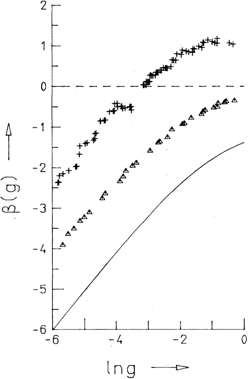
Figure 10: Scaling function $\beta(g)$ computed numerically for a 2D (triangles) and 3D (pluses) tight-binding model, confirming the scaling hypothesis. From [182].

Besides the Anderson localization regime, numerics have also been used to study the quantum corrections to the classical limit in the diffusive regime. An early work in this direction is the study of the universal conductance fluctuations [270]. More recent applications include simulations of diffusive metal-superconductor junctions [186] or disproving of the conjecture of the existence of a two-parameter scaling regime in a system with partially broken time reversal symmetry [255].

IX.2.2 Ballistic systems and Quantum billiards

In the early nineties, the opposite, ballistic regime (no disorder) attracted wide interest in the context of “quantum billiards”. Quantum billiards consist of a high mobility two-dimensional electron gas (typically GaAs/GaAlAs heterostructures) where a billiard is patterned using electrostatic gates deposited on top of the heterostructure. A study of such billiards (also known as quantum dots in the regimes where they are almost closed and charging energy plays an important role) was performed in [122] using the recursive Green’s function algorithm. 4-terminal (X-shaped) and 3-terminal (T-shape) ballistic junctions were studied in [24, 262]. One of the successes of these ballistic calculations was the finding that the statistics of the height of the resonances (in the almost closed regime) matched the Porter-Thomas distribution prediction of random matrix theory [123]. Numerics also clarified weak localization, i.e., the interference contribution to the magneto-conductance [25]. Numerics could in particular clearly distinguish the difference in behavior between the magneto-conductance of integrable and chaotic billiards: a chaotic billiard gives rise to a Lorentzian lineshape for the magnetoconductance, whereas an integrable billiard features a triangular lineshape, as shown in the left panels of Fig. 11. This prediction was soon confirmed experimentally [57], shown in the right panels of Fig. 11. In billiards where there exists a short straight path between the entrance and the exit, the observation of Fano resonances [105] was also well reproduced in numerics [62]. A review of quantum billiards can be found in [7]. Some recent ballistic devices focus on building electronic interferometers analogous to those known in optics [48]. Those systems can also be simulated both with [130] (quantum Hall regime) and without [29] magnetic field.

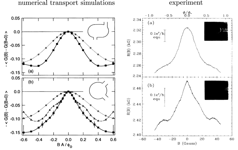
Figure 11: Left: Numerically computed weak localization correction to the conductance for a chaotic stadium billiard (top) and an integrable circular billiard (bottom). Solid lines correspond to specular scattering at the boundary, other lines to a situation with disorder at the boundary. Right: Corresponding experimental data obtained by averaging over 48 billiards defined in a high-quality GaAs electron gas. The lineshape in the chaotic case is Lorentzian and for the integrable billiard triangular, in agreements with simulation. Adapted from [57].

IX.2.3 Scanning gate microscopy

In a scanning gate microscope, one measures how the conductance through a constriction (“a quantum point contact”) is affected by a conducting tip that scans the surface of the heterostructure. Numerical simulations are very handy for these systems as the signal is highly dependent on any residual disorder as well as on the sample geometry. Numerics were shown to correctly capture the experimental observation, at least on a qualitative level [141, 268]. Combined with machine learning techniques, numerical calculations can be used to unveil the underlying disorder potential seen by the electrons [220].

IX.3 Quantum transport in graphene

IX.3.1 Single $p_{z}$-orbital tight-binding model

The discovery of graphene triggered a very large number of numerical studies that is far beyond the scope of the present review [221]. Many of these works use a simple next-nearest neighbor model

$$t\sum_{j=N(i)}\Psi_{j}=E\Psi_{i},$$ (220)

where the site $i$ sits on the hexagonal lattice of graphene and the sum over $j=N(i)$ stands for the three neighbors $j$ of site $i$. The value $t=2.7$ eV is the hopping integral between two neighboring $p_{z}$ orbitals. Recursive Green’s Function algorithms were adapted from the square lattice to the hexagonal case of graphene [162]. They were used very early to check the prediction that the conductivity of pristine graphene at the Dirac point was $4e^{2}/(\pi h)$ while its Fano factor had the same value $1/3$ as in a diffusive wire [283] due to transport through evanescent states in the limit of wide samples. These predictions were later observed experimentally [67]. Recursive Green’s function calculations were also used extensively to study the effect of disorder which makes the conductivity dependent on the disorder strength and correlation length [161] or to assess the regime of validity of, e.g., semi-classical Boltzmann approaches [148].

IX.3.2 Massless Dirac equation

At low energy, pristine graphene is described by 2 independent relativistic Weyl (massless Dirac) equations

$$H_{\mathrm{D}}=v_{F}\begin{pmatrix}0&p_{x}-ip_{y}\\ p_{x}+ip_{y}&0\end{pmatrix}$$ (221)

corresponding to two different valleys K and K’, where the $2\times 2$ structure arises from graphene having two atoms per unit cell. Relativistic equations of this type play an important role in modern condensed matter physics as they arise in a number of topological materials, either in the bulk or for the description of their surface states [303].

Attempts to simulate only one of the two valleys (for instance in order to distinguish between intervalley and intravalley scattering) with any discretization scheme faces the so-called “fermion doubling” problem: in any tight-binding model, Dirac points always come in pairs [273, 200].

This problem can be circumvented by borrowing solutions from the lattice gauge theory [263], such as by evaluating finite differences on a lattice that is displaced symmetrically from the original lattice [282] or by adding a small term which breaks the time-reversal symmetry [116, 107] or $k$-space discretization [27]. See [213] for a recent discussion of various ways of addressing Fermion doubling. Similar approaches can be used for other Dirac-like systems such as 3D Weyl semi-metals [252]

IX.4 Quantum Spin Hall

Topological materials are attracting a lot of attention and have prompted many numerical studies of their transport properties. Reviews of these materials can be found in [110, 230, 23]. Computational methods have been useful in particular for 2D models where large systems can be studied.

IX.4.1 Kane-Mele model

One of the most important models of topological insulators is the Kane-Mele model that describes a two-dimensional quantum spin Hall insulator [125, 126]. This model corresponds to a single orbital model for graphene Eq. (220) to which one adds a spin-orbit coupling term of strength $\lambda$. The tight-binding equation reads

$$t\sum_{j=N(i)}\Psi_{j}+i\lambda\sum_{j=N^{\prime\prime}(i)}\nu_{ij}\sigma_{z}\Psi_{j}=E\Psi_{i},$$ (222)

where $\Psi_{i}=(\Psi_{i\uparrow},\Psi_{i\downarrow})$ is a two component spinor, $\sigma_{z}$ a Pauli matrix, $N(i)$ [resp. $N^{\prime\prime}(i)$] stands for the [resp. second] nearest neighbors of $i$, and $\nu_{ij}=-1$ (resp. $\nu_{ij}=1$) for clockwise (resp. counter-clockwise) hoppings. The spin-orbit term opens an energy gap in the spectrum. Inside this gap are topologically protected chiral states that appear at the edge the system.

In actual pristine graphene, the value of $\lambda$ is expected to be very small in the $10\ \mu$eV range [139]. Various strategies have been designed to engineer higher values of $\lambda$ including depositing heavy adatoms on top of graphene [301, 138]. Simulations of devices based on quantum spin Hall effect have shown interesting behavior or thermoelectric effects [258, 58] or electric switches [259].

IX.4.2 Bernevig-Hughes-Zhang model

A second important model that leads to a quantum spin Hall phase is the Bernevig-Hughes-Zhang (BHZ) model [32]. The BHZ Hamiltonian is a four band model that reads

$$H=C+M\sigma_{0}\tau_{0}-B(p_{x}^{2}+p_{y}^{2})\sigma_{0}\tau_{z}$$

$$-D(p_{x}^{2}+p_{y}^{2})\sigma_{0}\tau_{0}+A(p_{x}\sigma_{z}\tau_{x}-p_{y}\sigma_{z}\tau_{y}),$$ (223)

where $\sigma_{a}$ and $\tau_{a}$, $a\in\{0,x,y,z\}$ are Pauli matrices (or the identity matrix for $a=0$) that act, respectively, on the spin degree of freedom or an extra orbital degree of freedom. The interest for the BHZ model stems from the fact that it arises naturally as an effective 2D model for a quantum well made in inverted semi-conductor heterostructures such as HgTe/HgCdTe. The parameters $A,B,C,D$ and $M$ are material-specific and depend on heterostructure geometry parameters such as well thickness. Discretized versions of the BHZ model are a natural playground for numerical transport calculations in devices [5]. In particular, the presence of disorder has been shown to stabilize a “topological Anderson insulator” phase [163].

IX.5 Mesoscopic superconductivity

It is natural to apply computational quantum transport methods to Mesoscopic superconductivity problems and this has been done in this field since the early days. A natural framework to do so is the mean field Bogoliubov De Gennes (BdG) method [98] that extends an initial normal (non-superconducting) Hamiltonian $H$ to a larger Hilbert space with a $2\times 2$ Nambu block structure with an “electron” and a “hole” sector:

$$H_{\mathrm{BdG}}=\begin{pmatrix}H&\Delta\\ \Delta^{\dagger}&-H^{*}\end{pmatrix}.$$ (224)

The underlying normal Hamiltonian $H$ can be either in the continuum or already discretized into some tight-binding model Hamiltonian [315] so that the technique can be applied to a wide class of devices where some part becomes superconducting. The anti-symmetric matrix $\Delta$ accounts for the superconducting pairing. For conventional $s$-wave superconductors, $\Delta$ is a diagonal matrix $\Delta_{nm}=\Delta_{n}\delta_{nm}$ where $|\Delta_{n}|$ is the local superconducting gap on site $n$. Using various forms of off-diagonal $\Delta$, it is also possible to account for more exotic pairings such as $p$-wave or $d$-wave superconductivity [21]. In principle $\Delta$ must be calculated self-consistently from the mean-field treatment of the effective (attractive) electron-electron interaction. However, in some situations (such as a bulk superconductor in contact with a small mesoscopic region) it is sufficient to consider $\Delta_{n}$ to be equal to its bulk value inside the superconductor and zero in the normal part. This approximation is often used in practice.

IX.5.1 Andreev reflection

In the presence of a single superconductor (or several at the same electrochemical potential) and normal electrodes, the superconductor acts as an “Andreev mirror” that reflects electrons into holes. The conductance of such a system can be obtained through a simple extension of the Landauer formula [152]. In the simple case where the superconducting gap is much smaller than the Fermi energy and one considers voltage biases smaller than the gap, it is sufficient to study solely the scattering matrix of the normal part of the system and infer the properties of the full normal-superconducting system from it [187, 30]. For example, [30] showed that Andreev reflection gives rise to an enhancement of Andreev back-scattering even in disordered systems, as shown in Fig. 12. In more general situations, one simulates the full BdG Hamiltonian [111, 91] with a fixed gap or even the full self-consistent problem with models inherited from first principle calculations [296]. Recent applications include the search for Majorana bound states in semiconducting nanowires proximitized with a superconductor [4, 149].

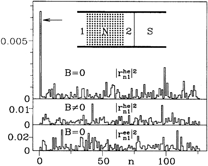
Figure 12: Numerical simulation of a $300\times 300$ tight-binding model for a disordered normal metal, in series with a superconductor (inset). The histograms give the modal distribution for reflection of an electron, with mode number 1 indicating normal incidence. The top two panels give the distribution of reflected holes (in the absence and presence of a magnetic field $B$), the bottom panel of reflected electrons (for $B=0$). The arrow indicates the ensemble-averaged height of the giant backscattering peak for Andreev reflection, predicted from theory. From [30].

.

IX.5.2 Supercurrents

Another important question that can be considered is the current-phase relation for the supercurrent that can flow in-between two superconductors [101]. This is not strictly speaking quantum transport since the supercurrent actually flows at equilibrium.

Numerical calculations of supercurrents are particularly useful for the self-consistent problem which is usually difficult to address analytically. There are many examples of such calculations including [160, 202, 34]

An interesting aspect of superconducting devices is that when the different superconducting electrodes do not share the same electrochemical potential, the problem becomes effectively time-dependent even though the initial formulation is not. For instance, a DC voltage $V_{b}$ across a superconducting-normal-superconducting junction gives rise to an AC current at frequency $2eV_{b}/h$ – this is the AC Josephson effect. To simulate such problems, one need to leave the DC framework of this article and uses time-dependent techniques [66, 222, 267, 305].

IX.5.3 Search for Majorana bound states in nanowires

Majorana bound states (MBSs) are the simplest example of non-Abelian anyons [198]. They have been predicted to be realized for instance in one-dimensional hybrid superconducting/semiconducting nanowire. The simplest model describing such a system is the Bogoliubov-de Gennes Hamiltonian

$$H=\left(\frac{p_{x}^{2}}{2m}-\mu+V(x)+\frac{\alpha_{R}}{\hbar}p_{x}\sigma_{y}\right)\tau_{z}+E_{Z}\sigma_{x}\tau_{0}+\Delta\tau_{x},$$ (225)

where $\sigma_{i}$ ($\tau_{i}$) are Pauli matrices in spin (electron-hole) space, $i=0,x,y,z$. $p_{x}$ is the momentum along the nanowire, $m$ the effective mass of the semiconductor, $\mu$ the global chemical potential, and $V(x)$ a potential induced for example by external gates, allowing to change the electron density in different parts of the wire and defining a tunnel barrier. $\alpha_{R}$ is the strength of Rashba spin-orbit coupling in the semiconductor, $E_{Z}$ the Zeeman splitting induced by an external magnetic field along the nanowire, and $\Delta$ the induced superconducting gap. This model exhibits MBSs when $E_{Z}^{2}>(\mu-V_{\text{wire}})^{2}+\Delta^{2}$, in a region with potential $V_{\text{wire}}$ [178, 207]. Arising through topological phase transition, the appearance of a MBS is always accompanied by a gap closing at the transition point.

Many transport simulations rely on this simple model, but it has also been extended to higher spatial dimensions, including additional physical effects such as the orbital effects of a magnetic field [201], a more realistic modeling of the proximity effect [17, 235], and including all these effects together with electrostatic simulations [308].

Experimental and theoretical work in this field is numerous, and previous experimental results are nowadays discussed controversially. Here we only highlight selected work employing numerical transport simulations that shaped the understanding in this field: MBSs are states at zero-energy, and give rise to a zero-bias peak in transport. However, the particular appearance may depend on device details. Moreover, zero-bias peaks are not specific to MBSs. Numerical transport simulations have been crucial in shaping the understanding of these aspects.

Early work focused on studying the appearance of the zero-bias peak in different device geometries [228, 231]. It was also shown that the gap closing accompanying the appearance of MBS may not be visible in transport measurements [264, 225].

Numerical transport simulations have been essential in shaping the understanding that zero-bias peaks are not a smoking-gun signature of MBSs. Early work showed that disorder can lead to trivial low-lying Andreev bound states giving rise to zero-bias peaks in the conductance [172, 226, 231]. Fig. 13 shows one example of such zero-bias peaks sticking to zero energy even in a trivial system. Later, it was shown that even in the absence of disorder particular Andreev bound states can appear very similar to MBS [171], mimicking for example quantized conductance signatures [194], that previously were considered a smoking gun. Even more, it was shown that any local measurement signal associated with MBSs can be mimicked by trivial states [292]. For this reason, new measurement paradigms have been proposed, in particular non-local measurements to detect the topological phase transition [239, 68].

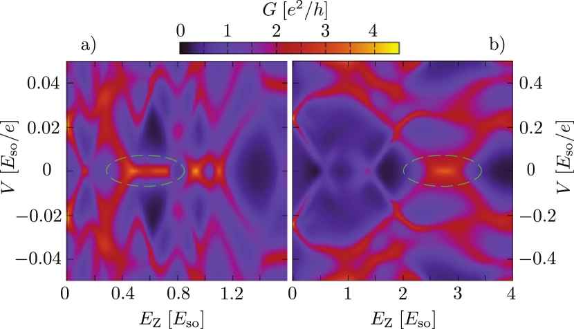
Figure 13: Numerical simulation of a two-dimensional version of Eq.(225) for a nanowire including a tunnel barrier and disorder. The differential conductance is shown for a single disorder realization as a function of bias voltage $V$ and Zeeman splitting $E_{Z}$ due to a parallel magnetic field. The system is in the trivial regime, but still exhibits a conductance peak pinned to zero voltage (green circles) that could be mistaken for a Majorana bound state. The two panels correspond to two parameter regimes. From [226].

IX.6 Spintronics

Quantum transport numerics is also used widely in spintronics. The techniques can be used for mainstream metallic multilayers [37] but have been particularly popular in semiconducting spintronics [81].

A typical Hamiltonian considered in model calculations includes a Rashba spin-orbit coupling term of strength $\alpha$ and ferromagnetic regions with an exchange coupling $J$ and a magnetization oriented around $\vec{m}$:

$$H=\frac{1}{2M}(p_{x}^{2}+p_{y}^{2})+\alpha(p_{y}\sigma_{x}-p_{x}\sigma_{y})$$

$$+J(\vec{r})\vec{m}\cdot\vec{\sigma}.$$ (226)

This type of models can be used to study a variety of phenomena such as the spin Hall effect for electrons [204] or holes [109].

Spintronics studies are not limited to 2D but also include various 3D calculations such as, e.g., 3D topological insulators [59].

IX.7 Self-consistent quantum-electrostatic simulations of nanoelectronics

The model calculations discussed previously assume a known Hamiltonian, i.e., that the electric potential seen by the conducting electrons is an input of the model. This level of modeling is sufficient in many situations but suffers from a number of limitations: the chosen potential may be unrealistic, the relations between the electric potential and, e.g., the voltage applied to electrostatic gate may be unknown, or they may ignore important effects such as edge state reconstruction or non-linear corrections to the conductance. The next level in modeling thus consists in calculating the electric potential self-consistently by solving the quantum problem (the focus of this review) together with the Poisson equation. Below, we review the main aspects of the self-consistent problem.

IX.7.1 Formulation of the self-consistent problem

The self-consistent problem is formulated as a set of three equations that account, respectively, for quantum mechanics, statistical physics, and electrostatics. We denote the electric potential as $U$ and for simplicity suppose that the tight-binding model is formulated in real space (otherwise $U$ has to be replaced by the corresponding matrix elements in the quantum problem). We write $H_{0}$ for the tight-binding Hamiltonian without electric potential and $\Psi_{\alpha E}$ for the scattering state in mode $\alpha$ and energy $E$ (ignoring for simplicity possible bound states present in the system). The problem reads

$$\left[H_{0}-eU\right]\Psi_{\alpha E}=E\Psi_{\alpha E},$$ (227)

$$n=\int\frac{dE}{2\pi}\sum_{\alpha}|\Psi_{\alpha E}|^{2}f_{\alpha}(E),$$ (228)

$$\vec{\nabla}\cdot(\epsilon\vec{\nabla}U)=en+en_{0},$$ (229)

where Eq. (227) is the scattering problem formulated at the beginning of this review. Eq. (228) relates the electronic density $n$ to the local density of states $|\Psi_{\alpha E}|^{2}/(2\pi)$ in a non-equilibrium situation where different leads may have different chemical potentials or temperatures. Eq. (229) is the Poisson equation in a (possibly spatially dependent) dielectric constant $\epsilon$, $e$ is the electron charge, and $n_{0}$ an additional electronic density due to, e.g., dopants.

The self-consistent quantum-electrostatic problem in the presence of electrodes is a non-linear integro-differential problem. Its solution is usually obtained by some sort of iterative scheme. One starts with an initial electronic density, calculates the potential from the Poisson equation, then solves the quantum problem to recalculate the density. This sequence is iterated until convergence. Many techniques have been developed to obtain better convergence properties for such schemes. We refer to [19] for an entrance point to the corresponding literature. Besides the convergence of the self-consistent loop, the calculation of the density itself, Eq. (228) can be computationally intensive. To accelerate the computation, it is useful to separate the density into the sum an equilibrium contribution and an out-of-equilibrium one. The calculation of the equilibrium density can be accelerated using integration in the complex plane [211, 128] while the integration of the out-of-equilibrium contribution spans a small range of energies close to the Fermi energy [251].

The importance of taking into account electrostatics can be illustrated by the non-linear part of the current-voltage characteristics $I(V)$ of a device [61]. Let us write $g_{2}$ for the second-order contribution such that $I(V)=gV+g_{2}V^{2}+\mathcal{O}(V^{3})$. The non-interacting Landauer theory then gives $g_{2}=\frac{1}{2}\frac{\partial g}{\partial E_{F}}$ with $g_{2}(B)=g_{2}(-B)$ in presence of magnetic field. When taking electrostatics into account, one needs to calculate the emissivity $\frac{\partial n_{i}}{\partial V}$ (change of density due to the bias voltage, also known as Landauer dipole), then compute the change of potential $\frac{\partial U_{i}}{\partial n_{j}}$ due to the change of density $n_{j}$ (through Poisson equation), then finally compute the injectivity, i.e., the change of conductance $\frac{\partial g}{\partial U_{i}}$ due to the change of potential. One arrives at

$$g_{2}=\frac{1}{2}\frac{\partial g}{\partial E_{F}}+\sum_{ij}\frac{\partial g}{\partial U_{i}}\frac{\partial U_{i}}{\partial n_{j}}\frac{\partial n_{j}}{\partial V},$$ (230)

where the second terms is entirely due to electron-electron interactions [16, 227, 113]. In particular the antisymmetric part $g_{2}(B)-g_{2}(-B)$ vanishes in the absence of this term.

IX.7.2 Examples of applications

Quantum transport within the self-consistent quantum electrostatic model has been studied in many situations. (Self-consistent calculations within the density functional theory framework will be discussed in the next section.) They are particularly important for the quantum Hall effect as the electrostatic interaction leads to a reconstruction of the edge states into compressible and incompressible stripes [247, 19, 20], as shown in Fig. 14. The technique has also been applied to address silicon devices including quantum dots [94] and transistors [134, 205, 150]. Other calculations have focused on semiconductor nanowires used in the search for Majorana bound states [291, 17, 310].

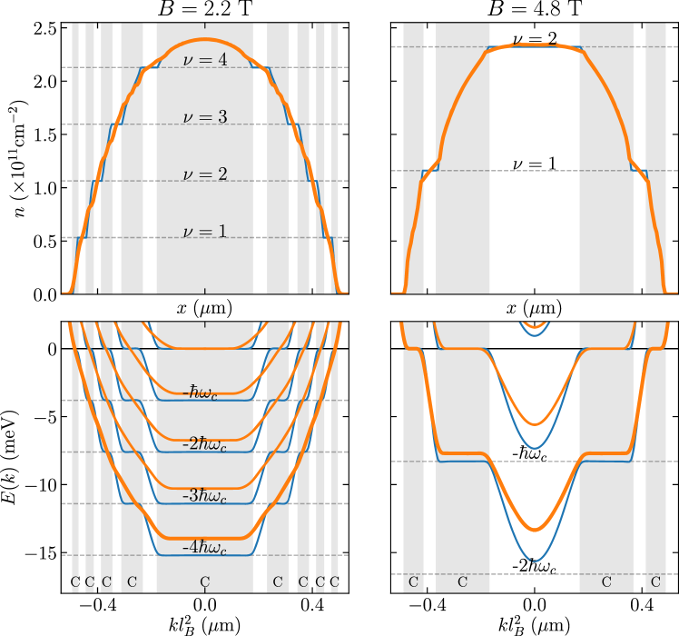
Figure 14: Numerical calculation of the electron density (top) and band structure (bottom) for a top gate-defined wire in a two-dimensional electron gas in the quantum Hall regime. The device is invariant by translation along $y$, the electrons are confined by two gates along $x$ with the magnetic field applied along $z$. Blue lines correspond to a self-consistent Thomas-Fermi calculation, orange lines to a full solution of the Poisson-Schrödinger problem. Gray regions indicate the compressible stripes while the white regions are incompressible. Adapted from [20].

X Selected applications to realistic systems

In this section, we turn to a few applications of computational quantum transport for “realistic” models, i.e., the DFT, FP-TBM and SE-TBM discussed in Fig. IX.1. Once again, we do not aim at being exhaustive, the corresponding literature being very large, but just point to a few illustrative cases.

X.1 DFT models

First-principles density functional theory (DFT) can provide predictive calculations in the absence of any prior experimental data. The combined approach is often referred to as DFT + NEGF. There exist many reviews and pedagogical materials that explain DFT in great detail. We refer the interested reader to the articles that accompany DFT software packages, a list of which can be found towards the end of Sec. I.2.

X.1.1 Non-linear conductance in short junctions

We start with a use case where density functional theory (DFT) is used to compute the non-linear current voltage characteristics of nanodevices. As we have seen in the preceding section, it is crucial to treat the electron-electron interaction at least at the mean field level to calculate non-linear corrections to the conductance. DFT calculations do that by design and have been used in many situations [251].

Early calculations and later benchmarks focused on short wires made of a few atoms, e.g., C, Al or Au [154, 42, 214, 238]. The calculations soon extended to molecular nanoelectronics [76, 131, 82, 86, 246]. Despite the sensitivity of the conductance to the nature of the molecule-electrode contact, it was found in [75] that the qualitative shape of the experimental $I-V$ characteristics could be recovered. Another topic that attracted a strong interest is carbon nanotubes [275] as well as graphene-based devices with either a transistor-like geometry [212, 18, 216] or multi-terminal cross bar geometry [38, 106, 243]. Possible applications of these devices include DNA sensing using nanopores in graphene [245]. Recent works have extended the studies to other 2D materials such as MoS₂ [95]

Despite their widespread use, it should be noted that these DFT techniques have serious limitations for the study of small junctions. Perhaps the most important one is that these techniques do not account for the ubiquitous phenomena of Coulomb blockade. Another limitation is that most studies ignore phonons and more generally atomic displacements that may be triggered by the out-of-equilibrium situation. In the presence of bound states, an additional prescription must be given to determine their occupations [164]. In some situations, it is important to properly account for the charge redistribution rather deeply inside the electrodes [192].

X.1.2 Applications to spintronics

A very successful example of the DFT + NEGF approach is the theoretical prediction [46, 190] of the existence of a large tunneling magneto-resistance of a Fe/MgO/Fe magnetic tunnel junction. There, the coherent spin-polarized tunneling and the symmetry of electron wave functions plays an essential role that can only be captured by quantum transport calculations. This prediction has motivated large experimental efforts [313] to fabricate such devices. These magnetic tunnel junctions now play a central role in both basic [298] and applied [173] spintronics research.

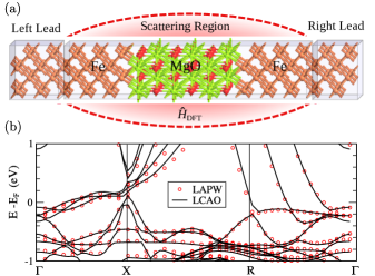
Figure 15: (a) Schematic view of a magnetic tunnel junction where 6 monolayers of MgO(001) insulating barrier are sandwiched between two semi-infinite Fe(001) leads. The junction is infinite in the transverse direction, so that the depicted supercell is periodically repeated in the direction transverse to current flow from the left to the right Fe lead. (b) Electronic band structure of a periodic Fe/MgO/Fe/MgO…Fe/MgO lattice obtained by DFT calculations using LCAO basis (solid line) versus those using full potential linearized augmented plane-wave basis (circles). Panel (b) is adapted from [295].

Fig. 15a shows a schematic of a Fe-MgO-Fe junction simulated in [295]. The system is supposed to be invariant by translation along the direction perpendicular to the junction (no disorder) so that the transmission is calculated as a function of the transverse momentum which must be integrated upon at the end of the calculation. The Hamiltonian of the scattering region was written in a linear combination of atomic orbitals (LCAO). An accurate calculations requires as many as 10 000 orbitals for this calculation while the supercell only contains a total of 24 atoms (Fe Mg and O). To control this accuracy, one compares the LCAO calculation with a more accurate one done in a plane wave basis, as illustrated in Fig. 15b. In addition to checking the convergence of the calculation with the number of LCAO orbitals, one must also obtain convergence of the momentum integration which requires $\sim 10^{4}$ momentum points at zero bias (only $\sim 10^{2}$ for the band structure, up to $\sim 10^{5}$ at finite bias voltage, up to $\sim 10^{7}$ for spin-torque [299]).

Later works tried to optimize the magneto-resistance of the tunnel junction. It has been predicted, for instance, that a few layers of graphene with Ni electrodes act as a perfect spin filter [127] with regimes showing a negative differential resistance [244] at finite bias. Another line of work used DFT+NEGF to address metallic magnetic systems [254, 269]. An important evolution of the field has been the discovery of the phenomena of spin-transfer torque in non-collinear systems. Spin torque has enabled fully electric control of a magnetic configuration [232]. DFT studies of spin transfer torque include [269, 108, 299, 79]. Recent studies also capture a related effect, the spin orbit torque [203].

X.2 First-principles tight-binding models (FP-TBM)

The direct DFT approach to quantum transport is very computationally intensive. These calculations are usually restricted to one-dimensional systems or quasi-one-dimensional systems that are invariant by translation along the perpendicular direction. For more complex geometries or in the presence of disorder [132, 312] one needs to develop effective models that reduce the complexity. The FP-TBM approach projects the DFT Hamiltonian onto a smaller basis set, typically atomic or pseudo-atomic orbitals. FP-TBM are designed to describe the physics in a finite energy window centered around the Fermi level. We distinguish FP-TBM (where there exists a systematic procedure to construct the basis set) from the semi-empirical SE-TBM discussed in the next subsection, where the construction is less systematic. The systematic approach of FP-TBM methods is particularly important when several bands get hybridized at the Fermi level.

Perhaps the most well-known FP-TBM basis are the maximally localized Wannier functions which can be constructed out of Bloch wave functions [188]. These orbitals are rather compact, retain the original symmetries of the bands and reproduce well the original DFT results. A popular approach uses a plane wave code such as VASP [143] followed by a projection on Wannier orbitals using, e.g., the code Wannier90 [196]. An illustrative example is the case of graphene. Using a minimal basis set of a single $p_{z}$-like orbital per site, [84] find that including hoppings up to the 8^th neighbor (i.e., 400 parameters) is required to reproduce the bands predicted by DFT. This can be contrasted with the single parameter model used in the preceding section. Examples of quantum transport calculations performed with Wannier functions include the calculation of the conductance of disordered nanowires [53, 257] and of single molecule junctions [279, 272].

An alternative to Wannier function uses the linear-muffin-tin-orbitals (LMTO) and its generalizations [13]. Other FP-TBM include the quasiminimal basis orbitals [297] or predetermined basis of fixed localized wave functions [2, 3]. All these techniques require particular care in the treatment of boundaries or interfaces if the model is to be transferred to other geometries or structures.

X.3 Semi-empirical tight-binding models (SE-TBM)

Continuing with the hierarchy of Hamiltonians, we now consider semi-empirical tight-binding models (SE-TBM). In this approach a set of relevant orbitals and couplings is chosen a priori. The model is then fitted to ab-initio data (e.g., often to reproduce the DFT band structure) and/or to reproduce experimental data. SE-TBM models can have up to hundreds of parameters. The simplest SE-TBM models, with very few parameters, essentially match the model Hamiltonians discussed in the preceding section. The SE-TBM models are also closely connected to the $\mathbf{k}\cdot\mathbf{p}$ models discussed in the next subsection. The main difficulty in preparing SE-TBM for quantum transport calculations is the same as the one discussed in the preceding section for FP-TBM models: a proper treatment of the boundaries of the device and the interface between different materials. For instance, the description of the interface between graphene and metallic contacts can require as many as hundred parameters for a faithful description [215, 28]. The models are usually fitted with classical least mean square optimization methods, but recently machine learning approaches have started to be used [112].

SE-TBM models are extremely popular and we cannot do justice to the literature in this review. They have been applied to MoS₂ devices [237], adatoms on graphene [301], graphene-hBN devices [185], quantum dots [177], 3D topological insulators Bi₂Se₃, Bi₂Te₃, Sb₂Te₃ [170], and many more. Let us also mention the possibility to perform multiscale calculations where critical parts of the system are described at the DFT level while other parts use SE-TBM models [52].

X.3.1 Semiconductor devices

SE-TBM models for semiconductors go back to the eighties with minimum next nearest-neighbor models accounting for the s and p orbitals [289]. More accurate models also include the d bands: [54, 39]. Assuming that the hopping matrix elements only depend on the distance between atoms [215], these models can be parametrized as a function of atomic distance and then used for an arbitrary atomic configuration. This is very useful for semiconductor devices where stress can have a significant effect on transport properties [205, 80]. Another appealing aspect of these models is that they can correct typical deficiencies of DFT approaches, e.g., the inability to correctly predict the semi-conductor gap, by fitting the model to experimental data.

X.3.2 Carbon based nanodevices

SE-TBM models are also extremely popular for modeling graphene nanoribons or carbon nanotube devices. It was recognized early on that the simple nearest-neighbor TBM for a single $p_{z}$ orbital Eq. (220) is often inaccurate: it predicts perfectly flat bands in zigzag nanoribons as well as a metallic (gapless) band structure for armchair nanoribbons that are $3N+2$ carbon atoms wide. A more accurate model uses second- and third-nearest-neighbor hoppings [236]. Equivalently, one may use nearest-neighbor hoppings with more bands [65, 41]. These additional bands are also important when describing the spin-orbit interaction [139]. Again, the transport properties across these carbon-based devices are very sensitive to the accuracy of model and in particular the interfaces. For instance, SE-TBM modeling [180] that did not properly address the interface between carbon nanotubes and the metallic Ohmic contact could not predict the experimental findings quantitatively [89]. Another example is the off current of graphene nanoribbon transistors which varies by orders of magnitude upon moving from the simple single-orbital $p_{z}$-SETBH model to a more elaborate multi-orbital $p/d$-SETBH model [41]. Similar conclusions were drawn for the validity of simulations of non-local resistances in graphene Hall bars [185].

X.4 Discretized $\mathbf{k}\cdot\mathbf{p}$ Hamiltonians

We end our hierarchy of realistic models with $\mathbf{k}\cdot\mathbf{p}$ Hamiltonians. The $\mathbf{k}\cdot\mathbf{p}$ Hamiltonians are low-energy effective theories valid in the vicinity of some high-symmetry $k$-point. They describe the physics at large scale, not at the atomic scale, which can be advantageous for the simulation of large systems. There exists a large literature on the $\mathbf{k}\cdot\mathbf{p}$ method [290]. [140] describes the particular case of two-dimensional transition metal dichalcogenide semiconductors while [184] focuses on graphene. $\mathbf{k}\cdot\mathbf{p}$ Hamiltonians can account for magnetic field as well as spin-orbit effects [309].

In the simplest cases, $\mathbf{k}\cdot\mathbf{p}$ models often reduce to the model Hamiltonians discussed in the preceding section. For instance, the effective-mass approximation can be thought as arising from developing the dispersion relation around the $\Gamma$ point of the conductance band of a III-V semiconductor. In the case of graphene, the simple tight-binding model Eq. (220) can be expanded around the two points $K$ and $K^{\prime}$ of the Brillouin zone which leads to two copies of the 2D massless Dirac equation Eq. (221). More complex examples arise in the description of semi-conductors and in particular to account for the $p$-character of their valence band. For instance, the $4\times 4$ Luttinger Hamiltonian [179],

$$H=\frac{1}{2m}\left[\left(\gamma_{1}+\frac{5}{2}\gamma_{2}\right)\hat{\mathbf{p}}^{2}-2\gamma_{2}\left(\hat{\mathbf{p}}\cdot\hat{\mathbf{S}}\right)^{2}\right],$$ (231)

describes the heavy and light hole bands of semi-conductors. Here $m$ is the electron mass and $\hat{\mathbf{S}}=(S_{x},S_{y},S_{z})$ is a vector of spin-3/2 operators. The dimensionless parameters $\gamma_{1}$ and $\gamma_{2}$ are material specific. Prior to quantum transport calculations, these models must be discretized using, e.g., finite differences. When discretizing these models, particular care needs to be taken to avoid spurious solutions, e.g., in $8\times 8$ $\mathbf{k}\cdot\mathbf{p}$ semiconductor models [88]. Additionally, Dirac materials are not amenable to regular discretization due to the occurrence of the fermion doubling problem as explained in Sec. IX.3.2. $\mathbf{k}\cdot\mathbf{p}$ models are often used for quantum transport calculations such as [311, 260]. As for other models, special care must be given to the treatment of boundaries and interfaces [45] so that they are error prone when used for confined structures such as quantum dots [90] or thin films [199].

XI Final remarks

XI.1 Simulation workflow

In practice, numerical simulations of quantum transport devices are often carried out by approaching the complete problem step by step. One starts by studying the bulk Hamiltonian(s) for the material(s) under consideration. Written in $k$-space, these Hamiltonians are readily diagonalized and their spectrums provides useful information such as the positions of gaps or Dirac points.

In a second step, one constructs electrodes of finite width and analyzes them in isolation. The associated $k$-space Hamiltonians provide information such as the number of propagating modes in each electrode. Packages such as KwantSpectrum [137] provide tools to facilitate this analysis.

It is only in a third step that one proceeds to treating scattering problems that consist of a scattering region with attached electrodes. It it often useful to start out with subparts of the final device. For instance, in an electronic interferometer that contains several quantum point contacts, one could study the transport properties of a system that contains a single quantum point contact in order to calibrate the corresponding model. Another example is the interface between two materials that could be studied separately before being integrated into a larger device. When the final device is very large, it can actually be computationally advantageous to stop at this level and concatenate the scattering matrices of the different pieces numerically (following, e.g., [241]). In most cases, however, one proceeds, at last, to simulate the entire device directly.

While in former times research groups relied on in-house codes, nowadays in most cases one will want to take advantage of already existing solutions, at least as a starting point or foundation. Out of the codes that are listed at the end of Sec. I.2, the following three target quantum transport specifically and are under active maintenance: nextnano [33], Kwant [104], and Quantica.jl [249].

XI.2 Outlook

Numerical calculations of quantum transport have become an ubiquitous tool in many fields, from electrical engineering to materials science and quantum nanoelectronics. In this review, we focused on providing a comprehensive presentation of the two equivalent formalisms used in this field, the scattering matrix approach and the Green’s function approach, with an emphasis on explicitly providing the links between the two. We also provided an in-depth review of the different algorithms that have been developed to perform actual calculations.

Many topics fall beyond the scope of this review. One is the simulation of time-dependent quantum transport [265, 145, 137], see [97] for a review, and its special case of finite-frequency transport or Floquet scattering [195]. Another major aspect that we did not touch is the effect of electron-electron interactions or the interaction of electrons with other degrees of freedom such as phonons or magnons. It is indeed a very frustrating fact that even the simplest and most common of these effects, for instance Coulomb blockade, cannot be easily incorporated into the type of approach presented in this review. The effects of decoherence are also beyond the scope of this review.

In terms of applications, the range is so vast that we could only point to a few examples. Our choice of topics was necessarily subjective and biased by our own interests.

With regard to future work, much remains to be done besides addressing the above points. One important aspect is improving the accuracy of predictions compared to experiments [60]. This requires better models, efficient tools to address electrostatics, solvers capable to handle large systems (in particular in three dimensions), and close collaboration with experimental teams with the goal of producing systematic data sets dedicated to the calibration of models.

Author contributions

AA, MW, and XW developed the formalism. AA and MW developed the stable algorithm for solving the scattering problem. MI described the bound state problem. TOR and DV implemented and described symmetry analysis of the modes. BKN wrote the section on applications to realistic systems. AA, MW, CG, and XW wrote the rest of the manuscript. XW organized the writing. All authors reviewed the text.

Appendix A Derivation of Feynman-Hellman equation for the velocity

The Feynman-Hellman equation relates the velocity of a mode to the average of the velocity operator. Considering normalized modes,

$$\phi^{\dagger}\phi=1$$ (232)

we have

$$\frac{\partial\phi^{\dagger}}{\partial k}\phi+\phi^{\dagger}\frac{\partial\phi}{\partial k}=0.$$ (233)

From $E(k)=\phi^{\dagger}H(k)\phi$ we get,

$$v \equiv \frac{\partial E(k)}{\partial k}$$ (234)

$$= \frac{\partial\phi^{\dagger}}{\partial k}H(k)\phi+\phi^{\dagger}H(k)\frac{\partial\phi}{\partial k}+\phi^{\dagger}\frac{\partial H(k)}{\partial k}\phi$$

$$= E(k)\left[\frac{\partial\phi^{\dagger}}{\partial k}\phi+\phi^{\dagger}\frac{\partial\phi}{\partial k}\right]+\phi^{\dagger}\frac{\partial H(k)}{\partial k}\phi$$

$$= \phi^{\dagger}\frac{\partial H(k)}{\partial k}\phi$$

$$= i\phi^{\dagger}\left[\lambda V^{\dagger}-\lambda^{-1}V\right]\phi$$

which is the Feynman-Hellman equation. Note that inside the matrices $\Phi$, the modes $\phi$ are renormalized to carry a unit velocity $v=\pm 1$.

Appendix B Properties of the leads modes.

In this appendix, we establish a few technical results on the lead propagating and evanescent modes that are needed in various proofs of the main text. We begin by multiplying Eq. (37) by $\Phi^{\dagger}$:

$$\Phi^{\dagger}V\Phi+\Phi^{\dagger}(H-E)\Phi\Lambda+\Phi^{\dagger}V^{\dagger}\Phi(\Lambda)^{2}=0.$$ (235)

The complex conjugate of the above equation reads

$$(\Lambda^{*})^{2}\Phi^{\dagger}V\Phi+\Lambda^{*}\Phi^{\dagger}(H-E)\Phi+\Phi^{\dagger}V^{\dagger}\Phi=0.$$ (236)

Now, multiplying Eq. (235) by $\Lambda^{*}$ on the left and Eq. (236) by $\Lambda$ on the right, we arrive after subtracting one equation from the other at

$$[\lambda_{\alpha}^{*}-(\lambda_{\alpha}^{*})^{2}\lambda_{\beta}]\left.\Phi^{\dagger}V\Phi\right|_{\alpha\beta}=[-\lambda_{\alpha}^{*}(\lambda_{\beta})^{2}+\lambda_{\beta}]\left.\Phi^{\dagger}V^{\dagger}\Phi\right|_{\alpha\beta}.$$ (237)

which is valid for all types of modes, evanescent and/or propagating.

B.1 Application to evanescent modes

If one of the two modes $\alpha$ or $\beta$ is evanescent, we can simplify Eq. (237) by $1-\lambda_{\alpha}^{*}\lambda_{\beta}\neq 0$ and arrive at

$$\lambda_{\alpha}^{*}\left.\Phi^{\dagger}V\Phi\right|_{\alpha\beta}=\lambda_{\beta}\left.\Phi^{\dagger}V^{\dagger}\Phi\right|_{\alpha\beta}$$ (238)

which can be written in matrix form as,

$$\Lambda_{\mathrm{e}+}^{*}\Phi_{\mathrm{e}+}^{\dagger}V\Phi_{\mathrm{e}+}=\Phi_{\mathrm{e}+}^{\dagger}V^{\dagger}\Phi_{\mathrm{e}+}\Lambda_{\mathrm{e}+}$$ (239)

Similarly,

$$\Lambda_{\mathrm{p}+}^{*}\Phi_{\mathrm{p}+}^{\dagger}V\Phi_{\mathrm{e}+}=\Phi_{\mathrm{p}+}^{\dagger}V^{\dagger}\Phi_{\mathrm{e}+}\Lambda_{\mathrm{e}+}$$ (240)

and

$$\Lambda_{\mathrm{e}+}^{*}\Phi_{\mathrm{e}+}^{\dagger}V\Phi_{\mathrm{p}+}=\Phi_{\mathrm{e}+}^{\dagger}V^{\dagger}\Phi_{\mathrm{p}+}\Lambda_{\mathrm{p}+}$$ (241)

B.2 Application to propagating modes

For propagating modes $1-\lambda_{\alpha}^{*}\lambda_{\beta}$ vanishes whenever $\lambda_{\alpha}=\lambda_{\beta}=\lambda$, i.e., the two modes $\alpha$ and $\beta$ have the same momentum. In that situation, we can form the velocity matrix

$$i\Phi_{\mathrm{p}+}^{\dagger}\left[\lambda V^{\dagger}-\lambda^{*}V\right]\Phi_{\mathrm{p}+}|_{\alpha\beta}$$ (242)

where $\alpha$ and $\beta$ lie inside the degenerate space. This matrix is Hermitian hence can be diagonalized. The resulting linear combination of propagating modes (for which we abusively use the same notation), normalized to carry unit velocities remain solutions of the mode equation and further satisfy,

$$i\Phi_{\mathrm{p}+}^{\dagger}\left[\lambda V^{\dagger}-\lambda^{*}V\right]\Phi_{\mathrm{p}+}|_{\alpha\beta}=\delta_{\alpha\beta}$$ (243)

from which we finally get,

$$\Lambda_{\mathrm{p}+}^{*}\Phi_{\mathrm{p}+}^{\dagger}V\Phi_{\mathrm{p}+}=\Phi_{\mathrm{p}+}^{\dagger}V^{\dagger}\Phi_{\mathrm{p}+}\Lambda_{\mathrm{p}+}+i$$ (244)

A corresponding expression can be derived for incoming modes. In that case, the sign of the current is opposite and one arrives at,

$$\Lambda_{\mathrm{p}-}^{*}\Phi_{\mathrm{p}-}^{\dagger}V\Phi_{\mathrm{p}-}=\Phi_{\mathrm{p}-}^{\dagger}V^{\dagger}\Phi_{\mathrm{p}-}\Lambda_{\mathrm{p}-}-i$$ (245)

Appendix C Proof of invertibility of mode matrices

In this section, we discuss the relation between the rank of $\Phi_{\bar{t}+}$ and the absence of bound state in the corresponding semi-infinite lead.

Let us suppose that $\Phi_{\bar{t}+}$ is not full rank. It follows that $V\Phi_{\bar{t}+}$ is not full rank neither, hence that there is a vector $c\neq 0$ such that $V\Phi_{\bar{t}+}c=0$. On the other hand, we know that the wave function

$$\psi(j)=\Phi_{\bar{t}+}\Lambda_{\bar{t}+}^{j}c$$ (246)

is an eigenstate of the infinite lead, i.e., it satisfies the infinite lead equation

$$V\psi(j-1)+(H-E)\psi(j)+V^{\dagger}\psi(j+1)=0.$$ (247)

In addition, we now have $V\phi(0)=0$, which means that $\psi(j)$ also fulfills the boundary condition,

$$(H-E)\psi(1)+V^{\dagger}\psi(2)=0.$$ (248)

In other words, $\psi(j)$ is an eigenstate of the semi-infinite lead.

Let us now decomposes the vector $c$ into its propagating and evanescent sector $c=(c_{\mathrm{p+}},c_{\mathrm{\bar{e}+}})$. Using Eq.(239) and Eq.(244), we get,

$$c^{\dagger}\Lambda_{\bar{t}+}^{*}\Phi_{\bar{t}+}^{\dagger}V\Phi_{\bar{t}+}c=c^{\dagger}\Phi_{\bar{t}+}^{\dagger}V^{\dagger}\Phi_{\bar{t}+}\Lambda_{\bar{t}+}c+ic_{\mathrm{p+}}^{\dagger}c_{\mathrm{p+}}$$ (249)

and since $V\Phi_{\bar{t}+}c=c^{\dagger}\Phi_{\bar{t}+}^{\dagger}V^{\dagger}=0$, it follows that $c_{\mathrm{p+}}^{\dagger}c_{\mathrm{p+}}=0$ hence,

$$c_{\mathrm{p+}}=0$$ (250)

Hence, $V\Phi_{\mathrm{t}+}c=0$ reduces to $V\Phi_{\mathrm{e}+}c_{\bar{e}+}=0$ which in turns means that $\psi(j)$ is a bound state solution of the semi-infinite lead. This last paragraph is a technical way to reflect the fact that the probability current of an eigenstate of the semi-infinite lead must be zero everywhere - this is current conservation - hence the propagating contribution must vanish since we include only modes that propagate along one direction.

Conversely, if there are no bound states at energy $E$, then $V\Phi_{\bar{t}+}$ is full rank. Since $V=AB^{\dagger}$, $V\Phi_{\bar{t}+}$ being full rank implies that $B^{\dagger}\Phi_{\bar{t}+}$ is full rank and since it is a square matrix, it must therefore be invertible.

Appendix D Scattering problem with non-orthogonal basis set

This review has focused on tight-binding models with an orthogonal basis set. However, non-orthogonal basis sets appear naturally for basis sets used in Slater-Koster tight-binding methods or density functional theory, as, e.g., in [124, 209, 210, 215]. In this case, different basis states $\left|n_{i}\right>$ have finite overlap, $\left\langle n_{i}|n_{j}\right\rangle=W_{ij}$. Note that usually the overlap matrix is denoted by the letter $S$ which is already taken by a central object of this review, the scattering matrix. Hence we resort to $W$ to denote the overlap matrix.

In this appendix we will argue how the main formulas presented in this review can be generalized to tight-binding models with a non-orthogonal basis set with a simple replacement rule. More explicit and extensive derivations can be found in the literature, such as for the Green’s function formalism in [174] and its non-equilibrium version in [151].

The Schrödinger equation for the scattering system with a non-orthogonal basis reads

$$\hat{H}_{\text{sys}}\hat{\psi}=E\hat{W}_{\text{sys}}\hat{\psi}$$ (251)

with the overlap matrix

$$W_{\text{sys}}=\begin{pmatrix}W_{\text{sr}}&P_{\text{sr}}^{T}W_{V}^{\dagger}&\\ W_{V}P_{\text{sr}}&W_{H}&W_{V}^{\dagger}\\ &W_{V}&W_{H}&W_{V}^{\dagger}\\ &&W_{V}&W_{H}&W_{V}^{\dagger}\\ &&&\ddots&\ddots&\ddots\end{pmatrix},$$ (252)

where $W_{\text{sr}}^{\dagger}=W_{\text{sr}}$ and $W_{H}^{\dagger}=W_{H}$ by definition. Here we have also assumed that the overlap matrix $W_{\text{sys}}$ has the same sparsity structure as the Hamiltonian $H_{\text{sys}}$, which can always be achieved by choosing the unit cell of the leads appropriately.

Most of the results in this review are obtained by direct manipulation of the Schrödinger equation $\hat{H}_{\text{sys}}\hat{\psi}=E\hat{\psi}$. To generalize to the case of a non-orthogonal basis, i.e., (251), it is thus sufficient to replace

$$\begin{split}H_{\text{sr}}-E&\rightarrow H_{\text{sr}}-E\,W_{\text{sr}},\\ H-E&\rightarrow H-E\,W_{H}\text{, and}\\ V&\rightarrow V-E\,W_{V}\end{split}$$ (253)

in our main results such as Eq.(50).

The Bloch equation for the lead modes now reads

$$H(k)\phi=E(k)W(k)\phi$$ (254)

with $W(k)=W_{V}e^{-ik}+W_{H}+W_{V}^{\dagger}e^{ik}$. In analogy to Appendix A, the expression of the velocity of a lead mode is obtained by projecting the equation on $\phi^{\dagger}$ and taking a derivative with respect to $k$. This yields

$$v=\frac{1}{\hbar}\frac{dE}{dk}=\frac{i}{w}\phi^{\dagger}\left[\lambda(V^{\dagger}-EW_{V}^{\dagger})-\lambda^{-1}(V-EW_{V})\right]\phi,$$ (255)

where $w=\phi^{\dagger}(\lambda W_{V}^{\dagger}+W_{H}+\lambda^{-1}W_{V})\phi$, and again $\lambda=e^{ik}$. In our derivations we used the convention that propagating modes are normalized such that $v=1$. Hence, for the case of a non-orthogonal basis set, we need to absorb both $v$ and $w$ in the normalization of $\phi$. With this convention, the properties of the lead modes derived in Appendix B hold with the replacement rules (253), as they are again obtained by direct manipulation of the Bloch equation in the leads.

Hence, with the replacement rules (253) the results presented in this review can immediately be applied to systems with a non-orthogonal basis set.

Appendix E Notation

$\hat{H}_{\text{sys}}$ / $\hat{G}_{\text{sys}}$ / $\hat{\psi}$	Hamiltonian / Green’s function / Wave function of full (infinite) systems. The hat indicate an infinite system while subscript specifies the system (infinite lead alone $H_{\text{lead}}$ or semi-infinite lead + scattering region $H_{\text{sys}}$.
$\hat{H}_{\text{lead}}$ / $\hat{\phi}$	Hamiltonian / Wave function of the full infinite lead.
$H_{\text{sr}}$ / $G_{\text{sr}}$	Hamiltonian / Green’s function of scattering region
$H$, $V$	Hamiltonian and hopping matrix of lead
$\Sigma$	Lead self-energy
$H(k)$	Bloch Hamiltonian of the lead
$V_{j}$	hopping in lead between j-th nearest neighbor cell ($V=V_{1}+V_{2}+\dots$)
$P_{\text{sr}}$	projection from lead to scattering region
$\Phi$ / $\phi$	matrix of translation eigenvectors (transverse modes) / vector of a single translation eigenvector. The columns of $\Phi$ are made of the $\phi$ vectors.
$\Lambda$ / $\lambda$	matrix of translation eigenvalues / single eigenvalue
$\tilde{\Lambda}$	truncated $\Lambda$ matrix where the vanishing diagonal elements have been disregarded.
p,± / e,±	subscript indicating a propagating ($\mathrm{p}$) / evanescent ($\mathrm{e}$) mode, with $\pm$ indicating whether it’s incoming ($-$, going toward the scattering region) or outgoing ($+$ going away from the scattering region).
t	subscript ($\mathrm{t}$) indicating both propagating ($\mathrm{p}$) and evanescent ($\mathrm{e}$) modes.
${}_{\mathrm{\bar{t}}}$	subscript ($\mathrm{\bar{t}})$ similar to $(\mathrm{t})$ but the modes $\lambda_{\alpha}=0$ are excluded. See Table 1.
${}_{\mathrm{\bar{e}}}$	subscript ($\mathrm{\bar{e}})$ similar to $(\mathrm{e})$ but the modes $\lambda_{\alpha}=0$ are excluded. See Table 1.
$v$	velocity
$J$	current
$N$	number of modes or sites. $N_{\mathrm{t}}=N_{\mathrm{p}}+N_{\mathrm{e}}$ is the number of sites in each unit cell of the lead. $N_{\text{sr}}$ is the number of sites of the scattering region.
$V=AB$	decomposition of the lead hopping matrix
$S$	scattering matrix
$S_{\text{tp}}$	Generalized scattering matrix containing both outgoing propagating and evanescent modes.
$\psi_{\text{sr}}$ / $\Psi_{\text{sr}}$	wave function in scattering region / wave function matrix: the columns of $\Psi_{\text{sr}}$ are made of the vectors $\psi_{\text{sr}}$
$E$, $\varepsilon$	energy
$M$	transfer matrix
$T$	transmission
$g$	conductance
$\Theta$	temperature
$\mu$	chemical potential
$E_{F}$	Fermi energy
$\lambda_{F}$	Fermi wave length
$V_{b}$	Bias voltage
$f(E)$	Fermi function
$I_{a}$	Electric current in lead $a$ (counted positive when flowing towards the scattering region)
$g_{ab}(E)$	Dimensionless conductance matrix between lead $a$ and $b$
$\mathcal{G}_{ab}$	Conductance matrix between lead $a$ and $b$
$r,t$	reflection and transmission matrices
$\Sigma$	self-energy
$P$	projector onto conservation law blocks
$\mathcal{C}$, $\mathcal{P}$, $\mathcal{T}$	chiral, particle-hole, and time-reversal symmetry
$k$	$k$-vector
$q$	vector of amplitudes of the different (propagating/evanescent) modes.
$\alpha,\beta,\gamma,\delta$	Greek letters label mode index.
$n,m$	latin letters label site index.
$i,j$	labels the unit cells within a single lead
$a,b,c,d$	labels different leads
$c_{n}$ and $c^{\dagger}_{n}$	are the fermionic annihilation and creation operators on site $n$.
${\cal H}$	is the second quantized Hamiltonian
$\Theta(\tau)$	is the Heaviside function
$\tau$	is time.
$\eta$	is a small imaginary energy
$BS$	subscript, denote solutions of Eq. (56)
$\mathds{G}$, $\mathds{H}$	are generic Green’s function and Hamiltonian matrices

References

- Abrahams et al. [1979] Abrahams, E, P. W. Anderson, D. C. Licciardello, and T. V. Ramakrishnan (1979), “Scaling theory of localization: Absence of quantum diffusion in two dimensions,” Phys. Rev. Lett. 42, 673–676.
- Agapito et al. [2016a] Agapito, Luis A, Marco Fornari, Davide Ceresoli, Andrea Ferretti, Stefano Curtarolo, and Marco Buongiorno Nardelli (2016a), “Accurate tight-binding Hamiltonians for two-dimensional and layered materials,” Phys. Rev. B 93, 125137.
- Agapito et al. [2016b] Agapito, Luis A, Sohrab Ismail-Beigi, Stefano Curtarolo, Marco Fornari, and Marco Buongiorno Nardelli (2016b), “Accurate tight-binding Hamiltonian matrices from ab initio calculations: Minimal basis sets,” Phys. Rev. B 93, 035104.
- Akhmerov et al. [2011] Akhmerov, A R, J. P. Dahlhaus, F. Hassler, M. Wimmer, and C. W. J. Beenakker (2011), “Quantized conductance at the Majorana phase transition in a disordered superconducting wire,” Phys. Rev. Lett. 106, 057001.
- Akhmerov et al. [2009] Akhmerov, A R, C. W. Groth, J. Tworzydło, and C. W. J. Beenakker (2009), “Switching of electrical current by spin precession in the first Landau level of an inverted-gap semiconductor,” Phys. Rev. B 80, 195320.
- Akkermans and Montambaux [2007] Akkermans, E, and G. Montambaux (2007), Mesoscopic Physics of Electrons and Photons (Cambridge University Press).
- Alhassid [2000] Alhassid, Y (2000), “The statistical theory of quantum dots,” Rev. Mod. Phys. 72, 895–968.
- Allen [1979a] Allen, Roland E (1979a), “Green’s function and generalized phase shift for surface and interface problems,” Phys. Rev. B 19, 917–924.
- Allen [1979b] Allen, Roland E (1979b), “Green’s functions for surface physics,” Phys. Rev. B 20, 1454–1472.
- Amestoy et al. [1996] Amestoy, Patrick R, Timothy A. Davis, and Iain S. Duff (1996), “An approximate minimum degree ordering algorithm,” SIAM Journal on Matrix Analysis and Applications 17 (4), 886–905, https://doi.org/10.1137/S0895479894278952 .
- Amestoy et al. [2019] Amestoy, PR, A. Buttari, J.-Y. L’Excellent, and T. Mary (2019), “Performance and Scalability of the Block Low-Rank Multifrontal Factorization on Multicore Architectures,” ACM Transactions on Mathematical Software 45, 2:1–2:26.
- Amestoy et al. [2001] Amestoy, PR, I. S. Duff, J. Koster, and J.-Y. L’Excellent (2001), “A fully asynchronous multifrontal solver using distributed dynamic scheduling,” SIAM Journal on Matrix Analysis and Applications 23 (1), 15–41.
- Andersen and Saha-Dasgupta [2000] Andersen, O K, and T. Saha-Dasgupta (2000), “Muffin-tin orbitals of arbitrary order,” Phys. Rev. B 62, R16219–R16222.
- Anderson et al. [1999] Anderson, E, Z. Bai, C. Bischof, S. Blackford, J. Demmel, J. Dongarra, J. Du Croz, A. Greenbaum, S. Hammarling, A. McKenney, and D. Sorensen (1999), LAPACK Users’ Guide, 3rd ed. (Society for Industrial and Applied Mathematics, Philadelphia, PA).
- Ando [1991] Ando, T (1991), “Quantum point contacts in magnetic fields,” Phys. Rev. B 44 (15), 8017–8027.
- Angers et al. [2007] Angers, L, E. Zakka-Bajjani, R. Deblock, S. Guéron, H. Bouchiat, A. Cavanna, U. Gennser, and M. Polianski (2007), “Magnetic-field asymmetry of mesoscopic rectification in Aharonov-Bohm rings,” Phys. Rev. B 75, 115309.
- Antipov et al. [2018] Antipov, Andrey E, Arno Bargerbos, Georg W. Winkler, Bela Bauer, Enrico Rossi, and Roman M. Lutchyn (2018), “Effects of gate-induced electric fields on semiconductor Majorana nanowires,” Phys. Rev. X 8, 031041.
- Areshkin and Nikolić [2010] Areshkin, Denis A, and Branislav K. Nikolić (2010), “Electron density and transport in top-gated graphene nanoribbon devices: First-principles Green function algorithms for systems containing a large number of atoms,” Phys. Rev. B 81, 155450.
- Armagnat et al. [2019] Armagnat, P, A. Lacerda-Santos, B. Rossignol, C. Groth, and X. Waintal (2019), “The self-consistent quantum-electrostatic problem in strongly non-linear regime,” SciPost Phys. 7, 31.
- Armagnat and Waintal [2020] Armagnat, Pacome, and Xavier Waintal (2020), “Reconciling edge states with compressible stripes in a ballistic mesoscopic conductor,” Journal of Physics: Materials 3 (2), 02LT01.
- Asano et al. [2006] Asano, Yasuhiro, Yukio Tanaka, Takehito Yokoyama, and Satoshi Kashiwaya (2006), “Josephson current through superconductor/diffusive-normal-metal/superconductor junctions: Interference effects governed by pairing symmetry,” Phys. Rev. B 74, 064507.
- Averin and Bardas [1995] Averin, D, and A. Bardas (1995), “ac Josephson effect in a single quantum channel,” Phys. Rev. Lett. 75, 1831–1834.
- Bansil et al. [2016] Bansil, A, Hsin Lin, and Tanmoy Das (2016), “Colloquium : Topological band theory,” Rev. Mod. Phys. 88, 021004.
- Baranger et al. [1991] Baranger, Harold U, David P. DiVincenzo, Rodolfo A. Jalabert, and A. Douglas Stone (1991), “Classical and quantum ballistic-transport anomalies in microjunctions,” Phys. Rev. B 44, 10637–10675.
- Baranger et al. [1993] Baranger, Harold U, Rodolfo A. Jalabert, and A. Douglas Stone (1993), “Weak localization and integrability in ballistic cavities,” Phys. Rev. Lett. 70, 3876–3879.
- Baranger and Stone [1989] Baranger, Harold U, and A. Douglas Stone (1989), “Electrical linear-response theory in an arbitrary magnetic field: A new fermi-surface formation,” Phys. Rev. B 40, 8169–8193.
- Bardarson et al. [2007] Bardarson, J H, J. Tworzydło, P. W. Brouwer, and C. W. J. Beenakker (2007), “One-parameter scaling at the Dirac point in graphene,” Phys. Rev. Lett. 99, 106801.
- Barraza-Lopez [2013] Barraza-Lopez, Salvador (2013), “Coherent electron transport through freestanding graphene junctions with metal contacts: a materials approach,” Journal of Computational Electronics 12, 145.
- Bautze et al. [2014] Bautze, Tobias, Christoph Süssmeier, Shintaro Takada, Christoph Groth, Tristan Meunier, Michihisa Yamamoto, Seigo Tarucha, Xavier Waintal, and Christopher Bäuerle (2014), “Theoretical, numerical, and experimental study of a flying qubit electronic interferometer,” Phys. Rev. B 89, 125432.
- Beenakker et al. [1995] Beenakker, C W J, J. A. Melsen, and P. W. Brouwer (1995), “Giant backscattering peak in angle-resolved Andreev reflection,” Phys. Rev. B 51, 13883–13886.
- Bergeron et al. [2005] Bergeron, D, N. Shtinkov, R. A. Masut, and P. Desjardins (2005), “Green’s function matching method for one- and zero-dimensional heterostructures,” Phys. Rev. B 72, 245308.
- Bernevig et al. [2006] Bernevig, B Andrei, Taylor L. Hughes, and Shou-Cheng Zhang (2006), “Quantum spin Hall effect and topological phase transition in HgTe quantum wells,” Science 314, 1757, arXiv:cond-mat/0611399 .
- Birner et al. [2007] Birner, Stefan, Tobias Zibold, Till Andlauer, Tillmann Kubis, Matthias Sabathil, Alex Trellakis, and Peter Vogl (2007), “nextnano: General purpose 3-d simulations,” IEEE Transactions on Electron Devices 54 (9), 2137–2142.
- Black-Schaffer and Doniach [2008] Black-Schaffer, Annica M, and Sebastian Doniach (2008), “Self-consistent solution for proximity effect and Josephson current in ballistic graphene SNS Josephson junctions,” Phys. Rev. B 78, 024504.
- Blanter and Buttiker [2000] Blanter, Ya M, and M. Buttiker (2000), “Shot noise in mesoscopic conductors,” Phys. Rep. 336, 1.
- Blonder et al. [1982] Blonder, G E, M. Tinkham, and T. M. Klapwijk (1982), “Transition from metallic to tunneling regimes in superconducting microconstrictions: Excess current, charge imbalance, and supercurrent conversion,” Phys. Rev. B 25, 4515–4532.
- Borlenghi et al. [2011] Borlenghi, Simone, Valentin Rychkov, Cyril Petitjean, and Xavier Waintal (2011), “Multiscale approach to spin transport in magnetic multilayers,” Phys. Rev. B 84, 035412.
- Botello-Méndez et al. [2011] Botello-Méndez, A R, Eduardo Cruz-Silva, J. M. Romo-Herrera, Florentino López-Urias, Mauricio Terrones, Bobby G. Sumpter, Humberto Terrones, Jean-Christophe Charlier, and Vincent Meunier (2011), “Quantum transport in graphene nanonetworks,” Nano Letters 11 (8), 3058, http://pubs.acs.org/doi/pdf/10.1021/nl2002268 .
- Boykin [2009] Boykin, Timothy B (2009), “Recent developments in tight-binding approaches for nanowires,” J. Comput. Electron. 8, 142.
- Boykin et al. [2008] Boykin, Timothy B, Mathieu Luisier, and Gerhard Klimeck (2008), “Multiband transmission calculations for nanowires using an optimized renormalization method,” Phys. Rev. B 77, 165318.
- Boykin et al. [2011] Boykin, Timothy B, Mathieu Luisier, Gerhard Klimeck, Xueping Jiang, Neerav Kharche, Yu Zhou, and Saroj K. Nayak (2011), “Accurate six-band nearest-neighbor tight-binding model for the pi -bands of bulk graphene and graphene nanoribbons,” Journal of Applied Physics 109 (10), 104304.
- Brandbyge et al. [2002] Brandbyge, Mads, José-Luis Mozos, Pablo Ordejón, Jeremy Taylor, and Kurt Stokbro (2002), “Density-functional method for nonequilibrium electron transport,” Phys. Rev. B 65, 165401.
- Bruno [1995] Bruno, P (1995), “Theory of interlayer magnetic coupling,” Phys. Rev. B 52, 411–439.
- Bruzzone et al. [2014] Bruzzone, S, G. Iannaccone, N. Marzari, and G. Fiori (2014), “An open-source multiscale framework for the simulation of nanoscale devices,” IEEE Transactions on Electron Devices 61 (1), 48–53.
- Burt [1992] Burt, M G (1992), “The justification for applying the effective-mass approximation to microstructures,” Journal of Physics: Condensed Matter 4 (32), 6651.
- Butler et al. [2001] Butler, W H, X.-G. Zhang, T. C. Schulthess, and J. M. MacLaren (2001), “Spin-dependent tunneling conductance of sandwiches,” Phys. Rev. B 63, 054416.
- Buttiker [1993] Buttiker, M (1993), “Capacitance, admittance, and rectification properties of small conductors,” Journal of Physics: Condensed Matter 5 (50), 9361–9378.
- Bäuerle et al. [2018] Bäuerle, Christopher, D. Christian Glattli, Tristan Meunier, Fabien Portier, Patrice Roche, Preden Roulleau, Shintaro Takada, and Xavier Waintal (2018), “Coherent control of single electrons: A review of current progress,” Reports on Progress in Physics 81 (5), 10.1088/1361-6633/aaa98a.
- Büttiker [1986] Büttiker, M (1986), “Four-terminal phase-coherent conductance,” Phys. Rev. Lett. 57, 1761–1764.
- Büttiker [1995] Büttiker, M (1995), “Time-dependent current partition in mesoscopic conductors.” Il Novo Cimento B 110, 509.
- Büttiker et al. [1985] Büttiker, M, Y. Imry, R. Landauer, and S. Pinhas (1985), “Generalized many-channel conductance formula with application to small rings,” Phys. Rev. B 31, 6207–6215.
- Calogero et al. [2019] Calogero, Gaetano, Nick Papior, Mohammad Koleini, Matthew Helmi Leth Larsen, and Mads Brandbyge (2019), “Multi-scale approach to first-principles electron transport beyond 100 nm,” Nanoscale 11 (13), 6153–6164.
- Calzolari et al. [2004] Calzolari, Arrigo, Nicola Marzari, Ivo Souza, and Marco Buongiorno Nardelli (2004), “Ab initio transport properties of nanostructures from maximally localized Wannier functions,” Phys. Rev. B 69, 035108.
- Carlo [2003] Carlo, Aldo Di (2003), “Microscopic theory of nanostructured semiconductor devices: beyond the envelope-function approximation,” Semiconductor Science and Technology 18 (1), R1.
- Caroli et al. [1971] Caroli, C, R Combescot, P Nozieres, and D Saint-James (1971), “Direct calculation of the tunneling current,” J. Phys. C 4 (8), 916–929.
- Chalker and Coddington [1988] Chalker, J T, and P D Coddington (1988), “Percolation, quantum tunnelling and the integer Hall effect,” Journal of Physics C: Solid State Physics 21 (14), 2665–2679.
- Chang et al. [1994] Chang, A M, H. U. Baranger, L. N. Pfeiffer, and K. W. West (1994), “Weak localization in chaotic versus nonchaotic cavities: A striking difference in the line shape,” Phys. Rev. Lett. 73, 2111–2114.
- Chang et al. [2014a] Chang, Po-Hao, Mohammad Saeed Bahramy, Naoto Nagaosa, and Branislav K. Nikolić (2014a), “Giant thermoelectric effect in graphene-based topological insulators with heavy adatoms and nanopores,” Nano Letters 14 (7), 3779–3784, pMID: 24932511, http://dx.doi.org/10.1021/nl500755m .
- Chang et al. [2014b] Chang, Po-Hao, Farzad Mahfouzi, Naoto Nagaosa, and Branislav K. Nikolić (2014b), “Spin-Seebeck effect on the surface of a topological insulator due to nonequilibrium spin-polarization parallel to the direction of thermally driven electronic transport,” Phys. Rev. B 89, 195418.
- Chatzikyriakou et al. [2022] Chatzikyriakou, Eleni, Junliang Wang, Lucas Mazzella, Antonio Lacerda-Santos, Maria Cecilia da Silva Figueira, Alex Trellakis, Stefan Birner, Thomas Grange, Christopher Bäuerle, and Xavier Waintal (2022), “Unveiling the charge distribution of a GaAs-based nanoelectronic device: A large experimental dataset approach,” Phys. Rev. Res. 4, 043163.
- Christen and Büttiker [1996] Christen, T, and M. Büttiker (1996), “Gauge-invariant nonlinear electric transport in mesoscopic conductors,” Europhys. Lett. 35 (7), 523–528.
- Clerk et al. [2001] Clerk, A A, X. Waintal, and P. W. Brouwer (2001), “Fano resonances as a probe of phase coherence in quantum dots,” Phys. Rev. Lett. 86, 4636–4639.
- Costa Girão and Meunier [2013] Costa Girão, Eduardo, and Vincent Meunier (2013), “Patchwork algorithm for the parallel computation of the Green’s function in open systems,” Journal of Computational Electronics 12 (2), 123–133.
- Crawford and Brouwer [2002] Crawford, M G A, and P. W. Brouwer (2002), “Density of proper delay times in chaotic and integrable quantum billiards,” Phys. Rev. E 65, 026221.
- Cresti et al. [2008] Cresti, A, N. Nemec, B. Biel, G. Niebler, F. Triozon, G. Cuniberti, and S. Roche (2008), “Charge transport in disordered graphene-based low dimensional materials,” Nano Research 1, 361.
- Cuevas et al. [1996] Cuevas, J C, A. Martín-Rodero, and A. Levy Yeyati (1996), “Hamiltonian approach to the transport properties of superconducting quantum point contacts,” Phys. Rev. B 54, 7366–7379.
- Danneau et al. [2008] Danneau, R, F. Wu, M. F. Craciun, S. Russo, M. Y. Tomi, J. Salmilehto, A. F. Morpurgo, and P. J. Hakonen (2008), “Shot noise in ballistic graphene,” Phys. Rev. Lett. 100, 196802.
- Danon et al. [2020] Danon, Jeroen, Anna Birk Hellenes, Esben Bork Hansen, Lucas Casparis, Andrew P. Higginbotham, and Karsten Flensberg (2020), “Nonlocal conductance spectroscopy of Andreev bound states: Symmetry relations and BCS charges,” Phys. Rev. Lett. 124, 036801.
- Darancet et al. [2009] Darancet, Pierre, Valerio Olevano, and Didier Mayou (2009), “Coherent electronic transport through graphene constrictions: Subwavelength regime and optical analogy,” Phys. Rev. Lett. 102, 136803.
- Darancet et al. [2010] Darancet, Pierre, Valerio Olevano, and Didier Mayou (2010), “Quantum transport through resistive nanocontacts: Effective one-dimensional theory and conductance formulas for nonballistic leads,” Phys. Rev. B 81, 155422.
- Datta [1995] Datta, Supriyo (1995), Electronic Transport in Mesoscopic Systems (Cambridge University Press).
- Davis [2006] Davis, TA (2006), Direct Methods for Sparse Linear Systems, Fundamentals of Algorithms (Society for Industrial and Applied Mathematics).
- Davis [2004] Davis, Timothy A (2004), “Algorithm 832: UMFPACK v4.3—an unsymmetric-pattern multifrontal method,” ACM Trans. Math. Softw. 30 (2), 196–199.
- Davis et al. [2016] Davis, Timothy A, Sivasankaran Rajamanickam, and Wissam M. Sid-Lakhdar (2016), “A survey of direct methods for sparse linear systems,” Acta Numerica 25, 383–566.
- Di Ventra et al. [2000] Di Ventra, M, S. T. Pantelides, and N. D. Lang (2000), “First-principles calculation of transport properties of a molecular device,” Physical Review Letters 84, 979–982.
- Di Ventra and Lang [2001] Di Ventra, Massimiliano, and Norton D. Lang (2001), “Transport in nanoscale conductors from first principles,” Phys. Rev. B 65, 045402.
- Driscoll and Varga [2008] Driscoll, J A, and K. Varga (2008), “Calculation of self-energy matrices using complex absorbing potentials in electron transport calculations,” Phys. Rev. B 78, 245118.
- Drouvelis et al. [2006] Drouvelis, PS, P. Schmelcher, and P. Bastian (2006), “Parallel implementation of the recursive Green’s function method,” Journal of Computational Physics 215 (2), 741 – 756.
- Ellis et al. [2017] Ellis, Matthew O A, Maria Stamenova, and Stefano Sanvito (2017), “Multiscale modeling of current-induced switching in magnetic tunnel junctions using ab initio spin-transfer torques,” Phys. Rev. B 96, 224410.
- Esseni et al. [2017] Esseni, David, Marco Pala, Pierpaolo Palestri, Cem Alper, and Tommaso Rollo (2017), “A review of selected topics in physics based modeling for tunnel field-effect transistors,” Semiconductor Science and Technology 32 (8), 083005.
- Fabian et al. [2007] Fabian, Jaroslav, Alex Matos-Abiaguea, Christian Ertler, Peter Stano, and Igor Žutić (2007), “Semiconductor spintronics,” Acta Physica Slovaca 57, 565.
- Faleev et al. [2005] Faleev, Sergey V, François Léonard, Derek A. Stewart, and Mark van Schilfgaarde (2005), “Ab initio tight-binding LMTO method for nonequilibrium electron transport in nanosystems,” Phys. Rev. B 71 (19), 195422.
- Fan et al. [2021] Fan, Zheyong, José H. Garcia, Aron W. Cummings, Jose Eduardo Barrios-Vargas, Michel Panhans, Ari Harju, Frank Ortmann, and Stephan Roche (2021), “Linear scaling quantum transport methodologies,” Physics Reports 903, 1–69, linear scaling quantum transport methodologies.
- Fang and Kaxiras [2016] Fang, Shiang, and Efthimios Kaxiras (2016), “Electronic structure theory of weakly interacting bilayers,” Phys. Rev. B 93, 235153.
- Ferrer et al. [2014] Ferrer, J, C J Lambert, V M García-Suárez, D Zs Manrique, D Visontai, L Oroszlany, R Rodríguez-Ferradás, I Grace, S W D Bailey, K Gillemot, Hatef Sadeghi, and L A Algharagholy (2014), “GOLLUM: a next-generation simulation tool for electron, thermal and spin transport,” New Journal of Physics 16 (9), 093029.
- Finch et al. [2009] Finch, C M, V. M. García-Suárez, and C. J. Lambert (2009), “Giant thermopower and figure of merit in single-molecule devices,” Phys. Rev. B 79, 033405.
- Fisher and Lee [1981] Fisher, Daniel S, and Patrick A Lee (1981), “Relation between conductivity and transmission matrix,” Physical Review B 23 (12), 6851.
- Foreman [1997] Foreman, Bradley A (1997), “Elimination of spurious solutions from eight-band theory,” Phys. Rev. B 56, R12748–R12751.
- Franklin et al. [2012] Franklin, Aaron D, Mathieu Luisier, Shu-Jen Han, George Tulevski, Chris M. Breslin, Lynne Gignac, Mark S. Lundstrom, and Wilfried Haensch (2012), “Sub-10 nm carbon nanotube transistor,” Nano Lett. 12, 758.
- Fu et al. [1998] Fu, Huaxiang, Lin-Wang Wang, and Alex Zunger (1998), “Applicability of the method to the electronic structure of quantum dots,” Phys. Rev. B 57, 9971–9987.
- Fuchs et al. [2021] Fuchs, Jacob, Michael Barth, Cosimo Gorini, İnanç Adagideli, and Klaus Richter (2021), “Crossed Andreev reflection in topological insulator nanowire T-junctions,” Phys. Rev. B 104, 085415.
- Fujimoto and Hirose [2003] Fujimoto, Yoshitaka, and Kikuji Hirose (2003), “First-principles treatments of electron transport properties for nanoscale junctions,” Phys. Rev. B 67, 195315.
- Fulga et al. [2012] Fulga, I C, F. Hassler, and A. R. Akhmerov (2012), “Scattering theory of topological insulators and superconductors,” Phys. Rev. B 85, 165409.
- Gao et al. [2014] Gao, X, D. Mamaluy, E. Nielsen, R. W. Young, A. Shirkhorshidian, M. P. Lilly, N. C. Bishop, M. S. Carroll, and R. P. Muller (2014), “Efficient self-consistent quantum transport simulator for quantum devices,” Journal of Applied Physics 115 (13), 133707, https://doi.org/10.1063/1.4870288 .
- Garcia-Lekue et al. [2015] Garcia-Lekue, A, M.G. Vergniory, X.W. Jiang, and L.W. Wang (2015), “Ab initio quantum transport calculations using plane waves,” Progress in Surface Science 90 (3), 292 – 318.
- Gaury and Waintal [2016] Gaury, Benoit, and Xavier Waintal (2016), “A computational approach to quantum noise in time-dependent nanoelectronic devices,” Physica E: Low-dimensional Systems and Nanostructures 75, 72–76.
- Gaury et al. [2014] Gaury, Benoit, Joseph Weston, Matthieu Santin, Manuel Houzet, Christoph Groth, and Xavier Waintal (2014), “Numerical simulations of time-resolved quantum electronics,” Physics Reports 534 (1), 1–37, numerical simulations of time-resolved quantum electronics.
- de Gennes [1996] de Gennes, P G (1996), Superconductivity of Metals and Alloys (Benjamin, New York).
- George [1973] George, Alan (1973), “Nested dissection of a regular finite element mesh,” SIAM Journal on Numerical Analysis 10 (2), 345–363, https://doi.org/10.1137/0710032 .
- Golub and Van Loan [1996] Golub, Gene H, and Charles F. Van Loan (1996), Matrix Computations, 3rd ed. (The John Hopkins University Press).
- Golubov et al. [2004] Golubov, A A, M. Yu. Kupriyanov, and E. Il’ichev (2004), “The current-phase relation in Josephson junctions,” Rev. Mod. Phys. 76, 411–469.
- Greenwood [1958] Greenwood, D A (1958), “The Boltzmann equation in the theory of electrical conduction in metals,” Proceedings of the Physical Society 71 (4), 585–596.
- Grosso et al. [1989] Grosso, G, S. Moroni, and G. Pastori Parravicini (1989), “Electronic structure of the InAs-GaSb superlattice studied by the renormalization method,” Phys. Rev. B 40, 12328–12337.
- Groth et al. [2014] Groth, Christoph W, Michael Wimmer, Anton R Akhmerov, and Xavier Waintal (2014), “Kwant: a software package for quantum transport,” New Journal of Physics 16 (6), 063065.
- Göres et al. [2000] Göres, J, D. Goldhaber-Gordon, S. Heemeyer, M. A. Kastner, Hadas Shtrikman, D. Mahalu, and U. Meirav (2000), “Fano resonances in electronic transport through a single-electron transistor,” Phys. Rev. B 62, 2188–2194.
- Habib and Lake [2012] Habib, K M Masum, and Roger K. Lake (2012), “Current modulation by voltage control of the quantum phase in crossed graphene nanoribbons,” Phys. Rev. B 86, 045418.
- Habib et al. [2015] Habib, K M Masum, Redwan N. Sajjad, and Avik W. Ghosh (2015), “Chiral tunneling of topological states: Towards the efficient generation of spin current using spin-momentum locking,” Phys. Rev. Lett. 114, 176801.
- Haney et al. [2007] Haney, P M, D. Waldron, R. A. Duine, A. S. Núñez, H. Guo, and A. H. MacDonald (2007), “Current-induced order parameter dynamics: Microscopic theory applied to Co/Cu/Co spin valves,” Phys. Rev. B 76, 024404.
- Hankiewicz et al. [2005] Hankiewicz, E M, Jian Li, Tomáš Jungwirth, Qian Niu, Shun-Qing Shen, and Jairo Sinova (2005), “Charge Hall effect driven by spin-chemical potential gradients and Onsager relations in mesoscopic systems,” Phys. Rev. B 72, 155305, arXiv:cond-mat/0505597 .
- Hasan and Kane [2010] Hasan, M Z, and C. L. Kane (2010), “Colloquium: Topological insulators,” Rev. Mod. Phys. 82 (4), 3045–3067.
- Haugen et al. [2010] Haugen, Håvard, Daniel Huertas-Hernando, Arne Brataas, and Xavier Waintal (2010), “Crossed Andreev reflection versus electron transfer in three-terminal graphene devices,” Phys. Rev. B 81, 174523.
- Hegde and Bowen [2017] Hegde, Ganesh, and R. Chris Bowen (2017), “Machine-learned approximations to density functional theory Hamiltonians,” Sci. Rep. 7, 42669.
- Hernández and Lewenkopf [2013] Hernández, Alexis R, and Caio H. Lewenkopf (2013), “Nonlinear electronic transport in nanoscopic devices: Nonequilibrium Green’s functions versus scattering approach,” Euro. Phys. J. B 86, 131.
- Hoffman et al. [1973] Hoffman, Alan J, Michael S. Martin, and Donald J. Rose (1973), “Complexity bounds for regular finite difference and finite element grids,” SIAM Journal on Numerical Analysis 10 (2), 364–369, https://doi.org/10.1137/0710033 .
- Hofstadter [1976] Hofstadter, Douglas R (1976), “Energy levels and wave functions of Bloch electrons in rational and irrational magnetic fields,” Phys. Rev. B 14, 2239–2249.
- Hong et al. [2012] Hong, Seokmin, Vinh Diep, Supriyo Datta, and Yong P. Chen (2012), “Modeling potentiometric measurements in topological insulators including parallel channels,” Phys. Rev. B 86, 085131.
- Huang et al. [2016] Huang, J Z, Pengyu Long, H. Ilatikhameneh, T. Ameen, R. Rahman, M. Povolotskyi, M. J. W. Rodwell, and G. Klimeck (2016), “Multiscale transport simulation of nanoelectronic devices with NEMO5,” in 2016 Progress in Electromagnetic Research Symposium (PIERS), pp. 914–914.
- Istas et al. [2018] Istas, M, C. Groth, A. R. Akhmerov, M. Wimmer, and X. Waintal (2018), “A general algorithm for computing bound states in infinite tight-binding systems,” SciPost Phys. 4, 26.
- Istas et al. [2019] Istas, Mathieu, Christoph Groth, and Xavier Waintal (2019), “Pushing the limit of quantum transport simulations,” Phys. Rev. Research 1, 033188.
- Iwase et al. [2017] Iwase, Shigeru, Yasunori Futamura, Akira Imakura, Tetsuya Sakurai, and Tomoya Ono (2017), “Efficient and scalable calculation of complex band structure using Sakurai-Sugiura method,” in Proceedings of the International Conference for High Performance Computing, Networking, Storage and Analysis, SC ’17 (Association for Computing Machinery, New York, NY, USA).
- Iwase et al. [2018] Iwase, Shigeru, Yasunori Futamura, Akira Imakura, Tetsuya Sakurai, Shigeru Tsukamoto, and Tomoya Ono (2018), “Contour integral method for obtaining the self-energy matrices of electrodes in electron transport calculations,” Phys. Rev. B 97, 195449.
- Jalabert et al. [1990] Jalabert, Rodolfo A, Harold U. Baranger, and A. Douglas Stone (1990), “Conductance fluctuations in the ballistic regime: A probe of quantum chaos?” Phys. Rev. Lett. 65, 2442–2445.
- Jalabert et al. [1992] Jalabert, Rodolfo A, A. Douglas Stone, and Y. Alhassid (1992), “Statistical theory of Coulomb blockade oscillations: Quantum chaos in quantum dots,” Phys. Rev. Lett. 68, 3468–3471.
- Junquera et al. [2001] Junquera, Javier, Óscar Paz, Daniel Sánchez-Portal, and Emilio Artacho (2001), “Numerical atomic orbitals for linear-scaling calculations,” Phys. Rev. B 64, 235111.
- Kane and Mele [2005a] Kane, C L, and E. J. Mele (2005a), “Quantum spin Hall effect in graphene,” Physical Review Letters 95 (22), 226801, cond-mat/0411737 .
- Kane and Mele [2005b] Kane, C L, and E. J. Mele (2005b), “ topological order and the quantum spin Hall effect,” Physical Review Letters 95 (14), 146802, cond-mat/0506581 .
- Karpan et al. [2007] Karpan, V M, G. Giovannetti, P. A. Khomyakov, M. Talanana, A. A. Starikov, M. Zwierzycki, J. van den Brink, G. Brocks, and P. J. Kelly (2007), “Graphite and graphene as perfect spin filters,” Phys. Rev. Lett. 99, 176602.
- Karrasch et al. [2010] Karrasch, C, V. Meden, and K. Schönhammer (2010), “Finite-temperature linear conductance from the Matsubara Green’s function without analytic continuation to the real axis,” Phys. Rev. B 82, 125114.
- Karypis and Kumar [1998] Karypis, George, and Vipin Kumar (1998), “A fast and high quality multilevel scheme for partitioning irregular graphs,” SIAM Journal on Scientific Computing 20 (1), 359–392, https://doi.org/10.1137/S1064827595287997 .
- Kazymyrenko and Waintal [2008] Kazymyrenko, K, and X. Waintal (2008), “Knitting algorithm for calculating Green functions in quantum systems,” Phys. Rev. B 77, 115119.
- Ke et al. [2004] Ke, S-H, H. U. Baranger, and W. Yang (2004), “Electron transport through molecules: Self-consistent and non-self-consistent approaches,” Physical Review B 70 (8), 085410, cond-mat/0311545 .
- Ke et al. [2010] Ke, Youqi, Ke Xia, and Hong Guo (2010), “Oxygen-vacancy-induced diffusive scattering in magnetic tunnel junctions,” Phys. Rev. Lett. 105, 236801.
- Keldysh [1964] Keldysh, LV (1964), “Diagram technique for nonequilibrium processes,” Zh. Eksp. Teor. Fiz. 47, 1515–1527.
- Khan et al. [2007] Khan, H R, D. Mamaluy, and D. Vasileska (2007), “Quantum transport simulation of experimentally fabricated nano-FinFET,” IEEE Transactions on Electron Devices 54 (4), 784–796.
- Khomyakov et al. [2005] Khomyakov, P A, G. Brocks, V. Karpan, M. Zwierzycki, and P. J. Kelly (2005), “Conductance calculations for quantum wires and interfaces: Mode matching and Green’s functions,” Phys. Rev. B 72, 035450.
- Klitzing et al. [1980] Klitzing, K v, G. Dorda, and M. Pepper (1980), “New method for high-accuracy determination of the fine-structure constant based on quantized Hall resistance,” Phys. Rev. Lett. 45 (6), 494–497.
- Kloss et al. [2021] Kloss, Thomas, Joseph Weston, Benoit Gaury, Benoit Rossignol, Christoph Groth, and Xavier Waintal (2021), “Tkwant: a software package for time-dependent quantum transport,” New Journal of Physics 23 (2), 023025.
- Kochan et al. [2017] Kochan, Denis, Susanne Irmer, and Jaroslav Fabian (2017), “Model spin-orbit coupling Hamiltonians for graphene systems,” Phys. Rev. B 95, 165415.
- Konschuh et al. [2010] Konschuh, Sergej, Martin Gmitra, and Jaroslav Fabian (2010), “Tight-binding theory of the spin-orbit coupling in graphene,” Phys. Rev. B 82, 245412.
- Kormányos et al. [2015] Kormányos, Andor, Guido Burkard, Martin Gmitra, Jaroslav Fabian, Viktor Zólyomi, Neil D. Drummond, and Vladimir Fal’ko (2015), “ theory for two-dimensional transition metal dichalcogenide semiconductors,” 2D Materials 2 (2), 022001.
- Kozikov et al. [2013] Kozikov, A A, D Weinmann, C Rössler, T Ihn, K Ensslin, C Reichl, and W Wegscheider (2013), “Imaging magnetoelectric subbands in ballistic constrictions,” New Journal of Physics 15 (8), 083005.
- Kramer and MacKinnon [1993] Kramer, B, and A MacKinnon (1993), “Localization: theory and experiment,” Reports on Progress in Physics 56 (12), 1469–1564.
- Kresse and Joubert [1999] Kresse, G, and D. Joubert (1999), “From ultrasoft pseudopotentials to the projector augmented-wave method,” Phys. Rev. B 59, 1758–1775.
- Krstić et al. [2002] Krstić, P S, X.-G. Zhang, and W. H. Butler (2002), “Generalized conductance formula for the multiband tight-binding model,” Phys. Rev. B 66, 205319.
- Krueckl and Richter [2012] Krueckl, Viktor, and Klaus Richter (2012), “Bloch-Zener oscillations in graphene and topological insulators,” Phys. Rev. B 85, 115433.
- Kubo [1957] Kubo, Ryogo (1957), “Statistical-mechanical theory of irreversible processes. I. General theory and simple applications to magnetic and conduction problems,” Journal of the Physical Society of Japan 12 (6), 570–586.
- Kuzmin et al. [2013] Kuzmin, Andrey, Mathieu Luisier, and Olaf Schenk (2013), “Fast methods for computing selected elements of the Green’s function in massively parallel nanoelectronic device simulations,” in Euro-Par 2013 Parallel Processing: 19th International Conference, Aachen, Germany, August 26-30, 2013. Proceedings, edited by Felix Wolf, Bernd Mohr, and Dieter an Mey (Springer Berlin Heidelberg, Berlin, Heidelberg) pp. 533–544.
- Kłos and Zozoulenko [2010] Kłos, J W, and I. V. Zozoulenko (2010), “Effect of short- and long-range scattering on the conductivity of graphene: Boltzmann approach vs tight-binding calculations,” Phys. Rev. B 82, 081414.
- Laeven et al. [2020] Laeven, Tom, Bas Nijholt, Michael Wimmer, and Anton R. Akhmerov (2020), “Enhanced proximity effect in zigzag-shaped Majorana Josephson junctions,” Phys. Rev. Lett. 125, 086802.
- Lake et al. [1997] Lake, Roger, Gerhard Klimeck, R. Chris Bowen, and Dejan Jovanovic (1997), “Single and multiband modeling of quantum electron transport through layered semiconductor devices,” Journal of Applied Physics 81 (12), 7845–7869, https://doi.org/10.1063/1.365394 .
- Lake and Pandey [2006] Lake, Roger K, and Rajeev R. Pandey (2006), “Non-equilibrium Green functions in electronic device modeling,” arXiv:cond-mat/0607219 [cond-mat.mes-hall] .
- Lambert [1991] Lambert, C J (1991), “Generalized Landauer formulae for quasi-particle transport in disordered superconductors,” Journal of Physics: Condensed Matter 3 (34), 6579–6587.
- Landauer [1957] Landauer, R (1957), “Spatial variation of currents and fields due to localized scatterers in metallic conduction,” IBM Journal of Research and Development 1 (3), 223–231.
- Lang [1995] Lang, N D (1995), “Resistance of atomic wires,” Phys. Rev. B 52, 5335–5342.
- Laux [2012] Laux, S E (2012), “Solving complex band structure problems with the FEAST eigenvalue algorithm,” Phys. Rev. B 86, 075103.
- Lee and Joannopoulos [1981a] Lee, D H, and J. D. Joannopoulos (1981a), “Simple scheme for surface-band calculations. I,” Phys. Rev. B 23, 4988–4996.
- Lee and Joannopoulos [1981b] Lee, D H, and J. D. Joannopoulos (1981b), “Simple scheme for surface-band calculations. II. the Green’s function,” Phys. Rev. B 23, 4997–5004.
- Lee and Fisher [1981] Lee, Patrick A, and Daniel S. Fisher (1981), “Anderson localization in two dimensions,” Phys. Rev. Lett. 47 (12), 882–885.
- Lent and Kirkner [1990] Lent, Craig S, and David J. Kirkner (1990), “The quantum transmitting boundary method,” Journal of Applied Physics 67 (10), 6353–6359, http://dx.doi.org/10.1063/1.345156 .
- Levy Yeyati et al. [1995] Levy Yeyati, A, A. Martín-Rodero, and F. J. García-Vidal (1995), “Self-consistent theory of superconducting mesoscopic weak links,” Phys. Rev. B 51, 3743–3753.
- Lewenkopf et al. [2008] Lewenkopf, C H, E. R. Mucciolo, and A. H. Castro Neto (2008), “Numerical studies of conductivity and Fano factor in disordered graphene,” Phys. Rev. B 77, 081410.
- Lewenkopf and Mucciolo [2013] Lewenkopf, Caio H, and Eduardo R. Mucciolo (2013), “The recursive Green’s function method for graphene,” Journal of Computational Electronics 12 (2), 203–231.
- Li et al. [2009] Li, Jian, Rui-Lin Chu, J. K. Jain, and Shun-Qing Shen (2009), “Topological Anderson insulator,” Phys. Rev. Lett. 102, 136806.
- Li et al. [2007] Li, Rui, Jiaxing Zhang, Shimin Hou, Zekan Qian, Ziyong Shen, Xingyu Zhao, and Zengquan Xue (2007), “A corrected NEGF+DFT approach for calculating electronic transport through molecular devices: Filling bound states and patching the non-equilibrium integration,” Chemical Physics 336 (2-3), 127 – 135.
- Li et al. [2008] Li, S, S. Ahmed, G. Klimeck, and E. Darve (2008), “Computing entries of the inverse of a sparse matrix using the {FIND} algorithm,” Journal of Computational Physics 227 (22), 9408 – 9427.
- Li [2005] Li, Xiaoye S (2005), “An overview of SuperLU: Algorithms, implementation, and user interface,” ACM Trans. Math. Softw. 31 (3), 302–325.
- Lima et al. [2018] Lima, Leandro R F, Amintor Dusko, and Caio Lewenkopf (2018), “Efficient method for computing the electronic transport properties of a multiterminal system,” Phys. Rev. B 97, 165405.
- Lin et al. [2022] Lin, Ho-Chun, Zeyu Wang, and Chia Wei Hsu (2022), “Fast multi-source nanophotonic simulations using augmented partial factorization,” Nature Computational Science 2, 815–822.
- Lipton et al. [1979] Lipton, Richard J, Donald J. Rose, and Robert Endre Tarjan (1979), “Generalized nested dissection,” SIAM Journal on Numerical Analysis 16 (2), 346–358.
- Liu et al. [2010] Liu, Chao-Xing, Xiao-Liang Qi, HaiJun Zhang, Xi Dai, Zhong Fang, and Shou-Cheng Zhang (2010), “Model Hamiltonian for topological insulators,” Phys. Rev. B 82 (4), 045122.
- Liu et al. [2017] Liu, Chun-Xiao, Jay D. Sau, Tudor D. Stanescu, and S. Das Sarma (2017), “Andreev bound states versus Majorana bound states in quantum dot-nanowire-superconductor hybrid structures: Trivial versus topological zero-bias conductance peaks,” Phys. Rev. B 96, 075161.
- Liu et al. [2012] Liu, Jie, Andrew C. Potter, K. T. Law, and Patrick A. Lee (2012), “Zero-bias peaks in the tunneling conductance of spin-orbit-coupled superconducting wires with and without Majorana end-states,” Phys. Rev. Lett. 109, 267002.
- Locatelli et al. [2014] Locatelli, N, V. Cros, and J. Grollier (2014), “Spin-torque building blocks,” Nat Mater 13 (1), 11–20.
- Lohez and Lannoo [1983] Lohez, D, and M. Lannoo (1983), “Generalization of the Green’s-functions formalism to nonorthogonal orbitals: Application to amorphous ,” Phys. Rev. B 27, 5007–5011.
- Lopez Sancho et al. [1985] Lopez Sancho, M P, J M Lopez Sancho, J M L Sancho, and J Rubio (1985), “Highly convergent schemes for the calculation of bulk and surface Green functions,” Journal of Physics F: Metal Physics 15 (4), 851–858.
- Luisier [2008] Luisier, Mathieu (2008), “Full-band quantum transport in nanowire transistors,” Journal of Computational Electronics 7, 309–314.
- Luisier [2014] Luisier, Mathieu (2014), “Atomistic simulation of transport phenomena in nanoelectronic devices,” Chem. Soc. Rev. 43, 4357.
- Lutchyn et al. [2010] Lutchyn, Roman M, Jay D. Sau, and S. Das Sarma (2010), “Majorana fermions and a topological phase transition in semiconductor-superconductor heterostructures,” Phys. Rev. Lett. 105, 077001.
- Luttinger and Kohn [1955] Luttinger, J M, and W. Kohn (1955), “Motion of electrons and holes in perturbed periodic fields,” Phys. Rev. 97, 869–883.
- Léonard and Stewart [2006] Léonard, F, and Derek A Stewart (2006), “Properties of short channel ballistic carbon nanotube transistors with ohmic contacts,” Nanotechnology 17, 4699.
- MacKinnon [1985] MacKinnon, A (1985), “The calculation of transport properties and density of states of disordered solids,” Zeit. f. Phys. B 59 (4), 385–390.
- MacKinnon and Kramer [1981] MacKinnon, A, and B. Kramer (1981), “One-parameter scaling of localization length and conductance in disordered systems,” Phys. Rev. Lett. 47, 1546–1549.
- Mamaluy et al. [2003] Mamaluy, D, M. Sabathil, and P. Vogl (2003), “Efficient method for the calculation of ballistic quantum transport,” Journal of Applied Physics 93 (8), 4628–4633, https://doi.org/10.1063/1.1560567 .
- Marconcini and Macucci [2011] Marconcini, Paolo, and Massimo Macucci (2011), “The method and its application to graphene, carbon nanotubes and graphene nanoribbons: The Dirac equation,” Riv. Nuovo Cimento 34, 489.
- Marmolejo-Tejada et al. [2018] Marmolejo-Tejada, J M, J H García, M D Petrović, P-H Chang, X-L Sheng, A Cresti, P Plecháš, S Roche, and B K Nikolić (2018), “Deciphering the origin of nonlocal resistance in multiterminal graphene on hexagonal-boron-nitride with ab initio quantum transport: Fermi surface edge currents rather than Fermi sea topological valley currents,” Journal of Physics: Materials 1 (1), 015006.
- Marmorkos et al. [1993a] Marmorkos, I K, C. W. J. Beenakker, and R. A. Jalabert (1993a), “Three signatures of phase-coherent Andreev reflection,” Phys. Rev. B 48, 2811–2814.
- Marmorkos et al. [1993b] Marmorkos, I K, C. W. J. Beenakker, and R. A. Jalabert (1993b), “Three signatures of phase-coherent Andreev reflection,” Phys. Rev. B 48, 2811–2814.
- Marzari et al. [2012] Marzari, Nicola, Arash A. Mostofi, Jonathan R. Yates, Ivo Souza, and David Vanderbilt (2012), “Maximally localized Wannier functions: Theory and applications,” Rev. Mod. Phys. 84, 1419–1475.
- Mason et al. [2011] Mason, Douglas J, David Prendergast, Jeffrey B. Neaton, and Eric J. Heller (2011), “Algorithm for efficient elastic transport calculations for arbitrary device geometries,” Phys. Rev. B 84, 155401.
- Mathon and Umerski [2001] Mathon, J, and A. Umerski (2001), “Theory of tunneling magnetoresistance of an epitaxial Fe/MgO/Fe(001) junction,” Phys. Rev. B 63, 220403.
- Meir and Wingreen [1992] Meir, Yigal, and Ned S. Wingreen (1992), “Landauer formula for the current through an interacting electron region,” Phys. Rev. Lett. 68 (16), 2512–2515.
- Mera et al. [2005] Mera, H, P. Bokes, and R. W. Godby (2005), “Asymptotic self-consistency in quantum transport calculations,” Phys. Rev. B 72 (8), 085311.
- Metalidis and Bruno [2005] Metalidis, G, and P. Bruno (2005), “Green’s function technique for studying electron flow in two-dimensional mesoscopic samples,” Phys. Rev. B 72, 235304.
- Moore et al. [2018] Moore, Christopher, Chuanchang Zeng, Tudor D. Stanescu, and Sumanta Tewari (2018), “Quantized zero-bias conductance plateau in semiconductor-superconductor heterostructures without topological Majorana zero modes,” Phys. Rev. B 98, 155314.
- Moskalets [2012] Moskalets, MV (2012), Scattering Matrix Approach to Non-stationary Quantum Transport, G - Reference,Information and Interdisciplinary Subjects Series (Imperial College Press).
- Mostofi et al. [2008] Mostofi, Arash A, Jonathan R. Yates, Young-Su Lee, Ivo Souza, David Vanderbilt, and Nicola Marzari (2008), “wannier90: A tool for obtaining maximally-localised Wannier functions,” Computer Physics Communications 178 (9), 685 – 699.
- Mou et al. [2011] Mou, Yang, Ran Xian-Jin, Cui Yan, and Wang Rui-Qiang (2011), “An easy and efficient way to treat Green’s function for nano-devices with arbitrary shapes and multi-terminal configurations,” Chinese Physics B 20 (9), 097201.
- Nayak et al. [2008] Nayak, Chetan, Steven H. Simon, Ady Stern, Michael Freedman, and Sankar Das Sarma (2008), “Non-Abelian anyons and topological quantum computation,” Rev. Mod. Phys. 80, 1083–1159.
- Nechaev and Krasovskii [2016] Nechaev, I A, and E. E. Krasovskii (2016), “Relativistic Hamiltonians for centrosymmetric topological insulators from ab initio wave functions,” Phys. Rev. B 94, 201410.
- Nielsen and Ninomiya [1981] Nielsen, HB, and M. Ninomiya (1981), “A no-go theorem for regularizing chiral fermions,” Physics Letters B 105 (2), 219–223.
- Nijholt and Akhmerov [2016] Nijholt, Bas, and Anton R. Akhmerov (2016), “Orbital effect of magnetic field on the Majorana phase diagram,” Phys. Rev. B 93, 235434.
- Nikolić et al. [2001] Nikolić, B K, J. K. Freericks, and P. Miller (2001), “Intrinsic reduction of Josephson critical current in short ballistic SNS weak links,” Physical Review B 64 (21), 212507, cond-mat/0107557 .
- Nikolić et al. [2018] Nikolić, Branislav K, Kapildeb Dolui, Marko Petrović, Petr Plecháš, Troels Markussen, and Kurt Stokbro (2018), “First-principles quantum transport modeling of spin-transfer and spin-orbit torques in magnetic multilayers,” in Handbook of Materials Modeling, edited by W. Andreoni (Springer, Cham) pp. 1–35, arXiv:1801.05793 .
- Nikolić et al. [2006] Nikolić, Branislav K, Liviu P. Zârbo, and Satofumi Souma (2006), “Imaging mesoscopic spin Hall flow: Spatial distribution of local spin currents and spin densities in and out of multiterminal spin-orbit coupled semiconductor nanostructures,” Phys. Rev. B 73, 075303, arXiv:cond-mat/0506588 .
- Niquet et al. [2014] Niquet, Yann-Michel, Viet-Hung Nguyen, François Triozon, Ivan Duchemin, Olivier Nier, and Denis Rideau (2014), “Quantum calculations of the carrier mobility: Methodology, Matthiessen’s rule, and comparison with semi-classical approaches,” Journal of Applied Physics 115 (5), 054512, https://doi.org/10.1063/1.4864376 .
- Ono and Tsukamoto [2016] Ono, Tomoya, and Shigeru Tsukamoto (2016), “Real-space method for first-principles electron transport calculations: Self-energy terms of electrodes for large systems,” Phys. Rev. B 93, 045421.
- Oreg et al. [2010] Oreg, Yuval, Gil Refael, and Felix von Oppen (2010), “Helical liquids and Majorana bound states in quantum wires,” Phys. Rev. Lett. 105, 177002.
- Ostrovsky et al. [2010] Ostrovsky, P M, M. Titov, S. Bera, I. V. Gornyi, and A. D. Mirlin (2010), “Diffusion and criticality in undoped graphene with resonant scatterers,” Phys. Rev. Lett. 105, 266803.
- Ozaki [2003] Ozaki, T (2003), “Variationally optimized atomic orbitals for large-scale electronic structures,” Phys. Rev. B 67, 155108.
- Ozaki and Kino [2004] Ozaki, T, and H. Kino (2004), “Numerical atomic basis orbitals from H to Kr,” Phys. Rev. B 69, 195113.
- Ozaki [2007] Ozaki, Taisuke (2007), “Continued fraction representation of the Fermi–Dirac function for large-scale electronic structure calculations,” Phys. Rev. B 75, 035123.
- Ozaki et al. [2010] Ozaki, Taisuke, Kengo Nishio, and Hiori Kino (2010), “Efficient implementation of the nonequilibrium Green function method for electronic transport calculations,” Phys. Rev. B 81, 035116.
- Pacholski et al. [2021] Pacholski, M J, G. Lemut, J. Tworzydło, and C. W. J. Beenakker (2021), “Generalized eigenproblem without fermion doubling for Dirac fermions on a lattice,” arXiv:2103.15615 [cond-mat.mes-hall] .
- Palacios et al. [2002] Palacios, J J, A. J. Pérez-Jiménez, E. Louis, E. Sanfabián, and J. A. Vergés (2002), “First-principles approach to electrical transport in atomic-scale nanostructures,” Physical Review B 66 (3), 035322, cond-mat/0202375 .
- Papaconstantopoulos and Mehl [2003] Papaconstantopoulos, D A, and M. J. Mehl (2003), “The Slater–Koster tight-binding method: a computationally efficient and accurate approach,” Journal of Physics: Condensed Matter 15 (10), R413.
- Papior et al. [2016] Papior, Nick, Tue Gunst, Daniele Stradi, and Mads Brandbyge (2016), “Manipulating the voltage drop in graphene nanojunctions using a gate potential,” Phys. Chem. Chem. Phys. 18, 1025–1031.
- Pastawski and Medina [2001] Pastawski, H M, and E. Medina (2001), “"tight binding" methods in quantum transport through molecules and small devices: From the coherent to the decoherent description,” Revista Mexicana de Fizica 47 S1, 1–23.
- Peierls [1933] Peierls, R E (1933), “On the theory of diamagnetism of conduction electrons,” Z. Phys 80, 763–791.
- Pellegrini and Roman [1996] Pellegrini, François, and Jean Roman (1996), “Scotch: A software package for static mapping by dual recursive bipartitioning of process and architecture graphs,” in High-Performance Computing and Networking, edited by Heather Liddell, Adrian Colbrook, Bob Hertzberger, and Peter Sloot (Springer Berlin Heidelberg, Berlin, Heidelberg) pp. 493–498.
- Percebois and Weinmann [2021] Percebois, Gaëtan J, and Dietmar Weinmann (2021), “Deep neural networks for inverse problems in mesoscopic physics: Characterization of the disorder configuration from quantum transport properties,” Phys. Rev. B 104, 075422.
- Peres [2010] Peres, N M R (2010), “Colloquium: The transport properties of graphene: An introduction,” Rev. Mod. Phys. 82, 2673–2700.
- Perfetto et al. [2009] Perfetto, Enrico, Gianluca Stefanucci, and Michele Cini (2009), “Equilibrium and time-dependent Josephson current in one-dimensional superconducting junctions,” Phys. Rev. B 80, 205408.
- Pichard and Sarma [1981a] Pichard, J L, and G Sarma (1981a), “Finite size scaling approach to Anderson localisation,” Journal of Physics C: Solid State Physics 14 (6), L127–L132.
- Pichard and Sarma [1981b] Pichard, J L, and G Sarma (1981b), “Finite-size scaling approach to Anderson localisation. II. quantitative analysis and new results,” Journal of Physics C: Solid State Physics 14 (21), L617–L625.
- Pientka et al. [2012] Pientka, Falko, Graham Kells, Alessandro Romito, Piet W. Brouwer, and Felix von Oppen (2012), “Enhanced zero-bias Majorana peak in the differential tunneling conductance of disordered multisubband quantum-wire/superconductor junctions,” Phys. Rev. Lett. 109, 227006.
- Pikulin et al. [2012] Pikulin, D I, J P Dahlhaus, M Wimmer, H Schomerus, and C W J Beenakker (2012), “A zero-voltage conductance peak from weak antilocalization in a Majorana nanowire,” New Journal of Physics 14 (12), 125011.
- Polianski and Büttiker [2007] Polianski, M L, and M. Büttiker (2007), “Rectification and nonlinear transport in chaotic dots and rings,” Phys. Rev. B 76, 205308.
- Prada et al. [2012] Prada, Elsa, Pablo San-Jose, and Ramón Aguado (2012), “Transport spectroscopy of nanowire junctions with Majorana fermions,” Phys. Rev. B 86, 180503.
- Profumo et al. [2015] Profumo, Rosario E V, Christoph Groth, Laura Messio, Olivier Parcollet, and Xavier Waintal (2015), “Quantum monte carlo for correlated out-of-equilibrium nanoelectronic devices,” Phys. Rev. B 91, 245154.
- Qi and Zhang [2011] Qi, Xiao-Liang, and Shou-Cheng Zhang (2011), “Topological insulators and superconductors,” Rev. Mod. Phys. 83, 1057–1110.
- Rainis et al. [2013] Rainis, Diego, Luka Trifunovic, Jelena Klinovaja, and Daniel Loss (2013), “Towards a realistic transport modeling in a superconducting nanowire with Majorana fermions,” Phys. Rev. B 87, 024515.
- Ralph and Stiles [2008] Ralph, DC, and M.D. Stiles (2008), “Spin transfer torques,” Journal of Magnetism and Magnetic Materials 320 (7), 1190–1216.
- Rammer and Smith [1986] Rammer, J, and H. Smith (1986), “Quantum field-theoretical methods in transport theory of metals,” Rev. Mod. Phys. 58, 323–359.
- Redheffer [1959] Redheffer, R (1959), “Inequalities for a matrix riccati equation,” Journal of Mathematics and Mechanics 8 (3), 349–367.
- Reeg et al. [2018] Reeg, C, D. Loss, and J. Klinovaja (2018), “Proximity effect in a two-dimensional electron gas coupled to a thin superconducting layer,” Beilstein J. Nanotechnol. 9, 1263–1271.
- Reich et al. [2002] Reich, S, J. Maultzsch, C. Thomsen, and P. Ordejón (2002), “Tight-binding description of graphene,” Physical Review B 66 (3), 035412.
- Ridolfi et al. [(2015] Ridolfi, E, D. Le, T. S. Rahman, E. R. Mucciolo, and C. H. Lewenkopf ((2015)), “A tight-binding model for monolayers,” J. Phys.: Condens. Matter 27 27, 365501.
- Rocha et al. [2006] Rocha, A R, V. M. García-Suárez, S. Bailey, C. Lambert, J. Ferrer, and S. Sanvito (2006), “Spin and molecular electronics in atomically generated orbital landscapes,” Phys. Rev. B 73, 085414.
- Rosdahl et al. [2018] Rosdahl, T Ö, A. Vuik, M. Kjaergaard, and A. R. Akhmerov (2018), “Andreev rectifier: A nonlocal conductance signature of topological phase transitions,” Phys. Rev. B 97, 045421.
- Rotter et al. [2003] Rotter, S, B. Weingartner, N. Rohringer, and J. Burgdörfer (2003), “Ballistic quantum transport at high energies and high magnetic fields,” Phys. Rev. B 68, 165302.
- Rotter et al. [2000] Rotter, Stefan, Jian-Zhi Tang, Ludger Wirtz, Johannes Trost, and Joachim Burgdörfer (2000), “Modular recursive Green’s function method for ballistic quantum transport,” Phys. Rev. B 62, 1950–1960.
- Rungger and Sanvito [2008] Rungger, Ivan, and Stefano Sanvito (2008), “Algorithm for the construction of self-energies for electronic transport calculations based on singularity elimination and singular value decomposition,” Phys. Rev. B 78, 035407.
- Saha and Nikolić [2013] Saha, K K, and B. K. Nikolić (2013), “Negative differential resistance in graphene-nanoribbon/carbon-nanotube crossbars: A first-principles multiterminal quantum transport study,” J. Comp. Electron. 12, 542.
- Saha et al. [2012a] Saha, Kamal K, Anders Blom, Kristian S. Thygesen, and Branislav K. Nikolić (2012a), “Magnetoresistance and negative differential resistance in Ni/graphene/Ni vertical heterostructures driven by finite bias voltage: A first-principles study,” Phys. Rev. B 85, 184426.
- Saha et al. [2012b] Saha, Kamal K, Marija Drndić, and Branislav K. Nikolić (2012b), “DNA base-specific modulation of microampere transverse edge currents through a metallic graphene nanoribbon with a nanopore,” Nano Lett. 12, 50.
- Saha et al. [2010] Saha, Kamal K, Branislav K. Nikolić, Vincent Meunier, Wenchang Lu, and J. Bernholc (2010), “Quantum-interference-controlled three-terminal molecular transistors based on a single ring-shaped molecule connected to graphene nanoribbon electrodes,” Phys. Rev. Lett. 105 (23), 236803.
- Sahasrabudhe et al. [2018] Sahasrabudhe, H, B. Novakovic, J. Nakamura, S. Fallahi, M. Povolotskyi, G. Klimeck, R. Rahman, and M. J. Manfra (2018), “Optimization of edge state velocity in the integer quantum Hall regime,” Phys. Rev. B 97, 085302.
- San-Jose [2021a] San-Jose, Pablo (2021a), “Deflation algorithm for the Green function of quasi-1d lattices,” arXiv:2105.08038 [cond-mat.mes-hall] .
- San-Jose [2021b] San-Jose, Pablo (2021b), “pablosanjose/quantica.jl: a quantum lattice simulation library in the Julia language,” .
- Sanvito et al. [1999] Sanvito, S, C. J. Lambert, J. H. Jefferson, and A. M. Bratkovsky (1999), “General Green’s-function formalism for transport calculations with Hamiltonians and giant magnetoresistance in Co- and Ni-based magnetic multilayers,” Phys. Rev. B 59, 11936–11948.
- Sanvito [2011] Sanvito, Stefano (2011), “Electron transport theory for large systems,” in Computational Nanoscience (The Royal Society of Chemistry) pp. 179–224.
- Sbierski et al. [2014] Sbierski, Björn, Gregor Pohl, Emil J. Bergholtz, and Piet W. Brouwer (2014), “Quantum transport of disordered Weyl semimetals at the nodal point,” Phys. Rev. Lett. 113, 026602.
- Schelter et al. [2011] Schelter, J, P. M. Ostrovsky, I. V. Gornyi, B. Trauzettel, and M. Titov (2011), “Color-dependent conductance of graphene with adatoms,” Phys. Rev. Lett. 106, 166806.
- Schep et al. [1995] Schep, Kees M, Paul J. Kelly, and Gerrit E. W. Bauer (1995), “Giant magnetoresistance without defect scattering,” Phys. Rev. Lett. 74, 586–589.
- Schomerus and Beenakker [2000] Schomerus, H, and C. W. J. Beenakker (2000), “Search for two-scale localization in disordered wires in a magnetic field,” Phys. Rev. Lett. 84, 3927–3929.
- Settnes et al. [2015] Settnes, Mikkel, Stephen R. Power, Jun Lin, Dirch H. Petersen, and Antti-Pekka Jauho (2015), “Patched Green’s function techniques for two-dimensional systems: Electronic behavior of bubbles and perforations in graphene,” Phys. Rev. B 91, 125408.
- Shelley et al. [2011] Shelley, Matthew, Nicolas Poilvert, Arash A. Mostofi, and Nicola Marzari (2011), “Automated quantum conductance calculations using maximally-localised Wannier functions,” Computer Physics Communications 182, 2174.
- Shevtsov et al. [2012a] Shevtsov, Oleksii, Pierre Carmier, Christoph Groth, Xavier Waintal, and David Carpentier (2012a), “Tunable thermopower in a graphene-based topological insulator,” Phys. Rev. B 85, 245441.
- Shevtsov et al. [2012b] Shevtsov, Oleksii, Pierre Carmier, Cyril Petitjean, Christoph Groth, David Carpentier, and Xavier Waintal (2012b), “Graphene-based heterojunction between two topological insulators,” Phys. Rev. X 2, 031004.
- Shin [2009] Shin, Mincheol (2009), “Full-quantum simulation of hole transport and band-to-band tunneling in nanowires using the method,” Journal of Applied Physics 106 (5), 054505, http://dx.doi.org/10.1063/1.3208067 .
- Sivan and Imry [1986] Sivan, U, and Y. Imry (1986), “Multichannel Landauer formula for thermoelectric transport with application to thermopower near the mobility edge,” Phys. Rev. B 33, 551–558.
- Sols et al. [1989] Sols, Fernando, M. Macucci, U. Ravaioli, and Karl Hess (1989), “Theory for a quantum modulated transistor,” Journal of Applied Physics 66 (8), 3892–3906, https://doi.org/10.1063/1.344032 .
- Stacey [1982] Stacey, Richard (1982), “Eliminating lattice fermion doubling,” Phys. Rev. D 26, 468–472.
- Stanescu et al. [2012] Stanescu, Tudor D, Sumanta Tewari, Jay D. Sau, and S. Das Sarma (2012), “To close or not to close: The fate of the superconducting gap across the topological quantum phase transition in Majorana-carrying semiconductor nanowires,” Phys. Rev. Lett. 109, 266402.
- Stefanucci and Almbladh [2004] Stefanucci, G, and C.-O Almbladh (2004), “Time-dependent quantum transport: An exact formulation based on TDDFT,” Europhysics Letters (EPL) 67 (1), 14–20.
- Stefanucci and van Leeuwen [2013] Stefanucci, Gianluca, and Robert van Leeuwen (2013), Nonequilibrium Many-Body Theory of Quantum Systems: A Modern Introduction (Cambridge University Press).
- Stefanucci et al. [2010] Stefanucci, Gianluca, Enrico Perfetto, and Michele Cini (2010), “Time-dependent quantum transport with superconducting leads: A discrete-basis Kohn–Sham formulation and propagation scheme,” Phys. Rev. B 81, 115446.
- Steinacher et al. [2018] Steinacher, R, C. Pöltl, T. Krähenmann, A. Hofmann, C. Reichl, W. Zwerger, W. Wegscheider, R. A. Jalabert, K. Ensslin, D. Weinmann, and T. Ihn (2018), “Scanning gate experiments: From strongly to weakly invasive probes,” Phys. Rev. B 98, 075426.
- Stiles and Zangwill [2002] Stiles, M D, and A. Zangwill (2002), “Anatomy of spin-transfer torque,” Phys. Rev. B 66, 014407.
- Stone [1985] Stone, A Douglas (1985), “Magnetoresistance fluctuations in mesoscopic wires and rings,” Phys. Rev. Lett. 54, 2692–2695.
- Stone and Szafer [1988] Stone, A Douglas, and Aaron Szafer (1988), “What is measured when you measure a resistance?—the Landauer formula revisited,” IBM Journal of Research and Development 32 (3), 384–413.
- Strange et al. [2008] Strange, M, I. S. Kristensen, K. S. Thygesen, and K. W. Jacobsen (2008), “Benchmark density functional theory calculations for nanoscale conductance,” The Journal of Chemical Physics 128 (11), 114714.
- Susskind [1977] Susskind, Leonard (1977), “Lattice fermions,” Phys. Rev. D 16, 3031–3039.
- Szafer and Stone [1989] Szafer, Aaron, and A. Douglas Stone (1989), “Theory of quantum conduction through a constriction,” Phys. Rev. Lett. 62, 300–303.
- Taylor et al. [2001] Taylor, J, H. Guo, and J. Wang (2001), “Ab initio modeling of quantum transport properties of molecular electronic devices,” Physical Review B 63 (24), 245407.
- Teichert et al. [2017] Teichert, Fabian, Andreas Zienert, Jörg Schuster, and Michael Schreiber (2017), “Improved recursive Green’s function formalism for quasi one-dimensional systems with realistic defects,” Journal of Computational Physics 334, 607 – 619.
- Thorgilsson et al. [2014] Thorgilsson, G, G. Viktorsson, and S.I. Erlingsson (2014), “Recursive Green’s function method for multi-terminal nanostructures,” Journal of Computational Physics 261, 256 – 266.
- Thouless and Kirkpatrick [1981] Thouless, D J, and S Kirkpatrick (1981), “Conductivity of the disordered linear chain,” Journal of Physics C: Solid State Physics 14 (3), 235–245.
- Thygesen and Jacobsen [2005] Thygesen, KS, and K.W. Jacobsen (2005), “Molecular transport calculations with Wannier functions,” Chemical Physics 319 (1), 111 – 125.
- Tsukamoto et al. [2014] Tsukamoto, Shigeru, Kikuji Hirose, and Stefan Blügel (2014), “Real-space finite-difference calculation method of generalized Bloch wave functions and complex band structures with reduced computational cost,” Phys. Rev. E 90, 013306.
- Tsukamoto et al. [2017] Tsukamoto, Shigeru, Tomoya Ono, Kikuji Hirose, and Stefan Blügel (2017), “Self-energy matrices for electron transport calculations within the real-space finite-difference formalism,” Phys. Rev. E 95, 033309.
- Tworzydło et al. [2008] Tworzydło, J, C. W. Groth, and C. W. J. Beenakker (2008), “Finite difference method for transport properties of massless Dirac fermions,” Physical Review B (Condensed Matter and Materials Physics) 78 (23), 235438.
- Tworzydło et al. [2006] Tworzydło, J, B. Trauzettel, M. Titov, A. Rycerz, and C. W. J. Beenakker (2006), “Sub-Poissonian shot noise in graphene,” Phys. Rev. Lett. 96, 246802.
- Umerski [1997] Umerski, A (1997), “Closed-form solutions to surface Green’s functions,” Phys. Rev. B 55, 5266–5275.
- Usuki et al. [1995] Usuki, T, M. Saito, M. Takatsu, R. A. Kiehl, and N. Yokoyama (1995), “Numerical analysis of ballistic-electron transport in magnetic fields by using a quantum point contact and a quantum wire,” Phys. Rev. B 52, 8244–8255.
- Usuki et al. [1994] Usuki, T, M. Takatsu, R. A. Kiehl, and N. Yokoyama (1994), “Numerical analysis of electron-wave detection by a wedge-shaped point contact,” Phys. Rev. B 50, 7615–7625.
- Varjas et al. [2018] Varjas, Dániel, Tómas Ö. Rosdahl, and Anton R. Akhmerov (2018), “Qsymm: algorithmic symmetry finding and symmetric Hamiltonian generation,” New J. Phys. 20 (9), 093026.
- Velev and Butler [2004] Velev, Julian, and William Butler (2004), “On the equivalence of different techniques for evaluating the Green function for a semi-infinite system using a localized basis,” Journal of Physics: Condensed Matter 16 (21), R637–R657.
- Vogl et al. [1983] Vogl, P, Harold P. Hjalmarson, and John D. Dow (1983), “A semi-empirical tight-binding theory of the electronic structure of semiconductors,” Journal of Physics and Chemistry of Solids 44 (5), 365 – 378.
- Voon and Willatzen [2009] Voon, L C Lew Yan, and M. Willatzen (2009), The Method: Electronic Properties of Semiconductors (Springer Berlin Heidelberg, Berlin).
- Vuik et al. [2016] Vuik, A, D Eeltink, A R Akhmerov, and M Wimmer (2016), “Effects of the electrostatic environment on the Majorana nanowire devices,” New Journal of Physics 18 (3), 033013.
- Vuik et al. [2019] Vuik, Adriaan, Bas Nijholt, Anton R. Akhmerov, and Michael Wimmer (2019), “Reproducing topological properties with quasi-Majorana states,” SciPost Phys. 7, 061.
- Waintal and Brouwer [2002] Waintal, Xavier, and Piet W. Brouwer (2002), “Magnetic exchange interaction induced by a Josephson current,” Phys. Rev. B 65, 054407.
- Waintal et al. [2000] Waintal, Xavier, Edward B. Myers, Piet W. Brouwer, and D. C. Ralph (2000), “Role of spin-dependent interface scattering in generating current-induced torques in magnetic multilayers,” Phys. Rev. B 62, 12317–12327.
- Waldron et al. [2007] Waldron, Derek, Lei Liu, and Hong Guo (2007), “Ab initio simulation of magnetic tunnel junctions,” Nanotechnology 18 (42), 424026 (9pp).
- Wang et al. [2012] Wang, Bin, Yadong Wei, and Jian Wang (2012), “First-principles calculation of the Andreev conductance of carbon wires,” Phys. Rev. B 86, 035414.
- Wang et al. [2008a] Wang, Cai-Zhuang, Wen-Cai Lu, Yong-Xin Yao, Ju Li, Sidney Yip, and Kai-Ming Ho (2008a), “Tight-binding Hamiltonian from first-principles calculations,” Scientific Modeling and Simulation SMNS 15 (1-3), 81–95.
- Wang et al. [2011] Wang, Chen, Yong-Tao Cui, Jordan A. Katine, Robert A. Buhrman, and Daniel C. Ralph (2011), “Time-resolved measurement of spin-transfer-driven ferromagnetic resonance and spin torque in magnetic tunnel junctions,” Nature Physics 7, 496.
- Wang et al. [2008b] Wang, Shuai, Yuan Xu, and Ke Xia (2008b), “First-principles study of spin-transfer torques in layered systems with noncollinear magnetization,” Phys. Rev. B 77, 184430.
- Webb et al. [1985] Webb, R A, S. Washburn, C. P. Umbach, and R. B. Laibowitz (1985), “Observation of Aharonov-Bohm oscillations in normal-metal rings,” Phys. Rev. Lett. 54, 2696–2699.
- Weeks et al. [2011] Weeks, Conan, Jun Hu, Jason Alicea, Marcel Franz, and Ruqian Wu (2011), “Engineering a robust quantum spin Hall state in graphene via adatom deposition,” Phys. Rev. X 1, 021001.
- van Wees et al. [1988] van Wees, B J, H. van Houten, C. W. J. Beenakker, J. G. Williamson, L. P. Kouwenhoven, D. van der Marel, and C. T. Foxon (1988), “Quantized conductance of point contacts in a two-dimensional electron gas,” Phys. Rev. Lett. 60, 848–850.
- Wehling et al. [2014] Wehling, T O, A. M. Black-Schaffer, and A. V. Balatsky (2014), “Dirac materials,” Adv. Phys. 63, 1.
- Weiße et al. [2006] Weiße, Alexander, Gerhard Wellein, Andreas Alvermann, and Holger Fehske (2006), “The kernel polynomial method,” Rev. Mod. Phys. 78, 275–306.
- Weston and Waintal [2016] Weston, Joseph, and Xavier Waintal (2016), “Linear-scaling source-sink algorithm for simulating time-resolved quantum transport and superconductivity,” Phys. Rev. B 93, 134506.
- Wimmer [2010] Wimmer, Michael (2010), Quantum transport in nanostructures: From computational concepts to spintronics in graphene and magnetic tunnel junctions, Ph.D. thesis (University of Regensburg).
- Wimmer and Richter [2009] Wimmer, Michael, and Klaus Richter (2009), “Optimal block-tridiagonalization of matrices for coherent charge transport,” Journal of Computational Physics 228 (23), 8548 – 8565.
- Winkler et al. [2019] Winkler, Georg W, Andrey E. Antipov, Bernard van Heck, Alexey A. Soluyanov, Leonid I. Glazman, Michael Wimmer, and Roman M. Lutchyn (2019), “Unified numerical approach to topological semiconductor-superconductor heterostructures,” Phys. Rev. B 99, 245408.
- Winkler [2003] Winkler, R (2003), Spin-Orbit Coupling Effects in Two-Dimensional Electron and Hole Systems (Springer, Berlin).
- Woods et al. [2018] Woods, Benjamin D, Tudor D. Stanescu, and Sankar Das Sarma (2018), “Effective theory approach to the Schrödinger-Poisson problem in semiconductor Majorana devices,” Phys. Rev. B 98, 035428.
- Wu and Zhou [2005] Wu, M W, and J. Zhou (2005), “Spin-Hall effect in two-dimensional mesoscopic hole systems,” Phys. Rev. B 72, 115333.
- Yan et al. [2017] Yan, Jiawei, Shizhuo Wang, Ke Xia, and Youqi Ke (2017), “First-principles quantum transport method for disordered nanoelectronics: Disorder-averaged transmission, shot noise, and device-to-device variability,” Phys. Rev. B 95, 125428.
- Yuasa et al. [2004] Yuasa, Shinji, Taro Nagahama, Akio Fukushima, Yoshishige Suzuki, and Koji Ando (2004), “Giant room-temperature magnetoresistance in single-crystal Fe/MgO/Fe magnetic tunnel junctions,” Nature Mater. 3, 868.
- Zhang et al. [2017] Zhang, Shu-Hui, Wen Yang, and Kai Chang (2017), “General Green’s function formalism for layered systems: Wave function approach,” Phys. Rev. B 95, 075421.
- Zhu [2016] Zhu, Jian-Xin (2016), Bogoliubov-de Gennes Method and Its Applications (Lecture Notes in Physics Volume 924) (Springer International Publishing, Springer, Cham).