Identifiable latent bandits: Combining observational data and exploration for personalized healthcare

Abstract

Bandit algorithms hold great promise for improving personalized decision-making but are notoriously sample-hungry. In most health applications, it is infeasible to fit a new bandit for each patient, and observable variables are often insufficient to determine optimal treatments, ruling out applying contextual bandits learned from multiple patients. Latent bandits offer both rapid exploration and personalization beyond what context variables can reveal but require that a latent variable model can be learned consistently. In this work, we propose bandit algorithms based on nonlinear independent component analysis that can be provably identified from observational data to a degree sufficient to infer the optimal action in a new bandit instance consistently. We verify this strategy in simulated data, showing substantial improvement over learning independent multi-armed bandits for every instance.

1 Introduction

In medicine, it is common to have multiple treatment options after diagnosis. For example, in treating rheumatoid arthritis the number of (combination) therapies can be on the order of hundreds Singh et al. (2016). When guidelines are weak, doctors resort to sequential trials of treatments, to identify the best treatment for a given patient as soon as possible Smolen et al. (2017); Murphy et al. (2007). The optimization of such trials has been closely studied in the bandit literature for decades Thompson (1933); Robbins (1952); Gittins (1979). However, in practice, bandit algorithms often require orders of magnitude more trials to converge than a single patient will go through, especially when the number of possible treatments (arms) is large, precluding applying this strategy for personalization.

Many bandit variants exploit structure between instances or between the reward functions of arms to learn more sample-efficiently. For example, stochastic contextual bandits (Lattimore and Szepesvári, 2020) could be used to generalize what has been learned from one patient to the next, exploiting the association between an observed context variable (e.g., patient covariates) and the reward distribution (treatment response). When the form of this association is known, contextual bandits are preferable to standard multi-armed bandits (MAB), but they are vulnerable to biases when it is not (Krishnamurthy et al., 2021). Nonlinear variants like kernel bandits (Valko et al., 2013) can mitigate model misspecification, but wills till make errors when the context is not informative enough to identify the optimal action(Lee and Bareinboim, 2018). Latent bandits are designed for this case, when the reward distribution depends on an per-instance latent variable, such as a disease subtype, unobserved patient state, or confounder (Maillard and Mannor, 2014; Kinyanjui et al., 2023; Bareinboim et al., 2015). Most works in this area either assume a discrete latent state (Nelson et al., 2022; Hong et al., 2020) or assume a linear latent variable model (LVM) (Sen et al., 2017). An advantage of latent bandits is that, once the LVM is learned, all that remains for a new instance is to infer the latent variable (Hong et al., 2020). Even observational (or “offline”) data can be used to learn a model of the latent state, but when can we guarantee that such a model will be correct and will lead to optimal decision-making?

Contributions.

In this work, (1) we propose a latent bandit with a continuous vector-valued latent state which is recovered using an identifiable nonlinear latent variable model. Our work contributes to the latent bandit literature by enabling nonlinear latent variable models without relying on clustering methods Hong et al. (2020), matrix decomposition, or spectral methods Kocák et al. (2020). Instead, we build on nonlinear independent component analysis (ICA) Hyvarinen and Morioka (2016); Comon (1994), where the goal is to achieve provable unsupervised recovery of latent variables, observed only through a nonlinear, invertible mixing function. (2) We introduce mean-contrastive learning, a generalization of identifiability of time-contrastive learning Hyvarinen and Morioka (2016). (3) We propose two latent bandit algorithms that exploit the latent variable model in the regret minimization setting. (4) We show in synthetic data that our algorithms are more sample-efficient than MAB, both when a perfect model is used and when the model has been learned from observational data.

2 Identifiable latent bandits

We are interested in a contextual bandit problem where we observe a context vector $X_{t}\in\mathbb{R}^{d}$, and perform actions $A_{t}\in\mathcal{A}=\{1,\dots,K\}$ at each time step $t\in\mathbb{N}$ and observe reward $R_{t}\in\mathbb{R}$. We assume that there is an underlying latent variable $Z\in\mathbb{R}^{n}$ generating each context variable $X_{t}$. Previous work on latent bandits have shown that making use of latent variable structure leads to more sample efficient algorithms Sen et al. (2017); Kinyanjui et al. (2023). Considering the healthcare scenario mentioned, we propose to make use of previous patient history $\mathcal{D}=\{(X_{t},A_{t},R_{t})^{T_{1}}_{1},\dots,(X_{t},A_{t},R_{t})^{T_{Q}}_{Q}\}$ and model the behaviour of the population, in order to make better use of contextual information in inference time through a better understanding of population dynamics.

In particular, we would like to invert the effect of $g$ and recover the true latents, which would also allow for learning the linear arm parameters $\theta_{A}\in\mathbb{R}^{n}$. Then, at inference time we try to estimate the true latents $Z$ through observing contextual variables $X_{t}$ and rewards $R_{t}$, and choose actions $A_{t}$ to minimize the regret. Our model assumptions are as follows.

Assumption 1.

We assume that (a) Each instance $q$ is generated by the following structural equations,

$$\begin{array}[]{ll}Z_{q}=U&Z_{q,t}=Z_{q}+\eta_{t}\;\mbox{ for }\;\eta_{t}\sim\mathcal{N}(\mathbf{0},\sigma^{2}\mathbb{I})\vspace{0.5em}\\ X_{t}=g(Z_{q,t})=g(Z_{q}+\eta_{t})&R=\theta_{A}^{T}Z_{q}+\epsilon_{A}\end{array}$$ (1)

where each source variable $Z_{q,t}$ is stationary with respect to patient $q\in[Q]$, (b) $U$ follows a non-parametric product distribution $p_{u}$, and (c) The nonlinear transformation $g$ is smooth and invertible.

Assumption 1 c) is typical in the nonlinear ICA literature. It is a necessary but not sufficient condition for the recovery of the latents Hyvarinen et al. (2019). Observe that, compared to previous work on latent bandits Maillard and Mannor (2014); Hong et al. (2020) the assumptions on $g$ are weaker and allow for nonlinear functions and continuous latent states. $X_{t}$ in (1) can be viewed as transformations from noisy latents $Z_{q,t}$. We make this assumption to reflect day-to-day changes in patient measurements. Furthermore, in many domains, observing a single instance of the context $X$ is not sufficient to identify optimal treatment Håkansson et al. (2020).

As we do not observe $\theta_{A}$ or $Z_{q}$ for the reward model in (1), we first turn our attention to provably identifying the latents $Z_{q}$ up to an invertible affine transformation. Note that such partial identifiability is sufficient for the reward model, since an affine transform can be implicitly inverted by $\theta_{A}$.

2.1 Identifiability

To identify $g$, we turn to the nonlinear ICA literature and contrastive learning with multinomial classification Hyvarinen and Morioka (2016). We learn from observational instances, henceforth “patients”, represented by stationary time-series, and endeavor to predict to which patient a given observation belongs, using multinomial logistic regression. We train a deep feature extractor $\mathbf{h}(\mathbf{x};\varphi)\in\mathbb{R}^{n}$, and a multinomial logistic regression model with softmax activation:

$$p\left(C_{q}=\xi\mid\mathbf{X}=\mathbf{x};\boldsymbol{\theta},\mathbf{W},\mathbf{b}\right)=\frac{\exp\left(\mathbf{W}_{\xi}^{T}\mathbf{h}\left(\mathbf{x};\boldsymbol{\varphi}\right)+\mathbf{b}_{\xi}\right)}{1+\sum_{j=2}^{Q}\exp\left(\mathbf{W}_{j}^{T}\mathbf{h}\left(\mathbf{x};\boldsymbol{\varphi}\right)+\mathbf{b}_{j}\right)},$$ (2)

Algorithm 1 LVM Greedy1 and Greedy2 Algorithms

Observational Data: Learn LVM

1:  Use observational data $X$, and patient indicators $y$ to train the contrastive learning model.

2:  Estimate $\theta_{A}$ parameters for the reward model using patient history $\mathcal{D}$.

Inference Time: Infer $Z$

1:  for $t=1,\ldots,T$ do

2:     Use the LVM to get an estimate of the latent variable $\hat{\mathbf{z}}_{q,t}$,

3:     For Greedy1: Update the belief about the true mean $\hat{\mathbf{z}}_{q}=\hat{\mathbb{E}}[\hat{\mathbf{z}}_{q,t}]\coloneqq\frac{1}{t}\sum_{t^{\prime}=1}^{t}\mathbf{h}(\mathbf{x}_{t^{\prime}})$.

4:     For Greedy2: Update the belief about the true mean using       $\hat{\mathbf{z}}_{q}=\operatorname*{arg\,min}_{\mathbf{z}}\sum_{t^{\prime}=1}^{t}\left(R_{t^{\prime}}-\theta_{A_{t^{\prime}}}^{T}\mathbf{z}\right)^{2}+\|\mathbf{z}-\hat{\mathbb{E}}[\hat{\mathbf{z}}_{q,t}]\|^{2}.~{}~{}~{}~{}~{}~{}~{}~{}~{}~{}~{}~{}~{}~{}~{}~{}~{}~{}~{}~{}~{}~{}~{}~{}~{}~{}~{}~{}~{}~{}~{}~{}~{}~{}~{}(3)$

5:     Choose the next action according to $a_{t}=\operatorname*{arg\,max}_{a\in\mathcal{A}}\theta_{a}^{T}\hat{\mathbf{z}}_{q}.$

6:  end for

where $C_{q}$ is the patient class, $\mathbf{W}_{\xi}^{T}\in\mathbb{R}^{d\times d}$ and $\mathbf{b}_{\xi}\in\mathbb{R}^{d}$ are patient-specific weights and biases respectively. In the limit of infinite observations per patients, (2) would converge to the true conditional $p(C_{q}\mid\boldsymbol{X})$ and the deep feature extractor $\mathbf{h}(\mathbf{x};\varphi)$ approximates the $\log$-pdf of each data point, see Appendix A.1.

Theorem 1 (Identifiability of Structural Equations 1).

Assume the following:

1. We observe data which is generated by independent sources according to 1.

2. The dimension of the feature extractor $\mathbf{h}$ is equal to the dimension of the data $\mathbf{x}$: $n=d$.

3. The patient means $M=[\mathbf{z}_{1},...,\mathbf{z}_{Q}]^{\top}\in\mathbb{R}^{n\times Q}$ have rank $n$; patients are distinct.

Then, in the limit of infinite data, the outputs of the feature extractor are equal to patient mean distribution up to an invertible affine transformation. In other words, with $\hat{\mathbf{z}}\coloneqq\mathbf{h}(\mathbf{x};\boldsymbol{\varphi})$,

$$\mathbf{A}\hat{\mathbf{z}}+\mathbf{d}=g^{-1}(x)=\mathbf{z}$$ (4)

for some constant invertible matrix $\mathbf{A}\in\mathbb{R}^{d\times d}$, a constant vector $\mathbf{d}\in\mathbb{R}^{d}$.

In short, Theorem 1 states that any latent variable model of the given form, that maximizes the likelihood of the patient labels when combined with a softmax classifier, will converge to the inverse of the transformation $g$, up to an affine transform. By learning the reward model $\theta_{A}$ from observational data as well, the LVM can reduce exploration time for a new patient, and the uncertainty about arm rewards, by inferring $\hat{z}$ with a known model instead of estimating arm rewards.

2.2 Learning & inference algorithms

We present two algorithms that learn and exploit identifiable latent variable models for regret minimization in Algorithm 1. Note that a single observation of the context $X_{t}$ is noisy and does not carry enough information to pinpoint the patient mean $Z_{q}$. However, under 1, with a correct LVM, $\mathbf{\hat{z}}_{q}=\sum_{t=1}^{T}\mathbf{h}(\mathbf{x}_{t})/T$ is an unbiased estimate of the latents (an affine transform of the latents, to be precise) . In the case of a well-specified LVM, an intuitive approach is to play the best arm given the current estimate $\hat{\mathbf{z}}_{t}$ and $\theta_{A}$ at each time-step, $a_{t}=\operatorname*{arg\,max}_{a\in\mathcal{A}}\theta_{a}^{T}\mathbf{\hat{z}}_{q,t}$. We call this model Greedy1, notably it has constant regret (see Section A.4).

In the case that model is not well specified (or misestimated), one could either try to re-estimate the arm parameters $\theta_{A}$, or update the latent variable $\mathbf{z_{q}}$. Both choices are equivalent as the reward is bilinear. An example of the latter is to look at the reward history and search for the latent $\hat{\mathbf{z}}_{q,t}$ which best explains the previous rewards and contexts, conditioned on arm parameters. In practice, one can trade off choosing the expected mean and explaining previous rewards. The second algorithm we present, Greedy2, takes this approach and minimizes the loss in (4) to choose the best action.

3 Experiments and discussion

We create simulated observational datasets and bandit instances according to (1), with a multivariate standard Normal for $U$ and randomly sampled $\theta_{A}$’s from a centralized gaussian distribution, normalized to unit vectors to ensure that the optimal treatment varies with $Z$. For the nonlinear mixing function $g$, we used a randomly initialized MLP with invertible square matrices and leaky ReLU activations to ensure invertibility. We uniformly sample treatments for the observational data. For the bandit task, we average results over 500 patient instances generate from the same process, with different means, selecting actions according to different algorithms.

We use an MLP with maxout activation functions as the feature extractor with a linear layer and softmax output for both Greedy1 and Greedy2, with the number of layers equal to the number layers in the ground-truth MLP. This MLP is not necessarily invertible, but has the same number of latent dimensions as assumed in 1. We do a two-stage training. In the first stage, we freeze the MLP weights and train only the classifier, then we train MLP and the classifier together. We train the MLP using SGD with momentum and $\ell_{2}$-regularization with initial learning rate of $0.01$, exponential decay of 0.1, and momentum $0.9$. After training the LVM, we use the patient history to estimate each treatment parameter $\theta_{a}$. To test the sensitivity to problem parameters, we run the latent variable model with different sequence lengths $T_{o}$ and with different layers $L$ in the generating MLP.

We evaluate the LVM fit using the mean correlation coefficient (MCC), commonly used in the ICA literature (Hyvarinen and Morioka, 2016), between the true stationary latents $\boldsymbol{Z}_{q}$ and the recovered latents $\hat{\boldsymbol{z}}$, on a held-out test set of 50 patients. To assess the reward model, we report the $R^{2}$ between estimated and true potential outcomes. The results are presented in Table 1. We have high MCC scores across settings, suggesting that the LVM is successful at inverting the encoding function $g$. Increasing the number of layers in the mixing MLP seems to make the learning and recovery tasks more difficult, as expected. In all cases, we have high $R^{2}$ for the reward on the test set, which suggests that our bandit algorithms should do fairly well at identifying the optimal treatment.

We compare Greedy1 and Greedy2 using fitted LVMs to the same bandit algorithms applied to the ground-truth inverse of the mixing MLP, referred to as the “oracle” model. As baseline, we used an MAB with Thompson sampling Thompson (1933), initialized with Gaussian priors and with the ground truth variance of the reward. Since all algorithms converge to the optimal arm in the limit, we compare the models in terms of sample efficiency. The results are in Figure 1. We can see that both Greedy1 and Greedy2 algorithms beat the MAB on regret minimization, and start to play the optimal arm early on. We can also see from Figure 1 that the reward predictions for each arm converges in the first 100 iterations. Although, there is some bias associated with each arm. The Greedy2 algorithm seems more stable compared to Greedy1, but the differences are subtle. It would be informative to see their behaviour on a misspecified LVM.

Table 1: LVM fitting results. $L$ layers in the MLP, $T_{o}$ time steps. Mean correlation coefficient (MCC) for $\hat{z}$ and average $R^{2}$ for reward estimates.

$L$	$T_{o}$	MCCZ	$R^{2}_{R}$
2	100	0.89	0.94
2	200	0.91	0.93
2	300	0.87	0.93
4	100	0.89	0.84
4	200	0.90	0.90
4	300	0.94	0.88

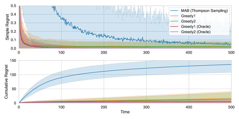
Figure 1: Simple and cumulative regret for bandit algorithms.

In this work, we present the first latent bandit model with nonlinear contextual information. We also a present an identifiability result for nonlinear ICA when the source variable differ only mean. We evaluated our results on simulated data. Our result show promise that a general use of observational data, even from noisy data could be effectively put to use for bandit algorihtms. For future work we plan to expand the bandit framework for pure exploration setting and give theoretical guarantees for regret minimization. We are also interested in the missspecified LVM case, in which the latent variable model does not generalize well to the new observation. An interesting goal in this setting would be to use a meta-algorithm to detect model missepecification and possibly change algorithms.

Appendix A Appendix

A.1 Recovery of the indicator conditional distribution

Hyvarinen and Morioka [2016] give an argument for recovering the conditional probability of the patient/instance indicator (in their case, “segment”), stated here as Lemma 1.

Lemma 1.

For a given observation $\mathbf{x}$ the likelihood of belonging to the patient $q$ in Equation 2 would converge in the limit to the following:

$$p\left(C_{q}=\xi\mid\mathbf{x}\right)=\frac{p_{\xi}\left(\mathbf{x}\right)p\left(C_{q}=\xi\right)}{\sum_{j=1}^{Q}p_{j}\left(\mathbf{x}\right)p\left(C_{q}=j\right)},$$ (5)

where $C_{q}$ is the patient label, $p_{\xi}(\mathbf{x})=p(\mathbf{x}|C_{\xi})$ is the conditional distribution of the signal, and $p(C_{q}=\xi)$ are prior distributions for each patient. Then we have for $\mathbf{h}\left(\mathbf{x};\mathbf{\varphi}\right)$:

$$\mathbf{W}_{\xi}^{T}\mathbf{h}\left(\mathbf{x};\mathbf{\varphi}\right)+\mathbf{b}_{\xi}=\log p_{\xi}\left(\mathbf{x}\right)-\log p_{1}\left(\mathbf{x}\right)+c_{\xi},$$ (6)

here $c_{\xi}=\frac{p(C_{q}=\xi)}{p(C_{q}=1)}$ relates to the length of given patient history for each patient.

A.2 Proof of Thm 1

Proof.

According to 1 the conditional distribution of $Z$ will be normal around the true mean, with the $\log$-pdf given by:

$$\log p_{\xi}(\mathbf{z})=\sum_{i=1}^{n}\frac{(z_{i}-\mu_{\xi,i})^{2}}{\sigma^{2}},$$ (7)

where each $\mu_{\xi,i}$ denotes the true patient latent state. Using change of variables we have:

$$\log p_{\xi}(\mathbf{x})=\sum_{i=1}^{n}\frac{(f_{i}(\mathbf{x})-\mu_{\xi,i})^{2}}{\sigma^{2}}+\log|det\mathbf{J}f(\mathbf{x})|$$ (8)

Take $\xi=1$ in (8):

$$\log p_{1}(x_{1})=\sum_{i=1}^{n}\frac{(f_{i}(\mathbf{x})-\mu_{1,i})^{2}}{\sigma^{2}}+\log|det\mathbf{J}f(\mathbf{x})|$$ (9)

Using (9) for the $\log p_{1}$ term in 1:

$$\log p_{\xi}(\mathbf{x})=\sum_{i=1}^{n}\left[w_{\xi,i}h_{i}(\mathbf{x})+\frac{(f_{i}(\mathbf{x})-\mu_{1,i})^{2}}{\sigma^{2}}\right]+\log|det\mathbf{J}f(\mathbf{x})|+b_{\xi}-c_{\xi}$$ (10)

Finally, taking (10) and (8) equal for arbitrary $\xi$:

$$\sum_{i=1}^{n}\frac{(f_{i}(\mathbf{x})-\mu_{\xi,i})^{2}-(f_{i}(\mathbf{x})-\mu_{1,i})^{2}}{\sigma^{2}}=\sum_{i=1}^{n}w_{\xi,i}h_{i}(\mathbf{x})+\beta_{\xi}$$ (11)

where $\beta_{\xi}=b_{\xi}-c_{\xi}$.

Simplifying (11), we have:

$$\sum_{i=1}^{n}\frac{-2f_{i}(\mathbf{x})(\mu_{\xi,i}-\mu_{1,i})+\mu_{\xi,i}^{2}-\mu_{1,i}^{2}}{\sigma^{2}}=\sum_{i=1}^{n}w_{\xi,i}h_{i}(\mathbf{x})+\beta_{\xi}$$ (12)

∎

A.3 LVM results and experiments

Table 2: Complete LVM fitting results. $L$ layers in the MLP, $T_{o}$ time steps.

$L$	$T_{o}$	Accuracy	MCCZ Train	MCCZ Test	$R^{2}_{R}$ Train	$R^{2}_{R}$ Test
2	100	0.22	0.84	0.89	0.97	0.94
2	200	0.21	0.88	0.91	0.97	0.93
2	300	0.22	0.93	0.87	0.94	0.93
4	100	0.21	0.95	0.89	0.95	0.84
4	200	0.20	0.97	0.90	0.97	0.90
4	300	0.20	0.97	0.94	0.97	0.88

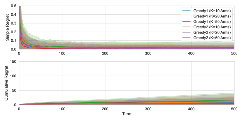
Figure 2: Simple and cumulative regret for bandit algorithms in the cases of $K=10$, $K=20$, and $K=50$ arms.

A.4 Greedy1 has constant regret

Recall that the cumulative regret, after $T$ rounds, is defined as

$$R_{T}=T\theta_{a^{*}}^{\top}\mathbf{z}-\sum_{t=1}^{T}\theta_{a_{t}}^{\top}\mathbf{z}$$

where $a^{*}$ is the optimal arm and $a_{t}$ the armed played by the algorithm at time $t$. The following Theorem follows from standard concentration results for sub-Gaussian random variables, see Theorem 3.

Theorem 2.

Let $\Delta>0$ such that $|\left(\theta_{a^{*}}-\theta_{a}\right)^{\top}\mathbf{z}|>\Delta,\forall a\neq a^{*}$ and assume $\|\theta_{a}\|_{2}=1,\forall a$. Then the expected regret of Greedy1, if the latent model is well-specified, satisfy

$$\mathbb{E}[R_{T}]\leq O(1).$$

Proof.

Greedy1 will play a sub-optimal arm $a$ if $\theta_{a}^{\top}\hat{\mathbf{z}}_{t}\geq\theta_{a^{*}}^{\top}\hat{\mathbf{z}}_{t}$ where

$$\hat{\mathbf{z}}_{t}:=\frac{1}{t}\sum_{s=1}^{t}\mathbf{z}_{s},$$

and $\mathbf{z}_{s}$ is the noisy observation made at time $s$. Hence, if for all arms we have

$$|\theta_{a}^{\top}\left(\hat{\mathbf{z}}_{t}-\mathbf{z}\right)|\leq\frac{\Delta}{2}$$

Greedy1 will play the optimal arm. Note that (Emil: Note that we are missing a $1/t$ below)

$$\left|\theta_{a}^{\top}\left(\hat{\mathbf{z}}_{t}-\mathbf{z}\right)\right|=\left|\theta_{a}^{\top}\sum_{s=1}^{t}\mathbf{\eta}_{s}\right|$$

since, $\mathbf{z}_{s}=\mathbf{z}+\mathbf{\eta}_{s}$ where each element in $\mathbf{\eta}_{s}$ is $\mathcal{N}(0,\sigma^{2})$.

Hence, using the union bound,

$$\mathbb{E}[R_{T}]\leq\overline{\Delta}\sum_{a}\sum_{t=1}^{T}P\left(\left|\theta_{a}^{\top}\sum_{s=1}^{t}\mathbf{\eta}_{s}\right|\geq\frac{\Delta}{2}\right)$$

where $\overline{\Delta}=\max_{a\neq a^{*}}\mathbf{z}^{\top}(\theta_{a^{*}}-\theta_{a})$. We now apply Theorem 3 with $w=\theta_{a}$ which yields

$$P\left(\left|\theta_{a}^{\top}\sum_{s=1}^{t}\mathbf{\eta}_{s}\right|\geq\frac{\Delta}{2}\right)\leq 2\exp\left[-\frac{t\Delta^{2}}{4\sigma^{2}}\right]$$

since $\|\theta_{a}\|=1$. Putting it together yields

$$\mathbb{E}[R_{T}]\leq K\overline{\Delta}\sum_{t=1}^{\infty}2\exp\left[-\frac{t\Delta^{2}}{4\sigma^{2}}\right]=2K\overline{\Delta}\left(\exp\left[\frac{\Delta^{2}}{4\sigma^{2}}\right]-1\right)^{-1}\leq O(1).$$

∎

Theorem 3 (General Hoeffding’s Inequality [Vershynin, 2018]).

Let $X_{1},...,X_{d}$ be independent, zero-mean, sub-Gaussian random variables and let $w\in\mathbb{R}^{d}$. Then for every $\gamma>0$

$$P\left(|\sum_{i=1}^{d}X_{i}w_{i}|\geq\gamma\right)\leq 2\exp\left[-\frac{\gamma^{2}}{Q^{2}||w||_{2}^{2}}\right]$$

with $Q^{2}$ equal to the maximum variance of any of the $X_{i}$:s.

References

- Bareinboim et al. [2015] Elias Bareinboim, Andrew Forney, and Judea Pearl. Bandits with unobserved confounders: A causal approach. Advances in Neural Information Processing Systems, 28, 2015.
- Comon [1994] Pierre Comon. Independent component analysis, a new concept? Signal processing, 36(3):287–314, 1994.
- Gittins [1979] John C Gittins. Bandit processes and dynamic allocation indices. Journal of the Royal Statistical Society Series B: Statistical Methodology, 41(2):148–164, 1979.
- Håkansson et al. [2020] Samuel Håkansson, Viktor Lindblom, Omer Gottesman, and Fredrik D Johansson. Learning to search efficiently for causally near-optimal treatments. Advances in Neural Information Processing Systems, 33:1333–1344, 2020.
- Hong et al. [2020] Joey Hong, Branislav Kveton, Manzil Zaheer, Yinlam Chow, Amr Ahmed, and Craig Boutilier. Latent bandits revisited. Advances in Neural Information Processing Systems, 33:13423–13433, 2020.