Engineering high Chern number insulators
Abstract
The concept of Chern insulators is one of the most important buliding block of topological physics, enabling the quantum Hall effect without external magnetic fields. The construction of Chern insulators has been typically through an guess-and-confirm approach, which can be inefficient and unpredictable. In this paper, we introduce a systematic method to directly construct two-dimensional Chern insulators that can provide any nontrivial Chern number. Our method is built upon the one-dimensional Rice-Mele model, which is well known for its adjustable polarization properties, providing a reliable framework for manipulation. By extending this model into two dimensions, we are able to engineer lattice structures that demonstrate predetermined topological quantities effectively. This research not only contributes the development of Chern insulators but also paves the way for designing a variety of lattice structures with significant topological implications, potentially impacting quantum computing and materials science. With this approach, we are to shed light on the pathways for designing more complex and functional topological phases in synthetic materials.
I Introduction
Topological physics, which has been one of the most hot topics in condensed matter physics in the last decade, historically began with quantum Hall effect based on the electronic Landau levels v. Klitzing et al. (1980). Haldane predicted quantum Hall effect without external magnetic field on a graphene, so called a Chern insulator Haldane (1988), which attracted huge attention after topological insulators were found Kane and Mele (2005); Bernevig and Zhang (2006); Hasan and Kane (2010). Although Haldane’s quantum Hall effect on a graphene is much weaker than was predicted, it has its significance in understanding topological materials. It is the very basic building block for the theory of band topology. Differently from the quantum Hall effect under external magnetic field, the Haldane’s original model supports Chern number only or 0. Chern insulators with Chern number larger than one will be very useful for quantum technology such as quantum computing based on electronics, photonics, and so on. Graphene-like hexagonal lattice with long range hoppings was theoretically proposed for a high Chern number insulator Sticlet and Piéchon (2013). Recently, multilayer quantum anomalous Hall system was also proposed and experimentally realized for high Chern number insulators with various Chern numbers et. al. (2020a, b); Wang and Li (2021); Wenxuan Zhu and Pan (2022).
Typically, to make a new Chern insulator in a tight-binding model, one has to guess the bulk structure of a system and the complex hopping strengths to find out the Chern number only after system-dependent Berry flux integration. In this work, we propose a systematic procedure to build Chern insulators with any Chern number. The procedure is based on the Rice-Mele(RM) model Rice and Mele (1982), a generalized version of the Su-Schrieffer-Heeger(SSH) model W. P. Su and Heeger (1979).
II Theoretical concept
Figure 1(a) represents RM model with unit cell size , whose Hamiltonian is
| (1) |
Here, represents the cell vectors with and being the cell size. The value of represents the on-site energy difference between and sites, and are inter- and intra-cell hopping constants, is the creation operator on the site () in the unit cell at , and represents hermitian conjugate. With Fourier transformation, , together with positions of two sites within a unit cell, and , the Hamiltonian can be rewritten as a Bloch form of with
| (2) |
where is the reciprocal lattice vector, and s are the Pauli matrices (see Appendix for details). Differently from the SSH model, the Zak phase, Zak (1989), can have all the values from 0 to up to multiple of phase ambiguity, owing to the energy difference between and sites. Here, is the eigenvector of . We calculate the Zak phase numerically by obtaining and using
| (3) |
instead of its differential form, where, Resta (2000). Eq. (3) does not need the differentiability of in terms of . One has to keep in mind that with being the position operator that has two values, or .
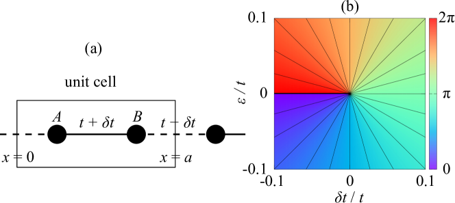
Figure 1(b) shows calculated numerically. It demonstrates that for small and compared to , where means the argument of a complex number . A pair of parameters can always be found for any given as
| (4) |
with an arbitrary parameter . The condition , that is required for the approximation of Eq. (4), is in fact not necessary for the topological implication since what only matters is the phase winding around the sigular point in Fig. 1(b). The extra multiples of two are for the simplicity of the formulas in the following part. Rice-Mele model is a one-dimensional (1D) system that can modulate with two control parameters, and . For example, positive with zero yields , so that the expectation value of position operator becomes ; it represents the middle of the strong bond in Fig. 1(a). This case corresponds to the trivial topological phase with no edge states. In many literatures, trivial phase corresponds to . It, however, is only a matter of convention of setting the positions of two subsites and while for trivial topological phase can be achieved from our formalism by setting and . The reason of choice of our convention is to confine two sites within a unit cell.
On the other hand, a Chern insulator is a two-dimensional (2D) system with along one axis winding the two-torus of the first Brillouin zone with integral number of times. For a 2D system in a rectangular coordinate system, the matrix representation of a Bloch Hamiltonian can be written as . Let us assume a rectangular lattice system with two orthogonal unit vectors of and , so that and ). For a fixed , one can calculate along the axis, . If this value varies by as changes by , the system is topologically classified to have Chern number of Hasan and Kane (2010).
III results and discussion
We propose a procedure to construct a 2D Chern insulator using 1D RM model by building up change of along an additional dimension of Bloch momentum space; A 2D system satisfying makes change by as changes by . Using Eq. (4), and for a given can be set to be
and hence Eq. (2), with , can be extended to 2D Hamiltonian with Chern number such that , where , and
| (5) |
So is built, this Hamiltonian has varying by the amount of as changes by ; a Chern insulator with a Chern number of .
In order to find out the corresponding real space representation of this , one can use 2D inverse Fourier transformation of the creation operator,
| (6) |
where and with and being the sizes of the unit cells along the and axis and . With and , can be transformed back into real space (see Appendix B for details) as
| (7) |
Figure 2(a) shows the hopping configuration corresponding to such a system with .
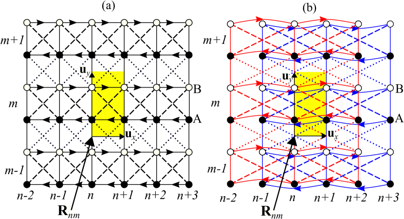
The solid, dashed and dotted lines without arrows represent bondings with real hopping constants of , and , respectively. Solid and empty circles repesent and sites. The yellow rectangle is a unit cell with and as the unit vectors. The lines with arrows represent hopping constants along the direction of the arrow and along the opposite direction. The convention of hopping direction is that the coefficient of corresponds to the hopping constant from the to the site. It implies staggered magnetic flux perpendicular to the plane which cancels out within each unit cell similar to the Haldane’s Chern insulator. It is noteworthy that the on-site energy difference between two subsites is zero even though it is built from the RM model that has non-zero on-site energy difference. Instead, the imaginary hopping constants along the and sites have opposite signs. The inter-site next nearest hopping constants also have two opposite signs within a unit cell.

We have calculated the chiral edge states with open boundary conditions along the and axis, respectively. Figure 3(a) and (c) show the band structures for the case with a pair of edges along the and axis respectively for . The value of that decides the gap size is set to be . The number of unit cells between edges are chosen to be 60. The number of gapless chiral edge band lines is 2 since there are two edges.
Figure 2(b) shows the configuration for . For a general case of , the -th site is connected to the -th site by hopping along the axis so that only -th sites are connected to -th sites with . In such a manner, the system is partitioned into decoupled subsystems. In Fig. 2(b), two subsystems are colored distinctly as red and blue. Furthermore, each decoupled system is identical to the system in terms of the hopping graph. With an open boundary condition, since the structure consists of copies of a Chern number one system, it should show gapless boundary band lines for each edge. This means that its Chern number is as supposed. Figure 3(b) and (d) show the band structures for open boundary condition with a pair of edges along the and axis respectively, for . Each of the two band lines corresponding to the edge states on two edges in Fig. 3(d) has three-fold degeneracy.
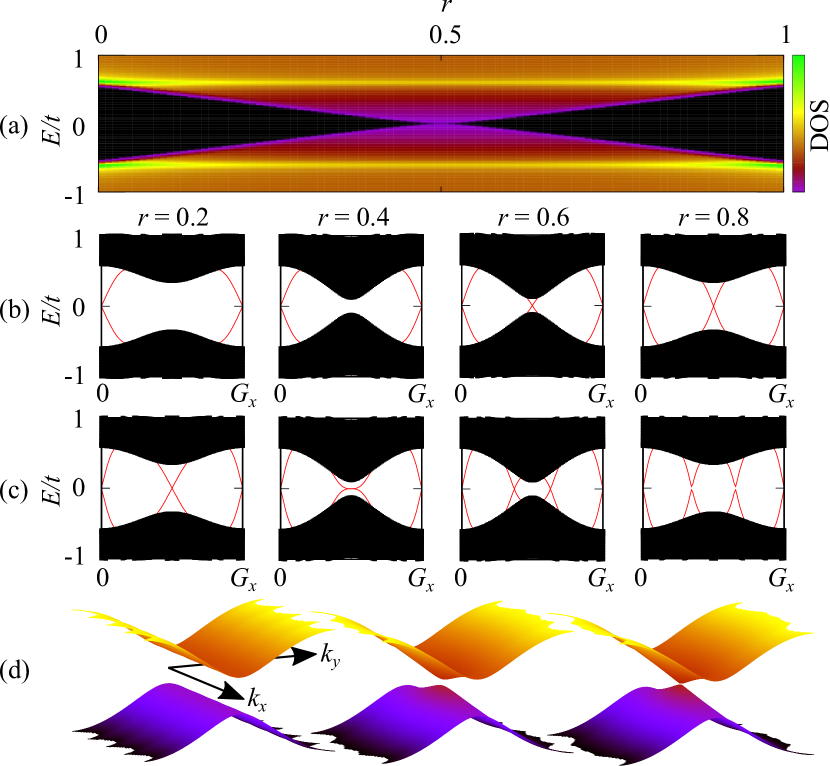
One might say that this result is trivial since the constructed high- Chern insulator is simply an overlap of copies of partially translated systems with . A nontrivial one, however, can further be constructed by mixing Hamiltonians with distinct Chern numbers. For example, the Hamiltonian that mixes and is
where is the mixing ratio. If the Hamiltonian becomes one with while if it becomes one with . Therefore, as varies from 0 to 1, the Chern number of must undergo at least one topological phase transition. At the topological transition, the bulk band gap must be closed. Figure 4(a) shows the bulk density of state (DOS) as a function of demonstrating gap closing at ; for and for . Figure 4(b) shows how the number of gapless band lines increases. Further numerical calculations confirm that the change of DOS as a funtion of the mixing ratio from to with is identical to the case from to . Figure 4(c) shows the discrete change of number of gap closing band lines from 4 to 6 as changes; makes a transition from 2 to 3 at . Figure 4(d) shows the 2D band structure for the unmixed Chern insulator with (left), for a mixed one between and at the transition point which closes gap making a Dirac cone (right), and for a general mixed one with Chern number two that shows quadratic dispersion at the zone boundary (middle). This demonstrates that by mixing different unmixed Hamiltonians, , with different values in a various way, nontrivial high Chern number insulators can be constructed on demand.
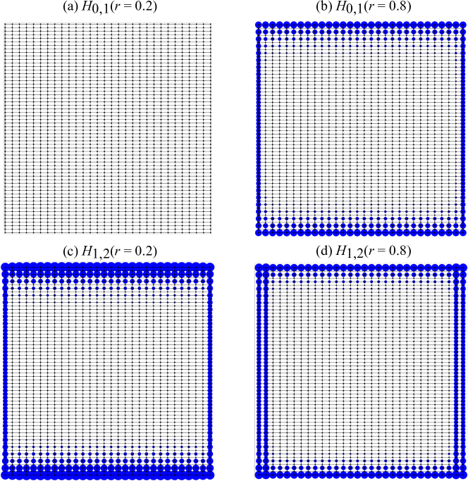
We further calculate local density of states (ldos) at with energy width of for isolated systems of size unit cells with an open boundary condition by varying the value of for and to demonstrate the emergence of chiral edge states. Figure 5 shows zero-energy ldos showing gap state density for (a) , (b) , (c) , and (d) . It demonstrates that the chiral edge states emerge once becomes larger than 0.5 in the case with [Figs. 5(a, b)]. Figures 5(b, c) have Chern number of one. Figure 5(d), that corresponds to Chern number two, shows that the edge state density covers two rows on each edge along the axis, differently from (b) and (c) where it covers only one row. Although not being a general manefestation of Chern number, it can be used for a signature of topological phase transition for this specific system if tested experimentally in the future.
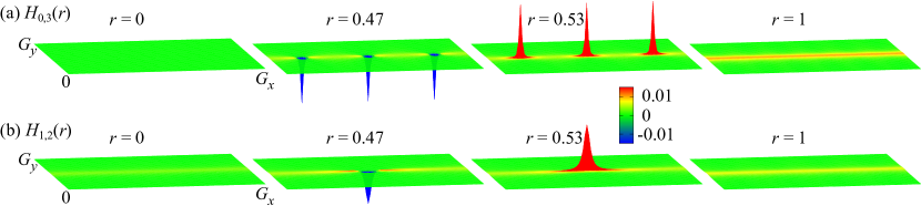
In order to further confirm the Chern number, we calculate Berry flux within the first Brillouin zone across the phase transition. Figure 6(a) and (b) shows the Berry flux for systems with and for different values of . Both cases undergo phase transition at . For , Chern number changes directly from to at . The second and third plots are Berry flux right before and after phase transtion with Chern numbers, and . The integration of Berry flux over the Brillouin zone divided by is the Chern number. For the case before the phase transition with , integration of the dispersed positive Berry flux (yellow) exactly cancels out with that of the three localized spots of negative Berry flux (blue) to make the Chern number zero. On the other hand, for the case after the phase transition with , the localized spots of Berry flux becomes singular when , changing their sign of flux to plus making the Chern number three. For , the story is similar with phase transition from Chern number one to two through one singular spot of Berry flux. We confirm that singular points of Berry flux correspond to gap closing points.
Lastly, we would like to mention briefly about experimental realization and future plans. As for the experimental realization, due to its relatively complicated nature of hopping structures it might be challenging in solid state systems. However, complicated hopping structures have been widely achieved recently in the fields such as optics and electric circuits. The next nearest neighbor and long-range hopping can be implemented in photonic systems such as an array of coupled optical-ring resonators and coupled-resonator optical waveguides, which consist of site resonators and link resonators M. Hafezi and Taylor (2013); Sunil Mittal and Hafezi (2016); Daniel Leykam and Chong (2018); JungYun Han and Leykam (2019). In a synthetic dimension, long-range hopping can also be implemented by utilizing frequency modes in two coupled ring resonators Kai Wang and Fan (2021). Asymmetric long-range hopping between resonant elements in a photonic arrangement have been achieved in active optical platforms Yuzhou G. N. Liu and Khajavikhan (2021) and complex hopping between neighboring lattice sites have been realized in electronic circuit layouts Jia Ningyuan and Simon (2015); Xiang Ni and Alù (2020); Lingling Song and Yan (2022). Our future work will include investigation of dynamical responses of topological edges states to varying Chern number by tuning the hopping parameters of these systems. It is also important to note that the experimental realization of high Chern number insulators are mostly multilayered systems et. al. (2020a, b); Wang and Li (2021); Wenxuan Zhu and Pan (2022). They consist of layers each of which has Chern number one while multilayers make copies of each layer introducing high Chern number. Such mechanism is analogous to our structure; our systems consist of laterally shifted copies of Chern number one systems.
IV Conclusion
In conclusion, we propose a systematic method to construct a two-dimensional lattice structure with proper hopping parameters that can give an arbitrary Chern number, based on extended 1D Rice-Mele model. With constructed structures, we successfully demonstrate topological phase transitions between different Chern numbers by modulating hopping parameters. We also demonstrate the emergence of topological chiral edge states across the phase transition. Generalization of our method to different lattice structures such as hexagonal lattice as well as extension to higher dimensions for higher-order topological insulators shall be of interest for future projects.
V acknowledgements
This work was supported by the National Research Foundation of Korea(NRF) grant funded by the Korea government(MSIT) (No. RS-2023-00278511), by the Pukyong National University Research Fund in (No.202303660001), by Korea Institute for Advanced Study (KIAS), and by the Institute for Basic Science in Korea (No. IBS-R024-D1).
VI references
References
- v. Klitzing et al. (1980) K. v. Klitzing, G. Dorda, and M. Pepper, Phys. Rev. Lett. 45, 494 (1980).
- Haldane (1988) F. D. M. Haldane, Phys. Rev. Lett. 61, 2015 (1988).
- Kane and Mele (2005) C. L. Kane and E. J. Mele, Phys. Rev. Lett. 95, 226801 (2005).
- Bernevig and Zhang (2006) B. A. Bernevig and S.-C. Zhang, Phys. Rev. Lett. 96, 106802 (2006).
- Hasan and Kane (2010) M. Z. Hasan and C. L. Kane, Rev. Mod. Phys. 82, 3045 (2010).
- Sticlet and Piéchon (2013) D. Sticlet and F. Piéchon, Phys. Rev. B 87, 115402 (2013).
- et. al. (2020a) Y.-F. Z. et. al., Nature 588, 419 (2020a).
- et. al. (2020b) J. G. et. al., Natl. Sci. Rev. 7, 1280 (2020b).
- Wang and Li (2021) Y.-X. Wang and F. Li, Phys. Rev. B 104, 035202 (2021).
- Wenxuan Zhu and Pan (2022) H. B. L. L. Wenxuan Zhu, Cheng Song and F. Pan, Phys. Rev. B 105, 155122 (2022).
- Rice and Mele (1982) M. J. Rice and E. J. Mele, Phys. Rev. Lett. 49, 1455 (1982).
- W. P. Su and Heeger (1979) J. R. S. W. P. Su and A. J. Heeger, Phys. Rev. Lett. 42, 1698 (1979).
- Zak (1989) J. Zak, Phys. Rev. Lett. 62, 2747 (1989).
- Resta (2000) R. Resta, J. Phys.:Condens. Matter 12, R107 (2000).
- M. Hafezi and Taylor (2013) J. F. A. M. M. Hafezi, S. Mittal and J. M. Taylor, Nature Photonics 7, 1001 (2013).
- Sunil Mittal and Hafezi (2016) J. F. A. V. Sunil Mittal, Sriram Ganeshan and M. Hafezi, Nature Photonics 10, 180 (2016).
- Daniel Leykam and Chong (2018) M. H. Daniel Leykam, S. Mittal and Y. D. Chong, Phys. Rev. Lett. 121, 023901 (2018).
- JungYun Han and Leykam (2019) C. G. JungYun Han and D. Leykam, Phys. Rev. B 99, 224201 (2019).
- Kai Wang and Fan (2021) C. C. W. Kai Wang, Avik Dutt and S. Fan, Nature 598, 59 (2021).
- Yuzhou G. N. Liu and Khajavikhan (2021) M. P. D. N. C. Yuzhou G. N. Liu, Pawel S. Jung and M. Khajavikhan, Nature Physics 17, 704 (2021).
- Jia Ningyuan and Simon (2015) A. S. D. S. Jia Ningyuan, Clai Owens and J. Simon, Phys. Rev. X 5, 021031 (2015).
- Xiang Ni and Alù (2020) A. B. K. Xiang Ni, Zhicheng Xiao and A. Alù, Phys. Rev. Applied 13, 064031 (2020).
- Lingling Song and Yan (2022) Y. C. Lingling Song, Huanhuan Yang and P. Yan, Nature Comm. 13, 5601 (2022).
Appendix A Fourier Transformation
As in Eq. (1), the Hamiltonian of a RM model is
| (8) |
With Fourier transformation, , each term can be transformed into -space. The term of is transformed as
| (9) |
The term, is transformed similarly as
| (10) |
The term, is transformed as
With and , it becomes
| (11) |
The term, is transformed as
With and , it becomes
| (12) |
Summing up terms from Eqs. (9, 10, 11, 12), Eq. (8) can be represented in -space as with
| (13) |
where and s are Pauli matrices.
Appendix B Inverse Fourier Transformation
From Eq. (5), the hamiltonian with Chern number in the -space representation consists of three terms as
| (14a) | ||||
| (14b) | ||||
| (14c) | ||||
Each term can be transformed into the representation of real space using Eq. (6). The first term, Eq. (14a), transforms as
| (15) |
Here, is used. The sencond term, Eq. (14b), transforms as
| (16) |
The third term, Eq. (14c) transforms as
| (17) |
Summing up terms from Eqs. (15, 16, 17), the Hamiltonian can be written in the real space as
| (18) |