Probabilistic Parameter Estimators and Calibration Metrics for Pose Estimation from Image Features

Abstract

This paper addresses the challenge of probabilistic parameter estimation given measurement uncertainty in real-time. We provide a general formulation and apply this to pose estimation for an autonomous visual landing system. We present three probabilistic parameter estimators: a least-squares sampling approach, a linear approximation method, and a probabilistic programming estimator. To evaluate these estimators, we introduce novel closed-form expressions for measuring calibration and sharpness specifically for multivariate normal distributions. Our experimental study compares the three estimators under various noise conditions. We demonstrate that the linear approximation estimator can produce sharp and well-calibrated pose predictions significantly faster than the other methods but may yield overconfident predictions in certain scenarios. Additionally, we demonstrate that these estimators can be integrated with a Kalman filter for continuous pose estimation during a runway approach where we observe a 50% improvement in sharpness while maintaining marginal calibration. This work contributes to the integration of data-driven computer vision models into complex safety-critical aircraft systems and provides a foundation for developing rigorous certification guidelines for such systems.

I Introduction

Automation in aviation has recently gained technological advancements based on data-driven models applied to vision, decision-making, planning, and human interaction. A direct “proof of correctness” or “learning assurance” for such models currently seems far away, making practitioners and regulators resort to other approaches [1, 2, 3, 4, 5]. These approaches may include test set validation [6], out-of-distribution detection [7], causal models [8, 9, 10], mechanistic interpretability [11, 12, 13], adversarial robustness [14], uncertainty estimation [15, 16, 17], and calibration [18, 19, 20].

In this work, we focus on the principled processing and validation of model output uncertainty. First, we consider a general setting for probabilistic parameter estimation from uncertain measurements. Then, we consider the pose estimation problem arising as part of an autonomous visual landing system. We assume that the system relies on a data-driven computer vision algorithm that finds the exact projection location of runway corners in the image, and has known reference coordinates. Further, we assume the model dynamically produces a quantification of uncertainty in its predictions.

This paper makes the following contributions:

1. Three formulations for general uncertainty-aware parameter estimation, and their specific formulation for the pose estimation problem;

2. A novel closed-form expression for measuring calibration and sharpness for multivariate normal distributions; and

3. An experimental study comparing the three estimators for pose estimation using calibration and sharpness metrics.

The paper is organized as follows. Section II provides some necessary background and notation. Section III first proposes three estimators for probabilistic parameter estimation based on (i) repeated noise sampling and least-squares minimization, (ii) a linear approximation, and (iii) a Bayesian approach solved using Markov Chain Monte Carlo, and then discusses integrating the proposed estimators into a Kalman filter.

Section IV introduces techniques to evaluate the quality of multivariate probabilistic predictions through (i) calibration and (ii) sharpness. In particular, we propose closed-form expressions for efficiently computing calibration and sharpness for multivariate normal distributions given ground truth observations, which allow us to compare the efficacy of the proposed estimators.

Section V presents experimental results for all three estimators applied to an aircraft pose estimation problem during a runway approach under different noise conditions. We find that the linear approximation estimator typically constructs sharp and calibrated predictions two orders of magnitude faster than the other estimators. However, we also find that it produces overconfident predictions in particular scenarios. We further demonstrate integration of the estimators with a Kalman filter for a single approach, which leads to a $2\times$ improvement in sharpness, while maintaining marginal calibration.

Overall, this work aims to improve understanding of how to best integrate data-driven computer vision models into complex safety-critical aircraft, and further provide a foundation upon which rigorous certification guidelines for such systems can be built. Code supporting this work is available online.

II Preliminaries

We briefly introduce necessary notation and phrase pose estimation as a general parameter estimation problem. This section reviews least squares estimation given measurement uncertainty. We then discuss how to represent measurement and pose uncertainty, and how to evaluate whether a series of predictions is (i) probabilistically “correct” (calibrated) and (ii) precise (sharp).

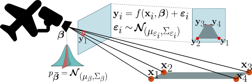
Figure 1: Known world points $\mathbf{x}_{i}$ are projected onto a camera at $\bm{\upbeta}$, where they are measured as $\mathbf{y}_{i}$ under the influence of noise. We wish to determine $\bm{\upbeta}$ or a distribution over $\bm{\upbeta}$.

II-A Camera Model for Point Projections

Consider the pose estimation problem for an aircraft approaching a runway approach using image features with known corresponding world points. We assume a (pinhole) camera located on the aircraft, positioned such that the entire runway is in view of the camera lens. Figure 1 presents an overview.

Let the camera projection function $\mathbf{y}=f(\mathbf{x},\bm{\upbeta})$ map a world point $\mathbf{x}=[x_{[\text{alongtrack}]},x_{[\text{crosstrack}]},x_{[\text{altitude}]}]$ to an image projection $\mathbf{y}=[y_{[\text{right}]},y_{[\text{up}]}]$ given a camera position $\bm{\upbeta}=[\beta_{[\text{alongtrack}]},\beta_{[\text{crosstrack}]},\beta_{[\text{altitude}]}]$

Consider now a focal-point-centric coordinate system rotated such that the $x$-axis goes from the focal point through the center of the camera projection plane towards the world points, and the $y$- and $z$-axes are parallel to the projection plane’s edges. If we write the location of the world points in this coordinate system as $[x^{\prime},y^{\prime},z^{\prime}]$, we can compute the camera projection coordinate simply as

$$\mathbf{y}=\lambda_{\text{focal length}}\cdot\frac{1}{x^{\prime}}\begin{bmatrix}y^{\prime}\\ z^{\prime}\end{bmatrix}.$$ (1)

We will use the notation

$$\mathbf{y}_{i}=\begin{bmatrix}\left(y_{i}\right)_{[1]}\\ \left(y_{i}\right)_{[2]}\end{bmatrix},\quad i\in\mathcal{I}$$ (2)

to denote the first and second components of the $i$-th observation $\mathbf{y}_{i}$, with $\mathcal{I}=\left\{1,2,3,4\right\}$ for the four runway corners. We denote random variables with a hat and write

$${\bar{\xi}}^{(k)}\sim p_{\bar{\xi}},$$ (3)

to denote the $k$-th sample of the random variable $\bar{\xi}$ that follows the distribution $p_{\bar{\xi}}$. Upright bold variables such as $\mathbf{y}$ denote vectors, and matrices are uppercase such as $\Sigma$.

II-B Pose-from-N-Points (PNP)

To solve the PNP problem in its basic form, it is now sufficient to solve the nonlinear least-squares problem

$$\bm{\upbeta}=\arg\min\limits_{\bm{\upbeta}}\sum_{i}{d\left(\mathbf{y}_{i},f\left(\mathbf{x}_{i},\bm{\upbeta}\right)\right)}^{2}$$ (4)

where $d(\cdot,\cdot)$ is the Euclidean distance. For other problem settings, $d$ and $f$ can take a variety of forms. For example, if $f$ computes sidelines angles other geometric features, such as sideline angles, an appropriate distance functions may be chosen. We also point out that for point projections, due to the nonlinearity of the projection function $f(\cdot,\cdot)$, this problem is numerically challenging to solve. In particular, for low altitudes, the inverse problem becomes very sensitive to small changes in the projection. Nonetheless, for approach angles of at least $\qty{1}{}$ above ground, the PNP problem can typically be solved using, e.g., the Newton-Raphson, Levenberg-Marquardt, or trust region algorithms.

II-C Least-squares Under Measurement Noise

If weights $w_{i}$ for each observation are available, we may rewrite Eq. 4 as

$$\bm{\upbeta}=\arg\min\limits_{\bm{\upbeta}}\sum_{i}w_{i}\cdot{d\left(\mathbf{y}_{i},f\left(\mathbf{x}_{i},\bm{\upbeta}\right)\right)}^{2}$$ (5)

where weights are typically chosen as the inverse variance of each observation, i.e., $w_{i}=1/{\sigma_{y}^{2}}_{i}$ [21]. For noise that is correlated across observations, we can instead concatenate all components into a single vector

$${\mathbf{r}}(\bm{\upbeta})=\begin{bmatrix}d\left(\mathbf{y}_{1},f\left(\mathbf{x}_{1},\bm{\upbeta}\right)\right)\\ d\left(\mathbf{y}_{2},f\left(\mathbf{x}_{2},\bm{\upbeta}\right)\right)\\ \vdots\end{bmatrix}$$ (6)

where each component $d(\cdot,\cdot)$ may be further expanded if it has multiple components (such as component-wise distances). Then we can rewrite Eq. 5 as

$$\bm{\upbeta}=\arg\min\limits_{\bm{\upbeta}}{\mathbf{r}(\bm{\upbeta})}^{\top}W\mathbf{r}(\bm{\upbeta})$$ (7)

where $W$ denotes the weight matrix which can be chosen as the inverse variance-covariance matrix of the observation noise, e.g. $\Sigma_{\mathbf{y}}^{-1}$ for the case of Gaussian noise [21].

Notice that we can also rewrite Eq. 7 as

$$\bm{\upbeta} =\arg\min\limits_{\bm{\upbeta}}{\tilde{\mathbf{r}}}(\bm{\upbeta})^{\top}\tilde{\mathbf{r}}(\bm{\upbeta})$$ (8)

$$=\arg\min\limits_{\bm{\upbeta}}\sum_{i}{\tilde{r}}_{i}^{2}(\bm{\upbeta})$$

by LU-factorizing $W=LU$ and setting $\tilde{\mathbf{r}}=U{\mathbf{r}}$ in the general case, or $\Sigma=LU$ and $\tilde{\mathbf{r}}=L^{-\top}{\mathbf{r}}$ in the Gaussian noise case. This representation is sometimes preferable for mathematical convenience and solver interfaces.

II-D Representing Measurement and Pose Uncertainty

If our world points $\left\{\mathbf{x}_{i}\right\}_{i\in\mathcal{I}}$ and measurements $\left\{\mathbf{y}_{i}\right\}_{i\in\mathcal{I}}$ are known, we can solve the pose estimation problem as a nonlinear least squares optimization as shown above. However, our measurements $\mathbf{y}_{i}$ and world points $\mathbf{x}_{i}$ can be noisy or uncertain, and may therefore be provided through a probabilistic description, e.g., a Gaussian or other distribution, or samples drawn from a distribution.

In this scenario, our pose estimate will be a random variable $\bar{\bm{\upbeta}}$, or more precisely, $\bar{\bm{\upbeta}}\mid{\{(\bar{\mathbf{x}}_{i},\bar{\mathbf{y}}_{i})\}}_{i\in\mathcal{I}}$. We therefore need to represent the pose either (i) through samples (to which a distribution may be fitted) or (ii) directly as a (multivariate) distribution. In these cases, we write

$$\left({\bar{\bm{\upbeta}}}^{(1)},{\bar{\bm{\upbeta}}}^{(2)},\ldots\right)\overset{\text{ i.i.d.}}{\sim}p_{\bar{\bm{\upbeta}}\mid{\{(\bar{\mathbf{x}}_{i},\bar{\mathbf{y}}_{i})\}}_{i\in\mathcal{I}}}$$ (9)

with realizations $\left(\bm{\upbeta}^{(1)},\bm{\upbeta}^{(2)},\ldots\right)$, or

$$p_{\bar{\bm{\upbeta}}\mid{\{(\bar{\mathbf{x}}_{i},\bar{\mathbf{y}}_{i})\}}_{i\in\mathcal{I}}}\approx{\mathcal{N}}_{(\mu,\Sigma)},$$ (10)

respectively. Notice that due to the non-linearity in the projection in Eq. 1, the distribution $p_{\bar{\bm{\upbeta}}\mid{\{(\bar{\mathbf{x}}_{i},\bar{\mathbf{y}}_{i})\}}_{i\in\mathcal{I}}}$ will not in general be Gaussian, even for Gaussian noise in the measurements. However, we will see that approximating $p_{\bar{\bm{\upbeta}}\mid{\{(\bar{\mathbf{x}}_{i},\bar{\mathbf{y}}_{i})\}}_{i\in\mathcal{I}}}$ as a Gaussian ${\mathcal{N}}_{(\mu,\Sigma)}$ does yield good results for our problem.

II-E Calibration and Sharpness

Calibration gives us a way to quantify whether the uncertainty in a series of predictions is faithful to the distribution of prediction errors. Given a set of predicted probability distributions $p_{{\bar{\xi}}_{i}}$ and corresponding measurements $\xi_{i}$, we call the predictions (marginally) calibrated if

$$\text{Pr}\left(\bar{\xi}_{i}\leq q(p_{\bar{\xi}_{i}},\rho)\right)\approx\rho\quad\forall\rho\in(0,1),$$ (11)

where $q(p_{\bar{\xi}_{i}},\rho)$ denotes the quantile function for the random variable ${\bar{\xi}}_{i}$ evaluated at $\rho$. Notably, however, the quantile function is not defined for multivariate distributions such as $p_{\bar{\bm{\upbeta}}\mid{\{(\bar{\mathbf{x}}_{i},\bar{\mathbf{y}}_{i})\}}_{i\in\mathcal{I}}}$ in Eq. 9 and Eq. 10. We must therefore generalize Eq. 11 to remove the dependence on the quantile function and instead rely on the more general notion of prediction sets. We present such a solution in Section IV.

Further, we note that a series of predictions may be perfectly calibrated yet still be “bad” in the sense that each prediction has large uncertainty. Therefore, we must also measure sharpness, a measure of the “conciseness” of the predictions. We propose a measure of sharpness for multivariate normal distributions in Section IV-D and refer to [22] for an overview of the trade off between calibration and sharpness.

III Three Probabilistic Estimators

Given an observation function $f(\cdot,\cdot)$ and measurement tuples ${\{(\mathbf{x}_{i},\mathbf{y}_{i})\}}_{i\in\mathcal{I}}$, we have seen how to estimate the parameter $\bm{\upbeta}$, incorporating measurement uncertainties through a weighting scheme given in Section II-C. However, this process will only give us the maximum likelihood estimator for $\bm{\upbeta}$, i.e.

$$\bm{\upbeta}=\arg\max\limits_{\bm{\upbeta}}p_{\bar{\bm{\upbeta}}\mid{\{(\bar{\mathbf{x}}_{i},\bar{\mathbf{y}}_{i})\}}_{i\in\mathcal{I}}}(\bm{\upbeta}).$$ (12)

Instead, we are now interested in constructing a probabilistic description of the parameter $\bm{\upbeta}$ as a distribution or a set of samples. We propose three estimators for this task: (i) the least-squares sampling estimator, (ii) the linear approximation estimator, and (iii) the MCMC estimator. We show that although the three methods differ in mathematical rigor and runtime cost, their performance often matches closely.

III-A The LSQ Estimator via Noise Sampling

The simplest approach to constructing a sampled representation of $p_{\bar{\bm{\upbeta}}}$ is to repeatedly sample simulated noise and solve the least-squares formulation for each noise sample. To construct the $k$th pose estimate $\bm{\upbeta}^{(k)}$, we draw a noise sample $\bm{\upvarepsilon}_{i}^{(k)}$ for each corner projection $\mathbf{y}_{i}$ and solve the least squares formulations from Eq. 8 where we substitute

$$\mathbf{y}_{i}\leftarrow\mathbf{y}_{i}-\bm{\upvarepsilon}_{i}^{(k)}$$ (13)

for each $i$. Repeating this a number of times will result in a set of estimates

$$\{\bm{\upbeta}^{(k)}\}_{k\in\mathcal{K}}=\{\bm{\upbeta}^{(1)},\bm{\upbeta}^{(2)},\ldots,\bm{\upbeta}^{\left(|\mathcal{K}|\right)}\}$$ (14)

which we may optionally approximate as a distribution $p_{\bar{\bm{\upbeta}}\mid{\{(\bar{\mathbf{x}}_{i},\bar{\mathbf{y}}_{i})\}}_{i\in\mathcal{I}}}$ by fitting a multivariate normal distribution to the samples. For the pose estimation application we find that a number of samples $|\mathcal{K}|$ between 100 and 500 is typically sufficient.

Notably, the LSQ Estimator does not require us to make any assumptions about the prior distribution $p_{\bar{\bm{\upbeta}}}$ or the shape of the posterior $p_{\bar{\bm{\upbeta}}\mid{\{(\bar{\mathbf{x}}_{i},\bar{\mathbf{y}}_{i})\}}_{i\in\mathcal{I}}}$ (which is in general not a perfect Gaussian), nor does it require strong assumptions about the function $f(\cdot,\cdot)$. Indeed, even multimodal posterior distributions can be approximated with this method.

The downside of this method is that the computational cost is rather high, as the full least-squares problem has to be solved for every sample of $\bm{\upbeta}^{(k)}$. However, starting from the second sample, setting the initial guess for $\bm{\upbeta}^{(k)}$ to the solution of $\bm{\upbeta}^{(k-1)}$ can significantly reduce the runtime cost.

III-B Linear Approximation Estimator

The LSQ Estimator suffers from high computational cost, since it has to solve the least squares problem many times. However, if we approximate the projection function $f\left(\mathbf{x},\bm{\upbeta}\right)$ as a linear function around some sample $\bm{\upbeta}^{(1)}$, and assume the noise to be Gaussian, we can construct $p_{\bar{\bm{\upbeta}}}$ in a single step by directly propagating the uncertainty in the observations $\mathbf{y}$. We call this estimator the Linear Approximation Estimator.

Let $J_{ij}=\frac{\partial f_{i}\left(\mathbf{x},\bm{\upbeta}\right)}{\partial\beta_{j}}$ be the Jacobian of our projection function. We can relate changes in $\bm{\upbeta}$ and $\mathbf{r}$ or $\widetilde{\mathbf{r}}$ as

$$J\Delta\bm{\upbeta} =-\Delta\widetilde{\mathbf{r}},$$ (15)

$$\Rightarrow\left(J^{\top}WJ\right)\Delta\bm{\upbeta} =-J^{\top}W\Delta\mathbf{r}.$$

With $\mathbf{r}_{i}=\mathbf{y}_{i}-f\left(\mathbf{x},\bm{\upbeta}\right)$ and $\mathbf{y}_{i}=f\left(\mathbf{x}_{i},\bm{\upbeta}\right)+\bm{\upvarepsilon}_{i}$ we can model $\Delta\mathbf{r}=-\bm{\upvarepsilon}$ and therefore treat $\Delta\bm{\upbeta}$ as a random variable $\mkern 4.0mu\overline{\mkern-4.0mu\Delta\bm{\upbeta}\mkern-4.0mu}\mkern 4.0mu$ with distribution

$$p_{\mkern 4.0mu\overline{\mkern-4.0mu\Delta\bm{\upbeta}\mkern-4.0mu}\mkern 4.0mu}=\left(J^{\top}WJ\right)^{-1}J^{\top}W{p_{\bar{\bm{\upvarepsilon}}}}_{i}.$$ (16)

Using this insight, we can now construct our parameter estimate $p_{\bar{\bm{\upbeta}}}$ as follows. We first estimate $\mu_{\bm{\upbeta}}$ by solving Eq. 8 once, without any noise perturbation. Then, we compute

$$p_{\bar{\bm{\upbeta}}} =\mu_{\bm{\upbeta}}+p_{\mkern 4.0mu\overline{\mkern-4.0mu\Delta\bm{\upbeta}\mkern-4.0mu}\mkern 4.0mu}$$ (17)

$$=\mu_{\bm{\upbeta}}+\left(J^{\top}WJ\right)^{-1}J^{\top}Wp_{\bar{\bm{\upvarepsilon}}}$$

which yields the desired result. For example, if $p_{\bar{\bm{\upvarepsilon}}}={\mathcal{N}}_{\left(\mathbf{0},\Sigma_{\bm{\upvarepsilon}}\right)}$ and $W=\Sigma_{\bm{\upvarepsilon}}^{-1}$ then

$$p_{\bar{\bm{\upbeta}}}={\mathcal{N}}_{\left(\mu_{\bm{\upbeta}},\Sigma_{\bm{\upbeta}}\right)}$$ (18)

with

$$\mu_{\bm{\upbeta}}=\arg\min\limits_{\bm{\upbeta}}{\mathbf{r}(\bm{\upbeta})}^{\top}\mathbf{r}(\bm{\upbeta})$$ (19)

$$\Sigma_{\bm{\upbeta}}=\left(J^{\top}\Sigma_{\bm{\upvarepsilon}}^{-1}J\right)^{-1}J^{\top}\Sigma_{\bm{\upvarepsilon}}^{-1}J\left(J^{\top}\Sigma_{\bm{\upvarepsilon}}^{-1}J\right)^{-1}.$$ (20)

Further, if $J$ is square and invertible then $\Sigma_{\bm{\upbeta}}$ reduces to

$$\Sigma_{\bm{\upbeta}}=J^{-1}\Sigma_{\bm{\upvarepsilon}}\left(J^{\top}\right)^{-1}.$$ (21)

Finally, we may replace $p_{\bar{\bm{\upvarepsilon}}}$ in Eq. 17 with $\left(p_{\bar{\mathbf{y}}}-f\left(\mathbf{x},\theta^{\text{est}}\right)\right)$ to slightly relax the assumption that $\mathbf{y}_{i}=f\left(\mathbf{x}_{i},\bm{\upbeta}\right)+\bm{\upvarepsilon}_{i}$, which can yield more robust results.

The Linear Approximation Estimator is highly efficient, only requiring to solve the least squares problem once and compute the Jacobian of $f$ one additional time. This property makes it more suitable for real-time systems such as a visual positioning system. However, in cases where the assumption of Gaussian noise does not hold (see e.g. Section V-C), or if the function is highly nonlinear, the estimator may produce poor results.

III-C MCMC Estimator

The previous two approaches have relied on a least-squares formulation of the problem, carefully constructing a weighting scheme to incorporate uncertainties correctly. Now, we present an approach based on a Bayesian formulation that can create samples $\bm{\upbeta}^{(k)}$ directly using probabilistic programming.

Our formulation is as follows. We choose a weakly informative prior $p_{\bar{\bm{\upbeta}}}$ as a diagonal multivariate normal distribution such that our entire operational domain is contained within one standard deviation of the prior. Of course, if a better prior is available it may be chosen instead. We further recall that we assume we have a model of the observation noise ${p_{\bm{\upvarepsilon}}}_{i}$ (which is now not constrained to any particular family of distribution), provided by our sensor for every sample. Then our Bayesian formulation is simply

$$\bar{\bm{\upbeta}} \sim p_{\bar{\bm{\upbeta}}}$$ (22)

$${\bar{\mathbf{y}}}_{i} \sim f\left(\mathbf{x}_{i},\bm{\upbeta}\right)+{p_{\bar{\bm{\upvarepsilon}}_{i}}}$$

which can be directly solved using Markov Chain Monte Carlo [23, 24], yielding samples $\left(\bm{\upbeta}^{(1)},\bm{\upbeta}^{(2)},\ldots\right)$.

This formulation is remarkably simple, necessitating no further thoughts about how to integrate the knowledge of uncertainties into any kind of weighting scheme, how to set up the least squares problem, or assumptions about the distributions of inputs or outputs. Further, this formulation can indeed be more computationally efficient than the noise sampling approach from Section III-A (see e.g. Table I) and can represent arbitrary distribution shapes just like the LSQ Estimator.

III-D Integrating Probabilistic Estimators Into a Kalman Filter Framework

Finally, we demonstrate how we can integrate the proposed probabilistic parameter estimators into a Kalman filter framework. Recall the Kalman filter equations (without inputs) given by

$$\mathbf{x}^{[t+1]} =A\mathbf{x}^{[t]}+\mathbf{w}^{[t]}$$ (23)

$$\mathbf{y}^{[t+1]} =C\mathbf{x}^{[t+1]}+\mathbf{v}^{[t+1]}$$

with process noise $\mathbb{E}\left[\mathbf{w}^{[t^{\prime}]}{\mathbf{w}^{[t]}}^{\top}\right]=\delta_{t^{\prime}t}Q^{[t]}$ and measurement noise $\mathbb{E}\left[\mathbf{v}^{[t^{\prime}]}{\mathbf{v}^{[t]}}^{\top}\right]=\delta_{t^{\prime}t}R^{[t]}$, i.e., Gaussian noise uncorrelated in time with covariances $Q^{[t]}$ and $R^{[t]}$ [25].

Often it is difficult to choose $R^{[t]}$ dynamically for each time step, and instead a single fixed $R$ is chosen for all time steps. Using one of the proposed estimators, however, we can dynamically compute $\mathbf{y}^{[t]}$ and $R^{[t]}$ for each time step. Consider the probabilistic parameter $\bar{\bm{\upbeta}}^{[t]}$ to represent our measurements $\mathbf{y}^{[t]}$ at time step $t$, with

$$p_{\bar{\bm{\upbeta}}^{[t]}\mid{\{(\bar{\mathbf{x}}^{[t]}_{i},\bar{\mathbf{y}}^{[t]}_{i})\}}_{i\in\mathcal{I}}}\approx{\mathcal{N}}_{(\mu^{[t]},\Sigma^{[t]})}.$$ (24)

Then, for each time step, we can set

$$\mathbf{y}^{[t]} \leftarrow\bm{\upmu}^{[t]}$$ (25)

$$R^{[t]} \leftarrow\Sigma^{[t]}.$$

Notice how this formulation differs from typical nonlinear Kalman filter formulations such as the Extended Kalman filter [25, 26]. Our measurement uncertainty is not restricted to relations $\mathbf{y}=h(\mathbf{x})+\mathbf{w}$ for some known $h(\mathbf{x})$, but instead may arise without modeling $h(\mathbf{x})$, such as measured image features with predictive uncertainty perceived from state $\mathbf{x}$.

One important additional consideration is that the Kalman filter assumes noise uncorrelated between time steps, which is typically not the case for high-frequency sensors, such as a computer vision model. We consider two possible solutions: (i) Use only measurements far enough apart in time that their error correlation can be assumed to be low; or (ii) use a Kalman filter formulation that is able to deal with “colored” noise. We refer to [27] for an overview of the latter.

Algorithm 1 point_in_pset(…)

1:Inputs: Distribution ${\mathcal{N}}_{(\mu,\Sigma)}$,

2:Inputs: Sample $\bm{\upxi}$,

3:Inputs: Target coverage rate $\rho$;

4:Output: Is $\bm{\upxi}\text{ in }\mathcal{P}_{\rho}({\mathcal{N}}_{(\mu,\Sigma)})$? point_in_pset${\mathcal{N}}_{(\mu,\Sigma)},\bm{\upxi},\rho$

5:$Q\leftarrow\text{eigvecs}(\Sigma)$

6:$\tilde{\bm{\upxi}}\leftarrow Q^{T}(\bm{\upxi}-\bm{\upmu})$

7:$\tilde{\Sigma}=\text{diag}\left([\tilde{\sigma}^{2}_{[1]},...,\tilde{\sigma}^{2}_{[d]}]\right)\leftarrow Q^{T}\Sigma Q$

8:$d\leftarrow\text{dimension}(\bm{\upxi})$

9:all(

10:    point_in_pset_1d($\mathcal{N}_{(0,\tilde{\sigma}^{2}_{[l]})},\tilde{\xi}_{[l]},\rho$)

11:    for $l\in\{1,...,d\}$)

12:point_in_pset_1d$\mathcal{N}_{(\mu,\sigma^{2})},\xi,\rho$

13:$|\frac{\xi-\mu}{\sigma}|<\text{quantile}\left(\mathcal{N}_{(0,1)},\frac{\rho}{2}+\frac{1}{2}\right)$

IV Measuring Calibration and Sharpness for Multivariate Normal Distributions

Evaluating the quality of a probabilistic estimator is not trivial. For example, consider predictions somewhat close to the truth but overly confident and predictions further from the truth but with appropriately high uncertainty. The latter is often preferable due to it not misleading us with high confidence. Conversely, predictions that are “probabilistically correct” but include an overly large number of possibilities can be equally problematic.

These two properties have been formalized as “calibration” and “sharpness” and are crucial for assessing and comparing the reliability of estimators. In Section V we will see that, depending on the problem setup, some of the proposed estimators can be sharp but not calibrated, or calibrated but not sharp, or even marginally calibrated in each component but not jointly calibrated. However, as introduced in Section II-E, computing calibration is typically restricted to univariate distributions due to its reliance on the quantile or cumulative density function, and therefore not applicable to our predictions $p_{\bar{\bm{\upbeta}}}$.

To remedy this, in this section we introduce efficient methods for measuring calibration and sharpness specifically tailored for multivariate normal distributions through the use of “centered prediction sets” in a diagonalizing basis.

IV-A Centered Prediction Sets

In this section, we construct a scheme to efficiently compute calibration for multivariate normal distributions using centered prediction sets $\mathcal{P}_{\rho}$. Consider for now the univariate probability distribution $p_{\bar{\xi}}$ of a random variable $\bar{\xi}$ and a sample $\bar{\xi}_{i}$ drawn from $p_{\bar{\xi}}$. Then we define a prediction set $\mathcal{P}_{\rho}(p_{\bar{\xi}})$ at coverage level $\rho$ such that the probability of $\bar{\xi}_{i}$ being contained in $\mathcal{P}_{\rho}(p_{\bar{\xi}})$ is approximately equal to $\rho$, i.e.

$$\text{ Pr}\left(\bar{\xi}_{i}\in\mathcal{P}_{\rho}(p_{\bar{\xi}})\right)\approx\rho.$$ (26)

We can see we recover Eq. 11 exactly by setting

$$\mathcal{P}_{\rho}(p_{\bar{\xi}})=\bigl{(}-\infty,\ q(p_{\bar{\xi}},\rho)\bigr{]}.$$ (27)

However, we can also choose different constructions. For example, we can also choose the centered construction

$$\mathcal{P}_{\rho}=\left[q(p_{\bar{\xi}},\nicefrac{{1}}{{2}}-\nicefrac{{\rho}}{{2}}),\ q(p_{\bar{\xi}},\nicefrac{{1}}{{2}}+\nicefrac{{\rho}}{{2}})\right]$$ (28)

or even the disjoint (and centered) construction

$$\mathcal{P}_{\rho}(p_{\bar{\xi}})=\phantom{\cup}\ \bigl{(}-\infty,q(p_{\bar{\xi}},\nicefrac{{\rho}}{{2}})\bigr{]}$$ (29)

$$\cup\ \bigl{[}q(p_{\bar{\xi}},1-\nicefrac{{\rho}}{{2}}),\infty\bigr{)}.$$ (30)

Notice that each construction satisfies Eq. 26 but typically differs significantly in size. Specifically, if $p_{\bar{\xi}}$ is Gaussian then Eq. 28 constructs the smallest set to satisfy Eq. 26 for any $\rho$ because it accumulates always those points with highest probability density. We will call this construction centered and cumulative, as opposed to off-centered such as Eq. 27 or disjoint such as Eq. 29.

In this work we will proceed by considering only the centered and cumulative construction from Eq. 28. Although the other constructions would also suffice for our upcoming multivariate construction, we find that the central and cumulative construction more accurately reflects a small calibration error given a small mean prediction error and is further symmetric about the direction of the error.

Algorithm 2 compute_calibration(…)

1:Inputs: Set of predictions $\{{\mathcal{N}}_{i}\}_{i\in\mathcal{I}}$,

2:Inputs: Set of observations $\{{\bm{\upxi}}_{i}\}_{i\in\mathcal{I}}$,

3:Inputs: Target coverage rate $\rho$;

4:Output: Empirical coverage rate. compute_calib$\{{\mathcal{N}}_{i}\}_{i\in\mathcal{I}},\{\bm{\upxi}_{i}\}_{i\in\mathcal{I}},\rho$

5:mean(

6:    point_in_pset(${\mathcal{N}},\bm{\upxi},\rho$)

7:    for $({\mathcal{N}},\bm{\upxi})\in\text{zip}(\{{\mathcal{N}}_{i}\}_{i\in\mathcal{I}},\{\bm{\upxi}_{i}\}_{i\in\mathcal{I}})$

8:)

IV-B Constructing Cumulative Centered Prediction Sets for Multivariate Normal Distributions

The construction of central and cumulative prediction sets introduced above is still not applicable for multivariate distributions. However, by making two key observations about multivariate normal distributions we will be able to efficiently construct prediction sets $\mathcal{P}({\mathcal{N}}_{(\mu,\Sigma)})$ that satisfy Eq. 26 just as above.

First, any multivariate normal distribution ${\mathcal{N}}_{(\mu,\Sigma)}$ with $d$ dimensions can be “diagonalized” without fundamentally changing the probability density by considering a new distribution ${\mathcal{N}}_{\left(\widetilde{\mu},\widetilde{\Sigma}\right)}$ in a rotated basis such that the covariance matrix

$$\widetilde{\Sigma} =Q\Sigma Q^{\top}$$ (31)

$$=\text{ diag}\left(\left[{\widetilde{\sigma}}_{[1]}^{2},\ldots,{\widetilde{\sigma}}_{[d]}^{2}\right]\right)$$ (32)

is diagonalized with a rotation matrix $Q$ and appropriately transformed samples $\widetilde{\bm{\upxi}}=Q^{\top}\left(\bm{\upxi}-\bm{\upmu}\right)$ (and thus $\widetilde{\bm{\upmu}}=Q^{\top}\left(\bm{\upmu}-\bm{\upmu}\right)=\bm{0}$).

Second, the prediction set $\mathcal{P}_{p}({\mathcal{N}}_{(\tilde{\mu},\tilde{\Sigma})})$ for diagonalized normal distributions can simply be constructed by considering each dimension individually as a univariate case, with

$$\mathcal{P}_{\rho}\left({\mathcal{N}}_{(\tilde{\mu},\tilde{\Sigma})}\right)=\bigl{\{}\widetilde{\bm{\upxi}}\,\mid\,{\widetilde{\xi}}_{[i]}\in\mathcal{P}_{\sqrt[d]{\rho}}(\mathcal{N}_{(0,{\widetilde{\sigma}}_{[i]}^{2})})$$ (33)

$$\forall\left\{i\in 1,\ldots,d\right\} \bigr{\}}.$$

Notice that we have replaced the probability $\rho$ of each set with $\sqrt[d]{\rho}$ because the probability of $d$ conditions each with probability $\sqrt[d]{\rho}$ to hold simultaneously is exactly $\rho$.

For the univariate case we now recall the construction from Eq. 28 and further exploit the symmetric structure of Gaussians to rewrite Eq. 28 as

$$\mathcal{P}_{\rho}\left(\mathcal{N}_{\left(\mu,\sigma^{2}\right)}\right) =\left[q(\mathcal{N}_{\left(\mu,\sigma^{2}\right)},\nicefrac{{1}}{{2}}-\nicefrac{{\rho}}{{2}}),\ q(\mathcal{N}_{\left(\mu,\sigma^{2}\right)},\nicefrac{{1}}{{2}}+\nicefrac{{\rho}}{{2}})\right]$$ (34)

$$=\left\{\xi\mathrel{\Big{|}}\frac{\xi-\mu}{\sigma}<q\left(\mathcal{N}_{\left(0,1^{2}\right)},\frac{1}{2}+\frac{\rho}{2}\right)\right\}.$$

Notably, when considering samples normalized by the prediction’s mean and standard deviation, we find that the prediction set can be written only as a function of $\rho$, which makes this construction very efficient. To give an example of the construction, consider $p_{\bar{\xi}}=\mathcal{N}_{(\mu,\Sigma)}=\mathcal{N}_{(\tilde{\mu},\tilde{\Sigma})}$ with $\mu=[\frac{1}{3}.\frac{1}{4}]$ and $\Sigma=\text{diag}([1.2^{2},1.5^{2}])$, and pick $\rho=0.68^{2}\approx 0.46$. Then we can construct

$$\mathcal{P}_{0.46}(p_{\bar{\xi}})=\left\{\xi\mathrel{\Big{|}}\frac{\mspace{9.0mu}\left(\xi_{[1]}-\frac{1}{3}\right)}{1.2}\leq 1.0\land\frac{\xi_{[2]}-\frac{1}{4}}{1.5}\leq 1.0\right\}.$$ (35)

Algorithm 1 provides an implementation of this construction.

IV-C Evaluating Calibration

Given the above constructions of prediction sets for multivariate normal distributions, it is now straightforward to compute the calibration, or coverage rate, for any $\rho$, which we will be able to plot as a calibration curve. This calibration curve will essentially tell us how much Eq. 26 is violated given predictions and actual observations.

Given a sequence of Gaussian predictions $\{p_{{\bar{\bm{\upxi}}}_{i}}\}_{i\in\mathcal{I}}$ and observations $\{{\bm{\upxi}}_{i}\}_{i\in\mathcal{I}}$ with ${p_{\bar{\bm{\upxi}}}}_{i}={\mathcal{N}}_{\left(\mu_{i},\Sigma_{i}\right)}$ we can compute the ratio of observations contained in the prediction set $\mathcal{P}_{\rho}(p_{\bar{\bm{\upxi}}})$, i.e.,

$$\text{ coverage }\coloneq\frac{1}{|\mathcal{I}|}\sum_{i\in\mathcal{I}}\left[{\bar{\bm{\upxi}}}_{i}\in\mathcal{P}_{\rho}({p_{\bar{\bm{\upxi}}}}_{i})\right],$$ (36)

where $[\ \cdot\ ]$ denotes the Iverson bracket. Algorithm 2 implements this evaluation scheme. Plots of this coverage rate are shown in Section V.

IV-D Defining and Computing Sharpness

Finally, we discuss how to efficiently compute sharpness for multivariate normal distributions. Unfortunately, sharpness does not have a single definition comparable to Eq. 26 for calibration. However, it is still useful for comparing predictions.

We define sharpness of a single prediction as the hyper-volume of the set of points within one standard deviation of the mean prediction. Specifically, if we consider again the diagonalized covariance matrix $\widetilde{\Sigma}=\text{ diag}([{\widetilde{\sigma}}_{[1]}^{2},\ldots,{\widetilde{\sigma}}_{[d]}^{2}])$ we can compute sharpness as

$$\text{ sharpness }\coloneq V_{d}=\frac{\pi^{d/2}}{\Gamma(d/2+1)}\prod_{i}{\widetilde{\sigma}}_{i}$$ (37)

where $\Gamma(\cdot)$ is the Gamma function. Notice that, for example, with $d=1$ Eq. 37 reduces to $2\widetilde{\sigma}$, and with $d=2$ and $\Sigma=\text{ diag}([{\widetilde{\sigma}}_{1}^{2},{\widetilde{\sigma}}_{2}^{2}])$ reduces to $\pi{\widetilde{\sigma}}_{1}{\widetilde{\sigma}}_{2}$.

V Experiments

Finally, we present experimental results computing calibration and sharpness for camera pose estimates obtained using the three proposed estimators under different noise conditions. To this end, we consider randomly sampled aircraft poses several kilometers away from a typically sized commercial runway and observe corner projections under noise. These measurements $\mathbf{y}_{i}$ and measurement noise estimates $\Sigma_{\mathbf{y}_{i}}$ are assumed to be outputs of a sensor, typically a neural network with uncertainty outputs, see e.g. [28]. We also present an integration study considering a single continuous approach. We demonstrate how we can filter our pose estimates using a Kalman filter formulation with the measurement noise in each step given by our estimators. Details on the experimental setup and estimator parameters are provided in Sections -A, -B and -C.

V-A Multivariate Uncorrelated Normal Noise

As our first experiment, we consider multivariate uncorrelated normal noise for each observation with

$$\begin{gathered}\bm{\upvarepsilon}_{i}\sim{\mathcal{N}}_{(\mathbf{0},\Sigma_{\bm{\upvarepsilon}})},\\ \mathbb{E}\left[\bm{\upvarepsilon}_{i}\bm{\upvarepsilon}_{j}^{\top}\right]=\mathbf{0}_{2\times 2}\quad\forall i,j\in\left\{1,\ldots,4\right\}\end{gathered}$$ (38)

This model allows for correlation between the “up” and “right” components of a single corner’s projection, but does not correlations between the projections of different corners. Fig. 2 shows the calibration curve and sharpness distribution for 300 experiment instantiations, i.e. 300 true poses sampled according to Eq. 41 and their corresponding pose estimates.

[width=]pgfplots/calib_uncorrelated

Figure 2: Uncorrelated normal noise: Calibration and sharpness results.

All three estimators produce well-calibrated results and have a very similar sharpness distribution, which may indicate that all three estimators produce the “optimal” solution given the data. We also notice that there are some significant sharpness outliers. In context, we hypothesize that this means that for some noise samples there is no pose that explains the observations well, and any model must make a prediction with high uncertainty. For a runtime system, we therefore may choose to employ filtering techniques over time, an example of which we show in Section V-E.

V-B Multivariate Correlated Normal Noise

Next, we verify that the three different weighting strategies for incorporating correlated noise all produce correct results. For this, we consider multivariate correlated normal noise

$$\begin{gathered}\bm{\upvarepsilon}_{i}\sim{\mathcal{N}}_{\left(\mathbf{0},\Sigma_{\bm{\upvarepsilon}}\right)},\\ \mathbb{E}\left[\bm{\upvarepsilon}_{i}\bm{\upvarepsilon}_{j}^{\top}\right]=\begin{bmatrix}0.7&0\\ 0&0.7\end{bmatrix}\quad\forall i\neq j,\end{gathered}$$ (39)

i.e., the error of the “right” components of projections are correlated across corners, and the same for the “up” components. This reflects observations we have found in real sensor measurements, where sometimes errors in components are correlated across observations $\mathbf{y}_{i}$.

We find that the results closely resemble the results from the previous section, although with increased sharpness outliers. We conclude that all three estimators incorporate the correlation terms correctly into their respective weighting schemes, even though the details of the algorithms differs between estimators.

We also contrast these results with another experiment where we sample noise according to Eq. 39 but do not model the correlation terms between observations, i.e., we model the problem according to Eq. 38. We find that for all estimators the results (misleadingly) improve sharpness but produce overconfident results, which manifest as calibration curves with a “U” shape (we will see a similar result in the next experiment). These results show the importance of correctly estimating and modeling the noise including the covariate terms.

V-C Long Tail Noise

Finally, we examine a case where the three estimators differ. We consider univariate “long tail” noise, modeled as a superposition of a low- and a high-variance Gaussian, with

$$\left(\varepsilon_{i}\right)_{[l]}\sim\left[\frac{3}{4}\mathcal{N}_{\left(0,1^{2}\right)}+\frac{1}{4}\mathcal{N}_{\left(0,3^{2}\right)}\right]\quad\forall i,l,$$ (40)

i.e. there are no correlations between measurements or components, but each component’s noise is either sampled from a “concise” or “long tail” distribution. Notice that this noise violates the assumptions of the Linear Approximation Estimator, which assumes Gaussian noise.

[width=]pgfplots/calib_long_tail

Figure 3: Long tail noise: Calibration and sharpness results.

Fig. 3 shows the results for this noise model. Notably, the linear models fails here, producing either overconfident predictions or mispredicting the mean (we cannot tell from the calibration plot alone). This indicated that although the linear model can be a good choice for certain applications due to its computational speed, it must be used with care with respect to its assumptions.

We further observe that the MCMC and LSQ Estimators are both well-calibrated, but the prior significantly outperforms the latter in terms of sharpness. This showcases that an estimator can produce calibrated and sharp results but may still not be “ideal” because another estimator may produce sharper results.

V-D Runtime Characteristics

One important difference between the estimators is their runtime characteristics. We recall that the MCMC and LSQ Estimators produce samples $\bm{\upbeta}^{(k)}$ of $p_{\bar{\bm{\upbeta}}}$, and we must fit a multivariate normal distribution to produce $p_{\bar{\bm{\upbeta}}}$, which we find requires between 100 and 500 samples of $\bar{\bm{\upbeta}}$ to achieve calibrated and sharp results. This is in contrast to the Linear Approximation Estimator, which directly constructs $p_{\bar{\bm{\upbeta}}}$ in a single step.

TABLE I: Runtime characteristics of each estimator.

		300	500	$\pm\sigma$
LSQ Est.	54 ms	188 ms	311 ms	7%
Lin. Approx Est.	0.4 ms	0.4 ms	0.4 ms	11%
MCMC Est.	53 ms	105 ms	183 ms	6%

In Table I, we present timing results and standard measurement error $\sigma$ given the uncorrelated noise model from Eq. 38. Timings were collected using an 11th Gen Intel Core i7-11800H @ 2.30GHz with 32GB RAM, Julia version 1.10.4, and LLVM version 15.0.7. For any $k$, the LSQ Estimator takes about $k$ times as long as the Linear Approximation Estimator, as can be expected.

We also notice that for $|\mathcal{K}|=300$ and $500$, the MCMC Estimator manages to perform almost twice as fast as the LSQ Estimator, despite generating an additional $250$ warmup samples (see Section -C for details on the warmup). This can be explained by the different nature of MCMC and LSQ algorithms, with the MCMC algorithms not having to solve a full minimization problem and instead directly sampling from the posterior.

We conclude that, if the required assumptions hold, the Linear Approximation Estimator outperforms the other two proposed estimators in runtime performance while achieving similar results. We also suggest that due to its computational speed, the Linear Approximation Estimator in particular may be suitable for integration into a real-time safety-critical system. When the assumptions of the Linear Approximation Estimator do not hold, we suggest that even the more computationally demanding MCMC Estimator may be considered for such applications.

V-E Filtering Predictions Along an Approach

Finally, we consider a case study of integrating probabilistic pose estimates into a Kalman filter framework. We consider real sensor data from a single, randomly chosen runway approach to compute probabilistic estimates of our pose at each time step. We then process the time series with a Kalman filter, using the parameter uncertainty for the Kalman filter’s measurement model as introduced in Section III-D.

For this experiment, we consider a simple uncorrelated Gaussian noise model similar to Section V-A and therefore choose the Linear Approximation Estimator. To assure that the measurement errors are not highly correlated in time, we choose a minimum time step of $\Delta t=\qty{1}{}$, for which we find that the measurement error autocorrelation falls below 1/3 of its maximum. We choose the state $\mathbf{x}$ to consist of position and linear velocities. The observations $\mathbf{y}$ are then chosen to be only the position, which is estimated by $\bm{\upbeta}$.

[width=1.043]pgfplots/calib_filtered_x

Figure 4: Kalman filter integration: Calibration results for filtered marginal and joint estimates, and sharpness results for both unfiltered (dotted) and filtered (solid) estimates along a single approach.

Fig. 4 presents the results of this experiment. We can see that filtering brings a $2\times$ improvement in sharpness in all three components (alongtrack, crosstrack, and altitude) while maintaining marginal calibration for each component individually. However, interestingly we lose joint calibration, i.e., calibration of the full pose estimate $p_{\bar{\bm{\upbeta}}}$, despite the unfiltered estimates being well-calibrated (not shown here). We conclude that although the marginal terms are computed correctly, the filtering introduces errors in the covariate terms between the components.Nonetheless, we conclude that the proposed probabilistic pose estimators can be used with great efficacy for a typical pose estimation problem.

VI Conclusion

We presented how to incorporate knowledge of measurement uncertainties into a parameter estimation pipeline to yield a distribution instead of a point estimate, and applied this to aircraft pose estimation using image features corresponding to known runway features, although other geometric properties such as sideline angles can be incorporated just the same. To this end, we have presented three estimators with trade-offs in computational speed, mathematical assumptions, and ease of implementation.

We have also highlighted that evaluating and comparing probabilistic estimators is no simple task and requires analyzing calibration and sharpness properties, which are not obvious for multivariate predictions. To this end, we have put forth a new definition of calibration and sharpness specifically for multivariate normal distributions.

We have used this new definition to compare the three estimators given different noise models and have found that the Linear Approximation Estimator performs on par with the other two estimators when the noise is Gaussian with known covariance. However, for non-Gaussian noise, the Linear Approximation Estimator performs poorly and is outperformed in particular by the MCMC-based approach, which still manages to produce well-calibrated and sharp results. The MCMC-based approach is faster than the LSQ-based approach while also being easy to implement.

Finally, we have shown that the estimator outputs can be used as inputs to a Kalman filter using a case study with real measurements, improving sharpness by about $2\times$ while maintaining approximate marginal calibration for all three position variables. Somewhat surprisingly, filtering seems to introduce errors in the covariate terms of the predictions, which leads to poor calibration of the joint distributions.

This work aims to aid adoption of machine learning-based sensors into safety-critical applications by enabling rigorous integration and careful evaluation of uncertainty estimates coming from the sensor. Further, we hope to give guidance to practitioners trying to choose a suitable estimator for probabilistic parameter estimation and provide reference implementations in the Julia language.

-A Experimental Setup: Runway and Aircraft

We consider a runway with $\qty{3500}{}$ length and $\qty{60}{}$ width. For each prediction, we sample a random camera position from a cone approaching the runway, with

$$\beta^{\text{alongtrack }} \sim U[-\qty{6000}{},-\qty{4000}{}]$$ (41)

$${\beta^{\text{crosstrack }}} \sim U\left[-\tan(\qty{20}{}),\tan(\qty{20}{})\right]\cdot{\left|\beta^{\text{alongtrack}}\right|}$$

$${\beta^{\text{altitude }}} \sim U\left[\tan(\qty{1}{}),\tan(\qty{2}{})\right]\cdot{\left|\beta^{\text{alongtrack}}\right|}$$

$$\beta^{\text{roll}},\beta^{\text{pitch}},\beta^{\text{yaw }} \sim U[-\qty{10}{},\qty{10}{}]$$

where $U[a,b]$ denotes a uniform distribution over the interval $[a,b]$. After sampling a true pose $\bm{\upbeta}^{\ast}$, we construct a prior distribution

$$p_{{\bar{\bm{\upbeta}}}}={\mathcal{N}}_{\left(\beta^{\ast},\Sigma_{\bm{\upbeta}}\right)}$$ (42)

$$\Sigma_{\bm{\upbeta}}=\text{diag}\left((\qty{1000}{})^{2},(\qty{200}{})^{2},(\qty{200}{})^{2}\right)$$ (43)

which is used as the prior for the MCMC Estimator and from which the initial guesses are sampled for the LSQ and Linear Approximation Estimators.

-B Solver Details: LSQ Estimator and Linear Approximation Estimator

We solve the nonlinear least squares problem Eq. 8 using the trust region implementation provided by NonlinearSolve.jl framework [29] with default parameters. The derivatives, both for the solver and for computing the Jacobian in Eq. 17, are computed using the ForwardDiff.jl framework [30]. For the each experiment for the LSQ Estimator, we compute $400$ samples of $\bar{\bm{\upbeta}}$ before fitting the normal distribution. For both estimators, we sample an initial guess for $\bm{\upbeta}^{(k=1)}$ from the prior distribution $p_{\bar{\bm{\upbeta}}}$ given in Eq. 43. For the LSQ Estimator, starting from $k=2$, we use the solution of the previous sample as the initial guess.

-C Solver Details: MCMC Estimator

We implement the probabilistic program given in Eq. 22 using the Turing.jl framework [31]. We use the No-U-Turn-Sampler algorithm [32] with acceptance rate $0.65$ but have also found good results with other Hamiltonian Monte Carlo algorithms, but not with simpler algorithms like Metropolis-Hastings. We use forward-mode automatic differentiation through the ForwardDiff.jl framework [30] to compute the required gradients.

For the prior $p_{\bar{\bm{\upbeta}}}$, we use Eq. 43. We find that for poor priors (too narrow or at a bad location) the sharpness deteriorates, although the predictions stay well calibrated.

When sampling, we find that we need at least 250 steps of “burn in” samples which are discarded. Similar to the LSQ Estimator, we generate 400 samples to fit the multivariate normal distribution, thereby generating 650 samples in total.

References

- [1] European Union Aviation Safety Agency “Guidance for Level 1 & 2 Machine Learning Applications”, 2024
- [2] H. Harvey and Vrushab Gowda “How the FDA Regulates AI” In Academic Radiology 27.1, Special Issue: Artificial Intelligence, 2020, pp. 58–61
- [3] Giovanni Balduzzi et al. “Neural Network Based Runway Landing Guidance for General Aviation Autoland”, 2021, pp. 137
- [4] Anthony Corso et al. “A Holistic Assessment of the Reliability of Machine Learning Systems”, 2023 arXiv:2307.10586 [cs]
- [5] Romeo Valentin “Towards a Framework for Deep Learning Certification in Safety-Critical Applications Using Inherently Safe Design and Run-Time Error Detection”, 2022 arXiv:2403.14678 [cs]
- [6] Christopher M Bishop “Pattern Recognition and Machine Learning” Springer, 2006
- [7] Jingkang Yang, Kaiyang Zhou, Yixuan Li and Ziwei Liu “Generalized Out-of-Distribution Detection: A Survey” In International Journal of Computer Vision, 2024
- [8] Judea Pearl “Causality” Cambridge University Press, 2009
- [9] Jonas Peters, Dominik Janzing and Bernhard Schölkopf “Elements of Causal Inference: Foundations and Learning Algorithms”, Adaptive Computation and Machine Learning Series MIT Press, 2017
- [10] Bernhard Schölkopf “Causality for Machine Learning” In Probabilistic and Causal Inference: The Works of Judea Pearl 36 Association for Computing Machinery, 2022, pp. 765–804
- [11] Kenneth Li et al. “Emergent World Representations: Exploring a Sequence Model Trained on a Synthetic Task”, 2022 arXiv:2210.13382 [cs]
- [12] Neel Nanda et al. “Progress Measures for Grokking via Mechanistic Interpretability”, 2023 arXiv:2301.05217 [cs]
- [13] Adly Templeton et al. “Scaling Monosemanticity: Extracting Interpretable Features from Claude 3 Sonnet” In Transformer Circuits Thread, 2024
- [14] Ian Goodfellow, Jonathon Shlens and Christian Szegedy “Explaining and Harnessing Adversarial Examples” In International Conference on Learning Representations, 2015
- [15] Alex Kendall and Yarin Gal “What Uncertainties Do We Need in Bayesian Deep Learning for Computer Vision?” In Advances in Neural Information Processing Systems 30, 2017
- [16] Jeremiah Liu et al. “Simple and Principled Uncertainty Estimation with Deterministic Deep Learning via Distance Awareness” In Advances in Neural Information Processing Systems 33 Curran Associates, Inc., 2020, pp. 7498–7512
- [17] Jakob Gawlikowski et al. “A Survey of Uncertainty in Deep Neural Networks” In Artificial Intelligence Review 56.1, 2023, pp. 1513–1589
- [18] Tilmann Gneiting, Fadoua Balabdaoui and Adrian E. Raftery “Probabilistic Forecasts, Calibration and Sharpness” In Journal of the Royal Statistical Society: Series B (Statistical Methodology) 69.2, 2007, pp. 243–268
- [19] Chuan Guo, Geoff Pleiss, Yu Sun and Kilian Q. Weinberger “On Calibration of Modern Neural Networks” In International Conference on Machine Learning PMLR, 2017, pp. 1321–1330
- [20] Anastasios N. Angelopoulos and Stephen Bates “A Gentle Introduction to Conformal Prediction and Distribution-Free Uncertainty Quantification”, 2022 arXiv:2107.07511 [cs, math, stat]
- [21] Zhengyou Zhang “Parameter Estimation Techniques: A Tutorial with Application to Conic Fitting” In Image and Vision Computing 15.1, 1997, pp. 59–76
- [22] Tilmann Gneiting and Matthias Katzfuss “Probabilistic Forecasting” In Annual Review of Statistics and Its Application 1.1, 2014, pp. 125–151
- [23] Nicholas Metropolis et al. “Equation of State Calculations by Fast Computing Machines” In The Journal of Chemical Physics 21.6, 1953, pp. 1087–1092
- [24] Andrew Gelman, John B. Carlin, Hal S. Stern and Donald B. Rubin “Bayesian Data Analysis” Chapman and Hall/CRC, 1995
- [25] Rudolph Emil Kalman “A New Approach to Linear Filtering and Prediction Problems” In Journal of Basic Engineering 82.1 American Society of Mechanical Engineers, 1960, pp. 35–45
- [26] R.. Kalman and R.. Bucy “New Results in Linear Filtering and Prediction Theory” In Journal of Basic Engineering 83.1, 1961, pp. 95–108
- [27] Kedong Wang, Yong Li and Chris Rizos “Practical Approaches to Kalman Filtering with Time-Correlated Measurement Errors” In IEEE Transactions on Aerospace and Electronic Systems 48.2, 2012, pp. 1669–1681
- [28] Balaji Lakshminarayanan, Alexander Pritzel and Charles Blundell “Simple and Scalable Predictive Uncertainty Estimation Using Deep Ensembles” In Advances in Neural Information Processing Systems 30 Curran Associates, Inc., 2017
- [29] Avik Pal et al. “NonlinearSolve. Jl: High-performance and Robust Solvers for Systems of Nonlinear Equations in Julia”, 2024 arXiv:2403.16341 [cs, math]
- [30] Jarrett Revels, Miles Lubin and Theodore Papamarkou “Forward-Mode Automatic Differentiation in Julia”, 2016 arXiv:1607.07892 [cs]
- [31] Hong Ge, Kai Xu and Zoubin Ghahramani “Turing: A Language for Flexible Probabilistic Inference” In International Conference on Artificial Intelligence and Statistics PMLR, 2018, pp. 1682–1690
- [32] Matthew D. Hoffman and Andrew Gelman “The No-U-Turn Sampler: Adaptively Setting Path Lengths in Hamiltonian Monte Carlo” In Journal of Machine Learning Research 15.47, 2014, pp. 1593–1623