Reservoir computing with the Kuramoto model
Abstract
Reservoir computing aims to achieve high-performance and low-cost machine learning with a dynamical system as a reservoir. However, in general, there are almost no theoretical guidelines for its high-performance or optimality. This paper focuses on the reservoir computing with the Kuramoto model and theoretically reveals its approximation ability. The main result provides an explicit expression of the dynamics of the Kuramoto reservoir by using the order parameters. Thus, the output of the reservoir computing is expressed as a linear combination of the order parameters. As a corollary, sufficient conditions on hyperparameters are obtained so that the set of the order parameters gives the complete basis of the Lebesgue space. This implies that the Kuramoto reservoir has a universal approximation property. Furthermore, the conjecture on the edge of bifurcation, which is a generalization of the famous criterion the edge of chaos for designing a high-performance reservoir, is also discussed from the viewpoint of its approximation ability. It is numerically demonstrated by a prediction task and a transformation task.
1 Introduction
Reservoir computing is one of the methods of recurrent machine learning with dynamical systems for computations on time series data (see [5, 10]) and has various applications such as time series prediction, system identification, signal generation and signal transformation (see [9, 16]). The architecture of reservoir computing consists of two components, namely, reservoir and readout. The reservoir is a fixed recurrent nonlinear map (dynamical system) which appropriately maps input data to a high dimensional space. The readout is a time-independent linear map (matrix), and only the readout is learned to minimize the error between its output and the desired result. Since the learning of reservoir computing is done only by simple algorithms such as linear regression, reservoir computing has a distinctive advantage to make it possible to learn at low cost and to optimize instantly. On the other hand, its ability to achieve high performance is strongly dependent on the choice of a reservoir.
One of the well-known criteria for designing a high-performance reservoir is so-called the edge of chaos (or edge of stability) [11, 8, 3]. The edge of chaos is the phase transition from an ordered state to a chaotic state, and it seems that reservoir computing has its greatest computational capacity near the phase transition point. The effectiveness of the edge of chaos has been experimentally confirmed in various settings (see e.g. [1, 13, 15] for the details of the edge of chaos). However, to our knowledge, there are no theoretical guarantees or mathematical proofs for the edge of chaos.
Recently, it has been reported that the performance of reservoir computing can be improved without the edge of chaos. Specifically, Goto, Nakajima and Notsu [4] studied reservoir computing with the Navier-Stokes equation as a reservoir and showed that the optimal computational performance is achieved near the critical Reynolds number for the Hopf bifurcation. In light of this recent study, we propose the edge of bifurcation, which is a generalization of the edge of chaos, and means that the performance gets better when the dynamical system undergoes some bifurcations (e.g. Hopf bifurcation).
In this paper, we tackle the theoretical analysis of the edge of bifurcation and aim to provide mathematical insights in this topic. For this purpose, we focus on the Kuramoto model as a reservoir, which is the most typical mathematical model for synchronization phenomena. Recently, reservoir computing with the Kuramoto model has been studied numerically (see [14, 17]), but its potential has not yet been fully clarified, and there is a lack of theoretical results on its properties. The purpose of this paper is to theoretically clarify the approximation ability of reservoir computing with the Kuramoto model and to provide mathematical insights on the edge of bifurcation for reservoir computing.
The basic results of the Kuramoto model, which are the fundament of this paper, are summarized in Section 2. A summary of our results and contributions is as follows:
-
•
(Formulation of reservoir computing and numerical method) The first contribution is to formulate the Kuramoto reservoir computing with the aid of a certain integral operator for mathematical analysis. More precisely, we propose reservoir computing by using the infinite-dimensional Kuramoto model as a reservoir, which is a continuous limit () of the Kuramoto model as the number of oscillators tends to infinity, and a readout is not a matrix but an integral operator (see Section 3). Furthermore, our reservoir computing is easily implementable and its specific numerical calculation procedure is also given via the Fourier series (see Section 5).
-
•
(Approximation ability of the Kuramoto reservoir) The second contribution is to theoretically clarify the approximation ability of reservoir computing with the Kuramoto model. We can obtain a useful representation of the Kuramoto reservoir computing via the Fourier series. More precisely, we assume that the integral kernel of the integral operator for the readout belongs to . Then the output function can be represented by a linear combination of the -th order parameters of a solution of the infinite-dimensional Kuramoto model (see (3.5)). Therefore, if the family of -th order parameters constructs a complete basis of (the set of periodic functions), the Kuramoto reservoir has an enough approximation ability. Our main theorem provides an explicit expression of the -th order parameters (Theorem 4.1) . As a corollary, a sufficient condition for this family to be a complete basis of (Corollary 4.3) will be obtained. The precise statements and proofs are given in Section 4.
-
•
(Edge of bifurcation) The third contribution is to provide some mathematical insights on the edge of bifurcation conjecture for reservoir computing with the Kuramoto model from a viewpoint of the approximation ability. A key parameter is the coupling strength of the Kuramoto model, which determines the occurrence of synchronization. There is a critical value such that a bifurcation occurs at under certain conditions (see [6, 7, 2]); the de-synchronous state is stable when and the synchronous state appears when . Hence, it is expected that this has a strong influence on the performance of the Kuramoto reservoir computing in terms of the edge of bifurcation. In this paper, we consider the edge of bifurcation in some settings based on our approximation theorem and the bifurcation theory of the Kuramoto model. As a consequence, we can see that the type of bifurcation and the shape of bifurcation diagram are important in the performance of Kuramoto reservoir computing. For example, it turns out that a bifurcation should be not a pitchfork bifurcation (steady to steady), but be a Hopf bifurcation (steady to periodic). Further, we will show that a sufficient condition for the family of the -th order parameters to be the basis of is satisfied when is slightly larger than , that guarantees the edge of bifurcation. See Section 4 for the details of these observations. This result is also numerically supported in Section 5.
2 Kuramoto model
The (finite-dimensional) Kuramoto model is the system of ordinary differential equations given by
| (2.1) |
where , denotes the phase of an -th oscillator on a circle, is its natural frequency distributed according to some probability density function , is a coupling strength, and is the number of oscillators. We normally assume that is an even and unimodal function about its mean frequency : (even) for any ; (unimodal) for and for . This system was proposed by Kuramoto [6] in order to investigate collective synchronization phenomena and was derived by means of the averaging method from coupled dynamical systems having limit cycles. The order parameter is usually used to measure the degree of synchronization of the oscillators and is defined by
| (2.2) |
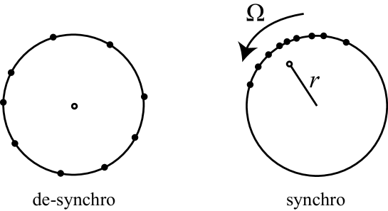
where . The order parameter gives the centroid of oscillators. If , then the synchronization occurs, while if is nearly equal to zero, the oscillators are uniformly distributed (de-synchronization), see Fig. 1.
Remark 2.1.
The coupling strength is the key bifurcation parameter that determines whether the dynamics becomes synchronous or de-synchronous, and it is important to obtain the bifurcation diagram of for the study of the edge of bifurcation. In this paper, we address the case where is large and consider the continuous limit of (2.1) as , namely, the infinite-dimensional Kuramoto model given by
| (2.4) |
where is the density of oscillators at a phase parameterized by natural frequency and time ,
is the drift velocity of the oscillators, and
is the order parameter of a solution .
For any ,
the trivial steady state solution of (2.4) exists
(i.e. a completely incoherent state given by for any ) and it corresponds to the de-synchronous state .
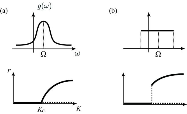
Kuramoto [7] conjectured that a bifurcation diagram of is given as Fig. 2 (a):
Kuramoto conjecture
Suppose that and natural frequencies ’s are distributed according to an even and unimodal function about its mean value with (this is true for Fig. 2 (a)). If , then is asymptotically stable, while if , the synchronous state emerges and is asymptotically stable for some given by
| (2.5) |
(see [12] for Kuramoto’s discussion).
The critical value is called the Kuramoto transition point. Then, Chiba [2] mathematically formulated this problem and proved the Kuramoto conjecture. See [2] for the precise statement.
It is known that the type of bifurcation strongly depends on the assumption for , especially for the sign of . For example, when is a uniform distribution (i.e. ), the bifurcation diagram is given as Fig. 2 (b). In this paper, as a reservoir, we consider both cases (a) is Gaussian (b) is a uniform distribution.
3 Reservoir computing with the Kuramoto model
We introduce the finite-dimensional Kuramoto model with an input term
| (3.1) |
where , denotes the phase of an -th oscillator on a circle, denotes its natural frequency, is a coupling strength, is the number of oscillators, is a constant and is an input. The case is the (usual) Kuramoto model (2.1). In reservoir computing, we take a sufficiently small and treat the input-aware model. The order parameter is similarly defined by (2.2). In addition, we define the -th order parameter of by
Similarly to Section 2, we consider the continuous limit of (3.1) as : with given natural frequency at time , satisfies the continuity equation
| (3.2) |
where is the density of oscillators at a phase parameterized by a natural frequency at time , is the drift velocity of the oscillators, and is the order parameter of . The -th order parameter is defined as
| (3.3) |
We propose reservoir computing with the infinite-dimensional Kuramoto model (3.2) as follows:
Reservoir computing and its purpose.
The reservoir computing with (3.2) consists of mappings , where is an output function. The map is defined by a solution of (3.2). Our purpose is to find the mapping (readout) so that
for a given target function , where is a certain norm or metric. For a finite dimensional problem, usually a readout is given by a matrix. However, since (3.2) is an infinite dimensional dynamical system, a readout may be a linear operator on an infinite dimensional space. Thus, we consider the following linear integral operator
| (3.4) |
where is a linear integral operator with an integral kernel .
Hence, the purpose of our reservoir computing is to find a suitable function such that
holds.
For mathematical analysis, we always assume that and it is real-valued in this paper. It is important to note that our reservoir computing (3.4) is convenient because it is expressed by the -th order parameters as follows. The integral kernel has a Fourier expansion
Then, by the definition (3.3) of , we rewrite as
Hence, the output of our reservoir computing can be represented as
| (3.5) |
This is an easily implementable setting and we can compute and numerically by using these formulae. Before giving its numerical algorithm, we consider mathematical results in the next section.
4 Approximation ability
As mentioned in the previous section, the approximation ability of reservoir computing (3.4) is essentially determined by the property of . In this section, we focus on the analysis of . Our main results are the following:
Theorem 4.1.
Let , and mean value of . Suppose that is bounded and continuous on .
Remark 4.2.
A few remarks are in order.
-
(a)
The system (3.2) for always has the steady state (de-synchronous state). In this case, for . Thus, we are interested in a non-trivial steady state. For example, when is even and unimodal or uniform distribution, it has a non-trivial steady state after the bifurcation to the synchronous state as in Fig. 2. In this case, in general (see Theorem 4.6 below).
- (b)
Corollary 4.3.
Our main results mean that the Kuramoto reservoir has almost the same approximation ability as the Fourier basis when for any , and is sufficiently small. See Theorem 4.6 for a sufficient condition for .
To prove Theorem 4.1, we use the following lemma, which is easily proved by integrating .
Lemma 4.4.
Let and . A steady state solution of (3.2) is given as
where is the Dirac delta function and is the -st order parameter of .
Proof of Theorem 4.1.
In order to prove the statement (ii), it is enough to show the statement (i). In fact, for the system (3.2), change the variables by
Then, it is easy to verify that the system is reduced to the case . More precisely, let be the order parameters for the case . Then we can calculate as
Therefore, once we prove when is a steady state, we conclude the statement (ii).
Suppose and , and let be a steady state. By Lemma 4.4, its -th order parameters are expressed as
Since is an even function about , we write
By Euler’s formula, this implies that is a real number for any as
| (4.2) |
As for , by making the change , we have
where
This implies if is odd (this fact will be used later). For any , we can also write as
and by making the change for the second integral, we have
| (4.3) |
Thus, and the proof of Theorem 4.1 is completed. ∎
To prove Corollary 4.3, we use the following lemma.
Lemma 4.5.
Let be a family of elements in a Hilbert space with inner product . Suppose that if and for any . Then is complete in .
Proof of Corollary 4.3.
Define by
For any , we suppose
for any . Put . If is bounded and continuous, , and is sufficiently small, then the map is one-to-one and of . Hence, the inverse function theorem gives
for any . Since is an orthogonal basis of , this implies that
Since if is sufficiently small, we have . Therefore, is a complete basis of by Lemma 4.5. Thus, we conclude Corollary 4.3. ∎
Now we give a sufficient condition for .
Theorem 4.6.
Assume that is either uniform distribution or even and unimodal function satisfying with the mean value . Then, there exists such that when , the constants given in Theorem 4.1 are nonzero for .
Corollary 4.7 (edge of bifurcation).
Corollary 4.7 immediately follows from Corollary 4.3 and Theorem 4.6.
Thus, we can express any function in as a linear combination of the order parameters of the system (3.2).
According to (3.5), we can find numbers (i.e. readout ) to obtain any function .
In the proof of Theorem 4.6, we use the second mean value theorem for definite integrals.
Lemma 4.8.
Let . Suppose is integrable and is monotone and bounded. Then there exists such that
Proof of Theorem 4.6.
It is trivial that by the definition. Hence, we assume . We prove the theorem only for the even and unimodal case, since the proof for the uniform distribution is similar. Since we assume , the constant is positive because of (2.5) (). Thus, we assume . By (4.2) and (4.3), is given by
(for the uniform distribution , we can calculate this integral and a proof is more easy).
First, is estimated as follows: By , we have
Due to Lemma 4.8, there exists such that
We estimate it around the bifurcation point (, and ) as
where we used because is an even function. The first integral is calculated as
(I) Suppose that is an odd number. Then, the above value is zero. Further, we have proved in the proof of Theorem 4.1 that . Thus, we have
To estimate it, define
where we put . Note that corresponds to . Then, we can verify that and
This proves that for small and there exists such that for . Note that is independent of because so is the factor .
(II) Suppose is an even number. In this case, and
| (4.4) |
Let us estimate the third term . We apply Lemma 4.8 with
Let us show that is monotonically increasing. It is easy to see that the integral exists and for and . This yields
for any . Hence, Lemma 4.8 is applicable to obtain
To calculate it, note that
when . This provides
where is a small positive number. The second term is of order as . For the first term, we can verify that it is nonzero and as . Putting
we obtain
| (4.5) |
Now we have estimations of all three terms of (4.4) for small . Case (II-1) If the third term is the leading term as , because . Case (II-2) If the first term is the leading term as (it may happen, for instance, accidentally ), then obviously . Case (II-3) If the second term is the leading term (it happens when the first and the third terms cancel each other). Then, the proof is the same as the case (I). For even , we can verify that and
Thus, we obtain .
This completes the proof of Theorem 4.6. ∎
In summary, we have obtained the following results to explain the edge of bifurcation:
-
•
We need (after bifurcation) because when , the trivial steady state is stable.
-
•
In particular, just after the bifurcation , we could prove .
-
•
We need because when , Corollary 4.3 does not hold. This means that we need a bifurcation from the steady state to periodic state (if , the bifurcation is from the steady state to the steady state).
-
•
Under the situation above, consists of the basis and we can approximate any function by using (3.5).
5 Experiments
Based on the above argument, we demonstrated the performance around the edge of bifurcation in the Kuramoto reservoir computing model using numerical simulation. Two tasks were used to evaluate the performance: a prediction task and a transformation task.
Since the -th order parameter can be numerically computed, we can obtain an approximate vector of in the following steps: it is an implementable model by the following procedure based on (3.5).
Algorithm. (Kuramoto reservoir computing)
Require: Data set (input/target) and hyperparameter .
-
1.
For training time , solve
(note that by the definition).
-
2.
Calculate (Moore-Penrose inverse).
-
3.
Return .
As above, we can indeed obtain the approximation of (i.e. the real Fourier series of an integral kernel in (3.4)) and use our reservoir computing for tasks such as time series prediction.
5.1 Prediction task
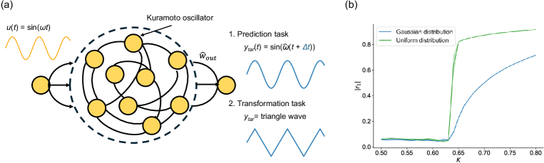
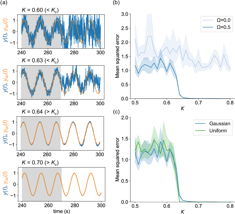
In this task, reservoir computing predicted the waveform one step after the input waveform. Fig. 3 (a) shows the composition of the Kuramoto reservoir computing system given in (3.4). oscillators receive the input (3.1), and is the output by the product of and (3.5). Note that was trained using during the training period. The training period to obtain was set to be 30 (s), and the testing period to the output was set to be 30 (s). These training and tests were performed after 240 (s) to stabilize the order parameters. In the prediction task, was , and was . The values of these parameters are summarized in Table 1 below.
The of each oscillator in the Kuramoto model was obtained from the distribution. We simulated two cases; the Gaussian distribution with mean and standard deviation 0.4, or uniform distribution on the interval (i.e. the mean value was also ). When the parameters were set in this way, the bifurcation points were (Gaussian distribution), (uniform distribution), respectively (Fig. 3 (b)). The reservoir computing performance was quantified by the mean squared error represented as
where is the number of the test step. As a result, the Kuramoto reservoir computing could predict the sine-wave one step after the input when (Fig. 4 (a)). The mean squared error was large when , and the sine-wave was not well predicted, however, it became smaller when exceeded (Fig. 4 (b)). On the other hand, if =0, the mean squared error remained large even when . In comparison with the case where was uniformly distributed, for the Gaussian case, the mean squared error still existed when was around (Fig. 4 (c)). This is because, for the Gaussian, the order parameter continuously changes at , while for the uniform distribution, it suddenly jumps to the value (see Fig. 2 and Fig. 3 (b)).
| Parameter | Description | Value |
|---|---|---|
| the number of oscillators | 500 | |
| time step | 0.01 (s) | |
| coefficient of the input | 0.01 | |
| angular velocity of the input signal | 0.5 (rad/s) | |
| input signal | ||
| target signal |
5.2 Transformation task
In this task, the reservoir computing was evaluated for performance through the conversion of the input waveform to another waveform. Here, the input was set to a sine-wave and to a triangle wave with the same period as the input signal (Fig. 5 (a)). Other parameters were the same as those set in the prediction task.
When , the Kuramoto reservoir computing could convert the sine-wave and generate the triangle wave when (Fig. 5 (a)). As with the prediction task, the mean squared error was large when , and the triangle wave was not well generated, but it became smaller when exceeded (Fig. 5 (b)). On the other hand, when =0, the mean squared error remained large even when . For the case where was uniformly distributed, as in the previous task, a difference in the mean squared error appeared when was around (Fig. 5 (c)). The common results obtained from these two tasks suggest that the Kuramoto reservoir can approximate various types of target function just after the bifurcation, which supports our mathematical results.

Acknowledgment
This work was supported by JST, CREST Grant Number JPMJCR2014, Japan (to HC and KT), JST Moonshot R&D Program Grant Number JPMJMS2023, Japan (to TS).
References
- [1] Thomas L Carroll. Do reservoir computers work best at the edge of chaos? Chaos: An Interdisciplinary Journal of Nonlinear Science, 30(12), 2020.
- [2] Hayato Chiba. A proof of the Kuramoto conjecture for a bifurcation structure of the infinite-dimensional Kuramoto model. Ergodic Theory and Dynamical Systems, 35(3):762–834, 2015.
- [3] James P Crutchfield and Karl Young. Computation at the onset of chaos. Entropy, complexity, and the physics of information, 8:223, 1990.
- [4] Ken Goto, Kohei Nakajima, and Hirofumi Notsu. Twin vortex computer in fluid flow. New Journal of Physics, 23(6):063051, 2021.
- [5] Herbert Jaeger. The “echo state” approach to analysing and training recurrent neural networks-with an erratum note. Bonn, Germany: German National Research Center for Information Technology GMD Technical Report, 148(34):13, 2001.
- [6] Y. Kuramoto. Self-entrainment of a population of coupled non-linear oscillators. In International Symposium on Mathematical Problems in Theoretical Physics, volume 39, pages 420–422. Springer, Berlin, 1975.
- [7] Y. Kuramoto. Chemical oscillations, waves, and turbulence. Springer Series in Synergetics, 19. Springer-Verlag, Berlin, 1984.
- [8] Chris G Langton. Computation at the edge of chaos: Phase transitions and emergent computation. Physica D: nonlinear phenomena, 42(1-3):12–37, 1990.
- [9] Mantas Lukoševičius and Herbert Jaeger. Reservoir computing approaches to recurrent neural network training. Computer science review, 3(3):127–149, 2009.
- [10] Thomas Natschläger, Wolfgang Maass, and Henry Markram. The “liquid computer”: A novel strategy for real-time computing on time series. Telematik, 8(ARTICLE):39–43, 2002.
- [11] Norman H Packard. Adaptation toward the edge of chaos. Dynamic patterns in complex systems, 212:293–301, 1988.
- [12] Steven H Strogatz. From Kuramoto to Crawford: exploring the onset of synchronization in populations of coupled oscillators. Physica D: Nonlinear Phenomena, 143(1-4):1–20, 2000.
- [13] Gouhei Tanaka, Toshiyuki Yamane, Jean Benoit Héroux, Ryosho Nakane, Naoki Kanazawa, Seiji Takeda, Hidetoshi Numata, Daiju Nakano, and Akira Hirose. Recent advances in physical reservoir computing: A review. Neural Networks, 115:100–123, 2019.
- [14] Liang Wang, Huawei Fan, Jinghua Xiao, Yueheng Lan, and Xingang Wang. Criticality in reservoir computer of coupled phase oscillators. Phys. Rev. E, 105:L052201, May 2022.
- [15] Toshiyuki Yamane, Seiji Takeda, Daiju Nakano, Gouhei Tanaka, Ryosho Nakane, Shigeru Nakagawa, and Akira Hirose. Dynamics of reservoir computing at the edge of stability. In Neural Information Processing, pages 205–212, Cham, 2016. Springer International Publishing.
- [16] Min Yan, Can Huang, Peter Bienstman, Peter Tino, Wei Lin, and Jie Sun. Emerging opportunities and challenges for the future of reservoir computing. Nature Communications, 15:2056, 03 2024.
- [17] Zhihao Zuo, Zhongxue Gan, Yuchuan Fan, Vjaceslavs Bobrovs, Xiaodan Pang, and Oskars Ozolins. Self-evolutionary reservoir computer based on Kuramoto model. arXiv preprint arXiv:2301.10654, 2023.