Optimal camera-robot pose estimation in linear time from points and lines

Abstract

Camera pose estimation is a fundamental problem in robotics. This paper focuses on two issues of interest: First, point and line features have complementary advantages, and it is of great value to design a uniform algorithm that can fuse them effectively; Second, with the development of modern front-end techniques, a large number of features can exist in a single image, which presents a potential for highly accurate robot pose estimation. With these observations, we propose AOPnP(L), an optimal linear-time camera-robot pose estimation algorithm from points and lines. Specifically, we represent a line with two distinct points on it and unify the noise model for point and line measurements where noises are added to 2D points in the image. By utilizing Plücker coordinates for line parameterization, we formulate a maximum likelihood (ML) problem for combined point and line measurements. To optimally solve the ML problem, AOPnP(L) adopts a two-step estimation scheme. In the first step, a consistent estimate that can converge to the true pose is devised by virtue of bias elimination. In the second step, a single Gauss-Newton iteration is executed to refine the initial estimate. AOPnP(L) features theoretical optimality in the sense that its mean squared error converges to the Cramér-Rao lower bound. Moreover, it owns a linear time complexity. These properties make it well-suited for precision-demanding and real-time robot pose estimation. Extensive experiments are conducted to validate our theoretical developments and demonstrate the superiority of AOPnP(L) in both static localization and dynamic odometry systems.

¹School of Data Science, Chinese University of Hong Kong, Shenzhen, Shenzhen, China
²Key Laboratory of Systems and Control, Institute of Systems Science, Academy of Mathematics and Systems Science, Chinese Academy of Sciences, Beijing, China
³System Hub, Hong Kong University of Science and Technology (Guangzhou), Guangzhou, China
⁴Australian Center for Field Robotics, School of Aerospace, Mechanical and Mechatronic Engineering, The University of Sydney, Sydney, Australia

1 Introduction

1.1 Background

Robot pose estimation refers to inferring the position and orientation of a robot in a specific coordinate system by using sensor measurements. As one of the most fundamental techniques in many robot applications, such as robot navigation, robotic grasping, and simultaneous localization and mapping (SLAM), pose estimation is an important topic in robotics and has been extensively investigated [1, 2, 3]. In virtue of low cost, high energy efficiency, and the ability to generate high-resolution images with detailed visual context, cameras have been a commonly used sensor for robot pose estimation.

One branch of visual-based methods utilizes the camera projection model and the correspondences between extracted features in the image plane and their 3D positions in the global frame to estimate the camera pose. The most commonly used feature is point features, which corresponds to the perspective-n-point (PnP) problem [4, 5, 6]. Another prevalent feature is line features, and the perspective-n-line (PnL) problem needs to be solved [7, 8, 9]. On the one hand, line features are more robust in texture-less or repetitive scenes without enough distinctive points. This is likely to occur in man-made structures. While on the other hand, given a line correspondence, there still exists a shift of the line along its direction. In addition, line features may be partially observed due to occlusions. Existing PnL methods are not yet as accurate as PnP ones with enough distinctive point features [10]. Therefore, some works utilize both point and line features for camera pose estimation, which yields the so-called PnPL problem [10, 11].

Accurate pose acquisition is crucial for many modern robot applications, such as surgical robots [12], implicit mapping based on neural radiance fields [13], and large-scale SLAM [14]. It is noteworthy that with the development of feature detectors and descriptors, a large number of features can exist in a single image, which brings great potential for highly precise pose estimation. One idea to fully exploit the large sample feature measurements is to devise a consistent and asymptotically efficient estimate, which converges to the true pose with a minimum covariance as the feature number increases. We note that the existing methods generally ignore the modeling of measurement noises and lack elaborate design from the perspective of statistical estimation theory. As a result, they are usually inconsistent due to the nonlinear property of the pinhole camera projection model. In what follows, we will give a literature review.

1.2 Related work

PnP problem: As points are easier to handle mathematically than lines in camera pose estimation, the PnP problem was first studied. Some works consider a fixed number of points. Since the degree of the pose is six and each point correspondence produces two independent equations, the minimal case is $n=3$, which corresponds to the P3P problem [15, 16]. There are also P4P [17] and P5P [18] solvers for $n=4$ and $n=5$, respectively. These fix-point solutions are sensitive to noises and generally embedded in a random sample consensus (RANSAC) framework for robust estimation. Most PnP solvers, however, can cope with a flexible number of points by formulating a least-squares problem. The optimization methods can be categorized into iterative and noniterative algorithms. Iterative methods start with an initial value and solve the problem using an iterative algorithm, e.g., the GN and Levenberg-Marquardt (LM) methods [19, 20, 6]. Due to the nonconvexity of the problem, without a good initialization, iterative methods can only result in a local minimum. Early noniterative methods usually have a high computational complexity. The first well-known $O(n)$ solver is EPnP [4], which utilizes linearization techniques. Direct linear transformation (DLT) is another linear formulation [21]. Apart from linearization techniques, polynomial solvers that do not ignore the constraints on rotation have become mainstream [22, 23, 24]. They estimate the pose by solving a system of polynomial equations and can generally achieve a better performance than linear methods which ignore constraints. Noniterative solutions are sometimes used as the initial value for iterative algorithms.

PnL problem: The early PnL research emerged in the 1990s for the reason that line features are generally more robust than point features, especially in texture-less or repetitive scenes. Note that each line correspondence provides two independent equations. Thus, the minimal case is also $n=3$, which results in the P3L problem [25]. For nonminimal flexible cases, early works mainly focused on error function formulation and iterative solutions [26]. Because of nonconvexity, iterative methods also face the possibility of converging to local minima [27, 28]. In terms of noniterative methods, the DLT formulations can vary for different line parameterizations. The classical DLT method parameterizes a 3D line by its two endpoints and constructs homogeneous equations based on the constraint that the projection of the endpoints should be on the 2D line [21]. Přibyl et al. [29] used the Plücker coordinates to represent a 3D line and proposed a novel DLT method. Compared with linear methods, polynomial solvers that consider the rotation constraints need fewer lines and can usually obtain a more accurate solution for a small $n$ [30, 31, 7, 32]. However, they are more computationally demanding and may encounter numerical problems [26].

PnPL problem: There is a limited number of approaches that estimate the camera pose utilizing both points and lines. The minimal case was addressed in [33, 34]. For nonminimal cases, DLT methods are straightforward since the homogeneous equations for both points and lines have already been established in previous works [21]. Extending the existing PnP methods to the PnPL counterparts by elaborately formulating the line projection error is another practical approach, for instance, Vakhitov et al. [10] developed EPnP and OPnP to EPnPL and OPnPL, respectively, and EPnP and DLS are extended to EPnPLU and DLSLU, respectively in [11]. Li et al. adopted the Cayley parametrization for the rotation matrix and constructed a polynomial system by the first-order optimality condition [35]. Recently, certifiably optimal solvers were proposed with sum-of-squares relaxation [36] and semidefinite relaxation [37].

Uncertainty-aware PnP(L) problem: Most existing works do not consider measurement noises contained in features. Since the extracted features are inevitably corrupted by noises, the uncertainty-aware methods that explicitly model noises are likely to achieve higher accuracy. Among them, the uncertainty in 2D features was considered and a weighted least-squares problem by using the squared Mahalanobis distance was formulated in [30, 38, 5, 35, 11]. Recently, Vakhitov et al. [11] estimated both 2D and 3D uncertainty to enhance estimation performance. However, it needs prior information of an initial pose or the average scene depth. We remark that although the above methods have considered the noise model, they do not analyze noise propagation and the effect on the final estimate. The lack of statistical analysis and optimization from the perspective of estimation theory makes them not asymptotically unbiased and consistent. CPnP [39] can obtain a consistent estimate, however, it cannot theoretically guarantee asymptotic efficiency, and it is only applicable to point features.

1.3 Main results

This paper investigates the camera-robot pose estimation problem with large sample features. We propose a uniform estimator that can take point features, line features, or both as measurements. In terms of estimation accuracy, the proposed estimator is optimal in the large sample case—it optimally solves the maximum likelihood (ML) problem and its covariance reaches a theoretical lower bound as the number of features increases. In terms of computation speed, it has a linear time complexity—the consuming time linearly grows with respect to the feature number. With a large number of features, our estimator provides an appropriate solution for highly precise and real-time robot pose estimation.

The main contributions of this paper are summarized as follows:

1. By representing a line with two distinct points on it, we unify the camera noise model in which measurement noises are added to 2D point projections in the image. In addition, by utilizing the Plücker coordinates for line parameterization, we construct the residuals for line features and formulate a uniform ML problem for combined point and line measurements.

2. We propose a uniform pose estimation framework for combined point and line measurements. The framework has linear time complexity and is asymptotically optimal. The core of the framework is a two-step estimation scheme, which asymptotically solves the ML problem. In the first step, we devise a consistent pose estimate that converges to the true pose as features increase. In the second step, we execute a single Gauss-Newton (GN) iteration and prove that the refined estimate asymptotically reaches the theoretical lower bound—Cramér-Rao bound (CRB).

3. The framework also incorporates two modules to facilitate the stability and applicability of the estimator in real scenarios. The first is data preprocessing, which normalizes the scale of data to promote numerical stability. The second is consistent noise variance estimation by solving a generalized eigenvalue problem, which is a prerequisite for the proposed two-step pose estimator in case of unknown noise statistical characteristics.

4. We perform extensive experiments with both synthetic and real-world data to verify the theoretical developments and compare the proposed estimator with state-of-the-art ones. The experiment results demonstrate the superiority of our algorithm in terms of estimation accuracy and computation speed, not only for robot relocalization in a known map but also for SLAM in an unknown environment.

2 Preliminaries

To facilitate the readability of the subsequent technical part, in this section, we give some preliminaries on notations, probability and statistics, rigid transformation, and GN iterations on the manifold of ${\rm SO}(3)$.

2.1 Notations

For a vector $\bf v$, $[{\bf v}]_{i}$ denotes its $i$-th element, $\|{\bf v}\|_{\bm{\Sigma}}^{2}={\bf v}^{\top}{\bm{\Sigma}}^{-1}{\bf v}$, and ${\rm diag}(\bf v)$ returns a diagonal matrix with $\bf v$ being its diagonal elements. Given a matrix ${\bf M}$, $\|{\bf M}\|_{\rm F}$ returns its Frobenius norm, and ${\rm vec}({\bf M})$ yields a vector by concatenating the columns of ${\bf M}$. If ${\bf M}$ is a square matrix, then ${\rm tr}({\bf M})$ represents its trace, and ${\rm det}({\bf M})$ denotes its determinant. If ${\bf M}$ has real eigenvalues, then $\lambda_{\rm min}({\bf M})$ and $\lambda_{\rm max}({\bf M})$ denote the minimum and maximum eigenvalues of ${\bf M}$, respectively. We use $\times$ to denote the cross product and $\otimes$ to denote the Kronecker product. We denote the identity matrix of size $n$ as ${\bf I}_{n}$ and the zero matrix of size $n\times m$ as ${\bf 0}_{n\times m}$. For a quantity ${\bf x}$ corrupted by noise, we use ${\bf x}^{o}$ to denote its noise-free counterpart.

2.2 Some notions in probability and statistics

Convergence in probability. The small $o_{p}$ notation $X_{n}=o_{p}(a_{n})$ means that the sequence $(X_{n}/a_{n})$ converges to zero in probability. That is, for any $\varepsilon>0$,

$$\lim_{n\rightarrow\infty}\mathbb{P}(|X_{n}/a_{n}|>\varepsilon)=0.$$

Stochastic boundedness. The big $O_{p}$ notation $X_{n}=O_{p}(a_{n})$ means that the sequence $(X_{n}/a_{n})$ is stochastically bounded. That is, for any $\varepsilon>0$, there exists a finite $M$ and a finite $N$ such that for any $n>N$,

$$\mathbb{P}(|X_{n}/a_{n}|>M)<\varepsilon.$$

The following notions are established on the premise that given $n$ measurements $\mathcal{Y}_{n}\triangleq\{{\bf y}_{1},\ldots,{\bf y}_{n}\}$, $\hat{\bm{\theta}}_{n}$ is an estimate of some unknown parameter ${\bm{\theta}}^{o}$.

Consistent and $\sqrt{n}$-consistent estimate. The estimate $\hat{\bm{\theta}}_{n}$ is called a (weakly) consistent estimate of ${\bm{\theta}}^{o}$ if

$$\hat{\bm{\theta}}_{n}-{\bm{\theta}}^{o}=o_{p}(1).$$

Furthermore, $\hat{\bm{\theta}}_{n}$ is called a $\sqrt{n}$-consistent estimate of ${\bm{\theta}}^{o}$ if

$$\hat{\bm{\theta}}_{n}-{\bm{\theta}}^{o}=O_{p}(1/\sqrt{n}).$$

It is noteworthy that $\sqrt{n}$-consistent includes two implications: The estimate $\hat{\bm{\theta}}_{n}$ is consistent, i.e., $\hat{\bm{\theta}}_{n}$ converges to ${\bm{\theta}}^{o}$ in probability; The convergence rate is $1/\sqrt{n}$.

(Asymptotically) unbiased estimate. The bias of an estimate $\hat{\bm{\theta}}_{n}$ is equal to its expectation minus the true value, i.e., ${\rm Bias}(\hat{\bm{\theta}}_{n})=\mathbb{E}[\hat{\bm{\theta}}_{n}]-{\bm{\theta}}^{o}$. If ${\rm Bias}(\hat{\bm{\theta}}_{n})=0$, we call $\hat{\bm{\theta}}_{n}$ an unbiased estimate of ${\bm{\theta}}^{o}$. In particular, if $\lim_{n\rightarrow\infty}{\rm Bias}(\hat{\bm{\theta}}_{n})=0$, we call $\hat{\bm{\theta}}_{n}$ an asymptotically unbiased estimate. It is noteworthy that an asymptotically unbiased estimate $\hat{\bm{\theta}}_{n}$ may not necessarily be unbiased given a finite $n$.

(Asymptotically) efficient estimate. An unbiased estimate $\hat{\bm{\theta}}_{n}$ is said to be efficient if its covariance ${\rm cov}(\hat{\bm{\theta}}_{n})$ equals the theoretical lower bound — Cramér-Rao bound (CRB). In particular, $\hat{\bm{\theta}}_{n}$ is called asymptotically efficient if it is asymptotically unbiased, and $\lim_{n\rightarrow\infty}{\rm cov}(\sqrt{n}\hat{\bm{\theta}}_{n})=n{\rm CRB}$. CRB can be obtained from the Fisher information matrix $\bf F$ as ${\rm CRB}={\bf F}^{-1}$, and $\bf F$ is the covariance of the derivative of the log-likelihood function $\ell({\bm{\theta}};\mathcal{Y}_{n})$ evaluated at the true parameter ${\bm{\theta}}^{o}$:

$${\bf F}=\mathbb{E}\left[\frac{\partial\ell({\bm{\theta}};\mathcal{Y}_{n})}{\partial{\bm{\theta}}}\frac{\partial\ell({\bm{\theta}};\mathcal{Y}_{n})}{\partial{\bm{\theta}}^{\top}}\bigg{|}{\bm{\theta}}^{o}\right].$$

2.3 Rigid transformation

The (proper) rigid transformations, or said relative poses, include rotations and translations. In the 3D Euclidean space, the translation is depicted by a vector ${\bf t}\in\mathbb{R}^{3}$. The rotation can be characterized by a rotation matrix $\bf R$. Specifically, rotation matrices belong to the special orthogonal group

$${\rm SO}(3)=\{{\bf R}\in\mathbb{R}^{3\times 3}\mid{\bf R}^{\top}{\bf R}={\bf I}_{3},{\rm det}({\bf R})=1\}.$$

The group operation is the usual matrix multiplication, and the inverse is the matrix transpose. The group ${\rm SO}(3)$ forms a smooth manifold, and the tangent space to the manifold (at the identity) is denoted as the Lie algebra $\mathfrak{so}(3)$ which is comprised of all $3\times 3$ skew-symmetric matrices. Every $3\times 3$ skew-symmetric matrix can be generated from a vector ${\bf s}\in\mathbb{R}^{3}$ via the hat operator:

$${\bf s}^{\wedge}=\begin{bmatrix}s_{1}\\ s_{2}\\ s_{3}\end{bmatrix}^{\wedge}=\begin{bmatrix}0&-s_{3}&s_{2}\\ s_{3}&0&-s_{1}\\ -s_{2}&s_{1}&0\end{bmatrix}\in\mathfrak{so}(3).$$ (1)

Conversely, the vee operator retrieves the vector from a skew-symmetric matrix:

$$\left({\bf s}^{\wedge}\right)^{\vee}={\bf s}\in\mathbb{R}^{3}.$$

The exponential map ${\rm exp}:\mathfrak{so}(3)\rightarrow{\rm SO}(3)$, which coincides with standard matrix exponential, associates an element in the Lie algebra to a rotation matrix. Specifically, Rodrigues’ rotation formula reads that

$${\rm exp}\left({\bf s}^{\wedge}\right)={\bf I}_{3}+\frac{\sin(\|{\bf s}\|)}{\|{\bf s}\|}{\bf s}^{\wedge}+\frac{1-\cos(\|{\bf s}\|)}{\|{\bf s}\|^{2}}\left({\bf s}^{\wedge}\right)^{2}.$$

Conversely, the logarithm map ${\rm log}:{\rm SO}(3)\rightarrow\mathfrak{so}(3)$ associates a rotation matrix ${\bf R}\neq{\bf I}_{3}$ to a skew-symmetric matrix:

$${\rm log}({\bf R})=\frac{\phi({\bf R}-{\bf R}^{\top})}{2\sin(\phi)}\leavevmode\nobreak\ \leavevmode\nobreak\ \text{with}\leavevmode\nobreak\ \leavevmode\nobreak\ \phi=\cos^{-1}\left(\frac{{\rm tr}(\bf R)-1}{2}\right).$$

One can further write ${\rm log}({\bf R})^{\vee}=\phi{\bf n}$, where the unit vector $\bf n$ denotes the rotation axis, and $\phi$ is the rotation angle. It is noteworthy that the exponential map is bijective if we confine its domain to the open ball $\{{\bf s}\mid\|{\bf s}\|<\pi\}$, and its inverse is the logarithm map.

Suppose the relative pose of the second frame with respect to (w.r.t.) the first frame is $({\bf R},{\bf t})$, and the coordinates of a 3D point in the second frame is ${\bf X}$. Then the coordinates of the point in the first frame is ${\bf R}{\bf X}+{\bf t}$.

2.4 Gauss-Newton method on ${\rm SO}(3)$

The GN method is usually applied to iteratively solve a nonlinear least-squares optimization problem. It is an approximation of Newton’s method and has the advantage that second derivatives are not required. Specifically, it linearly approximates residuals through the first-order Taylor polynomial, and then optimally solves the resulting quadratic problem with a closed-form solution. When it comes to an optimization problem over the manifold of ${\rm SO}(3)$, the standard GN method needs to be modified with some techniques to ensure that the updated value after each iteration also belongs to ${\rm SO}(3)$.

Consider the following optimization problem:

$$\mathop{\rm minimize}\limits_{{\bf R}\in{\rm SO}(3),{\bf t}\in\mathbb{R}^{3}}\leavevmode\nobreak\ \|{\bf r}({\bf R},{\bf t})\|^{2}.$$ (2)

Note that the rotation in the 3D space has three degrees, while the rotation matrix $\bf R$ has nine elements, which is overparameterized. If we directly optimize over $\bf R$, the Jacobian matrix may not have full column rank, and the updated value of $\bf R$ is generally not an element of ${\rm SO}(3)$. To overcome this issue, we can introduce a retraction $\mathcal{R}_{\bf R}$, which is a bijective map between an element ${\bf s}$ of the tangent space at $\bf R$ and a neighborhood of ${\bf R}\in{\rm SO}(3)$. The retraction used in this paper is

$$\mathcal{R}_{\bf R}({\bf s})={\bf R}\leavevmode\nobreak\ {\rm exp}({\bf s}^{\wedge}),\leavevmode\nobreak\ \leavevmode\nobreak\ {\bf s}\in\mathbb{R}^{3}.$$ (3)

Given an initial estimate $\hat{\bf R}\in{\rm SO}(3)$, using this retraction, the original problem (2) is converted into

$$\mathop{\rm minimize}\limits_{{\bf s,t}\in\mathbb{R}^{3}}\leavevmode\nobreak\ \|{\bf r}\left(\mathcal{R}_{\hat{\bf R}}({\bf s}),{\bf t}\right)\|^{2}.$$ (4)

The above reparameterization is usually called lifting. The main idea is to work in the tangent space defined at the current estimate $\hat{\bf R}$, which locally behaves as an Euclidean space. The Euclidean space has three dimensions, coinciding with the degree of a 3D rotation. Note that problem (4) is an optimization problem over an Euclidean space and thus can be solved utilizing the standard GN method. Once an updated $\hat{\bf s}$ is produced, we can obtain a refined rotation matrix $\mathcal{R}_{\hat{\bf R}}(\hat{\bf s})$ which naturally belongs to ${\rm SO}(3)$ via the retraction (3).

3 Problem formulation

3.1 Point and line models

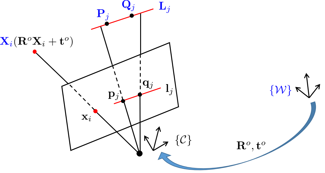
Figure 1: Illustration of point and line correspondences.

We consider a pinhole camera model and assume the intrinsic matrix of the camera is known by some means, such as a prior calibration. As such, without loss of generality, we assume the focal length $f=1$ and utilize normalized image coordinates to represent points in the image plane. Let $\{\mathcal{W}\}$ and $\{\mathcal{C}\}$ denote the world coordinate frame and camera coordinate frame, respectively. To estimate the relative pose of $\{\mathcal{W}\}$ w.r.t. $\{\mathcal{C}\}$, which is denoted by a rotation matrix ${\bf R}^{o}$ and a translation vector ${\bf t}^{o}$, suppose that there exist $n$ point correspondences $\{({\bf X}_{i},{\bf x}_{i})\}_{i=1}^{n}$ and $m$ line correspondences $\{({\bf L}_{j},{\bf l}_{j})\}_{j=1}^{m}$. Here, ${\bf X}_{i}\in\mathbb{R}^{3}$ denotes the $i$-th 3D point in the world frame, and ${\bf x}_{i}\in\mathbb{R}^{2}$ represents its 2D projection (in the form of normalized image coordinates) in the image plane. Let ${\bf X}_{i}^{h}\triangleq[{\bf X}_{i}^{\top}\leavevmode\nobreak\ 1]^{\top}$ and ${\bf x}_{i}^{h}\triangleq[{\bf x}_{i}^{\top}\leavevmode\nobreak\ 1]^{\top}$ be the corresponding homogeneous coordinates. As illustrated in Figure 1, we have the following relationship:

$${\bf x}_{i}^{h}\approx{\bf R}^{o}{\bf X}_{i}+{\bf t}^{o}=[{\bf R}^{o}\leavevmode\nobreak\ \leavevmode\nobreak\ {\bf t}^{o}]{\bf X}_{i}^{h},$$ (5)

where $\approx$ denotes the equivalence relation that equates two values only with a nonzero scale difference. More specifically, the exact point projection function is given by [39]

$${\bf x}_{i}=h_{{\bf R}^{o},{\bf t}^{o}}({\bf X}_{i})\triangleq\frac{{\bf E}({\bf R}^{o}{\bf X}_{i}+{\bf t}^{o})}{{\bf e}_{3}^{\top}({\bf R}^{o}{\bf X}_{i}+{\bf t}^{o})},$$ (6)

where ${\bf E}=[{\bf e}_{1}\leavevmode\nobreak\ {\bf e}_{2}]^{\top}$, and ${\bf e}_{i}$ denotes the unit vector whose $i$-th element is $1$.

For the $j$-th line ${\bf L}_{j}$ in the world frame, we denote it by two distinct points ${\bf P}_{j}$ and ${\bf Q}_{j}$ on it and parameterize it with Plücker coordinates [21] as follows:

$${\bf L}_{j}\triangleq\left[({\bf P}_{j}\times{\bf Q}_{j})^{\top}\leavevmode\nobreak\ \leavevmode\nobreak\ ({\bf Q}_{j}-{\bf P}_{j})^{\top}\right]^{\top}\in\mathbb{R}^{6}.$$

Note that a line in the 3D space has a degree of four. Hence, the Plücker coordinates representation is overparameterized. Nevertheless, it is widely used in geometric computer vision since the projection of a line under this parameterization exhibits a linear form [21, 29, 40]. Similarly, we denote ${\bf l}_{j}$ (the projection of ${\bf L}_{j}$) by two distinct points ${\bf p}_{j}$ and ${\bf q}_{j}$ on it and parameterize it as ${\bf l}_{j}\triangleq{\bf p}_{j}^{h}\times{\bf q}_{j}^{h}\in\mathbb{R}^{3}$, where ${\bf p}_{j}^{h}\triangleq[{\bf p}_{j}^{\top}\leavevmode\nobreak\ 1]^{\top}$ and ${\bf q}_{j}^{h}\triangleq[{\bf q}_{j}^{\top}\leavevmode\nobreak\ 1]^{\top}$. Then, the linear line projection is expressed as [21]

$${\bf l}_{j}\approx\left[{\bf R}^{o}\leavevmode\nobreak\ \leavevmode\nobreak\ {\bf t}^{o\wedge}{\bf R}^{o}\right]{\bf L}_{j},$$ (7)

where the hat operator $\wedge$ has been defined in (1). It is worth mentioning that for the $j$-th line correspondence $({\bf L}_{j},{\bf l}_{j})$, their endpoints generally do not form point correspondences, i.e., ${\bf p}_{j}$ and ${\bf q}_{j}$ are generally not the projections of ${\bf P}_{j}$ and ${\bf Q}_{j}$, as shown in Figure 1.

3.2 ML problem

In the previous subsection, we have introduced the models of points and lines and the ideal projection geometry. In this part, we explicitly take measurement noises (or projection noises) into account and construct an ML problem from both point and line features. Specifically, we suppose noises are added to the projections of points. That is,

$${\bf x}_{i} =h_{{\bf R}^{o},{\bf t}^{o}}({\bf X}_{i})+\bm{\epsilon}_{{\bf x}_{i}}={\bf x}_{i}^{o}+\bm{\epsilon}_{{\bf x}_{i}},$$ (8)

$${\bf p}_{j} ={\bf p}_{j}^{o}+\bm{\epsilon}_{{\bf p}_{j}},\leavevmode\nobreak\ \leavevmode\nobreak\ \leavevmode\nobreak\ \leavevmode\nobreak\ \leavevmode\nobreak\ \leavevmode\nobreak\ {\bf q}_{j}={\bf q}_{j}^{o}+\bm{\epsilon}_{{\bf q}_{j}},$$ (9)

where the quantity $(\cdot)^{o}$ denotes the corresponding noise-free counterpart of $(\cdot)$, and $\bm{\epsilon}_{{\bf x}_{i}}$, $\bm{\epsilon}_{{\bf p}_{j}}$, and $\bm{\epsilon}_{{\bf q}_{j}}$ are measurement noises, which are assumed to be mutually independent and follow a Gaussian distribution $\mathcal{N}\left(0,\sigma^{2}{\bf I}_{2}\right)$.

Remark 1.

Note that for the line ${\bf l}_{j}$, we do not directly add a 3D noise vector to ${\bf l}_{j}^{o}$. Instead, we add a 2D noise to each of its endpoints. Although this modeling is more complicated and harder to handle, it is more in line with the fact that the original measurements of a camera are a series of points. This modeling also satisfies the intuition that longer line segments are less affected by the noises on their endpoints, i.e., the longer a line segment is, the more confident we are with the observation. Actually, adding noises to the endpoints of a line is widely used in the simulation of previous works [29, 26, 30, 7].

Based on the point measurement model (8), the residual for the $i$-th point is

$${\bf r}_{pi}({\bf R},{\bf t})={\bf x}_{i}-h_{{\bf R},{\bf t}}({\bf X}_{i}),$$ (10)

and the weight matrix is $\bm{\Sigma}^{-1}=\frac{1}{\sigma^{2}}{\bf I}_{2}$. However, the residual for the $j$-th line is not so straightforward since the 3D points associated with ${\bf p}_{j}$ and ${\bf q}_{j}$ are unknown. Let $\bar{\bf l}_{j}\triangleq\left[{\bf R}\leavevmode\nobreak\ \leavevmode\nobreak\ {\bf t}^{\wedge}{\bf R}\right]{\bf L}_{j}$. Note that ${\bf p}_{j}^{o}$ and ${\bf q}_{j}^{o}$ lie on $\bar{\bf l}_{j}^{o}\triangleq\left[{\bf R}^{o}\leavevmode\nobreak\ \leavevmode\nobreak\ {\bf t}^{o\wedge}{\bf R}^{o}\right]{\bf L}_{j}$. We have $\bar{\bf l}_{j}^{o\top}{\bf p}_{j}^{oh}=0$ and $\bar{\bf l}_{j}^{o\top}{\bf q}_{j}^{oh}=0$, which give

$$0=\bar{\bf l}_{j}^{o\top}{\bf p}_{j}^{h}-\bar{\bf l}_{j}^{o\top}\bm{\epsilon}_{{\bf p}_{j}}^{h},\leavevmode\nobreak\ \leavevmode\nobreak\ 0=\bar{\bf l}_{j}^{o\top}{\bf q}_{j}^{h}-\bar{\bf l}_{j}^{o\top}\bm{\epsilon}_{{\bf q}_{j}}^{h},$$ (11)

where $\bm{\epsilon}_{{\bf p}_{j}}^{h}$ and $\bm{\epsilon}_{{\bf q}_{j}}^{h}$ are the homogeneous coordinates of $\bm{\epsilon}_{{\bf p}_{j}}$ and $\bm{\epsilon}_{{\bf q}_{j}}$, respectively. The noise terms $\bar{\bf l}_{j}^{o\top}\bm{\epsilon}_{{\bf p}_{j}}^{h}$ and $\bar{\bf l}_{j}^{o\top}\bm{\epsilon}_{{\bf q}_{j}}^{h}$ in (11) follow the Gaussian distribution $\mathcal{N}\left(0,\sigma_{j}^{2}({\bf R}^{o},{\bf t}^{o})\right)$, where we use $\sigma_{j}^{2}({\bf R}^{o},{\bf t}^{o})$ to indicate that $\sigma_{j}^{2}$ is a function of ${\bf R}^{o}$ and ${\bf t}^{o}$. The explicit expression of $\sigma_{j}^{2}({\bf R}^{o},{\bf t}^{o})$ is $\sigma_{j}^{2}({\bf R}^{o},{\bf t}^{o})=[\bar{\bf l}_{j}^{o}]_{1:2}^{\top}{\bm{\Sigma}}[\bar{\bf l}_{j}^{o}]_{1:2}$, where $[\bar{\bf l}_{j}^{o}]_{1:2}$ denotes the first two elements of $\bar{\bf l}_{j}^{o}$. As a result, the residual for the $j$-th line is formulated as

$${\bf r}_{lj}({\bf R},{\bf t})=\begin{bmatrix}{\bf p}_{j}^{h\top}\\ {\bf q}_{j}^{h\top}\end{bmatrix}\left[{\bf R}\leavevmode\nobreak\ \leavevmode\nobreak\ {\bf t}^{\wedge}{\bf R}\right]{\bf L}_{j},$$ (12)

and the weight matrix is $\bm{\Sigma}_{j}^{-1}=\frac{1}{\sigma_{j}^{2}({\bf R}^{o},{\bf t}^{o})}{\bf I}_{2}$.

Finally, by combining the point residual (10) and line residual (12), the ML problem is formulated as

$$\begin{split}\mathop{\rm minimize}\limits_{{\bf R},{\bf t}}\leavevmode\nobreak\ &\frac{1}{n+m}\left(\sum_{i=1}^{n}\left\|{\bf r}_{pi}\right\|_{\bm{\Sigma}}^{2}+\sum_{j=1}^{m}\left\|{\bf r}_{lj}\right\|_{\bm{\Sigma}_{j}}^{2}\right)\\ \mathop{\rm subject\leavevmode\nobreak\ to}\leavevmode\nobreak\ &{\bf R}\in{\rm SO}(3),{\bf t}\in\mathbb{R}^{3},\end{split}$$ (13)

where we have abbreviated ${\bf r}_{pi}({\bf R},{\bf t})$ and ${\bf r}_{lj}({\bf R},{\bf t})$ to ${\bf r}_{pi}$ and ${\bf r}_{lj}$, respectively. A global solution to (13) is called an ML estimate, denoted as $\hat{\bf R}^{\rm ML}$ and $\hat{\bf t}^{\rm ML}$, and an algorithm that optimally solves (13) is termed an ML estimator. Note that the degrees of $\bf R$ and $\bf t$ are both $3$, and each point or line correspondence can provide $2$ independent equations. Hence, at least $n+m=3$ point/line correspondences are required to estimate the camera pose.

From the statistical theory, we know that under some regularity conditions, an ML estimate is consistent and asymptotically efficient. Thanks to the development of modern feature extraction techniques, a large number of features can exist in a single image. For example, Figure 2 shows two images from the ETH3D [41] and VGG [42] datasets, respectively. One image contains thousands of point features, and the other has hundreds of line features. The main problem of interest in this paper is to fully exploit the value of large sample features, which can be achieved by optimally solving the ML problem (13).

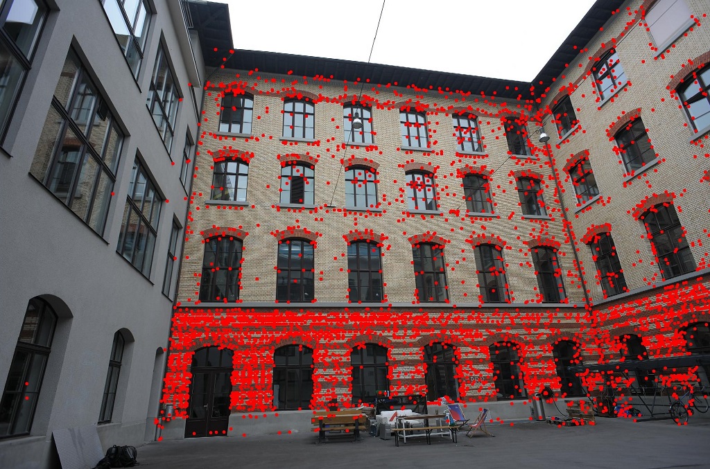
(a) Point features in the ETH3D dataset

(b) Line features in the VGG dataset

Figure 2: Large sample features extracted from a single image.

4 Algorithm framework

The ML problem (13) is nonconvex since the objective is nonconvex, and the ${\rm SO}(3)$ group is not a convex set. In addition, the covariance matrices $\bm{\Sigma}$ and $\bm{\Sigma}_{j},j=1,\ldots,m$ are unknown. As a result, a global solution to the ML problem is hard to obtain. When using a locally iterative method to solve the ML problem, e.g., the GN algorithm, it is required that the initial value falls into the attraction neighborhood of a global minimum, otherwise, we can only obtain a locally optimal solution.

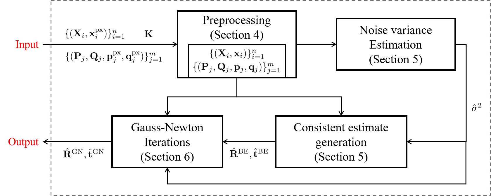
Figure 3: Overview of algorithm framework.

In this paper, our focus is to devise an algorithm that can yield an estimate, which owns the same asymptotic properties as the ML estimate. In other words, we are going to propose a consistent and asymptotically efficient estimator. The algorithm framework is shown in Figure 3. The input of our algorithm includes the camera intrinsic matrix $\bf K$, $n$ point correspondences, and $m$ line correspondences, where all 2D points are expressed as pixel coordinates $(\cdot)^{\rm px}$. The output is the estimate of the camera pose. Our algorithm consists of four components. In what follows, we will outline their functions respectively.

(1) Preprocessing. By drawing lessons from the existing literature [21, 29], points and lines need to be normalized to make an algorithm numerically stable. In practice, the main principle is that points and lines with large absolute values need to be normalized. For the detected 2D points, we convert their pixel coordinates into normalized image coordinates based on the camera’s intrinsic parameters. Take ${\bf x}_{i}^{\rm px}$ as example, and we have

$${\bf x}_{i}=[{\bf K}^{-1}]_{1:2}\begin{bmatrix}{\bf x}_{i}^{\rm px}\\ 1\end{bmatrix},$$

where $[{\bf K}^{-1}]_{1:2}$ denotes the first two rows of ${\bf K}^{-1}$. The line endpoints ${\bf p}_{j}$ and ${\bf q}_{j}$ can be obtained in the same way. For each 3D line ${\bf L}_{j}$, we move ${\bf P}_{j}$ and ${\bf Q}_{j}$ along the line direction such that $\|{\bf P}_{j}-{\bf Q}_{j}\|=\sqrt{3}$.

(2) Noise variance estimation. For a nonlinear and nonconvex optimization problem, solutions obtained by some relaxation-based methods are usually biased, and the bias is generally associated with the variance of measurement noises. Therefore, it is important to estimate noise variance in order to eliminate the bias, obtaining an asymptotically unbiased and consistent solution. The technical details of noise variance estimation will be presented in Section 5. The resulting consistent noise variance estimate will be utilized in the components of consistent estimate generation and GN iterations.

(3) Consistent estimate generation. We relax the original ML problem (13) to a generalized trust region subproblem (GTRS) whose global solution can be obtained. In addition, based on the noise variance estimate, we conduct bias elimination, which yields a consistent pose estimate. The consistent estimate serves as a good initial value for the following GN iterations to find the ML estimate. In addition, the consistent estimator has a closed-form expression and thus is computationally efficient. The technical details of consistent estimate generation will be presented in Section 5.

(4) Gauss-Newton iterations. Taking the consistent estimate as the initial value, the GN algorithm is executed to find the ML estimate. With the increase of the measurement number, the consistent estimate can converge into the attraction neighborhood of the global minimum of the ML problem (13), hence the ML estimate is achievable in the large sample case. It is worth noting that due to the SO(3) constraint on the rotation matrix and ${\bm{\Sigma}}_{j}$ in (13) being a function of the true pose, a modified GN algorithm instead of the standard one needs to be designed. The proposed GN iterations and the resulting asymptotic efficiency will be presented in Section 6 in detail.

5 Consistent estimator design

In this section, we will detail the initial consistent estimator in the first step. Subsection 5.1 is for the case of point features, Subsection 5.2 is for the case of line features, and the case of combined point and line features is described in Subsection 5.3.

5.1 Consistent estimation from point correspondences

Since ${\bf x}_{i}^{oh}$ is parallel to ${\bf R}^{o}{\bf X}_{i}+{\bf t}^{o}$ (see Figure 1 for geometric illustration), we have ${\bf x}_{i}^{oh}\times({\bf R}^{o}{\bf X}_{i}+{\bf t}^{o})=0$, i.e.,

$$0={\bf x}_{i}^{h}\times({\bf R}^{o}{\bf X}_{i}+{\bf t}^{o})-\bm{\varepsilon}_{{\bf x}_{i}},$$ (14)

where $\bm{\varepsilon}_{{\bf x}_{i}}=\bm{\epsilon}_{{\bf x}_{i}}^{h}\times({\bf R}^{o}{\bf X}_{i}+{\bf t}^{o})$. Define ${\bm{\theta}}^{o}\triangleq{\rm vec}([{\bf R}^{o}\leavevmode\nobreak\ {\bf t}^{o}])$ and $\mkern 2.5mu\overline{\mkern-2.5mu\bf X\mkern-2.5mu}\mkern 2.5mu_{i}={\bf X}_{i}^{\top}\otimes{\bf I}_{3}$. Then, equation (14) can be converted to

$$0=\left[{\bf x}_{i}^{h\wedge}\mkern 2.5mu\overline{\mkern-2.5mu\bf X\mkern-2.5mu}\mkern 2.5mu_{i}\leavevmode\nobreak\ \leavevmode\nobreak\ {\bf x}_{i}^{h\wedge}\right]{\bm{\theta}}^{o}-\bm{\varepsilon}_{{\bf x}_{i}}.$$ (15)

Equation (15) only has two independent scalar equations due to the fact that ${\bf x}_{i}$ has two degrees of freedom [21, 29]. Hence, we select the first two rows of (15) and stack them for $n$ point correspondences, obtaining the matrix form

$$0={\bf A}_{n}{\bm{\theta}}^{o}-\bm{\varepsilon}_{{\bf x}},$$ (16)

where

$${\bf A}_{n}=\begin{bmatrix}[{\bf x}_{1}^{h\wedge}]_{1:2}\mkern 2.5mu\overline{\mkern-2.5mu\bf X\mkern-2.5mu}\mkern 2.5mu_{1}&[{\bf x}_{1}^{h\wedge}]_{1:2}\\ \vdots&\vdots\\ [{\bf x}_{n}^{h\wedge}]_{1:2}\mkern 2.5mu\overline{\mkern-2.5mu\bf X\mkern-2.5mu}\mkern 2.5mu_{n}&[{\bf x}_{n}^{h\wedge}]_{1:2}\end{bmatrix},\leavevmode\nobreak\ \leavevmode\nobreak\ \bm{\varepsilon}_{{\bf x}}=\begin{bmatrix}[\bm{\varepsilon}_{{\bf x}_{1}}]_{1:2}\\ \vdots\\ [\bm{\varepsilon}_{{\bf x}_{n}}]_{1:2}\end{bmatrix}.$$

This leads to the classical DLT problem [29]:

$$\begin{split}\mathop{\rm minimize}\limits_{{\bm{\theta}}\in\mathbb{R}^{12}}\leavevmode\nobreak\ &\frac{1}{n}\|{\bf A}_{n}{\bm{\theta}}\|^{2}\\ \mathop{\rm subject\leavevmode\nobreak\ to}\leavevmode\nobreak\ &\|{\bm{\theta}}\|=1.\end{split}$$ (17)

The constraint in (17) can be equivalently replaced with $\|{\bm{\theta}}\|=\alpha$, where $\alpha$ is any positive real number. The scale of $\bm{\theta}$ can be corrected by leveraging the constraint on a rotation matrix.

We denote the optimal solution to problem (17) as $\hat{\bm{\theta}}^{\rm B}_{n}$. It can be calculated in a closed form as follows. Denote the SVD of ${\bf A}_{n}$ as ${\bf A}_{n}={\bf U}{\bf D}{\bf V}^{\top}$. Then, $\hat{\bm{\theta}}^{\rm B}_{n}$ is the singular vector corresponding to the smallest singular value of ${\bf A}_{n}$, i.e., the last column of $\bf V$ [21]. This is equivalent to finding the eigenvector corresponding to the smallest eigenvalue of ${\bf Q}_{n}\triangleq{\bf A}_{n}^{\top}{\bf A}_{n}/n$. Note that in (16), the regressor matrix ${\bf A}_{n}$ contains noisy measurements ${\bf x}_{i}$’s and thus is correlated with the noise term ${\bm{\varepsilon}}_{\bf x}$. As a result, according to estimation theory, $\hat{\bm{\theta}}^{\rm B}_{n}$ is generally not asymptotically unbiased and consistent [43]. This is verified in our simulation, see Figure 5 in Section 7. In what follows, we are going to eliminate the asymptotic bias of $\hat{\bm{\theta}}^{\rm B}_{n}$ and obtain a consistent estimate. Before that, we first analyze the noise-free case. The noise-free counterpart of problem (17) is

$$\begin{split}\mathop{\rm minimize}\limits_{{\bm{\theta}}\in\mathbb{R}^{12}}\leavevmode\nobreak\ &\frac{1}{n}\|{\bf A}_{n}^{o}{\bm{\theta}}\|^{2}\\ \mathop{\rm subject\leavevmode\nobreak\ to}\leavevmode\nobreak\ &\|{\bm{\theta}}\|=1.\end{split}$$ (18)

Note that ${\bf A}_{n}^{o}$ is noise-free. From projection geometry, we have that ${\bf A}_{n}^{o}{\bm{\theta}}^{o}=0$. Hence, $\bar{\bm{\theta}}^{o}$ and $-\bar{\bm{\theta}}^{o}$, where $\bar{\bm{\theta}}^{o}={\bm{\theta}}^{o}/\|{\bm{\theta}}^{o}\|$, are global minimizers of problem (18). In addition, given $n\geq 6$ points in general position, the matrix ${\bf A}_{n}^{o}$ has a rank of $11$, in which case $\bar{\bm{\theta}}^{o}$ is the unique global minimizer of (18) up to sign. Then, the true pose $[{\bf R}^{o}\leavevmode\nobreak\ {\bf t}^{o}]$ can be recovered from $\bar{\bm{\theta}}^{o}$.

However, in real applications, noise is inevitable, thus the noise-free matrix ${\bf A}_{n}^{o}$ and the problem (18) are not available in practice. Note that a unit eigenvector corresponding to the smallest eigenvalue of ${\bf Q}_{n}^{o}\triangleq{\bf A}_{n}^{o\top}{\bf A}_{n}^{o}/n$ is a global minimizer of (18). This gives rise to the core idea of constructing a consistent estimator in this paper, i.e., analyzing and eliminating the asymptotic bias between ${\bf Q}_{n}$ and ${\bf Q}_{n}^{o}$. With a bias-eliminated ${\bf Q}_{n}^{\rm BE}$ which satisfies $\|{\bf Q}_{n}^{\rm BE}-{\bf Q}_{n}^{o}\|\rightarrow 0$ as $n$ increases, we can obtain a pose estimate (by executing the eigendecomposition of ${\bf Q}_{n}^{\rm BE}$) that converges to the true pose. Now, we give such a ${\bf Q}_{n}^{\rm BE}$. Define ${\bf X}^{h}\triangleq[{\bf X}^{h}_{1}\leavevmode\nobreak\ \cdots\leavevmode\nobreak\ {\bf X}^{h}_{n}]$, $\tilde{\bf A}_{n}\triangleq{\bf X}^{h\top}\otimes[{\bf e}_{3}\leavevmode\nobreak\ \leavevmode\nobreak\ {\bf e}_{3}]^{\top}$, and $\tilde{\bf Q}_{n}\triangleq\tilde{\bf A}_{n}^{\top}\tilde{\bf A}_{n}/n$. Then, we have the following theorem:

Theorem 1.

Suppose $\hat{\sigma}^{2}_{n}$ is a $\sqrt{n}$-consistent estimate of the measurement noise variance $\sigma^{2}$. Let ${\bf Q}_{n}^{\rm BE}\triangleq{\bf Q}_{n}-\hat{\sigma}^{2}_{n}\tilde{\bf Q}_{n}$. Then,

$${\bf Q}_{n}^{\rm BE}={\bf Q}_{n}^{o}+O_{p}(1/\sqrt{n}).$$ (19)

Moreover, any unit eigenvector corresponding to the smallest eigenvalue of ${\bf Q}_{n}^{\rm BE}$, denoted as $\hat{\bm{\theta}}^{\rm BE}_{n}$, is a $\sqrt{n}$-consistent estimate of $\bar{\bm{\theta}}^{o}$ up to sign.

The proof of Theorem 1 is presented in Appendix A. Corollary 1 is a straightforward extension of Theorem 1.

Corollary 1.

The estimate $\hat{\bm{\theta}}^{\rm BE}_{n}$ is an asymptotically unbiased estimate of $\bar{\bm{\theta}}^{o}$ up to sign.

Proof.

We will prove the case where $\hat{\bm{\theta}}^{\rm BE}_{n}$ is a $\sqrt{n}$-consistent estimate of $\bar{\bm{\theta}}^{o}$. The proof of the case where $\hat{\bm{\theta}}^{\rm BE}_{n}$ is a $\sqrt{n}$-consistent estimate of $-\bar{\bm{\theta}}^{o}$ is similar. Due to the consistency of $\hat{\bm{\theta}}^{\rm BE}_{n}$, for any $\epsilon>0$, we have $\lim_{n\rightarrow\infty}P(\|\hat{\bm{\theta}}^{\rm BE}_{n}-\bar{\bm{\theta}}^{o}\|_{1}>\epsilon)=0$. In addition, note that both $\hat{\bm{\theta}}^{\rm BE}_{n}$ and $\bar{\bm{\theta}}^{o}$ are unit vectors. It holds that $\|\hat{\bm{\theta}}^{\rm BE}_{n}-\bar{\bm{\theta}}^{o}\|_{1}\leq 2$. Then,

$$\mathbb{E}[\|\hat{\bm{\theta}}^{\rm BE}_{n}-\bar{\bm{\theta}}^{o}\|_{1}]$$

$$= \int_{\|\hat{\bm{\theta}}^{\rm BE}_{n}-\bar{\bm{\theta}}^{o}\|_{1}\leq\epsilon}\|\hat{\bm{\theta}}^{\rm BE}_{n}-\bar{\bm{\theta}}^{o}\|_{1}P(\hat{\bm{\theta}}^{\rm BE}_{n})d\hat{\bm{\theta}}^{\rm BE}_{n}$$

$$+\int_{\|\hat{\bm{\theta}}^{\rm BE}_{n}-\bar{\bm{\theta}}^{o}\|_{1}>\epsilon}\|\hat{\bm{\theta}}^{\rm BE}_{n}-\bar{\bm{\theta}}^{o}\|_{1}P(\hat{\bm{\theta}}^{\rm BE}_{n})d\hat{\bm{\theta}}^{\rm BE}_{n}$$

$$\leq \epsilon+2P\left(\|\hat{\bm{\theta}}^{\rm BE}_{n}-\bar{\bm{\theta}}^{o}\|_{1}>\epsilon\right).$$

Hence, $\mathbb{E}[\|\hat{\bm{\theta}}^{\rm BE}_{n}-\bar{\bm{\theta}}^{o}\|_{1}]\rightarrow 0$ as $n$ goes to infinity, which implies that $\hat{\bm{\theta}}^{\rm BE}_{n}$ is asymptotically unbiased and completes the proof. ∎

To leverage Theorem 1, the remaining problem to be tackled is to obtain a $\sqrt{n}$-consistent estimate of $\sigma^{2}$. In the work [44], a consistent estimator of noise variance is proposed for estimating output-error rational models. Inspired by this work, we give a consistent estimate of noise variance for model (8) in the following theorem:

Theorem 2.

Let $\hat{\sigma}^{2}_{n}\triangleq 1/\lambda_{\rm max}({\bf Q}_{n}^{-1}\tilde{\bf Q}_{n})$. Then, $\hat{\sigma}^{2}_{n}-\sigma^{2}=O_{p}(1/\sqrt{n})$, i.e., $\hat{\sigma}^{2}_{n}$ is a $\sqrt{n}$-consistent estimate of $\sigma^{2}$.

Proof.

The proof is mainly based on the following lemma:

Lemma 1 ([45, Lemma 6]).

Let ${\bf R}$ and ${\bf S}$ be two real symmetric matrices and ${\bf Q}={\bf R}+{\bf S}$. If ${\bf Q}$ is positive-definite and ${\bf R}$ is positive-semidefinite with $0$ eigenvalues, then $\lambda_{\rm max}({\bf Q}^{-1}{\bf S})=1$.

From (19), we have

$${\bf Q}_{n}={\bf Q}_{n}^{o}+\sigma^{2}\tilde{\bf Q}_{n}+O_{p}(1/\sqrt{n}).$$

This implies that $\lim_{n\rightarrow\infty}{\bf Q}_{n}={\bf Q}_{n}^{o}+\sigma^{2}\tilde{\bf Q}_{n}$. On the one hand, in the noise-free case, ${\bf A}_{n}^{o}{\bm{\theta}}^{o}=0$, which implies that ${\bf A}_{n}^{o}$ does not have full column rank. Hence, ${\bf Q}_{n}^{o}$ is a positive-semidefinite matrix with $0$ eigenvalues. On the other hand, since ${\bf A}_{n}$ is corrupted by random noises, given $n\geq 6$ point correspondences, ${\bf A}_{n}$ has full column rank with probability one, i.e., ${\bf Q}_{n}$ is almost surely positive-definite. Then, according to Lemma 1, we have $\lim_{n\rightarrow\infty}1/\lambda_{\rm max}({\bf Q}_{n}^{-1}\tilde{\bf Q}_{n})=\sigma^{2}$, i.e., $\hat{\sigma}^{2}_{n}$ converges to $\sigma^{2}$. Moreover, since ${\bf Q}_{n}-\sigma^{2}\tilde{\bf Q}_{n}$ converges to ${\bf Q}_{n}^{o}$ with a rate of $1/\sqrt{n}$, the convergence rate of $\hat{\sigma}^{2}_{n}$ is also $1/\sqrt{n}$, which completes the proof. ∎

In the rest of this subsection, we give a procedure to recover pose $[\hat{\bf R}^{\rm BE}_{n}\leavevmode\nobreak\ \leavevmode\nobreak\ \hat{\bf t}^{\rm BE}_{n}]$ from $\hat{\bm{\theta}}^{\rm BE}_{n}\in\mathbb{R}^{12}$. The procedure includes two parts: First, we correct the scale of $\hat{\bm{\theta}}^{\rm BE}_{n}$. By drawing lessons from [29], we utilize the fact that all three singular values of a rotation matrix $\bf R$ should be $1$ rather than ${\rm det}({\bf R})=1$ to achieve a more robust result in practice; Second, we correct the sign of $\hat{\bm{\theta}}^{\rm BE}_{n}$ and project its first $9$ elements to a rotation matrix. The specific procedure is given in Algorithm 2, which mainly depends on Algorithm 1. Note that $\hat{\bm{\theta}}^{\rm BE}_{n}$ is a $\sqrt{n}$-consistent and asymptotically unbiased estimate of $\bar{\bm{\theta}}^{o}$ up to sign, and the operations in Algorithm 2 are all continuous. The retrieved pose $[\hat{\bf R}^{\rm BE}_{n}\leavevmode\nobreak\ \leavevmode\nobreak\ \hat{\bf t}^{\rm BE}_{n}]$ is a $\sqrt{n}$-consistent and asymptotically unbiased estimate of $[{\bf R}^{o}\leavevmode\nobreak\ \leavevmode\nobreak\ {\bf t}^{o}]$.

Algorithm 1 Rotation matrix recovery

1:Input: ${\bm{\theta}}\in\mathbb{R}^{9}$.

2:Output: ${\bf R}\in{\rm SO}(3)$, the scale correction $s$, and the sign correction $d$.

3:Correct the scale:

4:${\bf R}_{1}\leftarrow\left[[{\bm{\theta}}]_{1:3}\leavevmode\nobreak\ [{\bm{\theta}}]_{4:6}\leavevmode\nobreak\ [{\bm{\theta}}]_{7:9}\right]$;

5:${\bf U}{\bf D}{\bf V}^{\top}\leftarrow{\rm SVD}({\bf R}_{1})$;

6:$s\leftarrow\sum_{i=1}^{3}[{\bf D}]_{ii}/3$;

7:${\bf R}_{2}\leftarrow{\bf R}_{1}/s$;

8:Meet ${\rm SO}(3)$ constraint:

9:${\bf U}{\bf D}{\bf V}^{\top}\leftarrow{\rm SVD}({\bf R}_{2})$;

10:$d\leftarrow{\rm det}({\bf U}{\bf V}^{\top})$;

11:${\bf R}\leftarrow d{\bf U}{\bf V}^{\top}$.

Algorithm 2 Recover $\hat{\bf R}^{\rm BE}_{n}$ and $\hat{\bf t}^{\rm BE}_{n}$ from $\hat{\bm{\theta}}^{\rm BE}_{n}\in\mathbb{R}^{12}$

1:Input: $\hat{\bm{\theta}}^{\rm BE}_{n}\in\mathbb{R}^{12}$.

2:Output: $\hat{\bf R}^{\rm BE}_{n}$ and $\hat{\bf t}^{\rm BE}_{n}$.

3:Apply Algorithm 1 to $[\hat{\bm{\theta}}^{\rm BE}_{n}]_{1:9}$ and obtain $\hat{\bf R}^{\rm BE}_{n}$, $s$, and $d$;

4:$\hat{\bf t}^{\rm BE}_{n}\leftarrow d[\hat{\bm{\theta}}^{\rm BE}_{n}]_{10:12}/s$.

5.2 Consistent estimation from line correspondences

With a little abuse of notation, in this subsection, we define ${\bm{\theta}}^{o}\triangleq{\rm vec}([{\bf R}^{o}\leavevmode\nobreak\ {\bf t}^{o\wedge}{\bf R}^{o}])\in\mathbb{R}^{18}$. By combining (11) and $\bar{\bf l}_{j}^{o}=\left[{\bf R}^{o}\leavevmode\nobreak\ \leavevmode\nobreak\ {\bf t}^{o\wedge}{\bf R}^{o}\right]{\bf L}_{j}$, we can also construct a matrix-form equation for $m$ line correspondences as follows:

$$0={\bf A}_{m}{\bm{\theta}}^{o}-\bm{\varepsilon}_{{\bf l}},$$ (20)

where

$${\bf A}_{m}=\begin{bmatrix}[{\bf p}_{1}^{h}\leavevmode\nobreak\ {\bf q}_{1}^{h}]^{\top}\mkern 2.5mu\overline{\mkern-2.5mu\bf L\mkern-2.5mu}\mkern 2.5mu_{1}\\ \vdots\\ [{\bf p}_{m}^{h}\leavevmode\nobreak\ {\bf q}_{m}^{h}]^{\top}\mkern 2.5mu\overline{\mkern-2.5mu\bf L\mkern-2.5mu}\mkern 2.5mu_{m}\end{bmatrix},\leavevmode\nobreak\ \leavevmode\nobreak\ \bm{\varepsilon}_{{\bf l}}=\begin{bmatrix}[\bm{\epsilon}_{{\bf p}_{1}}^{h}\leavevmode\nobreak\ \bm{\epsilon}_{{\bf q}_{1}}^{h}]^{\top}\bar{\bf l}_{1}^{o}\\ \vdots\\ [\bm{\epsilon}_{{\bf p}_{m}}^{h}\leavevmode\nobreak\ \bm{\epsilon}_{{\bf q}_{m}}^{h}]^{\top}\bar{\bf l}_{m}^{o}\end{bmatrix},$$

and $\mkern 2.5mu\overline{\mkern-2.5mu\bf L\mkern-2.5mu}\mkern 2.5mu_{j}={\bf L}_{j}^{\top}\otimes{\bf I}_{3}$. This leads to the DLT problem:

$$\begin{split}\mathop{\rm minimize}\limits_{{\bm{\theta}}\in\mathbb{R}^{18}}\leavevmode\nobreak\ &\frac{1}{m}\|{\bf A}_{m}{\bm{\theta}}\|^{2}\\ \mathop{\rm subject\leavevmode\nobreak\ to}\leavevmode\nobreak\ &\|{\bm{\theta}}\|=1.\end{split}$$ (21)

Since ${\bm{\theta}}\in\mathbb{R}^{18}$, and each line correspondence gives two independent equations, at least $m=9$ line correspondences are required to ensure (21) has a unique minimizer up to sign. We can calculate a minimizer, denoted as $\hat{\bm{\theta}}_{m}^{\rm B}$, via eigendecomposition. Note that in (20), the regressor matrix ${\bf A}_{m}$ contains noisy measurements ${\bf p}_{j}$’s and ${\bf q}_{j}$’s and thus is correlated with the noise term ${\bm{\varepsilon}}_{\bf l}$. Hence, $\hat{\bm{\theta}}^{\rm B}_{m}$ in the line case also lacks asymptotic unbiasedness and consistency. Similar to the point case, define ${\bf Q}_{m}\triangleq{\bf A}_{m}^{\top}{\bf A}_{m}/m$ and its noise-free counterpart ${\bf Q}_{m}^{o}\triangleq{\bf A}_{m}^{o\top}{\bf A}_{m}^{o}/m$. We are going to analyze and eliminate the asymptotic bias between ${\bf Q}_{m}$ and ${\bf Q}_{m}^{o}$. Let ${\bf L}\triangleq[{\bf L}_{1}\leavevmode\nobreak\ \cdots\leavevmode\nobreak\ {\bf L}_{m}]$, $\tilde{\bf A}_{m1}\triangleq{\bf L}^{\top}\otimes[{\bf e}_{1}\leavevmode\nobreak\ \leavevmode\nobreak\ {\bf e}_{1}]^{\top}$, $\tilde{\bf A}_{m2}\triangleq{\bf L}^{\top}\otimes[{\bf e}_{2}\leavevmode\nobreak\ \leavevmode\nobreak\ {\bf e}_{2}]^{\top}$, $\tilde{\bf Q}_{m1}\triangleq\tilde{\bf A}_{m1}^{\top}\tilde{\bf A}_{m1}/m$, and $\tilde{\bf Q}_{m2}\triangleq\tilde{\bf A}_{m2}^{\top}\tilde{\bf A}_{m2}/m$. Then, we have the following theorem:

Theorem 3.

Suppose $\hat{\sigma}^{2}_{m}$ is a $\sqrt{m}$-consistent estimate of the measurement noise variance $\sigma^{2}$. Let ${\bf Q}_{m}^{\rm BE}\triangleq{\bf Q}_{m}-\hat{\sigma}^{2}_{m}(\tilde{\bf Q}_{m1}+\tilde{\bf Q}_{m2})$. Then,

$${\bf Q}_{m}^{\rm BE}={\bf Q}_{m}^{o}+O_{p}(1/\sqrt{m}).$$ (22)

Moreover, any unit eigenvector corresponding to the smallest eigenvalue of ${\bf Q}_{m}^{\rm BE}$, denoted as $\hat{\bm{\theta}}^{\rm BE}_{m}$, is a $\sqrt{m}$-consistent estimate of $\bar{\bm{\theta}}^{o}$ up to sign.

The proof of Theorem 3 is presented in Appendix A.

Corollary 2.

The estimate $\hat{\bm{\theta}}^{\rm BE}_{m}$ is an asymptotically unbiased estimate of $\bar{\bm{\theta}}^{o}$ up to sign.

The following theorem gives a $\sqrt{m}$-consistent estimate of noise variance from line correspondences:

Theorem 4.

Let $\hat{\sigma}^{2}_{m}\triangleq 1/\lambda_{\rm max}({\bf Q}_{m}^{-1}(\tilde{\bf Q}_{m1}+\tilde{\bf Q}_{m1}))$. Then, $\hat{\sigma}^{2}_{m}-\sigma^{2}=O_{p}(1/\sqrt{m})$, i.e., $\hat{\sigma}^{2}_{m}$ is a $\sqrt{m}$-consistent estimate of $\sigma^{2}$.

The proof of Theorem 4 is similar to that of Theorem 2 and is omitted here.

In the rest of this subsection, we give a procedure to recover pose $[\hat{\bf R}^{\rm BE}_{m}\leavevmode\nobreak\ \leavevmode\nobreak\ \hat{\bf t}^{\rm BE}_{m}]$ from $\hat{\bm{\theta}}^{\rm BE}_{m}\in\mathbb{R}^{18}$. The procedure includes two parts: First, for the first $9$ elements of $\hat{\bm{\theta}}^{\rm BE}_{m}$, we apply Algorithm 1 to obtain $\hat{\bf R}^{\rm BE}_{m}$ and the scale correction $s$ and sign correction $d$ of $\hat{\bm{\theta}}^{\rm BE}_{m}$; Second, the matrix ${\bf t}^{o\wedge}{\bf R}^{o}$ is actually an essential matrix. An essential matrix has two identical positive singular values and one $0$ singular value [46]. Hence, after correcting the scale and sign of $\hat{\bm{\theta}}^{\rm BE}_{m}$, we let the last $9$ elements of $\hat{\bm{\theta}}^{\rm BE}_{m}$ meet the essential matrix constraint and obtain $\hat{\bf E}^{\rm BE}_{m}$, which is summarized in Algorithm 3. After that, the translation estimate is obtained by $\hat{\bf t}^{\rm BE}_{m}=(\hat{\bf E}^{\rm BE}_{m}{{}\hat{\bf R}^{\rm BE}_{m}}^{\top})^{\vee}$. The whole procedure is given in Algorithm 4. Note that $\hat{\bm{\theta}}^{\rm BE}_{m}$ is a $\sqrt{m}$-consistent and asymptotically unbiased estimate of $\bar{\bm{\theta}}^{o}$ up to sign, and the operations in Algorithm 4 are all continuous. The retrieved pose $[\hat{\bf R}^{\rm BE}_{m}\leavevmode\nobreak\ \leavevmode\nobreak\ \hat{\bf t}^{\rm BE}_{m}]$ is a $\sqrt{m}$-consistent and asymptotically unbiased estimate of $[{\bf R}^{o}\leavevmode\nobreak\ \leavevmode\nobreak\ {\bf t}^{o}]$.

Remark 2.

As an alternative, one can independently recover a rotation matrix by decomposing $\hat{\bf E}^{\rm BE}_{m}$ [21, 47] and fuse it with that obtained from the first $9$ elements of $\hat{\bm{\theta}}^{\rm BE}_{m}$. However, we do not adopt this scheme for two reasons: First, we find the fused result generally less accurate than only using $[\hat{\bm{\theta}}^{\rm BE}_{m}]_{1:9}$. The reason may be that the accuracy of $\hat{\bf E}^{\rm BE}_{m}$ is affected by both $[\hat{\bm{\theta}}^{\rm BE}_{m}]_{10:18}$ and $s$ (derived from $[\hat{\bm{\theta}}^{\rm BE}_{m}]_{1:9}$), while the accuracy of $\hat{\bf R}^{\rm BE}_{m}$ in Algorithm 4 is only affected by $[\hat{\bm{\theta}}^{\rm BE}_{m}]_{1:9}$; Second, the decomposition of an essential matrix will yield four possible combinations of rotations and translations [21, 47], and the correct one should be selected via geometric verification, which is computationally demanding in the case of large $m$.

Algorithm 3 Essential matrix recovery

1:Input: ${\bm{\theta}}\in\mathbb{R}^{9}$.

2:Output: Essential matrix $\bf E$.

3:${\bf E}_{1}\leftarrow\left[[{\bm{\theta}}]_{1:3}\leavevmode\nobreak\ [{\bm{\theta}}]_{4:6}\leavevmode\nobreak\ [{\bm{\theta}}]_{7:9}\right]$;

4:${\bf U}{\bf D}{\bf V}^{\top}\leftarrow{\rm SVD}({\bf E}_{1})$;

5:$t\leftarrow([{\bf D}]_{11}+[{\bf D}]_{22})/2$;

6:${\bf E}\leftarrow{\bf U}{\rm diag}([t\leavevmode\nobreak\ t\leavevmode\nobreak\ 0]){\bf V}^{\top}$.

Algorithm 4 Recover $\hat{\bf R}^{\rm BE}_{m}$ and $\hat{\bf t}^{\rm BE}_{m}$ from $\hat{\bm{\theta}}^{\rm BE}_{m}\in\mathbb{R}^{18}$

1:Input: $\hat{\bm{\theta}}^{\rm BE}_{m}\in\mathbb{R}^{18}$.

2:Output: $\hat{\bf R}^{\rm BE}_{m}$ and $\hat{\bf t}^{\rm BE}_{m}$.

3:Apply Algorithm 1 to $[\hat{\bm{\theta}}^{\rm BE}_{m}]_{1:9}$ and obtain $\hat{\bf R}^{\rm BE}_{m}$, $s$, and $d$;

4:$\hat{\bm{\theta}}^{\rm BE}_{m}\leftarrow d\hat{\bm{\theta}}^{\rm BE}_{m}/s$;

5:Apply Algorithm 3 to $[\hat{\bm{\theta}}^{\rm BE}_{m}]_{10:18}$ and obtain $\hat{\bf E}^{\rm BE}_{m}$;

6:$\hat{\bf t}^{\rm BE}_{m}\leftarrow(\hat{\bf E}^{\rm BE}_{m}{{}\hat{\bf R}^{\rm BE}_{m}}^{\top})^{\vee}$.

5.3 Consistent estimation from combined point and line correspondences

In this subsection, we define ${\bm{\theta}}^{o}\triangleq{\rm vec}([{\bf R}^{o}\leavevmode\nobreak\ {\bf t}^{o\wedge}{\bf R}^{o}\leavevmode\nobreak\ {\bf t}^{o}])\in\mathbb{R}^{21}$. By combining (11) and (14), we construct a matrix-form equation for $n$ point correspondences and $m$ line correspondences as follows:

$$0={\bf A}_{nm}{\bm{\theta}}^{o}-\bm{\varepsilon},$$ (23)

where

$${\bf A}_{nm}=\begin{bmatrix}[{\bf A}_{n}^{\top}]_{1:9}^{\top}&{\bf 0}_{2n\times 9}&[{\bf A}_{n}^{\top}]_{10:12}^{\top}\\ \lx@intercol\hfil{\bf A}_{m}\hfil\lx@intercol&{\bf 0}_{2m\times 3}\end{bmatrix},\leavevmode\nobreak\ \bm{\varepsilon}=\begin{bmatrix}\bm{\varepsilon}_{{\bf x}}\\ \bm{\varepsilon}_{{\bf l}}\end{bmatrix}.$$

This leads to the DLT problem:

$$\begin{split}\mathop{\rm minimize}\limits_{{\bm{\theta}}\in\mathbb{R}^{21}}\leavevmode\nobreak\ &\frac{1}{n+m}\|{\bf A}_{nm}{\bm{\theta}}\|^{2}\\ \mathop{\rm subject\leavevmode\nobreak\ to}\leavevmode\nobreak\ &\|{\bm{\theta}}\|=1.\end{split}$$ (24)

Since ${\bm{\theta}}\in\mathbb{R}^{21}$, the constraint $\|{\bm{\theta}}\|=1$ reduces one degree, and each point or line correspondence gives two independent equations, to ensure problem (24) has a unique minimizer up to sign, it requires that $n+m\geq 10$. In addition, note that ${\bf t}^{o}$ only exists in the point measurement (14), and ${\bf t}^{o\wedge}{\bf R}^{o}$ only exists in the line measurement (11), i.e., $[{\bm{\theta}}^{o}]_{19:21}$ can be only inferred from point correspondences, and $[{\bm{\theta}}^{o}]_{10:18}$ can be only inferred from line correspondences. It also requires that $n\geq 2$ and $m\geq 5$.

To devise a $\sqrt{n+m}$-consistent estimate from (24), define ${\bf Q}_{nm}\triangleq{\bf A}_{nm}^{\top}{\bf A}_{nm}/(n+m)$ and its noise-free counterpart ${\bf Q}_{nm}^{o}\triangleq{\bf A}_{nm}^{o\top}{\bf A}_{nm}^{o}/(n+m)$. Similar to the previous two subsections, we are going to analyze and eliminate the asymptotic bias between ${\bf Q}_{nm}$ and ${\bf Q}_{nm}^{o}$. Let

$$\tilde{\bf A}_{nm1} \triangleq\begin{bmatrix}[\tilde{\bf A}_{n}^{\top}]_{1:9}^{\top}&{\bf 0}_{2n\times 9}&[\tilde{\bf A}_{n}^{\top}]_{10:12}^{\top}\\ \lx@intercol\hfil{\bf 0}_{2m\times 21}\hfil\lx@intercol\end{bmatrix},$$

$$\tilde{\bf A}_{nm2} \triangleq\begin{bmatrix}\lx@intercol\hfil{\bf 0}_{2n\times 21}\hfil\lx@intercol\\ \tilde{\bf A}_{m1}&{\bf 0}_{2m\times 3}\end{bmatrix},\leavevmode\nobreak\ \tilde{\bf A}_{nm3}\triangleq\begin{bmatrix}\lx@intercol\hfil{\bf 0}_{2n\times 21}\hfil\lx@intercol\\ \tilde{\bf A}_{m2}&{\bf 0}_{2m\times 3}\end{bmatrix},$$

and $\tilde{\bf Q}_{nm1}\triangleq\tilde{\bf A}_{nm1}^{\top}\tilde{\bf A}_{nm1}/(n+m)$, $\tilde{\bf Q}_{nm2}\triangleq\tilde{\bf A}_{nm2}^{\top}\tilde{\bf A}_{nm2}/(n+m)$, and $\tilde{\bf Q}_{nm3}\triangleq\tilde{\bf A}_{nm3}^{\top}\tilde{\bf A}_{nm3}/(n+m)$. Then, the following theorem is a direct corollary of Theorems 1 and 3:

Theorem 5.

Suppose $\hat{\sigma}^{2}_{nm}$ is a $\sqrt{n+m}$-consistent estimate of the measurement noise variance $\sigma^{2}$. Let ${\bf Q}_{nm}^{\rm BE}\triangleq{\bf Q}_{nm}-\hat{\sigma}^{2}_{nm}(\tilde{\bf Q}_{nm1}+\tilde{\bf Q}_{nm2}+\tilde{\bf Q}_{nm3})$. Then,

$${\bf Q}_{nm}^{\rm BE}={\bf Q}_{nm}^{o}+O_{p}(1/\sqrt{n+m}).$$ (25)

Moreover, any unit eigenvector corresponding to the smallest eigenvalue of ${\bf Q}_{nm}^{\rm BE}$, denoted as $\hat{\bm{\theta}}^{\rm BE}_{nm}$, is a $\sqrt{n+m}$-consistent estimate of $\bar{\bm{\theta}}^{o}$ up to sign.

Corollary 3.

The estimate $\hat{\bm{\theta}}^{\rm BE}_{nm}$ is an asymptotically unbiased estimate of $\bar{\bm{\theta}}^{o}$ up to sign.

The following theorem gives a $\sqrt{n+m}$-consistent estimate of noise variance from combined point and line correspondences:

Theorem 6.

Let $\hat{\sigma}^{2}_{nm}\triangleq 1/\lambda_{\rm max}({\bf Q}_{nm}^{-1}(\tilde{\bf Q}_{nm1}+\tilde{\bf Q}_{nm2}+\tilde{\bf Q}_{nm3}))$. Then, $\hat{\sigma}^{2}_{nm}-\sigma^{2}=O_{p}(1/\sqrt{n+m})$, i.e., $\hat{\sigma}^{2}_{nm}$ is a $\sqrt{n+m}$-consistent estimate of $\sigma^{2}$.

The proof of Theorem 6 is similar to that of Theorem 2 and is omitted here. Note that ${\bf Q}_{nm}\in\mathbb{R}^{21\times 21}$ should be invertible. Hence, we require that $n+m\geq 11$, which is stricter than the condition $n+m\geq 10$ for only solving problem (24).

The procedure to recover pose $[\hat{\bf R}^{\rm BE}_{nm}\leavevmode\nobreak\ \leavevmode\nobreak\ \hat{\bf t}^{\rm BE}_{nm}]$ from $\hat{\bm{\theta}}^{\rm BE}_{nm}\in\mathbb{R}^{21}$ is presented in Algorithm 5. Coinciding with Algorithm 4, the rotation matrix $\hat{\bf R}^{\rm BE}_{nm}$ is only retrieved from $[\hat{\bm{\theta}}^{\rm BE}_{nm}]_{1:9}$. While note that both $[\hat{\bm{\theta}}^{\rm BE}_{nm}]_{10:18}$ and $[\hat{\bm{\theta}}^{\rm BE}_{nm}]_{19:21}$ are scaled by $s$ and have comparable accuracy. Hence, the translation vector $\hat{\bf t}^{\rm BE}_{nm}$ is obtained by fusing the information of $[\hat{\bm{\theta}}^{\rm BE}_{nm}]_{10:18}$ and $[\hat{\bm{\theta}}^{\rm BE}_{nm}]_{19:21}$. Note that $\hat{\bm{\theta}}^{\rm BE}_{nm}$ is a $\sqrt{n+m}$-consistent and asymptotically unbiased estimate of $\bar{\bm{\theta}}^{o}$ up to sign, and the operations in Algorithm 5 are all continuous. The retrieved pose $[\hat{\bf R}^{\rm BE}_{nm}\leavevmode\nobreak\ \leavevmode\nobreak\ \hat{\bf t}^{\rm BE}_{nm}]$ is a $\sqrt{n+m}$-consistent and asymptotically unbiased estimate of $[{\bf R}^{o}\leavevmode\nobreak\ \leavevmode\nobreak\ {\bf t}^{o}]$.

Algorithm 5 Recover $\hat{\bf R}^{\rm BE}_{nm}$ and $\hat{\bf t}^{\rm BE}_{nm}$ from $\hat{\bm{\theta}}^{\rm BE}_{nm}\in\mathbb{R}^{21}$

1:Input: $\hat{\bm{\theta}}^{\rm BE}_{nm}\in\mathbb{R}^{21}$.

2:Output: $\hat{\bf R}^{\rm BE}_{nm}$ and $\hat{\bf t}^{\rm BE}_{nm}$.

3:Apply Algorithm 1 to $[\hat{\bm{\theta}}^{\rm BE}_{nm}]_{1:9}$ and obtain $\hat{\bf R}^{\rm BE}_{nm}$, $s$, and $d$;

4:$\hat{\bm{\theta}}^{\rm BE}_{nm}\leftarrow d\hat{\bm{\theta}}^{\rm BE}_{nm}/s$;

5:$\hat{\bf t}^{\rm BE}_{1}\leftarrow[\hat{\bm{\theta}}^{\rm BE}_{nm}]_{19:21}$;

6:Apply Algorithm 3 to $[\hat{\bm{\theta}}^{\rm BE}_{nm}]_{10:18}$ and obtain $\hat{\bf E}^{\rm BE}_{nm}$;

7:$\hat{\bf t}^{\rm BE}_{2}\leftarrow(\hat{\bf E}^{\rm BE}_{nm}{{}\hat{\bf R}^{\rm BE}_{nm}}^{\top})^{\vee}$;

8:$\hat{\bf t}^{\rm BE}_{nm}\leftarrow(\hat{\bf t}^{\rm BE}_{1}+\hat{\bf t}^{\rm BE}_{2})/2$.

At the end of this section, we conclude our consistent estimator: (1). If $n\geq 2$, $m\geq 5$, and $n+m\geq 11$, we use both point and line correspondences. First, ${\bf Q}_{nm}$, $\tilde{\bf Q}_{nm1}$, $\tilde{\bf Q}_{nm2}$, and $\tilde{\bf Q}_{nm3}$ are constructed. Then, $\hat{\sigma}^{2}_{nm}$ is calculated according to Theorem 6, based on which the bias-eliminated matrix $\hat{\bf Q}_{nm}^{\rm BE}$ and solution $\hat{\bm{\theta}}_{nm}^{\rm BE}\in\mathbb{R}^{21}$ are obtained as shown in Theorem 5. Finally, the consistent pose estimate $[\hat{\bf R}^{\rm BE}_{nm}\leavevmode\nobreak\ \hat{\bf t}^{\rm BE}_{nm}]$ is recovered in virtue of Algorithm 5; (2). If $n\geq 6$ and $m<5$, we only use point correspondences. First, ${\bf Q}_{n}$ and $\tilde{\bf Q}_{n}$ are constructed. Then, $\hat{\sigma}^{2}_{n}$ is calculated according to Theorem 2, based on which the bias-eliminated matrix $\hat{\bf Q}_{n}^{\rm BE}$ and solution $\hat{\bm{\theta}}_{n}^{\rm BE}\in\mathbb{R}^{12}$ are obtained as shown in Theorem 1. Finally, the consistent pose estimate $[\hat{\bf R}^{\rm BE}_{n}\leavevmode\nobreak\ \hat{\bf t}^{\rm BE}_{n}]$ is recovered in virtue of Algorithm 2; (3). If $m\geq 9$ and $n<2$, we only use line correspondences. First, ${\bf Q}_{m}$, $\tilde{\bf Q}_{m1}$, and $\tilde{\bf Q}_{m2}$ are constructed. Then, $\hat{\sigma}^{2}_{m}$ is calculated according to Theorem 4, based on which the bias-eliminated matrix $\hat{\bf Q}_{m}^{\rm BE}$ and solution $\hat{\bm{\theta}}_{m}^{\rm BE}\in\mathbb{R}^{18}$ are obtained as shown in Theorem 3. Finally, the consistent pose estimate $[\hat{\bf R}^{\rm BE}_{m}\leavevmode\nobreak\ \hat{\bf t}^{\rm BE}_{m}]$ is recovered in virtue of Algorithm 4; (4). If $n<6$, $m<9$, and $n+m<11$, then, the pose is underdetermined in the context of the proposed estimator and cannot be correctly estimated.

For the sake of brevity and unity, in the rest of this paper, we will omit the subscript and uniformly denote the consistent pose estimate as $[\hat{\bf R}^{\rm BE}\leavevmode\nobreak\ \hat{\bf t}^{\rm BE}]$ and the consistent noise variance estimate as $\hat{\sigma}^{2}$.

6 Asymptotically efficient solution

In the previous section, we have proposed a consistent estimate $[\hat{\bf R}^{\rm BE}\leavevmode\nobreak\ \hat{\bf t}^{\rm BE}]$ that converges to the true pose as the measurement number $n+m$ increases. It is noteworthy that although $[\hat{\bf R}^{\rm BE}\leavevmode\nobreak\ \hat{\bf t}^{\rm BE}]$ is consistent, it is not asymptotically efficient in the sense that its covariance cannot asymptotically reach the theoretical lower bound CRB. This is because till now, we have just solved a problem relaxed from the ML problem (13), which is not equivalent to (13). In this section, we take $[\hat{\bf R}^{\rm BE}\leavevmode\nobreak\ \hat{\bf t}^{\rm BE}]$ as the initial value and perform the GN algorithm to refine it. After that, we can obtain an asymptotically efficient solution.

Recall that the ML estimate $[\hat{\bf R}^{\rm ML}\leavevmode\nobreak\ \hat{\bf t}^{\rm ML}]$ is also consistent. Hence, $[\hat{\bf R}^{\rm BE}\leavevmode\nobreak\ \hat{\bf t}^{\rm BE}]$ converges to $[\hat{\bf R}^{\rm ML}\leavevmode\nobreak\ \hat{\bf t}^{\rm ML}]$ with the increase of $n+m$. As a result, when $n+m$ is large enough, $[\hat{\bf R}^{\rm BE}\leavevmode\nobreak\ \hat{\bf t}^{\rm BE}]$ will fall into the attraction neighborhood of $[\hat{\bf R}^{\rm ML}\leavevmode\nobreak\ \hat{\bf t}^{\rm ML}]$, and local iteration methods, e.g., the GN algorithm can find $[\hat{\bf R}^{\rm ML}\leavevmode\nobreak\ \hat{\bf t}^{\rm ML}]$ rather than a local minimum. In addition, the GN algorithm can be viewed as an approximation of Newton’s method. In the large sample case where $[\hat{\bf R}^{\rm BE}\leavevmode\nobreak\ \hat{\bf t}^{\rm BE}]$ is sufficiently close to $[\hat{\bf R}^{\rm ML}\leavevmode\nobreak\ \hat{\bf t}^{\rm ML}]$, its convergence rate can approach quadratic as the Newton’s method [48]. Thanks to the quadratic convergence rate, we show that a single GN iteration is enough to attain the same asymptotic property as the ML estimate, see Theorem 7. Before giving the theorem, we derive the explicit formula of the one-step GN iteration. There are two issues that need to be elaborately solved: First, the weight matrices ${\bm{\Sigma}}_{j}$’s in the ML problem (13) depend on the unknown true pose; Second, the rotation matrix needs to meet the ${\rm SO}(3)$ constraint.

As illustrated in Section 2.4, to satisfy the ${\rm SO}(3)$ constraint, we can use the lifting technique in (4). Specifically, the residual for the $i$-th point correspondence is reparameterized as

$${\bf r}_{pi}({\bf s},{\bf t})={\bf x}_{i}-\frac{{\bf E}(\hat{\bf R}^{\rm BE}{\rm exp}({\bf s}^{\wedge}){\bf X}_{i}+{\bf t})}{{\bf e}_{3}^{\top}(\hat{\bf R}^{\rm BE}{\rm exp}({\bf s}^{\wedge}){\bf X}_{i}+{\bf t})},$$

where ${\bf s}\in\mathbb{R}^{3}$. Similarly, the residual for the $j$-th line correspondence is reparameterized as

$${\bf r}_{lj}({\bf s},{\bf t})=\begin{bmatrix}{\bf p}_{j}^{h\top}\\ {\bf q}_{j}^{h\top}\end{bmatrix}\left[\hat{\bf R}^{\rm BE}{\rm exp}({\bf s}^{\wedge})\leavevmode\nobreak\ \leavevmode\nobreak\ {\bf t}^{\wedge}\hat{\bf R}^{\rm BE}{\rm exp}({\bf s}^{\wedge})\right]{\bf L}_{j}.$$

After the above reparameterization, the standard GN algorithm over Euclidean space can be applied. The Jacobian matrix of the objective function in the ML problem (13) at the point $(0,\hat{\bf t}^{\rm BE})$ is

$${\bf J}=\left.\begin{bmatrix}\vdots&\vdots\\ \frac{{\bm{\Sigma}}^{-\frac{1}{2}}\partial{\bf r}_{pi}}{\partial{\bf s}^{\top}}&\frac{{\bm{\Sigma}}^{-\frac{1}{2}}\partial{\bf r}_{pi}}{\partial{\bf t}^{\top}}\\ \vdots&\vdots\\ \frac{\partial{\bm{\Sigma}}_{j}^{-\frac{1}{2}}{\bf r}_{lj}}{\partial{\bf s}^{\top}}&\frac{\partial{\bm{\Sigma}}_{j}^{-\frac{1}{2}}{\bf r}_{lj}}{\partial{\bf t}^{\top}}\\ \vdots&\vdots\end{bmatrix}\right|_{{\bf s}=0,{\bf t}=\hat{\bf t}^{\rm BE},\sigma^{2}=\hat{\sigma}^{2}},$$

where $\frac{\partial{\bf r}_{pi}}{\partial{\bf s}^{\top}}\big{\rvert}_{{\bf s}=0}$, $\frac{\partial{\bf r}_{pi}}{\partial{\bf t}^{\top}}\big{\rvert}_{{\bf s}=0}$, $\frac{\partial{\bm{\Sigma}}_{j}^{-\frac{1}{2}}{\bf r}_{lj}}{\partial{\bf s}^{\top}}\big{\rvert}_{{\bf s}=0}$, and $\frac{\partial{\bm{\Sigma}}_{j}^{-\frac{1}{2}}{\bf r}_{lj}}{\partial{\bf t}^{\top}}\big{\rvert}_{{\bf s}=0}$ are given in Appendix B. Here ${\bm{\Sigma}}_{j}$ should also be taken derivatives because it is a function of $\bf s$ and $\bf t$. Then, the single GN iteration is given by

$$\begin{bmatrix}\hat{\bf s}^{\rm GN}\\ \hat{\bf t}^{\rm GN}\end{bmatrix}=\begin{bmatrix}0\\ \hat{\bf t}^{\rm BE}\end{bmatrix}-\left({\bf J}^{\top}{\bf J}\right)^{-1}{\bf J}^{\top}{\bf r},$$ (26)

where

$${\bf r}=[\cdots\leavevmode\nobreak\ \hat{\bm{\Sigma}}^{-\frac{1}{2}}{\bf r}_{pi}(0,\hat{\bf t}^{\rm BE})^{\top}\leavevmode\nobreak\ \cdots\leavevmode\nobreak\ \hat{\bm{\Sigma}}_{j}^{-\frac{1}{2}}{\bf r}_{lj}(0,\hat{\bf t}^{\rm BE})^{\top}\leavevmode\nobreak\ \cdots]^{\top},$$

$\hat{\bm{\Sigma}}=\hat{\sigma}^{2}{\bf I}_{2}$, $\hat{\bm{\Sigma}}_{j}=\hat{\sigma}_{j}^{2}{\bf I}_{2}$, $\hat{\sigma}_{j}^{2}=[\hat{\bar{{\bf l}}}_{j}]_{1:2}^{\top}\hat{\bm{\Sigma}}[\hat{\bar{{\bf l}}}_{j}]_{1:2}$, and $\hat{\bar{{\bf l}}}_{j}=[\hat{\bf R}^{\rm BE}\leavevmode\nobreak\ \leavevmode\nobreak\ {{}\hat{\bf t}^{\rm BE}}^{\wedge}\hat{\bf R}^{\rm BE}]{\bf L}_{j}$. Finally, the GN-refined rotation matrix estimate can be obtained via the retraction map:

$$\hat{{\bf R}}^{\rm GN}=\hat{{\bf R}}^{\rm BE}{\rm exp}\left({{}\hat{{\bf s}}^{\rm GN}}^{\wedge}\right).$$ (27)

Now, we give the asymptotic property of the refined estimate obtained from the one-step GN iteration (26) and (27).

Theorem 7.

Given the $\sqrt{n+m}$-consistency of the initial estimate $[\hat{\bf R}^{\rm BE}\leavevmode\nobreak\ \hat{\bf t}^{\rm BE}]$, the GN-refined estimate $[\hat{\bf R}^{\rm GN}\leavevmode\nobreak\ \hat{\bf t}^{\rm GN}]$ follows

$$\hat{\bf R}^{\rm GN}-\hat{\bf R}^{\rm ML}=o_{p}(\frac{1}{\sqrt{n+m}}),\hat{\bf t}^{\rm GN}-\hat{\bf t}^{\rm ML}=o_{p}(\frac{1}{\sqrt{n+m}}).$$

The proof of Theorem 7 is presented in Appendix C. The $o_{p}$ relationship implies that the one-step GN solution possesses the same asymptotic properties (consistency and asymptotic efficiency) as the ML estimate [43, 49, 45]. In other words, $[\hat{\bf R}^{\rm GN}\leavevmode\nobreak\ \hat{\bf t}^{\rm GN}]$ asymptotically reaches the CRB as $[\hat{\bf R}^{\rm ML}\leavevmode\nobreak\ \hat{\bf t}^{\rm ML}]$ does, i.e., $[\hat{\bf R}^{\rm GN}\leavevmode\nobreak\ \hat{\bf t}^{\rm GN}]$ is an asymptotically efficient estimate. For the derivation of the CRB, please refer to Appendix D.

We end this section with a summary of the proposed consistent and asymptotically efficient estimator:

• Algorithm framework. Our algorithm adopts a two-step scheme: In the first step, a consistent noise variance estimate is calculated, based on which a bias-eliminated and consistent pose estimate is obtained; In the second step, a single GN iteration is executed to refine the consistent estimate. The algorithm is uniform—it is universally applicable for point-only, line-only, or combined point and line correspondences. In the first step, it adaptively selects which measurements to be utilized according to the values of $n$ and $m$, as illustrated at the end of Section 5. In the second step, all measurements can be used to refine the initial result regardless of the values of $n$ and $m$.

• Estimation accuracy. Theoretically, we have proven that the proposed two-step estimator optimally solves the ML problem in the large sample case and is asymptotically efficient—its covariance can asymptotically reach the CRB. This enables the full exploitation of a large number of feature measurements and yields a highly accurate pose estimate. In practice when dealing with real images, detected 2D points in pixel coordinates and 3D lines are normalized, and the recovery of the pose from unconstrained vectors of different sizes is elaborately devised to make the algorithm more stable and robust.

• Time complexity. The capability of real-time implementation is an important evaluation metric for an algorithm used in robotic applications. Since the solutions in the first step can be calculated analytically (recall that both noise variance estimate and pose estimate are obtained via eigendecomposition) and only a single GN iteration is performed in the second step, it can be verified that each step in our estimator costs $O(n+m)$ time. Therefore, the total time complexity of our algorithm is $O(n+m)$, i.e., the cost time increases linearly w.r.t. the number of point/line correspondences.

7 Experiments

In this section, we compare our algorithms, referred to as AOPnP (for only point correspondences), AOPnL (for only line correspondences), and AOPnPL (for combined point and line correspondences), with some well-known and state-of-the-art camera pose solvers, including PnP algorithms (EPnP [4], MLPnP [5], DLS [22], SQPnP [6]), PnL algorithms (ASPnL [7], SRPnL [8], Ro_PnL [9], AlgLS [30]), and PnPL algorithms (EPnPL [10], OPnPL [10], EPnPLU [11], DLSLU [11]). The compared algorithms are implemented using available open source codes.

We conduct three kinds of experiments: In Subsection 7.1, simulations with synthetic data are designed to verify the correctness of our theoretical claims, including asymptotic unbiasedness, consistency, asymptotic efficiency, and linear time complexity of the proposed estimators; In Subsection 7.2, static real image tests are implemented with datasets ETH3D [41] and VGG [42] for PnP, PnL, and PnPL estimators, respectively. This corresponds to the applications of absolute pose estimation for a robot in a known environment. In Subsection 7.3, visual odometry experiments are performed with the EuRoC MAV dataset [50]. This corresponds to the applications of robot localization and navigation in an unknown environment.

7.1 Simulations with synthetic data

Throughout the simulations, the Euler angles are set as $[\pi/3\leavevmode\nobreak\ \pi/3\leavevmode\nobreak\ \pi/3]^{\top}$, and the translation vector is $[2\leavevmode\nobreak\ 2\leavevmode\nobreak\ 2]^{\top}$. For the camera intrinsic parameters, the focal length is set as $f=50$mm ($800$ pixels), and the size of the image plane is $640\times 480$ pixels. The intrinsic matrix is given by

$${\bf K}=\begin{bmatrix}800&0&320\\ 0&800&240\\ 0&0&1\end{bmatrix}\leavevmode\nobreak\ {\rm pixels}.$$

For data generation, we first randomly generate $n$ points and $2m$ endpoints of $m$ lines in the image plane. Then, these points are endowed with a random depth between $[2,10]$m, yielding their 3D coordinates in the camera frame. Further, the coordinates in the camera frame are transformed into the world frame using the true pose value, by which $n$ 3D points and $m$ 3D lines have been generated. Finally, $n$ 2D points and $2m$ 2D endpoints in the image plane are corrupted by i.i.d. Gaussian noises with zero mean and $\sigma$ (pixels) standard deviation.

In terms of estimation accuracy, we compare the mean squared error (MSE) of each estimator. The MSE is approximated as

$${\rm MSE}(\hat{\bf R}) =\frac{1}{K}\sum\limits_{k=1}^{K}{\|\hat{\bf R}(\omega_{k})-{\bf R}^{o}\|}_{\rm F}^{2},$$

$${\rm MSE}(\hat{\bf t}) =\frac{1}{K}\sum\limits_{k=1}^{K}{\|\hat{\bf t}(\omega_{k})-{\bf t}^{o}\|}^{2},$$

where $K$ is the number of Monte Carlo tests, and $(\hat{\bf R}(\omega_{k}),\hat{\bf t}(\omega_{k}))$ is the estimated pose in the $k$-th test. Throughout the simulations, we set $K=1000$. The scalar bias is approximated as

$$\Delta{\bf R} =\left|\frac{1}{K}\sum_{k=1}^{K}\hat{\bf R}(\omega_{k})-{\bf R}^{o}\right|,\leavevmode\nobreak\ \leavevmode\nobreak\ {\rm Bias}(\hat{\bf R})=\sum_{i=1}^{3}\sum_{j=1}^{3}[\Delta{\bf R}]_{ij}$$

$$\Delta{\bf t} =\left|\frac{1}{K}\sum_{k=1}^{K}\hat{\bf t}(\omega_{k})-{\bf t}^{o}\right|,\leavevmode\nobreak\ \leavevmode\nobreak\ {\rm Bias}(\hat{\bf t})=\sum_{i=1}^{3}[\Delta{\bf t}]_{i}.$$

(1) Consistency of noise variance estimators. To devise consistent pose estimators, we first derive consistent estimators for measurement noise variance, as shown in Theorems 2, 4, and 6. We let $n=m=10,30,100,300,1000$ and $\sigma=5,10$ pixels. Figure 4 presents the MSEs of noise variance estimates, where double logarithmic axes have been used. We see that the MSEs decline linearly w.r.t. the measurement number, which validates that the proposed noise variance estimators are all $\sqrt{n+m}$-consistent. The MSEs using points are lower than those using lines. In addition, the MSEs by combining points and lines are the lowest, which coincides with intuition.

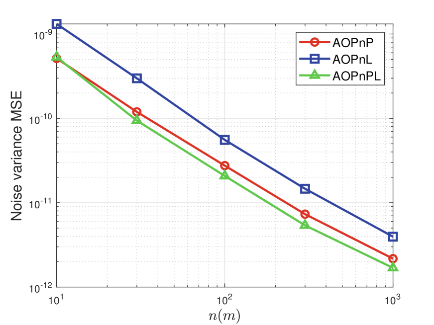
(a) $\sigma=5$ pixels

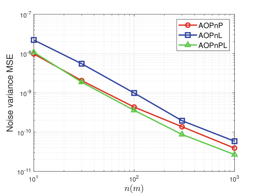
(b) $\sigma=10$ pixels

Figure 4: MSEs of noise variance estimates.

(2) Asymptotic unbiasedness of pose estimators. As stated before, in (16), (20), and (23), the regressor is correlated with the noise term. Without bias elimination, the estimates derived from these equations are not asymptotically unbiased. Based on the estimate of noise variance, the proposed bias elimination method can eliminate the asymptotic bias. These claims are verified in Figure 5, where we use “w.o.” and “BE” for the abbreviations of “without” and “bias elimination”, respectively. Without bias elimination, the biases of the estimators converge to a nonzero value, although the PnPL estimator achieves a much smaller bias compared to the PnP and PnL estimators. The biases of the proposed bias-eliminated estimators all converge to $0$, implying that they are asymptotically unbiased.

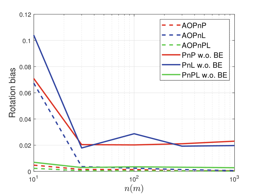
(a) $\sigma=5$ pixels ($\bf R$)

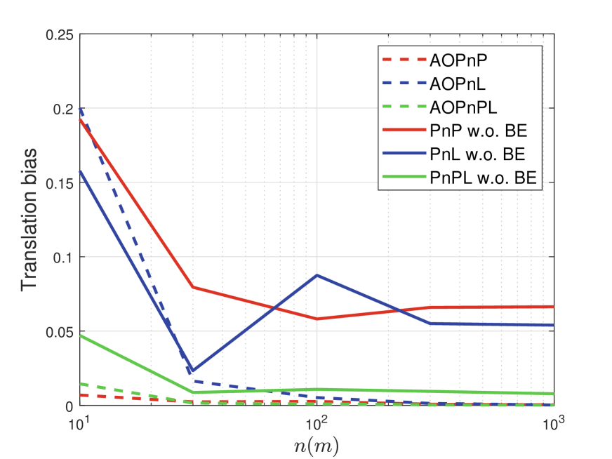
(b) $\sigma=5$ pixels ($\bf t$)

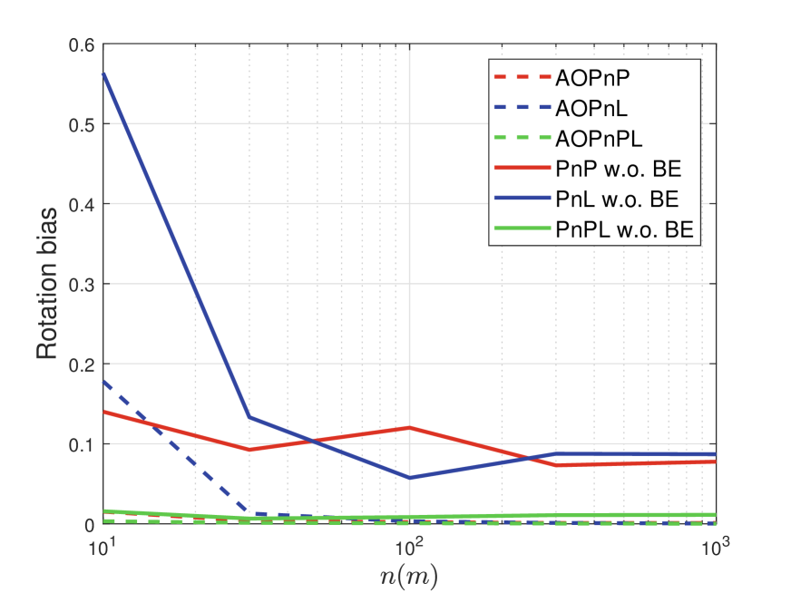
(c) $\sigma=10$ pixels ($\bf R$)

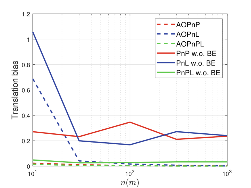
(d) $\sigma=10$ pixels ($\bf t$)

Figure 5: Biases of pose estimates.

(3) Consistency and asymptotic efficiency of pose estimators. We have proved that the proposed estimator is $\sqrt{n+m}$-consistent in its first step, based on which a single GN iteration suffices to reach the CRB, i.e., the proposed two-step estimator is asymptotically efficient. The MSE comparison among different PnP pose estimators is presented in Figure 6. It is obvious from Figure 6(d) that the MSEs of the DLS, EPnP, and SQPnP estimators do not converge to $0$. This is because they are not asymptotically unbiased, and their asymptotic MSEs are dominated by asymptotic biases. We can see that when $n\geq 30$, our estimator AOPnP can reach the CRB, coinciding with our theoretical claims. The CRB converges to $0$, which shows that the more point correspondences, the more accurate the estimate is. It is noteworthy that the MLPnP estimator seems to be also asymptotically efficient. This is because it performs multiple GN iterations. The attraction neighborhood of the global minimum of (13) is relatively large in this scenario. As a result, although the initial value is not consistent, it can still fall into the attraction neighborhood, and multiple GN iterations can find the global minimum. In Appendix E, we set $\sigma=50$ pixels. In this case, the initial value of the MLPnP falls beyond the attraction neighborhood, and the MLPnP estimate cannot reach the CRB.

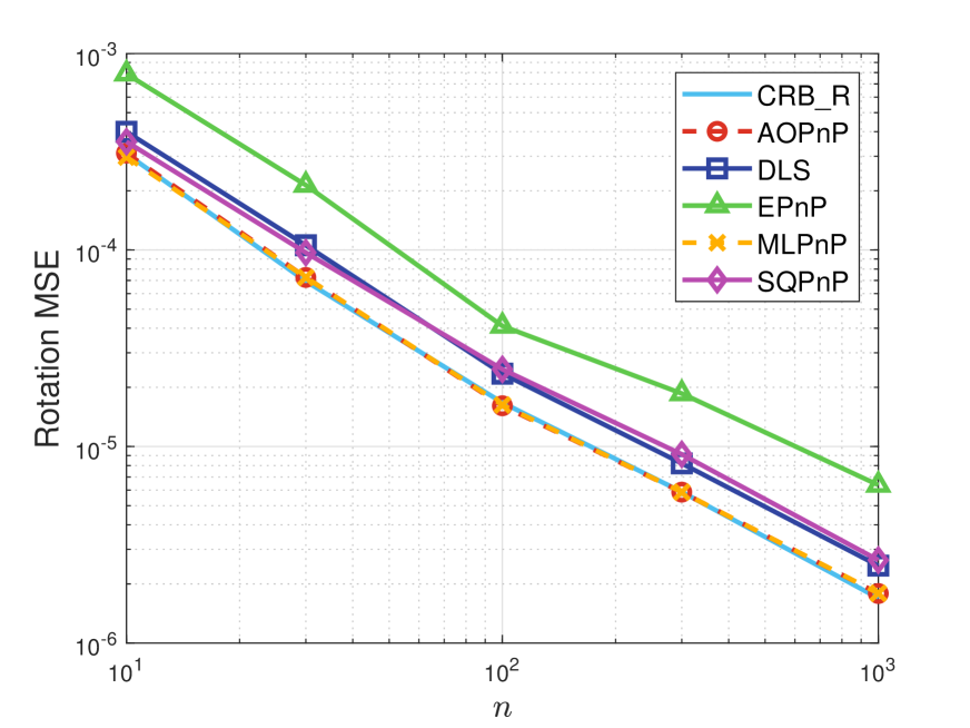
(a) $\sigma=5$ pixels ($\bf R$)

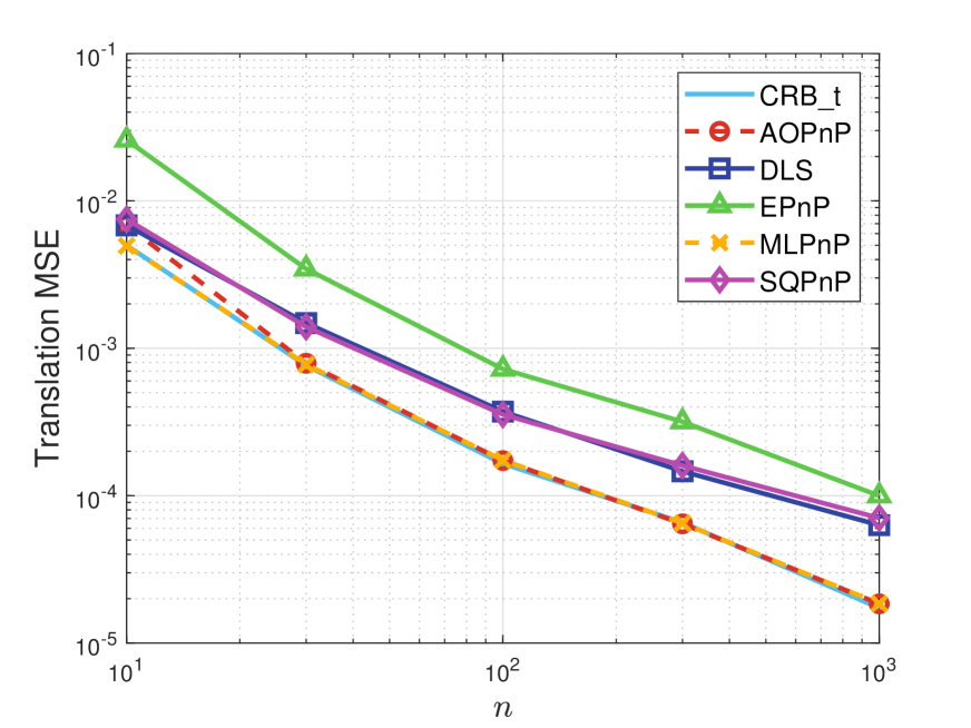
(b) $\sigma=5$ pixels ($\bf t$)

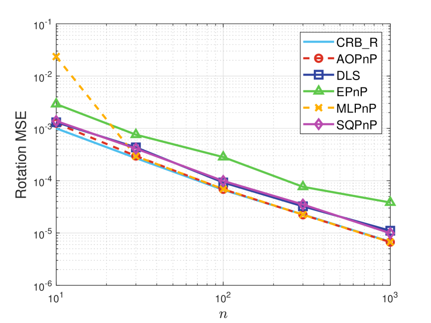
(c) $\sigma=10$ pixels ($\bf R$)

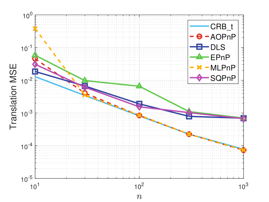
(d) $\sigma=10$ pixels ($\bf t$)

Figure 6: MSEs of PnP pose estimates.

The MSE comparison among different PnL pose estimators is presented in Figure 7. We see that the proposed AOPnL estimator can asymptotically reach the CRB. In addition, it outperforms the other estimators significantly. It seems that the compared PnL estimators are less stable than previous PnP estimators. When $\sigma=10$ pixels, the MSEs of the ASPnL, SRPnL, and AlgLS estimators fluctuate w.r.t. the line number.

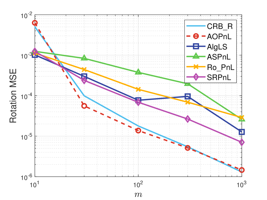
(a) $\sigma=5$ pixels ($\bf R$)

(b) $\sigma=5$ pixels ($\bf t$)

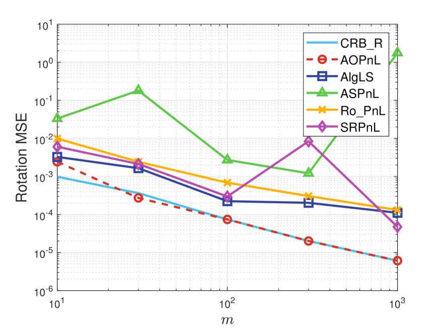
(c) $\sigma=10$ pixels ($\bf R$)

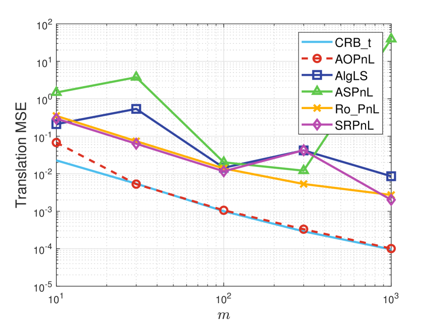
(d) $\sigma=10$ pixels ($\bf t$)

Figure 7: MSEs of PnL pose estimates.

Finally, we compare different PnPL estimators which utilize both point and line correspondences. The result is shown in Figure 8. The proposed estimator AOPnPL can asymptotically reach the CRB. It is noteworthy that when the measurement number is relatively small, the AOPnPL estimator may outperform the CRB. This is because the CRB is a lower bound for unbiased estimators, while the proposed estimator is not necessarily unbiased in a finite sample case. For the comparison estimators, they are less accurate than ours. Especially in the case of a large measurement number and noise intensity, the proposed AOPnPL can outperform the other estimators more than 10 times.

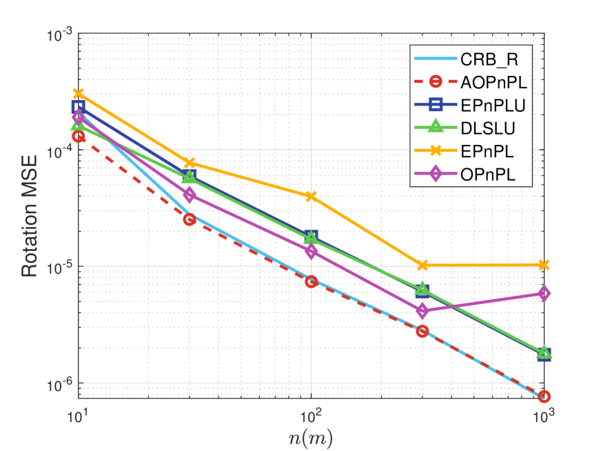
(a) $\sigma=5$ pixels ($\bf R$)

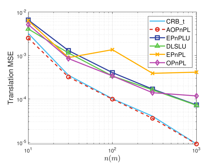
(b) $\sigma=5$ pixels ($\bf t$)

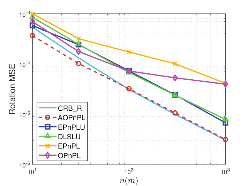
(c) $\sigma=10$ pixels ($\bf R$)

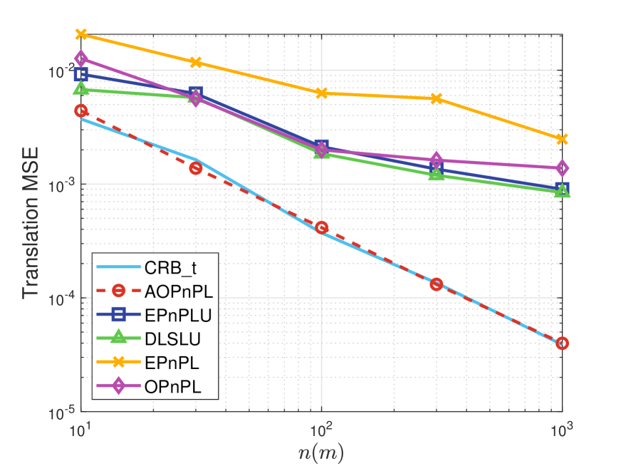
(d) $\sigma=10$ pixels ($\bf t$)

Figure 8: MSEs of PnPL pose estimates.

The MSE comparison of our proposed estimators using different kinds of measurements is shown in Figure 9. We see that using only point correspondences or only line correspondences leads to comparable MSEs. This is because the intensity of the noises added to points and endpoints of lines is the same, and each point or line correspondence yields two independent equations. By fusing point and line measurements, the AOPnPL estimator can achieve an MSE smaller than half of that of the AOPnP and AOPnL estimators.

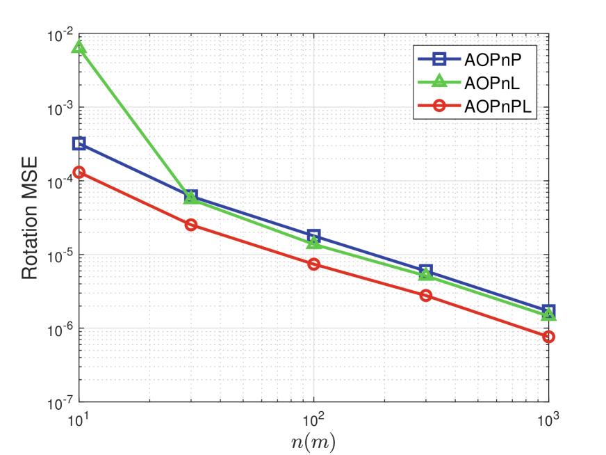
(a) $\sigma=5$ pixels ($\bf R$)

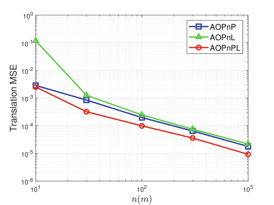
(b) $\sigma=5$ pixels ($\bf t$)

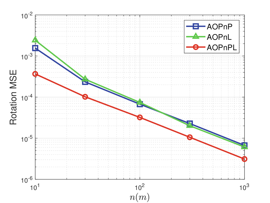
(c) $\sigma=10$ pixels ($\bf R$)

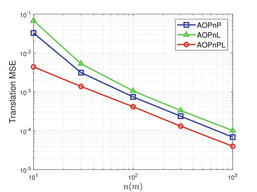
(d) $\sigma=10$ pixels ($\bf t$)

Figure 9: MSEs of different kinds of measurements.

(4) Linear time complexity of pose estimators. Since the solution in the first step can be calculated analytically, and only a single GN iteration is performed in the second step, the total time complexity of our algorithm is $O(n+m)$, i.e., the cost time increases linearly w.r.t. the measurement number. The accumulated CPU time (over $1000$ Monte Carlo tests) of all tested algorithms is presented in Figure 10. Apart from the SQPnP using Python implementation, all algorithms are executed with MATLAB codes. We see that the CPU time of our proposed algorithm increases linearly w.r.t. the measurement number. Among all tested algorithms, our proposed one is at an intermediate level. Some estimators, such as Ro_PnL and ASPnL, may be unable to be implemented in real time when the measurement number is large.

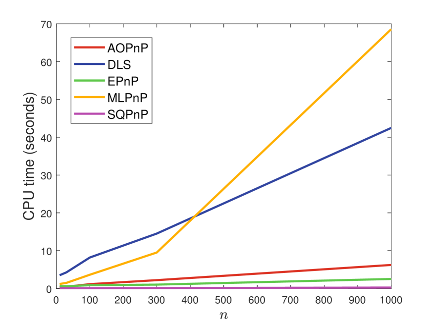
(a) PnP estimators

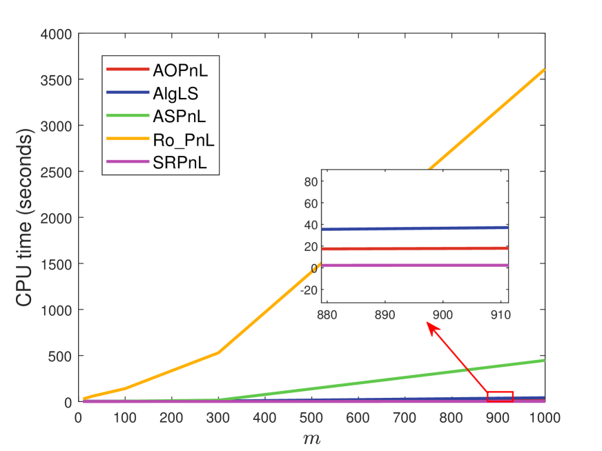
(b) PnL estimators

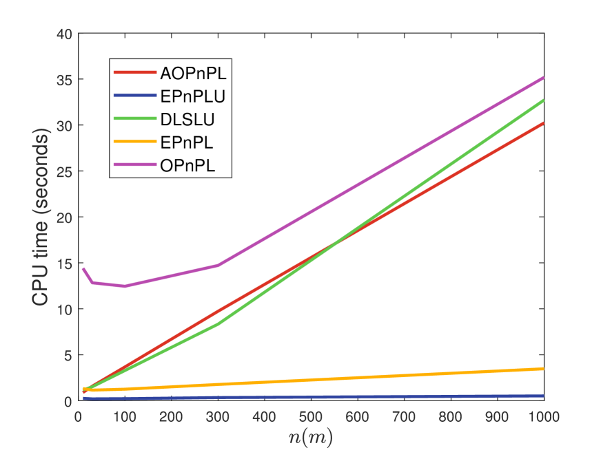
(c) PnPL estimators

(d) Different estimators

Figure 10: Accumulated CPU time comparison over $1000$ Monte Carlo tests.

7.2 Static real image tests

In this subsection, we conduct static real image tests, which correspond to the applications of absolute robot pose estimation in a pre-reconstructed map. First, we compare PnP estimators with the ETH3D dataset [41]. The dataset has $13$ scenes, each of which contains dozens of images. Figure 11 gives the mean estimation errors of PnP estimators in all scenes. In most scenes, our estimator AOPnP achieves the smallest errors. Resembling the simulation, the MLPnP algorithm owns a comparable accuracy with AOPnP, while the other estimators have much larger estimation errors.

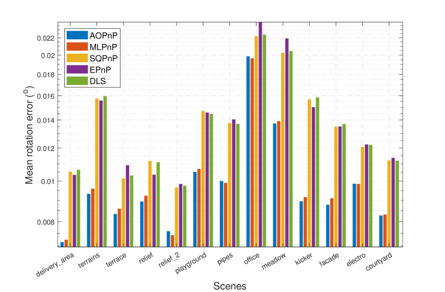
(a) Rotation errors

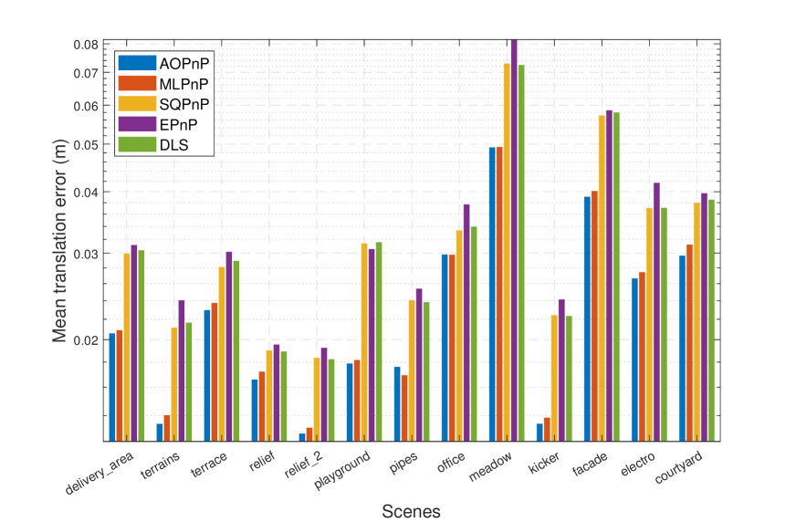
(b) Translation errors

Figure 11: Mean PnP pose estimation error comparison in $13$ scenes of the ETH3D dataset.

We select four scenes where our estimator has the smallest mean errors and plot the error distribution in Figure 12. We find that the reason why the AOPnP estimator performs best is two-fold: First, it produces less severe outlier estimates; Second, it has lower quartiles.

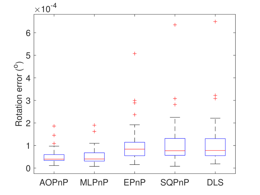
(a) Delivery area ($\bf R$)

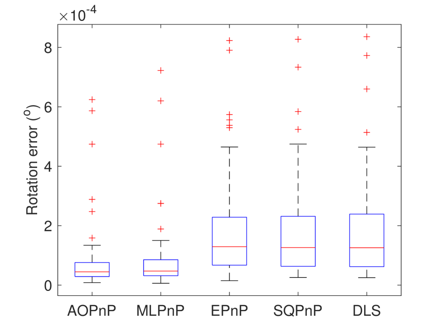
(b) Facade ($\bf R$)

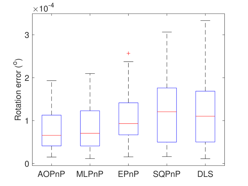
(c) Relief ($\bf R$)

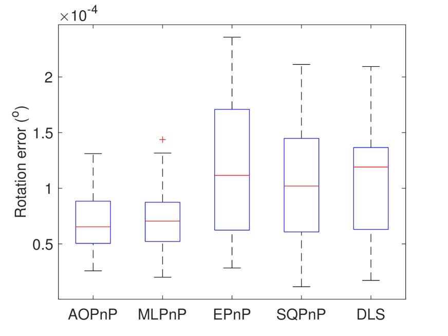
(d) Terrace ($\bf R$)

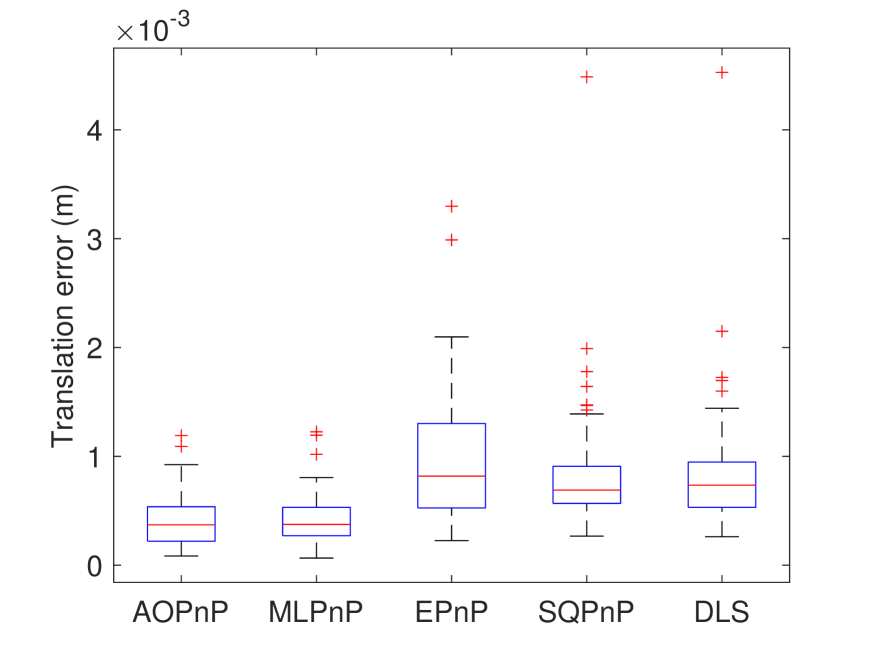
(e) Delivery area ($\bf t$)

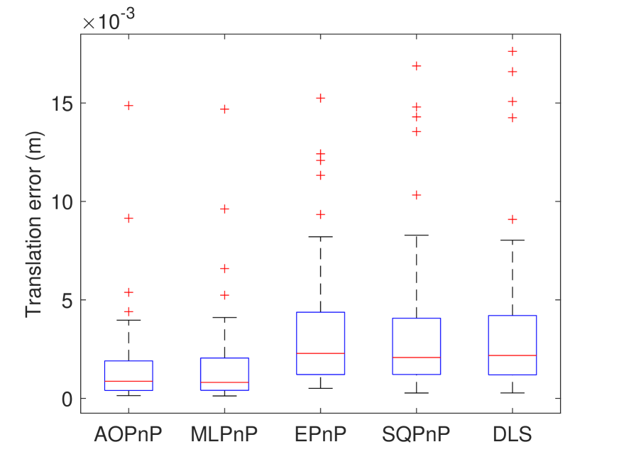
(f) Facade ($\bf t$)

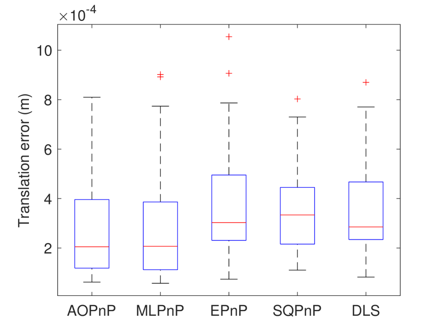
(g) Relief ($\bf t$)

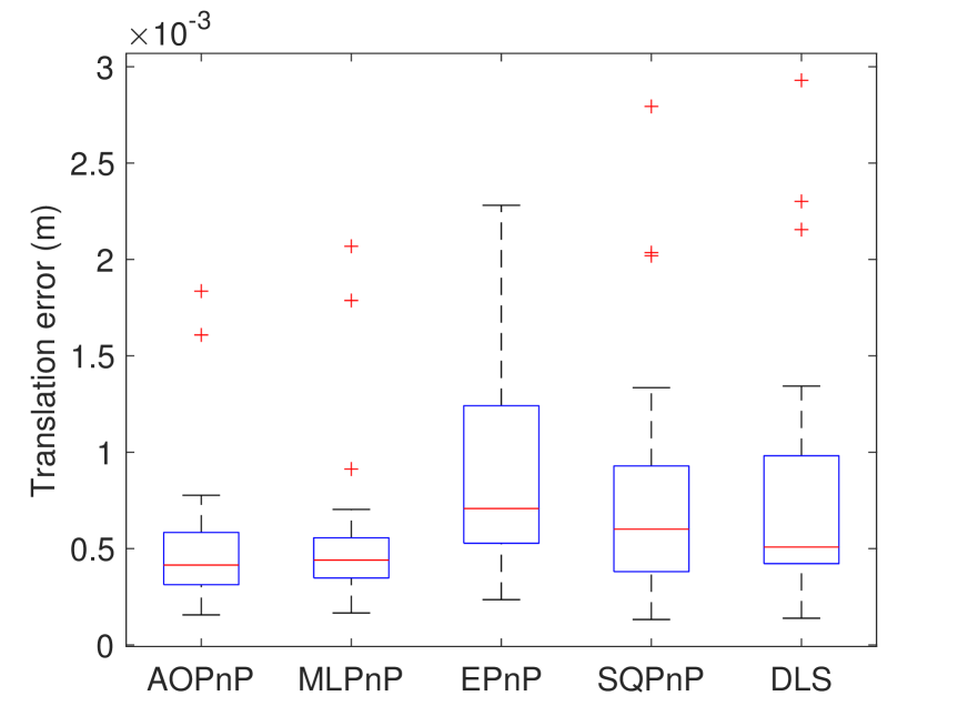
(h) Terrace ($\bf t$)

Figure 12: Error distribution of the scenes of delivery area, facade, relief, and terrace.

To test the relationship between the MSEs and point number $n$, we randomly select four images that have abundant point correspondences. In each trial, we randomly select a certain number of points to infer the camera pose, and the MSEs are calculated by $100$ Monte Carlo trials. The result is plotted in Figure 13. We see that the MSE of our AOPnP solver consistently declines as $n$ increases. Moreover, it significantly outperforms the EPnP, DLS, and SQPnP estimators when $n$ is relatively large. Although the MLPnP estimator has a similar MSE to AOPnP, noting that it has high time complexity, our algorithm performs best by taking both accuracy and efficiency into account.

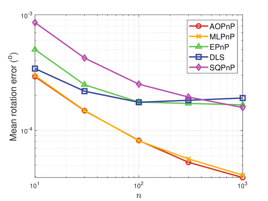
(a) Facade 14 ($\bf R$)

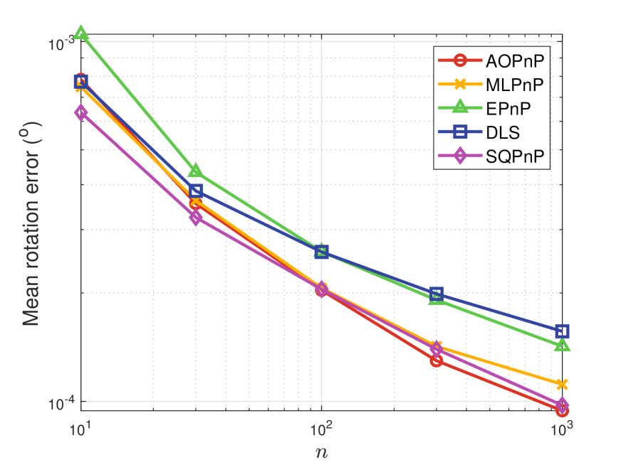
(b) Kicker 26 ($\bf R$)

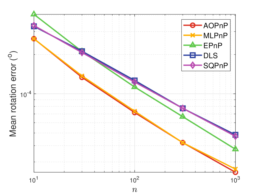
(c) Delivery area 10 ($\bf R$)

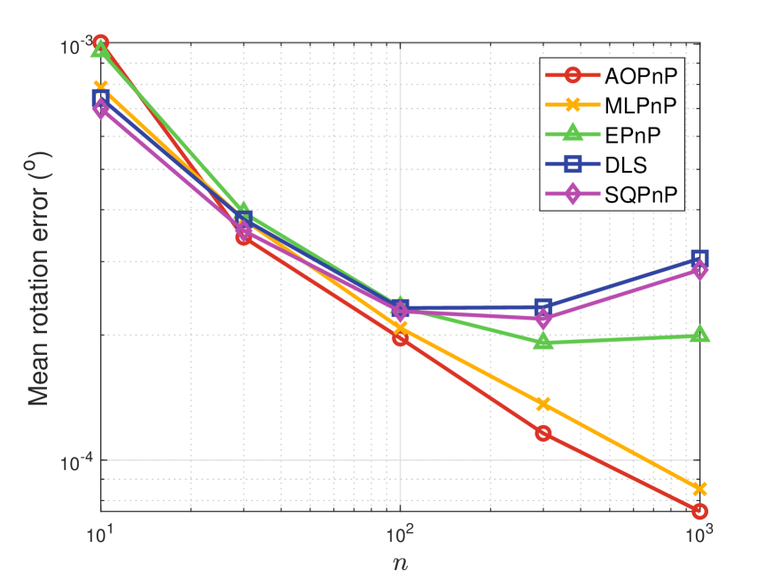
(d) Terrains 41 ($\bf R$)

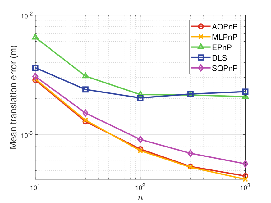
(e) Facade 14 ($\bf t$)

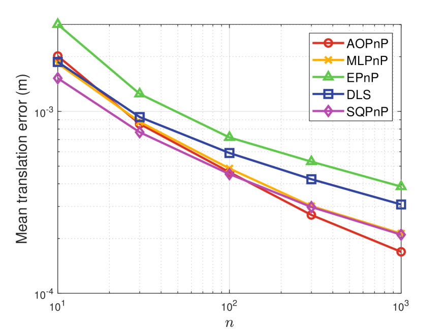
(f) Kicker 26 ($\bf t$)

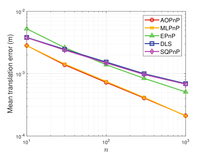
(g) Delivery area 10 ($\bf t$)

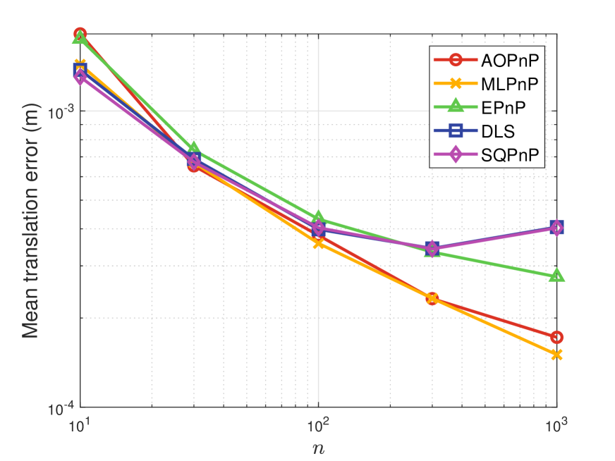
(h) Terrains 41 ($\bf t$)

Figure 13: Consistency test of four images with abundant point features. “Facade 14” means the fourteenth image in the facade scene.

Second, we compare PnL estimators with the VGG dataset [42]. Figure 14 presents the mean estimation errors of PnL estimators in the tested scenes. Our estimator AOPnL achieves the smallest errors except for the Model House scene. Moreover, the magnitude of superiority is significant and sometimes can reach $3$ orders. The reason why AOPnL has large average errors in the Model House scene is that there are two images with relatively few lines and AOPnL produces abnormal pose estimates. Since each scene only contains several images, we do not plot the corresponding error distribution.

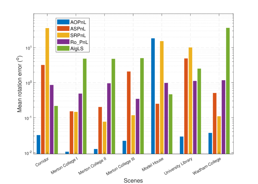
(a) Rotation errors

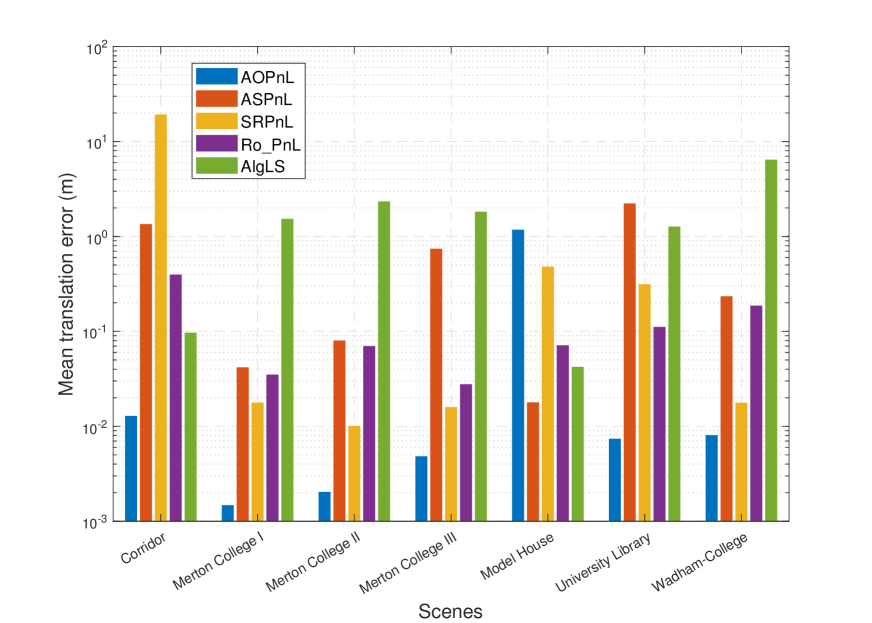
(b) Translation errors

Figure 14: Mean PnL pose estimation error comparison in $7$ scenes of the VGG dataset.

We select four images and reproject 3D lines onto the images using estimated poses to show the estimation precision qualitatively. As shown in Figure 15, with the estimated poses by our estimator, the projected lines coincide with the given 2D lines well, whereas the other estimators generate deviated lines, especially the Ro_PnL and ASPnL methods with lines in the sky or on the grass. The result of the AlgLS estimator is omitted because its estimation errors are too large and the lines cannot be displayed in the images.

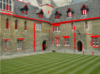
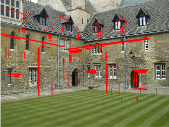
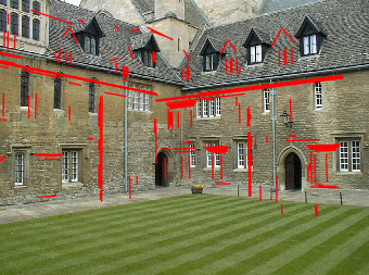
AOPnL Ro_PnL ASPnL SRPnL

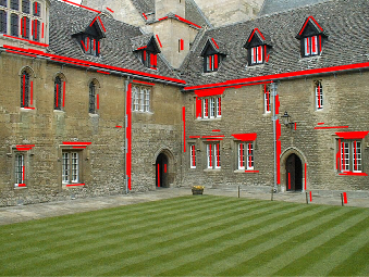
Merton-College-I

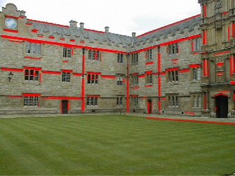
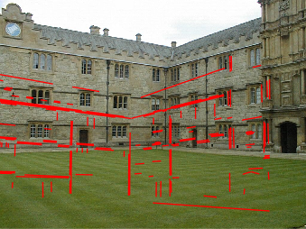
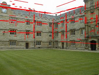
Merton-College-II

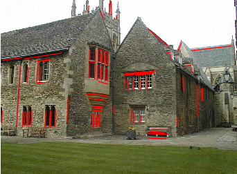
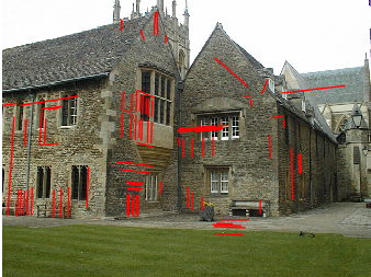
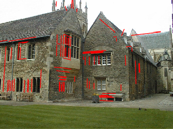
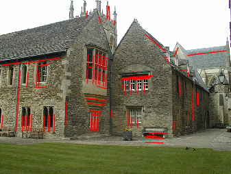
Merton-College-III

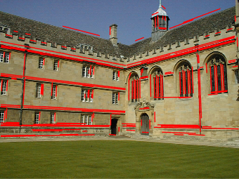
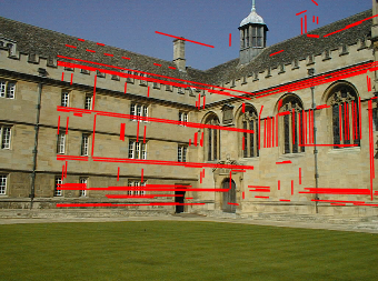
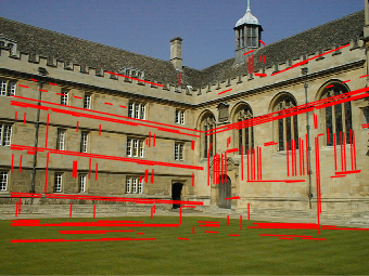
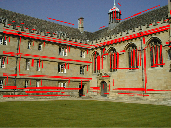
Wadham-College

Figure 15: Line reprojection onto images with estimated poses.

We use the four images in Figure 15 to test the relationship between the MSEs and line number $m$. In each trial, we randomly select a certain number of lines to infer the camera pose, and the MSEs are calculated by $100$ Monte Carlo trials. The result is plotted in Figure 16. The MSE of our AOPnL solver declines as $m$ increases. In addition, it is much smaller than that of the other methods. The Ro_PnL and SRPnL estimators seem not so stable and the AlgLS estimator has the largest MSE.

(a) Merton I ($\bf R$)

(b) Merton II ($\bf R$)

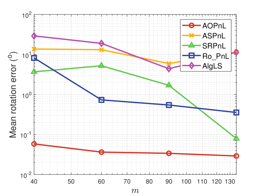
(c) Merton III ($\bf R$)

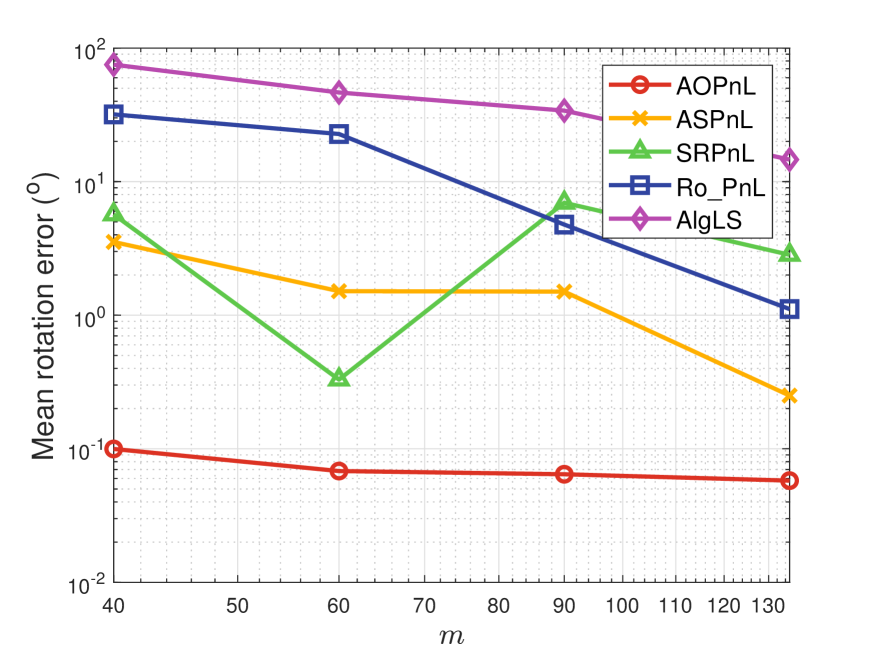
(d) Wadham ($\bf R$)

(e) Merton I ($\bf t$)

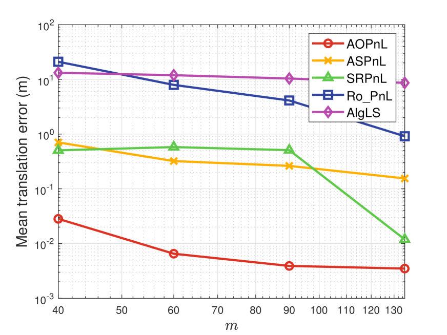
(f) Merton II ($\bf t$)

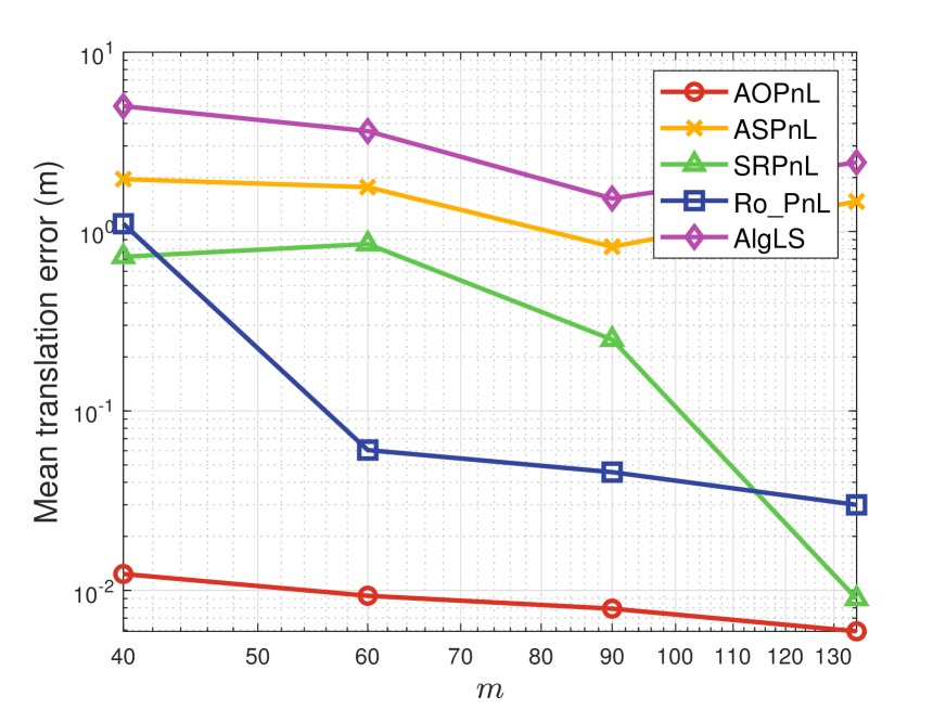
(g) Merton III ($\bf t$)

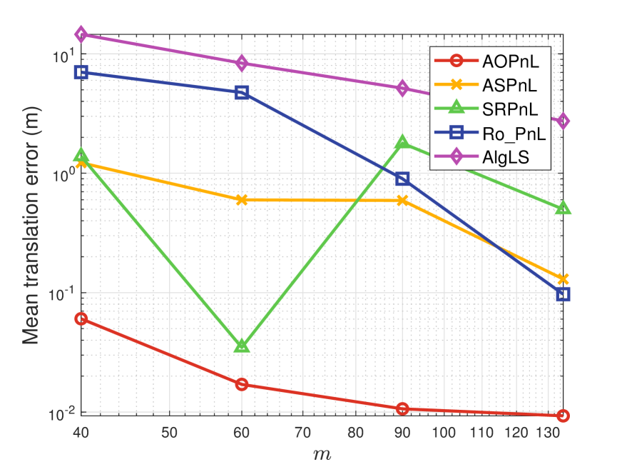
(h) Wadham ($\bf t$)

Figure 16: Consistency test of four images with abundant line features.

Finally, we compare PnPL estimators with the VGG dataset. Figure 17 presents the mean estimation errors of PnPL estimators in the tested scenes. In practice, we find that the noise variances of points and lines can be quite different, hence we estimate them separately. Note that the EPnPLU and DLSU estimators need extra prior information about uncertainties of 2D projections and the average scene depth. We use the true scene depth and our estimated noise variance as their inputs. We see that the proposed AOPnL estimator performs best, especially for the estimation of orientation. Even though the EPnPLU and DLSU methods utilize the true depth scene, our estimator has better accuracy.

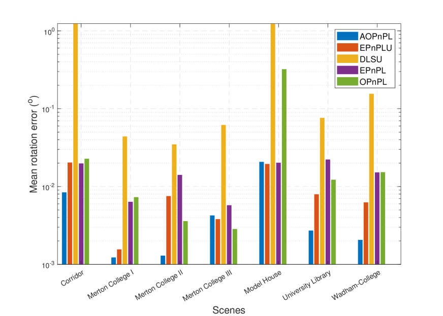
(a) Rotation errors

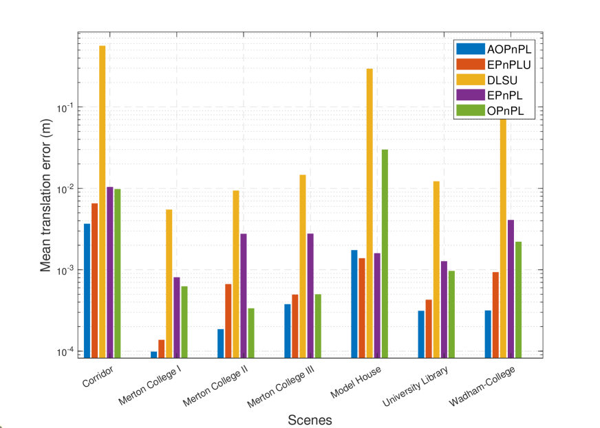
(b) Translation errors

Figure 17: Mean PnPL pose estimation error comparison in $7$ scenes of the VGG dataset.

7.3 Visual odometry with real image sequences

In the last subsection, we have tested the static camera pose estimation which corresponds to robot localization in a known 3D map. A more common scenario is that a robot explores and navigates in an unknown environment, which involves SLAM or odometry. In this subsection, we embed PnP estimators into a stereo visual odometry pipeline and compare the accuracy and efficiency using the EuRoC MAV dataset [50]. The odometry mainly includes three components: feature extraction and tracking, triangulation, and PnP solver. Harris corners are extracted on the left image first, and then their correspondences on the right image are found by Lucas-Kanade (L-K) optical flow. To reject outliers, inverse L-K optical flow is employed. Feature tracking is only performed on the left camera, which is also done by L-K optical flow. Fundamental-matrix-based RANSAC is adopted to improve the quality of point correspondences. Once the correspondences are established, the depth of feature points can be obtained by triangulation, using the extrinsics between stereo cameras. The points tracked on the left camera can be triangulated based on the relative pose given by the previous estimation. With the triangulated 3D points and their 2D correspondences, we utilize iterative-PnP-based RANSAC to filter outliers. Finally, the inliers will be fed into a PnP algorithm to obtain the frame-to-frame pose estimation. The PnP solver would be replaced by different algorithms, while the other components remain unchanged.

We select four sequences labeled “easy” in the EuRoC dataset since they exhibit less dynamic motion, allowing the extraction of high-quality feature points and their correspondences. The maximum number of points extracted in one frame is limited to 1000, and the distance between every two points should be greater than 15 pixels, which can promote uniform distribution of features in the image. The extrinsics between stereo cameras are given by dataset defaults. All algorithms are run on an Intel-13500H mobile CPU upon WSL2 (Windows Subsystem Linux).

Figure 18 plots the real-time absolute pose error (APE) at each instant, and Table 1 gives the APE RMSE where “/” represents that the corresponding PnP algorithm fails to generate a reasonable odometry. Other than the MH01 sequence, the proposed AOPnP algorithm consistently has the smallest APE RMSE, and the superiority is significant for the VR201 sequence. The APE RMSE of AOPnP is slightly inferior to the MLPnP estimator in the MH01 sequence. It is noteworthy that the DLS and EPnP algorithms both fail in all sequences. This is because their pose estimation precision is relatively low and the accumulated drift rapidly increases to an abnormal value. The instantaneous APE figure supports the RMSE result. The estimated trajectory is plotted in Figure 19. Overall, the trajectory based on AOPnP coincides with the ground truth best, especially in the VR201 sequence. The MLPnP algorithm has a comparable performance with the proposed one in the other three sequences, which is better than the SQPnP algorithm.

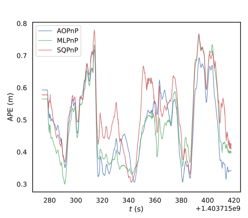
(a) VR101

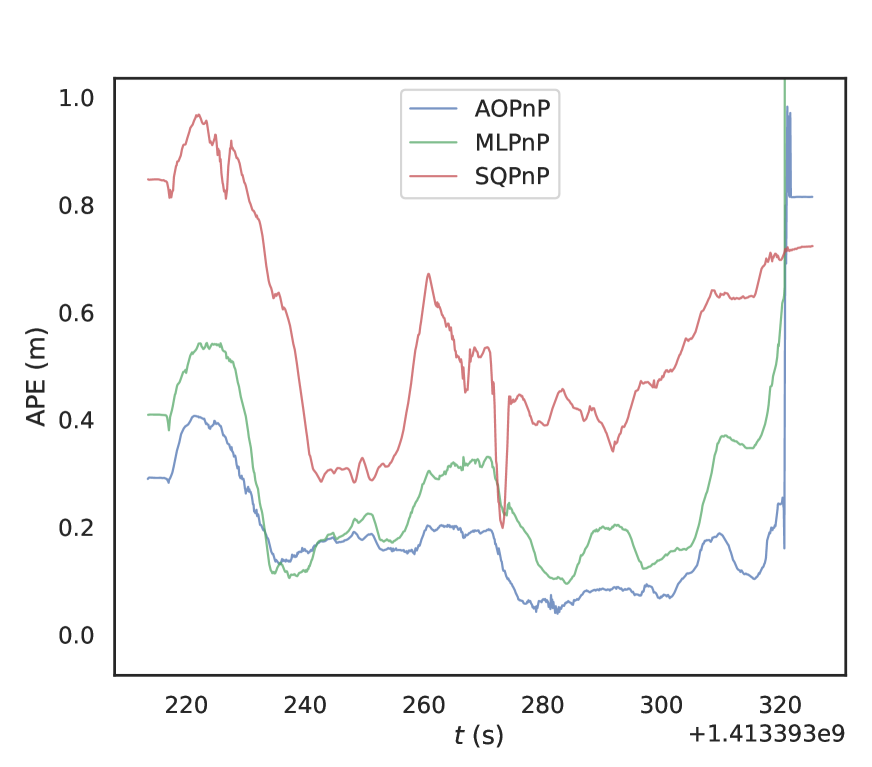
(b) VR201

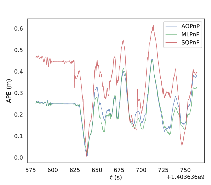
(c) MH01

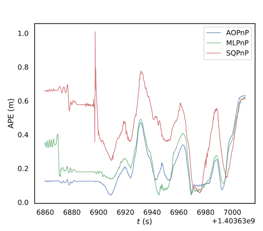
(d) MH02

Figure 18: Real-time APE in stereo visual odometry evaluation.

Table 1: APE RMSE w.r.t. the translation part (unit: m) in stereo visual odometry evaluation.

	AOPnP	DLS	EPnP	MLPnP	SQPnP
VR101	0.49491	/	/	0.49492	0.5393
VR201	0.2535	/	/	0.5226	0.5863
MH01	0.2471	/	/	0.2349	0.3745
MH02	0.2363	/	/	0.2692	0.4903

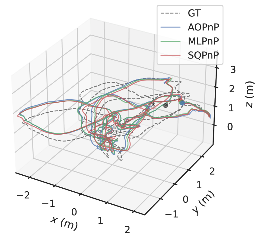
(a) VR101

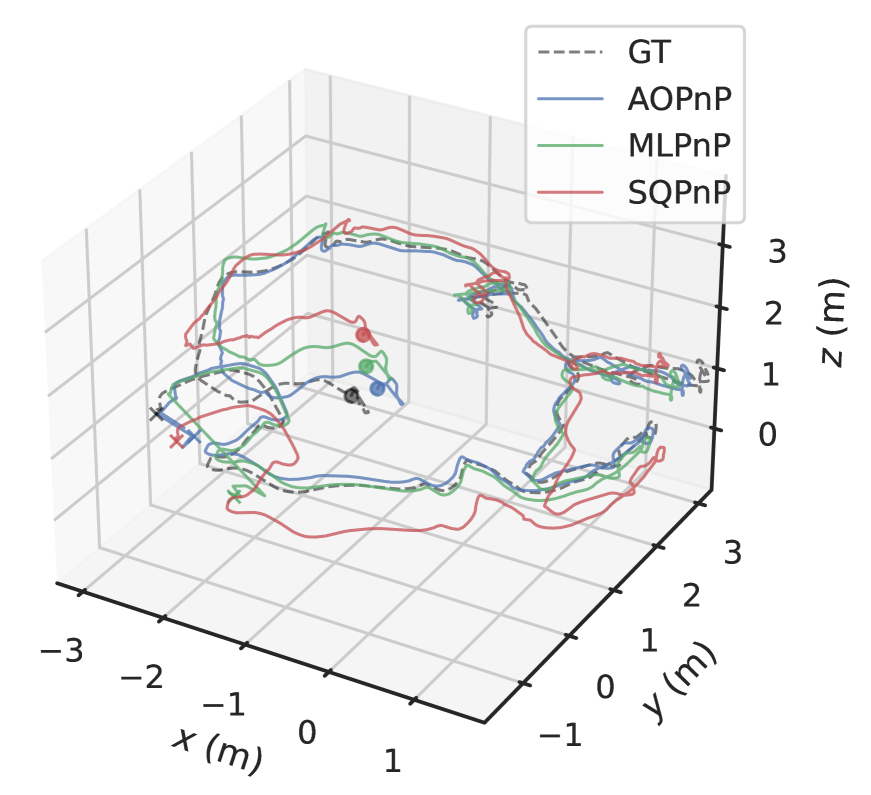
(b) VR201

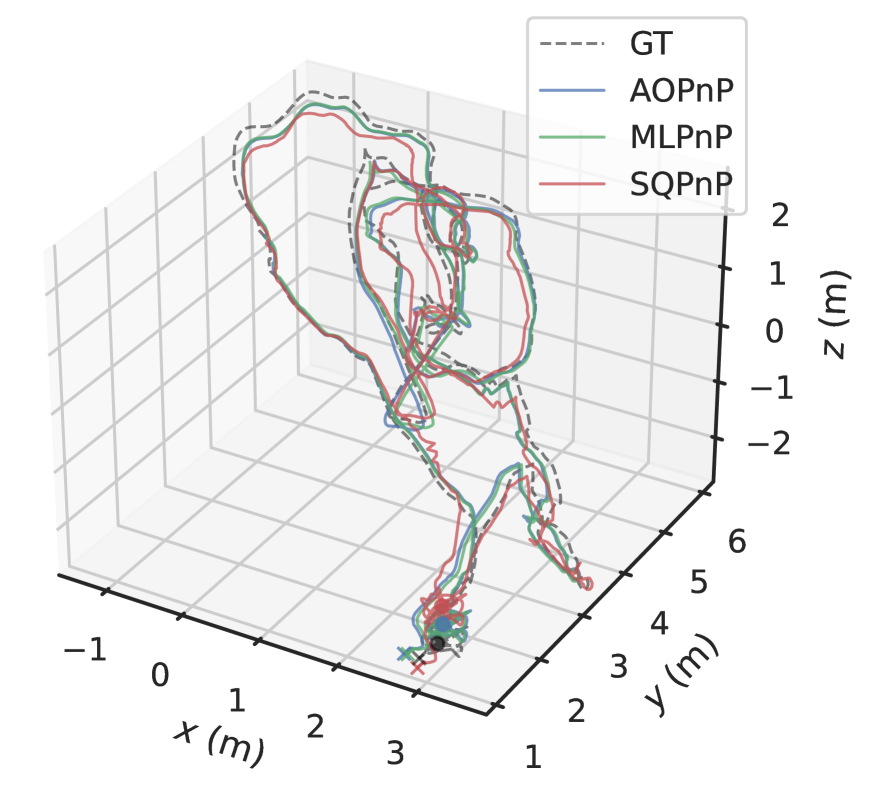
(c) MH01

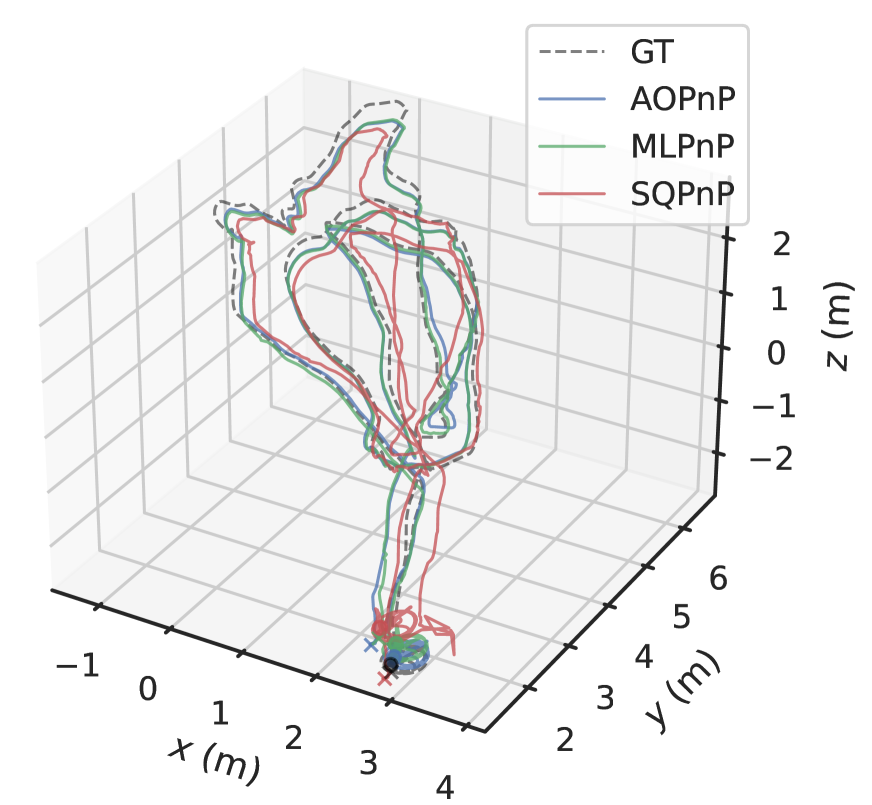
(d) MH02

Figure 19: Estimated trajectory in stereo visual odometry evaluation.

Table 2 lists the CPU time consumed by each PnP algorithm in the odometry process. The SQPnP algorithm owns the lowest time complexity since it invokes only a small number of local searches. Compared with MLPnP, the proposed AOPnP estimator is about four times faster, which can save time for other pipelines in a comprehensive SLAM or odometry system while maintaining a relatively high accuracy.

Table 2: CPU time (unit: s) in stereo visual odometry evaluation.

	AOPnP	MLPnP	SQPnP
VR101	0.321	1.258	0.089
VR201	0.281	1.176	0.080
MH01	0.399	1.499	0.101
MH02	0.617	2.215	0.239

In summary, in the dynamic odometry evaluation, our proposed AOPnP estimator features the best estimation accuracy while possessing a relatively low time complexity. When combined with a feature extraction and tracking module that can yield plenty of high-quality correspondences, it is well-suited for precision-demanding and real-time SLAM applications.

8 Conclusion and future work

In this paper, we proposed a uniform camera-robot pose estimation algorithm that can take points, lines, or combined points and lines as inputs. By virtue of noise variance estimation and bias elimination, the algorithm is asymptotically unbiased and consistent in the first step. Then, an ensuing single GN iteration in the second step makes the estimate to be asymptotically efficient. Thanks to the simple form in each step, our estimator scales linearly with respect to the feature number. Three kinds of experiments showed the advantages of the proposed algorithm in terms of estimation accuracy and time complexity. To fully unleash the potential of the proposed algorithm, it is desirable to equip it with a frontend that can extract and match a relatively large number of high-quality features.

In future work, a more concise pose parameterization method may be adopted to improve the estimation accuracy when the feature number is few while maintaining the properties of consistency and asymptotic efficiency. In addition, how to achieve consistency against outlier feature correspondences in some outlier-prone scenarios is also an interesting problem.

Appendix A Proof of Theorems 1 and 3

The proof is mainly based on the following lemma:

Lemma 2 ([49, Lemma 4]).

Let $\{X_{i}\}$ be a sequence of independent random variables with $\mathbb{E}[X_{i}]=0$ and $\mathbb{E}\left[X_{i}^{2}\right]\leq\varphi<\infty$ for all $i$. Then, there holds $\sum_{i=1}^{n}X_{i}/n=O_{p}(1/\sqrt{n})$.

To prove Theorem 1, let

$$\Delta{\bf A}_{n}\triangleq{\bf A}_{n}-{\bf A}_{n}^{o}=\begin{bmatrix}[{\bm{\epsilon}}_{{\bf x}_{1}}^{h\wedge}]_{1:2}\mkern 2.5mu\overline{\mkern-2.5mu\bf X\mkern-2.5mu}\mkern 2.5mu_{1}&[{\bm{\epsilon}}_{{\bf x}_{1}}^{h\wedge}]_{1:2}\\ \vdots&\vdots\\ [{\bm{\epsilon}}_{{\bf x}_{n}}^{h\wedge}]_{1:2}\mkern 2.5mu\overline{\mkern-2.5mu\bf X\mkern-2.5mu}\mkern 2.5mu_{n}&[{\bm{\epsilon}}_{{\bf x}_{n}}^{h\wedge}]_{1:2}\end{bmatrix}.$$

Then, we have

$${\bf Q}_{n}-{\bf Q}_{n}^{o} =\frac{1}{n}(\Delta{\bf A}_{n}^{\top}{\bf A}_{n}^{o}+{\bf A}_{n}^{o\top}\Delta{\bf A}_{n}+\Delta{\bf A}_{n}^{\top}\Delta{\bf A}_{n})$$

$$=\frac{1}{n}(\Delta{\bf A}_{n}^{\top}\Delta{\bf A}_{n})+O_{p}(1/\sqrt{n})$$

$$=\frac{\sigma^{2}}{n}(\tilde{\bf A}_{n}^{\top}\tilde{\bf A}_{n})+O_{p}(1/\sqrt{n})$$

$$=\hat{\sigma}^{2}_{n}\tilde{\bf Q}_{n}+O_{p}(1/\sqrt{n}),$$

where the second and third “$=$” are based on Lemma 2, and the last “$=$” attributes to the boundedness of $\tilde{\bf Q}_{n}$. Hence, (19) holds. For the other claim, note that (1). ${\bf Q}_{n}^{\rm BE}$ converges to ${\bf Q}_{n}^{o}$ with a rate of $1/\sqrt{n}$; (2). eigenvectors are continuously changing w.r.t. the varying of a matrix; (3). $\bar{\bm{\theta}}^{o}$ is a unit vector corresponding to the smallest eigenvalue of ${\bf Q}_{n}^{o}$. Therefore, $\hat{\bm{\theta}}^{\rm BE}_{n}$ is a $\sqrt{n}$-consistent estimate of $\bar{\bm{\theta}}^{o}$ up to sign, which completes the proof.

To prove Theorem 3, let

$$\Delta{\bf A}_{m}\triangleq{\bf A}_{m}-{\bf A}_{m}^{o}=\begin{bmatrix}[{\bm{\epsilon}}_{{\bf p}_{1}}^{h}\leavevmode\nobreak\ {\bm{\epsilon}}_{{\bf q}_{1}}^{h}]^{\top}\mkern 2.5mu\overline{\mkern-2.5mu\bf L\mkern-2.5mu}\mkern 2.5mu_{1}\\ \vdots\\ [{\bm{\epsilon}}_{{\bf p}_{m}}^{h}\leavevmode\nobreak\ {\bm{\epsilon}}_{{\bf q}_{m}}^{h}]^{\top}\mkern 2.5mu\overline{\mkern-2.5mu\bf L\mkern-2.5mu}\mkern 2.5mu_{m}\end{bmatrix}.$$

Then, we have

$${\bf Q}_{m}-{\bf Q}_{m}^{o} =\frac{1}{m}(\Delta{\bf A}_{m}^{\top}{\bf A}_{m}^{o}+{\bf A}_{m}^{o\top}\Delta{\bf A}_{m}+\Delta{\bf A}_{m}^{\top}\Delta{\bf A}_{m})$$

$$=\frac{1}{m}(\Delta{\bf A}_{m}^{\top}\Delta{\bf A}_{m})+O_{p}(1/\sqrt{m})$$

$$=\frac{\sigma^{2}}{m}(\tilde{\bf A}_{m1}^{\top}\tilde{\bf A}_{m1}+\tilde{\bf A}_{m2}^{\top}\tilde{\bf A}_{m2})+O_{p}(1/\sqrt{m})$$

$$=\hat{\sigma}^{2}_{m}(\tilde{\bf Q}_{m1}+\tilde{\bf Q}_{m2})+O_{p}(1/\sqrt{m}),$$

where the second and third “$=$” are based on Lemma 2, and the last “$=$” attributes to the boundedness of $\tilde{\bf Q}_{m1}$ and $\tilde{\bf Q}_{m2}$. Hence, (22) holds. The other claim can be verified similarly to the point case and is omitted here.

Appendix B Derivatives in the GN iteration

Let

$${\bf r}_{pi}^{\rm den}({\bf s},{\bf t}) \triangleq{\bf e}_{3}^{\top}(\hat{\bf R}^{\rm BE}{\rm exp}({\bf s}^{\wedge}){\bf X}_{i}+{\bf t}),$$

$${\bf r}_{pi}^{\rm num}({\bf s},{\bf t}) \triangleq{\bf E}(\hat{\bf R}^{\rm BE}{\rm exp}({\bf s}^{\wedge}){\bf X}_{i}+{\bf t}).$$

Then, we have

$$\frac{\partial{\bf r}_{pi}}{\partial{\bf s}^{\top}}\big{\rvert}_{{\bf s}=0} =\frac{\left({\bf r}_{pi}^{\rm num}(0,{\bf t}){\bf e}_{3}^{\top}-{\bf r}_{pi}^{\rm den}(0,{\bf t}){\bf E}\right)({\bf X}_{i}^{\top}\otimes\hat{\bf R}^{\rm BE}){\bm{\Psi}}}{{\bf r}_{pi}^{\rm den}(0,{\bf t})^{2}},$$

$$\frac{\partial{\bf r}_{pi}}{\partial{\bf t}^{\top}}\big{\rvert}_{{\bf s}=0} =\frac{{\bf r}_{pi}^{\rm num}(0,{\bf t}){\bf e}_{3}^{\top}-{\bf r}_{pi}^{\rm den}(0,{\bf t}){\bf E}}{{\bf r}_{pi}^{\rm den}(0,{\bf t})^{2}},$$

where

$${\bm{\Psi}}\triangleq\frac{\partial{\rm vec}(\exp(\bf s^{\wedge}))}{\partial{\bf s}^{\top}}\Big{\rvert}_{\bf s=0}.$$

Note that ${\bm{\Sigma}}_{j}^{-\frac{1}{2}}{\bf r}_{lj}=[[{\bf r}_{lj}]_{1}/\sigma_{j}\leavevmode\nobreak\ \leavevmode\nobreak\ [{\bf r}_{lj}]_{2}/\sigma_{j}]^{\top}$, where $\sigma_{j}=\sigma\|[\bar{\bf l}_{j}]_{1:2}\|$. We have

$$\frac{\partial{\bm{\Sigma}}_{j}^{-\frac{1}{2}}{\bf r}_{lj}}{\partial{\bf s}^{\top}}\big{\rvert}_{{\bf s}=0} =\begin{bmatrix}\frac{1}{\sigma_{j}}&0\\ 0&\frac{1}{\sigma_{j}}\end{bmatrix}\frac{\partial{\bf r}_{lj}}{\partial{\bf s}^{\top}}\big{\rvert}_{{\bf s}=0}+{\rm diag}({\bf r}_{lj})\begin{bmatrix}\frac{\partial 1/\sigma_{j}}{\partial{\bf s}^{\top}}\big{\rvert}_{{\bf s}=0}\\ \frac{\partial 1/\sigma_{j}}{\partial{\bf s}^{\top}}\big{\rvert}_{{\bf s}=0}\end{bmatrix},$$

$$\frac{\partial{\bm{\Sigma}}_{j}^{-\frac{1}{2}}{\bf r}_{lj}}{\partial{\bf t}^{\top}}\big{\rvert}_{{\bf s}=0} =\begin{bmatrix}\frac{1}{\sigma_{j}}&0\\ 0&\frac{1}{\sigma_{j}}\end{bmatrix}\frac{\partial{\bf r}_{lj}}{\partial{\bf t}^{\top}}\big{\rvert}_{{\bf s}=0}+{\rm diag}({\bf r}_{lj})\begin{bmatrix}\frac{\partial 1/\sigma_{j}}{\partial{\bf t}^{\top}}\big{\rvert}_{{\bf s}=0}\\ \frac{\partial 1/\sigma_{j}}{\partial{\bf t}^{\top}}\big{\rvert}_{{\bf s}=0}\end{bmatrix}.$$

Let $\mkern 2.5mu\overline{\mkern-2.5mu\bf L\mkern-2.5mu}\mkern 2.5mu_{j1}\triangleq[{\bf L}_{j}]_{1:3}^{\top}\otimes{\bf I}_{3}$ and $\mkern 2.5mu\overline{\mkern-2.5mu\bf L\mkern-2.5mu}\mkern 2.5mu_{j2}\triangleq[{\bf L}_{j}]_{4:6}^{\top}\otimes{\bf I}_{3}$. We obtain

$$\frac{\partial{\bf r}_{lj}}{\partial{\bf s}^{\top}}\big{\rvert}_{{\bf s}=0} =[{\bf p}_{j}^{h}\leavevmode\nobreak\ {\bf q}_{j}^{h}]^{\top}\left(\mkern 2.5mu\overline{\mkern-2.5mu\bf L\mkern-2.5mu}\mkern 2.5mu_{j1}+{\bf t}^{\wedge}\mkern 2.5mu\overline{\mkern-2.5mu\bf L\mkern-2.5mu}\mkern 2.5mu_{j2}\right)({\bf I}_{3}\otimes\hat{\bf R}^{\rm BE}){\bm{\Psi}},$$

$$\frac{\partial{\bf r}_{lj}}{\partial{\bf t}^{\top}}\big{\rvert}_{{\bf s}=0} =-[{\bf p}_{j}^{h}\leavevmode\nobreak\ {\bf q}_{j}^{h}]^{\top}\left(\hat{\bf R}^{\rm BE}[{\bf L}_{j}]_{4:6}\right)^{\wedge},$$

and

$$\frac{\partial 1/\sigma_{j}}{\partial{\bf s}^{\top}}\big{\rvert}_{{\bf s}=0} =\frac{-[\bar{\bf l}_{j}]_{1:2}^{\top}\left[\left(\mkern 2.5mu\overline{\mkern-2.5mu\bf L\mkern-2.5mu}\mkern 2.5mu_{j1}+{\bf t}^{\wedge}\mkern 2.5mu\overline{\mkern-2.5mu\bf L\mkern-2.5mu}\mkern 2.5mu_{j2}\right)({\bf I}_{3}\otimes\hat{\bf R}^{\rm BE}){\bm{\Psi}}\right]_{1:2}}{\sigma\|[\bar{\bf l}_{j}]_{1:2}\|^{3}},$$

$$\frac{\partial 1/\sigma_{j}}{\partial{\bf t}^{\top}}\big{\rvert}_{{\bf s}=0} =\frac{[\bar{\bf l}_{j}]_{1:2}^{\top}\left[\left(\hat{\bf R}^{\rm BE}[{\bf L}_{j}]_{4:6}\right)^{\wedge}\right]_{1:2}}{\sigma\|[\bar{\bf l}_{j}]_{1:2}\|^{3}}.$$

Appendix C Proof of Theorem 7

Let $f({\bf s},{\bf t})$ denote the objective function of (13), where ${\bf R}=\hat{{\bf R}}^{\rm BE}\exp({\bf s}^{\wedge})$, and denote the optimal $\bf s$ and $\bf t$ as $\hat{\bf s}^{\rm ML}$ and $\hat{\bf t}^{\rm ML}$, respectively. Since $\hat{\bf R}^{\rm BE}$ and $\hat{\bf t}^{\rm BE}$ are $\sqrt{n+m}$-consistent, it holds that

$$\begin{bmatrix}\hat{\bf s}^{\rm ML}\\ \hat{\bf t}^{\rm ML}\end{bmatrix}-\begin{bmatrix}0\\ \hat{\bf t}^{\rm BE}\end{bmatrix}=O_{p}(1/\sqrt{n+m}).$$

Based on the optimality condition $\nabla f(\hat{\bf s}^{\rm ML},\hat{\bf t}^{\rm ML})=0$ and the Taylor expansion, we have

$$0=\nabla f(0,\hat{\bf t}^{\rm BE})+\nabla^{2}f(0,\hat{\bf t}^{\rm BE})\begin{bmatrix}\hat{\bf s}^{\rm ML}-0\\ \hat{\bf t}^{\rm ML}-\hat{\bf t}^{\rm BE}\end{bmatrix}+o_{p}(\frac{1}{\sqrt{n+m}}),$$

Then,

$$\begin{bmatrix}\hat{\bf s}^{\rm ML}-0\\ \hat{\bf t}^{\rm ML}-\hat{\bf t}^{\rm BE}\end{bmatrix}=-\nabla^{2}f(0,\hat{\bf t}^{\rm BE})^{-1}\nabla f(0,\hat{\bf t}^{\rm BE})+o_{p}(\frac{1}{\sqrt{n+m}}).$$ (28)

By combining (26) and (28), we finally obtain

$$\begin{bmatrix}\hat{\bf s}^{\rm ML}-\hat{\bf s}^{\rm GN}\\ \hat{\bf t}^{\rm ML}-\hat{\bf t}^{\rm GN}\end{bmatrix}$$

$$=\left({\bf J}^{\top}{\bf J}\right)^{-1}{\bf J}^{\top}{\bf r}-\nabla^{2}f(0,\hat{\bf t}^{\rm BE})^{-1}\nabla f(0,\hat{\bf t}^{\rm BE})+o_{p}(\frac{1}{\sqrt{n+m}})$$

$$=\left(\left(\frac{{\bf J}^{\top}{\bf J}}{n+m}\right)^{-1}-2\nabla^{2}f(0,\hat{\bf t}^{\rm BE})^{-1}\right)\frac{{\bf J}^{\top}{\bf r}}{n+m}+o_{p}(\frac{1}{\sqrt{n+m}})$$

$$=O_{p}(\frac{1}{\sqrt{n+m}})O_{p}(\frac{1}{\sqrt{n+m}})+o_{p}(\frac{1}{\sqrt{n+m}})$$

$$=o_{p}(\frac{1}{\sqrt{n+m}}),$$

where the second “$=$” is based on the fact that $\nabla f(0,\hat{\bf t}^{\rm BE})=\frac{2{\bf J}^{\top}{\bf r}}{n+m}$, and the third “$=$” is based on Lemma 2 in Appendix A. Since the ${\rm exp}$ is a continuous function, we also have $\hat{\bf R}^{\rm ML}-\hat{\bf R}^{\rm GN}=o_{p}(1/\sqrt{n+m})$, which completes the proof.

Appendix D Derivation of the CRB

The likelihood function is

$$\mathcal{L}({\bf R},{\bf t})= \prod_{i=1}^{n}\frac{1}{\sqrt{4\pi^{2}|{\bm{\Sigma}}|}}\exp(-\frac{1}{2}{\bf r}_{pi}^{\top}{\bm{\Sigma}}^{-1}{\bf r}_{pi})$$

$$\times\prod_{j=1}^{m}\frac{1}{\sqrt{4\pi^{2}|{\bm{\Sigma}}_{j}|}}\exp(-\frac{1}{2}{\bf r}_{lj}^{\top}{\bm{\Sigma}}_{j}^{-1}{\bf r}_{lj}).$$

Then, the log-likelihood function is

$$\ell({\bf R},{\bf t})= n\ln\frac{1}{\sqrt{4\pi^{2}|{\bm{\Sigma}}|}}-\sum_{i=1}^{n}\frac{1}{2}{\bf r}_{pi}^{\top}{\bm{\Sigma}}^{-1}{\bf r}_{pi}$$

$$+\sum_{j=1}^{m}\ln\frac{1}{\sqrt{4\pi^{2}|{\bm{\Sigma}}_{j}|}}-\frac{1}{2}{\bf r}_{lj}^{\top}{\bm{\Sigma}}_{j}^{-1}{\bf r}_{lj}.$$

Let ${\bm{\theta}}_{\bf R}\triangleq{\rm vec}({\bf R})$ and ${\bm{\theta}}\triangleq{\rm vec}([{\bf R}\leavevmode\nobreak\ {\bf t}])$. We have

$$\frac{\partial\ell({\bf R},{\bf t})}{\partial{\bm{\theta}}^{\top}}=-\sum_{i=1}^{n}{\bf r}_{pi}^{\top}{\bm{\Sigma}}^{-1}\frac{\partial{\bf r}_{pi}}{\partial{\bm{\theta}}^{\top}}-\sum_{j=1}^{m}{\bf r}_{lj}^{\top}{\bm{\Sigma}}_{j}^{-1}\frac{\partial{\bf r}_{lj}}{\partial{\bm{\theta}}^{\top}},$$

where $\frac{\partial{\bf r}_{pi}}{\partial{\bm{\theta}}^{\top}}=[\frac{\partial{\bf r}_{pi}}{\partial{\bm{\theta}}_{\bf R}^{\top}}\leavevmode\nobreak\ \frac{\partial{\bf r}_{pi}}{\partial{\bf t}^{\top}}]$, $\frac{\partial{\bf r}_{lj}}{\partial{\bm{\theta}}^{\top}}=[\frac{\partial{\bf r}_{lj}}{\partial{\bm{\theta}}_{\bf R}^{\top}}\leavevmode\nobreak\ \frac{\partial{\bf r}_{lj}}{\partial{\bf t}^{\top}}]$. These derivatives have the following expressions:

$$\frac{\partial{\bf r}_{pi}}{\partial{\bm{\theta}}_{\bf R}^{\top}} =\frac{{\bf r}_{pi}^{\rm num}{\bf e}_{3}^{\top}\mkern 2.5mu\overline{\mkern-2.5mu\bf X\mkern-2.5mu}\mkern 2.5mu_{i}-{\bf r}_{pi}^{\rm den}{\bf E}\mkern 2.5mu\overline{\mkern-2.5mu\bf X\mkern-2.5mu}\mkern 2.5mu_{i}}{{\bf r}_{pi}^{\rm den}},$$

$$\frac{\partial{\bf r}_{pi}}{\partial{\bf t}^{\top}} =\frac{{\bf r}_{pi}^{\rm num}{\bf e}_{3}^{\top}-{\bf r}_{pi}^{\rm den}{\bf E}}{{\bf r}_{pi}^{\rm den}},$$

and

$$\frac{\partial{\bf r}_{lj}}{\partial{\bm{\theta}}_{\bf R}^{\top}} =[{\bf p}_{j}^{h}\leavevmode\nobreak\ {\bf q}_{j}^{h}]^{\top}\left(\mkern 2.5mu\overline{\mkern-2.5mu\bf L\mkern-2.5mu}\mkern 2.5mu_{j1}+{\bf t}^{\wedge}\mkern 2.5mu\overline{\mkern-2.5mu\bf L\mkern-2.5mu}\mkern 2.5mu_{j2}\right),$$

$$\frac{\partial{\bf r}_{lj}}{\partial{\bf t}^{\top}} =-[{\bf p}_{j}^{h}\leavevmode\nobreak\ {\bf q}_{j}^{h}]^{\top}\left({\bf R}[{\bf L}_{j}]_{4:6}\right)^{\wedge}.$$

Then, the Fisher information matrix is given by

$${\bf F} =\mathbb{E}\left[\frac{\partial\ell({\bf R},{\bf t})}{\partial{\bm{\theta}}}\frac{\partial\ell({\bf R},{\bf t})}{\partial{\bm{\theta}}^{\top}}\Big{\rvert}{\bf R}^{o},{\bf t}^{o}\right]$$

$$=\sum_{i=1}^{n}\frac{\partial{\bf r}_{pi}}{\partial{\bm{\theta}}}{\bm{\Sigma}}^{-1}\frac{\partial{\bf r}_{pi}}{\partial{\bm{\theta}}^{\top}}+\sum_{j=1}^{m}\frac{\partial{\bf r}_{lj}}{\partial{\bm{\theta}}}{\bm{\Sigma}}_{j}^{-1}\frac{\partial{\bf r}_{lj}}{\partial{\bm{\theta}}^{\top}}.$$

Note that the rotation matrix should satisfy the ${\rm SO}(3)$ constraint. This is equivalent to imposing the following $6$ quadratic constraints on $\bm{\theta}$ [51]:

$${\bf h}({\bm{\theta}})=\begin{bmatrix}[{\bm{\theta}}]_{1:3}^{\top}[{\bm{\theta}}]_{1:3}-1\\ [{\bm{\theta}}]_{4:6}^{\top}[{\bm{\theta}}]_{1:3}\\ [{\bm{\theta}}]_{7:9}^{\top}[{\bm{\theta}}]_{1:3}\\ [{\bm{\theta}}]_{4:6}^{\top}[{\bm{\theta}}]_{4:6}-1\\ [{\bm{\theta}}]_{7:9}^{\top}[{\bm{\theta}}]_{4:6}\\ [{\bm{\theta}}]_{7:9}^{\top}[{\bm{\theta}}]_{7:9}-1\end{bmatrix}=0.$$

Let

$${\bf H}({\bm{\theta}})=\frac{\partial{\bf h}({\bm{\theta}})}{\partial{\bm{\theta}}^{\top}}\in\mathbb{R}^{6\times 12}.$$

The gradient matrix ${\bf H}({\bm{\theta}})$ have full row rank since the constraints are nonredundant, and hence there exists a matrix ${\bf U}\in\mathbb{R}^{12\times 6}$ whose columns form an orthonormal basis for the nullspace of ${\bf H}({\bm{\theta}})$, that is, ${\bf H}({\bm{\theta}}){\bf U}=0$ and ${\bf U}^{\top}{\bf U}={\bf I}_{6}$. Finally, the constrained Fisher information is given as [52, 53]

$${\bf F}_{c}={\bf U}({\bf U}^{\top}{\bf F}{\bf U})^{-1}{\bf U}^{\top},$$

and the theoretical lower bound for the covariance of any unbiased estimator is ${\rm CRB}={\rm tr}({\bf F}_{c})$.

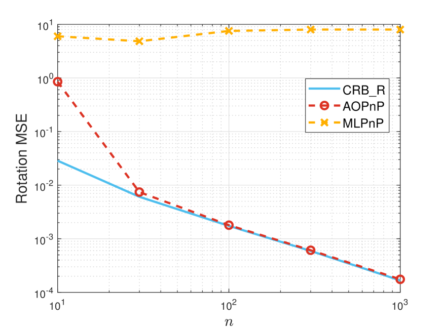
(a) $\sigma=50$ pixels ($\bf R$)

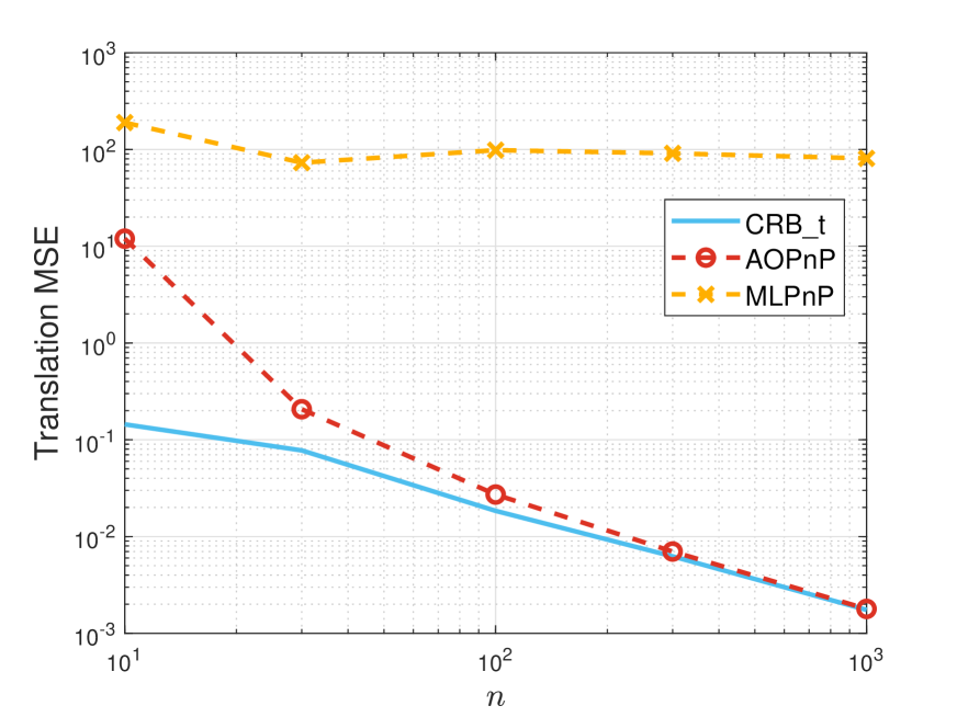
(b) $\sigma=50$ pixels ($\bf t$)

Figure 20: MSEs of PnP pose estimates.

Appendix E MSE of the MLPnP estimator when $\sigma=50$ pixels

Here, we set $\sigma=50$ pixels. The result is shown in Figure 20. In this case, the initial value of the MLPnP falls beyond the attraction neighborhood of the global minimum of (13). As a result, GN iterations drive the solution further away from the global minimizer, yielding a large MSE. Since the proposed AOPnP estimator is $\sqrt{n}$-consistent in its first step, a single GN iteration can make it asymptotically reach the CRB.

References

• [1] A. Z. Taddese, P. R. Slawinski, M. Pirotta, E. De Momi, K. L. Obstein, and P. Valdastri, “Enhanced real-time pose estimation for closed-loop robotic manipulation of magnetically actuated capsule endoscopes,” The International journal of robotics research, vol. 37, no. 8, pp. 890–911, 2018.
• [2] M. Zhang, X. Zuo, Y. Chen, Y. Liu, and M. Li, “Pose estimation for ground robots: On manifold representation, integration, reparameterization, and optimization,” IEEE Transactions on Robotics, vol. 37, no. 4, pp. 1081–1099, 2021.
• [3] S. Lilge, T. D. Barfoot, and J. Burgner-Kahrs, “Continuum robot state estimation using gaussian process regression on se (3),” The International Journal of Robotics Research, vol. 41, no. 13-14, pp. 1099–1120, 2022.
• [4] V. Lepetit, F. Moreno-Noguer, and P. Fua, “Epnp: An accurate o (n) solution to the pnp problem,” International Journal of Computer Vision, vol. 81, no. 2, pp. 155–166, 2009.
• [5] S. Urban, J. Leitloff, and S. Hinz, “Mlpnp-a real-time maximum likelihood solution to the perspective-n-point problem,” arXiv:1607.08112, 2016.
• [6] G. Terzakis and M. Lourakis, “A consistently fast and globally optimal solution to the perspective-n-point problem,” in Computer Vision–ECCV 2020: 16th European Conference, Glasgow, UK, August 23–28, 2020, Proceedings, Part I 16.   Springer, 2020, pp. 478–494.
• [7] C. Xu, L. Zhang, L. Cheng, and R. Koch, “Pose estimation from line correspondences: A complete analysis and a series of solutions,” IEEE Transactions on Pattern Analysis and Machine Intelligence, vol. 39, no. 6, pp. 1209–1222, 2016.
• [8] P. Wang, G. Xu, Y. Cheng, and Q. Yu, “Camera pose estimation from lines: a fast, robust and general method,” Machine Vision and Applications, vol. 30, pp. 603–614, 2019.
• [9] Y. Liu, G. Chen, and A. Knoll, “Globally optimal camera orientation estimation from line correspondences by bnb algorithm,” IEEE Robotics and Automation Letters, vol. 6, no. 1, pp. 215–222, 2020.
• [10] A. Vakhitov, J. Funke, and F. Moreno-Noguer, “Accurate and linear time pose estimation from points and lines,” in European Conference on Computer Vision.   Springer, 2016, pp. 583–599.
• [11] A. Vakhitov, L. Ferraz, A. Agudo, and F. Moreno-Noguer, “Uncertainty-aware camera pose estimation from points and lines,” in Proceedings of the IEEE/CVF Conference on Computer Vision and Pattern Recognition, 2021, pp. 4659–4668.
• [12] T. Haidegger, “Autonomy for surgical robots: Concepts and paradigms,” IEEE Transactions on Medical Robotics and Bionics, vol. 1, no. 2, pp. 65–76, 2019.
• [13] B. Mildenhall, P. P. Srinivasan, M. Tancik, J. T. Barron, R. Ramamoorthi, and R. Ng, “Nerf: Representing scenes as neural radiance fields for view synthesis,” Communications of the ACM, vol. 65, no. 1, pp. 99–106, 2021.
• [14] S. Lynen, B. Zeisl, D. Aiger, M. Bosse, J. Hesch, M. Pollefeys, R. Siegwart, and T. Sattler, “Large-scale, real-time visual–inertial localization revisited,” The International Journal of Robotics Research, vol. 39, no. 9, pp. 1061–1084, 2020.
• [15] D. DeMenthon and L. S. Davis, “Exact and approximate solutions of the perspective-three-point problem,” IEEE Transactions on Pattern Analysis and Machine Intelligence, vol. 14, no. 11, pp. 1100–1105, 1992.
• [16] L. Kneip, D. Scaramuzza, and R. Siegwart, “A novel parametrization of the perspective-three-point problem for a direct computation of absolute camera position and orientation,” in CVPR 2011.   IEEE, 2011, pp. 2969–2976.
• [17] M. Bujnak, Z. Kukelova, and T. Pajdla, “A general solution to the p4p problem for camera with unknown focal length,” in 2008 IEEE Conference on Computer Vision and Pattern Recognition.   IEEE, 2008, pp. 1–8.
• [18] B. Triggs, “Camera pose and calibration from 4 or 5 known 3d points,” in Proceedings of the Seventh IEEE International Conference on Computer Vision, vol. 1.   IEEE, 1999, pp. 278–284.
• [19] C.-P. Lu, G. D. Hager, and E. Mjolsness, “Fast and globally convergent pose estimation from video images,” IEEE transactions on pattern analysis and machine intelligence, vol. 22, no. 6, pp. 610–622, 2000.
• [20] G. Pavlakos, X. Zhou, A. Chan, K. G. Derpanis, and K. Daniilidis, “6-dof object pose from semantic keypoints,” in 2017 IEEE international conference on robotics and automation (ICRA).   IEEE, 2017, pp. 2011–2018.
• [21] R. Hartley and A. Zisserman, Multiple view geometry in computer vision.   Cambridge university press, 2003.
• [22] J. A. Hesch and S. I. Roumeliotis, “A direct least-squares (dls) method for pnp,” in Proceedings of IEEE International Conference on Computer Vision (ICCV), 2011, pp. 383–390.
• [23] Y. Zheng, Y. Kuang, S. Sugimoto, K. Astrom, and M. Okutomi, “Revisiting the pnp problem: A fast, general and optimal solution,” in Proceedings of the IEEE International Conference on Computer Vision, 2013, pp. 2344–2351.
• [24] L. Zhou and M. Kaess, “An efficient and accurate algorithm for the perspecitve-n-point problem,” in 2019 IEEE/RSJ International Conference on Intelligent Robots and Systems (IROS).   IEEE, 2019, pp. 6245–6252.
• [25] M. Dhome, M. Richetin, J.-T. Lapreste, and G. Rives, “Determination of the attitude of 3d objects from a single perspective view,” IEEE transactions on pattern analysis and machine intelligence, vol. 11, no. 12, pp. 1265–1278, 1989.
• [26] L. Zhou, D. Koppel, and M. Kaess, “A complete, accurate and efficient solution for the perspective-n-line problem,” IEEE Robotics and Automation Letters, vol. 6, no. 2, pp. 699–706, 2020.
• [27] Y. Liu, T. S. Huang, and O. D. Faugeras, “Determination of camera location from 2-d to 3-d line and point correspondences,” IEEE Transactions on pattern analysis and machine intelligence, vol. 12, no. 1, pp. 28–37, 1990.
• [28] S. Christy and R. Horaud, “Iterative pose computation from line correspondences,” Computer vision and image understanding, vol. 73, no. 1, pp. 137–144, 1999.
• [29] B. Přibyl, P. Zemčík, and M. Čadík, “Absolute pose estimation from line correspondences using direct linear transformation,” Computer Vision and Image Understanding, vol. 161, pp. 130–144, 2017.
• [30] F. M. Mirzaei and S. I. Roumeliotis, “Globally optimal pose estimation from line correspondences,” in 2011 IEEE International Conference on Robotics and Automation.   IEEE, 2011, pp. 5581–5588.
• [31] A. Ansar and K. Daniilidis, “Linear pose estimation from points or lines,” IEEE Transactions on Pattern Analysis and Machine Intelligence, vol. 25, no. 5, pp. 578–589, 2003.
• [32] L. Zhou, Y. Yang, M. Abello, and M. Kaess, “A robust and efficient algorithm for the pnl problem using algebraic distance to approximate the reprojection distance,” in Proceedings of the AAAI Conference on Artificial Intelligence, vol. 33, no. 01, 2019, pp. 9307–9315.
• [33] S. Ramalingam, S. Bouaziz, and P. Sturm, “Pose estimation using both points and lines for geo-localization,” in 2011 IEEE International Conference on Robotics and Automation.   IEEE, 2011, pp. 4716–4723.
• [34] L. Zhou, J. Ye, and M. Kaess, “A stable algebraic camera pose estimation for minimal configurations of 2d/3d point and line correspondences,” in Computer Vision–ACCV 2018: 14th Asian Conference on Computer Vision, Perth, Australia, December 2–6, 2018, Revised Selected Papers, Part IV 14.   Springer, 2019, pp. 273–288.
• [35] H. Li, J. Yao, X. Lu, and J. Wu, “Combining points and lines for camera pose estimation and optimization in monocular visual odometry,” in 2017 IEEE/RSJ International Conference on Intelligent Robots and Systems (IROS).   IEEE, 2017, pp. 1289–1296.
• [36] L. Sun and Z. Deng, “Certifiably optimal and robust camera pose estimation from points and lines,” IEEE Access, vol. 8, pp. 124 032–124 054, 2020.
• [37] S. Agostinho, J. Gomes, and A. Del Bue, “Cvxpnpl: A unified convex solution to the absolute pose estimation problem from point and line correspondences,” Journal of Mathematical Imaging and Vision, vol. 65, no. 3, pp. 492–512, 2023.
• [38] L. Ferraz Colomina, X. Binefa, and F. Moreno-Noguer, “Leveraging feature uncertainty in the pnp problem,” in Proceedings of the BMVC 2014 British Machine Vision Conference, 2014, pp. 1–13.
• [39] G. Zeng, S. Chen, B. Mu, G. Shi, and J. Wu, “Cpnp: Consistent pose estimator for perspective-n-point problem with bias elimination,” in 2023 IEEE International Conference on Robotics and Automation (ICRA).   IEEE, 2023, pp. 1940–1946.
• [40] A. Bartoli and P. Sturm, “The 3d line motion matrix and alignment of line reconstructions,” International Journal of Computer Vision, vol. 57, pp. 159–178, 2004.
• [41] T. Schops, J. L. Schonberger, S. Galliani, T. Sattler, K. Schindler, M. Pollefeys, and A. Geiger, “A multi-view stereo benchmark with high-resolution images and multi-camera videos,” in Proceedings of the IEEE conference on computer vision and pattern recognition, 2017, pp. 3260–3269.
• [42] T. Werner and A. Zisserman, “New techniques for automated architectural reconstruction from photographs,” in Proceedings of the European Conference on Computer Vision (ECCV).   Springer, 2002, pp. 541–555.
• [43] B. Mu, E.-W. Bai, W. X. Zheng, and Q. Zhu, “A globally consistent nonlinear least squares estimator for identification of nonlinear rational systems,” Automatica, vol. 77, pp. 322–335, 2017.
• [44] P. Stoica and T. Söderström, “Bias correction in least-squares identification,” International Journal of Control, vol. 35, no. 3, pp. 449–457, 1982.
• [45] G. Zeng, B. Mu, L. Shi, J. Chen, and J. Wu, “Consistent and asymptotically efficient localization from range-difference measurements,” IEEE Transactions on Information Theory, vol. 70, no. 4, pp. 3032–3045, 2024.
• [46] U. Helmke, K. Hüper, P. Y. Lee, and J. Moore, “Essential matrix estimation using gauss-newton iterations on a manifold,” International Journal of Computer Vision, vol. 74, pp. 117–136, 2007.
• [47] J. Zhao, “An efficient solution to non-minimal case essential matrix estimation,” IEEE Transactions on Pattern Analysis and Machine Intelligence, vol. 44, no. 4, pp. 1777–1792, 2020.
• [48] J. Nocedal and S. J. Wright, Numerical optimization.   Springer, 1999.
• [49] G. Zeng, B. Mu, J. Chen, Z. Shi, and J. Wu, “Global and asymptotically efficient localization from range measurements,” IEEE Transactions on Signal Processing, vol. 70, pp. 5041–5057, 2022.
• [50] M. Burri, J. Nikolic, P. Gohl, T. Schneider, J. Rehder, S. Omari, M. Achtelik, and R. Y. Siegwart, “The euroc micro aerial vehicle datasets,” The International Journal of Robotics Research, vol. 35, pp. 1157 – 1163, 2016. [Online]. Available: https://api.semanticscholar.org/CorpusID:9999787
• [51] K. M. Lynch and F. C. Park, Modern robotics.   Cambridge University Press, 2017.
• [52] P. Stoica and B. C. Ng, “On the cramér-rao bound under parametric constraints,” IEEE Signal Processing Letters, vol. 5, no. 7, pp. 177–179, 1998.
• [53] T. J. Moore, B. M. Sadler, and R. J. Kozick, “Maximum-likelihood estimation, the cramér–rao bound, and the method of scoring with parameter constraints,” IEEE Transactions on Signal Processing, vol. 56, no. 3, pp. 895–908, 2008.