Improving probabilistic forecasts of extreme wind speeds by training statistical post-processing models with weighted scoring rules

Abstract

Accurate forecasts of extreme wind speeds are of high importance for many applications. Such forecasts are usually generated by ensembles of numerical weather prediction (NWP) models, which however can be biased and have errors in dispersion, thus necessitating the application of statistical post-processing techniques. In this work we aim to improve statistical post-processing models for probabilistic predictions of extreme wind speeds. We do this by adjusting the training procedure used to fit ensemble model output statistics (EMOS) models – a commonly applied post-processing technique – and propose estimating parameters using the so-called threshold-weighted continuous ranked probability score (twCRPS), a proper scoring rule that places special emphasis on predictions over a threshold. We show that training using the twCRPS leads to improved extreme event performance of post-processing models for a variety of thresholds. We find a distribution body-tail trade-off where improved performance for probabilistic predictions of extreme events comes with worse performance for predictions of the distribution body. However, we introduce strategies to mitigate this trade-off based on weighted training and linear pooling. Finally, we consider some synthetic experiments to explain the training impact of the twCRPS and derive closed-form expressions of the twCRPS for a number of distributions, giving the first such collection in the literature. The results will enable researchers and practitioners alike to improve the performance of probabilistic forecasting models for extremes and other events of interest.

Keywords Probabilistic Weather Forecasting  $\cdot$ Statistical post-processing  $\cdot$ Scoring Rules  $\cdot$ Wind speed  $\cdot$ Extreme Events

1 Introduction

Extreme weather events such as heavy precipitation or windstorms have the potential to cause tremendous damage to lives and livelihoods. To mitigate their impact the development of early warning systems is crucial, which rely on accurate forecasts of relevant extremes. In this work we aim to improve statistical and machine learning models for probabilistic predictions of extreme wind speeds for applications to the post-processing of numerical weather prediction (NWP) wind speed forecasts.

Weather forecasts are usually generated by ensembles of NWP models, each with different initial conditions to quantify the uncertainty present in atmospheric phenomena. These ensembles, however, often contain biases and errors in dispersion, thus they necessitate the application of statistical post-processing techniques to generate accurate and well-calibrated probabilistic forecasts. This can be especially relevant for extreme events, whose forecasts might be improved most from post-processing, but which also require special care when using common techniques (Friederichs and Thorarinsdottir, 2012; Williams et al., 2014; Friederichs et al., 2018; Hess, 2020; Velthoen et al., 2023).

For post-processing of wind speed forecasts with particular focus on extremes, different models have been proposed in the literature. Lerch and Thorarinsdottir (2013) suggest post-processing based on ensemble model output statistics (EMOS, Gneiting et al., 2005) – a commonly applied post-processing technique – using the truncated normal and generalized extreme value (GEV) distributions as well as a regime switching model. Baran and Lerch (2015) propose post-processing based on the log-normal and truncated normal distributions as well as regime switching between the two. Allen et al. (2021a) incorporate weather regimes based on the North Atlantic Oscillation into their wind speed post-processing based on truncated logistic distributions, showing that this leads to improved predictive performance at extremes. Oesting et al. (2017) introduce post-processing of wind gusts forecasts based on a bivariate Brown-Resnick process.

Whilst the above authors propose different model structures that enable more accurate inference, we follow a different approach and change the training procedure used to fit models, in order to improve performance at extremes. This can in future work be readily extended to different model specifications. In order to improve the performance of predictive models at extremes, in recent times, a number of different authors have suggested to adjust loss functions used for the training of these models, which are often based on deep neural networks (Ding et al., 2019; Chen et al., 2022; Hess and Boers, 2022; Scheepens et al., 2023; Olivetti and Messori, 2024). However these works focus mostly on deterministic forecasts and as we show in section 3 the weighting schemes that these authors propose might not be suitable for probabilistic forecasts as they lead to "hedging" of the forecast distribution.

We propose adjusting training by estimating models using weighted proper scoring rules, in particular the so-called threshold-weighted continuous ranked probability score (twCRPS). This proper scoring rule, introduced by Gneiting and Ranjan (2011) has long been used for evaluation of predictive models, but to the authors’ knowledge not yet for systematic parameter optimization. In this work we focus on post-processing using Ensemble Model Output Statistics (EMOS), a typical post-processing method, and introduce the usage of the twCRPS to estimate the model parameters. We show that this improves predictive performance for extremes, for a variety of extremal thresholds. We set out some of the choices and challenges that forecasters need to consider when doing this, and describe the effects of these choices in real and simulated data, closing with recommendations of what to consider when applying this in operational settings. We also give different characterizations of the twCRPS and derive closed-form expressions for a number of predictive distributions.

This article is organized as follows. First, in section 2 we will present the data and methods used for post-processing in this study. We will then consider a motivating example in section 3 to highlight the need for propriety of scores used for the training of probabilistic forecasting models for extremes. In section 4 we introduce weighted scoring rules and the threshold-weighted continuous ranked probability score (twCRPS) that we use in section 5.1 to train post-processing models with a focus on extreme wind speeds. We show that this improves forecast performance for extremes and discuss some choices and challenges that forecasters might encounter in sections 5.1, 5.2 and 5.3, namely the body-tail trade-off, the role of the threshold for training models as well as sample based estimation. In section 6 we propose two strategies to balance different objectives that forecasters might encounter when wanting to improve forecasts for extremes: how to balance the forecast performance for the distribution body and the distribution tails. Finally, in section 7 we present a number of synthetic experiments to better understand the training impact of the twCRPS and interpret our results. We conclude in section 8, discussing the results and giving some recommendations for forecasters wishing to apply the methodology. In the appendix we give a number of different characterizations of the twCRPS and derive closed-form expressions for a number of distributions.

2 Data and methods

In this section we briefly describe the data and methods used for post-processing of wind speed forecasts.

2.1 Data

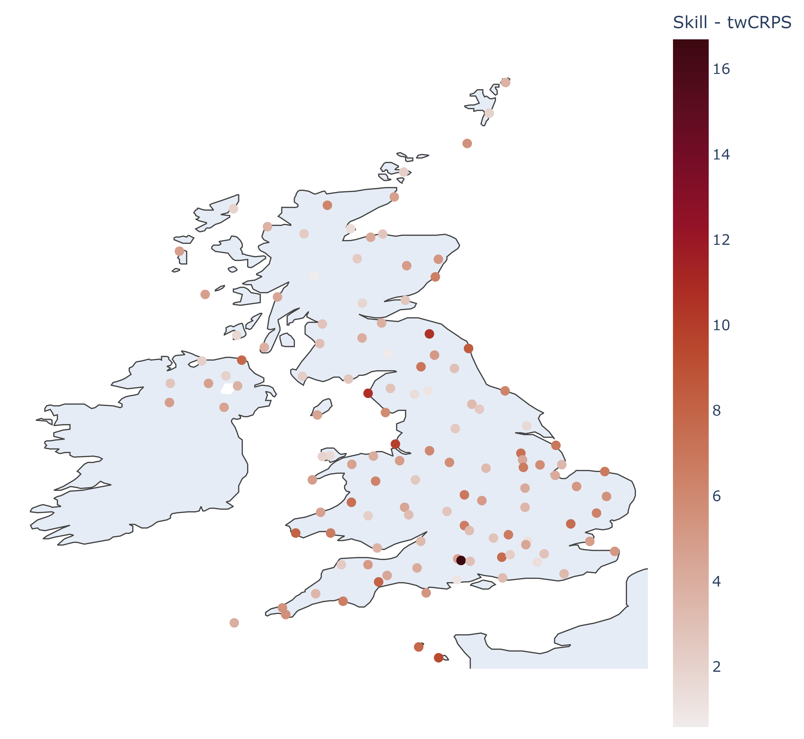
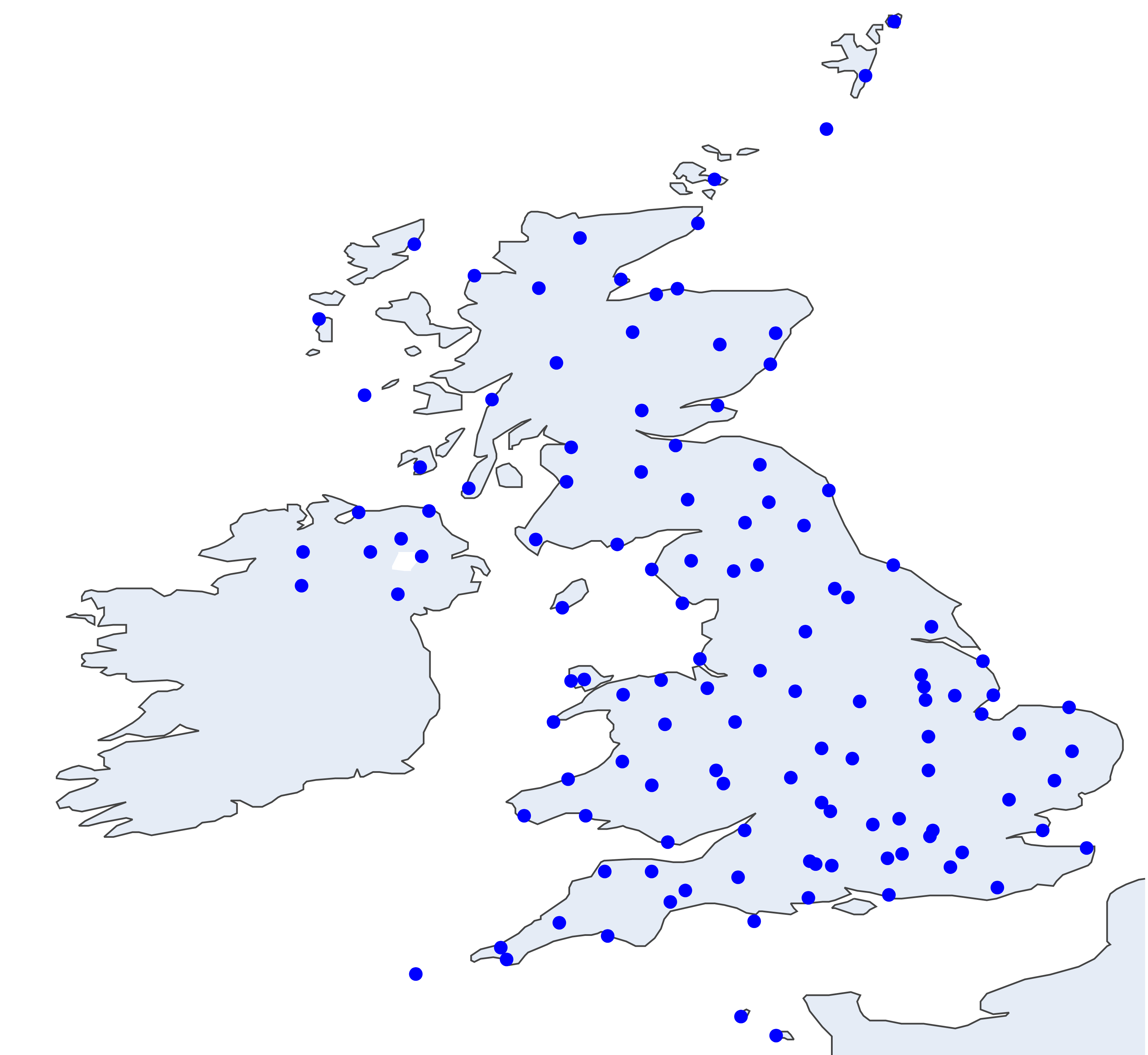
In this study we consider forecasts of 10m wind speed at surface observation stations in the United Kingdom at a lead time of 48h, initialized between 1 April 2019 and 31 March 2022. The forecasts are taken from the 0000 UTC initialization of the Met Office global ensemble prediction system (MOGREPS-G, Walters et al. 2017; Porson et al. 2020), an 18-member ensemble (including the unperturbed control run) with a horizontal resolution of 20km. The forecasts are bilinearly regridded to the locations of 124 surface synoptic observation (SYNOP) stations in the United Kingdom (see Figure 1 for the locations) and verified against wind speed observations (10min average of 10m wind speed) there. We assume the forecast ensemble to be exchangeable and summarize it by the ensemble mean and ensemble standard deviation. We use forecasts issued between 1 April 2019 and 31 December 2020 for training and forecasts issued between 1 January 2021 and 31 March 2022 as an independent test set.

Figure 1: Locations of 124 SYNOP stations used for the verification of wind speed forecasts.

2.2 Methods

In this study we consider post-processing based on ensemble model output statistics (EMOS) also known as non-homogeneous (Gaussian) regression (NGR, Jewson et al. 2004; Gneiting et al. 2005). EMOS is one of the most commonly used post-processing methods, both in research works and operational forecasting environments (Hess, 2020; Roberts et al., 2023), owing to its simplicity, robustness and extensibility. Within the EMOS framework the variable of interest (wind speed $W$ here) is assumed to follow a parametric distribution $\mathcal{D}$ whose parameters are modelled in terms of the raw ensemble $x_{1},\dots,x_{N}$, often summarized by ensemble mean $m$ and ensemble standard deviation $s$. In this study, we consider both truncated normal $\mathcal{D}=\mathcal{N}_{0}$ (Thorarinsdottir and Gneiting, 2010) and truncated logistic $\mathcal{D}=\mathcal{L}_{0}$ (Messner et al., 2014; Scheuerer and Möller, 2015) as predictive distributions for wind speed (both truncated at zero). In addition to the ensemble mean and ensemble standard deviation we also include sine-cosine transformations of the normalized day of year ($\text{ndoy}:=2\pi\tfrac{\text{day of year}}{365.25}$) as predictors, to account for seasonality (Lang et al., 2020). We model:

$$W\,|\,m,s\sim\mathcal{D}(\mu,\sigma),$$ (1)

$$\mu=\alpha+\beta m+\lambda_{\mu,{\rm sin}}\sin\left(\text{ndoy}\right)+\lambda_{\mu,{\rm cos}}\cos\left(\text{ndoy}\right),$$ (2)

$$\log\sigma=\gamma+\delta s+\lambda_{\sigma,{\rm sin}}\sin\left(\text{ndoy}\right)+\lambda_{\sigma,{\rm cos}}\cos\left(\text{ndoy}\right).$$ (3)

Here $\mu$ and $\sigma$ are the location and scale parameters of the predictive distribution $\mathcal{D}$.
EMOS models are usually fit by either minimizing the negative log-likelihood or the continuous ranked probability score (CRPS). For a probabilistic forecast given through a cumulative distribution function (CDF) $F$ and an observation $y$ the latter is defined as:

$$\text{CRPS}(F,y)=\int_{-\infty}^{\infty}\left[F(z)-\mathbb{1}\{z\geq y\}\right]^{2}dz.$$ (4)

Both the CRPS and the negative log-likelihood are proper scoring rules (Gneiting and Raftery, 2007), meaning that in expectation they are minimal when the forecast distribution is the "true" distribution (see section 4 for some more discussion of propriety). Closed-form expressions of the CRPS exist for the truncated normal and truncated logistic distributions (see Jordan et al., 2019) and are used for the minimization. In this study EMOS models are fit separately for each site.

Unless otherwise stated in this paper we use a Broyden-Fletcher-Goldfarb-Shanno (BFGS) quasi-Newton optimizer (Nocedal and Wright, 2006) with empirical gradient estimates for optimizing scoring functions, which falls back onto a Nelder-Mead optimizer (Nelder and Mead, 1965) should it fail. We follow the practice of the crch package (Messner et al., 2022) and use the coefficients of a linear regression as starting values for the location parameters ($\alpha,\beta,\lambda_{\mu,{\rm sin}},\lambda_{\mu,{\rm cos}}$) and the exponentially transformed standard error as the starting value of the intercept of the scale parameter ($\gamma$), whilst setting all other scale parameters ($\delta,\lambda_{\sigma,{\rm sin}},\lambda_{\sigma,{\rm cos}}$) initially to zero.

3 Motivating the use of proper scoring rules

In order to improve the performance of data-driven models for prediction of extreme events multiple authors propose adjusting loss functions used to learn parameters of these models (e.g. Ding et al., 2019; Chen et al., 2022; Olivetti and Messori, 2024). Among others Hess and Boers (2022) and Scheepens et al. (2023) propose weighting schemes for loss functions to weight misprediction at extremes stronger during training. Many of the above authors focus on deterministic predictions of extremes, however as Friederichs and Thorarinsdottir (2012) point out to allow for the assessment of the potentially large uncertainty in predictions of extreme events, such predictions should be "probabilistic in nature". In this section we will study the effect of a loss function weighting strategy for probabilistic extreme event forecasting in the setting of post-processing. This is to motivate the need for proper scoring rules when training probabilistic forecasting models.

Hess and Boers (2022) propose a weighting scheme for loss functions to penalize strongly the mis-prediction of high precipitation values during training. They only consider deterministic forecasts, trained using root mean squared error (RMSE), however we consider this weighting scheme adapted for the training of probabilistic post-processing models for wind speed. We consider EMOS post-processing models using a truncated normal distribution, trained by minimizing the following loss (henceforth referred to as HB-loss):

$$L(F,y):=w_{a,b}(y)\ \text{CRPS}(F,y)\ \ \ \ \text{ with }\ \ \ \ w_{a,b}(y):=\min\left[1,\exp\left(\tfrac{y-a}{b}\right)\right].$$ (5)

This weighting scheme means that prediction quality (measured through the CRPS) of high observed wind speed values will carry more weight during training. We choose $a$ as the location-wise 80th percentile of the observations of the training dataset and $b$ as the location-wise standard deviation of the observational training dataset. We score predictions against EMOS models trained classically using the CRPS.

Investigating the trained model’s performance on the test set we find that when training EMOS post-processing models using the HB-loss the resulting models have much lower HB-loss on the test set (16% lower) compared to the CRPS-trained model. Looking at the dataset of test set extremes – wind speed values over the location-wise 80th percentile of the training set $\tau$ – we find that the HB-trained model is far better than the CRPS-trained model having 26% better RMSE and 6% better CRPS respectively on this dataset. The model has good out-of-sample HB-loss performance and seems to be able to capture the intensity of extremes quite well.

Next to the intensity we also analyse the performance of the models at predicting the occurrence of extremes by evaluating the Brier Score – a proper scoring rule for binary events/threshold exceedances:

$$BS_{\tau}(F,y):=\left[F(\tau)-\mathbb{1}\{y\geq\tau\}\right]^{2}.$$ (6)

We find that the HB-trained model strongly overpredicts extremes, having 12% worse Brier Score than the CRPS-trained model. A similar picture can be seen by considering probability integral transform (PIT) histograms (Thorarinsdottir and Schuhen, 2018). These are histograms of the predictive CDF evaluated at the observation and should appear uniform under calibration. Figure 2 shows the histograms for the CRPS and HB-trained model. Whilst the CRPS-trained model seems approximately calibrated the HB-trained model has a right tail that is much too heavy and seems to strongly underpredict values in the body of the climatological distribution.

Figure 2: PIT histograms for wind speed post-processing models using truncated normal distributions, trained using CRPS loss (left) and HB-loss (eq. 5, right).

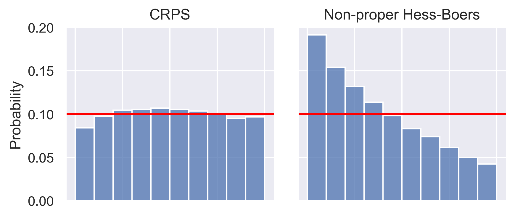
When evaluating only on test set extremes the HB model seems to be a suitable prediction model, however when considering the full dataset the model strongly overpredicts the occurrence of extremes and seems strongly mis-calibrated. A similar result also occurs with a very related strategy of oversampling extremes prior to training, often used to adjust for class imbalance in classification problems (van den Goorbergh et al., 2022). The need to evaluate not only the intensity of extreme event forecasts, but to do this jointly with the predicted occurrence has been highlighted by many authors and is commonly referred to as the "forecaster’s dilemma" (Lerch et al., 2017). If only forecasts of intensity are evaluated, then this encourages forecasters to overpredict extreme values, something that is not a problem in cases where there is no penalty for false-positive extreme event warnings. However in real applications this will quickly erode trust in any forecasting system and lead to economic costs. The CRPS is a proper scoring rule, thus using it for training and evaluation encourages honesty of the forecasters and calibrated forecasts. However when weighting the CRPS by an observed outcome, for example by restricting evaluation to the dataset of test set extremes or by using a weighting such as the HB-weighting, propriety is lost. This makes the score unsuitable for objective evaluation and for training (see next section).

4 Weighted scoring rules for assessing forecasts of extremes

The goal of probabilistic forecasting has been put by Gneiting et al. (2005) as to "maximize sharpness subject to calibration". Sharpness is a measure of the forecast distribution only and refers to the concentration of the forecast density function, whilst calibration is a joint property between observations and forecast and corresponds to the consistency between the forecast distributions and the observations. Proper scoring rules (Gneiting and Raftery, 2007) have been introduced for the evaluation (and training) of probabilistic forecasts. They assess both calibration and sharpness. Briefly, a scoring rule $S$ is proper when the following holds for any probabilistic forecast $F$ and "true" distribution $G$:

$$\mathbb{E}_{y\sim G}S(F,y)\geq\mathbb{E}_{y\sim G}S(G,y).$$ (7)

Here $S(F,y)$ is the score of the predictive CDF at the observation $y$ and $\mathbb{E}_{y\sim G}S(F,y)$ denotes its expectation over the distribution of $G$. A scoring rule is thus called proper when in expectation it is minimal at the true distribution. It is called strictly proper if equality in eq. 7 holds only when $F=G$.

When wanting to focus probabilistic forecast evaluation on certain events of interest such as extreme events over a threshold, one can try to restrict the evaluation to these events or weight them stronger. Mathematically, both correspond to constructing a scoring rule weighted by an observation: $\tilde{S}(F,y):=w(y)\ S(F,y)$. However, as Gneiting and Ranjan (2011) and Lerch et al. (2017) show, if the weighting function is non-constant the resulting scoring rule becomes non-proper. Concretely, the expected weighted score $\mathbb{E}_{y\sim G}\tilde{S}(F,y)$ is no longer minimal at $F=G$ but at the predictive distribution corresponding to the density

$$f(y)=\frac{w(y)g(y)}{\int w(z)g(z)dz}\propto w(y)g(y),$$ (8)

where $g$ is the density corresponding to $G$. Thus when evaluating probabilistic forecasting models using scoring rules restricted to an outcome (such as events over a threshold) or scoring rules weighted by some weighting function (such as the HB-loss) this encourages hedging of the forecast distribution, meaning a forecaster is encouraged to deviate from the true distribution in their prediction by an amount determined by the weighting function. This also affects model training as can be seen in section 3.

To address this problem Gneiting and Ranjan (2011) introduce proper weighted scores and especially the weighted continuous ranked probability score (wCRPS). These remain proper whilst focusing inference onto certain values of interest. The weighted CRPS is defined as

$$\text{wCRPS}(F,y)=\int_{-\infty}^{\infty}w(z)\left[F(z)-\mathbb{1}\{z\geq y\}\right]^{2}dz,$$ (9)

for a nonnegative weighting function $w$. This reduces to the unweighted CRPS (eq. 4) when $w(z)\equiv 1$. The canonical weighting is indicator weighting: $w_{\tau}(z)=\mathbb{1}\{z\geq\tau\}$, when there is interest in values above (or below) a certain threshold $\tau$, which then leads to the so-called threshold-weighted CRPS (twCRPS):

$$\text{twCRPS}_{\tau}(F,y)=\int_{\tau}^{\infty}\left[F(z)-\mathbb{1}\{z\geq y\}\right]^{2}dz.$$ (10)

The weighted CRPS and especially the threshold-weighted versions have become frequently used tools for forecast evaluation of extreme events (e.g. Lerch and Thorarinsdottir, 2013; Baran and Lerch, 2015; Baran and Nemoda, 2016; Allen et al., 2021b). They have also been generalized to multivariate versions (Allen et al., 2023b, a). In the following we will focus on the twCRPS as given in equation 10.

The CRPS corresponds to the integral over the Brier Score over all possible thresholds, whilst the twCRPS with threshold $\tau$ restricts the evaluation of this integral only to thresholds of interest, over $\tau$. Evaluation of a predictive CDF $F$ using the twCRPS with threshold $\tau$ corresponds to evaluating the censored CDF $\tilde{F}_{\tau}$, censored at $\tau$ using the classical CRPS, formally:

Lemma 4.1.

The threshold-weighted CRPS at threshold $\tau$ of the distribution $F$ is equal to the CRPS of the censored distribution $\tilde{F}_{\tau}$ with censored observation $\tilde{y}$:

$$\text{twCRPS}_{\tau}(F,y)=\text{CRPS}(\tilde{F}_{\tau},\tilde{y})$$ (11)

where $\tilde{y}:=v_{\tau}(y)=\max(y,\tau)$ and $\tilde{F}_{\tau}$ is the CDF censored at $\tau$:

$$\tilde{F}_{\tau}(x)=\begin{cases}0&\text{ if }x<\tau\\ F(x)&\text{ if }x\geq\tau\end{cases}.$$ (12)

This is alluded to already in Allen et al. (2023a). The proof is given in the appendix. Thus intuitively when using the twCRPS a forecaster effectively uses the full CRPS to evaluate the distribution $\tilde{F}_{\tau}$ that has all probability mass below the threshold collapsed onto the threshold itself, whilst remaining the same above the threshold. That way the exact form of the distribution below $\tau$ only influences the score via the probability mass for exceeding or falling below the threshold.

Closed-form expressions of the twCRPS exist for a number of distributions, for example Allen et al. (2021b) derive the twCRPS for the truncated logistic and Wessel et al. (2024) the twCRPS for the truncated normal distribution. To facilitate application of the twCRPS in future work the authors have collected from the literature and manually derived a number of closed-form twCRPS expressions for many often-used predictive distributions: the normal, logistic, Laplace, Student’s t, gamma, log-normal, log-logistic, generalized Pareto, exponential and uniform distributions as well as censored and truncated versions of these. These expressions, together with a number of different characterizations of the twCRPS, can be found in the Appendix.

The twCRPS also admits a formulation as an expectation (Taillardat et al., 2023; Allen et al., 2023a):

$$\text{twCRPS}_{\tau}(F,y)=\mathbb{E}_{X\sim F}|v_{\tau}(X)-v_{\tau}(y)|-\frac{1}{2}\mathbb{E}_{X,X^{\prime}\sim F}|v_{\tau}(X)-v_{\tau}(X^{\prime})|,$$ (13)

where $v_{\tau}$ is the so-called "chaining function":

$$v_{\tau}(x):=\begin{cases}x_{0}&\text{ if }x<\tau\\ x&\text{ if }x\geq\tau\end{cases}.$$ (14)

Here $x_{0}$ is an arbitrary point that all values below the threshold $\tau$ are mapped to. In the following we will use the canonical choice $x_{0}=\tau$ for which the chaining function is continuous. We will discuss the impact of other choices of $x_{0}$ on sample based optimization of the twCRPS in appendix D. The formulation of the twCRPS as an expectation can be used to approximate it via samples from a predictive distribution, i.e. using the estimator

$$\widehat{\text{twCRPS}_{\tau}}(F,y)=\frac{1}{N}\sum_{i=1}^{N}|v_{\tau}(X_{i})-v_{\tau}(y)|-\frac{1}{2N^{2}}\sum_{i,j=1}^{N}|v_{\tau}(X_{i})-v_{\tau}(X_{j})|,$$ (15)

where $X_{1},\dots,X_{N}\sim F$ are samples from the predictive CDF. This can be useful for example in cases where no closed-form expression is available.

Although the twCRPS has been frequently used for evaluation of probabilistic forecasting models for extremes, it has – to the authors’ best knowledge – to this date not been used for training post-processing models i.e. as a loss function for parameter estimation. However, given that weighted and threshold-weighted scores are proper – something that section 3 showed is important also for model training – and the relevance of reliable forecasts for extremes, we will study their usage for the training of EMOS post-processing models for wind speed, for both truncated normal and truncated logistic EMOS models.

5 Results: training with weighted scoring rules

We study the usage of the weighted CRPS for the training of post-processing models, to improve probabilistic predictions of extreme wind speeds. The weighted CRPS is a proper scoring rule, thus using it for evaluation and training will favour calibrated-sharp forecasts. We focus on the canonical threshold weighting due to the availability of closed-form solutions, which helps with the optimization. We consider training EMOS models using the following proper scores:

• CRPS,

• Negative log likelihood,

• twCRPS with a threshold $\tau$.

Here the CRPS and log-likelihood models serve as baselines, whilst the twCRPS puts special emphasis on values above a threshold $\tau$. For optimizing the score functions we use the closed-form expressions for the CRPS and twCRPS for the truncated normal and truncated logistic distributions (see appendix B).

5.1 Effect of weighted training

We consider thresholds $\tau$ defined as the location-wise 80th and 90th percentile of the training dataset and train using the scores in section 5. In practical applications most likely absolute thresholds defined by user needs will be of relevance, however to show the general applicability of the method we use percentile based thresholds here as in Sharpe et al. (2018); Sharpe and Stewart (2019); Sharpe (2022). Figure 12 in the appendix shows the 80th and 90th percentile threshold at each station. We report skill scores relative to the model trained using CRPS ("CRPS-trained model")

(a) Evaluated using twCRPSS

(b) Evaluated using CRPSS

Figure 3: Threshold-weighted CRPS skill score (left, a) and CRPS skill score (right, b), both relative to the CRPS-trained model, for wind speed EMOS using truncated normal and truncated logistic distributions. Models are trained using log likelihood, and twCRPS. Thresholds for training and evaluation of the twCRPS are defined as locationwise 80th and 90th percentile of the training dataset.

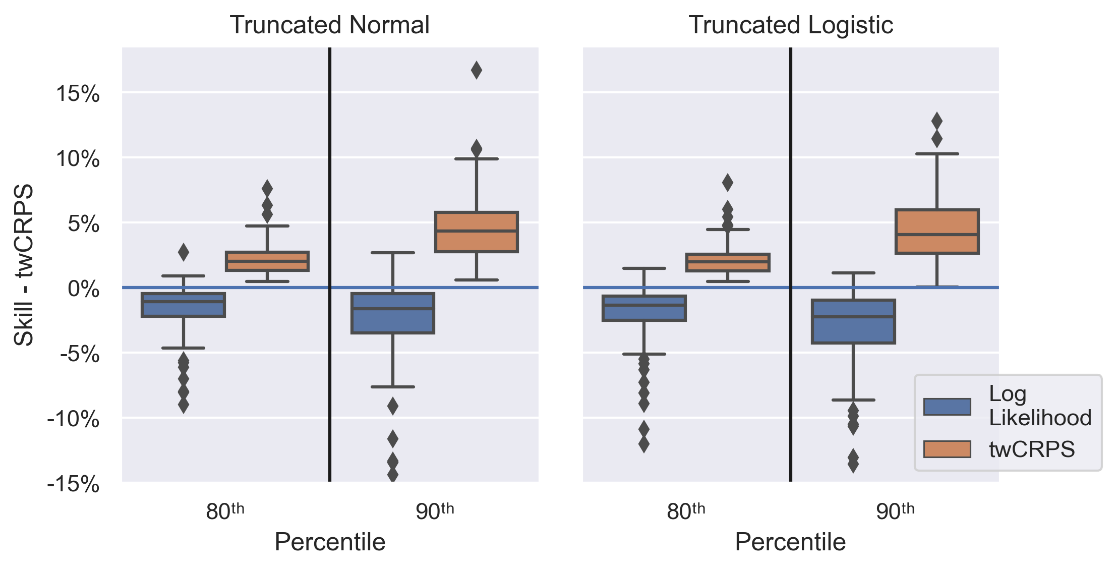
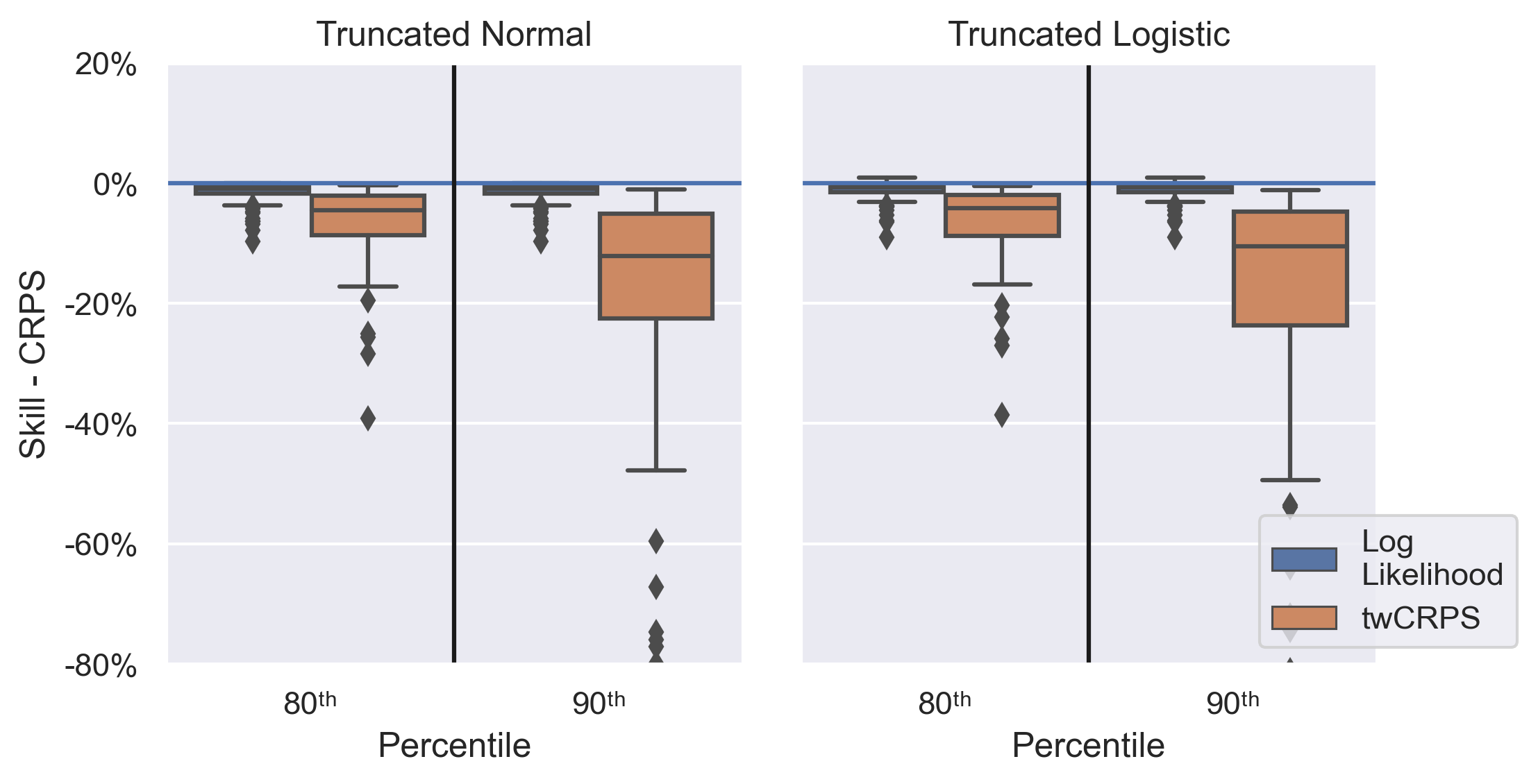
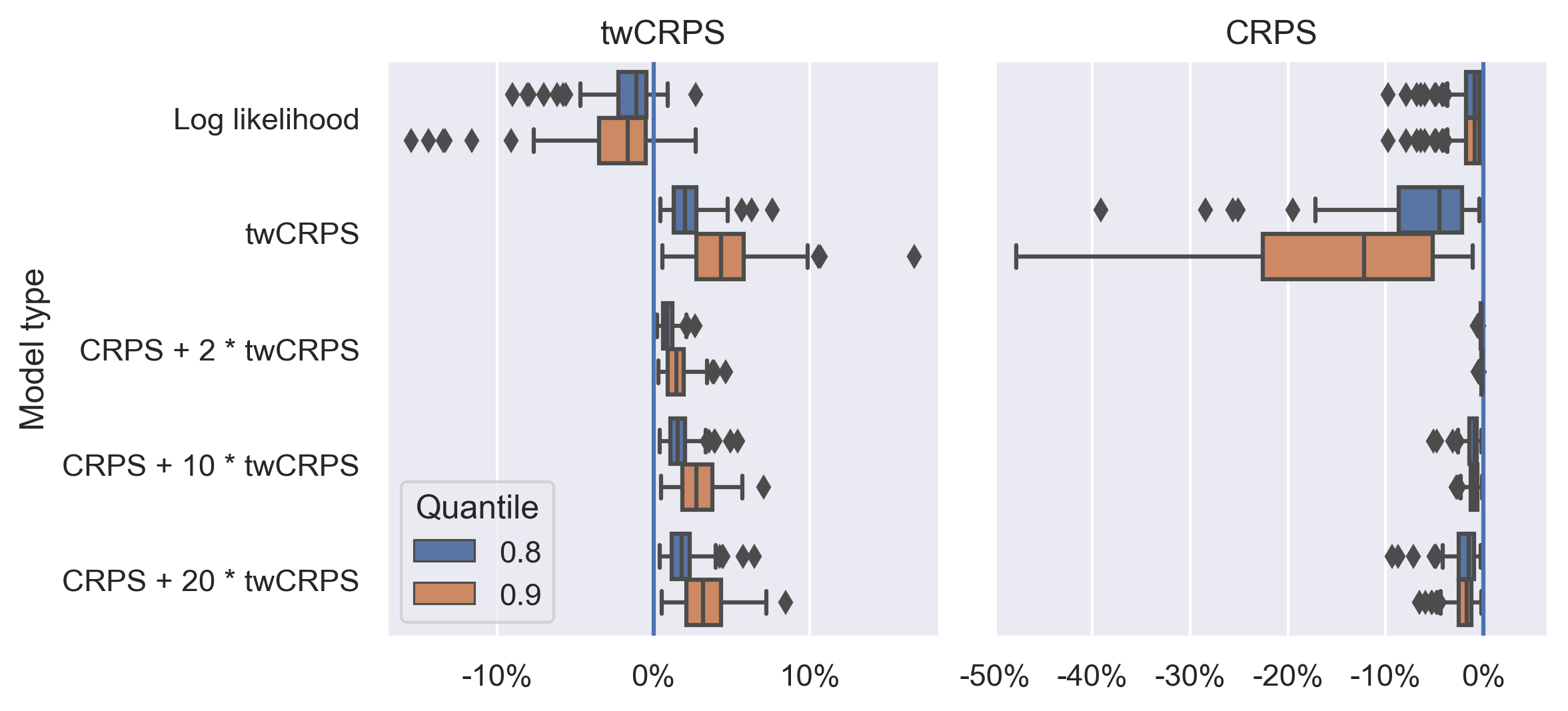
Figure 3(a) shows for all models the threshold-weighted CRPS skill score over the CRPS-trained model evaluated on the test set, for the 80th and 90th locationwise percentile thresholds (used for both training and evaluation) for both truncated normal and truncated logistic predictive distributions. Training using a twCRPS leads to improved predictions of extremes, as measured by the twCRPS on the test set. These improvements average around $\sim 2.5$% for the 80th and around 5% for the 90th percentile threshold and up to $\sim 8$% and $\sim 15$% respectively. The twCRPS improvements also show in terms of Brier skill score where we see that by training using a twCRPS one also gets better predictions of the occurrence of threshold exceedances of around 1.7% for the 80th and around 0.9% for the 90th percentile threshold in the truncated normal and around 1.6% and 0.7% in the truncated logistic case (see table 1 in the appendix for the Brier skill score for both distributions for a variety of evaluation thresholds). Finally the improvements seem to be distributed heterogeneously over space, possibly with slightly stronger improvements for stations closer to the coast (Figure 13 in the appendix). The log-likelihood training performs worse in terms of CRPS and twCRPS than the CRPS-trained model which is in line with previous studies (Gneiting et al., 2005; Gebetsberger et al., 2018).

The twCRPS improvement seems however to be linked to a loss in CRPS as can be seen in Figure 3(b) which shows the CRPS skill over the CRPS-trained model, evaluated on the test set. The twCRPS-trained model loses CRPS skill, compared to the CRPS-trained model for both the 80th and even stronger for the 90th percentile threshold. The latter threshold improves more in terms of twCRPS, but also loses more in terms of CRPS, irrespective of the predictive distribution.

There seems to be a trade-off between CRPS and twCRPS performance, which we investigate more closely. We focus on the truncated normal distribution, the 80th percentile and twCRPS training. Figure 4(a) shows the twCRPS skill improvement against the CRPS skill loss for all locations. We see a trade-off between the two objectives for this model, which have different ranges of skill change, meaning that a twCRPS improvement might lead to a much stronger CRPS loss. Figure 4(b) shows that the CRPS loss and twCRPS improvement relate to the distance between the EMOS parameters of the CRPS-trained and twCRPS-trained model. The figure shows the Euclidean norm of the difference between the EMOS parameters of the twCRPS-trained and CRPS-trained model, plotted against CRPS skill loss (blue) and twCRPS skill improvement (orange), both relative to the CRPS-trained model. The bigger the difference in EMOS parameters, the bigger the twCRPS improvement can be, however this comes with a larger CRPS skill loss as well.

(a) CRPS skill loss against twCRPS skill gain

(b) Parameter difference against twCRPS/CRPS change

Figure 4: CRPS-twCRPS trade-off for the truncated normal, twCRPS-trained model for the 80th percentile. Left (a): CRPS skill loss against twCRPS skill gain for all locations, both relative to the CRPS-trained model. Right (b) Difference in EMOS parameters between the twCRPS-trained model and the CRPS-trained model plotted against CRPS (blue) or twCRPS (orange) skill over the CRPS-trained model

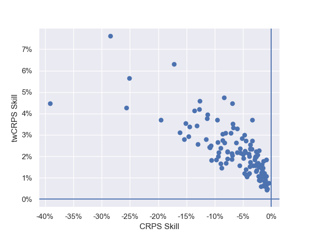
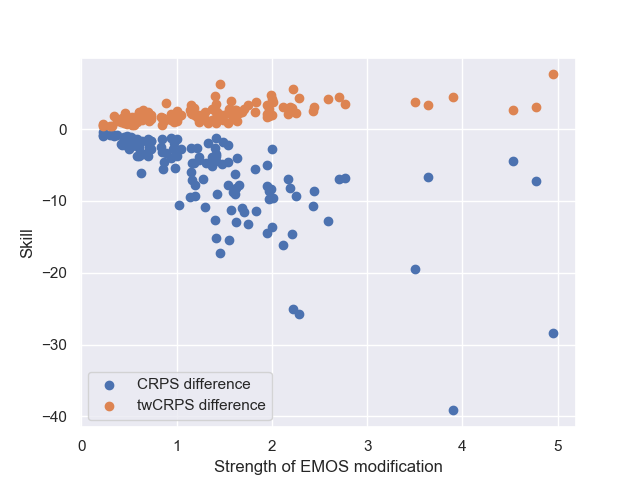
In summary, by optimizing the twCRPS one can improve extreme event performance of forecasts, as measured by twCRPS and Brier Score. This however comes at some cost in terms of CRPS – measuring the forecast performance for the whole distribution and the distribution body. The trade-off between CRPS and twCRPS performance can be seen as a classic distribution "body-tail trade-off" where an improved modelling of a distribution’s tails might come at the cost of capturing of the distribution’s body and vice-versa. This seems to hold for training thresholds defined as 80th and 90th percentile of the distribution, however in the next section we will study the effect of varying the training threshold.

5.2 Effect of the training threshold

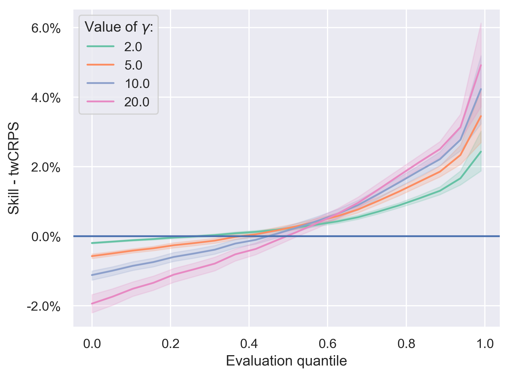
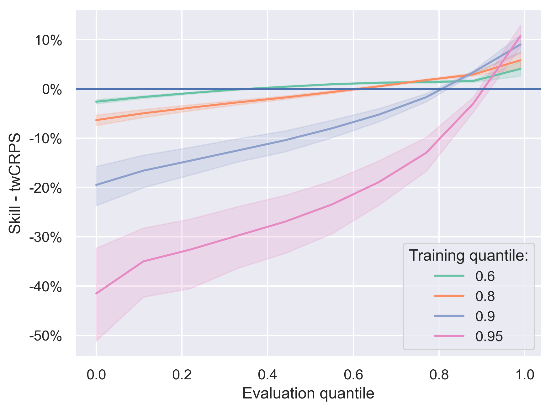
We study the effect of varying the threshold for training using the twCRPS and analyze this for the truncated normal case. Results for the truncated logistic distribution are similar. We train post-processing models using the twCRPS with thresholds as 60th, 80th, 90th and 95th percentile and evaluate against a range of different thresholds between the 0th (corresponding to the unweighted CRPS) to 99th percentile of the locationwise training dataset. Figure 5 shows the twCRPS skill (relative to the CRPS-trained model) as a function of the threshold for all four trained models. The model trained for a certain threshold seems to perform best at this threshold (and slightly lower) and has generally positive skill score for evaluation thresholds higher than the one it was trained for. However training with a twCRPS for a high quantile threshold leads to skill loss at lower quantiles and it seems the higher the training threshold / quantile the worse the twCRPS skill loss for lower evaluation thresholds / quantiles also becomes, manifesting in increasing slope of the skill curves. This means that model performance can be improved for many thresholds by training with a twCRPS, but should the distribution body performance be important it might be sensible to use lower thresholds. In these cases however the skill improvements for high quantiles also do not seem to be as substantial. Similar curves are also obtained when evaluating the Brier score (see figure 14 in the appendix).

Figure 5: twCRPS skill score (over the CRPS-trained model) as a function of the evaluation threshold for twCRPS-trained models trained using different thresholds. The bands represent 95% intervals over stations. The twCRPS for an evaluation quantile of $0.0$ corresponds to the unweighted CRPS.

5.3 Effect of sample-based estimation

In the sections above we have investigated the impact of training post-processing models using a twCRPS, optimizing closed-form solutions for the twCRPS for both truncated normal and truncated logistic distributions. However closed-form solutions like these might not be available in all cases, for example when a model does not follow a known distributional structure. In these cases the predictive distribution function might still be available via samples and one can estimate the twCRPS by approximating its representation as an expectation (equation 13). In the following we study whether sample based optimization of the twCRPS can also be effective for training models. We study again EMOS using the truncated normal distribution, trained using the twCRPS with a location-wise 80th and 90th percentile threshold. However we only compute the twCRPS by sampling from the model.

We find that sample-based optimization proves difficult. First the optimization algorithm has a strong influence. The BFGS algorithm frequently fails to find optimal parameters, even when using 1000 samples for each predictive distribution, which is most likely due to noisy empirical gradients and a noisy and relatively flat cost function. The Nelder-Mead optimizer, which is not based on gradients, can converge in some cases and for some starting values, after adjusting the tolerance to account for fluctuations in the twCRPS values. Similarly Adam (Kingma and Ba, 2017), a stochastic gradient descent algorithm, together with the reparametrization trick (Kingma and Welling 2022, see appendix C) to allow gradients with respect to the parameters, can converge with the right starting values. However, it is much slower than Nelder-Mead or BFGS-based optimization of the closed-form solutions. It also leads to EMOS models which are much less efficient i.e. have far smaller twCRPS improvement than training using the closed-form expression, if they have any improvement at all.

The sample-based twCRPS seems to represent a rather noisy and possibly very flat loss objective, whose optimization seems dominated by sampling uncertainty. In certain cases (e.g. with starting values that are close to the solution and using exact gradients) the optimization can converge, however it is quite unstable. The results speak for using closed-form expressions for the optimization in cases in which these are available (see appendix B for a list of closed-form expressions) as the optimization objective seems much simpler to solve. However closed-form expressions might not be available in all cases, e.g. for very complex models, other weighting functions different from threshold weighting or when wanting to use multivariate weighted scores (Allen et al., 2023b, a). We defer the question of how to stabilize sample-based twCRPS optimization in these cases for future work. Also, the interested reader can find more analysis on sample based optimization in appendix D.

6 Forecast combinations

In section 5.1 we found a trade-off between twCRPS improvement and CRPS loss, when training using the twCRPS. A forecast distribution, it seems, can be very good for extremes but sub-optimal for values in the body of the climatological distribution. This can pose challenges for application. In the following we study two ways of combining the CRPS and twCRPS objectives to enable forecasters to balance the trade-off and adjust CRPS and twCRPS performance to their preferences. First we consider training EMOS models using weighted score combinations:

$$\text{CRPS}(F,y)+\gamma\cdot\text{twCRPS}_{\tau}(F,y).$$ (16)

These combine training using a CRPS and twCRPS and correspond to a weighted CRPS with weighting function $w(z)=1+\gamma\cdot\mathbb{1}(z\geq\tau)$, originally proposed by Thorarinsdottir and Schuhen (2018) for the assessment of forecasts. Other, non-threshold-based, weighting functions might also be usable to balance body-tail forecast performance, however indicator weighting has the advantage of closed-form solutions being available. In a second step we consider linear pooling between the CRPS-trained and twCRPS-trained model, to control twCRPS improvement and CRPS loss. We focus on the 80th percentile threshold for both truncated normal and truncated logistic distributions.

6.1 Weighted combinations

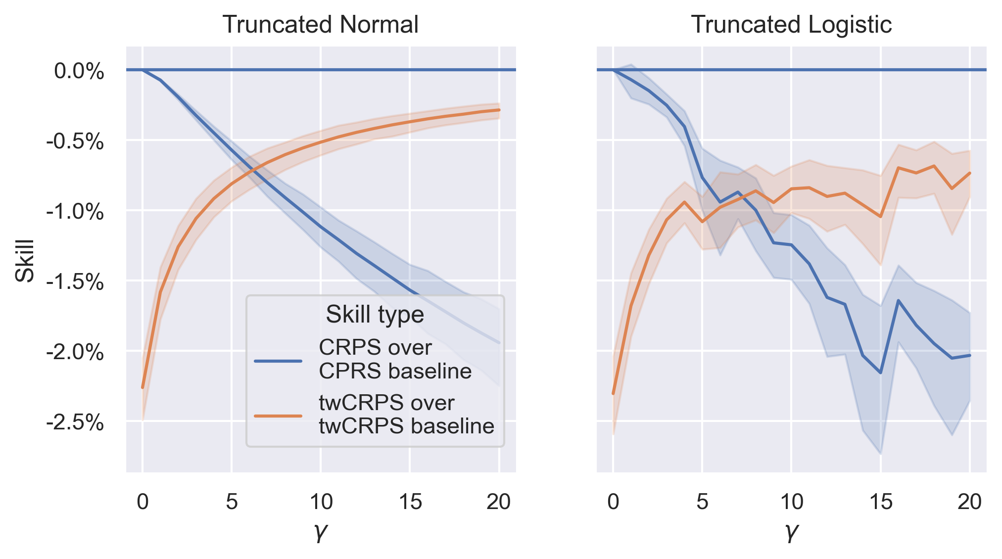
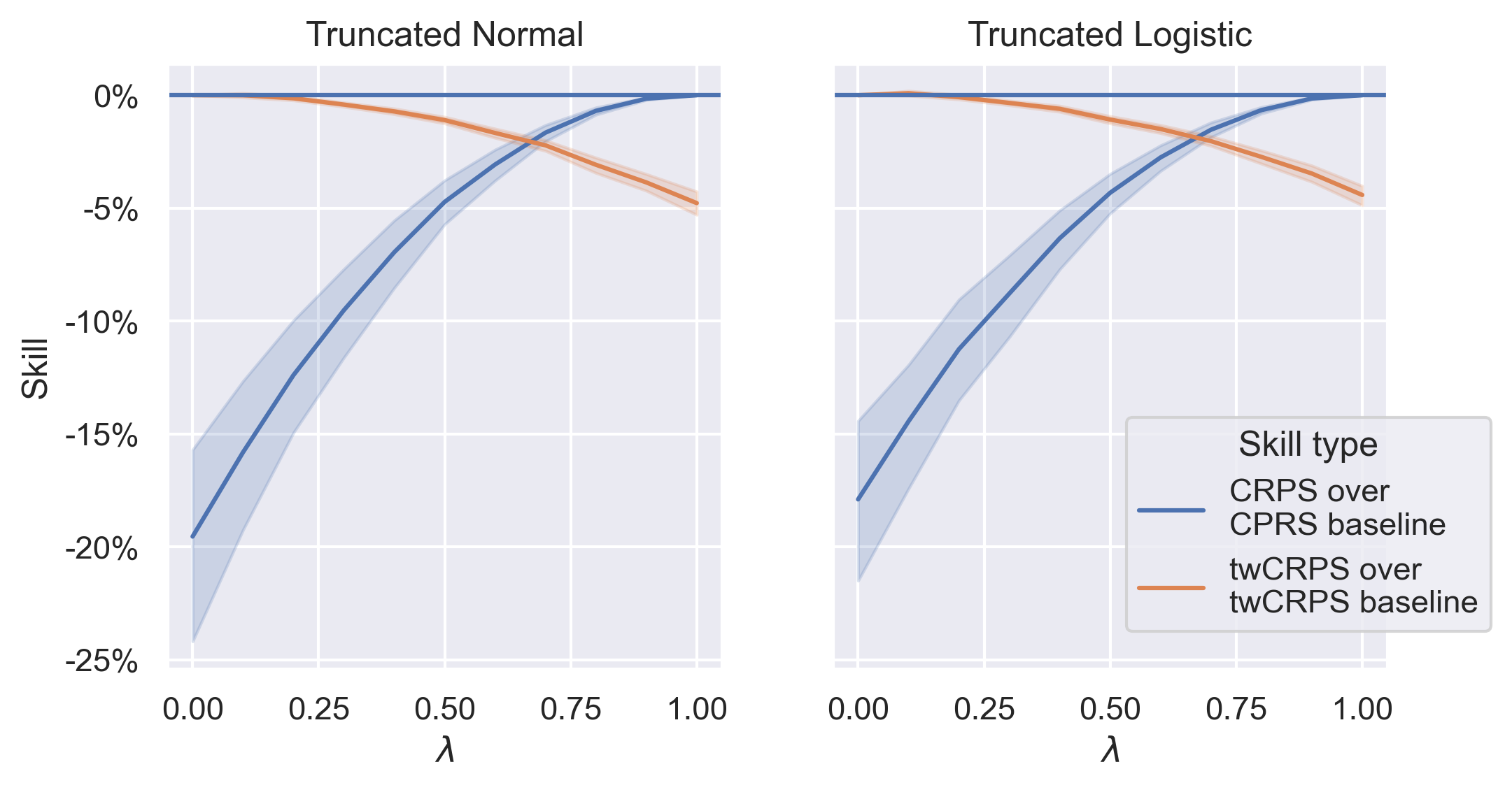
We consider training using weighted scores of the form given in eq. 16. In Figure 6 we show the CRPS skill over the CRPS-trained model (blue) and twCRPS skill over the twCRPS-trained model (orange) for different values of $\gamma$. For $\gamma=0$ the model corresponds to the CRPS-trained model whilst for growing $\gamma$ the twCRPS has stronger influence.

Varying $\gamma$ seems to allow users to control the CRPS loss and twCRPS improvement, with as $\gamma$ grows the resulting model approaching the twCRPS improvement of the twCRPS-trained model and its CRPS loss. Interestingly however, even though the twCRPS for the model with $\gamma=20$ is nearly at the level of the twCRPSt-trained model (at least for the truncated normal distribution), the CRPS skill loss is still much better with only -1.94% CRPS skill loss for the $\gamma=20$ model against -6.35% for the twCRPS-trained models in the truncated normal case and only -2.03% against -11.47% in the truncated logistic case (see section 5.1). Figure 15 in the appendix shows the twCRPS and CRPS for selected values of $\gamma=2,10,20$ for the truncated normal EMOS for both 80th and 90th thresholds. Combining CRPS and twCRPS through weighted training seems to avoid many "outlying" cases where CRPS performance falls off drastically through twCRPS training, whilst still capturing much of the twCRPS improvement. This is similar for the truncated logistic distribution (not shown).

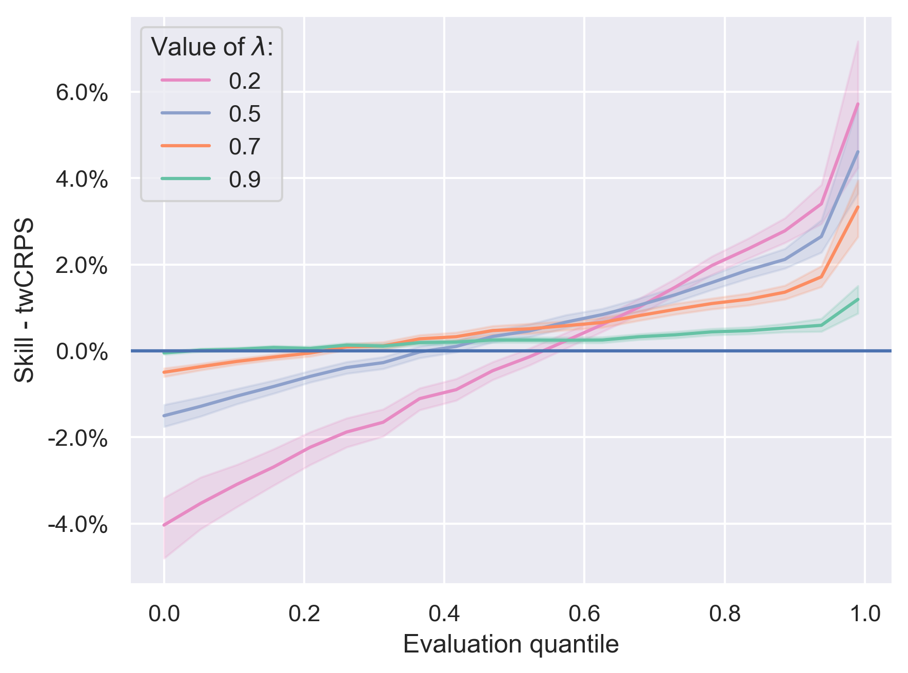
When evaluating the performance of weighted training over a range of evaluation thresholds (figure 16(a) in the appendix for the truncated normal predictive distribution) one finds that the $\gamma$ parameter essentially controls the slope of the curve of twCRPS skill (over the CRPS-trained model): higher values of $\gamma$ lead to forecasts which are worse for the body of the distribution (measured in terms of twCRPS skill for low evaluation quantiles), but better in terms of twCRPS for higher evaluation quantiles, whilst small values of $\gamma$ control the twCRPS loss for small evaluation quantiles much more tightly, but also do not show as substantial of an improvement for high evaluation quantiles.

The parameter $\gamma$ presents a "hyperparameter" that can be chosen by users to tailor a model’s CRPS and twCRPS performance for specific applications. However after training, changing the balance of twCRPS improvement and CRPS loss requires retraining of the post-processing model. Thus in the following we will consider direct combination of CRPS-trained and twCRPS-trained models.

Figure 6: Weighted training: twCRPS skill score over the twCRPS-trained model (orange) and CRPS skill score over the CRPS-trained model (blue) as a function of $\gamma$ for both truncated normal (left) and truncated logistic (right) predictive distributions. The bands represent 95% intervals over stations.

6.2 Linear pool

The $\gamma$ parameter seems to "interpolate" between the CRPS-trained and twCRPS-trained model. We now study combining these models directly using their predictive CDFs. More concretely we study the following convex combination of the predictive distribution functions:

$$F_{\text{pool}}=\lambda F_{\text{CRPS}}+(1-\lambda)F_{\text{twCRPS}}\rightarrow Z_{\text{pool}}\sim\begin{cases}Z_{\text{CRPS}}&\text{ if }U\leq\lambda\\ Z_{\text{twCRPS}}&\text{ if }U>\lambda\end{cases}$$ (17)

where $U\sim\text{Unif}(0,1)$ and $Z_{\text{CRPS}},Z_{\text{twCRPS}}$ follow $F_{\text{CRPS}}$ and $F_{\text{twCRPS}}$ respectively. This is also known as linear pool (Gneiting and Ranjan, 2013; Baran and Lerch, 2018) and the canonical case $\lambda=1/2$ corresponds to simple CDF averaging. The linear pool has some drawbacks, for example Gneiting and Ranjan (2013) show that it necessarily increases dispersion. More advanced versions such as the spread-adjusted linear pool have been proposed, however we defer their study for future work.

We study the twCRPS skill over the twCRPS-trained model and the CRPS skill over the CRPS-trained model, whilst varying $\lambda$ in Figure 7. The $\lambda$ parameter allows to strike a balance between the CRPS (being best for the CRPS-trained model and worst for the twCRPS-trained model) and the twCRPS (vice-versa). The curves are somewhat similar to the ones obtained by weighted training. As one can see the twCRPS improvements and CRPS losses have however very different "steepness", meaning that for example a model with $\lambda=0.6$ still has most of the twCRPS improvements, but controls the majority of the CRPS loss. Evaluating the linear pool over a range of different evaluation quantiles (see figure 16(b) in the appendix for the truncated normal predictive distribution) we find, similar to the weighted training, that the $\lambda$-parameter allows to control the slope of the twCRPS skill curve (over the CRPS-trained model), meaning that for small values of $\lambda$ the twCRPS skill improvement in high quantiles and the twCRPS skill loss in low quantiles is larger, whilst both are smaller for values of $\lambda$ near $1.0$. For different applications different choices of $\lambda$ will be relevant.

Figure 7: Linear pool: twCRPS skill score over the twCRPS-trained model (orange) and CRPS skill score over the CRPS-trained model (blue) as a function of $\lambda$ for both truncated normal (left) and truncated logistic (right) distributions. The bands represent 95% intervals over stations.

We investigate the example case $\lambda=0.6$ for the truncated normal distribution. Figure 8 shows the twCRPS and CRPS skill (relative to the CRPS-trained model) for both the twCRPS-trained and the linear pool model. As one can see the linear pool model keeps much of the twCRPS improvement, but controls the CRPS loss much stronger, with many outlying cases not present. Pooling CRPS-trained and twCRPS-trained models seems to be able to somewhat alleviate the CRPS-twCRPS trade-off.

Figure 8: Linear pool: twCRPS skill score (left) and CRPS skill score (right), both relative to the CRPS-trained model, for the twCRPS and the linear pool model with $\lambda=0.6$. Truncated normal predictive distribution, 80th percentile threshold.

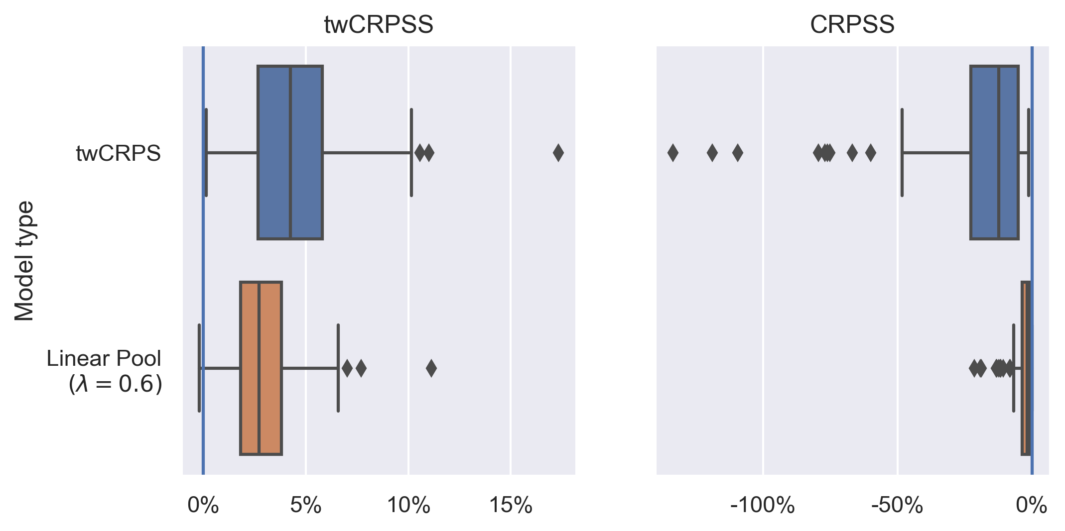
It might be possible to choose the $\lambda$ parameter in a data driven way, possibly based on the ensemble mean or external covariates such as weather patterns (Allen et al., 2021a; Spuler et al., 2024a). Simple experiments parametrizing $\lambda$ in terms of the distance of the ensemble mean to the threshold (a possible measure of the probability of exceedance), however did not show substantial skill over the ad-hoc choice of for example $\lambda=0.6$.

Compared to the weighted training the linear pool directly interpolates between the two models, which means that for low values of $\lambda$ it is able to capture more of the twCRPS improvement, but also has much stronger CRPS loss. The latter is maximal with -1.9% for $\gamma=20$ for the weighted training, whilst reaching -19.5% for $\lambda=0$ in the linear pool case. By choosing adequate values of $\lambda$ and $\gamma$ however it is possible to construct models with very similar twCRPS and CRPS performance using both the linear pool and weighted training. Which one is preferable for applications might therefore depend on individual forecaster’s considerations, most notably whether changing the twCRPS/CRPS balance might be required during application. This would need retraining in the case of weighted training, making the linear pool preferable. For choosing $\gamma$ or $\lambda$ in applications there might be requirements on CRPS/twCRPS performance necessitating specific choices. Otherwise we recommend an ad-hoc choice of a value that somewhat balances the objectives.

7 Interpreting the training impact of the twCRPS

After experiments studying the training of post-processing models using the threshold-weighted CRPS we now consider a number of synthetic experiments to understand the training impact of the twCRPS better in an idealized system. We focus on deriving tail properties from simulated data and on extreme value distributions, which also have been used for various post-processing applications (see for example Baran and Lerch, 2015; Thorarinsdottir et al., 2016), to highlight how using a twCRPS can focus parameter inference on parameters controlling the distribution tail.

7.1 Background: Tail structures and proper scoring rules

Taillardat et al. (2023) argue that the mean (weighted) CRPS cannot distinguish between non-tail-equivalent forecasts. They show that for any random variable $Y$ and any $\nu>0$ it is always possible to construct a non-tail-equivalent random variable $X$ (meaning a random variable with different tail index and thus differing tail behavior/return levels for extremes), such that:

$$|\mathbb{E}_{y\sim Y}\text{wCRPS}(F_{y},y)-\mathbb{E}_{y\sim Y}\text{wCRPS}(F_{x},y)|\leq\nu$$ (18)

where wCRPS is the weighted CRPS with any weighting function $w$. Brehmer and Strokorb (2019) generalise this and show that this is not only a property of the weighted CRPS, but rather all proper scoring rules fail to distinguish between tail equivalent forecasts in the sense of Taillardat et al. (2023). As Brehmer and Strokorb (2019) conclude this casts doubt on the ability of proper scoring rules to distinguish between tail regimes. In practical applications however proper scores such as the log-score (negative log-likelihood) are often successfully used to fit distributions to extremes and to distinguish between tail structures. This is supported by the theory of M-estimation, of which scoring rule inference is a special case (Dawid, 2007), providing consistency guarantees on parameter estimates. Thus the authors of this work believe that the arguments presented in Taillardat et al. (2023) and Brehmer and Strokorb (2019) do not carry conclusive practical implications. This is especially as Taillardat et al. (2023) do not provide bounds on the constructed non-tail-equivalent random variables $X$ that show that these will influence statistical analysis in practice .

Nonetheless we believe Taillardat et al. (2023); Brehmer and Strokorb (2019) highlight an interesting question about the ability of the weighted and especially threshold-weighted CRPS to distinguish between tail regimes. We believe that there is value in studying this question empirically, thus in the following we consider a number of synthetic examples estimating distributions with different tail indices from samples.

7.2 Synthetic experiments

We will consider the following mixture of generalized Pareto distribution ($GPD$) and normal distribution ($N$):

$$Z\sim 0.4\cdot N(\mu,1)+0.6\cdot GPD(0,1,\xi).$$ (19)

Here the $\mu$-parameter controls the location of the distribution body, whilst $\xi$ controls the tail structure. We fix the true $\mu=2$ and $\xi=0.5$. In the following we will consider experiments estimating both parameters using CRPS and twCRPS from 1000 samples of the true model ("training samples"). We consider a grid of candidate values $\hat{\mu},\hat{\xi}$ and for each of these we sample 250 values from the model in equation 19 and compute the sample average CRPS or twCRPS between those samples from the "candidate model" and the 1000 samples from the true model (the "training samples").

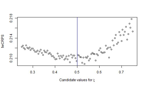
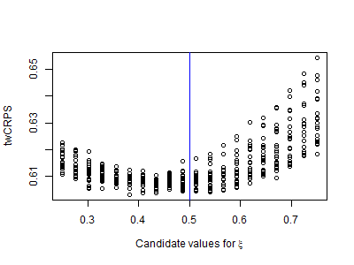
First we fix $\mu=2$ and only estimate the $\xi$ parameter, by varying it between 0.25 and 0.75, shown in Figure 9. All three estimation methods, using CRPS, twCRPS with a threshold based on the 90th percentile and twCRPS with a threshold based on the 95th percentile of the training distribution, seem to be able to stably identify the true tail parameter $\xi=0.5$. Interestingly however the twCRPS with 95th percentile threshold, which following theorem 4.1 effectively censors out 95% of the data seems to be just as stable for estimating $\xi$ as the CRPS. The loss curve seems to have a similar curvature around the minimum and does not seem more "noisy".

(a) CRPS

(b) twCRPS (90th percentile)

(c) twCRPS (95th percentile)

Figure 9: CRPS (a) and twCRPS for 90th (b) and 95th (c) percentile thresholds for different values of $\xi$, with the true $\xi=0.5$ indicated by the blue vertical lines.

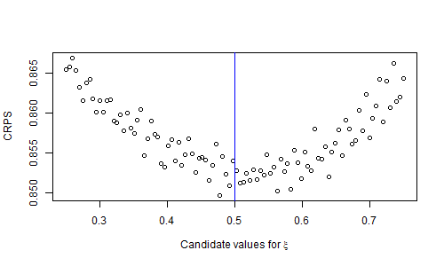
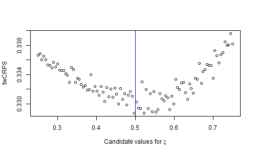
In Figure 10 we estimate both parameters $\mu$ and $\xi$ using the CRPS and twCRPS with a 90th percentile threshold. We plot the CRPS and twCRPS marginally, such that for each value of $\mu$ the CRPS/twCRPS for all candidate values of $\xi$ can be seen and vice-versa. We find that the CRPS is much sharper for the estimation of $\mu$ than it is for the estimation of $\xi$, where the true parameter can’t be identified. This effect seems reversed for the twCRPS which is very inconclusive for $\mu$ estimation, but relatively sharp for the estimation of $\xi$. The twCRPS seems to focus the optimization on the parameter of interest, which controls the tail structure of the synthetic dataset, whilst the CRPS is concentrated on deviations in the body of the distribution.

(a) CRPS for values of $\mu$

(b) CRPS vor values of $\xi$

(c) twCRPS for values of $\mu$

(d) twCRPS for values of $\xi$

Figure 10: CRPS (top, a, b) and twCRPS with 90th percentile threshold (bottom, c, d) for different values of $\mu$ (left, a, c) and $\xi$ (right, b, d). The scatterpoints for each value of $\mu$ and $\xi$ correspond to all values of the respective other parameter. The true $\mu$ and $\xi$ are indicated by the blue vertical lines.

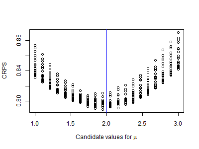
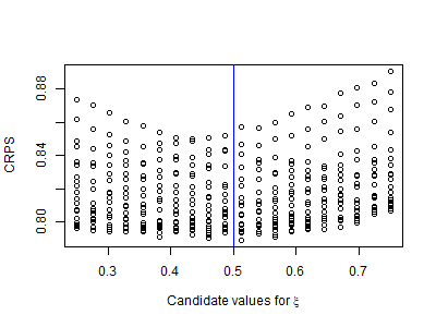
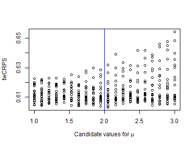
The effect of the twCRPS of focusing inference on the tail structure of a distribution follows mathematically from lemma 4.1. By using the twCRPS with threshold $\tau$ one effectively evaluates the censored CDF using the CRPS, meaning that the body of the distribution only factors in via censoring (the probability mass at the threshold $\tau$ itself). This explains the sharp $\xi$ inference in Figure 10, whilst the $\mu$ inference is inconclusive. For different applications different thresholds can be chosen by users depending on the application. This process of using a CRPS for a censored distribution has some similarities with the usage of censored likelihood in extreme value theory (Huser and Davison, 2014) and it will be interesting to explore the usage of (weighted) proper scores for extreme value inference further in future work (see e.g. Yuen and Stoev 2014 for CRPS based inference in max stable processes and de Fondeville and Davison 2018 for inference using the gradient scoring rule).

8 Discussion and conclusions

In this work we have introduced the usage of threshold-weighted scoring rules to train probabilistic post-processing models, tailored to extremes. This is an alternative to schemes based on weighting loss functions by outcomes which different researchers have been proposing in the literature, which however are problematic as they might encourage "hedging" (Lerch et al., 2017). We have shown the positive effects of training with the twCRPS on forecasts’ extreme event performance. We have identified a distribution body-tail trade-off which manifests as a trade-off between CRPS and twCRPS performance. We have shown that training using a twCRPS is possible for a variety of thresholds of interest and have identified challenges when wanting to optimize sample versions of the twCRPS. We have developed two options for users to balance distribution body and extreme event performance of their forecasts: weighted sums of CRPS and twCRPS and the linear pool between the CRPS and twCRPS forecast. We developed a number of synthetic experiments to show the effect of the twCRPS and finally we have calculated closed-form twCRPS expressions for a number of distributions, which can be found in appendix B together with different characterizations of the twCRPS (appendix A)

We hope that the approaches developed in this article help researchers and operational users to improve forecasts of extreme events, events that are of particular societal relevance. The methodology allows users to choose specific thresholds for which they wish to improve forecasts, which can be relevant for many applications, for example, for airplanes or drones that are only able to operate within certain wind conditions. Given such a threshold, forecasters can use weighted scoring rules to improve distributional forecasts over the threshold. If they are not only interested in extremes they can use either linear pooling or weighted training to balance body and tail forecast performance. The methodology presented has been demonstrated in an application for wind speed, however improving forecasts of extremes (values over a certain impact-relevant threshold) can also be relevant for many other meteorological variables such as temperature and related heat stress or precipitation and precipitation accumulation. The application of the method to these cases is left for future work, however to aid this research we provide closed form twCRPS expressions for many distributions in the appendix.

There are a number of further research questions that follow from this work and should be explored. First it would be interesting to explore the usage of other weighted scores such as the proper quantile weighted score (Gneiting and Ranjan, 2011) or the proper outcome weighted scores (Holzmann and Klar, 2017) and the usage of different, non-threshold-based, weighting functions when training models with weighted scores with emphasis on different parts of the distribution. Allen et al. (2023b, a) develop multivariate versions of the weighted scores, by showing that weighted scores fall into the class of kernel scores. In order to improve predictions of compound extremes – extremes that can have the multiplicity of the impact of singular extremes (Zscheischler et al., 2020) – investigating the usage of these scores to train models with potentially improved forecasting skill for compound extremes might be of interest. This is especially relevant as for example Chen et al. (2022) show the positive effects of a kernelized loss function for improved deterministic predictions of wind speed extremes and similar approaches could be successful for probabilistic predictions. With more complex loss functions or scores, closed-form solutions of these might not be available, thus it might be of interest to investigate how to stabilize sample based optimization of weighted scores. This might also be relevant when it comes to training or finetuning of generative deep learning models, which have shown great potential for post-processing applications (Chen et al., 2024). As neural networks are able to adjust well to large numbers of covariates, this could be combined with research into what predictors for post-processing models are most relevant to improve extreme event forecasts. Research on this and the usage of (weighted) scoring rules for training generative neural networks is in progress by the authors. In addition it might be of interest to investigate forecast combination methods further, for combining distribution body and distribution tail forecasts. For example one could explore methods based on online-learning (van der Meer et al., 2024) or pointwise combinations (Berrisch and Ziel, 2023) and see whether they can help to alleviate the trade-off between CRPS and twCRPS performance further.

Secondly, much more sophisticated post-processing methods exist. Many of these are extensions of EMOS or still based on a closed-form distributional structure, for example so-called distributional regression networks (DRN, Rasp and Lerch 2018) parametrize the parameters of a predictive distribution as neural networks. The authors are hopeful that the results in this article might also generalize to other EMOS-like model structures, however we leave this for future research.

Third and finally, it would be interesting to explore the usage of weighted scoring rules for the training of post-processing models in small training data situations, at longer lead times (Wessel et al., 2024), seasonal to subseasonal time scales or even on climatic timescales for the bias adjustment of climate models (Maraun, 2016; Spuler et al., 2024b), where uncertainties in the prediction of extreme events are even larger and thus the need for probabilistic predictions is even stronger. For these timescales it might also be of interest to explore the usage of extreme value theory informed post-processing methods (Friederichs and Thorarinsdottir, 2012; Lerch and Thorarinsdottir, 2013; Oesting et al., 2017; Velthoen et al., 2019; Taillardat et al., 2019) and explore training of these using threshold-weighted scores, informed by the synthetic experiments in section 7. This is especially relevant as parameter optimization methods, such as the ones explored here, are only one possibility to improve predictive performance of models, next to improvements in the model structure itself. It would be interesting to investigate this trade-off between model structure and estimation further and explore situations and models where threshold-weighted scores might be especially useful for estimation.

Acknowledgements: Jakob Wessel was supported during this work by the Engineering and Physical Sciences Research Council (EPSRC) under grant award number 2696930 and acknowledges support by The Alan Turing Institute’s Enrichment Scheme. The authors would like to thank Sam Allen for pointing out the connection between the threshold-weighted CRPS and the CRPS of a censored distribution, as well as input regarding closed-form expressions of the twCRPS. They are grateful to Jamie Kettleborough and Fiona Spuler for helpful discussions of the results and comments on the manuscript draft.

Code and Data availability: The code for this study can be found at https://github.com/jakobwes/Improving-probabilistic-forecasts-of-extreme-wind-speeds. Unfortunately the authors are unable to share the data, however this can be requested from the UK Met Office.

Appendix A Characterizations and properties of the twCRPS

In the following, to simplify the notation, we make frequent use of the chaining function $v_{s}$ in its canonical form defined as $v_{s}(x):=\max(s,x)$ for $x\in\mathbb{R}$ and $s\in\mathbb{R}$.

Characterization 1: equivalence of the twCRPS and the CRPS of the censored distribution (lemma 4.1 in section 4).

Lemma 4.1.

Let $F$ be a CDF and $y$ an observation. Then

$$\text{twCRPS}_{\tau}(F,y)=\text{CRPS}(\tilde{F}_{\tau},v_{\tau}(y))$$ (20)

where $\tilde{F}_{\tau}$ is the CDF censored at $\tau$:

$$\tilde{F}_{\tau}(x)=\begin{cases}0,&x<\tau,\\ F(x),&x\geq\tau.\end{cases}$$ (21)

Proof.

The proof follows from the definitions of ${\tilde{F}}_{\tau}$ and $v_{\tau}(y)$:

$$\text{CRPS}(\tilde{F}_{\tau},v_{\tau}(y)) =\int_{-\infty}^{\infty}\left[\tilde{F}_{\tau}(z)-\mathbb{1}\left\{z>v_{\tau}(y)\right\}\right]^{2}dz=\int_{\tau}^{\infty}\left[F(z)-\mathbb{1}\left\{z>y\right\}\right]^{2}dz=\text{twCRPS}_{\tau}(F,y)$$ (22)

∎

Characterization 2: expression of the twCRPS through the CRPS and a correction term.

Lemma A.1.

Let $F$ be a CDF and $y$ an observation. Then

$$\text{twCRPS}_{\tau}(F,y)=\text{CRPS}\left(F,v_{\tau}(y)\right)-\Delta_{F}$$ (23)

where $\Delta_{F}$ is a correction term given as

$$\Delta_{F}:=\int_{-\infty}^{\tau}\left[F(z)\right]^{2}dz,$$ (24)

Proof (Lemma A.1).

The proof follows by considering integration limits in the CRPS and twCRPS definitions and the definition of $v_{\tau}(y)$:

$$\text{CRPS}(F,v_{\tau}(y))-\Delta_{F} =\int_{-\infty}^{\tau}\left[F(z)\right]^{2}dz+\int_{\tau}^{v_{\tau}(y)}\left[F(z)\right]^{2}dz+\int_{v_{\tau}(y)}^{\infty}\left[F(z)-1\right]^{2}dz-\int_{-\infty}^{\tau}\left[F(z)\right]^{2}dz$$ (25)

$$=\int_{\tau}^{v_{\tau}(y)}\left[F(z)\right]^{2}dz+\int_{v_{\tau}(y)}^{\infty}\left[F(z)-1\right]^{2}dz$$ (26)

$$=\text{twCRPS}_{\tau}(F,y).$$ (27)

∎

The twCRPS is stable under censoring at a point below the threshold $\tau$:

Lemma A.2.

Let $F$ be a CDF and ${\tilde{F}}_{t}$ be the CDF censored at $t$:

$${\tilde{F}}_{t}(x)=\begin{cases}0,&x<t,\\ F(x),&x\geq t.\end{cases}$$ (28)

Then for $t\leq\tau$:

$$\text{twCRPS}_{\tau}({\tilde{F}}_{t},y)=\text{twCRPS}_{\tau}(F,y)$$ (29)

Proof.

This follows from Lemma 4.1. ∎

The lower-tail twCRPS can be expressed in terms of the CRPS and the upper-tail twCRPS:

Lemma A.3.

The lower-tail twCRPS (for values below instead of above a threshold),

$$\text{twCRPS}_{\tau}^{\text{l}}(F,y):=\int_{-\infty}^{\tau}\left[F(z)-\mathbb{1}\{z\geq y\}\right]^{2}dz$$ (30)

can be expressed in terms of the upper-tail twCRPS as

$$\text{twCRPS}_{\tau}^{\text{l}}(F,y)+\text{twCRPS}_{\tau}^{\text{u}}(F,y)=\text{CRPS}(F,y)$$ (31)

where $\text{twCRPS}_{\tau}^{\text{u}}$ is equal to $\text{twCRPS}_{\tau}$ as used throughout the paper.

Proof.

This follows when considering the integration limits. ∎

Appendix B Closed-form expressions for the twCRPS

We here provide a list of closed-form expressions for the twCRPS for a couple of standard distributions often used in the context of statistical post-processing. Rather than aiming at an exhaustive list, we restrict ourselves to generic cases of the most important distributions. All of the formulae have been verified against numerical integration. In the limit of the threshold $\tau$ moving towards the lower end of the distribution, known expressions for the CRPS are recovered.

Note that the twCRPS is stable under censoring (see Lemma A.2), meaning that all of the closed-form expressions below also apply to censored versions of the distributions if censoring at a point below the threshold $\tau$.

We again make use of the chaining function $v_{s}(x)=\max(s,x)$ for $x\in\mathbb{R}$ and $s\in\mathbb{R}$.

B.1 Distributions supported on the real line

B.1.1 Normal distribution

twCRPS expression:

$$\text{twCRPS}_{\tau}\left(\Phi,y\right)=-\tau\Phi^{2}(\tau)+v_{\tau}(y)\left[2\Phi(v_{\tau}(y))-1\right]+2\left[\varphi(v_{\tau}(y))-\varphi(\tau)\Phi(\tau)\right]-\frac{1}{\sqrt{\pi}}\left[1-\Phi(\sqrt{2}\tau)\right],$$ (32)

$$\text{twCRPS}_{\tau}\left(F_{\mu,\sigma},y\right)=\sigma\,\text{twCRPS}_{(\tau-\mu)/\sigma}\left(\Phi,\frac{y-\mu}{\sigma}\right),$$ (33)

where $\varphi$ and $\Phi$ are the standard normal PDF and CDF, respectively, and $F_{\mu,\sigma}(x)=\Phi\left(\frac{x-\mu}{\sigma}\right)$ with location parameter $\mu\in\mathbb{R}$ and scale parameter $\sigma>0$.

Source: This formula is given by Wessel et al. [2024].

B.1.2 Laplace distribution

twCRPS expression:

$$\text{twCRPS}_{\tau}\left(F,y\right)=\begin{cases}|v_{\tau}(y)|-\frac{3}{4}+\exp(-|v_{\tau}(y)|)-\frac{1}{8}\exp(2\tau),&\tau\leq 0,\\ v_{\tau}(y)-\tau+\exp(-v_{\tau}(y))+\frac{1}{8}\exp(-2\tau)-\exp(-\tau),&\tau\geq 0,\\ \end{cases}$$ (34)

$$\text{twCRPS}_{\tau}\left(F_{\mu,\sigma},y\right)=\sigma\,\text{twCRPS}_{(\tau-\mu)/\sigma}\left(F,\frac{y-\mu}{\sigma}\right),$$ (35)

where $F(x)=\frac{1}{2}+\frac{1}{2}{\rm sgn}(x)[1-\exp(-|x|)]$ is the standard Laplace CDF, and $F_{\mu,\sigma}(x)=F\left(\frac{x-\mu}{\sigma}\right)$ with location parameter $\mu\in\mathbb{R}$ and scale parameter $\sigma>0$.

Source: derived by the authors.

B.1.3 Logistic distribution

twCRPS expression:

$$\text{twCRPS}_{\tau}\left(F,y\right)=F(\tau)-1+\log\frac{1-F(\tau)}{1-F(v_{\tau}(y))}-\log F(v_{\tau}(y)),$$ (36)

$$\text{twCRPS}_{\tau}\left(F_{\mu,\sigma},y\right)=\sigma\,\text{twCRPS}_{(\tau-\mu)/\sigma}\left(F,\frac{y-\mu}{\sigma}\right),$$ (37)

where $F(x)=1/[1+\exp(-x)]$ is the standard logistic CDF, and $F_{\mu,\sigma}(x)=F\left(\frac{x-\mu}{\sigma}\right)$ with location parameter $\mu\in\mathbb{R}$ and scale parameter $\sigma>0$.

Source: This formula is given by Allen et al. [2021b].

B.1.4 Student’s $t$ distribution

twCRPS expression:

$$\begin{aligned} \text{twCRPS}_{\tau}\left(F_{\nu},y\right)=&-\tau F_{\nu}^{2}(\tau)+v_{\tau}(y)\left[2F_{\nu}(v_{\tau}(y))-1\right]\\ &+2\left[F_{\nu}(\tau)G_{\nu}(\tau)-G_{\nu}(v_{\tau}(y))\right]-\bar{B}_{\nu}\left[1-H_{\nu}(\tau)\right],\end{aligned}$$

$$\text{twCRPS}_{\tau}\left(F_{\nu,\mu,\sigma},y\right)=\sigma\,\text{twCRPS}_{(\tau-\mu)/\sigma}\left(F_{\nu},\frac{y-\mu}{\sigma}\right),$$ (38)

where $F_{\nu}$ is the CDF of the Student’s $t$ distribution with $\nu>0$ degrees of freedom, and $F_{\nu,\mu,\sigma}(x)=F_{\nu}\left(\frac{x-\mu}{\sigma}\right)$ with location parameter $\mu\in\mathbb{R}$ and scale parameter $\sigma>0$. Here, $\bar{B}_{\nu}$ and the functions $G_{\nu}$ and $H_{\nu}$ are defined as in Jordan et al. [2019].

Source: derived by the authors. This follows from the CRPS expression for the censored Student’s $t$ distribution in Jordan et al. [2019].

B.2 Distributions with non-negative support

B.2.1 Exponential distribution

twCRPS expression for $\tau\geq 0$:

$$\text{twCRPS}_{\tau}\left(F_{\lambda},y\right)=v_{\tau}(y)-\tau+\frac{2}{\lambda}\left[\exp(-\lambda v_{\tau}(y))-\exp(-\lambda\tau)\right]+\frac{1}{2\lambda}\exp(-2\lambda\tau),$$ (39)

where $F_{\lambda}$ is the CDF of the exponential distribution with rate parameter $\lambda>0$.

Source: derived by the authors.

B.2.2 Gamma distribution

twCRPS expression for $\tau\geq 0$:

$$\text{twCRPS}_{\tau}\left(F_{\alpha,\beta},y\right)= -\tau F_{\alpha,\beta}^{2}(\tau)+v_{\tau}(y)[2F_{\alpha,\beta}(v_{\tau}(y))-1]$$

$$+\frac{\alpha}{\beta}[1-F_{\alpha,\beta}^{2}(\tau)+2F_{\alpha,\beta}(\tau)F_{\alpha+1,\beta}(\tau)-2F_{\alpha+1,\beta}(v_{\tau}(y))]-\frac{1-F_{2\alpha,\beta}(2\tau)}{\beta B\left(\frac{1}{2},\alpha\right)},$$ (40)

where $F_{\alpha,\beta}$ is the CDF of the gamma distribution with shape parameter $\alpha>0$ and rate parameter $\beta>0$, and $B$ denotes the beta function.

Source: derived by the authors.

B.2.3 Log-logistic distribution

twCRPS expression for $\tau\geq 0$ and $0<\sigma<1$:

$$\begin{split}\text{twCRPS}_{\tau}\left(F_{\mu,\sigma},y\right)=&-\tau F_{\mu,\sigma}^{2}(\tau)+v_{\tau}(y)\left[2F_{\mu,\sigma}(v_{\tau}(y))-1\right]\\ &+2\exp(\mu)\left[B_{\rm u}\left(F_{\mu,\sigma}(v_{\tau}(y));1+\sigma,1-\sigma\right)-B_{\rm u}\left(F_{\mu,\sigma}(\tau);2+\sigma,1-\sigma\right)\right],\end{split}$$ (41)

where $F_{\mu,\sigma}$ is the log-logistic CDF with log-location parameter $\mu\in\mathbb{R}$ and log-scale parameter $\sigma>0$, and $B_{\rm u}$ denotes the upper incomplete beta function. The alternative parameterization of the log-logistic distribution in terms of scale parameter $\alpha>0$ and shape parameter $\beta>0$ follows from $\mu=\log\alpha$ and $\sigma=1/\beta$.

Source: derived by the authors.

B.2.4 Log-normal distribution

twCRPS expression for $\tau>0$:

$$\begin{split}\text{twCRPS}_{\tau}\left(F_{\mu,\sigma},y\right)=&-\tau F^{2}_{\mu,\sigma}(\tau)+v_{\tau}(y)[2F_{\mu,\sigma}(v_{\tau}(y))-1]\\ &+2\exp\left(\mu+\frac{1}{2}\sigma^{2}\right)\left[1-F_{\mu+\sigma^{2},\sigma}(v_{\tau}(y))-I\left(\frac{\log\tau-\mu}{\sigma}-\sigma,\sigma\right)\right],\end{split}$$ (42)

where $F_{\mu,\sigma}$ is the CDF of the log-normal distribution with log-location parameter $\mu\in\mathbb{R}$ and log-scale parameter $\sigma>0$.

Here, $I$ is the integral function

$$I(\alpha,\beta)=\int_{\alpha}^{\infty}\varphi(u)\,\Phi(u+\beta)\,du,\hskip 42.67912pt\alpha\in\mathbb{R},\hskip 14.22636pt\beta\in\mathbb{R},$$ (43)

with $\varphi$ and $\Phi$ denoting the standard normal PDF and CDF, respectively. We discuss the evaluation of this integral function in section B.4.

Source: derived by the authors.

B.3 Distributions with flexible support

B.3.1 Continuous uniform distribution on $[a,b]$

twCRPS expression for $a\leq\tau\leq b$ and $a\leq y\leq b$:

$$\text{twCRPS}_{\tau}\left(F,y\right)=\frac{1}{3}\left(1-\tau^{3}\right)+v_{\tau}^{2}(y)-v_{\tau}(y),\qquad 0\leq\tau\leq 1,\qquad 0\leq y\leq 1,$$ (44)

$$\text{twCRPS}_{\tau}\left(F_{a}^{b},y\right)=(b-a)\,\text{twCRPS}_{(\tau-a)/(b-a)}\left(F,\frac{y-a}{b-a}\right),$$ (45)

where $F$ is the CDF of the standard uniform distribution, and $F_{a}^{b}(x)=F\left(\frac{x-a}{b-a}\right)$ with $-\infty<a<b<\infty$.

Source: derived by the authors.

B.3.2 Generalized Pareto distribution

twCRPS expression for $\tau\geq\mu$ and $\xi<1$:

$$\begin{aligned} \text{twCRPS}_{\tau}\left(F_{\xi},y\right)=&v_{\tau}(y)-\tau+\frac{2}{1-\xi}\left\{{\left[1-F_{\xi}(v_{\tau}(y))\right]}^{1-\xi}-{\left[1-F_{\xi}(\tau)\right]}^{1-\xi}\right\}\\ &+\frac{1}{2-\xi}{\left[1-F_{\xi}(\tau)\right]}^{2-\xi},\qquad\qquad\tau\geq 0,\end{aligned}$$

$$\text{twCRPS}_{\tau}\left(F_{\xi,\mu,\sigma},y\right)=\sigma\,\text{twCRPS}_{(\tau-\mu)/\sigma}\left(F_{\xi},\frac{y-\mu}{\sigma}\right),$$ (46)

where $F_{\xi}$ is the CDF of the generalized Pareto distribution with shape parameter $\xi\in\mathbb{R}$, zero location and unit scale, and $F_{\xi,\mu,\sigma}(x)=F_{\xi}\left(\frac{x-\mu}{\sigma}\right)$ with location parameter $\mu\in\mathbb{R}$ and scale parameter $\sigma>0$.

Source: derived by the authors.

B.3.3 Truncated logistic distribution on $[a,b]$

twCRPS expression for $a\leq\tau\leq b$ and $a\leq y\leq b$:

$$\begin{aligned} \text{twCRPS}_{\tau}\left(F_{a}^{b},y\right)=&\frac{1}{[F(b)-F(a)]^{2}}\left\{F(\tau)-F(b)+F^{2}(a)\log\frac{F(v_{\tau}(y))}{F(\tau)}\right.\\ &\left.+[1-F(a)]^{2}\log\frac{1-F(\tau)}{1-F(v_{\tau}(y))}+F^{2}(b)\log\frac{F(b)}{F(v_{\tau}(y))}+[1-F(b)]^{2}\log\frac{1-F(v_{\tau}(y))}{1-F(b)}\right\},\end{aligned}$$

$$\text{twCRPS}_{\tau}\left(F_{a,\mu,\sigma}^{b},y\right)=\sigma\,\text{twCRPS}_{(\tau-\mu)/\sigma}\left(F_{(a-\mu)/\sigma}^{(b-\mu)/\sigma},\frac{y-\mu}{\sigma}\right),$$ (47)

where $F$ is the standard logistic CDF, $F_{a}^{b}$ is the standard logistic CDF truncated to $[a,b]$ with $-\infty<a<b<\infty$, and $F_{a,\mu,\sigma}^{b}(x)=F_{(a-\mu)/\sigma}^{(b-\mu)/\sigma}\left(\frac{x-\mu}{\sigma}\right)$ with location parameter $\mu\in\mathbb{R}$ and scale parameter $\sigma>0$.

For only left truncation ($b\to\infty$), we have:

$$\begin{aligned} \text{twCRPS}_{\tau}\left(F_{a}^{\infty},y\right)=&-\frac{1-F(\tau)}{[1-F(a)]^{2}}+\log\frac{1-F(\tau)}{1-F(v_{\tau}(y))}-\frac{F^{2}(a)}{[1-F(a)]^{2}}\log F(\tau)\\ &-\frac{1+F(a)}{1-F(a)}\log F(v_{\tau}(y)).\end{aligned}$$

Source: For only left truncation, this formula is given by Allen et al. [2021b]; the general case of truncation to $[a,b]$ is derived by the authors.

B.3.4 Truncated normal distribution on $[a,b]$

twCRPS expression for $a\leq\tau\leq b$ and $a\leq y\leq b$:

$$\begin{split}\text{twCRPS}_{\tau}\left(F_{a}^{b},y\right)=&-\tau\left[\frac{\Phi(\tau)-\Phi(a)}{\Phi(b)-\Phi(a)}\right]^{2}+v_{\tau}(y)\left[2\frac{\Phi(v_{\tau}(y))-\Phi(a)}{\Phi(b)-\Phi(a)}-1\right]\\ &+\frac{2}{\Phi(b)-\Phi(a)}\left[\varphi(v_{\tau}(y))-\varphi(\tau)\frac{\Phi(\tau)-\Phi(a)}{\Phi(b)-\Phi(a)}\right]-\frac{1}{\sqrt{\pi}}\frac{\Phi(\sqrt{2}b)-\Phi(\sqrt{2}\tau)}{\left[\Phi(b)-\Phi(a)\right]^{2}},\end{split}$$ (48)

$$\text{twCRPS}_{\tau}\left(F_{a,\mu,\sigma}^{b},y\right)=\sigma\,\text{twCRPS}_{(\tau-\mu)/\sigma}\left(F_{(a-\mu)/\sigma}^{(b-\mu)/\sigma},\frac{y-\mu}{\sigma}\right),$$ (49)

where $F_{a}^{b}$ is the standard normal CDF truncated to $[a,b]$ with $-\infty<a<b<\infty$, and $F_{a,\mu,\sigma}^{b}(x)=F_{(a-\mu)/\sigma}^{(b-\mu)/\sigma}\left(\frac{x-\mu}{\sigma}\right)$ with location parameter $\mu\in\mathbb{R}$ and scale parameter $\sigma>0$. Here, $\varphi$ and $\Phi$ denote the standard normal PDF and CDF, respectively.

The case of only left truncation ($b\to\infty$) follows from $\Phi\left(\frac{b-\mu}{\sigma}\right)=\Phi\left(\frac{\sqrt{2}(b-\mu)}{\sigma}\right)=1$ for any $\mu\in\mathbb{R}$ and $\sigma>0$.

Source: This formula is given by Wessel et al. [2024].

B.4 Some notes on the integral function $I(\alpha,\beta)$

In the derivation of the twCRPS for the log-normal distribution the integral function $I(\alpha,\beta)$ appears (eq.(43)). It has the statistical interpretation as the probability $P(X>\alpha,Y<X+\beta)$ where $X$ and $Y$ are two independent standard normal random variables. The integral function $I$ can be expressed in terms of Owen’s $T$ function [Owen, 1956, 1980],

$$T(h,a)=\frac{1}{2\pi}\int_{0}^{a}\frac{\exp\left[-\frac{1}{2}h^{2}(1+x^{2})\right]}{1+x^{2}},\qquad h\in\mathbb{R},\qquad a\in\mathbb{R},$$ (50)

as

$$I(\alpha,\beta)=\frac{1}{2}\left[\Phi\left(\frac{\beta}{\sqrt{2}}\right)-\Phi(\alpha)\right]+T\left(\alpha,1+\frac{\beta}{\alpha}\right)+T\left(\frac{\beta}{\sqrt{2}},1+\frac{2\alpha}{\beta}\right)+\frac{1}{2}\mathbb{1}\{\alpha\beta<0\},$$ (51)

for $\alpha\neq 0$ and $\beta\neq 0$, and otherwise

$$I(\alpha,0) =\frac{1}{2}[1-\Phi^{2}(\alpha)],$$ (52)

$$I(0,\beta) =\Phi\left(\frac{\beta}{\sqrt{2}}\right)-\frac{1}{2}\Phi^{2}\left(\frac{\beta}{\sqrt{2}}\right).$$ (53)

There are routines available in R and other languages for evaluating Owen’s $T$ function based on various series expansions or numerical integration.

Alternatively, we propose a fast and stable method for evaluating $I(\alpha,\beta)$ based on a recursive power series expansion, making use of (probabilist’s) Hermite polynomials ${\{H_{n}\}}_{n=0}^{\infty}$. The integral function $I$ has the Taylor series

$$I(\alpha,\beta)=\int_{a}^{\infty}\varphi(u)\,\Phi(u+\beta)\,du=\sum_{n=0}^{\infty}I_{n}$$ (54)

where

$$I_{n}=\frac{J_{n}}{n!}\beta^{n}$$ (55)

with

$$J_{0}=I(\alpha,0)=\frac{1}{2}[1-\Phi^{2}(\alpha)]$$ (56)

and

$$J_{n}={\left.\frac{\partial^{n}I}{\partial\beta^{n}}\right|}_{(\alpha,0)}=(-1)^{n-1}\int_{\alpha}^{\infty}H_{n-1}(u)\,\varphi^{2}(u)\,du\qquad n\geq 1.$$ (57)

Using integration by parts and properties of the Hermite polynomials yields the following recursive scheme:

Initialize

$$I_{0}=\frac{1}{2}[1-\Phi^{2}(\alpha)],\quad I_{1}=\frac{\beta}{2\sqrt{\pi}}[1-\Phi(\sqrt{2}\alpha)],\quad I_{2}=-\frac{\beta^{2}}{4}\varphi^{2}(\alpha),$$ (58)

and

$$C_{1}=0,\quad C_{2}=-\frac{\beta^{2}}{4}\varphi^{2}(\alpha),$$ (59)

then iterate:

$$C_{n}= -\frac{\alpha\beta}{n}C_{n-1}-\frac{n-3}{(n-1)n}\beta^{2}C_{n-2},\qquad n\geq 3,$$ (60)

$$I_{n}= C_{n}-\frac{n-2}{2(n-1)n}\beta^{2}I_{n-2},\qquad n\geq 3.$$ (61)

In practice, the power series is truncated after a finite number of terms as soon as $|I_{n}|$ has become small enough. As the recursion may run in two branches of different magnitude involving even and odd indices $n$, respectively, we truncate the series after $N_{*}$ terms where $N_{*}$ is the smallest natural number such that $|I_{N_{*}-1}|<\eta$ and $|I_{N_{*}}|<\eta$ with, say, $\eta={10}^{-15}$. An estimate of the absolute error in $I(\alpha,\beta)$ which turns out to be very close to the actual absolute error can be obtained as

$$\text{err}=\max\left(\eta,\varepsilon\max_{N=0,\dots,N_{*}}\left|\sum_{n=0}^{N}I_{n}\right|\right),$$ (62)

where $\varepsilon$ is the smallest number on the machine, typically $\varepsilon=2^{-52}\approx 2.2\times{10}^{-16}$. In numerical experiments we find that $I(\alpha,\beta)$ is evaluated rather fast and accurately using the above recursion formulas for any $\alpha$ and about $|\beta|<7$. Computation can be further accelerated and the range of tractable values of $\beta$ extended by invoking the identity

$$I(\alpha,\beta)=\Phi\left(\frac{\beta}{\sqrt{2}}\right)-\Phi(\alpha)+I\left(\frac{\beta}{\sqrt{2}},\sqrt{2}\alpha\right)$$ (63)

which is derived using results from Owen [1980]. In summary, our scheme allows to evaluate the twCRPS for the log-normal distribution fast ($N_{\ast}<50$) and virtually to machine precision for any practically relevant combination of parameters $\mu$, $\sigma$ and $\tau$.

Appendix C Reparametrization trick

In section 5.3 we used Adam, a stochastic gradient descent method, to optimize the parameters $\theta$ of the EMOS post-processing model. This requires gradients of the twCRPS-expectation with respect to $\theta$:

$$\nabla_{\theta}\ \text{twCRPS}_{\tau}(F_{\theta},y)=\nabla_{\theta}\left(\mathbb{E}_{X\sim F_{\theta}}|v_{\tau}(X)-v_{\tau}(y)|-\frac{1}{2}\mathbb{E}_{X,X^{\prime}\sim F_{\theta}}|v_{\tau}(X)-v_{\tau}(X^{\prime})|\right).$$ (64)

This is difficult to compute through a Monte-Carlo estimate as the expectations, of which we compute the gradient, also depend on $\theta$. To address this we use the reparametrization trick [Kingma and Welling, 2022] i.e. reparametrize $X\sim F_{\theta}$ as $X=g(\epsilon,\theta)$ with $\epsilon\sim Z$, so in terms of a base-distribution $Z$ which does not depend on the parameters. This allows to write the gradient of the expectation as expectation of a gradient:

$$\nabla_{\theta}\left(\mathbb{E}_{X\sim F_{\theta}}|v_{\tau}(X)-v_{\tau}(y)|-\frac{1}{2}\mathbb{E}_{X,X^{\prime}\sim F_{\theta}}|v_{\tau}(X)-v_{\tau}(X^{\prime})|\right)$$ (65)

$$=\mathbb{E}_{\epsilon\sim Z}\ \nabla_{\theta}\ |v_{\tau}(g(\epsilon,\theta))-v_{\tau}(y)|-\frac{1}{2}\mathbb{E}_{\epsilon,\epsilon^{\prime}\sim Z}\ \nabla_{\theta}\ |v_{\tau}(g(\epsilon,\theta))-v_{\tau}(g(\epsilon^{\prime},\theta))|,$$ (66)

Such a reparametrization is easily possible for the truncated normal and truncated logistic distributions. For example for the truncated normal we sample:

$$g(\epsilon,\mu,\sigma)=\Phi_{\mu,\sigma}^{-1}\left(\Phi_{\mu,\sigma}(0)+\left(1-\Phi_{\mu,\sigma}(0)\right)\cdot\epsilon\right)\text{ with }\epsilon\sim U(0,1),$$ (67)

here $\Phi_{\mu,\sigma}$ is the Gaussian CDF. We use the automatic differentiation integrated in PyTorch [Paszke et al., 2019] to compute exact gradients.

Appendix D Additional experiments for sample-based optimization

We analysed sample based optimization for the truncated normal and truncated logistic distribution for the 80th percentile threshold. As seen above the choice of optimization algorithm and starting values can have a strong influence. Furthermore the choice of the $x_{0}$ parameter in the empirical twCRPS formulation can have an influence on the optimization (see eq. 13, 14). For $x_{0}\neq\tau$ the chaining function is discontinuous, which might impact the optimization, and Allen et al. [2023b] find that in a multivariate example setting $x_{0}=0$ only makes the twCRPS marginally more discriminative than the CRPS for upper tail mis-specifications. We find that using BFGS or Nelder-Mead optimizers the optimization often fails for $x_{0}=0$, but at least for Nelder-Mead sometimes succeeds for $x_{0}=\tau$. The value of $x_{0}$ seems to have less of an impact on the Adam optimizer, however on a subset of stations the resulting models seemed to be less efficient. The difficulty of the choice of $x_{0}$ also has possible impacts for (optimizing) generalizations of the twCRPS to higher dimensions [Allen et al., 2023a, b] where no canonical point (such as $x_{0}=\tau$ here) exists to map all excluded values to.

Figure 11 shows the twCRPS and CRPS skill score (relative to the CRPS-trained model, obtained through closed-form CRPS optimization) for models obtained through minimization of the closed form twCRPS and sample based optimization for Nelder-Mead and Adam optimizers. Training using sample versions is much less efficient i.e. leads to models with far smaller twCRPS improvement than training using the closed-form expressions. Optimization using Nelder-Mead seems to converge, however the resulting models do not improve in terms of twCRPS (and CRPS) over the CRPS baseline, somewhat independently from the number of samples. When using Adam, a stochastic gradient descent algorithm, and exact gradients, sample based optimization seems to work in some cases. However for both optimization algorithms there is a high sensitivity on the starting values. For Adam, when using the parameters from the closed-form CRPS optimization as starting values (in whose neighborhood the twCRPS parameters lie) then the resulting models seems to improve slightly in terms of twCRPS over the CRPS-trained model, without reaching the level of the closed-form-twCRPS-trained model. However using the default starting values, Adam based optimization does not lead to any improvement and is worse in terms of CRPS and twCRPS than the closed-form solution model. For Nelder-Mead CRPS starting values lead to models with the same skill as the CRPS-trained model, whereas the default starting values lead to models that are slightly worse than the CRPS-trained models in terms of both CRPS and twCRPS.

Figure 11: twCRPS and CRPS skill score (over the CRPS-trained model) for models trained using closed form twCRPS solutions as well as the sample twCRPS using different optimizers.

Appendix E Additional figures

(a) 80th percentile

(b) 90th percentile

Figure 12: 80th (a) and 90th (b) percentile of the training distribution used as thresholds. Average 80th percentile threshold: 6.4 m/s (std: 2.1 m/s), maximum 80th percentile threshold: 11.8 m/s. Average 90th percentile threshold: 8.0 m/s std: 2.4 m/s), maximum 90th percentile threshold: 14.4 m/s.

Table 1: Brier skill score (in %) over the CRPS-trained model for the twCRPS-trained model for a variety of evaluation thresholds.

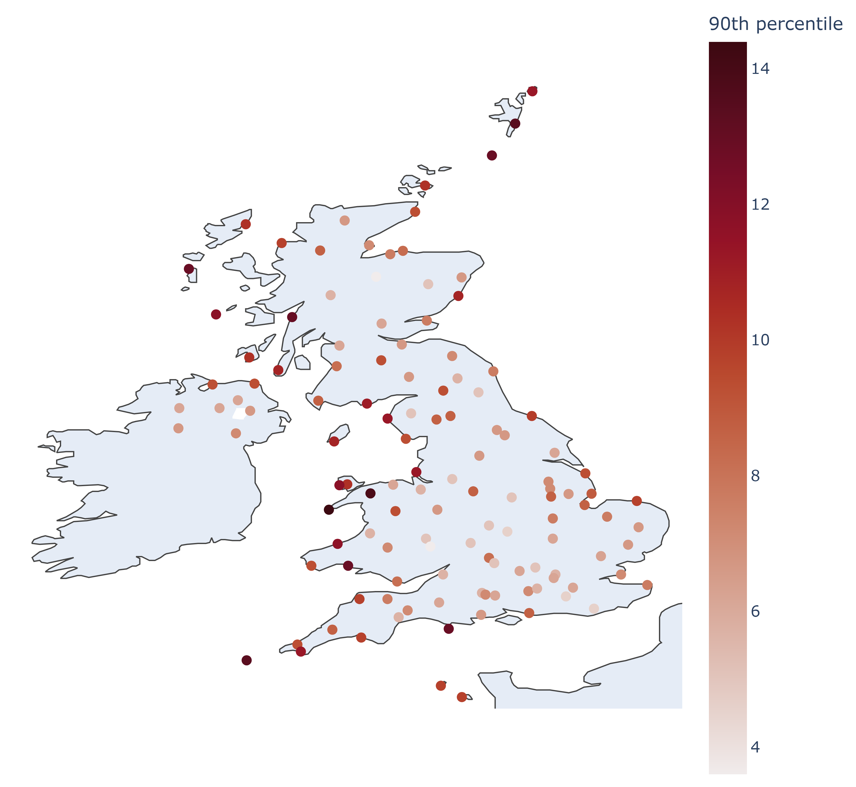
		Truncated Normal	Truncated Logistic
Training Quantile	Evaluation Quantile
0.8	0.7	0.157	0.153
	0.8	1.701	1.624
	0.85	2.300	2.094
	0.9	2.071	2.009
	0.95	1.118	1.091
0.9	0.7	-10.872	-10.928
	0.8	-7.571	-7.859
	0.85	-4.508	-4.578
	0.9	0.936	0.744
	0.95	3.885	3.838

Figure 13: twCRPS skill improvement for the truncated normal twCRPS-trained model and the 90th percentile threshold.

Figure 14: Brier skill score (over the CRPS-trained model) as a function of the threshold for twCRPS-trained models trained using different thresholds. The bands represent 95% intervals over stations.

Figure 15: twCRPS and CRPS for the truncated normal distribution for training using log likelihood, twCRPS and weighted combinations CRPS + $\gamma\cdot$ twCRPS for selected values of $\gamma=2,10,20$.

(a) Weighted Training

(b) Linear Pool

Figure 16: twCRPS skill over the CRPS-trained model for a range of evaluation quantiles for a) models trained using weighted combinations with selected values of $\gamma=2,5,10,20$ and b) linear pool-models for selected values of $\lambda=0.2,0.5,0.7,0.9$. Truncated normal predictive distribution and training threshold as 80th percentile of the training dataset. Note: the twCRPS for an evaluation quantile of 0.0 corresponds to the unweighted CRPS.

References

- Allen et al. [2021a] Sam Allen, Gavin R. Evans, Piers Buchanan, and Frank Kwasniok. Accounting for Skew when Postprocessing MOGREPS-UK Temperature Forecast Fields. Monthly Weather Review, 149(8):2835–2852, August 2021a. ISSN 1520-0493, 0027-0644. doi:10.1175/MWR-D-20-0422.1. URL https://journals.ametsoc.org/view/journals/mwre/149/8/MWR-D-20-0422.1.xml. Publisher: American Meteorological Society Section: Monthly Weather Review.
- Allen et al. [2021b] Sam Allen, Gavin R. Evans, Piers Buchanan, and Frank Kwasniok. Incorporating the North Atlantic Oscillation into the post-processing of MOGREPS-G wind speed forecasts. Quarterly Journal of the Royal Meteorological Society, 147(735):1403–1418, 2021b. ISSN 1477-870X. doi:10.1002/qj.3983. URL https://onlinelibrary.wiley.com/doi/abs/10.1002/qj.3983. _eprint: https://onlinelibrary.wiley.com/doi/pdf/10.1002/qj.3983.
- Allen et al. [2023a] Sam Allen, Jonas Bhend, Olivia Martius, and Johanna Ziegel. Weighted Verification Tools to Evaluate Univariate and Multivariate Probabilistic Forecasts for High-Impact Weather Events. Weather and Forecasting, 38(3):499–516, March 2023a. ISSN 1520-0434, 0882-8156. doi:10.1175/WAF-D-22-0161.1. URL https://journals.ametsoc.org/view/journals/wefo/38/3/WAF-D-22-0161.1.xml. Publisher: American Meteorological Society Section: Weather and Forecasting.
- Allen et al. [2023b] Sam Allen, David Ginsbourger, and Johanna Ziegel. Evaluating Forecasts for High-Impact Events Using Transformed Kernel Scores. SIAM/ASA Journal on Uncertainty Quantification, 11(3):906–940, September 2023b. doi:10.1137/22M1532184. URL https://epubs.siam.org/doi/abs/10.1137/22M1532184. Publisher: Society for Industrial and Applied Mathematics.
- Baran and Lerch [2015] Sándor Baran and Sebastian Lerch. Log-normal distribution based Ensemble Model Output Statistics models for probabilistic wind-speed forecasting. Quarterly Journal of the Royal Meteorological Society, 141(691):2289–2299, 2015. ISSN 1477-870X. doi:10.1002/qj.2521. URL https://onlinelibrary.wiley.com/doi/abs/10.1002/qj.2521. _eprint: https://onlinelibrary.wiley.com/doi/pdf/10.1002/qj.2521.
- Baran and Lerch [2018] Sándor Baran and Sebastian Lerch. Combining predictive distributions for the statistical post-processing of ensemble forecasts. International Journal of Forecasting, 34(3):477–496, July 2018. ISSN 0169-2070. doi:10.1016/j.ijforecast.2018.01.005. URL https://www.sciencedirect.com/science/article/pii/S016920701830030X.
- Baran and Nemoda [2016] Sándor Baran and Dóra Nemoda. Censored and shifted gamma distribution based EMOS model for probabilistic quantitative precipitation forecasting: GAMMA EMOS FOR PRECIPITATION FORECASTING. Environmetrics, 27(5):280–292, August 2016. ISSN 11804009. doi:10.1002/env.2391. URL https://onlinelibrary.wiley.com/doi/10.1002/env.2391.
- Berrisch and Ziel [2023] Jonathan Berrisch and Florian Ziel. CRPS learning. Journal of Econometrics, 237(2, Part C):105221, December 2023. ISSN 0304-4076. doi:10.1016/j.jeconom.2021.11.008. URL https://www.sciencedirect.com/science/article/pii/S0304407621002724.
- Brehmer and Strokorb [2019] Jonas R. Brehmer and Kirstin Strokorb. Why scoring functions cannot assess tail properties. Electronic Journal of Statistics, 13(2):4015–4034, January 2019. ISSN 1935-7524, 1935-7524. doi:10.1214/19-EJS1622. URL https://projecteuclid.org/journals/electronic-journal-of-statistics/volume-13/issue-2/Why-scoring-functions-cannot-assess-tail-properties/10.1214/19-EJS1622.full. Publisher: Institute of Mathematical Statistics and Bernoulli Society.
- Chen et al. [2024] Jieyu Chen, Tim Janke, Florian Steinke, and Sebastian Lerch. Generative machine learning methods for multivariate ensemble postprocessing. The Annals of Applied Statistics, 18(1):159–183, March 2024. ISSN 1932-6157, 1941-7330. doi:10.1214/23-AOAS1784. URL https://projecteuclid.org/journals/annals-of-applied-statistics/volume-18/issue-1/Generative-machine-learning-methods-for-multivariate-ensemble-postprocessing/10.1214/23-AOAS1784.full. Publisher: Institute of Mathematical Statistics.
- Chen et al. [2022] Xi Chen, Ruyi Yu, Sajid Ullah, Dianming Wu, Zhiqiang Li, Qingli Li, Honggang Qi, Jihui Liu, Min Liu, and Yundong Zhang. A novel loss function of deep learning in wind speed forecasting. Energy, 238:121808, January 2022. ISSN 0360-5442. doi:10.1016/j.energy.2021.121808. URL https://www.sciencedirect.com/science/article/pii/S0360544221020569.
- Dawid [2007] A. P. Dawid. The geometry of proper scoring rules. Annals of the Institute of Statistical Mathematics, 59(1):77–93, March 2007. ISSN 1572-9052. doi:10.1007/s10463-006-0099-8. URL https://doi.org/10.1007/s10463-006-0099-8.
- de Fondeville and Davison [2018] Raphaël de Fondeville and Anthony C. Davison. High-dimensional peaks-over-threshold inference. Biometrika, 105(3):575–592, September 2018. ISSN 0006-3444. doi:10.1093/biomet/asy026. URL https://doi.org/10.1093/biomet/asy026.
- Ding et al. [2019] Daizong Ding, Mi Zhang, Xudong Pan, Min Yang, and Xiangnan He. Modeling Extreme Events in Time Series Prediction. In Proceedings of the 25th ACM SIGKDD International Conference on Knowledge Discovery & Data Mining, KDD ’19, pages 1114–1122, New York, NY, USA, July 2019. Association for Computing Machinery. ISBN 978-1-4503-6201-6. doi:10.1145/3292500.3330896. URL https://doi.org/10.1145/3292500.3330896.
- Friederichs and Thorarinsdottir [2012] Petra Friederichs and Thordis L. Thorarinsdottir. Forecast verification for extreme value distributions with an application to probabilistic peak wind prediction. Environmetrics, 23(7):579–594, 2012. ISSN 1099-095X. doi:10.1002/env.2176. URL https://onlinelibrary.wiley.com/doi/abs/10.1002/env.2176. _eprint: https://onlinelibrary.wiley.com/doi/pdf/10.1002/env.2176.
- Friederichs et al. [2018] Petra Friederichs, Sabrina Wahl, and Sebastian Buschow. Chapter 5 - Postprocessing for Extreme Events. In Stéphane Vannitsem, Daniel S. Wilks, and Jakob W. Messner, editors, Statistical Postprocessing of Ensemble Forecasts, pages 127–154. Elsevier, 2018. ISBN 978-0-12-812372-0. doi:https://doi.org/10.1016/B978-0-12-812372-0.00005-4. URL https://www.sciencedirect.com/science/article/pii/B9780128123720000054.
- Gebetsberger et al. [2018] Manuel Gebetsberger, Jakob W. Messner, Georg J. Mayr, and Achim Zeileis. Estimation Methods for Nonhomogeneous Regression Models: Minimum Continuous Ranked Probability Score versus Maximum Likelihood. Monthly Weather Review, 146(12):4323–4338, December 2018. ISSN 1520-0493, 0027-0644. doi:10.1175/MWR-D-17-0364.1. URL https://journals.ametsoc.org/view/journals/mwre/146/12/mwr-d-17-0364.1.xml. Publisher: American Meteorological Society Section: Monthly Weather Review.
- Gneiting and Raftery [2007] Tilmann Gneiting and Adrian E Raftery. Strictly Proper Scoring Rules, Prediction, and Estimation. Journal of the American Statistical Association, 102(477):359–378, March 2007. ISSN 0162-1459. doi:10.1198/016214506000001437. URL https://doi.org/10.1198/016214506000001437. Publisher: Taylor & Francis _eprint: https://doi.org/10.1198/016214506000001437.
- Gneiting and Ranjan [2011] Tilmann Gneiting and Roopesh Ranjan. Comparing Density Forecasts Using Threshold-and Quantile-Weighted Scoring Rules. Journal of Business & Economic Statistics, 29(3):411–422, 2011. ISSN 0735-0015. URL https://www.jstor.org/stable/23243806. Publisher: American Statistical Association.
- Gneiting and Ranjan [2013] Tilmann Gneiting and Roopesh Ranjan. Combining predictive distributions. Electronic Journal of Statistics, 7(none):1747–1782, January 2013. ISSN 1935-7524, 1935-7524. doi:10.1214/13-EJS823. URL https://projecteuclid.org/journals/electronic-journal-of-statistics/volume-7/issue-none/Combining-predictive-distributions/10.1214/13-EJS823.full. Publisher: Institute of Mathematical Statistics and Bernoulli Society.
- Gneiting et al. [2005] Tilmann Gneiting, Adrian E. Raftery, Anton H. Westveld, and Tom Goldman. Calibrated Probabilistic Forecasting Using Ensemble Model Output Statistics and Minimum CRPS Estimation. Monthly Weather Review, 133(5):1098–1118, May 2005. ISSN 1520-0493, 0027-0644. doi:10.1175/MWR2904.1. URL https://journals.ametsoc.org/view/journals/mwre/133/5/mwr2904.1.xml. Publisher: American Meteorological Society Section: Monthly Weather Review.
- Hess and Boers [2022] Philipp Hess and Niklas Boers. Deep Learning for Improving Numerical Weather Prediction of Heavy Rainfall. Journal of Advances in Modeling Earth Systems, 14(3):e2021MS002765, 2022. ISSN 1942-2466. doi:10.1029/2021MS002765. URL https://onlinelibrary.wiley.com/doi/abs/10.1029/2021MS002765. _eprint: https://onlinelibrary.wiley.com/doi/pdf/10.1029/2021MS002765.
- Hess [2020] Reinhold Hess. Statistical postprocessing of ensemble forecasts for severe weather at Deutscher Wetterdienst. Nonlinear Processes in Geophysics, 27(4):473–487, October 2020. ISSN 1023-5809. doi:10.5194/npg-27-473-2020. URL https://npg.copernicus.org/articles/27/473/2020/. Publisher: Copernicus GmbH.
- Holzmann and Klar [2017] Hajo Holzmann and Bernhard Klar. Focusing on regions of interest in forecast evaluation. The Annals of Applied Statistics, 11(4):2404–2431, December 2017. ISSN 1932-6157, 1941-7330. doi:10.1214/17-AOAS1088. URL https://projecteuclid.org/journals/annals-of-applied-statistics/volume-11/issue-4/Focusing-on-regions-of-interest-in-forecast-evaluation/10.1214/17-AOAS1088.full. Publisher: Institute of Mathematical Statistics.
- Huser and Davison [2014] R. Huser and A. C. Davison. Space–Time Modelling of Extreme Events. Journal of the Royal Statistical Society Series B: Statistical Methodology, 76(2):439–461, March 2014. ISSN 1369-7412. doi:10.1111/rssb.12035. URL https://doi.org/10.1111/rssb.12035.
- Jewson et al. [2004] Stephen Jewson, Anders Brix, and Christine Ziehmann. A new parametric model for the assessment and calibration of medium-range ensemble temperature forecasts. Atmospheric Science Letters, 5(5):96–102, 2004. ISSN 1530-261X. doi:10.1002/asl.69. URL https://onlinelibrary.wiley.com/doi/abs/10.1002/asl.69. _eprint: https://onlinelibrary.wiley.com/doi/pdf/10.1002/asl.69.
- Jordan et al. [2019] Alexander Jordan, Fabian Krüger, and Sebastian Lerch. Evaluating Probabilistic Forecasts with scoringRules. Journal of Statistical Software, 90:1–37, August 2019. ISSN 1548-7660. doi:10.18637/jss.v090.i12. URL https://doi.org/10.18637/jss.v090.i12.
- Kingma and Ba [2017] Diederik P. Kingma and Jimmy Ba. Adam: A Method for Stochastic Optimization, January 2017. URL http://arxiv.org/abs/1412.6980. arXiv:1412.6980 [cs].
- Kingma and Welling [2022] Diederik P. Kingma and Max Welling. Auto-Encoding Variational Bayes, December 2022. URL http://arxiv.org/abs/1312.6114. arXiv:1312.6114 [cs, stat].
- Lang et al. [2020] Moritz N. Lang, Sebastian Lerch, Georg J. Mayr, Thorsten Simon, Reto Stauffer, and Achim Zeileis. Remember the past: a comparison of time-adaptive training schemes for non-homogeneous regression. Nonlinear Processes in Geophysics, 27(1):23–34, February 2020. ISSN 1023-5809. doi:10.5194/npg-27-23-2020. URL https://npg.copernicus.org/articles/27/23/2020/. Publisher: Copernicus GmbH.
- Lerch and Thorarinsdottir [2013] Sebastian Lerch and Thordis L. Thorarinsdottir. Comparison of non-homogeneous regression models for probabilistic wind speed forecasting. Tellus A: Dynamic Meteorology and Oceanography, 65(1):21206, December 2013. ISSN 1600-0870. doi:10.3402/tellusa.v65i0.21206. URL http://a.tellusjournals.se/article/10.3402/tellusa.v65i0.21206/. Number: 1 Publisher: Stockholm University Press.
- Lerch et al. [2017] Sebastian Lerch, Thordis L. Thorarinsdottir, Francesco Ravazzolo, and Tilmann Gneiting. Forecaster’s Dilemma: Extreme Events and Forecast Evaluation. Statistical Science, 32(1):106–127, February 2017. ISSN 0883-4237, 2168-8745. doi:10.1214/16-STS588. URL https://projecteuclid.org/journals/statistical-science/volume-32/issue-1/Forecasters-Dilemma-Extreme-Events-and-Forecast-Evaluation/10.1214/16-STS588.full. Publisher: Institute of Mathematical Statistics.
- Maraun [2016] Douglas Maraun. Bias Correcting Climate Change Simulations - a Critical Review. Current Climate Change Reports, 2(4):211–220, December 2016. ISSN 2198-6061. doi:10.1007/s40641-016-0050-x. URL https://doi.org/10.1007/s40641-016-0050-x.
- Messner et al. [2022] Jakob Messner, Achim Zeileis, and Reto Stauffer. crch: Censored Regression with Conditional Heteroscedasticity, September 2022. URL https://CRAN.R-project.org/package=crch.
- Messner et al. [2014] Jakob W. Messner, Georg J. Mayr, Daniel S. Wilks, and Achim Zeileis. Extending Extended Logistic Regression: Extended versus Separate versus Ordered versus Censored. Monthly Weather Review, 142(8):3003–3014, August 2014. ISSN 1520-0493, 0027-0644. doi:10.1175/MWR-D-13-00355.1. URL https://journals.ametsoc.org/view/journals/mwre/142/8/mwr-d-13-00355.1.xml. Publisher: American Meteorological Society Section: Monthly Weather Review.
- Nelder and Mead [1965] J. A. Nelder and R. Mead. A Simplex Method for Function Minimization. The Computer Journal, 7(4):308–313, January 1965. ISSN 0010-4620. doi:10.1093/comjnl/7.4.308. URL https://doi.org/10.1093/comjnl/7.4.308.
- Nocedal and Wright [2006] Jorge Nocedal and Stephen J. Wright. Numerical Optimization. Springer Series in Operations Research and Financial Engineering. Springer New York, 2006. ISBN 978-0-387-30303-1. doi:10.1007/978-0-387-40065-5. URL http://link.springer.com/10.1007/978-0-387-40065-5.
- Oesting et al. [2017] Marco Oesting, Martin Schlather, and Petra Friederichs. Statistical post-processing of forecasts for extremes using bivariate brown-resnick processes with an application to wind gusts. Extremes, 20(2):309–332, June 2017. ISSN 1572-915X. doi:10.1007/s10687-016-0277-x. URL https://doi.org/10.1007/s10687-016-0277-x.
- Olivetti and Messori [2024] Leonardo Olivetti and Gabriele Messori. Advances and prospects of deep learning for medium-range extreme weather forecasting. Geoscientific Model Development, 17(6):2347–2358, March 2024. ISSN 1991-959X. doi:10.5194/gmd-17-2347-2024. URL https://gmd.copernicus.org/articles/17/2347/2024/. Publisher: Copernicus GmbH.
- Owen [1980] D. B. Owen. A table of normal integrals. Communications in Statistics - Simulation and Computation, 9(4):389–419, January 1980. ISSN 0361-0918. doi:10.1080/03610918008812164. URL https://doi.org/10.1080/03610918008812164. Publisher: Taylor & Francis _eprint: https://doi.org/10.1080/03610918008812164.
- Owen [1956] Donald B. Owen. Tables for Computing Bivariate Normal Probabilities. The Annals of Mathematical Statistics, 27(4):1075–1090, December 1956. ISSN 0003-4851, 2168-8990. doi:10.1214/aoms/1177728074. URL https://projecteuclid.org/journals/annals-of-mathematical-statistics/volume-27/issue-4/Tables-for-Computing-Bivariate-Normal-Probabilities/10.1214/aoms/1177728074.full. Publisher: Institute of Mathematical Statistics.
- Paszke et al. [2019] Adam Paszke, Sam Gross, Francisco Massa, Adam Lerer, James Bradbury, Gregory Chanan, Trevor Killeen, Zeming Lin, Natalia Gimelshein, Luca Antiga, Alban Desmaison, Andreas Köpf, Edward Yang, Zach DeVito, Martin Raison, Alykhan Tejani, Sasank Chilamkurthy, Benoit Steiner, Lu Fang, Junjie Bai, and Soumith Chintala. PyTorch: An Imperative Style, High-Performance Deep Learning Library, December 2019. URL http://arxiv.org/abs/1912.01703. arXiv:1912.01703 [cs, stat].
- Porson et al. [2020] Aurore N. Porson, Joanne M. Carr, Susanna Hagelin, Rob Darvell, Rachel North, David Walters, Kenneth R. Mylne, Marion P. Mittermaier, Steve Willington, and Bruce Macpherson. Recent upgrades to the Met Office convective-scale ensemble: An hourly time-lagged 5-day ensemble. Quarterly Journal of the Royal Meteorological Society, 146(732):3245–3265, 2020. ISSN 1477-870X. doi:10.1002/qj.3844. URL https://onlinelibrary.wiley.com/doi/abs/10.1002/qj.3844. _eprint: https://onlinelibrary.wiley.com/doi/pdf/10.1002/qj.3844.
- Rasp and Lerch [2018] Stephan Rasp and Sebastian Lerch. Neural Networks for Postprocessing Ensemble Weather Forecasts. Monthly Weather Review, 146(11):3885–3900, November 2018. ISSN 1520-0493, 0027-0644. doi:10.1175/MWR-D-18-0187.1. URL https://journals.ametsoc.org/view/journals/mwre/146/11/mwr-d-18-0187.1.xml. Publisher: American Meteorological Society Section: Monthly Weather Review.
- Roberts et al. [2023] Nigel Roberts, Benjamin Ayliffe, Gavin Evans, Stephen Moseley, Fiona Rust, Caroline Sandford, Tomasz Trzeciak, Paul Abernethy, Laurence Beard, Neil Crosswaite, Ben Fitzpatrick, Jonathan Flowerdew, Tom Gale, Leigh Holly, Aaron Hopkinson, Katharine Hurst, Simon Jackson, Caroline Jones, Ken Mylne, Christopher Sampson, Michael Sharpe, Bruce Wright, Simon Backhouse, Mark Baker, Daniel Brierley, Anna Booton, Clare Bysouth, Robert Coulson, Sean Coultas, Ric Crocker, Roger Harbord, Kathryn Howard, Teresa Hughes, Marion Mittermaier, Jon Petch, Tim Pillinger, Victoria Smart, Eleanor Smith, and Mark Worsfold. IMPROVER: The New Probabilistic Postprocessing System at the Met Office. Bulletin of the American Meteorological Society, 104(3):E680–E697, March 2023. ISSN 0003-0007, 1520-0477. doi:10.1175/BAMS-D-21-0273.1. URL https://journals.ametsoc.org/view/journals/bams/104/3/BAMS-D-21-0273.1.xml. Publisher: American Meteorological Society Section: Bulletin of the American Meteorological Society.
- Scheepens et al. [2023] Daan R. Scheepens, Irene Schicker, Kateřina Hlaváčková-Schindler, and Claudia Plant. Adapting a deep convolutional RNN model with imbalanced regression loss for improved spatio-temporal forecasting of extreme wind speed events in the short to medium range. Geoscientific Model Development, 16(1):251–270, January 2023. ISSN 1991-959X. doi:10.5194/gmd-16-251-2023. URL https://gmd.copernicus.org/articles/16/251/2023/. Publisher: Copernicus GmbH.
- Scheuerer and Möller [2015] Michael Scheuerer and David Möller. Probabilistic wind speed forecasting on a grid based on ensemble model output statistics. The Annals of Applied Statistics, 9(3):1328–1349, September 2015. ISSN 1932-6157, 1941-7330. doi:10.1214/15-AOAS843. URL https://projecteuclid.org/journals/annals-of-applied-statistics/volume-9/issue-3/Probabilistic-wind-speed-forecasting-on-a-grid-based-on-ensemble/10.1214/15-AOAS843.full. Publisher: Institute of Mathematical Statistics.
- Sharpe [2022] Michael Sharpe. A colourful world of weather: representing local climatology in forecasts. Weather, 77(3):83–87, 2022. ISSN 1477-8696. doi:10.1002/wea.3901. URL https://onlinelibrary.wiley.com/doi/abs/10.1002/wea.3901. _eprint: https://onlinelibrary.wiley.com/doi/pdf/10.1002/wea.3901.
- Sharpe and Stewart [2019] Michael Sharpe and Emily Stewart. Verification of Postprocessed Summer Temperature Forecasts at U.K. Sites Using Observed Climate-Based Thresholds. Weather and Forecasting, 34(3):715–730, June 2019. ISSN 1520-0434, 0882-8156. doi:10.1175/WAF-D-18-0157.1. URL https://journals.ametsoc.org/view/journals/wefo/34/3/waf-d-18-0157_1.xml. Publisher: American Meteorological Society Section: Weather and Forecasting.
- Sharpe et al. [2018] Michael A. Sharpe, Clare E. Bysouth, and Rebecca L. Stretton. How well do Met Office post-processed site-specific probabilistic forecasts predict relative-extreme events? Meteorological Applications, 25(1):23–32, 2018. ISSN 1469-8080. doi:10.1002/met.1665. URL https://onlinelibrary.wiley.com/doi/abs/10.1002/met.1665. _eprint: https://onlinelibrary.wiley.com/doi/pdf/10.1002/met.1665.
- Spuler et al. [2024a] Fiona Raphaela Spuler, Marlene Kretschmer, Yevgeniya Kovalchuk, Magdalena Alonso Balmaseda, and Theodore G. Shepherd. Identifying probabilistic weather regimes targeted to a local-scale impact variable, February 2024a. URL http://arxiv.org/abs/2402.15379. arXiv:2402.15379 [physics].
- Spuler et al. [2024b] Fiona Raphaela Spuler, Jakob Benjamin Wessel, Edward Comyn-Platt, James Varndell, and Chiara Cagnazzo. ibicus: a new open-source Python package and comprehensive interface for statistical bias adjustment and evaluation in climate modelling (v1.0.1). Geoscientific Model Development, 17(3):1249–1269, February 2024b. ISSN 1991-959X. doi:10.5194/gmd-17-1249-2024. URL https://gmd.copernicus.org/articles/17/1249/2024/. Publisher: Copernicus GmbH.
- Taillardat et al. [2019] Maxime Taillardat, Anne-Laure Fougères, Philippe Naveau, and Olivier Mestre. Forest-Based and Semiparametric Methods for the Postprocessing of Rainfall Ensemble Forecasting. Weather and Forecasting, 34(3):617–634, June 2019. ISSN 1520-0434, 0882-8156. doi:10.1175/WAF-D-18-0149.1. URL https://journals.ametsoc.org/view/journals/wefo/34/3/waf-d-18-0149_1.xml. Publisher: American Meteorological Society Section: Weather and Forecasting.
- Taillardat et al. [2023] Maxime Taillardat, Anne-Laure Fougères, Philippe Naveau, and Raphaël de Fondeville. Evaluating probabilistic forecasts of extremes using continuous ranked probability score distributions. International Journal of Forecasting, 39(3):1448–1459, July 2023. ISSN 0169-2070. doi:10.1016/j.ijforecast.2022.07.003. URL https://www.sciencedirect.com/science/article/pii/S0169207022001017.
- Thorarinsdottir and Gneiting [2010] Thordis L. Thorarinsdottir and Tilmann Gneiting. Probabilistic forecasts of wind speed: ensemble model output statistics by using heteroscedastic censored regression. Journal of the Royal Statistical Society: Series A (Statistics in Society), 173(2):371–388, 2010. ISSN 1467-985X. doi:10.1111/j.1467-985X.2009.00616.x. URL https://onlinelibrary.wiley.com/doi/abs/10.1111/j.1467-985X.2009.00616.x. _eprint: https://onlinelibrary.wiley.com/doi/pdf/10.1111/j.1467-985X.2009.00616.x.
- Thorarinsdottir and Schuhen [2018] Thordis L. Thorarinsdottir and Nina Schuhen. Chapter 6 - Verification: Assessment of Calibration and Accuracy. In Stéphane Vannitsem, Daniel S. Wilks, and Jakob W. Messner, editors, Statistical Postprocessing of Ensemble Forecasts, pages 155–186. Elsevier, 2018. ISBN 978-0-12-812372-0. doi:https://doi.org/10.1016/B978-0-12-812372-0.00006-6. URL https://www.sciencedirect.com/science/article/pii/B9780128123720000066.
- Thorarinsdottir et al. [2016] Thordis L. Thorarinsdottir, Michael Scheuerer, and Christopher Heinz. Assessing the Calibration of High-Dimensional Ensemble Forecasts Using Rank Histograms. Journal of Computational and Graphical Statistics, 25(1):105–122, January 2016. ISSN 1061-8600. doi:10.1080/10618600.2014.977447. URL https://doi.org/10.1080/10618600.2014.977447. Publisher: Taylor & Francis _eprint: https://doi.org/10.1080/10618600.2014.977447.
- van den Goorbergh et al. [2022] Ruben van den Goorbergh, Maarten van Smeden, Dirk Timmerman, and Ben Van Calster. The harm of class imbalance corrections for risk prediction models: illustration and simulation using logistic regression. Journal of the American Medical Informatics Association, 29(9):1525–1534, September 2022. ISSN 1527-974X. doi:10.1093/jamia/ocac093. URL https://doi.org/10.1093/jamia/ocac093.
- van der Meer et al. [2024] Dennis van der Meer, Pierre Pinson, Simon Camal, and Georges Kariniotakis. CRPS-based online learning for nonlinear probabilistic forecast combination. International Journal of Forecasting, January 2024. ISSN 0169-2070. doi:10.1016/j.ijforecast.2023.12.005. URL https://www.sciencedirect.com/science/article/pii/S0169207023001371.
- Velthoen et al. [2019] Jasper Velthoen, Juan-Juan Cai, Geurt Jongbloed, and Maurice Schmeits. Improving precipitation forecasts using extreme quantile regression. Extremes, 22(4):599–622, December 2019. ISSN 1572-915X. doi:10.1007/s10687-019-00355-1. URL https://doi.org/10.1007/s10687-019-00355-1.
- Velthoen et al. [2023] Jasper Velthoen, Clément Dombry, Juan-Juan Cai, and Sebastian Engelke. Gradient boosting for extreme quantile regression. Extremes, 26(4):639–667, December 2023. ISSN 1572-915X. doi:10.1007/s10687-023-00473-x. URL https://doi.org/10.1007/s10687-023-00473-x.
- Walters et al. [2017] David Walters, Ian Boutle, Malcolm Brooks, Thomas Melvin, Rachel Stratton, Simon Vosper, Helen Wells, Keith Williams, Nigel Wood, Thomas Allen, Andrew Bushell, Dan Copsey, Paul Earnshaw, John Edwards, Markus Gross, Steven Hardiman, Chris Harris, Julian Heming, Nicholas Klingaman, Richard Levine, James Manners, Gill Martin, Sean Milton, Marion Mittermaier, Cyril Morcrette, Thomas Riddick, Malcolm Roberts, Claudio Sanchez, Paul Selwood, Alison Stirling, Chris Smith, Dan Suri, Warren Tennant, Pier Luigi Vidale, Jonathan Wilkinson, Martin Willett, Steve Woolnough, and Prince Xavier. The Met Office Unified Model Global Atmosphere 6.0/6.1 and JULES Global Land 6.0/6.1 configurations. Geoscientific Model Development, 10(4):1487–1520, April 2017. ISSN 1991-959X. doi:10.5194/gmd-10-1487-2017. URL https://gmd.copernicus.org/articles/10/1487/2017/. Publisher: Copernicus GmbH.
- Wessel et al. [2024] Jakob Benjamin Wessel, Christopher A. T. Ferro, and Frank Kwasniok. Lead-time-continuous statistical postprocessing of ensemble weather forecasts. Quarterly Journal of the Royal Meteorological Society, n/a(n/a), January 2024. ISSN 1477-870X. doi:10.1002/qj.4701. URL https://onlinelibrary.wiley.com/doi/abs/10.1002/qj.4701. _eprint: https://onlinelibrary.wiley.com/doi/pdf/10.1002/qj.4701.
- Williams et al. [2014] R. M. Williams, C. A.T. Ferro, and F. Kwasniok. A comparison of ensemble post-processing methods for extreme events. Quarterly Journal of the Royal Meteorological Society, 140(680), 2014. ISSN 1477870X. doi:10.1002/qj.2198.
- Yuen and Stoev [2014] Robert Yuen and Stilian Stoev. CRPS M-estimation for max-stable models. Extremes, 17(3):387–410, September 2014. ISSN 1572-915X. doi:10.1007/s10687-014-0185-x. URL https://doi.org/10.1007/s10687-014-0185-x.
- Zscheischler et al. [2020] Jakob Zscheischler, Olivia Martius, Seth Westra, Emanuele Bevacqua, Colin Raymond, Radley M. Horton, Bart van den Hurk, Amir AghaKouchak, Aglaé Jézéquel, Miguel D. Mahecha, Douglas Maraun, Alexandre M. Ramos, Nina N. Ridder, Wim Thiery, and Edoardo Vignotto. A typology of compound weather and climate events. Nature Reviews Earth and Environment, 1(7), 2020. ISSN 2662138X. doi:10.1038/s43017-020-0060-z.