Mini-Sequence Transformer: Optimizing Intermediate Memory for Long Sequences Training

Abstract

We introduce Mini-Sequence Transformer (MsT), a simple and effective methodology for highly efficient and accurate LLM training with extremely long sequences. MsT partitions input sequences and iteratively processes mini-sequences to reduce intermediate memory usage. Integrated with activation recomputation, it enables significant memory savings in both forward and backward passes. In experiments with the Llama3-8B model, with MsT, we measure no degradation in throughput or convergence even with 12x longer sequences than standard implementations due to our careful memory optimizations. MsT is fully general, implementation-agnostic, and requires minimal code changes to integrate with existing LLM training frameworks.

1 Introduction

The development of Transformer [52] has been a remarkable journey, with each iteration pushing the boundaries of what is possible regarding model size, performance, and efficiency. One of the critical challenges in this journey has been managing the memory requirements of these models, particularly during training. As Transformers have significantly grown in size[8] and complexity [39], the memory demand has increased exponentially, necessitating innovative solutions to optimize memory usage while maintaining performance.

A significant milestone in this journey was the introduction of multi-query attention [45]. This technique dramatically reduced the size of the KV-cache during inference, which uses multiple query heads but single key and value heads. The idea was first adopted in the large-scale training of PaLM [10], then adopted and empirically tested in LLaMA [51]. As the field progressed, multi-query attention evolved into grouped query attention (GQA) [3], which relaxes the single key and value head restriction to multiple heads, and each head is coupled with a group of queries. It significantly improves the quality and is adopted by Llama2-70B [51] and Mistral-7B [21].

To further improve model quality, Llama3 [33] introduced a tokenizer with a vocabulary of 128K tokens, enabling more efficient language encoding than Llama2’s 32K vocabulary. Additionally, Llama3 increased its MLP intermediate size from 11k to 14k. These changes reflect a trend toward more extensive vocabulary and intermediate sizes for better quality. Meanwhile, Llama3 maintains its hidden size of 4k for inference efficiency. This trend is also reflected in the Microsoft development of Phi-3 [2] compared with Phi-2 [20].

These advancements have also brought about new memory challenges, particularly in the intermediate value of linear layers of multilayer perception(MLP) and language modeling head (LM-Head). The substantial increase in intermediate variables, which can be nearly ten times larger than the input variables, has severely limited the network’s ability to expand sequence length and batch size. This limitation has made it difficult to train large models without restricting sequence length to 8K or relying on gradient accumulation or distributed systems to expand batch size.

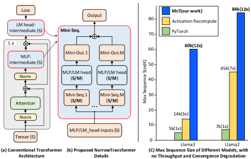
Our Approach: Recognizing these challenges, we introduce Mini-Sequence Transformer (MsT), a simple and effective methodology for enabling highly efficient and highly accurate LLM training with extremely long sequence lengths by reducing intermediate memory overhead. MsT introduces a per-layer mini-sequence where the input partitions work for each MLP and LM-Head block. MsT partitions individual samples along the sequence dimension and iteratively processes each mini-sequence, combining all mini-sequence results to recover full-sequence outputs for these blocks. Our work also adopts activation recomputation [6]. We find that there is no degradation in throughput or convergence even with sequences up to $12\times$ compared to a standard implementation of Llama3-8B, as shown in Figure 1(c). This is achieved by optimizing the intermediate memory of activation.

Figure 1: (a) Standard Transformer architecture. MLP’s and LM-Head’s activation sequence length is annotated with $S$. (b) Mini-Sequence Transformer is used to replace MLP blocks and LM-Head block, which splits the input sequence $S$ into $M$ mini-sequences with sequence length $S/M$, where $M=2$ on this figure. (c) Max sequence size for training Llama2/Llama3 on A100-80GB GPU, with no degradation of throughput or convergence using our approach.

To summarize, we make the following contributions to advance the state-of-the-art in long-sequence training:

• MsT trains 12x longer sequence lengths than existing systems on a single A100 GPU with no degradation in throughput and convergence of training.

• Fully general and implementation agnostic: MsT supports most parameter-efficient training as it works independently with attention layers.

• Support for large-scale distributed training: MsT works together with DeepSpeed-Ulysses [19] to support linear scaling sequence length by the number of GPUs.

• Easy-to-use and portable, requiring minimal code changes to the existing training frameworks.

In subsequent sections, we provide background and related work, a detailed discussion of Mini-Sequence Transformer (MsT) design, Hardware-efficient analysis, experimental evaluation, and comparison with existing work. This work is open-source on https://github.com/wdlctc/mini-s under an MIT license.

2 Background and Related Work

This section briefly overviews the performance characteristics of long sequence transformers on modern hardware(e.g., GPUs). We also describe some background of mini-batch training, which inspires our work.

2.1 Transformer Architecture

Figure 1(a) is a sketch of the building blocks of a typical Transformer architecture [52]. It consists of input sequences $S$ sent into $L$ repeated block with attention and MLP, then computed output loss with LM-Head block. The inputs and outputs of each block are typically a 3D tensor of size $(B,S,d)$ where $B$ is micro batch size, $S$ is sequence length, and $d$ is hidden dimension. The intermediate value includes the $Q,K,V$ tensors of size $(B,S,d)$ within the attention block, the $I$ tensor of size $(B,S,I)$ within the MLP block, and the logits tensor of size $(B,S,V)$ of within LM-Head block. Here, $I$ represents the intermediate size of MLP, and $V$ represents the vocabulary size.

2.2 Hardware Performance of Long Sequence Training

Memory Hierarchy. GPUs have a memory hierarchy with larger but slower global GPU memory (high bandwidth memory; HBM) and smaller but faster-shared memory (SRAM). This high memory demand originates from the quadratic complexity of self-attention operations, where the memory needed to store attention scores for each token increases quadratically as the sequence length grows. This dramatic increase in memory demand can quickly overwhelm the capacity of the HBM, leading to OOM issues. Flashattention [13] uses kernel fusion to effectively mitigate the memory overheads associated with the quadratic growth in sequence length, and Xformer [36] deploys optimized memory access patterns that achieve linear memory scaling. Our work is partly inspired by memory optimization technologies, where our optimization targets are MLP and LM-Head.

Occupancy. GPUs have many threads executed in parallel; threads are grouped into thread blocks, which execute on streaming multiprocessors (SMs). Modern hardware has specialized units like tensor cores on NVIDIA GPU to accelerate mammals. In long sequence training scenarios where the sequence size tends to be long (>10k), parallelizing over the sequence dimension usually enables high GPU occupancy.

Performance characteristics. GPU operators can be classified as either compute-bound or memory-bound, which is determined by the time spent in arithmetic operations and the time spent accessing HBM. Typical self-attention with long sequence, MLP with the long intermediate size is a compute-bound operator because their core operators are matrix-multiply with a large inner dimension of sequence length. Then, cross-entropy with reduction is memory-bound.

2.3 Mini-Batch Training

Our work is inspired by Mini-Batch Training algorithms, also known as gradient accumulation. Mini-batch training algorithms [14] were initially designed for training variance reduction. It updates models toward an average of multiple gradients and reduces the variance to speed up the convergence. Then, Mini-Batch Training is discovered to support large batch size by processing the training batch in smaller mini-batches, which allows the model to be trained on a subset of the data at a time, accumulating gradients over several mini-batch and only updating the parameter with accumulated gradient [16, 35].

This reduces the memory requirements compared to batch gradient descent [22], which enables training bigger batch sizes than GPU memory constrain. We are inspired by the idea and adapt it to train long sequences instead of large batch sizes.

3 Mini-Sequence Transformer (MsT): Algorithm, Analysis, and Distributed Extensions

We present our Mini-Sequence Transformer (MsT) mechanism with the idea of partitioning the input sequence into $M\times$ mini-sequences. We show how to compute the exact transformer block by storing small intermediate matrices for the backward pass. Then, we analyze its IO complexity, showing that our method is throughput-equalized compared to the standard transformer. We further show how MsT can work on distributed settings by integrating with DeepSpeed [19].

We focus here on the forward pass for ease of exposition; Appendix B contains details for the backward. These implementations are partially inspired by Triton [49] and Transformer in Triton [1].

3.1 Algorithms: Reducing Intermediate Value With Mini-Sequence Processing

Our idea arises from the observation of large intermediate values from transformer blocks. Given the inputs $X\in\mathbb{R}^{N\times d}$ in HBM, attention blocks and MLP blocks compute the output $O\in\mathbb{R}^{N\times d}$ and loss computation block computes the output $loss\in\mathbb{R}^{1}$, $N$ equals to sequence size $S$ here. We observe that the intermediate values are always larger than the input $X$ and output $O$, $loss$, illustrated in Table 1. Attention has intermediate values $\mathbf{Q},\mathbf{K},\mathbf{V}\in\mathbb{R}^{N\times d}$, which is $(1+2\times d)/G$ larger than input size, where $(1+2\times d/G=1.5)$ in Llama3 setting. MLP has intermediate value $I_{up},I_{gate}\in\mathbb{R}^{N\times I}$, where $2\times I/d=16$ in Llama3 setting. LM-Head has $logits\in\mathbb{R}^{V\times d}$, where $V/d=32$ in Llama3 setting. The detail setting of Llama3-8B is listed in Appendix C

Table 1: Intermediate value size analysis for transformer blocks

Transformer Blocks	Input/Output Size	Peak Intermediate Value Size	Ratio Intermediate/Input
Attention	$(B,S,d)/(B,S,d)$	$(B,S,d)+2\times(B,S,d/G)$	$(1+2\times d)/G$
MLP	$(B,S,d)/(B,S,d)$	$2\times(B,S,I)$	$(2\times I)/d$
LM-Head	$(B,S,d)/1$	$(B,S,V)$	$V/d$

As flash attention and group query attention have minimized the intermediate value of attention, we put our focus on the MLP block and LM-Head block. Therefore, our implementation of MsT is general enough to work with any attention: self-attention [52], cross-attention [4], causal attention [37], their sparse counterparts [9, 55, 43], and their various optimized kernels such as different versions of FlashAttention [13, 12]. Our implementation adopts FlashAttention2 [12] for the experiments.

Input Partition.

We apply the mini-sequence technique to overcome the technical challenge of large intermediate values occupying HBM memory. We describe this in Algorithms 1, and 2, which represent MLP blocks and LM-Head from Llama2 [51] and Llama3[33]. Their MLP block consists of three linear layers and SiLU function [41], and their LM-Head block consists of one linear layer and CrossEntropyLoss function[44]. The corresponding backward implementations can be referred to in Appendix B for more details. The main idea is to partition the input $X$ into mini-sequence $X_{i}$ as Algorithm 1 line 1 and Algorithm 2 line 1, then compute the output with respect to those mini-sequences. We get the exact same result as standard implementation by contacting all mini-sequence outputs.

Gradient Accumulation.

One of our goals is to reduce intermediate values for backward passes. The backward pass typically requires the matrices $X\in\mathbb{R}^{N\times d}$, $I\in\mathbb{R}^{N\times I}$, $logits\in\mathbb{R}^{N\times V}$ to compute the gradients with respect to weights. However, by input partition the $X\in\mathbb{R}^{N_{m}\times d}$, we can reduce the intermediate value as $I\in\mathbb{R}^{N_{m}\times I}$, $logits\in\mathbb{R}^{N_{m}\times V}$ by $M\times$ in the backward pass in HBM. With gradient accumulation for all mini-sequences, all gradients are generated in the same way as standard implementation by introducing more memory loading time. However, as MLP is the standard computation-bound operator and LM-Head occupies only a small amount of total training time, MsT would not affect the whole training speed with a significant reduction in memory overhead.

Algorithm 1 Mini-Sequence MLP

0:  Matrices $X\in\mathbb{R}^{N\times d}$, Weights $W_{gate},W_{up}\in\mathbb{R}^{d\times I}$, $W_{down},\in\mathbb{R}^{I\times d}$

1:  Partition matrices $X$ into $M$ blocks $X_{1},\dots,X_{m}$ of size $N_{m}\times d$, where $N_{m}=N/M$

2:  for $1\leq i\leq M$ do

3:     Compute $I_{i}^{\prime}=SiLU((X_{i}W_{gate})*(X_{i}W_{up}))$, $I_{i}\in\mathbb{R}^{N_{m}\times I}$

4:     Compute $\mathbf{O}_{i}^{\prime}=I_{i}W_{down}$, $\mathbf{O}_{i}\in\mathbb{R}^{N_{m}\times d}$

5:  end for

6:  Contact $\mathbf{O}=\{\mathbf{O}_{i},\dots,\mathbf{O}_{m}\}\in\mathbb{R}^{N\times d}$

7:  Return $\mathbf{O}$.

Algorithm 2 Mini-Sequence LM-Head

0:  Matrices $X\in\mathbb{R}^{N\times d}$, Labels $L\in\mathbb{R}^{N}$, Weights $W_{out}\in\mathbb{R}^{d\times V}$

1:  Partition matrices $X$ into $M$ blocks $X_{1},\dots,X_{m}$ of size $N_{m}\times d$, where $N_{m}=N/M$

2:  Partition labels $L$ into $M$ sub-label, $L_{1},\dots,L_{m}$ of size $N_{m}$, where $N_{m}=N/M$

3:  for $1\leq i\leq M$ do

4:     Compute $logits_{i}=X_{i}W_{out}$, $logits_{i}\in\mathbb{R}^{N_{m}\times V}$

5:     Compute if $(i-1)*N_{m}\leq L_{i}\leq(i-1)*N_{m}$, $L_{i}=L_{i}$ else $L_{i}=-100$

6:     Compute $loss_{i}=crossentropyloss(logits_{i},L\_)$

7:  end for

8:  Compute $loss=\sum_{1}^{M}loss_{i}/M$

9:  Return $loss$.

3.2 Analysis: IO Complexity of Mini-Sequence Transformer (MsT)

We analyze the IO complexity of MsT, compared with consistent compute complexity, which can affect its compute-bound or memory-bound performance characteristics.

Theorem 1.

Let $S$ be the sequence length, $d$ be the hidden dimension, $I$ be the intermediate size, and $V$ be the voice size. Standard MLP returns $O=act((XW_{gate})*(X_{i}W_{up}))*W_{down}$ with $O(SdI)$ FLOPS and MsT MLP returns $O(SdI/M*M)=O(SdI)$ FLOPS. Standard LM-Loss returns $loss=crossentropyloss(XW,L)$ with $O(SdV+SV)$ FLOPS, and MsT LM-Loss returns $O((SdV+SV)/M*M)=O(SdV+SV)$ FLOPS.

Theorem 2.

Standard MLP requires $\Theta(Sd+SI+dI)$ HBM accesses, while MsT (1) requires $\Theta(Sd+SI+dIM)$ HBM accesses. Standard LM-Head requires $\Theta(Sd+SV+dV)$ HBM accesses, while MsT (2) requires $\Theta(Sd+SV+dVM)$ HBM accesses.

For Llama3 values of $d$ (4096), $I$ (14336) and $V$ (128256), $SI$, $Sv$ is many time larger than $Sd$. For long sequence cases like $S=100k,S>>d$, the compute complexity and IO complexity are dominated by $SI$ and $SV$, where MsT is close to standard implementation. In this scenario, the intermediate value can be saved by $M\times$ while maintaining the same throughput performance. However, for small sequence cases where $S<<d$, the compute complexity and IO complexity are dominated by $dI$ and $dV$ while MsT needs $dIM$ and $dVM$. Therefore, MsT would cause throughput downgrades.

Figure 2: Distributed Mini-Sequence Transformer.

3.3 Extension: Distributed Mini-Sequence Transformer (MsT)

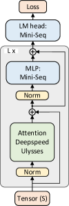
We extend Mini-Sequence Transformer (MsT) to the distributed setting: we propose MsT +Deepspeed-Ulpysis, which can effectively scale the transformer using sequence parallelism(SP). In SP, the input tensor of each Transformer layer is divided along the sequence dimension, allowing for parallel computation across multiple GPUs. This segmentation, in conjunction with activation recomputation, results in a substantial reduction in activation memory requirements. It is worth noting that our proposed approach is orthogonal to most sequence parallelism, such as Megatron-LM [23], Deepspeed-Ulysses [19], Sequence parallelism [28], and Ring Attention [29]. Here, we take Deepspeed-Ulysses as an example of how they work together.

Figure 2 shows the design of extending MsT with DeepSpeed-Ulysses. As with the transformers architecture, the design consists of an attention block with DeepSpeed-Ulysses, MLP, and LM-Head with MsT’s mini-sequence technology. The design consists of input sequences $S$ partitioned across $P$ available devices and mini-sequence using $M$. Each attention block Matrices $\mathbf{Q},\mathbf{K},\mathbf{V}$ are communicated through all-to-all collectives before and after the attention computation. The remaining modules of MLP and LM-Head use the sequence parallel and mini-sequence together. As DeepSpeed-Ulysses’s main change is working on attention block and MsT is working on MLP and LM-Head, it is straightforward to make them work together to scale sequence length.

4 Experiment

We evaluate the impact of using Mini-Sequence Transformer (MsT) on Llama3[33], a state-of-the-art model for many NLP tasks. We validate our claims about scaling sequence length, reporting training time, and memory overhead. Distributed Extension results can be found in appendix E, which confirms that the sequence length of MsT can scale linearly with the number of GPUs.

• Maximun Sequence Length. MsT scales transformer to longer sequences. MsT can train Llama3-8B with context length 60k and Llama3-7B with context length 84k on a single A100 GPU. MsT outperforms the activation recomputation sequence length by $1.8-4\times$ for Llama3-8B, Llama2-7B and Llama2-13b, and it achieves $12-20\times$ than standard implementation.

• Training throughput. MsT maintains the same training throughput compared with standard long-sequence training.

4.1 Longer Sequence Length with Mini-Sequence Transformer (MsT)

Llama3.

We train a Llama3-8B[33] MsT by exploring the sequence length on a single A100 GPU with lossless training strategies, such as activation recomputation and MsT. Lossy strategies like sliding windows [11] and LoRA [17] are not included in our experiments. Table 2 compares our maximum sequence and training time to the PyTorch standard implementation and Huggingface PEFT with activation recomputation. Our implementation trains $4\times$ longer sequence compared with activation recomputation and $12\times$ longer sequence compared with standard implementation.

Table 2: Maximum sequence length of Llama3-8B, running on single A100 80G GPU.

Llama3-8B-hf Implementation	Maximum Sequence Length (K)
Llama3-8B-hf vanilla	5
Llama3-8B-hf activation recomputation	14
Llama3-8B-hf MsT	60

Llama2.

We also train Llama2 models[38] with MsT, in order to compare the performance of MsT on different models. Table 3 compares our maximum sequence to the PyTorch standard implementation and Huggingface PEFT with activation recomputation. Our implementation trains $1.8\times$ longer sequence compared with activation recomputation and $12\times$ longer sequence compared with standard implementation.

Table 3: Maximum sequence length of Llama2 models, running on single A100 80G GPU.

Model Implementation	Maximum Sequence Length (K)
Llama2-7B-hf Huggingface 4.40.1	7
Llama2-7B-hf Huggingface PEFT	45
Llama2-7B-hf MsT	84
Llama2-13B-hf Huggingface 4.40.1	2
Llama2-13B-hf Huggingface PEFT	25
Llama2-13B-hf MsT	40

Combination with gradient accumulation.

Gradient Accumulation has been used during training Llama2 and Llama3, which helps them train larger batch sizes given limited available GPU memory. However, in Gradient Accumulation, instead of updating the model parameters after processing each batch of training data, the gradients are accumulated over multiple batches before updating. This means that the memory usage for gradients would occupy the memory used for activation. Therefore, using gradient accumulation during training would significantly constrain the maximum sequence size.

Table 4 summarizes the maximum sequence length with gradient accumulation. The activation recomputation technology can train up to 8K sequences, which happens to be the default setting of Llama3 training. Then MsT can train up to 30k sequence length, which is $3.75\times$ longer sequence length compared with activation recomputation plus gradient accumulation. MsT can also scale $1.3\times$ sequence for Llama2-7B’s training

Table 4: Maximum sequence length training on single A100 80G GPU with gradient accumulation.

Llama3-8B-hf Implementation with gradient accumulation	Maximum Sequence Length (K)
Llama3-8B-hf activation recomputation	8
Llama3-8B-hf MsT	30
Llama2-7B-hf activation recomputation	38
Llama2-7B-hf MsT	52

4.2 Faster Long Sequence Training with Mini-Sequence Transformer (MsT)

We evaluate the training performance of MsT on Llama3-8B and Llama2-7B models using a single A100 80G GPU. Table 5 compares the training time per step and TFLOPS achieved by MsT with the vanilla PyTorch implementation and activation recomputation technique from Hugging Face PEFT.

Table 5: Training performance using MsT on single A100 80G GPU.

Model Implementation	Batch Size	Training Time Per Step (s)	TFLOPS
Llama3-8B-hf vanilla	1	OOM	OOM
Llama3-8B-hf activation recomputation	2	5.01	3271.42
Llama3-8B-hf MsT	2	5.80	2825.12
Llama3-8B-hf MsT	8	19.64	3336.14
Llama2-7B-hf vanilla	1	1.24	3290.88
Llama2-7B-hf activation recomputation	8	8.85	3703.48
Llama2-7B-hf MsT	8	9.49	3452.19
Llama2-7B-hf MsT	16	18.00	3639.93

For Llama3-8B, the vanilla implementation runs out of memory (OOM) with a batch size of 1. Activation recomputation allows training with a batch size of 2, achieving 3271.42 TFLOPS and a training time of 5.01 seconds per step. MsT, with the same batch size of 2, achieves a comparable 2825.12 TFLOPS with a slightly longer training time of 5.80 seconds per step. However, MsT’s memory efficiency allows scaling the batch size to 8, resulting in an improved 3336.14 TFLOPS and a training time of 19.64 seconds per step.

In the case of Llama2-7B, the vanilla implementation can train with a batch size of 1, achieving 3290.88 TFLOPS and a training time of 1.24 seconds per step. Activation recomputation enables a batch size of 8, yielding 3703.48 TFLOPS and a training time of 8.85 seconds per step. MsT further increases the batch size to 16, maintaining a similar 3639.93 TFLOPS with a training time of 18.00 seconds per step.

4.3 Better Models with Longer Sequences

Language Modeling with Long Context.

The memory efficiency of MsT allows us to increase the context length of llama by $4\times$ than activation recomputation. Table 6 shows that LLAMA3 with MsT and context 30K achieves 1.35 better perplexity than the activation recomputation method. We train a Llama3-8B[33] MsT on the LongAlpaca dataset[7], with an average sequence of 16k. The training lasts for one epoch for demonstration. For all implementation, we use the AdamW optimizer [31]. We use a weight decay of 0.001, gradient clipping of 1.0, and a constant learning rate of 1e-4. All batch sizes equal 16, with a gradient accumulation step of 16. The bf16 precision is also deployed.

Table 6: LLAMA2-7b with MsT, with 4x larger context length compared to activation recomputation.

Llama3-8B-hf Implementation	Context length	LongAlpaca (ppl)	loss	Training Time
Llama3-8B-hf activation recomputation	8k	290.0	5.67	7.5 hours
Llama3-8B-hf MsT	8k	301.9	5.71	7.6 hours
Llama3-8B-hf MsT	16k	240.3	5.48	21.5 hours
Llama3-8B-hf MsT	30k	222.4	5.40	62.9 hours

Training Curve with MsT.

We show that MsT is a pure system optimization technique that enables extreme long sequence Transformer model training. Thus, there is no negative on the quality of trained models; this assertion is validated through experiments shown in Figure 3. We train a Llama3-8B[33] MsT on the Long-Data-Collections dataset[50]. The Long-Data-Collections dataset is a compilation of extrame long context datasets specifically designed for tasks requiring extensive comprehension and inference from large text inputs.

Figure 3. (a) shows the convergence evaluation for the Llama3-8B model with 8k. We plot the training loss over 1000 steps for the baseline transformer (blue curve) and MST (orange curve). The learning curves are nearly identical, confirming that applying the mini-sequence technique in MST does not degrade model quality. Similarly, Figure 3. (b) presents the convergence evaluation for the Llama3-8B model with 30k, the Maximum sequence length training on a single A100 80G GPU with gradient accumulation. Again, we observe that the training loss curves MST converge well when all baselines fail to run because of out-of-memory.

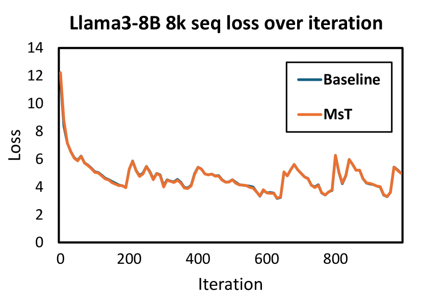
(a) Convergence evaluation of Llama3-8B with 8k sequence length.

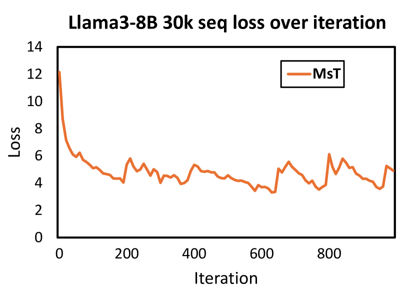
(b) Convergence evaluation of Llama3-8B with 30k sequence length.

Figure 3: Convergence evaluation of MsT. Training

5 Ablation Study:

5.1 Memory Optimization of Mini-Sequence Transformer (MsT)

MsT introduces a series of memory optimizations to reduce the memory overhead of long-sequence training. To understand the effectiveness of MsT memory optimizations, we perform an ablation study that incrementally turns off these optimizations (mini-sequence, activation recomputation) and measures the memory requirements. We consider three options: vanilla (standard Pytorch with BF16), activation recomputation only, and MsT with activation recomputation.

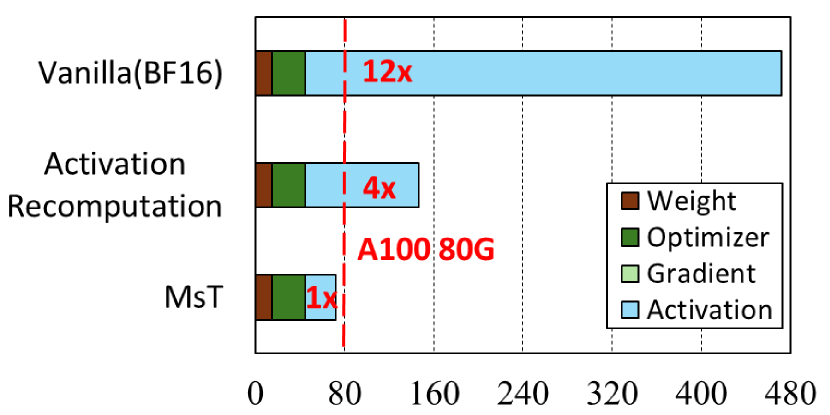
(a) Memory consumption of pre-training Llama3-8B with 20k context.

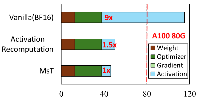
(b) Memory consumption of pre-training Llama2-7B with 20k context.

Figure 4: Memory consumption of pre-training Llama3-8B and Llama2-7B models with a token batch size of 1 on a single A100 device, with activation recomputation and MsT. Note that long-sequence training gradients overlap with activation, so gradients are not shown in bars.

Figure 4 shows the results. We analyze the peak memory usage of Llama3-8B and Llama2-7B, with a sequence length of 20k. For sequence length 20k of Llama2-7B, MsT and activation recomputation can make the model fit into A100 GPU, while for Llama3-8B, only MsT can make the model fit. The rest of the memory consumption is estimated based on its model architectures and theoretical activation amount. For Llama3, activation recomputation can reduce the memory overhead of activation by 3x, and MsT can further reduce 4x memory overhead based on activation recomputation. Activation recomputation works better for training Llama2 because the intermediate value is much less for this model, with 6x activation memory saving. MsT achieves 9x memory saving, which can be improved for the longer sequence to 12x. Combining them, they can reduce 12x activation memory overhead. More detail on the ablation study of memory can be found in Appendix D.

5.2 How many mini-sequences are needed during pre-training

We observe that increasing $M$, the number of mini-sequence blocks, can help with memory efficiency, but it has certain limitations. As shown in 5, MsT can significantly benefit memory usage with minimal impact on training speed. The reason has been discussed in Sec 3.2, since in the long sequence training case, the modeling processing is significantly computed-bound while using mini-sequence would not make it memory-bound, providing much space for memory usage optimization. Figure 5(a,c) show the time per step remains relatively stable as M increases for both the MLP and LM-Head, indicating throughput is maintained. Figure 5(b,d) shows the peak memory decreases as M increases, demonstrating the memory savings from partitioning into more mini-sequences. Therefore, in terms of balancing memory efficiency and computational performance, we use M=4 for the MLP and M=16 for the LM-Head. The details data and analysis can be found in Appendix F.

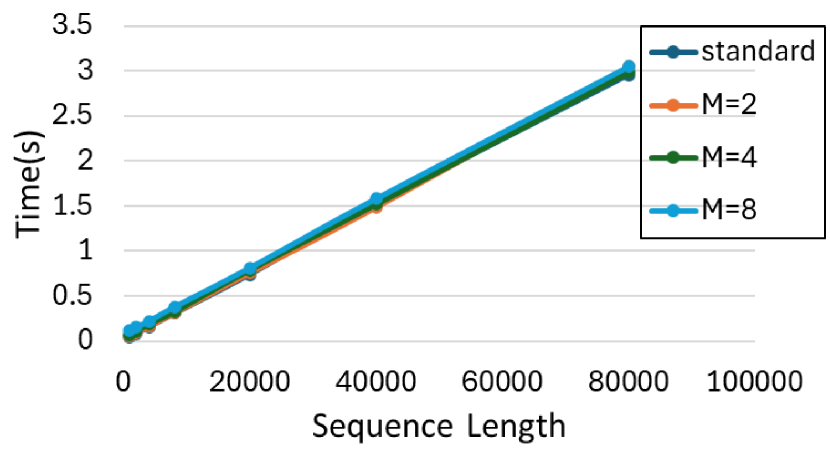
(a) Time per step for Llama3-8B MLP.

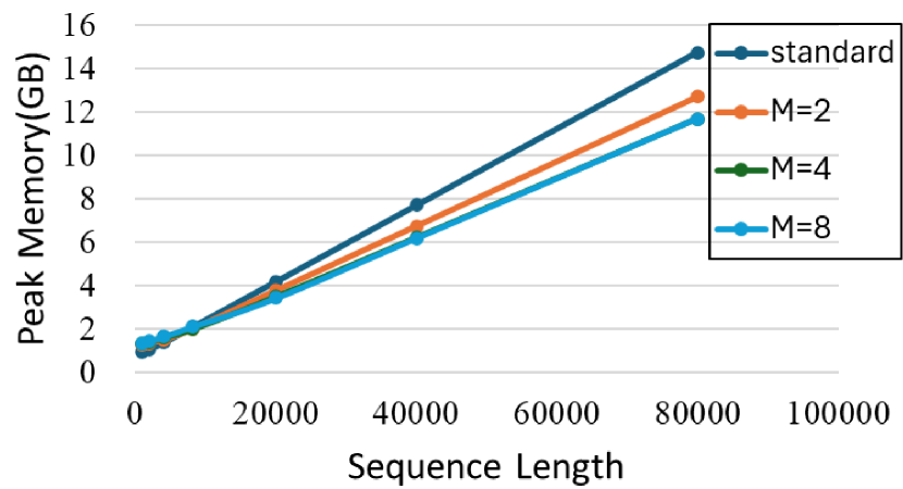
(b) Peak Memory for Llama3-8B MLP.

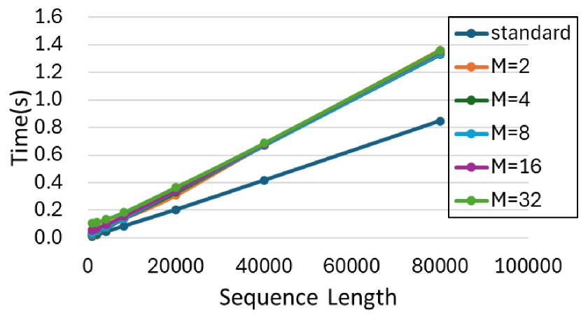
(c) Time per step for Llama3-8B LM-Head.

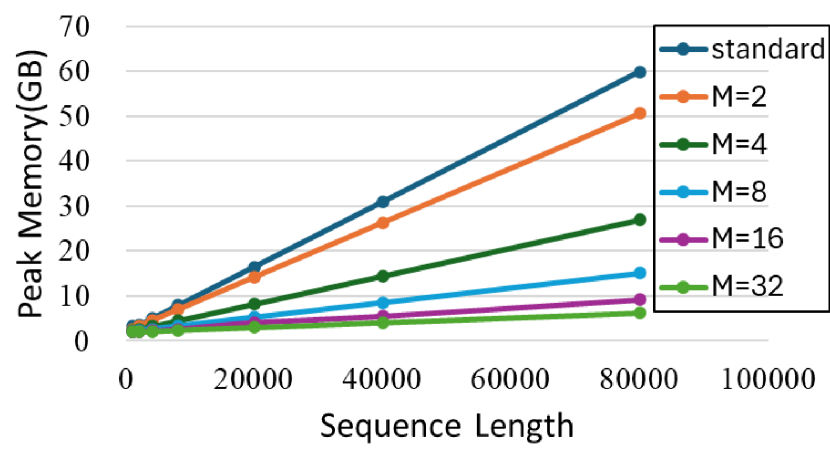
(d) Peak Memory for Llama3-8B LM-Head.

Figure 5: Time and Peak Memory for MsT’s different mini-seq setting, the experiments include both the forward and backward pass for a single layer.

6 Limitations and Future Directions

We discuss the limitations and future directions. Related work is also given in Appendix A.

Compiling to CUDA. Our current approaches are built on Pytorch implementation. This may constrain performance and low-level memory savings. It is reflected in Figure 5(c), where our implementation slows down the LM-Head performance for additional memory loading time. It can be improved by fused kernel and cuda optimization, which can be our next step. Fortunately, LM-head consumes extremely little time, and such a downgrade would not affect the overall performance.

Performance Downgrade under small sequence training. While Mini-Sequence Transformer (MsT) provides significant benefits for training transformers with extremely long sequences, it results in performance degradation when applied to models with small sequences. The overhead introduced by partitioning the input into mini-sequences and the additional memory movement required for gradient accumulation can outweigh the benefits of reduced intermediate memory usage in these scenarios. Therefore, it is important to consider the target sequence length and carefully evaluate the trade-offs before applying MsT to ensure optimal training efficiency across different sequence length scales.

Appendix A Related Work

Long Sequences Model.

The ability to train large models with long sequences is becoming increasingly crucial across various domains, from generative AI to scientific discovery. In generative AI, tasks such as conversational AI, knowledge-rich long document summarization, and video generation demand reasoning over extended contexts in both spatial and temporal dimensions. Multimodal foundation models process speech, images, and waveforms simultaneously, requiring long context reasoning over high-dimensional inputs with lengthy sequences. Similarly, chapter and book-level summarization, estimated to involve tens to hundreds of thousands of words, hold great importance in conversational AI and abstractive summarization tasks [5, 25, 32] and have demonstrated benefits from long sequence training [54, 42, 33].

The emergence of ChatGPT and subsequent open-source and commercial large language models has propelled chat applications to the forefront of modern AI, making them more relevant than ever. Efficiently processing long sequences is vital for supporting more extensive conversation histories in these applications [51]. Long sequence capability is equally critical for AI in scientific fields, enabling better understanding and advancements in healthcare [30], climate and weather forecasting [34], and large-scale molecular simulations [58].

Lossy Long Sequence Training.

One direction is making LLM able to process arbitrarily long sequences efficiently by sacrificing the perception window of the network. Sliding window attention is introduced [11] to handle infinitely long sequences as input. However, it disregards information beyond the effective receptive field. Longformer [5] extends this idea, which caches on a block-by-block basis, which increases the perception window size, so as TransformerFAM [18]. StreamLLM [53] is not constrained by a given window but selectively disregards information between the first token and given windows. They struggle to capture long-range dependencies beyond this fixed range, but the approximation quality also seems to degrade at long sequence lengths. MsT can work directly with them to increase the window size for better quality.

Memory Efficient Training.

As the demand for long sequence processing continues to grow across various domains, developing efficient methods for training large models with extended context becomes increasingly essential for advancing the state of the art in AI. Parameter-efficient fine-tuning (PEFT) methods aim to reduce the memory footprint and computational related to parameters and gradients. Adafactor [46] achieves sub-linear memory cost by factorizing the second-order statistics using a row-column outer product. Low-Rank Adaptation (LoRA) [17] reduces the memory footprint of pre-trained models using low-rank adaptors with a low-rank weight adaptor for each layer. Several variants of LoRA have been proposed to enhance its performance. [47, 56]. Quantization is another widely used technique in PEFT to reduce the memory cost of optimizer states [15].

Other techniques focus on reducing the memory footprint and computational related to activation. Gradient accumulation is a method that allows for training larger batch sizes by accumulating gradients over multiple mini-batches before performing an optimization step [35]. This approach enables training with larger effective batch sizes while maintaining a smaller physical batch size, reducing activation memory requirements. A similar work of activation offloading [40] moves the checkpointed activations to the CPU asynchronously and prefetches the offloaded activations back from the CPU during backward. There are related works in sparse Transformers, mainly focusing on full-attention approximation, such as sparse attention [9, 55]. Recent works have also focused on single-GPU memory and compute-efficient attention. A popular example in this category is Flash attention [13], which leverages known techniques such as tiling and recomputation for computing and memory efficiency. These works are orthogonal to our work and can be leveraged accordingly to improve the efficiency of Transformer-based models further.

Distributed Training.

Training in a distributed way can split LLM workloads into multiple GPUs; therefore, each GPU’s memory overhead can be reduced. It includes data parallelism [24, 26, 27], tensor parallelism [48], FSDP [57] and sequence parallelism [23, 19, 28, 29].

Appendix B Algorithm Details

We describe the full details of Mini-Sequence Transformer (MsT) backward pass. Algorithm 3 shows the MLP backward, and Algorithm 4 shows the LM-Head backward.

Algorithm 3 Mini-Sequence MLP Backward

0:  Gradients of output $\nabla O\in\mathbb{R}^{N\times d}$, Matrices $X\in\mathbb{R}^{N\times d}$, Activations $I\in\mathbb{R}^{N\times I}$, Weights $W_{gate},W_{up}\in\mathbb{R}^{d\times I}$, $W_{down}\in\mathbb{R}^{I\times d}$

1:  Partition matrices $\nabla O$ into $M$ blocks $\nabla O_{1},\ldots,\nabla O_{m}$ of size $N_{m}\times d$, where $N_{m}=N/M$

2:  for $1\leq i\leq M$ do

3:     Compute $\nabla I_{i}=\nabla O_{i}W_{down}^{T}$, $\nabla I_{i}\in\mathbb{R}^{N_{m}\times I}$

4:     Compute $\nabla W_{down}+=I_{i}^{T}\nabla O_{i}$

5:     Compute $\nabla I^{\prime}_{i}=\nabla I_{i}\odot\delta(I_{i})$, where $\delta$ is the activation function derivative of SiLU

6:     Compute $\nabla X^{\prime}i=\nabla I^{\prime}iW_{up}^{T}$, $\nabla X^{\prime\prime}_{i}=\nabla I^{\prime}_{i}W_{gate}^{T}$, $\nabla X^{\prime}_{i},\nabla X^{\prime\prime}_{i}\in\mathbb{R}^{N_{m}\times d}$

7:     Compute $\nabla W_{up}+=X_{i}^{T}\nabla I^{\prime}_{i}$, $\nabla W_{gate}+=X_{i}^{T}\nabla I^{\prime}i$

8:     Compute $\nabla X_{i}=\nabla X^{\prime}_{i}+\nabla X^{\prime\prime}_{i}$, $\nabla X_{i}\in\mathbb{R}^{N_{m}\times d}$

9:  end for

10:  Concatenate $\nabla X={\nabla X_{1},\ldots,\nabla X_{m}}\in\mathbb{R}^{N\times d}$

11:  Return $\nabla X$, $\nabla W_{gate}$, $\nabla W_{up}$, $\nabla W_{down}$.

Algorithm 4 Mini-Sequence LM-Head Backward

0:  Loss gradients $\nabla loss\in\mathbb{R}^{1}$, Logits $\in\mathbb{R}^{N\times V}$, Labels $L\in\mathbb{R}^{N}$, Weights $W_{out}\in\mathbb{R}^{d\times V}$

1:  Partition labels $L$ into $M$ sub-labels $L_{1},\ldots,L_{m}$ of size $\frac{N}{m}$, where $\frac{N}{m}=\frac{N}{M}$

2:  Each mini-sequence forward

3:  for $1\leq i\leq M$ do

4:     Compute $\nabla logits_{i}=\text{CrossEntropyLossBackward}(Logits_{i},L_{i})$

5:     Delete $logits_{i}$

6:     Compute $\nabla X_{i}=\nabla logits_{i}W_{out}^{T}$, $\nabla X_{i}\in\mathbb{R}^{\frac{N}{m}\times d}$

7:     Compute $\nabla W_{out}+=X_{i}^{T}\nabla logits_{i}$

8:  end for

9:  Each mini-sequence backward

10:  for $1\leq i\leq M$ do

11:     Compute $\nabla X_{i}=\nabla X_{i}\odot\nabla loss$

12:     Compute $\nabla W_{out}=\nabla W_{out}\odot\nabla loss$

13:  end for

14:  Concatenate $\nabla X={\nabla X_{1},\ldots,\nabla X_{m}}\in\mathbb{R}^{N\times d}$

15:  Return $\nabla X$, $\nabla W_{out}$.

We now observe about MsT backward pass that when computing the gradients of MLP and LM-Head, we do not need to use full input and intermediates data. Instead, we can use $1/M$ reduced data with mini-sequence, significantly reducing the intermediate value memory overhead.

Appendix C Llama2 and Llama3: Model Architecture Comparison

This appendix highlights the key architectural differences between the Llama2-7B and Llama3-8B models implemented by Hugging Face. The main distinction lies in the configuration of the MLP blocks and LM-Head (linear with cross-entropy loss) within the model architecture.

Figure 6: Standard Transformer architecture with the highlight of LM-head and MLP.

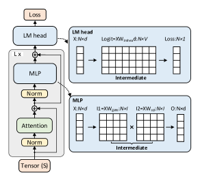
Figure 6 illustrates a standard Transformer model’s architecture, focusing on the MLP and LM-head components. The intermediate tensors (I1, I2) have larger dimensions than the input and output. Also, the logit tensor has a much larger vocabulary dimension (V) than the hidden dimension (d).

Llama2-7B Model Architecture:

Figure 7: Model Architecture of HuggingFace Implementation of Llama2-7B.

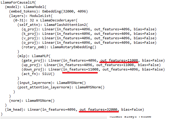
As shown in Figure 7, the Llama2-7B model employs an MLP block configuration with the following characteristics:

• MLP Block: The first linear layer projects the input from a hidden size of 4096 to an intermediate size of 11008. The second linear layer projects the intermediate representation from 11008 to 4096, the hidden size.

• LM-Head (Output Projection with Linear Loss): The LM-Head in Llama2-7B consists of a linear layer that projects the hidden representation from a size of 4096 to a vocabulary size of 32000. The output of the linear layer is then passed through a cross-entropy loss function to compute the training loss.

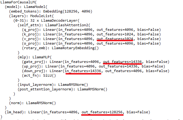
Llama3-8B Model Architecture:

Figure 8: Model Architecture of HuggingFace Implementation of Llama3-8B.

• MLP Block: The first linear layer projects the input from a hidden size of 5120 to a larger intermediate size of 13824. The second linear layer then projects the intermediate representation from a size of 13824 back to the hidden size of 5120.

• LM-Head (Linear with Cross-Entropy Loss): In Llama3-8B, the LM-Head also consists of a linear layer, but it projects the hidden representation from a size of 5120 to a larger vocabulary size of 32000. Like Llama2-7B, the output of the linear layer is passed through a cross-entropy loss function to compute the training loss.

The increased intermediate size in the MLP block of Llama3-8B allows the model to capture complex patterns and transformations more effectively. Additionally, the larger vocabulary size in the LM-HEAD of Llama3-8B enables the model to generate more diverse and nuanced outputs.

It is worth noting that while the dimensions of the MLP block and LM-Head differ between Llama2-7B and Llama3-8B, the overall structure and functionality of these components remain the same. The cross-entropy loss function in the LM-Head measures the discrepancy between the predicted word probabilities and the target words during training, guiding the model to generate more accurate and contextually relevant outputs. These architectural differences contribute to Llama3-8B’s enhanced performance and capabilities compared to its predecessor, Llama2-7B, while maintaining a consistent overall structure. However, the unexpected large intermediate value also comes from the change of MLP blocks and LM-HEAD (linear with cross-entropy loss), which we will discuss in the following section.

Moreover, this trend is also reflected in the Microsoft development of Phi-3 [2] compared with Phi-2 [20]. Whose vocabulary size increased from 50k to 100K ($2\times$), intermediate size increased from 10k to 16k ($1.6\times$), and hidden size slightly increased from 2560 to 3072 ($1.2\times$).

In conclusion, these models share an obvious trend: the ratio between intermediate and hidden size (also vocabulary and hidden size) is becoming larger.

Figure 9: Memory Visualizaion of training Llama3 8B with 4k sequence length on A100-80G.

Appendix D Mini-Sequence Transformer’s Memory Optimization Detials

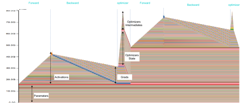
We compare Mini-Sequence Transformer (MsT) with capturing and visualizing memory snapshots. We take vanilla Pytorch training for Llama3-8B with 4k sequence length as an example to show how the memory changes with the timeline.

vanilla.

Figure 9 shows the vanilla example. The model parameters had already been loaded into memory before the training step, so we immediately see a chunk of memory devoted to the weights. For Llama3-8B, its weight would be 15GB. As we start our forward pass, memory is allocated gradually for the activations or the tensors we are saving to be able to compute gradients in the backward pass. Here, the memory allocated for activation is larger than the weight, with around 29GB. Once we start the backward pass, the activations are gradually freed while the memory of the gradients starts building up. As the gradient is equal to the size of weights, which is smaller than activation, we can observe the memory usage drop to around 30 GB. Lastly, as the optimizer kicks in, its state will be lazily initialized, so we should see the optimizer state memory gradually increase during the optimizer step of the first training loop only. In future loops, the optimizer memory will remain and be updated. The memory for the gradients is then freed accordingly at the end of every training loop when it is called zero grade. Here, the optimizer would take $2\times$ of weights when using Adam with 30GB, and the optimizer intermediate is equal to the size of weight with 15. Therefore, the peak memory usage is during the optimizer step, which equals the sum size of weight, gradient, optimizer state, and optimizer intermediates, which roughly equals to $5\times$ of weight size with 75GB as shown in Table 7.

Table 7: Memory overhead of training Llama3-8B on single A100 80G GPU.

Llama3-8B-hf	Memory Overhead	Within Peak Memory
Activation	29	0
Weight	15	15
Gradient	15	15
Optimizer	45	45
Total	-	75

Figure 10: Memory Visualizaion of training Llama3 8B with 4k sequence length on A100-80G. The optimizer in the Backward technique is deployed here

optimizer-in-backward.

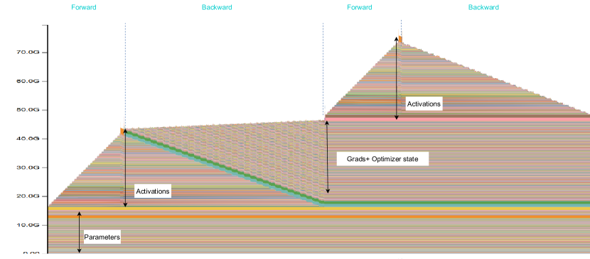
The first memory optimization discussed here is optimizer-in-backward. It fuses the optimizer state with a backward pass to save the memory of the gradient and optimizer intermediate. The memory visualization of optimizer-in-backward is shown in Figure 10, where there is no optimizer stage but only forward and backward state. The backward time would become larger as a result of fusion. Using this technology, the peak memory would change into the sum of weight, optimizer state, and activations. Although we successfully saved 30GB of memory overhead of gradient and optimizer intermediates, it adds up to 29GB memory overhead of activations, with only 1GB of memory saving. Totally it consumes 74GB of memory, as shown in Table 8. It would be worse if sequence length were increased, introducing more activation into LLM training. Therefore, optimizer-in-backward can hardly benefit long sequence training, but it simplifies the training process, so we would include this technique in the following discussion.

Table 8: Memory overhead of training Llama3-8B on single A100 80G GPU. The optimizer in the Backward technique is deployed.

Llama3-8B-hf	Memory Overhead	Within Peak Memory
Activation	29	29
Weight	15	15
Gradient	15	0
Optimizer	30	30
Total	-	74

Figure 11: Memory Visualizaion of training Llama3 8B with 4k sequence length on A100-80G. Activation Recomputation technique is deployed here

Activation Recomputation.

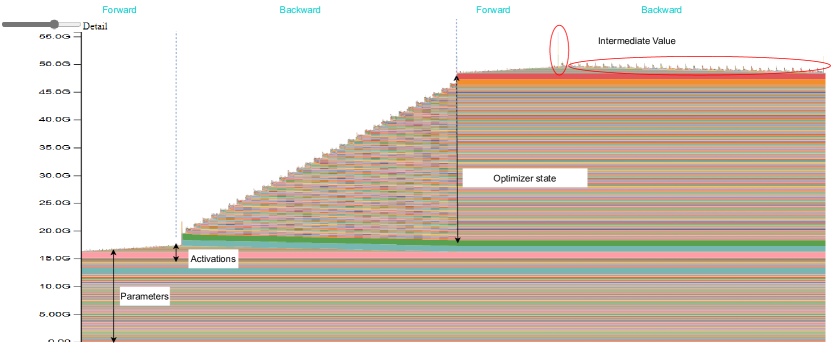
Activation Recomputation is a powerful technique used in our analysis. It can significantly reduce the activation at the cost of a small decrease in the training speed due to recomputing parts of the graph during back-propagation. As shown in figure 11, it successfully reduces the total memory overhead from 74GB to 52GB and reduces activation memory overhead from 29GB to 7GB with $4\times$ memory saving. However, we can easily find many singular points in the graph, which appear as an impulse signal. This impulse signal’s duration is concise, meaning that it is intermediate data that is briefly created in the forward/backward pass and immediately removed from the GPU HBM memory. The most prominent intermediate data is several times the total activation (4-5 times in our data analysis). These intermediate data seriously affect the training performance of long sequences and become the activation bottleneck of the row.

Table 9: Memory overhead of training Llama3-8B on single A100 80G GPU. Activation Recomputation technique is deployed.

Llama3-8B-hf	Memory Overhead	Within Peak Memory
Activation	7	7
Weight	15	15
Gradient	15	0
Optimizer	30	30
Total	-	52

Figure 12: Memory Visualizaion of training Llama3 8B with 4k sequence length on A100-80G. Mini-Sequence Transformer technique is deployed here

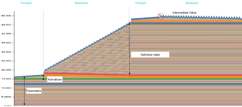
Mini-Sequence Transformer (MsT)

Inspired by the observation from Activation Recomputation techniques, we propose MsT to reduce the intermediate value during training. We successfully decrease the memory overhead of activation from 7GB to 4GB, while the intermediate value is significantly reduced. This is because only $1/M$ intermediate values are used for computing the forward outputs, backward errors, and gradients during both the forward and backward.

Table 10: Memory overhead of training Llama3-8B on single A100 80G GPU. Mini-Sequence Transformer technique is deployed.

Llama3-8B-hf	Memory Overhead	Within Peak Memory
Activation	4	4
Weight	15	15
Gradient	15	0
Optimizer	30	30
Total	-	49

Figure 13: Memory Visualization. (a) The memory timeline of training Llama3-8B using standard transformer architecture, Red cycle highlights the intermediate memory (b) The memory timeline of training Llama3-8B using MsT, Red cycle highlights the intermediate memory has been narrowed.

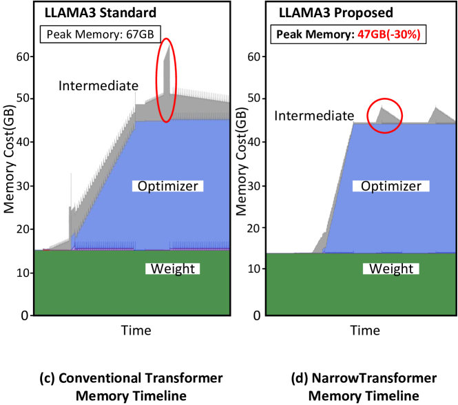
In conclusion, we compare the memory usage over time when training the Llama3-8B model using the standard transformer architecture versus using MsT, which is shown on 13.

In Figure 13(a), which shows the memory timeline for the standard Llama3-8B training, we can see that the memory usage is dominated by three main components: the model weights (in blue), the optimizer state (in green), and the intermediate memory (highlighted by the red circle). The peak memory usage reaches around 67GB.

In contrast, Figure 13(b) demonstrates the memory timeline when training Llama3-8B with MsT. The critical difference is that the intermediate memory, again highlighted by the red circle, has been significantly reduced or "narrowed" compared to the standard transformer case. As a result, the peak memory usage with MsT is around 47GB, achieving a $30\%$ reduction compared to the standard transformer.

The memory timelines illustrate that MsT effectively reduces the intermediate memory footprint during training, significantly contributing to overall memory consumption. By minimizing the intermediate memory, MsT enables more efficient memory utilization and allows training with longer sequence lengths or larger batch sizes while staying within the hardware’s available memory limits.

Appendix E Scaling to Extreme Long Sequence on Distributed Setting

We evaluate our distributed extension of MsT on Llama2-7B models and compare against vanilla DeepSpeed-Ulysses‘s sequence parallelism on 2,4,8 GPUs, respectively, for the max sequence length and corresponding training time. The results of this evaluation are shown in Table 11. Note that a distributed setting would introduce additional memory overhead, which affects the memory effect.

Table 11: Maximum sequence length of Llama3-8B, running on single A100 80G GPU.

Model Implementation	GPU numbers
	2	4	8
Llama2-7B-hf activation recomputation	24	48	96
Llama2-7B-hf MsT	32	64	128

Appendix F How many mini-sequences are needed during pre-training

Here, we provide detailed data for plotting Figure 5. We also provide insights into the performance characteristics and memory usage of the Llama3-8B model when using the Mini-Sequence Transformer (MsT) approach with different numbers of mini-sequences (M) and sequence lengths.

Table 12 shows the execution time for different sequence lengths and mini-sequence settings. As the number of mini-sequences (M) increases, the execution time slightly increases, especially for shorter sequences. However, for longer sequences (e.g., 80000), the execution time remains relatively stable across different mini-sequences (M).

Table 12: LM-head time for different sequence lengths and mini-sequence settings

LM-head time	1024	2048	4096	8192	20000	40000	80000
standard	0.01	0.02	0.04	0.09	0.2	0.4	0.85
M=2	0.02	0.04	0.07	0.14	0.31	0.67	1.36
M=4	0.03	0.04	0.07	0.14	0.33	0.67	1.33
M=8	0.04	0.05	0.08	0.14	0.34	0.67	1.34
M=16	0.06	0.07	0.09	0.16	0.34	0.68	1.35
M=32	0.11	0.11	0.14	0.19	0.37	0.69	1.36

Table 13 shows the memory usage in gigabytes (GB) for different sequence lengths and mini-sequence settings for the LM-Head component. The standard setting without mini-sequences consumes 59.92 GB for a sequence length of 80000. By increasing the number of mini-sequences, memory usage decreases significantly. With M=16, the memory usage reduces to 9.12 GB for the same sequence length, achieving an 84.8% reduction in memory consumption. This is further improved with M=32 to 89.8%.

Table 13: LM-head memory usage (in GB) for different sequence lengths and mini-sequence settings

LM-head memory	1024	2048	4096	8192	20000	40000	80000
standard	3.20	3.46	4.94	7.91	16.46	30.95	59.92
mini-seq=2	2.59	3.21	4.46	6.95	14.14	26.31	50.66
mini-seq=4	2.28	2.60	3.24	4.52	8.20	14.44	26.92
mini-seq=8	2.13	2.30	2.63	3.30	5.24	8.51	15.05
mini-seq=16	2.06	2.15	2.33	2.70	4.14	5.54	9.12
mini-seq=32	2.02	2.07	2.18	2.39	3.01	4.06	6.15

Table 14 shows the execution time for different sequence lengths and mini-sequence settings. Like the LM-Head, increasing M leads to slightly longer execution times, particularly for shorter sequences. However, the impact on execution time is minimal for longer sequences (e.g., 80000).

Table 14: MLP time (in seconds) for different sequence lengths and mini-sequence settings

MLP time	1024	2048	4096	8192	20000	40000	80000
standard	0.05	0.08	0.16	0.31	0.74	1.52	2.96
M=2	0.05	0.10	0.17	0.32	0.76	1.49	3.05
M=4	0.07	0.11	0.19	0.33	0.79	1.52	2.99
M=8	0.12	0.15	0.22	0.38	0.81	1.58	3.05

For the MLP component, Table 15 demonstrates the memory usage for different sequence lengths and mini-sequence settings. The standard setting consumes 14.72 GB for a sequence length of 80000, while using M=8 mini-sequences reduces the memory usage to 11.66 GB, resulting in a 20.8% reduction. Here, we can observe.

Table 15: MLP memory usage (in GB) for different sequence lengths and mini-sequence settings

MLP memory	1024	2048	4096	8192	20000	40000	80000
standard	0.93	1.09	1.39	2.11	4.18	7.69	14.72
M=2	1.29	1.36	1.50	2.00	3.76	6.73	12.69
M=4	1.32	1.41	1.61	2.00	3.49	6.21	11.66
M=8	1.33	1.44	1.66	2.11	3.42	6.17	11.66

The analysis suggests that increasing the number of mini-sequences (M) can significantly reduce memory usage, especially for the LM-Head component, while having a minimal impact on execution time for longer sequences. Memory savings are more pronounced for the LM-Head than for the MLP.

It is important to note that while MsT is highly beneficial for training with extremely long sequences, it may lead to performance degradation when applied to models with shorter sequences due to the overhead introduced by partitioning the input and the additional memory movement required for gradient accumulation. It can be easily observed from Table 12 that using M=32 mini-sequences increases the execution time from 0.01s (standard setting) to 0.11s for a sequence length of 1024, causing an 11x performance downgrade. Also, from Table 14, using M=8 mini-sequences increases the execution time from 0.05s (standard setting) to 0.12s for a sequence length of 1024, causing a 2x performance downgrade. The performance reduction is more pronounced for the LM-Head compared to the MLP. Fortunately, LM-head accounts for very little of the transformer’s running time, which is smaller than MLP and much smaller than attention, so our technology will not affect the overall performance, even if it affects its module performance.

References

- [1] Transformer in triton. https://github.com/lucidrains/triton-transformer.
- [2] Marah Abdin, Sam Ade Jacobs, Ammar Ahmad Awan, Jyoti Aneja, Ahmed Awadallah, Hany Awadalla, Nguyen Bach, Amit Bahree, Arash Bakhtiari, Harkirat Behl, et al. Phi-3 technical report: A highly capable language model locally on your phone. arXiv preprint arXiv:2404.14219, 2024.
- [3] Joshua Ainslie, James Lee-Thorp, Michiel de Jong, Yury Zemlyanskiy, Federico Lebrón, and Sumit Sanghai. Gqa: Training generalized multi-query transformer models from multi-head checkpoints. arXiv preprint arXiv:2305.13245, 2023.
- [4] Dzmitry Bahdanau, Kyunghyun Cho, and Yoshua Bengio. Neural machine translation by jointly learning to align and translate. arXiv preprint arXiv:1409.0473, 2014.
- [5] Iz Beltagy, Matthew E Peters, and Arman Cohan. Longformer: The long-document transformer. arXiv preprint arXiv:2004.05150, 2020.
- [6] Tianqi Chen, Bing Xu, Chiyuan Zhang, and Carlos Guestrin. Training deep nets with sublinear memory cost. arXiv preprint arXiv:1604.06174, 2016.
- [7] Yukang Chen, Shengju Qian, Haotian Tang, Xin Lai, Zhijian Liu, Song Han, and Jiaya Jia. Longlora: Efficient fine-tuning of long-context large language models. arXiv preprint arXiv:2309.12307, 2023.
- [8] Zonglei Chen, Minbo Ma, Tianrui Li, Hongjun Wang, and Chongshou Li. Long sequence time-series forecasting with deep learning: A survey. Information Fusion, 97:101819, 2023.
- [9] Rewon Child, Scott Gray, Alec Radford, and Ilya Sutskever. Generating long sequences with sparse transformers. arXiv preprint arXiv:1904.10509, 2019.
- [10] Aakanksha Chowdhery, Sharan Narang, Jacob Devlin, Maarten Bosma, Gaurav Mishra, Adam Roberts, Paul Barham, Hyung Won Chung, Charles Sutton, Sebastian Gehrmann, et al. Palm: Scaling language modeling with pathways. Journal of Machine Learning Research, 24(240):1–113, 2023.
- [11] Zihang Dai, Zhilin Yang, Yiming Yang, Jaime Carbonell, Quoc V Le, and Ruslan Salakhutdinov. Transformer-xl: Attentive language models beyond a fixed-length context. arXiv preprint arXiv:1901.02860, 2019.
- [12] Tri Dao. Flashattention-2: Faster attention with better parallelism and work partitioning. arXiv preprint arXiv:2307.08691, 2023.
- [13] Tri Dao, Dan Fu, Stefano Ermon, Atri Rudra, and Christopher Ré. Flashattention: Fast and memory-efficient exact attention with io-awareness. Advances in Neural Information Processing Systems, 35:16344–16359, 2022.
- [14] Ofer Dekel, Ran Gilad-Bachrach, Ohad Shamir, and Lin Xiao. Optimal distributed online prediction using mini-batches. Journal of Machine Learning Research, 13(1), 2012.
- [15] Tim Dettmers, Artidoro Pagnoni, Ari Holtzman, and Luke Zettlemoyer. Qlora: Efficient finetuning of quantized llms. Advances in Neural Information Processing Systems, 36, 2024.
- [16] Joeri R Hermans, Gerasimos Spanakis, and Rico Möckel. Accumulated gradient normalization. In Asian Conference on Machine Learning, pages 439–454. PMLR, 2017.
- [17] Edward J Hu, Yelong Shen, Phillip Wallis, Zeyuan Allen-Zhu, Yuanzhi Li, Shean Wang, Lu Wang, and Weizhu Chen. Lora: Low-rank adaptation of large language models. arXiv preprint arXiv:2106.09685, 2021.
- [18] Dongseong Hwang, Weiran Wang, Zhuoyuan Huo, Khe Chai Sim, and Pedro Moreno Mengibar. Transformerfam: Feedback attention is working memory. arXiv preprint arXiv:2404.09173, 2024.
- [19] Sam Ade Jacobs, Masahiro Tanaka, Chengming Zhang, Minjia Zhang, Leon Song, Samyam Rajbhandari, and Yuxiong He. Deepspeed ulysses: System optimizations for enabling training of extreme long sequence transformer models. arXiv preprint arXiv:2309.14509, 2023.
- [20] Mojan Javaheripi, Sébastien Bubeck, Marah Abdin, Jyoti Aneja, Sebastien Bubeck, Caio César Teodoro Mendes, Weizhu Chen, Allie Del Giorno, Ronen Eldan, Sivakanth Gopi, et al. Phi-2: The surprising power of small language models. Microsoft Research Blog, 2023.
- [21] Albert Q Jiang, Alexandre Sablayrolles, Arthur Mensch, Chris Bamford, Devendra Singh Chaplot, Diego de las Casas, Florian Bressand, Gianna Lengyel, Guillaume Lample, Lucile Saulnier, et al. Mistral 7b. arXiv preprint arXiv:2310.06825, 2023.
- [22] Sarit Khirirat, Hamid Reza Feyzmahdavian, and Mikael Johansson. Mini-batch gradient descent: Faster convergence under data sparsity. In 2017 IEEE 56th Annual Conference on Decision and Control (CDC), pages 2880–2887. IEEE, 2017.
- [23] Vijay Anand Korthikanti, Jared Casper, Sangkug Lym, Lawrence McAfee, Michael Andersch, Mohammad Shoeybi, and Bryan Catanzaro. Reducing activation recomputation in large transformer models. Proceedings of Machine Learning and Systems, 5, 2023.
- [24] Alex Krizhevsky, Ilya Sutskever, and Geoffrey E Hinton. Imagenet classification with deep convolutional neural networks. Communications of the ACM, 60(6):84–90, 2017.
- [25] Wojciech Kryściński, Nazneen Rajani, Divyansh Agarwal, Caiming Xiong, and Dragomir Radev. Booksum: A collection of datasets for long-form narrative summarization. arXiv preprint arXiv:2105.08209, 2021.
- [26] Mu Li, David G Andersen, Jun Woo Park, Alexander J Smola, Amr Ahmed, Vanja Josifovski, James Long, Eugene J Shekita, and Bor-Yiing Su. Scaling distributed machine learning with the parameter server. In 11th USENIX Symposium on operating systems design and implementation (OSDI 14), pages 583–598, 2014.
- [27] Mu Li, David G Andersen, Alexander J Smola, and Kai Yu. Communication efficient distributed machine learning with the parameter server. Advances in Neural Information Processing Systems, 27, 2014.
- [28] Shenggui Li, Fuzhao Xue, Chaitanya Baranwal, Yongbin Li, and Yang You. Sequence parallelism: Long sequence training from system perspective. arXiv preprint arXiv:2105.13120, 2021.
- [29] Hao Liu, Matei Zaharia, and Pieter Abbeel. Ring attention with blockwise transformers for near-infinite context. arXiv preprint arXiv:2310.01889, 2023.
- [30] Xin Liu, Daniel McDuff, Geza Kovacs, Isaac Galatzer-Levy, Jacob Sunshine, Jiening Zhan, Ming-Zher Poh, Shun Liao, Paolo Di Achille, and Shwetak Patel. Large language models are few-shot health learners. arXiv preprint arXiv:2305.15525, 2023.
- [31] Ilya Loshchilov and Frank Hutter. Decoupled weight decay regularization. arXiv preprint arXiv:1711.05101, 2017.
- [32] Lefteris Loukas, Manos Fergadiotis, Ion Androutsopoulos, and Prodromos Malakasiotis. Edgar-corpus: Billions of tokens make the world go round. arXiv preprint arXiv:2109.14394, 2021.
- [33] Meta. Introducing meta llama 3: The most capable openly available llm to date. https://ai.meta.com/blog/meta-llama-3/.
- [34] Tung Nguyen, Johannes Brandstetter, Ashish Kapoor, Jayesh K Gupta, and Aditya Grover. Climax: A foundation model for weather and climate. arXiv preprint arXiv:2301.10343, 2023.
- [35] Myle Ott, Sergey Edunov, David Grangier, and Michael Auli. Scaling neural machine translation. arXiv preprint arXiv:1806.00187, 2018.
- [36] Markus N Rabe and Charles Staats. Self-attention does not need o (n2̂) memory. arXiv preprint arXiv:2112.05682, 2021.
- [37] Alec Radford, Karthik Narasimhan, Tim Salimans, Ilya Sutskever, et al. Improving language understanding by generative pre-training. preprint, 2018.
- [38] Alec Radford, Jeffrey Wu, Rewon Child, David Luan, Dario Amodei, Ilya Sutskever, et al. Language models are unsupervised multitask learners. OpenAI blog, 1(8):9, 2019.
- [39] Colin Raffel, Noam Shazeer, Adam Roberts, Katherine Lee, Sharan Narang, Michael Matena, Yanqi Zhou, Wei Li, and Peter J Liu. Exploring the limits of transfer learning with a unified text-to-text transformer. Journal of machine learning research, 21(140):1–67, 2020.
- [40] Samyam Rajbhandari, Olatunji Ruwase, Jeff Rasley, Shaden Smith, and Yuxiong He. Zero-infinity: Breaking the gpu memory wall for extreme scale deep learning. In Proceedings of the international conference for high performance computing, networking, storage and analysis, pages 1–14, 2021.
- [41] Prajit Ramachandran, Barret Zoph, and Quoc V Le. Searching for activation functions. arXiv preprint arXiv:1710.05941, 2017.
- [42] Machel Reid, Nikolay Savinov, Denis Teplyashin, Dmitry Lepikhin, Timothy Lillicrap, Jean-baptiste Alayrac, Radu Soricut, Angeliki Lazaridou, Orhan Firat, Julian Schrittwieser, et al. Gemini 1.5: Unlocking multimodal understanding across millions of tokens of context. arXiv preprint arXiv:2403.05530, 2024.
- [43] Aurko Roy, Mohammad Saffar, Ashish Vaswani, and David Grangier. Efficient content-based sparse attention with routing transformers. Transactions of the Association for Computational Linguistics, 9:53–68, 2021.
- [44] Reuven Rubinstein. The cross-entropy method for combinatorial and continuous optimization. Methodology and computing in applied probability, 1:127–190, 1999.
- [45] Noam Shazeer. Fast transformer decoding: One write-head is all you need. arXiv preprint arXiv:1911.02150, 2019.
- [46] Noam Shazeer and Mitchell Stern. Adafactor: Adaptive learning rates with sublinear memory cost. In International Conference on Machine Learning, pages 4596–4604. PMLR, 2018.
- [47] Ying Sheng, Shiyi Cao, Dacheng Li, Coleman Hooper, Nicholas Lee, Shuo Yang, Christopher Chou, Banghua Zhu, Lianmin Zheng, Kurt Keutzer, et al. S-lora: Serving thousands of concurrent lora adapters. arXiv preprint arXiv:2311.03285, 2023.
- [48] Mohammad Shoeybi, Mostofa Patwary, Raul Puri, Patrick LeGresley, Jared Casper, and Bryan Catanzaro. Megatron-lm: Training multi-billion parameter language models using model parallelism. arXiv preprint arXiv:1909.08053, 2019.
- [49] Philippe Tillet, Hsiang-Tsung Kung, and David Cox. Triton: an intermediate language and compiler for tiled neural network computations. In Proceedings of the 3rd ACM SIGPLAN International Workshop on Machine Learning and Programming Languages, pages 10–19, 2019.
- [50] Together AI. togethercomputer/Long-Data-Collections. https://huggingface.co/datasets/togethercomputer/Long-Data-Collections.
- [51] Hugo Touvron, Louis Martin, Kevin Stone, Peter Albert, Amjad Almahairi, Yasmine Babaei, Nikolay Bashlykov, Soumya Batra, Prajjwal Bhargava, Shruti Bhosale, et al. Llama 2: Open foundation and fine-tuned chat models. arXiv preprint arXiv:2307.09288, 2023.
- [52] Ashish Vaswani, Noam Shazeer, Niki Parmar, Jakob Uszkoreit, Llion Jones, Aidan N Gomez, Łukasz Kaiser, and Illia Polosukhin. Attention is all you need. Advances in neural information processing systems, 30, 2017.
- [53] Guangxuan Xiao, Yuandong Tian, Beidi Chen, Song Han, and Mike Lewis. Efficient streaming language models with attention sinks. arXiv preprint arXiv:2309.17453, 2023.
- [54] Wenhan Xiong, Jingyu Liu, Igor Molybog, Hejia Zhang, Prajjwal Bhargava, Rui Hou, Louis Martin, Rashi Rungta, Karthik Abinav Sankararaman, Barlas Oguz, et al. Effective long-context scaling of foundation models. arXiv preprint arXiv:2309.16039, 2023.
- [55] Manzil Zaheer, Guru Guruganesh, Kumar Avinava Dubey, Joshua Ainslie, Chris Alberti, Santiago Ontanon, Philip Pham, Anirudh Ravula, Qifan Wang, Li Yang, et al. Big bird: Transformers for longer sequences. Advances in neural information processing systems, 33:17283–17297, 2020.
- [56] Jiawei Zhao, Zhenyu Zhang, Beidi Chen, Zhangyang Wang, Anima Anandkumar, and Yuandong Tian. Galore: Memory-efficient llm training by gradient low-rank projection. arXiv preprint arXiv:2403.03507, 2024.
- [57] Yanli Zhao, Andrew Gu, Rohan Varma, Liang Luo, Chien-Chin Huang, Min Xu, Less Wright, Hamid Shojanazeri, Myle Ott, Sam Shleifer, et al. Pytorch fsdp: experiences on scaling fully sharded data parallel. arXiv preprint arXiv:2304.11277, 2023.
- [58] Maxim Zvyagin, Alexander Brace, Kyle Hippe, Yuntian Deng, Bin Zhang, Cindy Orozco Bohorquez, Austin Clyde, Bharat Kale, Danilo Perez-Rivera, Heng Ma, et al. Genslms: Genome-scale language models reveal sars-cov-2 evolutionary dynamics. The International Journal of High Performance Computing Applications, 37(6):683–705, 2023.