Separable DeepONet: Breaking the Curse of Dimensionality in Physics-Informed Machine Learning
Abstract
The deep operator network (DeepONet), a popular neural operator architecture, has demonstrated significant promise in solving partial differential equations (PDEs) by leveraging deep neural networks to map between infinite-dimensional function spaces. In scenarios without labeled datasets, we utilize the PDE residual loss to learn the physical system. This approach, referred to as physics-informed DeepONet, encounters substantial computational challenges, particularly due to curse of dimensionality the computational cost grows exponentially with increasing discretization density. In this paper, we introduce the separable DeepONet (Sep-DeepONet) framework to overcome these challenges and enhance scalability for high-dimensional PDEs. Our approach presents a factorization technique, wherein sub-networks handle individual one-dimensional coordinates, thereby reducing the number of forward passes and the size of the Jacobian matrix. By employing forward-mode automatic differentiation (AD), we further optimize the computational cost associated with the Jacobian matrix. Consequently, our modifications result in a linear scaling of computational cost with discretization density, making the Sep-DeepONet highly suitable for high-dimensional PDEs. We validate the effectiveness of the separable architecture through three benchmark PDE models: the viscous Burgers equation, Biot’s consolidation theory, and a parametrized heat equation. In all cases, our proposed framework achieves comparable or improved accuracy while significantly reducing computational time compared to the conventional DeepONet. These findings demonstrate the potential of Sep-DeepONet in efficiently solving complex, high-dimensional PDEs, thereby advancing the field of physics-informed machine learning.
1 Introduction
Neural operator learning, which employs deep neural networks (DNNs) to learn mappings between infinite-dimensional function spaces, has recently gained significant attention, particularly for its applications in learning partial differential equations (PDEs). A classical solution operator learning task involves the learning of mapping across a range of scenarios, e.g., different domain geometries, input parameters, and initial and boundary conditions (IBCs) to the solution of the underlying PDE system. At the moment, there are a plethora of different neural operators, among which we can distinguish meta-architectures, e.g., deep operator networks (DeepONet)[21] and operators based on integral transforms, e.g., the Fourier neural operator (FNO) [20], wavelet neural operator (WNO) [27], the graph kernel network (GKN) [1] and the Laplace neural operator (LNO) [6], to name a few. In this work, we will concentrate on DeepONet, which comprises two DNNs, one DNN, known as the branch network, encodes the input functions at fixed sensor points, while another DNN, the trunk network, encodes the information related to the spatio-temporal coordinates of the output function. The solution operator is defined as the element-wise product of the embeddings of the branch network (coefficients) and the trunk network (basis functions) summed over the total number of output embeddings. The design of DeepONet is inspired by the universal approximation theorem for operators proposed by Chen & Chen [7]. The generalized theorem for DeepONet [21] replaces shallow networks used for the branch and trunk net in [7] with DNNs to gain expressivity.
The typical workflow of DeepONet involves two stages: the collection of paired labeled datasets either through running multiple experiments or through solving the governing equation multiple times using the classical solution method; followed by the second stage (learning phase) where a gradient descent-based optimizer is used to find the optimal parameters of the networks. Although the efforts associated with data generation are labeled as offline costs, the computational expenses associated with generating extensive and diverse experimental or high-fidelity simulation training data constitute the most significant investment in the entire training process. An alternative to data-driven versions is the physics-informed DeepONet (PI-DeepONet), introduced in [30] and [14]. PI-DeepONet aims to constrain the solution operator by embedding the physics into the loss function of the ML model or as constraints on the optimizer. Drawing motivation from physics-informed neural networks (PINNs), we recognize that the outputs of the DeepONet are differentiable with respect to their input coordinates. Hence, one can leverage the automatic differentiation (AD) algorithm to compute the derivatives terms present in the governing PDE. In the prior efforts on PI-DeepONet, the authors have acknowledged an exceptionally high computational cost which is attributed to the computing the derivatives. Some works have focused on optimizing the computational effort in the calculating these derivatives. This includes the investigation of the zero-coordinate shift to optimize the calculation in reverse-mode AD [19], as well as the use of factorizable coordinates in PINNs to allow for forward-mode AD [8]. Following the seminal work for separable PINNs in [8], we extend this concept to separable physics-informed DeepONet (PI-Sep-DeepONet) alongside the introduction of separable DeepONet (Sep-DeepONet) themselves in this work. Conventionally, the reverse mode AD algorithm is employed to compute the derivative terms. To understand the challenges of the conventional DeepONet framework, we consider the example of a discretization of a -dimensional domain, with one-dimensional coordinates on each axis and input functions for the branch network. For each sample evaluated through the branch net, the trunk net evaluates forward passes of a single multi-layer perceptron (MLP). Furthermore, while computing the derivatives using the reverse mode AD, the Jacobian matrix has a size . The computational cost of evaluating this matrix increases exponentially with the increase in discretization density of the domain; restricting the scalability of the approach for solving high-dimensional PDEs.
The driving idea in our work is to gain efficiency by reducing the size of the Jacobian matrix, and the number of forward passes through trunk and branch networks. To that end, we propose the following modifications:
-
•
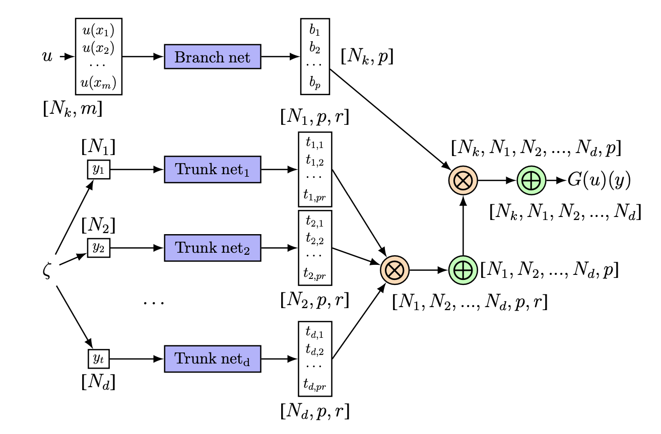
Instead of using a single MLP as the trunk network for all multidimensional coordinates, we employ factorized coordinates and separate sub-networks for each one-dimensional coordinate. Each sub-network processes its respective coordinate, and the final output is produced through an outer product and element-wise summation in the sense of a tensor rank approximation with rank . This architecture reduces the number of trunk network propagations from to .
-
•
To compute the PDE derivative terms, we use forward mode AD, significantly reducing the computational cost of the Jacobian matrix. In this separated approach, the Jacobian matrix is of size and requires evaluations with forward-mode AD, compared to the conventional evaluations with reverse mode AD.
-
•
The total number of passes through the branch network, which encodes the input function, and the trunk network, which defines the evaluation parameters, is decreased by combining all branch outputs and trunk outputs in each batch. This is done by using an outer product followed by a summation over the hidden dimension (denoted as ), effectively acting as factorized inputs over the trunk and branch network. This method further reduces the computational cost for forward passes from being proportional to to being proportional to .
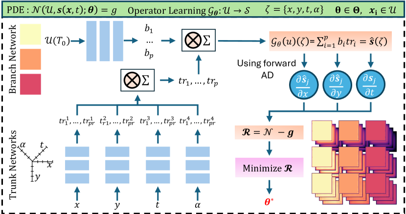
These modifications will allow the PI-Sep-DeepONet framework to scale linearly with and hence, is amenable to high-dimensional PDEs. The proposed framework for separable physics-informed DeepONet is presented in Figure 1. The network structure with batch tracing is shown in Figure S1 in the Supplementary Materials.
2 Results
To demonstrate the advantages and efficiency of the PI-Sep-DeepONet, we learn the operator for three diverse PDE models of increasing complexity and dimensionality. First, we consider the viscous Burgers equation to highlight the framework’s ability to handle nonlinearity. Our goal is to learn the solution operator that maps initial conditions to the full spatio-temporal solution of the 1D Burgers’ equation. Second, we examine a PDE describing the consolidation of a fluid-saturated body using Biot’s theory. Here, we aim to learn the solution operator that maps any loading function at the drained surface to the full spatiotemporal solution of a 1D column with a permeable top and impermeable bottom. This represents a coupled problem with two field variables. Finally, we explore the parameterized heat equation for a 2D plate. In this case, we learn the solution operator for the temporal evolution of the temperature field given an initial temperature field and thermal diffusivity. In all three examples, we obtain the results without using any labeled training data.
| Problem | Model | Relative error | Run-time (ms/iter.) |
|---|---|---|---|
| Burgers () | Vanilla | 136.6 | |
| Separable | 3.64 | ||
| Consolidation () | Vanilla | 169.43 | |
| Separable | 3.68 | ||
| Parameterized heat () | Vanilla | - | 10,416.7 |
| Separable | 91.73 |
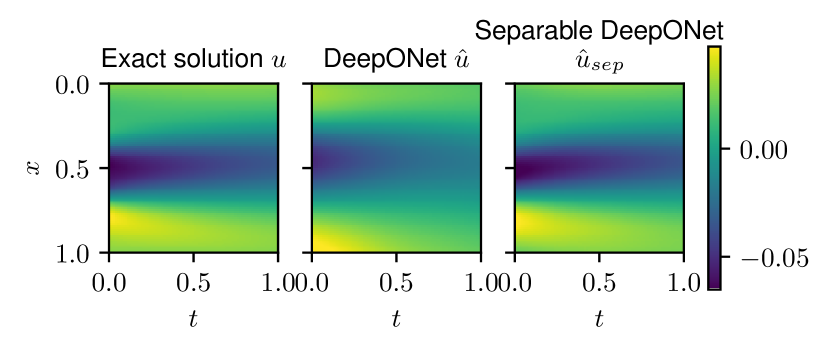
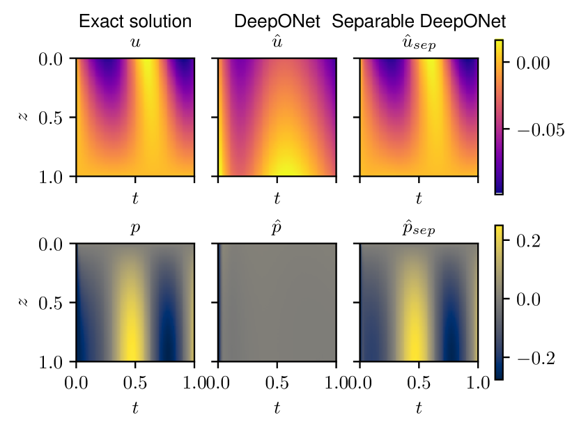
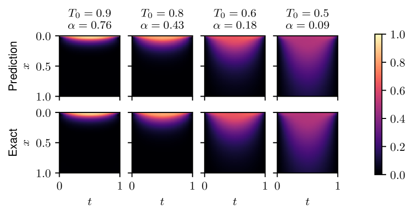
Figure 2 illustrates the performance of the proposed PI-Sep-DeepONet in comparison to vanilla PI-DeepONet after a fixed training period, for all the examples. Figure 2(a), presents the results for the Burgers example using networks with approximately 130,000 trainable parameters for both types. Meanwhile, Figure 2(b), displays the comparison for consolidation based on Biot’s theory, with 141,802 parameters for vanilla architecture and 170,022 parameters for separable architecture. Furthermore, the application of PI-Sep-DeepONet to the parameterized heat equation in two spatial dimensions, shown in Figure 2(c), showcases the enhanced performance of this approach. The separable architecture was simulated for 2.5 hours, while the vanilla architecture approximated a completion time of 2110 hours. All computations were performed on an NVIDIA A40 graphics processing unit (GPU) architecture. The code was written in Python around the packages JAX [5] and Flax [15] as well as the Deepmind Ecosystem [10].
2.1 Burgers’ equation
To provide an introductory example, we consider the viscous Burgers equation, which was also used in [30] as a benchmark example to introduce idea of PI-DeepONet, among others. The PDE reads as:
| (1) |
where and denote spatiotemporal coordinates, is the kinematic viscosity, and is the fluid velocity. The periodic boundary conditions and the initial conditions are written as:
| (2) | ||||
| (3) | ||||
| (4) |
where the initial condition is generated from a Gaussian random process. Our goal is to learn the nonlinear solution operator, that maps initial condition, to the full spatio-temporal solution, of the 1D Burgers’ equation. The code provided in [30] for PI-DeepONet was used as a benchmark. Additionally, the script provided in [30] was used to generate the numerical reference solution. We sampled 2,000 initial conditions from a Gaussian process with spectral density , where , , and , with being periodic on . Using the inverse Fourier transform, the kernel is expressed as . The spectral discretization was evaluated with 2,048 Fourier modes in spectral form using the chebfun package [11].
Half of the sampled initial conditions () were used for training, while the other half were reserved for testing. Note that only the initial conditions were used in the training process, without utilizing the generated labeled dataset of the solution. The initial condition were discretized uniformly at points and considered as inputs to the branch network evaluated at sensors. Boundary conditions were evaluated at locations, with 100 equidistant points on each side, i.e., at and . The PDE solution was evaluated at coordinate pairs of defined on a uniform lattice grid.
Training was conducted over 50,000 epochs using the Adam optimizer [17], with a batch size of 100,000. The loss function is defined as the sum of the PDE residual loss, the boundary condition loss, and the initial condition loss, where the initial condition loss is weighted with factor compared to boundary condition loss and PDE residual loss. The initial learning rate was set to and decayed exponentially at a rate of 0.95 every 1,000 epochs. Both the branch and trunk networks were designed as 7-layer networks (6 hidden layers and one output layer) with tanh activation functions and 100 neurons per layer, resulting in a hidden dimension of for the vanilla DeepONet, including the output bias term. This configuration amounted to 131,701 parameters. For the Sep-DeepONet, the governing PDE was sampled using 50 random values of and , independently, forming the basis for 2,500 factorized pairs, similar to the vanilla DeepONet. We compared three instances of Sep-DeepONet, all with identical hidden layer structures in both the trunk and branch networks, consisting of 6 hidden layers with 100 neurons each. We evaluated two different ranks and hidden sizes, and . Given that there are two separate networks in the trunk and each output layer has neurons, this configuration amounted to 244,921 and 672,151 parameters, respectively. Additionally, we considered a version with 6 hidden layers of 50 neurons and .
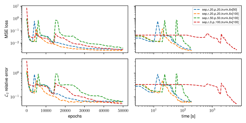
The final relative error achieved on the test data for the PI-Sep-DeepONet, the training time, and comparison to the vanilla PI-DeepONet are presented in Table 2. All models achieved comparable test results, with slightly lower test errors for the separable architecture. However, the training time and computational cost were significantly reduced for the separable architecture. The Sep-DeepONet with same parameterization as its vanilla counterpart required roughly 2.5% of the reference runtime (see Table 2). Here, reference runtime refers to the computational time requires by vanilla DeepONet to get to a similar accuracy. Figure 3 shows the loss and error curves for all variants over epochs and time, while Figure 4 compares the results on a test example for separable and vanilla DeepONet with comparable parameter counts. As seen from the loss and error curves, further improvements could be made by adjusting the learning rate settings to smoothen the curves. Some inconsistency between parameters and runtime for the Sep-DeepONet (182 s runtime for 672,151 parameters compared to roughly 197 s for 244,921 and 129,221 parameters) suggests that further improvement could be achieved through better data handling on the GPU.
| Branch | Trunk | Parameters | rel. err. | Runtime [s] | Runtime improv. | ||
|---|---|---|---|---|---|---|---|
| 6[100] | 6[100] | 100 | - | 131,701 | 6,829.2 | - | |
| 6[100] | 6[100] | 50 | 50 | 672,151 | 182.1 | -97,33% | |
| 6[100] | 6[100] | 20 | 20 | 244,921 | 197.8 | -97,10% | |
| 6[100] | 6[50] | 20 | 20 | 129,221 | 197.0 | -97,12% |
During experiments with different architecture settings, we observed that the Sep-DeepONet tends to be more prone to finding trivial solutions, such as zero solutions that satisfy the PDE and symmetry boundary conditions, compared to the classical DeepONet. Some of this behavior was mitigated by adjusting the learning rate scheduling. Nonetheless, this tendency is evident in the loss and error plots (see Figure 3).
2.2 Consolidation using Biot’s theory
The consolidation of a fluid-saturated solid body may be described using Biot’s theory [4]. This theory elucidates the interaction between solid and fluid under load, portraying a quasi-static yet transient process that provides insights into displacement and fluid or pore pressure . Biot’s theory describes a heuristic approximation, but is not based on balance equations and the associated thermodynamically consistent derivation [3]. Nevertheless, we can use these simplified equations for a study as a coupled problem as a guide to later applications. More sophisticated equations of this type can be used effectively to model advection-diffusion transport in porous media [24] as well active biological tissue [26]). Specifically, a one-dimensional column with a permeable top and impermeable bottom, subjected to a general load at the drained surface, can be mathematically represented by the PDE as:
| (5) | ||||
| (6) |
where and are the Lamé constants, and are the spatiotemporal dimensions, is Darcy’s permeability, is fluid density, and is acceleration due to gravitation. All parameters are set to . The initial and boundary conditions are as follows:
| (7) | ||||
| (8) | ||||
| (9) | ||||
| (10) | ||||
| (11) | ||||
| (12) |
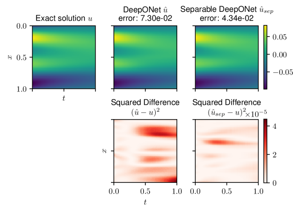
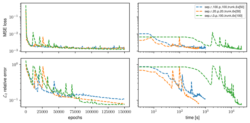
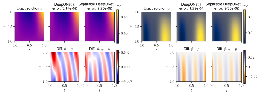
with a general load function that is sampled using a Gaussian process and the column length is denotes with . The derivation of those equations, the underlying assumptions, and the procedure to obtain an analytical solution is given in [25]. To facilitate the construction of the problem, we modify the boundary condition in equation 9 as to obtain a Dirichlet boundary condition for the displacement field. Note that this does not introduce any additional information into the system, but merely simplifies the analysis and the use of the reference solution. The load function can be taken as input from the calculated system response similar to the initial condition for pore pressure in equation 8 but does not change the underlying problem. In this problem, we aim to learn the non-linear solution operator that maps the loading function to the displacement field and the pressure field. This coupled problem has two output fields, namely displacement and pressure, which can be achieved either by defining two independent DeepONet frameworks or by splitting the last layer of the branch and the trunk networks into two groups and writing out the solution operator for each of the output [22, 13]. A preliminary examination indicated superior performance with the trunk splitting framework. The neural network was trained for 150,000 epochs using the Adam optimizer [17], employing an exponential learning rate decay starting at with a decay rate of 0.8 every 10,000 epochs. We sampled 2,000 load functions from a Gaussian process with a radial basis function kernel , with half () used for training and the rest for testing. The displacement field and the pressure were computed using the analytical step-wise solution from [25], and those corresponding to the boundary condition and initial condition were employed during the training process. For modeling the physical system, we have used 101 equidistant points for both top and bottom boundaries, as well as for the initial condition, along with 101 fixed sensors on the top boundary to monitor the arying load function. The reference network (vanilla framework) comprised 6 hidden layers of 100 neurons in the trunks and branch, with a last layer dimension of split into 2 outputs, totaling 141,802 parameters. This was compared against two Sep-DeepONet architectures with identical branch network (6 hidden layers of 100 neurons), but with only 50 neurons in each of the 6 hidden trunk layers. One network had tensor rank and hidden dimension set to , totaling 170,022 parameters, while the other had , totaling 2,136,502 parameters. Figure 5 presents the training loss and error for all three networks. The separable architecture significantly outperformed the vanilla architecture in terms of computational efficiency. Despite more rugged convergence curves suggesting potential for improved learning rate scheduling, the Sep-DeepONet achieved comparable results in terms of relative error, as shown in Figure 6. Notably, discrepancies between network results and the reference solution primarily occurred near the initial condition, indicating potential for improvement through adjusted loss weighting strategies such as self-adaptive weights [18]. All the loss terms were equally weighted. The challenge of accurately approximating the pressure field, particularly evident in the early training stages (figure 2(b)), has been studied previously [23]. Strategies to balance convergence behavior among different loss terms have shown partial mitigation, and further improvement might be achievable through methods like neural tangent kernel approaches [31]. The observed alignment of main directional field components with coordinate axes supports the hypothesis that a separable coordinate approach in the trunk aids in learning such structures. However, deeper analysis is required to definitively conclude whether Sep-DeepONet outperforms standard DeepONet with identical parameters, and thus, we refrain from making such claims at this stage. Training times differed significantly, with the vanilla DeepONet requiring 25,415 seconds, while the Sep-DeepONet was trained in 552 seconds (a reduction of 97.83%) and 997 seconds (a reduction of 96.08%), respectively.
2.3 Parameterized heat equation
As a final example, let us consider a parameterized heat equation in a two-dimensional domain. The corresponding PDE reads as:
| (13) |
where denotes temperature, , , and denote the spatiotemporal coordinates, and denotes the parameterized thermal diffusivity. We consider a two-dimensional plate with the edges set to temperature and within the domain the temperature is set to randomly chosen constant temperature. Accordingly, the initial and boundary conditions are expressed as:
| (14) | ||||
| (15) | ||||
| (16) |
where is a predefined constant temperature. The PI-Sep-DeepONet takes the initial temperature field as input to the branch network, while the spatiotemporal coordinates and thermal diffusivity are inputs to the respective trunk networks. The initial temperature is considered in the range , while the thermal diffusivity spans several magnitudes within . To incorporate this into our model, we used a parameter and squared this factor in the residual calculation.
We trained the Sep-DeepONet for 50,000 epochs using the Adam optimizer [17] with an initial learning rate of and an exponential decay rate of 0.9 every 2,000 steps. During training, 25 initial temperatures were sampled uniformly from the range . The initial condition was evaluated at a grid of spatial points, while the boundary conditions at , , , and were sampled with equidistant points in the remaining spatial dimension and time. The values of were sampled at 51 points uniformly between . Furthermore, the residual was evaluated at factorized coordinates with a uniform spacing of 31 points in , , , and .
The network was evaluated using 200 test examples, where each example had a unique combination of and sampled uniformly from their respective domains. The solutions to these inputs were obtained analytically by separation of variables and Fourier series analysis [12]. The network architecture consisted of 6 hidden layers with 50 neurons each in the trunk and branch networks, with hidden dimension and tensor rank set to . This configuration resulted in a total of 576,801 parameters with 4 separable trunk networks.
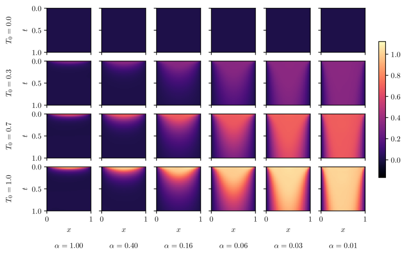
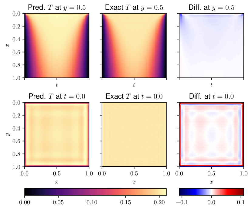
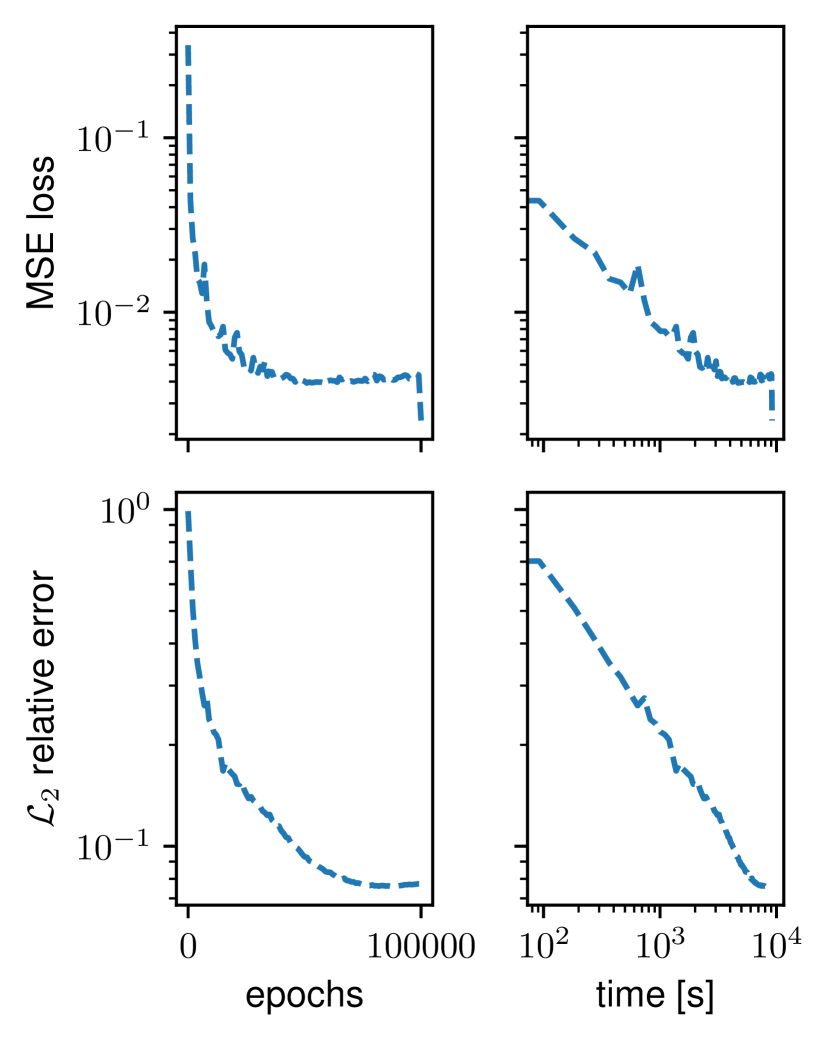
The trained network successfully solved the parameterized heat equation for the given initial temperature and thermal diffusivity throughout the domain, as shown in Figure 7. Training the Sep-DeepONet took 9173 seconds, resulting in a final relative error of over all test examples. An individual test example is depicted in Figure 8, where it is evident that the main source of error is at the outer boundary, especially for the initial condition. The prediction for this initial time step shows a spatial expression of the Gibbs phenomenon [16], caused by the jump from 0 directly at the boundary to , as well as the finite superposition of trigonometric functions for approximation. Increasing the hidden dimension and extending the training duration would likely reduce or eliminate this behavior.
In summary, we constructed a predictor on a five-dimensional domain (, , , , ) employing Sep-DeepONet and trained it for just over an hour on our in-house hardware. This demonstrates the potential of using Sep-DeepONet to significantly reduce training effort, as the dimensions can be sampled independently, thus overcoming the curse of dimensionality inherent in traditional PI-DeepONet training.
The Sep-DeepONet was trained for 100,000 epochs at a rate of 10.90 iterations per second, resulting in a total training time of approximately 2.5 hours. In contrast, a normal DeepONet required to split the training data, i.e., trunk and branch input as well as boundary and initial condition targets, into 100 batches on our GPU. This necessitated the use of mini-batches and increased the training epochs to 10,000,000, while training speed was reduced to 0.96 iterations per second, leading to a significantly extended overall training duration of approximately 2893.5 hours. With the aforementioned factor of 100, although this represents a strong reduction in complexity, a theoretical iteration time of 0.0096 iterations per second can be estimated for a full-batch. This comparison highlights the substantial impact of Sep-DeepONet on efficient training in high dimensions as Sep-DeepONet in this setup show an empirical speedup factor over 1000.
3 Discussion
Finally, we review the capabilities and limitations of physics-informed Sep-DeepONet, focusing on its efficiency and performance. A key question is whether Sep-DeepONet consistently outperforms standard DeepONet or if its main advantage is improved efficiency. Our findings suggest that while Sep-DeepONet is more computationally efficient, this does not always result in better generalization performance. The main benefit is the efficiency gained through factorizing inputs, which reduces computational cost. This efficiency can make longer training and hyperparameter tuning faster, potentially leading to better results with less computational effort. Analytical solution strategies, such as separation of variables and subsequent superposition of partial solutions (as in the heat equation), indicate that calculating solutions as a function of the trunk inputs forms the basis of the solution methodology. Thus, it can be assumed for such examples that the method of calculation via independent trunk networks and subsequent combination by outer products and summation is closer to the analytical solution strategy than the calculation in only one network for trunk and branch each.
It is also important to note that only a subset of DeepONet architectures were evaluated in this study. We primarily focused on unstacked DeepONet. However, there are indications that both stacked and unstacked configurations can be effective in their respective settings regarding performance and generalization capabilities [21, 22]. Along with the strategy for handling multiple outputs, this opens up exciting potential for further exploration and optimization. Although only classical feed-forward neural networks were used in this study, the concept is directly applicable to other architectures such as convolution or recurrent neural networks, as well as architectures with residual connections [29]. Similarly, for PI-Sep-DeepONet, all changes to the physics-informed part can be modified in the same way as for standard PI-DeepONet, similar to PINNs. This includes causality-respecting [28] or variational formulations of the loss [14], as well as hard constraint boundary conditions [22].
Despite the theoretical advantages, practical implementation has shown that Sep-DeepONet do not achieve the expected speedup. This discrepancy may be attributed to issues related to data handling on the GPU. This will be handled in our future work. Efficient handling of the data on the GPU and thus addressing this issue is critical for fully realizing the potential of PI-Sep-DeepONet.
The Sep-DeepONet requires factorized inputs, encompassing parameters, coordinates, and load functions. This requirement can be both a strength and a limitation. On one hand, it allows the model to efficiently handle high-dimensional data. On the other hand, it imposes constraints on the types of data arrangements in the domain that can be processed without additional pre-processing steps or more elaborate setups. While PINNs and PI-DeepONet are meshless methods, the separable framework requires the solution to be defined on a grid in data handling. In particular, when using real measurement data, which may have been obtained at different points on the spatiotemporal domain and under various conditions, it cannot be included without pre-processing. In addition to using interpolation methods (as long as applicable), one remedy is that spatiotemporal locations for every sample have to be considered as inputs to the trunk network independently; the trunk network inputs will have a batch dimension beyond just the discretization on each axis. More precisely, in Figure S1, the input dimensions of the trunk network would be modified as , where denotes the number of samples and denotes the discretization in the dimensionality and . Although the separable architecture is still usable, one cannot leverage the full computational benefits. Another scenario where the computational benefits of the separable framework cannot be fully leveraged is if specific location-specific parametric values of the PDE have to be assigned. In such a case, one cannot separate the dimensions and hence has to use the trunk network from the vanilla framework.
One drawback of the separable framework is the increase in network size (output layer) driven by the tensor decomposition of rank . However, the latent dimension of the network outputs in the trunk includes the hidden dimension in the output size . This enables a resizing of the latent dimension by reducing the vanilla hidden dimension while simultaneously increasing as done in our examples. This can alleviate the problem, but network size is a relevant topic for Sep-DeepONet. Nevertheless, the number of parameters also scales with the number of trunk inputs and thus networks. In this context, though, it is also true that potentially smaller networks, as in the examples, may yield equal or better results and expressivity when compared to the vanilla architecture. Furthermore, we note that even networks with a significantly higher number of trainable parameters (because of multiple trunk networks) do not require a significant increase in computing time. This may be due to the potential for improvement in memory management and the resulting increase in computing time, which exceeds the computing time required for the vanilla network. A deeper investigation of the capacity and (empirical) approximation properties of Sep-DeepONet compared to vanilla DeepONet is desirable in this regard. Another possibility is that all these networks could be trained parallely, therrby further improving efficiency.
In addition to the potentially higher memory consumption due to larger network architectures, consideration must also be given to the memory consumption due to factorized coordinates. At this point, the curse of dimensionality comes back into the calculation, as the sampling in a grid scales with the dimension of the input data. Nonetheless, a mini-batch-based calculation can be used to create a compromise between efficiency and memory consumption. It’s important to mention that comparable sampling with vanilla DeepONet suffers more severely under the curse of dimensionality in terms of memory requirements when creating the input and ground truth for the data part. Another beneficial point is the use of random inputs, which are resampled in the domain in each iteration. This can reduce the number of data points required per iteration, as in subsequent iterations the domain is covered in different constellations instead of relying on predefined, equidistant points [32, 9]. Additionally, Sep-DeepONet inherently offers potential for parallelization. By decomposing the input data into separable components, computations can be distributed, potentially reducing computation time. This parallelization could be a key advantage in practical applications where computational resources are a limiting factor.
Lastly, the framework of Sep-DeepONet can be extended to include more parameters, enabling the exploitation of this architecture in even higher-dimensional spaces. Additionally, there is potential to factorize branch inputs, which could further optimize performance and efficiency. For instance, input signals or functions can be decomposed here and each network has a part of the signal or function as input. Inputs that have different components are also conceivable, as in the consolidation example. Here, different load functions could be linked with different fluid pressures or displacements in the branch input.
4 Materials and Methods
The goal of data-driven operator learning is to learn a mapping between two infinite-dimensional spaces on a bounded open set , given a finite number of input-output pairs. Let and be Banach spaces of vector-valued functions defined as:
| (17) | |||
| (18) |
where and denote the set of input functions and the corresponding output functions, respectively. The operator learning task is defined as . The objective is to approximate the nonlinear operator, , via the following parametric mapping:
| (19) |
where is a finite-dimensional parameter space. In the standard setting, the optimal parameters are learned by training DeepONet with a set of labeled observations , which contains pairs of input and output functions. When a physical system is described by PDEs, it involves multiple functions, such as the PDE solution, the forcing term, the initial condition, and the boundary conditions. We are typically interested in predicting one of these functions, which is the output of the solution operator (defined on the space ), based on the varied forms of the other functions, i.e., the input functions in the space .
DeepONet is inspired by the universal approximation theorem of operators [7]. The architecture of vanilla DeepONet consists of two deep neural networks: the branch network, which encodes the input functions at fixed sensor points , and the trunk network, which encodes the information related to the spatio-temporal coordinates where the solution operator is evaluated. The trunk network takes as input the spatial and temporal coordinates , where and obtained using meshgrid operation carried out on the discretization of each dimensional axis. For the purpose of simplicity, let us consider , therefore . Therefore, the loss function is computed by simulating the solution operator on locations for all the samples. The solution operator for an input realization can be expressed as:
| (20) |
where are the output embeddings of the branch network and are the output embeddings of the trunk network. In Eq. (20), includes the trainable parameters (weights, , and biases, ) of the networks. The optimized parameters of the network, , are obtained by minimizing a standard loss function ( or ) using a standard optimizer.
The training architecture of DeepONet, as proposed in the original work by Lu et al. [21], was computationally intensive. This method required repeating the branch network entries times for each sample to perform the dot product operation, thereby obtaining the solution operator as shown in Equation 20. Later, Lu et al. [22] introduced a more efficient training approach that evaluated the trunk network only once for all coordinates, utilizing the einsum operation for computing the dot product. While this approach significantly reduced computational costs, it is less effective in scenarios with limited data availability where the governing PDE of the system must be used to learn the solution operator; PI-DeepONet.
For PI-DeepONet, computing the solution operator involves calculating the gradients of the solution using reverse mode automatic differentiation. A crucial requirement of this method is that the sizes of the output (the solution operator) and the input (the coordinates in the trunk network) must be the same. Consequently, this necessitates evaluating the trunk network times for constructing the Jacobian matrix of size . In this work, our aim is to significantly reduce the computational cost for training data-driven and PI-DeepONet. To that end, we introduce a separable DeepONet architecture. For more clarity on the architecture and to understand the advantages of the separable framework, we have considered a 4D problem; which is 3D in space and 1D in time.
4.1 Separable DeepONet
Separable DeepONet (Sep-DeepONet) is inspired by the separable PINNs framework introduced in [8], which leverages the concept of factorizable coordinates. For a 4D problem, the Sep-DeepONet consists of 4 trunk networks, each of which takes an individual 1-dimensional coordinate component as input. Each trunk network transforms the -th input coordinate into a feature representation, where denotes the low-rank tensor decomposition and denotes the conventional latent representation of DeepONet.
For each dimension, we first sample one-dimensional coordinates, which are considered as input to the corresponding trunk networks to output embeddings of size . These embeddings are then reshaped to before performing the outer product operation, where . We define the trunk output as a product of the 4 trunk networks written as:
and employ the einsum operation to carry this out, resulting in an output of size . The outer product operation merges the features, enabling the trunk network to produce outputs on a lattice grid with only forward passes instead of in the vanilla DeepONet. Hence, the curse of dimensionality in sampling locations can be avoided using the separable framework. The branch network outputs embeddings of size . The solution operator is constructed using the einsum operation, where the summation is carried out over the last dimension of the matrix on , therefore resulting in a size of .
4.2 Physics-Informed Separable DeepONet
For both vanilla and separable DeepONet, a physics-informed variant can be achieved by combining data loss (from the initial conditions and the boundary conditions) and a residual loss stemming from governing physical equations. The loss function in a PI-DeepONet is written as:
| (21) |
where is a weighting factor to penalize the physics loss higher than the data loss. could be manually modulated through trials or could be adaptively obtained during the training process [18]. Let us consider a differential operator, with parameters , e.g., input functions, and the unknown solutions with and representing Banach spaces. Under approximation of a DeepONet with . The two loss terms of Equation 21 are defined as:
| (22) |
where denotes the total number of points on which the initial and the boundary conditions are defined.
Now, while writing out the loss, one needs to compute the gradients of the solution with respect to the inputs of the trunk network employing the concept of automatic differentiation [2]. The outer project shown in Equation 22 allows the merging of all the coordinate axes to define the solution on a lattice grid. However, while sampling of trunk locations with coordinate axis, with points per axis scales with in vanilla DeepONet, the separable approach scales with . Since the sizes of the inputs to the trunk and the final solution are different, we cannot employ the reverse-mode AD to compute the gradients efficiently. Instead we employ the forward-mode AD to compute the Jacobian of size .
Now for input functions, the branch network considers forward passes. The computational effort for evaluating a vanilla PI-DeepONet of , which is reduced to in the separable architecture. Note that this calculation only considers network calculation and not the subsequent outer products and summations, which are non-significant. Furthermore, computational memory can be saved as each trunk and branch input needs only to be stored once, instead of several instances to compute all computations (due to forward-mode AD). In the PI-Sep-DeepONet, for the Burgers’ example, 1,000 input functions are passed as a single batch. This requires only 1,000 branch computations and a total of 100 trunk computations (50 each for and ) for the residual loss, 102 trunk computations (100 for and 2 for ) for the boundary conditions, and 102 trunk computations (1 for and 101 for ) for the initial conditions. The total computation cost is therefore . In contrast, a vanilla PI-DeepONet requires a total of 2,500,000 residual computations, 100,000 boundary computations, and 101,000 initial computations for both the trunk and branch networks, resulting in a total computation cost of . This is 2,078 times more computationally expensive compared to the separable architecture. Furthermore, it is important to note that computing gradients using forward mode AD has a lower memory footprint and is significantly faster than reverse-mode AD for problems with higher output dimensionality than input dimensionality.
Note that this framework can be further improved by sampling random locations in the trunk network for every iteration compared to using equidistant grid points. This will be addressed in our future work.
References
- [1] Anima Anandkumar, Kamyar Azizzadenesheli, Kaushik Bhattacharya, Nikola Kovachki, Zongyi Li, Burigede Liu, and Andrew Stuart. Neural Operator: Graph Kernel Network for Partial Differential Equations. In ICLR 2020 Workshop on Integration of Deep Neural Models and Differential Equations, 2020.
- [2] Atilim Gunes Baydin, Barak A. Pearlmutter, Alexey Andreyevich Radul, and Jeffrey Mark Siskind. Automatic differentiation in machine learning: a survey. Journal of Machine Learning Research, 18(153):1–43, 2018.
- [3] Fleurianne Bertrand, Maximilian Brodbeck, and Tim Ricken. On robust discretization methods for poroelastic problems: Numerical examples and counter-examples. Examples and Counterexamples, 2:100087, November 2022.
- [4] Maurice A Biot. General Theory of Three‐Dimensional Consolidation. Journal of Applied Physics, 12(2):155–164, 1941.
- [5] James Bradbury, Roy Frostig, Peter Hawkins, Matthew James Johnson, Chris Leary, Dougal Maclaurin, George Necula, Adam Paszke, Jake VanderPlas, Skye Wanderman-Milne, and Qiao Zhang. JAX: composable transformations of Python+NumPy programs, 2018.
- [6] Qianying Cao, Somdatta Goswami, and George Em Karniadakis. LNO: Laplace Neural Operator for Solving Differential Equations. arXiv preprint arXiv:2303.10528, 2023.
- [7] Tianping Chen and Hong Chen. Universal approximation to nonlinear operators by neural networks with arbitrary activation functions and its application to dynamical systems. IEEE Transactions on Neural Networks, 6(4):911–917, 1995.
- [8] Junwoo Cho, Seungtae Nam, Hyunmo Yang, Seok-Bae Yun, Youngjoon Hong, and Eunbyung Park. Separable physics-informed neural networks. Advances in Neural Information Processing Systems, 2023.
- [9] Arka Daw, Jie Bu, Sifan Wang, Paris Perdikaris, and Anuj Karpatne. Mitigating propagation failures in physics-informed neural networks using retain-resample-release (r3) sampling, 2023.
- [10] DeepMind, Igor Babuschkin, Kate Baumli, Alison Bell, Surya Bhupatiraju, Jake Bruce, Peter Buchlovsky, David Budden, Trevor Cai, Aidan Clark, Ivo Danihelka, Antoine Dedieu, Claudio Fantacci, Jonathan Godwin, Chris Jones, Ross Hemsley, Tom Hennigan, Matteo Hessel, Shaobo Hou, Steven Kapturowski, Thomas Keck, Iurii Kemaev, Michael King, Markus Kunesch, Lena Martens, Hamza Merzic, Vladimir Mikulik, Tamara Norman, George Papamakarios, John Quan, Roman Ring, Francisco Ruiz, Alvaro Sanchez, Laurent Sartran, Rosalia Schneider, Eren Sezener, Stephen Spencer, Srivatsan Srinivasan, Miloš Stanojević, Wojciech Stokowiec, Luyu Wang, Guangyao Zhou, and Fabio Viola. The DeepMind JAX Ecosystem, 2020.
- [11] Tobin A. Driscoll, Nicholas Hale, and Lloyd N. Trefethen. Chebfun guide, 2014.
- [12] Jean Baptiste Joseph Fourier. Théorie Analytique de la Chaleur. Firmin Didot, Paris, 1822.
- [13] Somdatta Goswami, David S Li, Bruno V Rego, Marcos Latorre, Jay D Humphrey, and George Em Karniadakis. Neural operator learning of heterogeneous mechanobiological insults contributing to aortic aneurysms. Journal of the Royal Society Interface, 19(193):20220410, 2022.
- [14] Somdatta Goswami, Minglang Yin, Yue Yu, and George Em Karniadakis. A physics-informed variational DeepONet for predicting crack path in quasi-brittle materials. Computer Methods in Applied Mechanics and Engineering, 391:114587, 2022.
- [15] Jonathan Heek, Anselm Levskaya, Avital Oliver, Marvin Ritter, Bertrand Rondepierre, Andreas Steiner, and Marc van Zee. Flax: A neural network library and ecosystem for JAX, 2023.
- [16] Abdul J. Jerri. The Gibbs Phenomenon in Fourier Analysis, Splines and Wavelet Approximations. Springer US, 1998.
- [17] Diederik P. Kingma and Jimmy Ba. Adam: A Method for Stochastic Optimization, 2014.
- [18] Katiana Kontolati, Somdatta Goswami, Michael D Shields, and George Em Karniadakis. On the influence of over-parameterization in manifold based surrogates and deep neural operators. Journal of Computational Physics, 479:112008, 2023.
- [19] Kuangdai Leng, Mallikarjun Shankar, and Jeyan Thiyagalingam. Zero coordinate shift: Whetted automatic differentiation for physics-informed operator learning. Journal of Computational Physics, 505:112904, May 2024.
- [20] Zongyi Li, Nikola Borislavov Kovachki, Kamyar Azizzadenesheli, Burigede liu, Kaushik Bhattacharya, Andrew Stuart, and Anima Anandkumar. Fourier Neural Operator for Parametric Partial Differential Equations. In In Proceedings of the International Conference on Learning Representations, 2021.
- [21] Lu Lu, Pengzhan Jin, Guofei Pang, Zhongqiang Zhang, and George Em Karniadakis. Learning nonlinear operators via DeepONet based on the universal approximation theorem of operators. Nature machine intelligence, 3(3):218–229, 2021.
- [22] Lu Lu, Xuhui Meng, Shengze Cai, Zhiping Mao, Somdatta Goswami, Zhongqiang Zhang, and George Em Karniadakis. A comprehensive and fair comparison of two neural operators (with practical extensions) based on fair data. Computer Methods in Applied Mechanics and Engineering, 393:114778, April 2022.
- [23] Luis Mandl, André Mielke, Seyed Morteza Seyedpour, and Tim Ricken. Affine transformations accelerate the training of physics-informed neural networks of a one-dimensional consolidation problem. Scientific Reports, 13(1), September 2023.
- [24] S. M. Seyedpour, A. Thom, and T. Ricken. Simulation of contaminant transport through the vadose zone: A continuum mechanical approach within the framework of the extended theory of porous media (etpm). Water, 15(2):343, January 2023.
- [25] M. M. Stickle and M. Pastor. A practical analytical solution for one-dimensional consolidation. Géotechnique, 68(9):786–793, September 2018.
- [26] Hans‐Michael Tautenhahn, Tim Ricken, Uta Dahmen, Luis Mandl, Laura Bütow, Steffen Gerhäusser, Lena Lambers, Xinpei Chen, Elina Lehmann, Olaf Dirsch, and Matthias König. Simliva–modeling ischemia‐reperfusion injury in the liver: A first step towards a clinical decision support tool. GAMM-Mitteilungen, 47(2), January 2024.
- [27] Tapas Tripura and Souvik Chakraborty. Wavelet Neural Operator for solving parametric partial differential equations in computational mechanics problems. Computer Methods in Applied Mechanics and Engineering, 404:115783, 2023.
- [28] Sifan Wang, Shyam Sankaran, and Paris Perdikaris. Respecting causality for training physics-informed neural networks. Computer Methods in Applied Mechanics and Engineering, 421:116813, March 2024.
- [29] Sifan Wang, Yujun Teng, and Paris Perdikaris. Understanding and mitigating gradient flow pathologies in physics-informed neural networks. SIAM Journal on Scientific Computing, 43(5):A3055–A3081, January 2021.
- [30] Sifan Wang, Hanwen Wang, and Paris Perdikaris. Learning the solution operator of parametric partial differential equations with physics-informed DeepONets. Science Advances, 7(40), October 2021.
- [31] Sifan Wang, Hanwen Wang, and Paris Perdikaris. Improved architectures and training algorithms for deep operator networks. Journal of Scientific Computing, 92(2), June 2022.
- [32] Chenxi Wu, Min Zhu, Qinyang Tan, Yadhu Kartha, and Lu Lu. A comprehensive study of non-adaptive and residual-based adaptive sampling for physics-informed neural networks. Computer Methods in Applied Mechanics and Engineering, 403:115671, January 2023.
5 Funding
L.M. and T.R. were supported by Deutsche Forschungsgemeinschaft (DFG, German Research Foundation) by grant number 465194077 (Priority Programme SPP 2311, Project SimLivA). L.M. and L.L. are supported by the Add-on Fellowship of the Joachim Herz Foundation. L.L. and T.R. were supported by the Federal Ministry of Education and Research (BMBF, Germany) within ATLAS by grant number 031L0304A and by Deutsche Forschungsgemeinschaft (DFG, German Research Foundation) under Germany’s Excellence Strategy – EXC 2075 – 390740016. S.G. is supported by the U.S. Department of Energy, Office of Science, Office of Advanced Scientific Computing Research grant under Award Number DE-SC0024162. T.R. thanks the Deutsche Forschungsgemeinschaft (DFG, German Research Foundation) for support via the projects “Hybrid MOR” by grant number 504766766 and FOR 5151 QuaLiPerF (Quantifying Liver Perfusion-Function Relationship in Complex Resection - A Systems Medicine Approach)” by grant number 436883643.
6 Data and code availability
All data needed to evaluate the conclusions in the paper are presented in the paper and/or the Supplementary Materials. All code and data accompanying this manuscript will become publicly available at https://github.com/lmandl/separable-PI-DeepONet upon publication of the paper.
7 Author contributions
Conceptualization: L.M., S.G., L.L., T.R.
Investigation: L.M., S.G., L.L.
Visualization: L.M., S.G., L.L.
Supervision: S.G., T.R.
Writing—original draft: L.M., S.G.
Writing—review & editing: L.M., S.G., L.L., T.R.
Supplementary Materials
Theoretical details of DeepONet
Let be a bounded open set and and two separable Banach spaces. Furthermore, assume that is a non-linear map arising from the solution of a time-dependent PDE. The objective is to approximate the nonlinear operator via the following parametric mapping
| (23) |
where is a finite dimensional parameter space. The optimal parameters are learned via the training of a neural operator with backpropagation based on a dataset generated on a discretized domain where represent the sensor locations, thus and where and .
The Deep Operator Network (DeepONet) [21] aims to learn operators between infinite-dimensional Banach spaces. Learning is performed in a general setting in the sense that the sensor locations at which the input functions are evaluated need not be equispaced, however they need to be consistent across all input function evaluations. Instead of blindly concatenating the input data (input functions and locations ) as one input, i.e., , DeepONet employs two subnetworks and treats the two inputs equally. Thus, DeepONet can be applied for high-dimensional problems, where the dimension of and no longer match since the latter is a vector of components in total. A trunk network , takes as input and outputs while a second network, the branch net , takes as input and outputs . Both subnetwork outputs are merged through a dot product to generate the quantity of interest. A bias is added in the last stage to increase expressivity, i.e., . The generalized universal approximation theorem for operators, inspired by the original theorem introduced by [7], is presented below. The generalized theorem essentially replaces shallow networks used for the branch and trunk net in the original work with deep neural networks to gain expressivity.
Theorem S0.1 (Generalized Universal Approximation Theorem for Operators.).
Suppose that is a Banach space, , are two compact sets in and , respectively, is a compact set in . Assume that: is a nonlinear continuous operator. Then, for any , there exist positive integers , continuous vector functions , , and such that
holds for all and , where denotes the dot product in . For the two functions classical deep neural network models and architectures can be chosen that satisfy the universal approximation theorem of functions, such as fully-connected networks or convolutional neural networks.
The interested reader can find more information and details regarding the proof of the theorem in [21].
Batching details of separable physics-informed DeepONet
