BoostMVSNeRFs: Boosting MVS-based NeRFs to Generalizable View Synthesis in Large-scale Scenes

Abstract.

While Neural Radiance Fields (NeRFs) have demonstrated exceptional quality, their protracted training duration remains a limitation. Generalizable and MVS-based NeRFs, although capable of mitigating training time, often incur tradeoffs in quality. This paper presents a novel approach called BoostMVSNeRFs to enhance the rendering quality of MVS-based NeRFs in large-scale scenes. We first identify limitations in MVS-based NeRF methods, such as restricted viewport coverage and artifacts due to limited input views. Then, we address these limitations by proposing a new method that selects and combines multiple cost volumes during volume rendering. Our method does not require training and can adapt to any MVS-based NeRF methods in a feed-forward fashion to improve rendering quality. Furthermore, our approach is also end-to-end trainable, allowing fine-tuning on specific scenes. We demonstrate the effectiveness of our method through experiments on large-scale datasets, showing significant rendering quality improvements in large-scale scenes and unbounded outdoor scenarios. We release the source code of BoostMVSNeRFs at https://su-terry.github.io/BoostMVSNeRFs.

https://su-terry.github.io/BoostMVSNeRFs

Figure 1. Our BoostMVSNeRFs enhances the novel view synthesis quality of MVS-based NeRFs in large-scale scenes. MVS-based NeRF methods often suffer from (a) limited viewport coverage from novel views or (b) artifacts due to limited input views for constructing cost volumes. (c) These drawbacks cannot be resolved even by per-scene fine-tuning. Our approach selects those cost volumes that contribute the most to the novel view and combines multiple selected cost volumes with volume rendering. (d, e) Our method does not require any training and is compatible with existing MVS-based NeRFs in a feed-forward fashion to improve the rendering quality. (f) The scene can be further fine-tuned as our method supports end-to-end fine-tuning.

1. Introduction

In computer vision, 3D reconstruction and novel view synthesis are crucial, with widespread applications from photogrammetry to AR/VR. Traditional methods relied on photo-geometry for 3D scene reconstruction using meshes. Recently, the task of novel view synthesis has advanced drastically since the emergence of the Neural Radiance Field (NeRF) and its variants (Mildenhall et al., 2020; Barron et al., 2021, 2022; Tancik et al., 2022; Meuleman et al., 2023; Barron et al., 2023; Cheng et al., 2024). NeRF encodes 3D information into a Multi-layer Perceptron (MLP) network to represent a scene. Despite such methods providing photorealistic rendering quality, these models have a huge downside as they require per-scene training with a long training time.

Recent advances in Generalizable NeRFs (Cao et al., 2022; Chen et al., 2021; Wang et al., 2021b; Xu et al., 2022; Yu et al., 2022, 2021b) improve scene adaptation by extracting input image features via 2D CNNs and utilizing large datasets for training, allowing for rapid scene adaptation and enhanced rendering through fine-tuning. MVS-based methods such as MVSNeRF (Chen et al., 2021) and ENeRF (Lin et al., 2022) synthesize high-quality novel views by constructing cost volumes from a few input images, leveraging 3D CNNs and volume rendering in a feed-forward fashion. However, they are constrained by using a fixed number of input views and often struggle to reconstruct large-scale and unbounded scenes, resulting in padding artifacts at image boundaries (Fig. 1(a)) and wrongly reconstructed geometry in disocclusion regions (Fig. 1(b)). Furthermore, these issues could hardly be resolved by per-scene fine-tuning (Fig. 1(c)).

To address the problems, we propose BoostMVSNeRFs, a pipeline that is compatible with any MVS-based NeRFs to improve their rendering quality in large-scale and unbounded scenes. We first present 3D visibility scores for each sampled 3D point to indicate the proportion of contributions from individual input views. We then volume render the 3D visibility scores into 2D visibility masks to determine the contribution of each cost volume to the target novel view. Next, we combine multiple cost volumes during volume rendering to effectively expand the coverage of the novel view viewport and reduce artifacts by constructing more consistent geometry and thus alleviate the aforementioned MVS-based NeRFs’ issues. Additionally, to optimize the novel view visibility coverage, we further propose a greedy algorithm to approximate the optimal support cost volume set selection for the multiple-cost volume combined rendering. Our proposed pipeline is compatible with any MVS-based NeRFs to improve their rendering quality (Fig. 1(d, e)) and is end-to-end trainable. Therefore, our method also inherits this property from MVS-based NeRFs and can be fine-tuned to a specific scene to further improve the rendering quality (Fig. 1(f)).

We conduct experiments on two large-scale datasets, Free (Wang et al., 2023b) and ScanNet (Dai et al., 2017) datasets, which contain unbounded scenes with free camera trajectories and large-scale indoor scenes with complex structures, respectively. Experiments demonstrate that our proposed method performs favorably against other per-scene training or generalizable NeRFs in different dataset scenarios. Most importantly, our method is able to improve any MVS-based NeRF rendering quality through our extensive experiments, especially in free camera trajectories and unbounded outdoor scenes, which are the most common use cases in real-world applications.

2. RELATED WORK

Novel view synthesis

Novel view synthesis is a core challenge in computer vision, addressed through various techniques like image-based rendering (Chaurasia et al., 2013; Flynn et al., 2016; Kalantari et al., 2016; Penner and Zhang, 2017; Riegler and Koltun, 2020) or multiplane image (MPI) (Zhou et al., 2018; Flynn et al., 2019; Li et al., 2020; Mildenhall et al., 2019; Srinivasan et al., 2019; Tucker and Snavely, 2020), and explicit 3D representations, including meshs (Debevec et al., 2023; Thies et al., 2019; Waechter et al., 2014; Wood et al., 2023), voxels (Sitzmann et al., 2019; Lombardi et al., 2019, 2021), point clouds (Aliev et al., 2020; Xu et al., 2022), depth maps (Dhamo et al., 2019; Gortler et al., 1998; Shih et al., 2020; Tulsiani et al., 2018; Hedman et al., 2021). Recently, neural representations (Jiang et al., 2020; Shih et al., 2020; Liu et al., 2019; Lombardi et al., 2019; Sitzmann et al., 2019; Wizadwongsa et al., 2021; Zhou et al., 2018), particularly Neural Radiance Fields (NeRF) (Mildenhall et al., 2020; Barron et al., 2021, 2022; Tancik et al., 2022; Meuleman et al., 2023; Barron et al., 2023; Park et al., 2021; Zhang et al., 2020), have achieved photorealistic rendering by representing scenes with continuous fields. Despite the advancements in areas like relighting (Boss et al., 2021; Munkberg et al., 2022; Zhang et al., 2021a, b; Yu et al., 2021a, b), dynamic scenes (Li et al., 2022; Xian et al., 2021; Park et al., 2021; Pumarola et al., 2021; Liu et al., 2023), and multi-view reconstruction (Oechsle et al., 2021; Wang et al., 2021a; Yariv et al., 2021, 2020), these methods although speed up training using hash grid (Müller et al., 2022) or voxel (Chen et al., 2022; Sun et al., 2022) as representations, still require intensive per-scene optimization, thus limiting their generalizability. In contrast, our generalizable approach balances rendering quality and speed through feed-forward inference efficiently.

Multi-view stereo and generalizable radiance fields

Neural Radiance Fields (NeRF) offer photorealistic rendering but are limited by costly per-scene optimization. Recently, generalizable NeRFs (Cao et al., 2022; Chen et al., 2021; Wang et al., 2021b; Xu et al., 2022; Yu et al., 2022, 2021b) provide efficient approaches to synthesize novel views without per-scene optimization. Techniques like PixelNeRF (Yu et al., 2021b) and IBRNet (Wang et al., 2021b) merge features from adjacent views for volume rendering, while PointNeRF (Xu et al., 2022) constructs point-based fields for this purpose. Multi-view stereo (MVS) methods estimate depth using cost volumes (Oechsle et al., 2021), with MVSNet (Yao et al., 2018) utilizing 3D CNNs for feature extraction and cost volume construction, enabling end-to-end training and further novel view synthesis. Despite amazing results from learning-based MVS, these methods are memory-intensive, prompting innovations like plane sweep (Yao et al., 2019) and coarse-to-fine strategies (Gu et al., 2020; Chen et al., 2019; Yu and Gao, 2020) for efficiency. Other works, such as MVSNeRF (Chen et al., 2021), ENeRF (Lin et al., 2022) and Im4D (Lin et al., 2023b), further bridge MVS methods with NeRF, introducing volumetric representations and depth-guided sampling for speed and dynamic reconstruction. Although these works advance the performance of generalizable NeRF, their rendering qualities are hindered by the limited visibility coverage of a single cost volume, leading to poor synthesis quality and visible padding artifacts near the image boundaries on large-scale or unbounded scenes. Additional research endeavors have been suggested to address these challenges. For instance, GeoNeRF (Johari et al., 2022)) introduces a novel approach to handle occlusions, while Neural Rays (Liu et al., 2022) presents an occlusion-aware representation aimed at mitigating this problem. Although these methods tackle occlusions issues, the view coverage problem originated from MVS-based methods still exists. Our method overcomes this issue by selecting and combining multiple cost volumes to improve coverage and rendering confidence, enhancing the performance and robustness of MVS-based NeRF methods without any cost compared with previous methods.

Few-shot NeRFs

Prior work utilized mainly two different approaches to reconstruct scenes with sparse input views (Kim et al., 2022): introducing regularization priors and training generalized model. Regularization-based methods (Deng et al., 2022; Niemeyer et al., 2022; Somraj and Soundararajan, 2023; Roessle et al., 2022; Uy et al., 2023; Wang et al., 2023a; Wynn and Turmukhambetov, 2023; Jain et al., 2021; Yang et al., 2023; Seo et al., 2023; Zhu et al., 2023; Wu et al., 2023) such as Vip-NeRF (Somraj and Soundararajan, 2023) attempt to tackle this problem by obtaining visibility prior to regularize the scenes’ relative depth. Training generalized models (Yu et al., 2021b; Wang et al., 2021b; Chen et al., 2021; Trevithick and Yang, 2021; Chibane et al., 2021; Johari et al., 2022; Shi et al., 2022; Chen et al., 2023; Lin et al., 2023a) on large datasets such as MVSNeRF (Chen et al., 2021) constructs cost volume to gain cross-view insight to tackle this goal. Different from this line of work, we present a novel visibility mask in a 3D fashion and serve as a visibility score to blend features while performing volume rendering.

Radiance fields fusion

Recently, several works propose to tackle scene fusion and intend to achieve large-scale reconstruction. NeRFusion (Zhang et al., 2022) performs sequential data fusion on voxels with GRU on the image level. SurfelNeRF (Gao et al., 2023) fuses scenes after converting them to surfels (Pfister et al., 2000) representation. Our approach seamlessly integrates cost volume without requiring training, thereby harnessing the capabilities of all MVS-based pre-trained models. Instead of concentrating solely on large-scale fusion, our method functions as a readily applicable tool to enhance various cost volume-based MVS applications.

3. Method

Given multi-view images in an unbounded scene, the same as other MVS-based NeRF methods (Sec. 3.1), our task is to synthesize novel view images without per-scene training. In order to tackle limited viewport coverage from a single cost volume created by a fixed number of few (e.g., 3) input images, we propose BoostMVSNeRFs, an algorithm to consider multiple cost volumes while rendering. We first introduce a 3D visibility score for each sampled 3D point, which is used to render volume into 2D visibility masks (Sec. 3.2). Given a rendered 2D visibility mask for each cost volume, we combine multiple cost volumes in a support set to render novel views (Sec. 3.3). Finally, we present a greedy algorithm to iteratively select cost volumes and update the support set to maximize the viewport coverage and confidence of novel views (Sec. 3.4). Our pipeline is end-to-end trainable and thus can be fine-tuned on a new scene (Sec. 3.5). Our method is model-agnostic and applicable to any MVS-based NeRFs to boost the rendering quality.

3.1. MVS-based NeRFs Preliminaries

Given multi-view images with camera parameters, MVS-based NeRFs (Chen et al., 2021; Lin et al., 2022; Gu et al., 2020) use a shared 2D CNN to extract features for input images. Then, following MVSNet (Yao et al., 2018), we construct a feature volume by warping the input features into the target view. The warped features would be used to construct the encoding volume by computing the variance of multi-view features. Next, we apply a 3D CNN to regularize the encoding volume to build the cost volume CV to smooth the noise in the feature volume. Given a novel viewpoint, we query the color $c$ and density $\sigma$ using an MLP with sampled 3D point coordinates $x$, viewing directions $v$, trilinear interpolated cost volume values at location $p$, and projected colors from input views $\text{\bf{C}}_{\text{in}}$ as input:

(1) $$(c,\sigma)=\text{MLP}_{\theta}(p,v,\text{CV}(p),\text{\bf{C}}_{\text{in}}),$$

where $\theta$ denotes the parameter of the MLP. Finally, we can volume render along rays to get the pixel colors in novel views.

The volume rendering equation in NeRF or MVSNeRF is evaluated by differentiable ray marching for novel view synthesis. A pixel color is computed by accumulating sample point values through ray marching. Here we consider a given ray r from the camera center $o$ through a given pixel on the image plane as $\textbf{r}=o+u_{j}d$, where $d$ is the normalized viewing direction, and $u_{j}$ is the quadrature point constrained within the bounds of the near plane $u_{n}$ and the far plane $u_{f}$. The final color is given by:

(2) $$C(\textbf{r})=\sum_{j=1}^{J}T(j)\alpha(\sigma_{j}\delta_{j})c_{j},\$$

where $T(j)=\exp(-\sum_{s=1}^{j-1}\sigma_{s}\delta_{s})$ is the accumulated transmittance, $\alpha(x)=1-\exp(-x)$ is the opacity of the point, and $\delta_{j}=u_{j+1}-u_{j}$ is the distance between two quadrature points.

The existing MVS-based NeRFs only utilize a single cost volume from a few viewpoints (e.g. 3 input views). As a result, these methods often fall into limited viewport coverage, wrong geometry, and rendering artifacts (Fig. 1(a, b)). To overcome these problems, a naive solution would be training another MVS-based NeRF with more input views to construct the cost volume. Nevertheless, this solution requires training a new model with larger memory consumption, but even so, the input views could still be insufficient in inference time. Therefore, we proposed a novel method considering multiple cost volumes while rendering novel views.

Figure 2. 3D visibility scores and 2D visibility masks. For a novel view, depth distribution is estimated from three input views, from which 3D points are sampled and projected onto each view to determine visibility. These projections yield 3D visibility scores $m_{j}$, normalized across the views, and are subsequently volume rendered into a 2D visibility mask $\textbf{M}^{\text{2D}}$. This mask highlights the contribution of each input view to the cost volume and guides the rendering process, aiding in the selection of input views that optimize rendering quality and field of view coverage.

3.2. 3D Visibility Scores and 2D Visibility Masks

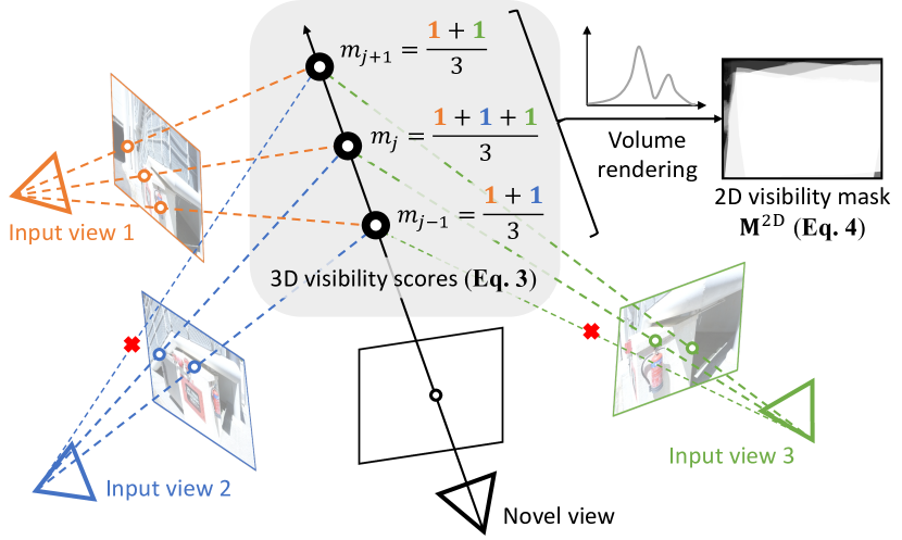
By taking $I$ reference views into account in constructing a single cost volume, the maximum number of cost volumes we can refer to is $C^{N}_{I}=\binom{N}{I}=\frac{N(N-1)\cdots(N-I+1)}{I(I-1)\cdots 1}$ for each target view, where $N$ is the number of reference views. However, utilizing all cost volumes results in high memory consumption and also leads to inefficient rendering. To tackle this challenge, we propose a method to select those cost volumes with the largest contribution to viewport coverage and potential enhancement of rendering quality for novel views. To evaluate the contribution of each cost volume, we present multi-view 3D visibility scores as a metric.

For each sample point in a cost volume, we calculate its corresponding 3D visibility scores (the gray-shaded part in Fig. 2). These scores quantify the level of observation from various cost volumes, serving as a measurement of visibility. To calculate the 3D visibility scores of a single cost volume in a rendered view, we sample rays from the rendered view and aggregate the visibility weight from the reference views. Let $I$ represent the total number of reference views. We use $\vmathbb{1}_{i}(p)$ to indicate whether a sample point $p$ is in the viewport of reference view $i$ (bottom part in Fig. 2). The 3D visibility scores $m_{j}$ are calculated using the formula:

(3) $$m_{j}=\frac{\sum_{i=1}^{I}\vmathbb{1}_{i}(p)}{I},$$

where the subscript $j$ denotes the sampled 3D point index along the ray, and the output 3D visibility scores range from 0 to 1. Each point on the mask indicates its 3D visibility score, with larger values reflecting higher confidence in the information at a specific sample point. The visibility score can be utilized as the weight for the feature of a point on a specific cost volume. Therefore, with the 3D visibility scores, we can combine the results from different cost volumes when volume rendering.

After obtaining 3D visibility scores for each cost volume, we propose the 2D visibility mask. The 2D visibility is constructed by volume rendering the 3D metrics scores to novel view, as shown in Fig. 2. Similar to Eq. 2, given ray r from the camera center $o$ with direction $d$, the value of 2D visibility mask is given by:

(4) $$\textbf{M}^{\text{2D}}(\textbf{r})=\sum_{j=1}^{J}T^{\prime}(j)\alpha\left(m_{j}\delta_{j}\right)m_{j},$$

where $T^{\prime}(j)=\exp(-\sum_{s=1}^{j-1}m_{s}\delta_{s})$ is the transmitte considering 3D visibility scores. The 2D visibility mask will be used in cost volume selection; we will thoroughly discuss it in Sec. 3.4.

Figure 3. Combined rendering from multiple cost volumes. Using a single cost volume, as in traditional MVS-based NeRFs, often introduces padding artifacts or incorrect geometry, as indicated by the red dashed circles. Our method warps selected cost volumes to the novel view’s frustum and applies 3D visibility scores $m_{j}$ as weights to blend multiple cost volumes during volume rendering. Combined rendering provides broader viewport coverage and combines information from multiple cost volumes, leading to improved image synthesis and alleviating artifacts.

3.3. Rendering by Combining Multiple Cost Volumes

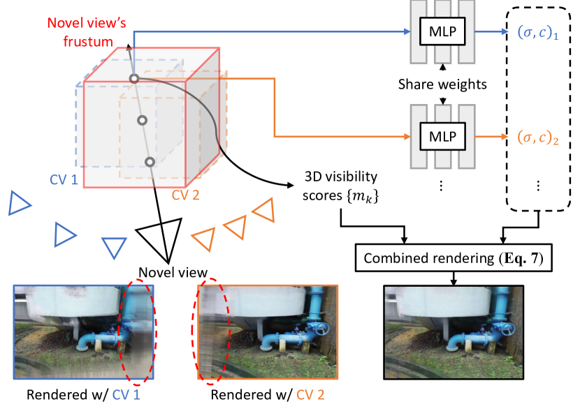
Our proposed rendering differs from the traditional one (Eq. 2) by considering 3D visibility scores and combining multiple cost volumes. Below, we explain the modifications we make. First, let us only consider a single cost volume for simplicity. The pixel color output by considering only a single cost volume is given by:

(5) $$C_{\text{single}}(\textbf{r})=\sum_{j=1}^{J}T_{\text{single}}(j)\alpha\left(\sigma_{j}\delta_{j}\right)m_{j}c_{j},$$

(6) $$T_{\text{single}}(j) =\exp\left(-\sum_{s=1}^{j-1}\left(\sigma_{s}\delta_{s}-\ln m_{s}\right)\right).$$

Please refer to the supplementary material for the derivation of the transmittance considering only a single cost volume $T_{\text{single}}(j)$.

To further consider multiple cost volumes and also utilize their corresponding 3D visibility scores, we modify Eq. 9 to combine the result across multiple cost volumes. The final proposed volume rendering is given by:

(7) $$C(\textbf{r})=\sum_{k=1}^{K}\sum_{j=1}^{J}T_{\text{combined}}(j)\alpha\left(\sigma^{k}_{j}\delta_{j}\right)M^{k}_{j}c^{k}_{j},$$

(8) $$T_{\text{combined}}(j)=\sum_{k=1}^{K}\exp\left(-\sum_{s=1}^{j-1}\left(\sigma_{s}^{k}\delta_{s}-\ln M_{s}^{k}\right)\right),$$

where $K$ is the number of selected cost volumes, and $M_{j}^{k}=\frac{m^{k}_{j}}{\sum_{k=1}^{K}m^{k}_{j}}$ is the normalized 3D visibility score so that the summation of 3D visibility scores over selected cost volumes equals 1.

The illustration and effect of combining multiple cost volumes in rendering is shown in Fig. 3. Existing MVS-based NeRFs use a single cost volume to render novel views that contain padding artifacts and wrong geometry. Combining multiple cost volumes in rendering alleviates these artifacts and broadens the viewport coverage of novel views, thus improving the rendering quality.

3.4. Support Cost Volume Set Selection

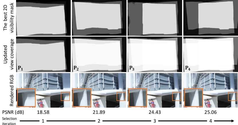
As mentioned in Sec. 3.3, we only select $K$ cost volumes for combined rendering to optimize rendering efficiency. Ideally, combining selected $K$ cost volumes should provide maximum coverage for the rendered view. This problem can be formulated as maximum coverage problem, which is NP-hard. Thus, to complete view selection in polynomial time, we propose a greedy algorithm to construct a support set $\mathbf{S}$ of $K$ cost volumes in Algorithm 1. Nemhauser et al. (Nemhauser et al., 1978) also proved that the greedy algorithm is the optimal algorithm in polynomial time.

Algorithm 1 Support cost volume set selection algorithm

0:  $\{\text{\bf{CV}}_{n}\}_{n=1}^{N}$: $N$ candidate cost volumes

0:  $\{\text{\bf{M}}^{\text{2D}}_{n}\}_{n=1}^{N}$: 2D visibility masks

0:  $\mathbf{S}$: a support set of $K$ cost volumes

1:  $\mathbf{S}\leftarrow\varnothing$ $\triangleright$ Initialize the support CV set as an empty set

2:  $\text{\bf{P}}_{0}\leftarrow\text{2D Mask filled with ones}$ $\triangleright$ Initialize the view coverage

3:  while $\left|\mathbf{S}\right|<K$ do

4:     $\text{best\_idx}\leftarrow 0$

5:     $\text{max\_ratio}\leftarrow 0$

6:     $i\leftarrow 1$ $\triangleright$ Initialize selection iteration

7:     while $i\leq N$ do

8:        if $\text{\bf{CV}}_{i}\not\in\mathbf{S}$ then $\triangleright$ Consider remaining views only

9:           $\text{ratio}\leftarrow\sum{(\text{\bf{P}}_{i-1}\cdot\text{\bf{M}}^{\text{2D}}_{i})}$

10:           if $\text{ratio}>\text{max\_ratio}$ then

11:              $\text{max\_ratio}\leftarrow\text{ratio}$

12:              $\text{best\_idx}\leftarrow i$

13:           end if

14:        end if

15:        $i\leftarrow i+1$

16:     end while

17:     $\text{\bf{P}}_{i}\leftarrow\text{\bf{P}}_{i-1}\cdot(1-\text{\bf{M}}^{\text{2D}}_{{\text{best\_idx}}})$ $\triangleright$ Update the view coverage

18:     $\mathbf{S}\leftarrow\mathbf{S}\cup\{\text{\bf{CV}}_{\text{best\_idx}}\}$ $\triangleright$ Add the best CV to the set

19:  end while

We show an example of the proposed selection algorithm in Fig. 4. At the beginning of the algorithm, our method selects the cost volume with the largest coverage score of the corresponding 2D visibility mask. The rendered image contains padding artifacts near the image boundaries as the viewport of this single cost volume is limited. Later on, our selection algorithm gradually selects the cost volumes that could maximize the visibility coverage and, therefore, enlarge the valid region of the rendered view. As a result, the rendering quality of novel views progressively grows as more cost volumes are selected and combined in the volume rendering.

Figure 4. Support cost volume set selection. Initially, our greedy algorithm selects a single cost volume, providing maximum coverage yet insufficient to prevent padding artifacts (orange boxes). Subsequent iterations incorporate additional cost volumes, progressively expanding view coverage, and improving image quality, as indicated by the increasing PSNR values.

3.5. End-to-end Fine-tuning

Our method is compatible with any MVS-based NeRFs to boost the rendering quality. Moreover, our approach is not optimized for a specific scene and could be generalized to new scenes, allowing it to enhance any end-to-end fine-tunable model. Fine-tuning refines geometry and color consistency within cost volumes and eliminates padding artifacts through combined rendering from multiple cost volumes. Thus, our method could augment the capabilities of advanced MVS-based NeRFs beyond ENeRF and MVS-NeRF. Please refer to the supplementary material for the fine-tuning details.

4. Experiments

4.1. Experimental Settings

Datasets.

We evaluate two datasets: (1) the Free dataset collected by F2-NeRF (Wang et al., 2023b) and (2) the ScanNet (Dai et al., 2017) dataset. The Free dataset consists of seven challenging scenes featuring narrow, long camera trajectories and focused foreground objects. Our evaluations on the Free dataset follow the train/test split in F2-NeRF (Wang et al., 2023b) by using one-eighth of the images for testing and the rest for training. As for the ScanNet dataset, we strictly follow the train/test splits as defined in NeRFusion (Zhang et al., 2022), NerfingMVS (Wei et al., 2021), and SurfelNeRF (Gao et al., 2023), with eight large-scale indoor scenes. We assess the rendering quality with PSNR, SSIM (Wang et al., 2004), and LPIPS (Zhang et al., 2018) metrics.

Baselines.

We compare BoostMVSNeRFs with various state-of-the-art NeRFs, including fast per-scene optimization NeRFs such as F2-NeRF (Wang et al., 2023b) and Zip-NeRF (Barron et al., 2023) and generalizable NeRFs such as MVSNeRF (Chen et al., 2021), ENeRF (Lin et al., 2022) and SurfelNeRF (Gao et al., 2023).

In particular, F2-NeRF excels in outdoor scenes with free camera trajectories. Our method employs cost volume representations similar to MVSNeRF and ENeRF but enlarges valid visible regions by fusing multiple cost volumes. Although SurfelNeRF also proposes fusing multiple surfels as a type of 3D representation, the fusion method and its scene representation differ from BoostMVSNeRFs. To ensure fairness, we used the same experimental settings as in previous studies and used official codes where possible. All the training, fine-tuning, and evaluations are done on a single RTX 4090 GPU.

Our method is compatible with MVS-based techniques, allowing us to employ pre-trained models such as MVSNeRF and ENeRF in our experiments. Unless otherwise specified, we use ENeRF as our backbone MVS-based NeRF method in all the experiments. We optimize the parameters, $N=6$, $I=3$, and $K=4$, for efficient rendering and high quality. Our method achieves similar runtime performance in rendering and fine-tuning as other generalizable NeRF methods but renders significantly improved quality. Additional implementation details of the proposed BoostMVSNeRFs, such as the sensitivity analysis of the number of selected cost volumes $K$ and the numerical representation (continuous or binary) of 2D visibility masks, are provided in the supplementary material.

4.2. Comparison with State-of-the-art Methods

Table 1. Quantitative comparisons with state-of-the-art methods on the Free (Wang et al., 2023b) dataset.

Method	Setting	PSNR $\uparrow$	SSIM $\uparrow$	LPIPS $\downarrow$	FPS $\uparrow$
MVSNeRF (Chen et al., 2021)	No per-scene optimization	20.06	0.721	0.469	1.79
MVSNeRF + Ours		20.52	0.722	0.470	1.26
ENeRF (Lin et al., 2022)		23.24	0.844	0.225	9.90
ENeRF+Ours		24.21	0.862	0.218	5.51
F2-NeRF (Wang et al., 2023b)	Per-scene optimization	25.55	0.776	0.278	3.75
Zip-NeRF (Barron et al., 2023)		25.90	0.772	0.241	0.66
$\text{MVSNeRF}_{\text{ft}}$ (Chen et al., 2021)		20.49	0.698	0.425	1.79
MVSNeRF + $\text{Ours}_{\text{ft}}$		21.59	0.759	0.265	1.26
$\text{ENeRF}_{\text{ft}}$ (Lin et al., 2022)		25.19	0.880	0.180	9.90
$\text{ENeRF+Ours}_{\text{ft}}$		26.14	0.894	0.171	5.51

Free dataset.

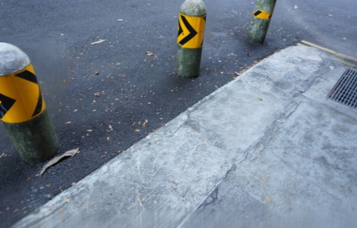
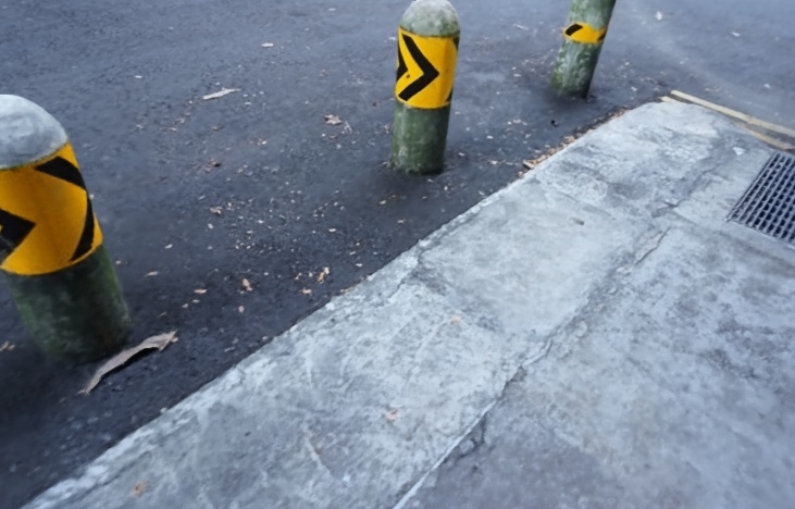
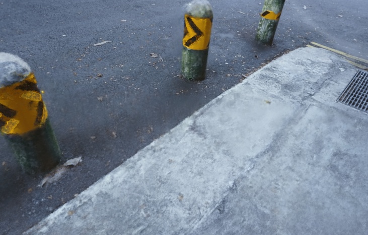
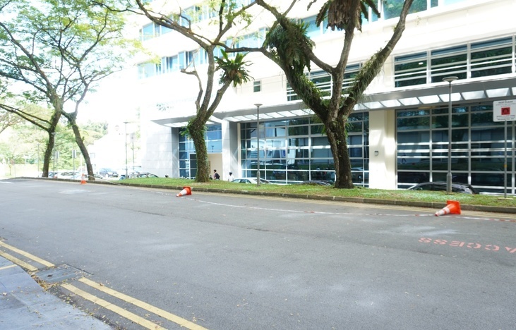
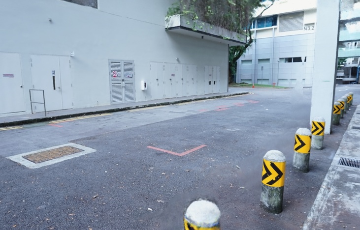
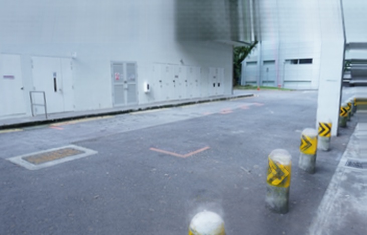
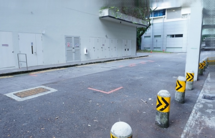
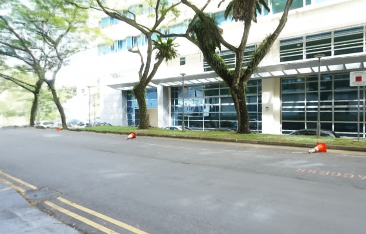
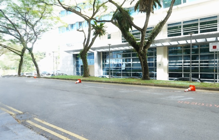
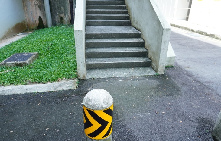
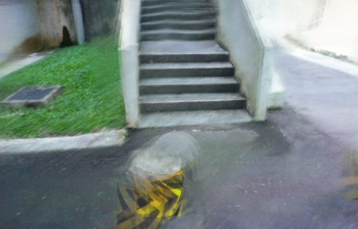
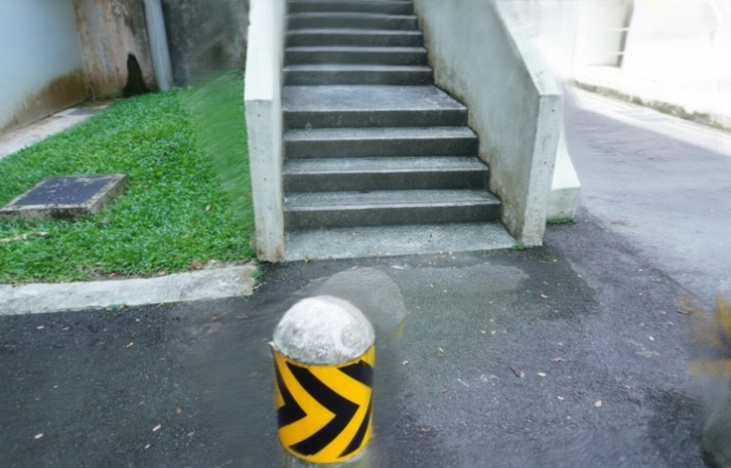
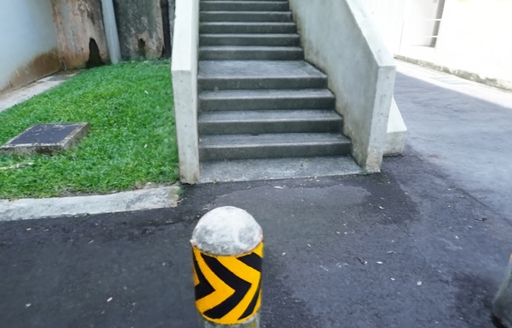
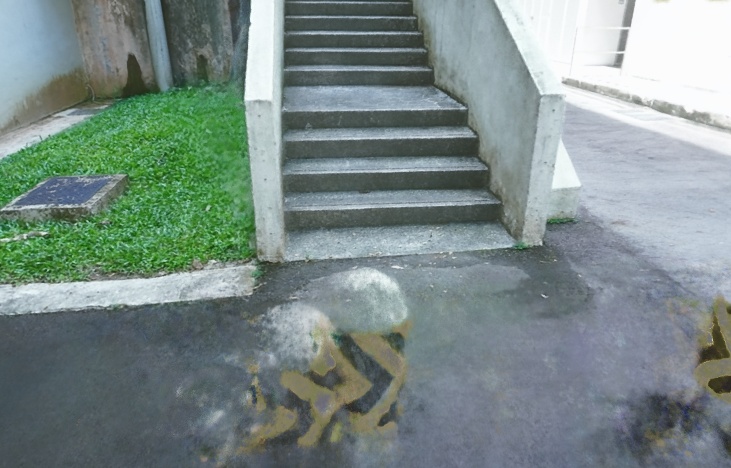
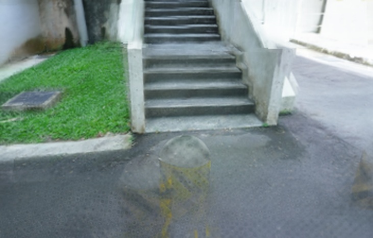
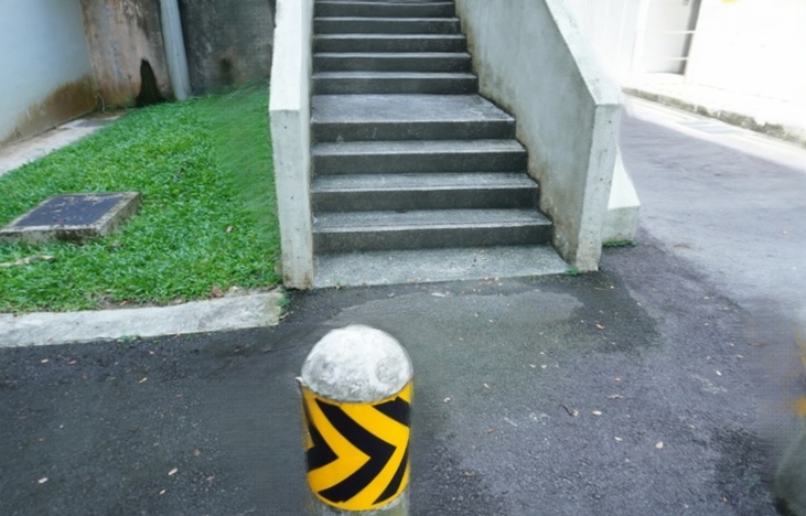
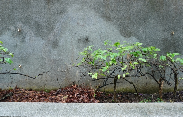
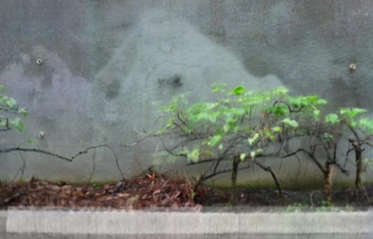
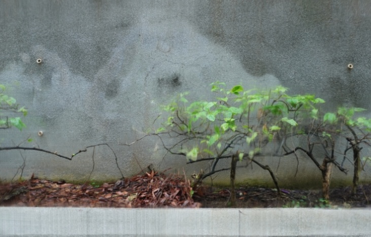
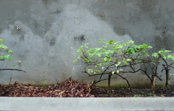
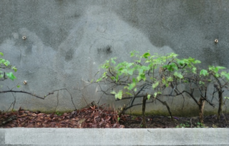
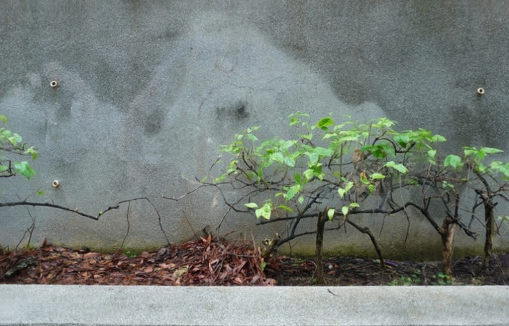
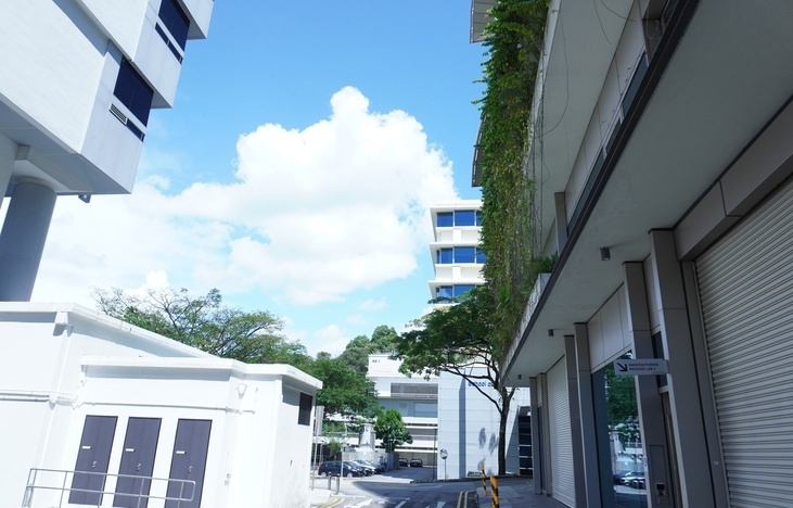
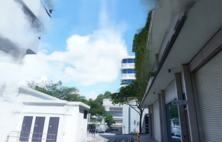
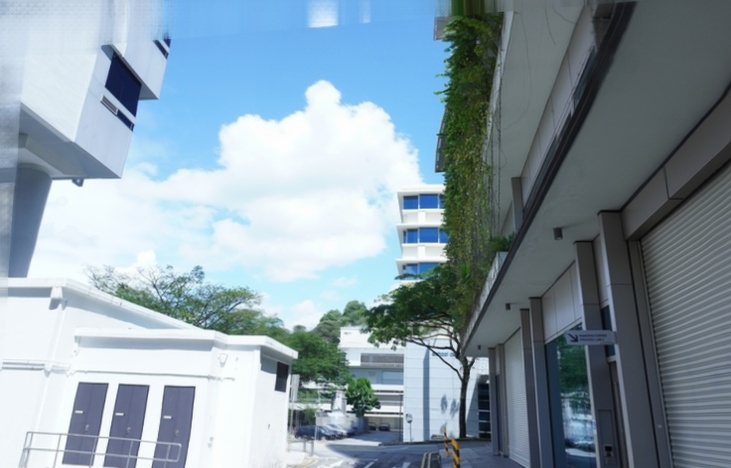
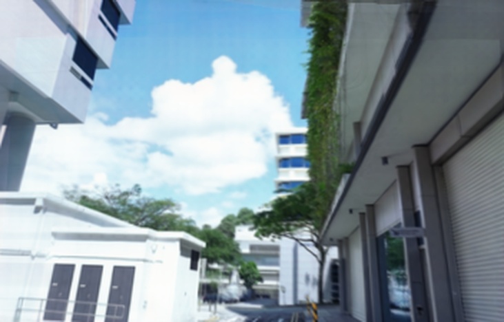
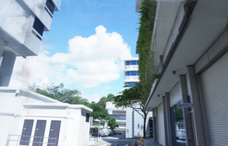
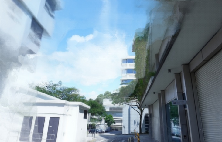
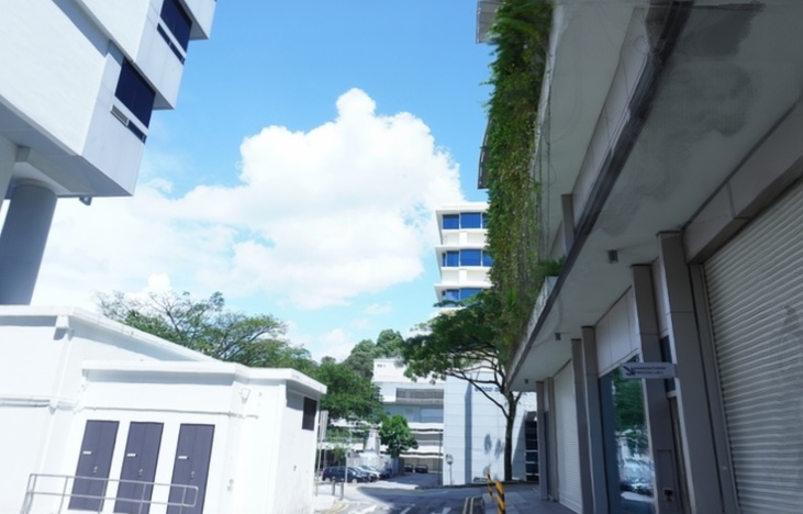
On the Free dataset, BoostMVSNeRFs emerges as the best among no per-scene and per-scene optimization NeRF methods as shown in Table 1 and Fig. 5. Compared to F2-NeRF and SurfelNeRF, which produced blurred images, BoostMVSNeRFs leverages multiple cost volume fusion and view selection based on visibility maps for superior rendering quality. Our method demonstrates compatibility with various camera trajectories and achieves results comparable to those of existing methods.

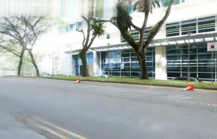
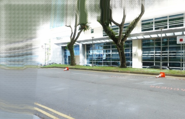
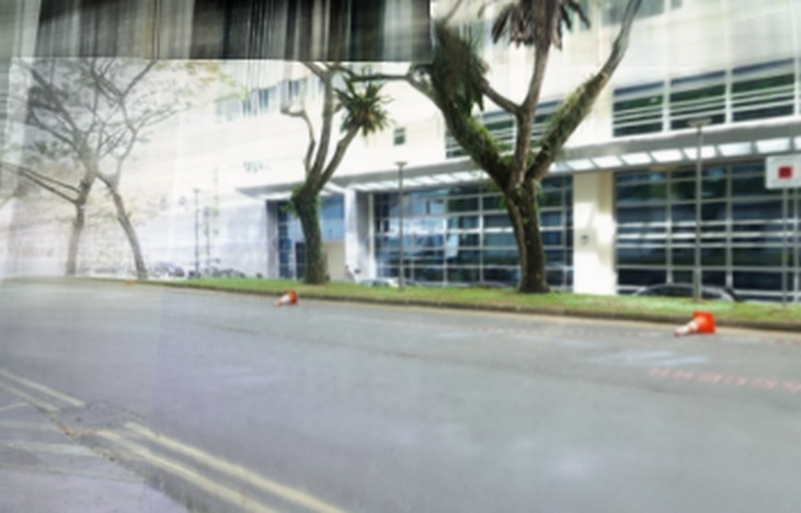
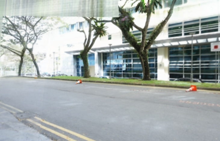
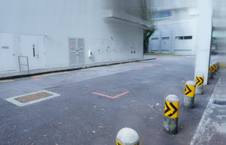
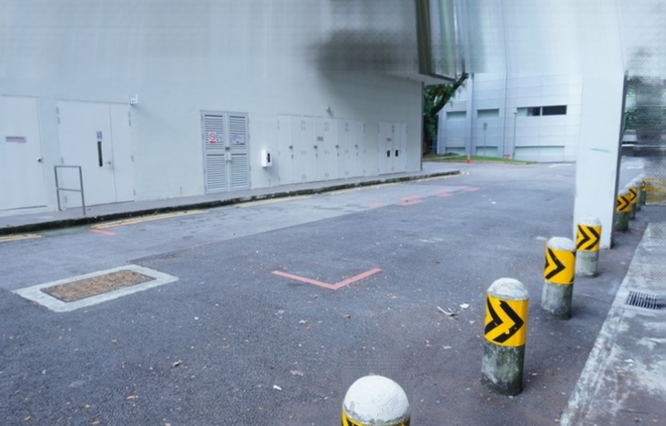
Our method outperforms generalizable NeRF techniques like MVSNeRF and ENeRF on the Free dataset (Table 1), enhancing rendering quality through our view selection and multiple cost volume combined rendering approach. Integrated with MVS-based NeRFs, our method achieves a PSNR improvement of 0.5-1.0 dB without requiring additional training. End-to-end fine-tuning on test scenes further enhances rendering quality, particularly in regions where a single cost volume falls short. This highlights the benefit of multiple-cost volume fusion. For detailed visual comparisons, please refer to Fig. 6, 9, 10, and the supplementary material.

	No per-scene optimization		Per-scene optimization
Ground truth	MVSNeRF	Ours	F2-NeRF	Zip-NeRF	MVSNeRF + ft	Ours + ft
	(Chen et al., 2021)		(Wang et al., 2023b)	(Barron et al., 2023)	(Chen et al., 2021)

Figure 5. Qualitative comparisons of rendering quality on the Free (Wang et al., 2023b) dataset.

Ground truth	MVSNeRF (Chen et al., 2021)	MVSNeRF + ft	ENeRF (Lin et al., 2022)	ENeRF + ft
	MVSNeRF + ours	MVSNeRF + ours + ft	ENeRF + ours	ENeRF + ours + ft

Figure 6. Qualitative rendering quality improvements of integrating our method into MVS-based NeRF methods on the Free dataset.

Table 2. Quantitative comparisons with state-of-the-art methods on the ScanNet (Dai et al., 2017) dataset.

Method	Setting	PSNR $\uparrow$	SSIM $\uparrow$	LPIPS $\downarrow$	FPS $\uparrow$
SurfelNeRF (Gao et al., 2023)	No per-scene optimization	19.28	0.623	0.528	1.25
MVSNeRF (Chen et al., 2021)		23.40	0.862	0.367	1.99
MVSNeRF + Ours		23.66	0.872	0.365	1.41
ENeRF (Lin et al., 2022)		31.73	0.955	0.206	11.03
ENeRF + Ours		31.01	0.957	0.219	6.14
F2-NeRF (Wang et al., 2023b)	Per-scene optimization	28.11	0.894	0.230	4.18
$\text{SurfelNeRF}_{\text{ft}}$ (Gao et al., 2023)		20.04	0.653	0.504	1.25
Zip-NeRF (Barron et al., 2023)		32.24	0.917	0.214	0.74
$\text{MVSNeRF}_{\text{ft}}$ (Chen et al., 2021)		24.69	0.872	0.316	1.99
MVSNeRF + $\text{Ours}_{\text{ft}}$		24.63	0.880	0.320	1.41
$\text{ENeRF}_{\text{ft}}$ (Lin et al., 2022)		32.70	0.960	0.174	11.03
$\text{ENeRF + Ours}_{\text{ft}}$		32.87	0.955	0.173	6.14

ScanNet dataset.

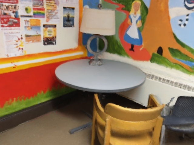
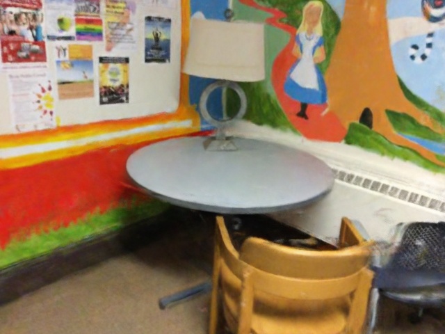
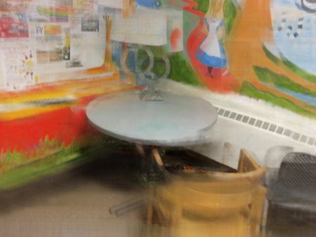
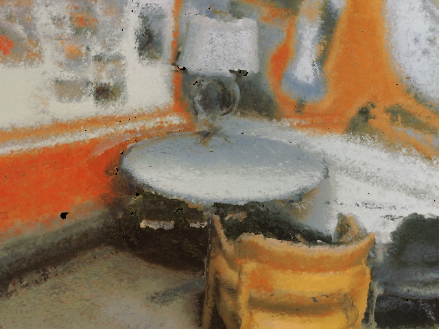
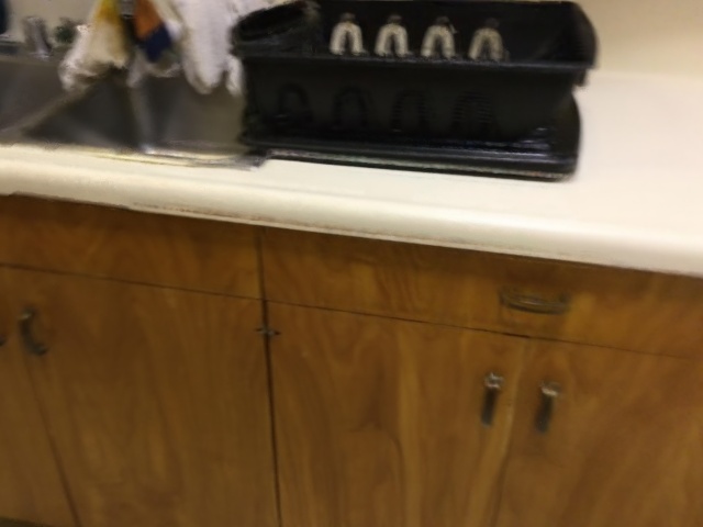
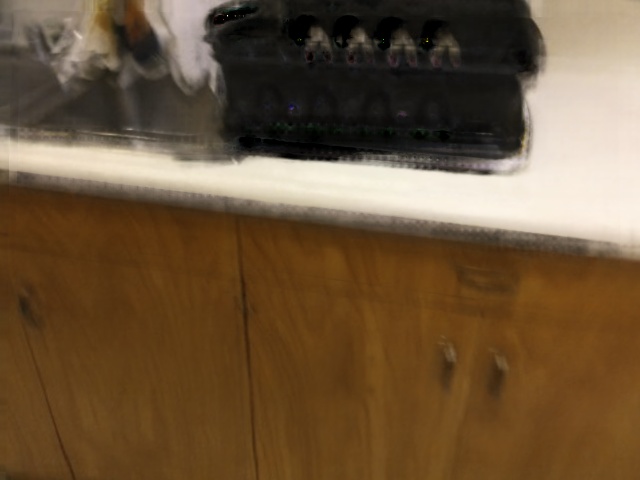
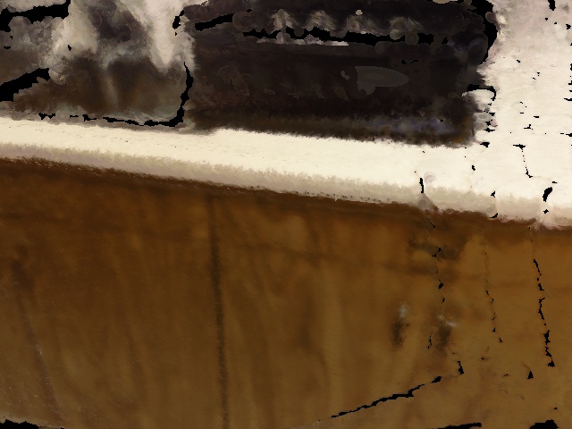
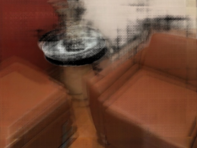
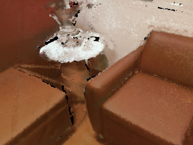
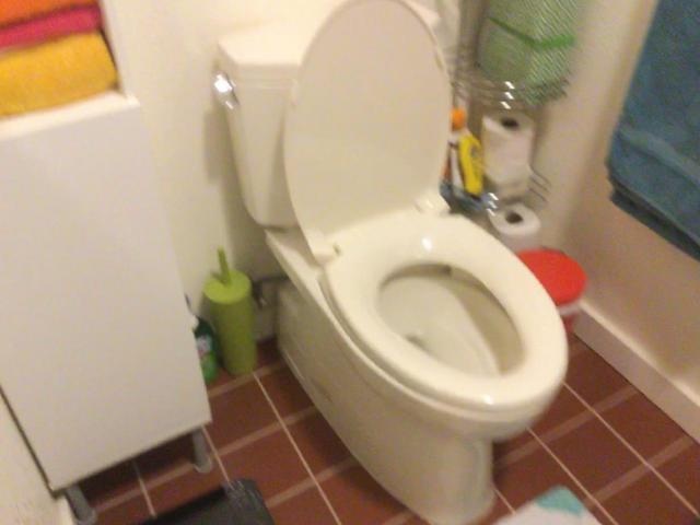
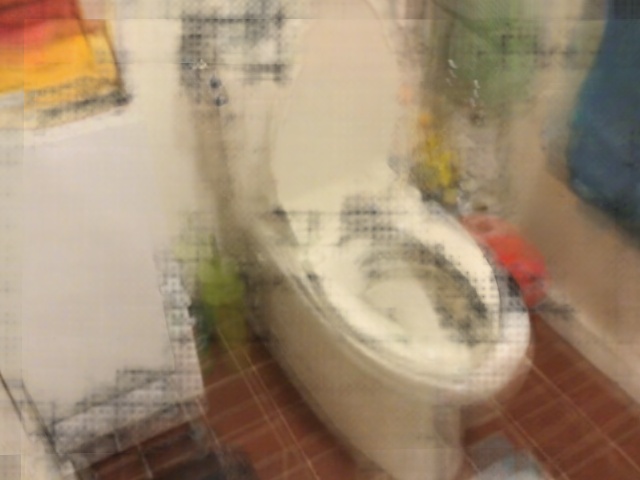
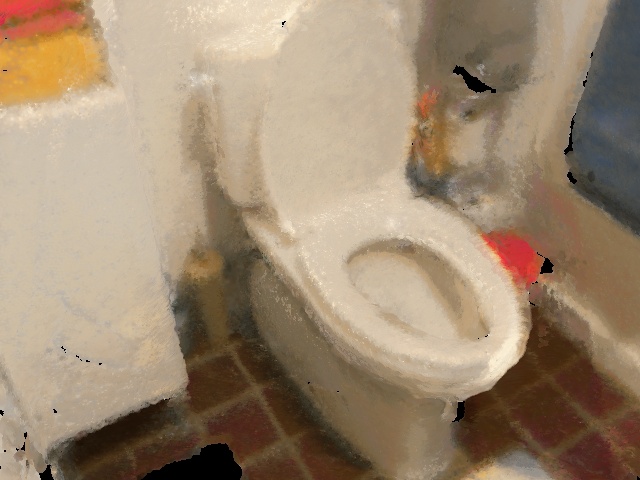
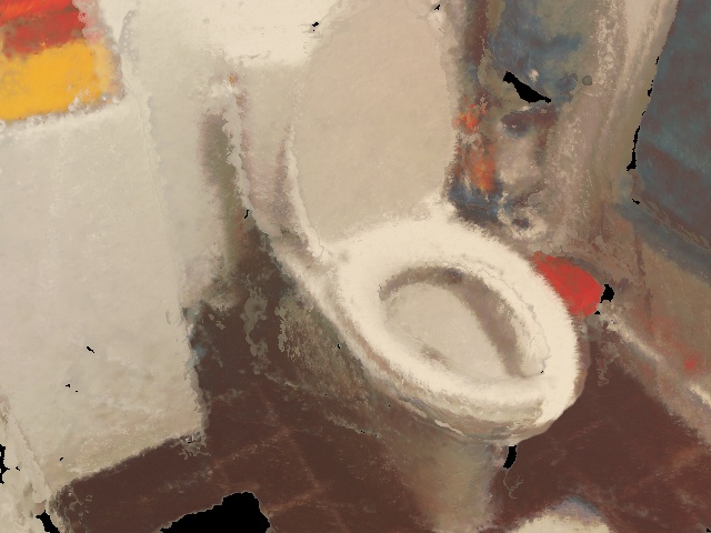
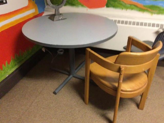
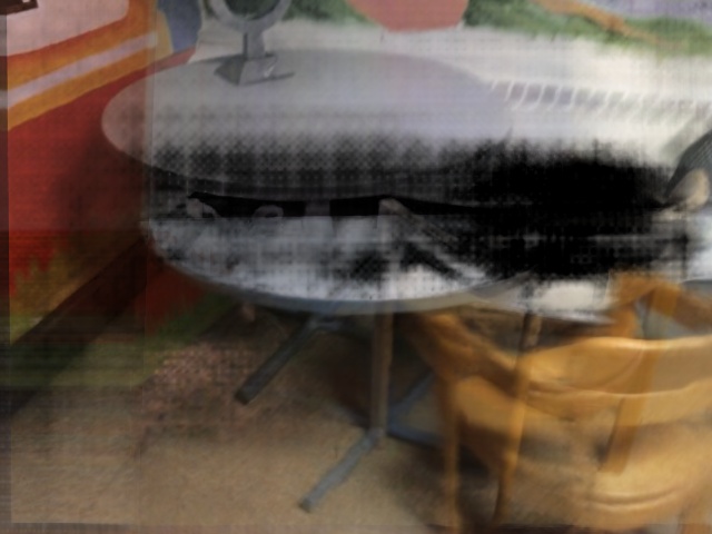
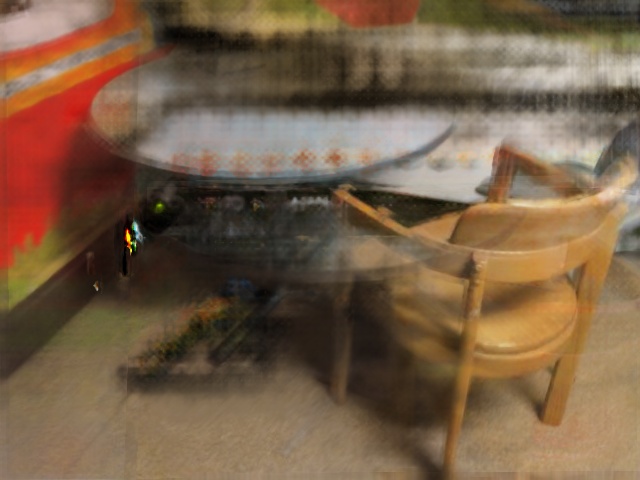
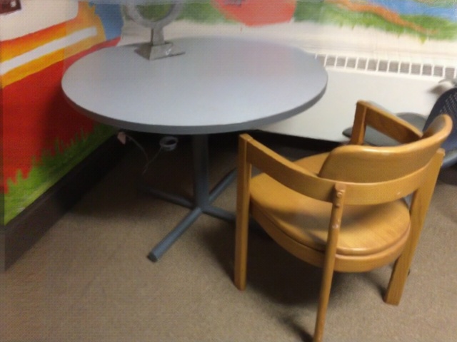
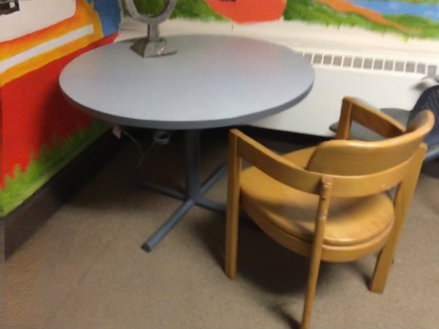
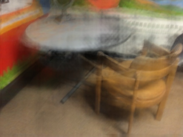
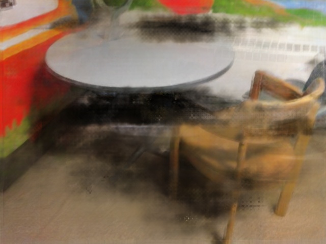
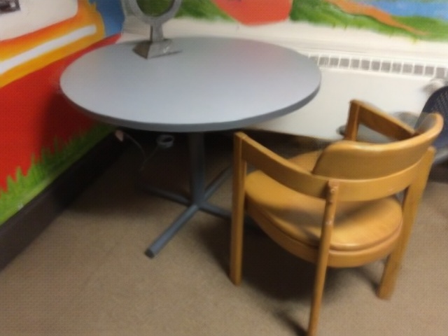
We conducted a comprehensive comparison of BoostMVSNeRFs with other state-of-the-art methods in no per-scene and per-scene optimization settings on the ScanNet dataset in Table 2. BoostMVSNeRFs demonstrates superior performance with a PSNR of 31.73 dB in no per-scene optimization, outperforming SurfelNeRF due to its cost volume fusion and efficient view selection strategy. In per-scene optimization, BoostMVSNeRFs excels again with a PSNR of 32.87 dB, indicating its effectiveness in cost volume fusion and per-scene adaptation. We also compare our method with two generalizable NeRF methods, MVSNeRF and ENeRF, on the ScanNet dataset in Table 2 and Fig. 12. Our method achieves better rendering quality over existing MVS-based NeRF methods in SSIM without per-scene optimization and in PSNR and LPIPS with per-scene fine-tuning.

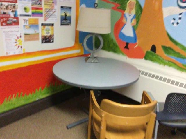
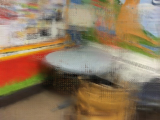
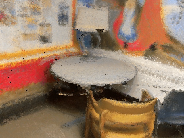
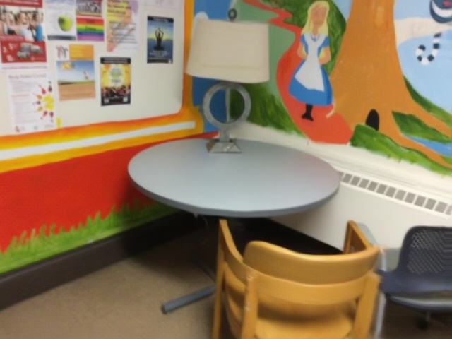
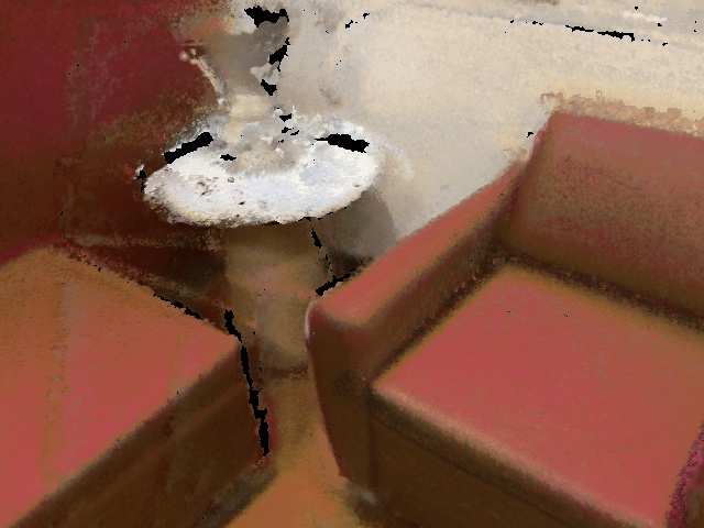
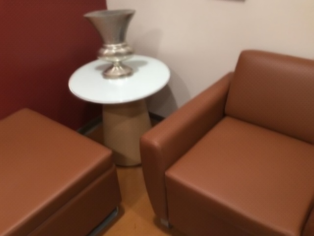
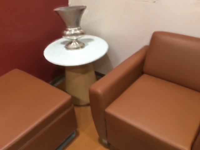
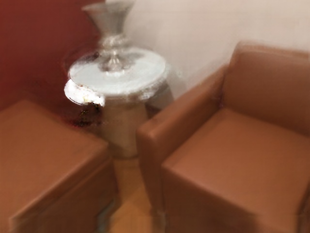
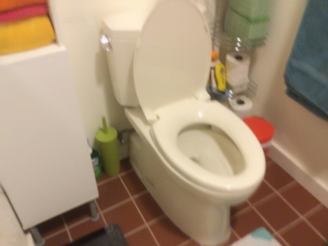
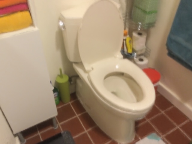
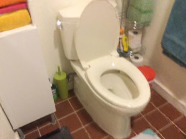
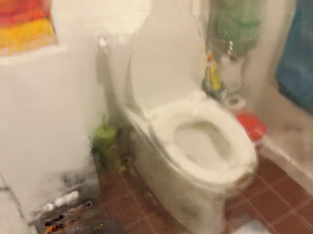
Furthermore, our approach showed impressive results on large-scale scenes, outperforming SurfelNeRF in both direct inference and per-scene fine-tuning. Unlike SurfelNeRF, which suffered from artifacts due to its surfel-based rendering approach, our model’s multiple cost volume fusion and efficient view information selection and aggregation led to high-quality and consistent renderings, as shown in Fig. 5. This indicates our cost volume fusion’s effectiveness in reconstructing large-scale scenes efficiently and accurately.

4.3. Ablation Study

Cost volume selection scheme.

In Sec. 3.4, we propose a greedy method to select the cost volumes that will approximately maximize the view coverage. To validate the effectiveness of our method, We conducted experiments comparing two other cost volume selection methods. These two methods are: (a) selecting $K$ cost volumes that are closest to the render view pose, which is adopted by ENeRF (Lin et al., 2022) and (b) selecting corresponding cost volumes directly with the highest contribution of 2D visibility mask. In particular, method (b) is a degenerate version of method our proposed selection method (c), which is based on view coverage. Table 3 shows that our greedy cost volume selection method performs better than the other two methods.

Table 3. Ablation of the cost volume selection. We compare three different strategies for cost volume selection on all scenes of the Free (Wang et al., 2023b) dataset: (a) ENeRF’s method, which is based on pose distance, (b) direct selection of cost volumes with maximum visibility, and (c) Our proposed greedy method, which maximizes the visibility coverage.

Method	PSNR $\uparrow$	SSIM $\uparrow$	LPIPS $\downarrow$
(a) ENeRF (Lin et al., 2022)	24.09	0.861	0.220
(b) Maximize 2D visibility $\textbf{M}^{\text{2D}}_{i}$	24.19	0.861	0.218
(c) Maximize view coverage $\textbf{P}_{i}$	24.21	0.862	0.218

Single cost volume with more input views vs. Combining multiple cost volumes

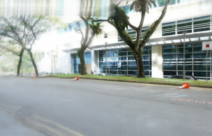
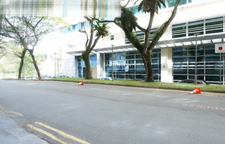
In our method, we select multiple cost volumes and combine them in volume rendering, while ENeRF only forms one cost volume. To examine our method’s effectiveness, we train ENeRF (originally three input views) with more input views (6 in this ablation, in order to evenly compare with our proposed method). The results are shown in Table 4 and Fig. 7. We can see an increase in the number of input views which requires time-consuming training to construct a single cost volume. However, the rendering quality improvements are subtle both with or without per-scene fine-tuning. In contrast, our cost volume selection method and combined rendering scheme improve the rendering quality by a large margin and could be further optimized with per-scene fine-tuning.

Table 4. Different ways of combining more input views. We compare training an MVS-based NeRF with a larger number of input views (6 input views here) and our proposed cost volume selection and combined rendering on all scenes of the Free (Wang et al., 2023b) dataset.

Method	Setting	PSNR $\uparrow$	SSIM $\uparrow$	LPIPS $\downarrow$
$\text{ENeRF}^{\text{3-view}}$ (Lin et al., 2022)	No per-scene optimization	23.24	0.844	0.225
$\text{ENeRF}^{\text{6-view}}$ (Lin et al., 2022)		23.53	0.770	0.231
$\text{ENeRF}^{\text{3-view}}$ + Ours		24.21	0.862	0.218
$\text{ENeRF}^{\text{3-view}}_{\text{ft}}$ (Lin et al., 2022)	Per-scene optimization	25.19	0.880	0.180
$\text{ENeRF}^{\text{6-view}}_{\text{ft}}$ (Lin et al., 2022)		25.61	0.840	0.172
$\text{ENeRF}^{\text{3-view}}$ + $\text{Ours}_{\text{ft}}$		26.14	0.894	0.171

	$\text{ENeRF}^{\text{3-view}}$	$\text{ENeRF}^{\text{6-view}}$	$\text{ENeRF}^{\text{3-view}}$ + Ours
Ground truth	$\text{ENeRF}^{\text{3-view}}_{\text{ft}}$	$\text{ENeRF}^{\text{6-view}}_{\text{ft}}$	$\text{ENeRF}^{\text{3-view}}$ + $\text{Ours}_{\text{ft}}$

Figure 7. Visual effects of different ways of combining more input views. Artifacts in disocclusion regions cannot be resolved by including more input views for a single cost volume. Our method could alleviate these artifacts by combining more cost volumes in rendering.

Robustness with sparse input views.

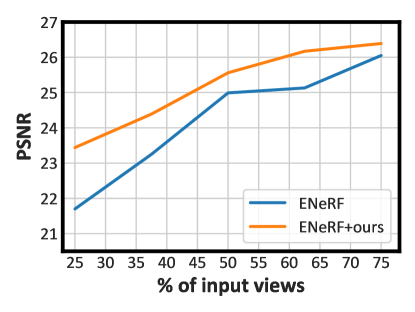
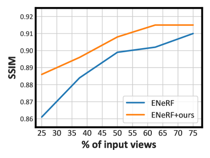
Our proposed combined rendering from multiple cost volumes addresses the challenges of reconstructing large-scale and unbounded scenes due to broader viewport coverage. Therefore, our method could be more robust to sparse input views as more and farther cost volumes are considered during rendering. We conduct an experiment comparing performance across various degrees of sparse views to demonstrate the robustness of our method with sparse input views. Specifically, we uniformly sub-sample the training views and evaluate the rendering quality. The results show a more significant decline in both PSNR and SSIM for ENeRF compared to ours while input views become sparse, as indicated by the curve in figure 8.

Figure 8. Robustness with sparse input views. With more sparse input views, the performance drop of our method is less severe than ENeRF, demonstrating the robustness of our method against sparse input views by combining multiple cost volumes in rendering.

5. Conclusion

In summary, our BoostMVSNeRFs enhances MVS-based NeRFs, tackling large-scale and unbounded scene rendering challenges. Utilizing 3D visibility scores for multi-cost volume integration, BoostMVSNeRFs synthesizes significantly better novel views, enhancing viewport coverage and minimizing typical single-cost volume artifacts. Compatible with current MVS-based NeRFs, BoostMVSNeRFs supports end-to-end training for scene-specific enhancement. Experimental results validate the efficacy of our method in boosting advanced MVS-based NeRFs, contributing to more scalable and high-quality view synthesis. Future work will focus on reducing MVS dependency and optimizing memory usage, furthering the field of neural rendering for virtual and augmented reality applications.

	No per-scene optimization		Per-scene optimization
Ground truth	MVSNeRF	Ours	F2-NeRF	Zip-NeRF	MVSNeRF + ft	Ours + ft
	(Chen et al., 2021)		(Wang et al., 2023b)	(Barron et al., 2023)	(Chen et al., 2021)

Figure 9. Qualitative comparisons of rendering quality on the Free (Wang et al., 2023b) dataset.

Ground truth	MVSNeRF (Chen et al., 2021)	MVSNeRF + ft	ENeRF (Lin et al., 2022)	ENeRF + ft
	MVSNeRF + ours	MVSNeRF + ours + ft	ENeRF + ours	ENeRF + ours + ft
Ground truth	MVSNeRF (Chen et al., 2021)	MVSNeRF + ft	ENeRF (Lin et al., 2022)	ENeRF + ft
	MVSNeRF + ours	MVSNeRF + ours + ft	ENeRF + ours	ENeRF + ours + ft

Figure 10. Qualitative rendering quality improvements of integrating our method into MVS-based NeRF methods on the Free dataset.

	No per-scene optimization			Per-scene optimization
Ground truth	MVSNeRF	SurfelNeRF	Ours	F2-NeRF	Zip-NeRF	MVSNeRF + ft	SurfelNeRF + ft	Ours + ft
	(Chen et al., 2021)	(Gao et al., 2023)		(Wang et al., 2023b)	(Barron et al., 2023)	(Chen et al., 2021)	(Gao et al., 2023)

Figure 11. Qualitative comparisons of rendering quality on the ScanNet (Dai et al., 2017) dataset.

Ground truth	MVSNeRF (Chen et al., 2021)	MVSNeRF + ft	ENeRF (Lin et al., 2022)	ENeRF + ft
	MVSNeRF + ours	MVSNeRF + ours + ft	ENeRF + ours	ENeRF + ours + ft
Ground truth	MVSNeRF (Chen et al., 2021)	MVSNeRF + ft	ENeRF (Lin et al., 2022)	ENeRF + ft
	MVSNeRF + ours	MVSNeRF + ours + ft	ENeRF + ours	ENeRF + ours + ft

Figure 12. Qualitative rendering quality improvements of integrating our method into MVS-based NeRF methods on the ScanNet dataset.

Appendix A Appendix Overview

This supplementary material presents additional results to complement the main paper. First, we provide the detailed derivation of the combined volume rendering equation with multiple cost volumes in Sec. B. Then, we describe all the implementation details of BoostMVSNeRFs and baseline methods in Sec. C. Next, we show additional ablation studies, including the sensitivity analysis on the number of selected cost volumes and the effect of combining multiple cost volumes in 2D or in the 3D space in Sec. D. Finally, we provide complete quantitative evaluations and additional qualitative comparisons in Sec. E and Sec. F, respectively. In addition to this document, we provide video results of our method and state-of-the-art methods and show the rendering quality comparison.

Appendix B Derivation of the Combined Volume Rendering with Multiple Cost Volumes

Our proposed rendering differs from the traditional one by considering 3D visibility scores and combining multiple cost volumes. Below, we explain the modifications we make. First, let us only consider a single cost volume for simplicity. The pixel color output is given by:

(9) $$C_{\text{single}}(\textbf{r})=\sum_{j=1}^{J}T_{\text{single}}(j)\alpha\left(\sigma_{j}\delta_{j}\right)m_{j}c_{j},$$

(10) $$T_{\text{single}}(j) =\prod_{s=1}^{j-1}\exp\left(-\sigma_{s}\delta_{s}\right)m_{s}$$

(11) $$=\prod_{s=1}^{j-1}\exp\left(-\sigma_{s}\delta_{s}\right)\exp\left(\ln m_{s}\right)$$

(12) $$=\prod_{s=1}^{j-1}\exp\left(-\left(\sigma_{s}\delta_{s}-\ln m_{s}\right)\right)$$

(13) $$=\exp\left(-\sum_{s=1}^{j-1}\left(\sigma_{s}\delta_{s}-\ln m_{s}\right)\right).$$

To further consider multiple cost volumes and also utilize their corresponding 3D visibility scores, we modify Eq. 9 to combine the result across multiple cost volumes. The final proposed volume rendering is given by:

(14) $$C(\textbf{r})=\sum_{k=1}^{K}\sum_{j=1}^{J}T_{\text{combined}}(j)\alpha\left(\sigma^{k}_{j}\delta_{j}\right)M^{k}_{j}c^{k}_{j},$$

(15) $$T_{\text{combined}}(j)=\sum_{k=1}^{K}\exp\left(-\sum_{s=1}^{j-1}\left(\sigma_{s}^{k}\delta_{s}-\ln M_{s}^{k}\right)\right),$$

(16) $$M_{j}^{k}=\frac{m^{k}_{j}}{\sum_{k=1}^{K}m^{k}_{j}},$$

where $K$ is the number of selected cost volumes, and $M_{j}^{k}$ is the normalized 3D visibility score so that the summation of 3D visibility scores over selected cost volumes equals 1.

Appendix C Implementation Details

Our method is compatible with MVS-based NeRF techniques, allowing us to employ pre-trained models such as MVSNeRF and ENeRF in our experiments. For per-scene optimization, we fine-tune our methods with 11,000 iterations, following the settings of ENeRF, with an initial learning rate of $5e^{-4}$ and an exponential scheduler. This fine-tuning process typically takes between 1 to 2 hours on an RTX 4090 GPU, depending on the image resolution.

For a fair comparison across methods, we evaluate them using a 731 x 468 image resolution in the Free dataset and a $640\times 480$ image resolution in the ScanNet dataset. During fine-tuning, we use a resolution of $736\times 480$ to match our model architecture and subsequently downsample the images to $731\times 468$ for fair comparison.

In practical terms, both ENeRF and our models are configured with 2 samples per ray. When integrating MVSNeRF, we use 32 samples per ray to evaluate its generalizable rendering model; however, during fine-tuning, this is reduced to 8 samples per ray to address convergence issues. We employ 4 cost volumes (K=4) for combined rendering with multiple cost volumes. . For each rendering view in both datasets, we consider its nearest 6 training views ($N=6$) and build $C^{N}_{3}$ cost volumes and select $K$ best cost volumes for our method.

Appendix D Additional Ablation Studies

D.1. Sensitivity analysis on the number of selected cost volumes

In our approach, we introduce a greedy method for cost volume selection for fusion, enabling the integration of multiple cost volumes. To optimize the most effective cost volume fusion strategy, we conduct experiments by considering $K$ cost volumes during volume rendering. We explore scenarios where $K$ equals 1, 2, 3, 4, and 5, and present the corresponding results in Table 5.

Table 5. Sensitivity analysis on the number of selected cost volumes for combination. We compare the rendering quality of different numbers of selected cost volumes for combined rendering on all scenes of the Free (Wang et al., 2023b) dataset. The rendering quality improves with more cost volumes selected in combined rendering.

Method	Setting	PSNR $\uparrow$	SSIM $\uparrow$	LPIPS $\downarrow$
$K=1$	No per-scene optimization	24.05	0.865	0.205
$K=2$		24.55	0.872	0.202
$K=3$		24.68	0.875	0.202
$K=4$		24.75	0.875	0.202
$K=5$		24.79	0.875	0.203

D.2. Continuous-valued 3D visibility scores.

Our method represents 3D visibility scores with continuous values. We conduct experiments comparing our method with binary-valued 3D visibility scores, i.e., each score can only be either 0 or 1. The binary-valued 3D visibility scores $m_{j}^{\prime}$ are calculated by $m_{j}^{\prime}=1-\prod_{i=1}^{V}(1-\mathbb{1}_{i}(p))$, where $m_{j}^{\prime}$ is the binary-valued 3D visibility scores.

Table 6. Effect of continuous or binary 3D visibility scores. We compare representing the 3D visibility score using binary values with our continuous values on all scenes of the Free (Wang et al., 2023b) dataset. Representing 3D visibility scores with continuous values performs better than binary values.

Method	Setting	PSNR $\uparrow$	SSIM $\uparrow$	LPIPS $\downarrow$
Discrete mask	No per-scene optimization	24.05	0.855	0.227
Continuous mask (Ours)		24.21	0.862	0.218

Table 7. Ablation on different combined methods with multiple cost volumes. We compare the rendering quality between different combined methods on all scenes of the ScanNet dataset. Combined rendering in 3D performs slightly better than in the 2D space.

Method	PSNR $\uparrow$	SSIM $\uparrow$	LPIPS $\downarrow$
3D visibility scores as multipliers on densities	17.60	0.767	0.549
Rendered images and 2D visibility masks	24.20	0.868	0.360
Sampled 3D points and 3D visibility scores (Ours)	24.22	0.868	0.361

D.3. Different combined methods with multiple cost volumes

In our method, we use calculated 3D visibility scores as weights to combine multiple cost volumes during rendering. A straightforward variant is to multiply the 3D visibility scores onto queried density values in volume rendering. Yet another way is to blend rendering results from different cost volumes in the 2D image domain instead of 3D sampled points. Table 7 demonstrates that our combination method using 3D sampled points and 3D visibility scores achieves the best rendering quality.

Appendix E Complete Quantitative Evaluations

E.1. Free dataset

We show all 7 scenes of the quantitative comparisons on the Free (Wang et al., 2023b) dataset in Table 8.

Table 8. Complete quantitative comparisons with state-of-the-art methods on the Free (Wang et al., 2023b) dataset.

Method	Setting	Hydrant	Lab	Pillar	Road	Sky	Stair	Grass
		PSNR $\uparrow$
MVSNeRF (Chen et al., 2021)	No per-scene optimization	19.63	20.11	19.58	20.84	18.58	21.98	19.69
MVSNeRF + Ours		20.21	20.00	20.02	21.77	19.50	21.64	20.47
ENeRF (Lin et al., 2022)		21.85	23.48	24.3	24.73	22.27	25.52	20.53
ENeRF + Ours		22.73	23.94	26.06	25.88	23.44	25.78	21.64
F2-NeRF (Wang et al., 2023b)	Per-scene optimization	23.75	24.34	28.05	26.03	25.10	28.14	23.44
Zip-NeRF (Barron et al., 2023)		25.43	27.94	25.30	28.83	27.12	28.21	18.46
$\text{MVSNeRF}_{\text{ft}}$ (Chen et al., 2021)		19.33	18.90	21.22	21.88	19.42	21.62	21.08
MVSNeRF + $\text{Ours}_{\text{ft}}$		20.81	19.05	21.75	24.31	20.04	22.18	23.02
$\text{ENeRF}_{\text{ft}}$ (Lin et al., 2022)		23.35	24.87	27.48	26.43	23.65	27.43	23.15
ENeRF + $\text{Ours}_{\text{ft}}$		24.28	25.83	28.50	27.64	24.31	28.28	24.12
		SSIM $\uparrow$
MVSNeRF (Chen et al., 2021)	No per-scene optimization	0.689	0.757	0.698	0.755	0.744	0.770	0.631
MVSNeRF + Ours		0.691	0.745	0.706	0.762	0.748	0.763	0.636
ENeRF (Lin et al., 2022)		0.812	0.881	0.854	0.868	0.873	0.891	0.729
ENeRF + Ours		0.837	0.889	0.888	0.889	0.881	0.897	0.755
F2-NeRF (Wang et al., 2023b)	Per-scene optimization	0.743	0.825	0.794	0.802	0.856	0.835	0.581
Zip-NeRF (Barron et al., 2023)		0.818	0.902	0.748	0.880	0.889	0.855	0.313
$\text{MVSNeRF}_{\text{ft}}$ (Chen et al., 2021)		0.645	0.697	0.690	0.746	0.718	0.747	0.646
MVSNeRF + $\text{Ours}_{\text{ft}}$		0.717	0.693	0.747	0.839	0.715	0.808	0.793
$\text{ENeRF}_{\text{ft}}$ (Lin et al., 2022)		0.847	0.908	0.905	0.898	0.892	0.917	0.791
ENeRF + $\text{Ours}_{\text{ft}}$		0.872	0.919	0.916	0.917	0.891	0.927	0.813
		LPIPS $\downarrow$
MVSNeRF (Chen et al., 2021)	No per-scene optimization	0.458	0.389	0.532	0.474	0.438	0.462	0.528
MVSNeRF + Ours		0.458	0.397	0.543	0.465	0.431	0.471	0.528
ENeRF (Lin et al., 2022)		0.232	0.195	0.216	0.218	0.218	0.178	0.317
ENeRF + Ours		0.227	0.194	0.195	0.194	0.223	0.186	0.307
F2-NeRF (Wang et al., 2023b)	Per-scene optimization	0.283	0.262	0.233	0.270	0.237	0.215	0.448
Zip-NeRF (Barron et al., 2023)		0.185	0.163	0.235	0.156	0.166	0.167	0.613
$\text{MVSNeRF}_{\text{ft}}$ (Chen et al., 2021)		0.434	0.383	0.474	0.421	0.391	0.418	0.451
MVSNeRF + $\text{Ours}_{\text{ft}}$		0.277	0.259	0.344	0.210	0.263	0.268	0.233
$\text{ENeRF}_{\text{ft}}$ (Lin et al., 2022)		0.190	0.158	0.160	0.175	0.179	0.142	0.258
ENeRF + $\text{Ours}_{\text{ft}}$		0.177	0.148	0.148	0.146	0.205	0.134	0.241

E.2. ScanNet dataset

We show all 8 scenes of the quantitative comparisons on the ScanNet (Dai et al., 2017) dataset following the train/test split defined in NeRFusion, NerfingMVS, and SurfelNeRF in Table 9.

Table 9. Complete quantitative comparisons with state-of-the-art methods on the ScanNet (Dai et al., 2017) dataset, following the train/test split on NeRFusion, NerfingMVS, and SurfelNeRF.

Method	Setting	0000	0079	0158	0316	0521	0553	0616	0653
		PSNR $\uparrow$
MVSNeRF (Chen et al., 2021)	No per-scene optimization	23.56	28.98	25.96	19.48	20.69	27.99	16.19	24.38
MVSNeRF + Ours		24.02	29.10	25.24	18.73	20.59	28.82	18.02	24.75
SurfelNeRF		16.57	20.33	20.43	20.42	20.89	19.88	18.58	17.12
ENeRF (Lin et al., 2022)		29.33	33.49	34.03	32.72	32.12	34.61	24.41	33.11
ENeRF + Ours		28.89	33.27	32.31	31.14	30.59	32.96	25.65	33.27
F2-NeRF (Wang et al., 2023b)	Per-scene optimization	28.03	30.28	31.75	27.21	24.84	31.55	23.24	28.02
Zip-NeRF (Barron et al., 2023)		31.56	32.53	34.86	34.42	31.85	34.57	24.80	33.34
$\text{MVSNeRF}_{\text{ft}}$ (Chen et al., 2021)		25.24	28.02	25.72	24.64	22.35	30.12	15.76	25.69
MVSNeRF + $\text{Ours}_{\text{ft}}$		23.47	28.42	24.62	24.71	22.49	28.91	16.86	26.39
$\text{SurfelNeRF}_{\text{ft}}$		19.85	20.84	21.21	20.82	20.61	21.95	17.47	17.55
$\text{ENeRF}_{\text{ft}}$ (Lin et al., 2022)		31.52	33.39	35.82	33.33	32.32	35.67	25.36	34.19
ENeRF + $\text{Ours}_{\text{ft}}$		31.86	33.26	36.09	33.43	32.29	35.18	26.25	34.57
		SSIM $\uparrow$
MVSNeRF (Chen et al., 2021)	No per-scene optimization	0.831	0.909	0.905	0.873	0.833	0.936	0.713	0.899
MVSNeRF + Ours		0.838	0.911	0.904	0.880	0.847	0.940	0.757	0.899
SurfelNeRF		0.444	0.644	0.712	0.699	0.688	0.660	0.508	0.631
ENeRF (Lin et al., 2022)		0.938	0.952	0.974	0.977	0.958	0.978	0.890	0.974
ENeRF + Ours		0.943	0.953	0.973	0.975	0.955	0.976	0.902	0.975
F2-NeRF (Wang et al., 2023b)	Per-scene optimization	0.865	0.871	0.935	0.939	0.894	0.942	0.788	0.919
Zip-NeRF (Barron et al., 2023)		0.908	0.893	0.953	0.961	0.920	0.956	0.794	0.951
$\text{MVSNeRF}_{\text{ft}}$ (Chen et al., 2021)		0.856	0.894	0.901	0.917	0.857	0.948	0.700	0.899
MVSNeRF + $\text{Ours}_{\text{ft}}$		0.841	0.902	0.893	0.917	0.859	0.941	0.727	0.907
$\text{SurfelNeRF}_{\text{ft}}$		0.547	0.664	0.728	0.714	0.659	0.750	0.482	0.677
$\text{ENeRF}_{\text{ft}}$ (Lin et al., 2022)		0.949	0.955	0.979	0.982	0.958	0.981	0.896	0.976
ENeRF + $\text{Ours}_{\text{ft}}$		0.943	0.953	0.973	0.975	0.955	0.976	0.902	0.975
		LPIPS $\downarrow$
MVSNeRF (Chen et al., 2021)	No per-scene optimization	0.362	0.301	0.305	0.370	0.493	0.225	0.577	0.306
MVSNeRF + Ours		0.366	0.333	0.327	0.362	0.465	0.240	0.551	0.274
SurfelNeRF		0.575	0.541	0.499	0.477	0.508	0.514	0.573	0.534
ENeRF (Lin et al., 2022)		0.195	0.211	0.193	0.219	0.219	0.171	0.281	0.161
ENeRF + Ours		0.194	0.216	0.208	0.244	0.254	0.188	0.282	0.169
F2-NeRF (Wang et al., 2023b)	Per-scene optimization	0.230	0.255	0.195	0.214	0.257	0.166	0.350	0.177
Zip-NeRF (Barron et al., 2023)		0.190	0.243	0.181	0.191	0.271	0.156	0.325	0.158
$\text{MVSNeRF}_{\text{ft}}$ (Chen et al., 2021)		0.288	0.274	0.287	0.276	0.426	0.183	0.568	0.229
MVSNeRF + $\text{Ours}_{\text{ft}}$		0.284	0.270	0.285	0.280	0.426	0.189	0.544	0.223
$\text{SurfelNeRF}_{\text{ft}}$		0.532	0.502	0.424	0.487	0.532	0.458	0.595	0.498
$\text{ENeRF}_{\text{ft}}$ (Lin et al., 2022)		0.162	0.189	0.144	0.154	0.209	0.128	0.271	0.133
ENeRF + $\text{Ours}_{\text{ft}}$		0.160	0.191	0.142	0.154	0.212	0.130	0.266	0.132

Appendix F Additional Qualitative Comparisons

F.1. Free dataset

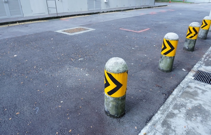
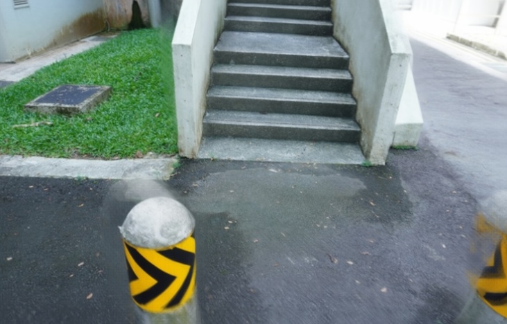
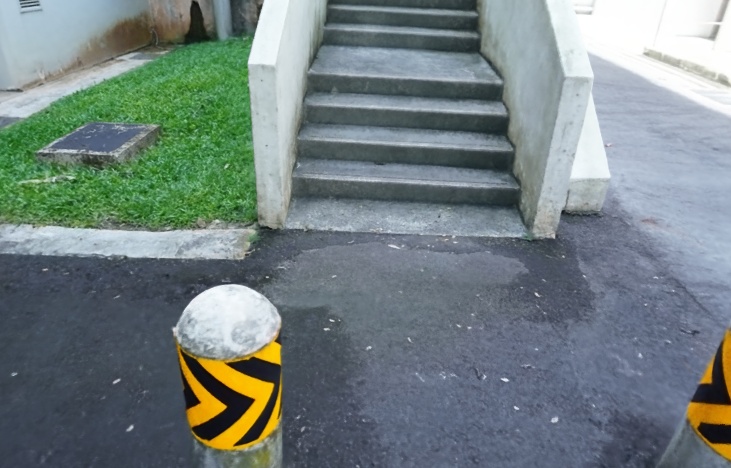
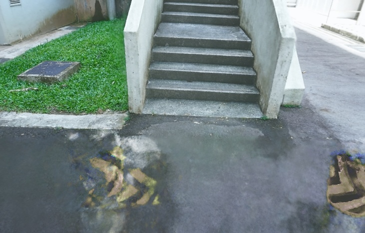
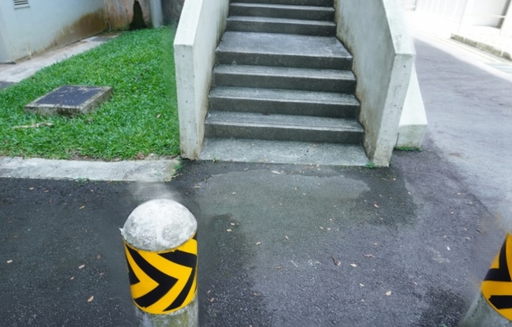
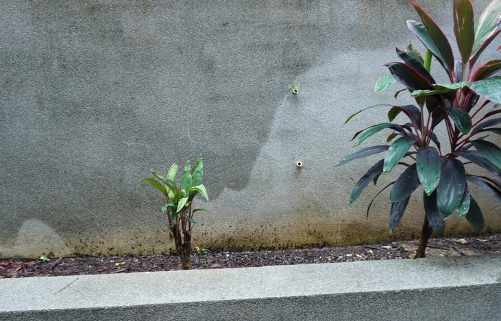
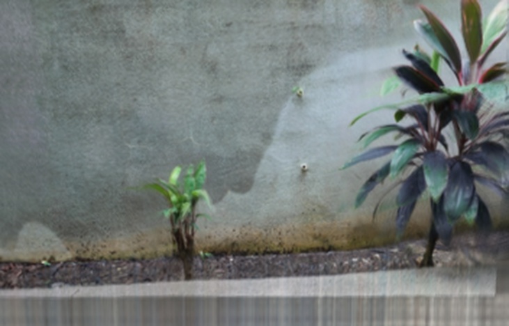
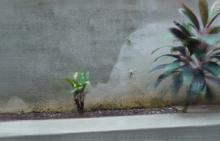
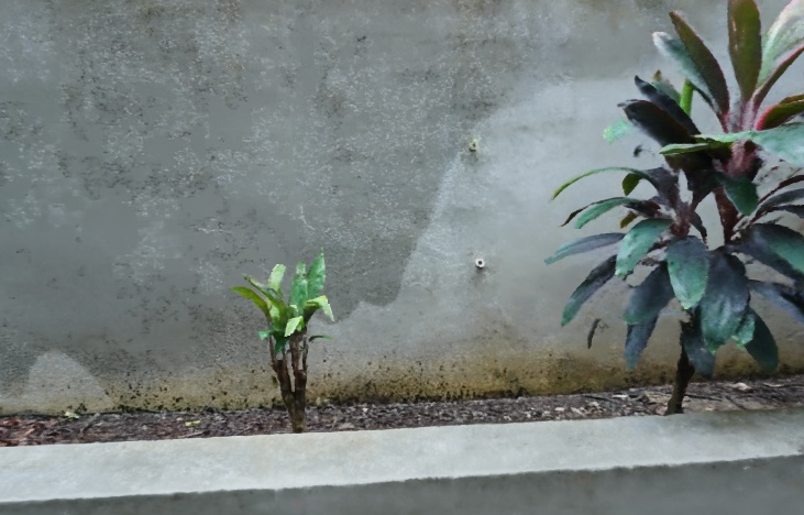
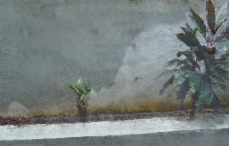
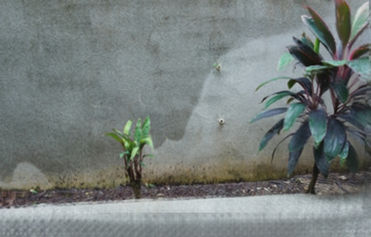
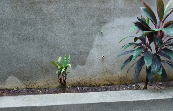
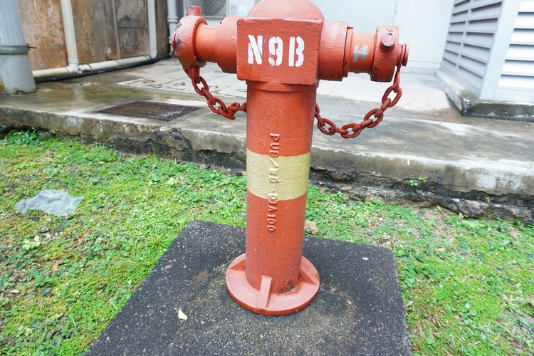
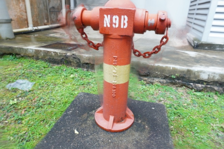
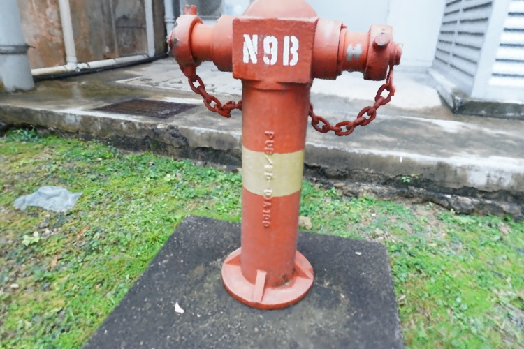
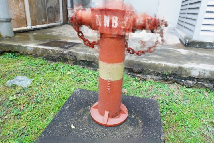
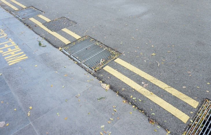
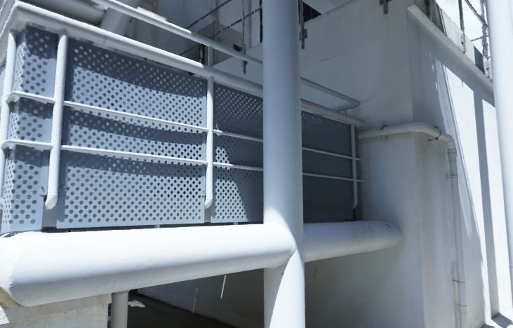
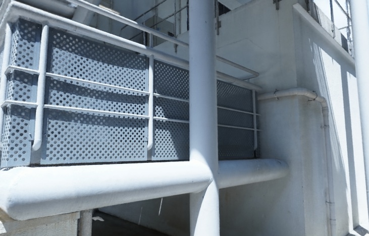
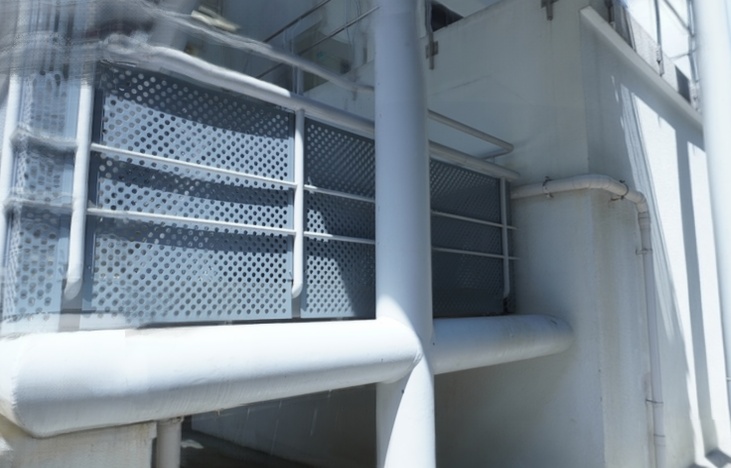
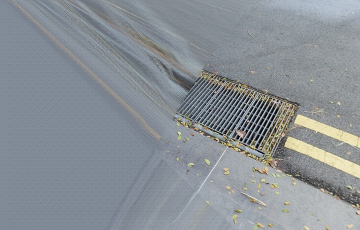
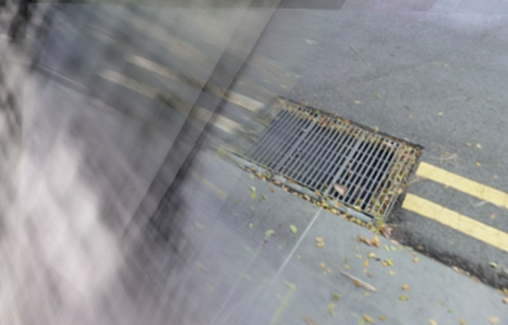
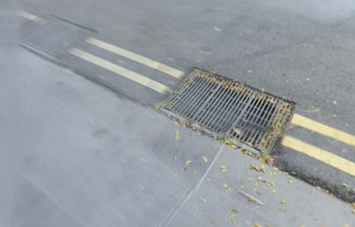
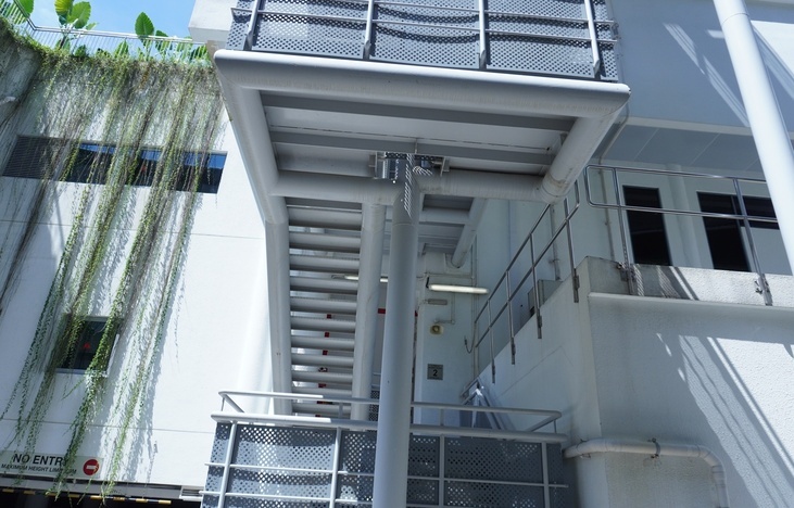
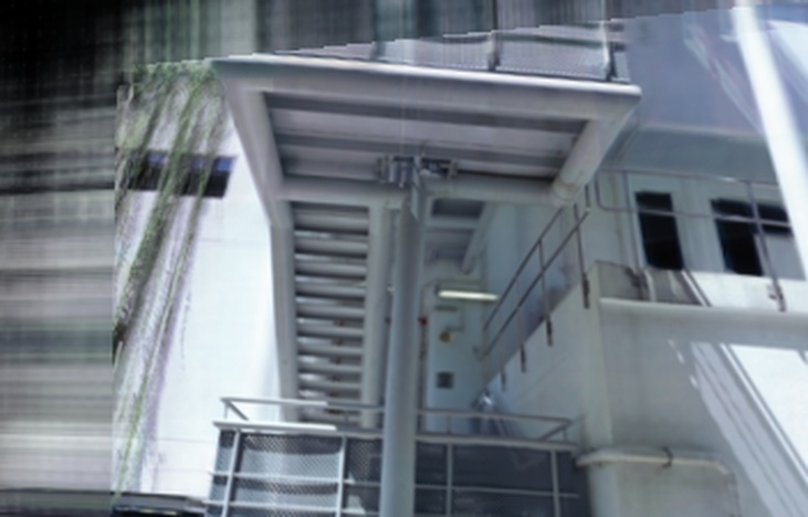
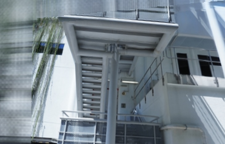
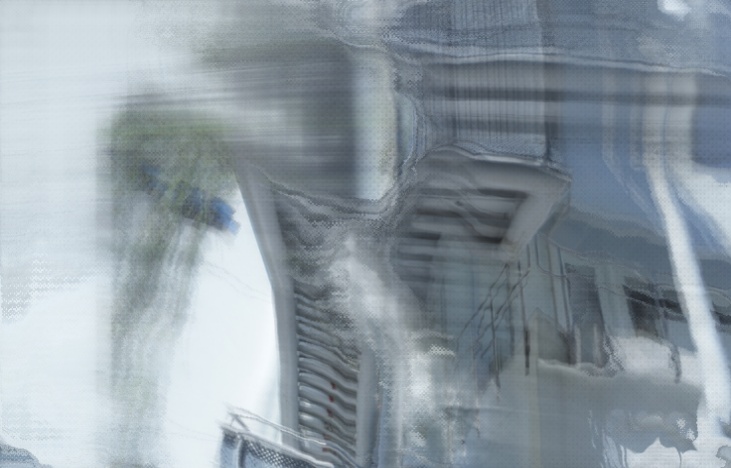
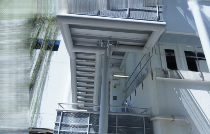
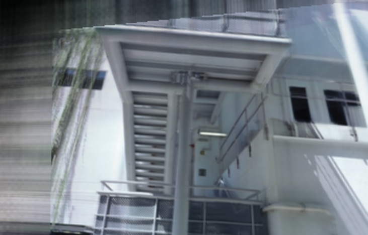
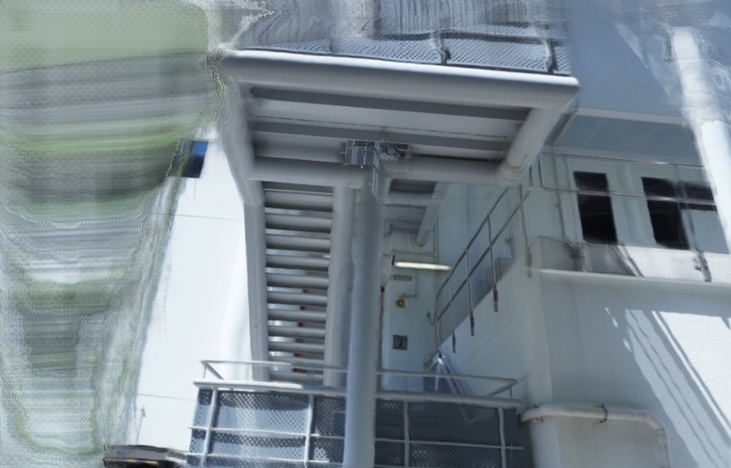
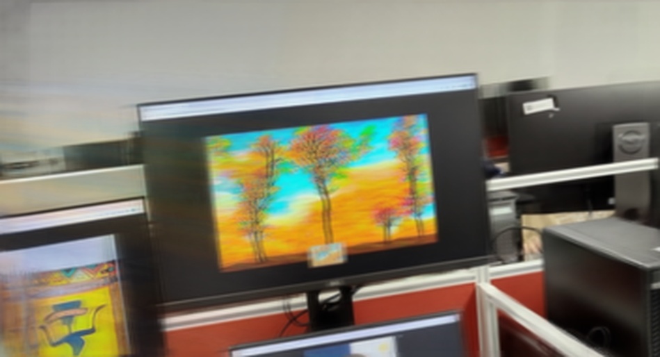
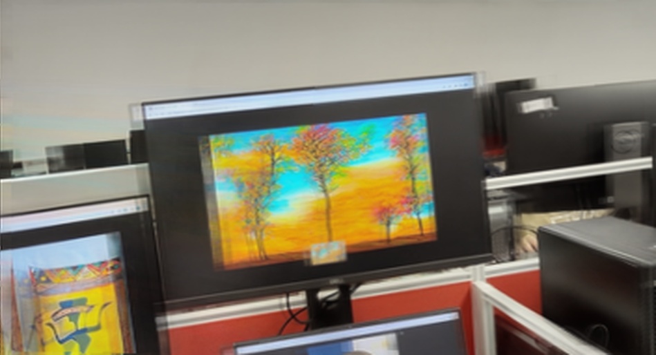
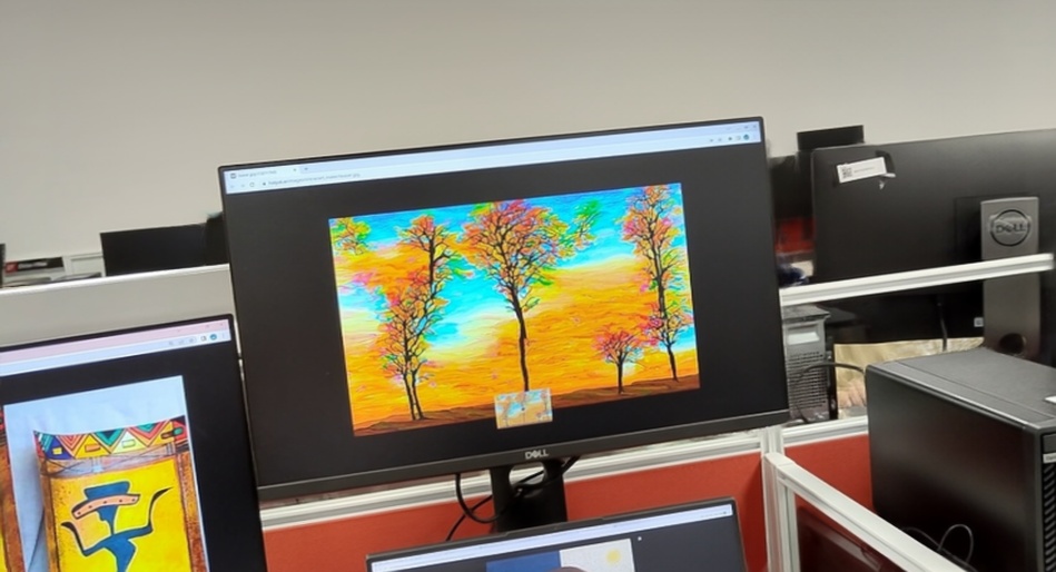
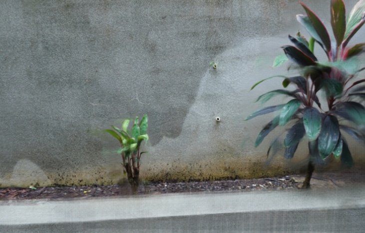
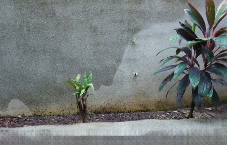
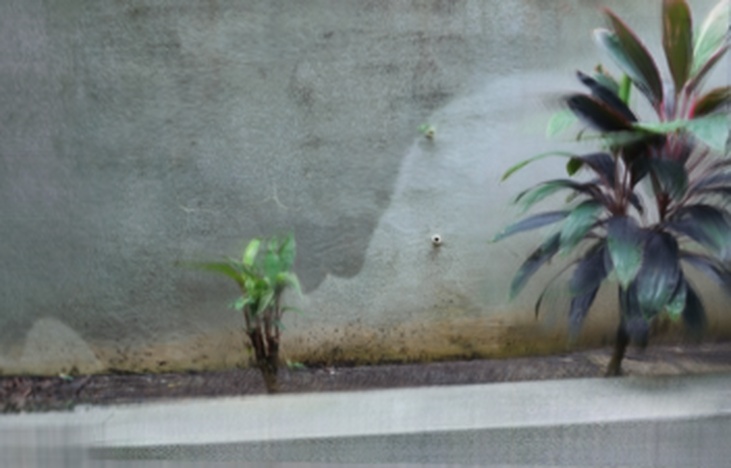
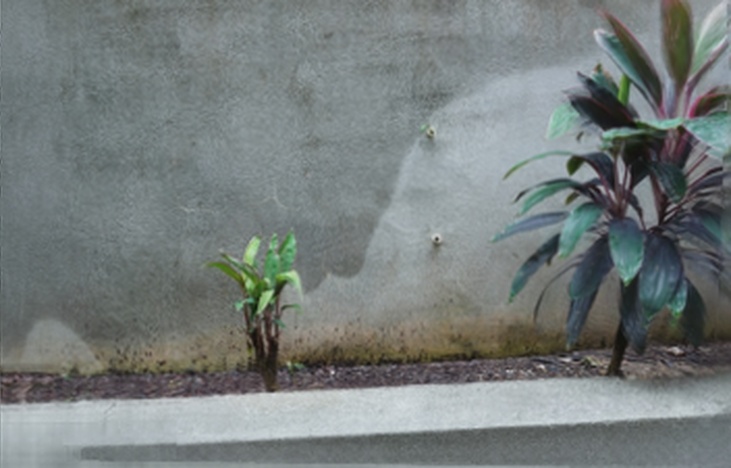
We show additional qualitative comparisons on the Free (Wang et al., 2023b) dataset in Fig. 13 and Fig. 14.

Ground truth	MVSNeRF	Ours	F2-NeRF	Zip-NeRF	MVSNeRF + ft	Ours + ft
	(Chen et al., 2021)		(Wang et al., 2023b)	(Barron et al., 2023)	(Chen et al., 2021)

Figure 13. Additional qualitative comparisons of rendering quality on the Free (Wang et al., 2023b) dataset.

Ground truth	MVSNeRF (Chen et al., 2021)	MVSNeRF + ft	ENeRF (Lin et al., 2022)	ENeRF + ft
	MVSNeRF + ours	MVSNeRF + ours + ft	ENeRF + ours	ENeRF + ours + ft
Ground truth	MVSNeRF (Chen et al., 2021)	MVSNeRF + ft	ENeRF (Lin et al., 2022)	ENeRF + ft
	MVSNeRF + ours	MVSNeRF + ours + ft	ENeRF + ours	ENeRF + ours + ft
Ground truth	MVSNeRF (Chen et al., 2021)	MVSNeRF + ft	ENeRF (Lin et al., 2022)	ENeRF + ft
	MVSNeRF + ours	MVSNeRF + ours + ft	ENeRF + ours	ENeRF + ours + ft
Ground truth	MVSNeRF (Chen et al., 2021)	MVSNeRF + ft	ENeRF (Lin et al., 2022)	ENeRF + ft
	MVSNeRF + ours	MVSNeRF + ours + ft	ENeRF + ours	ENeRF + ours + ft

Figure 14. Additional qualitative rendering quality improvements of integrating our method into MVS-based NeRF methods on the Free dataset.

F.2. ScanNet dataset

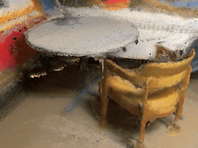
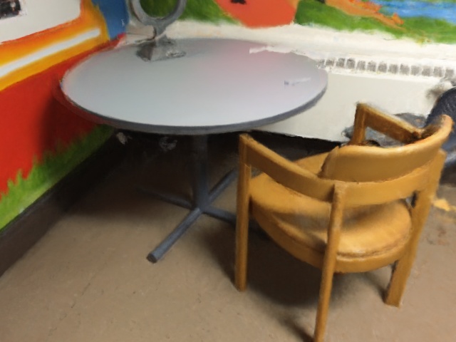
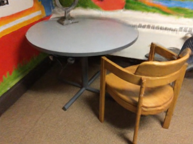
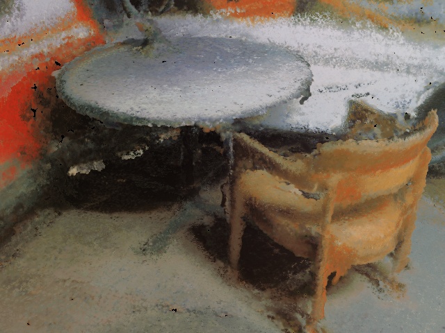
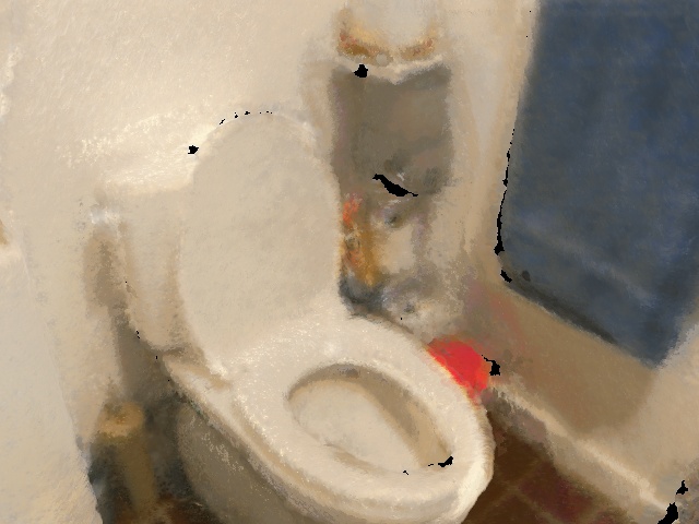
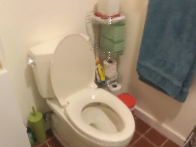
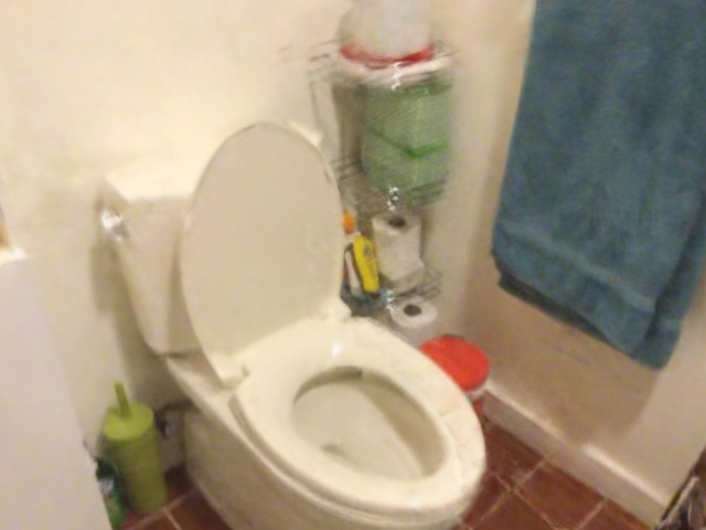
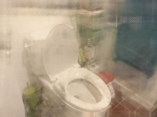
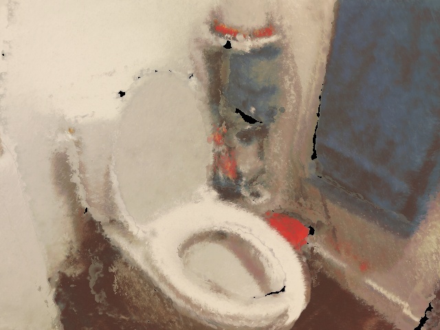
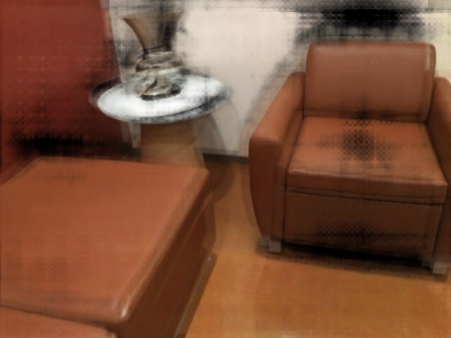
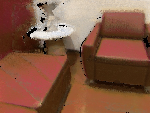
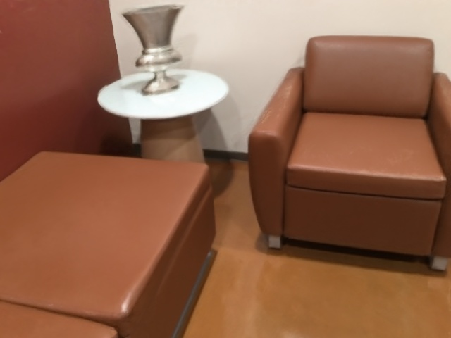
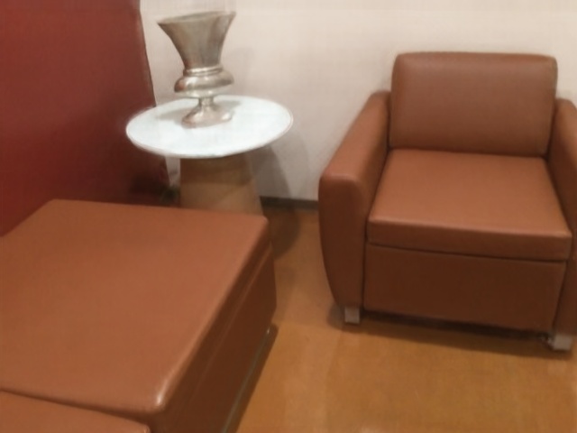
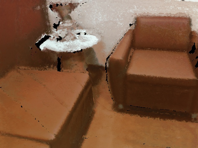
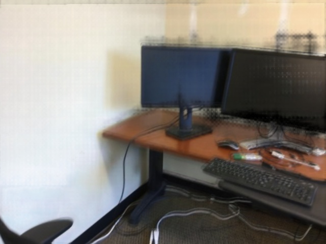
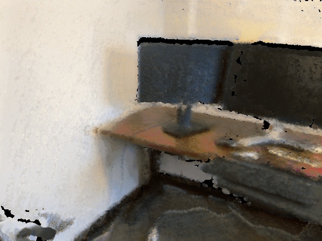
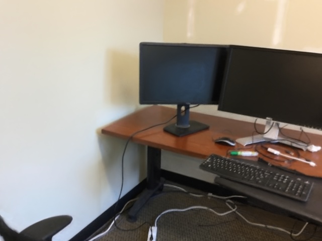
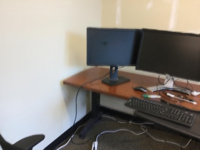
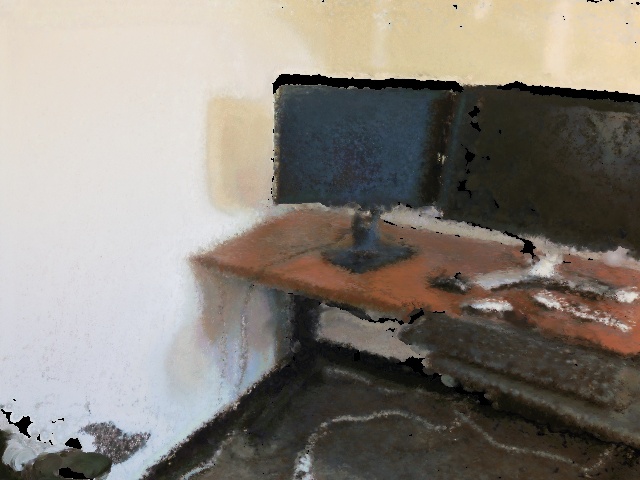
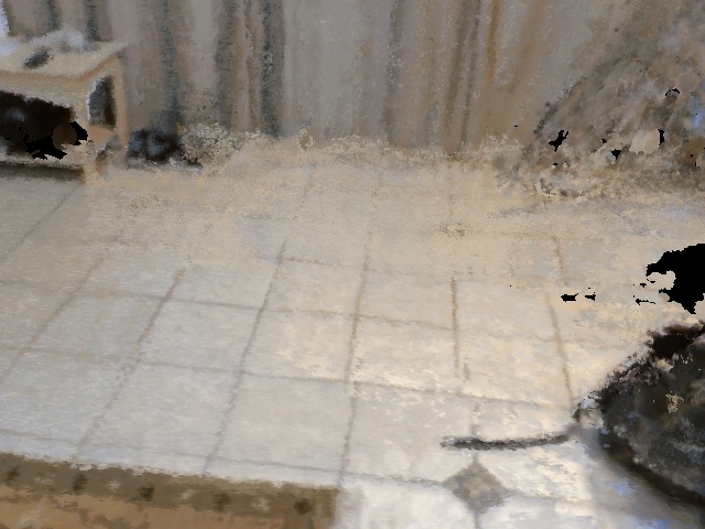
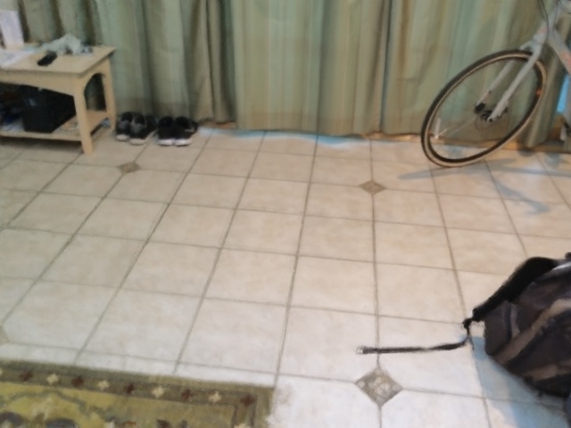
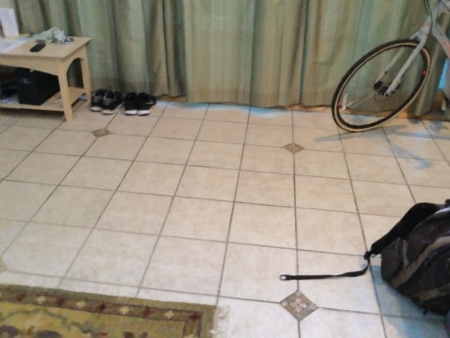
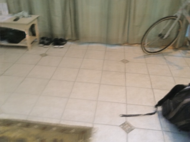
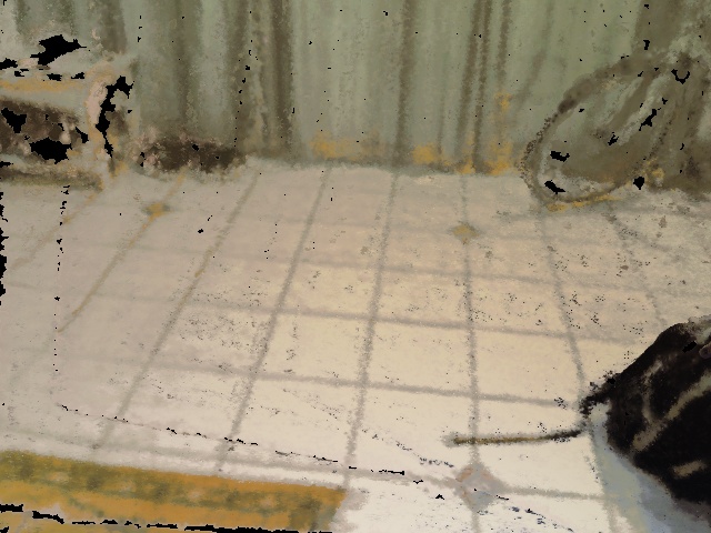
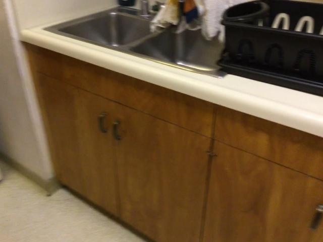
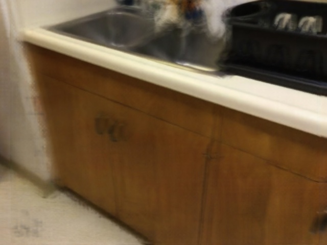
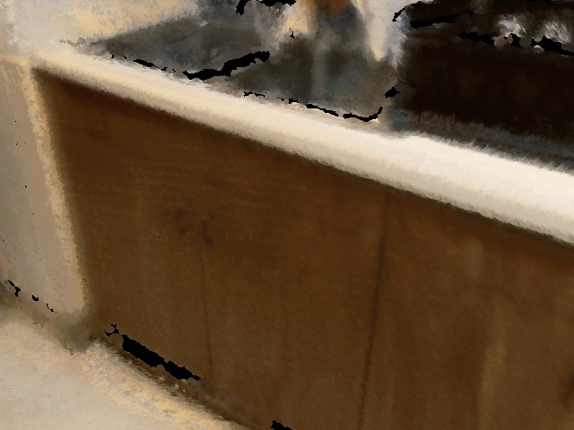
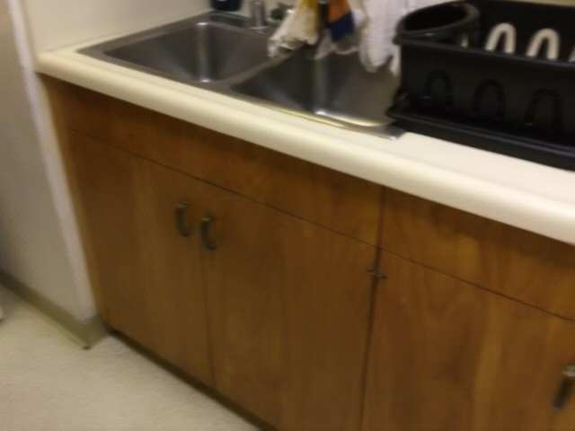
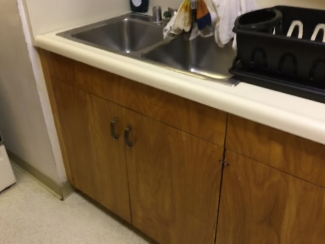
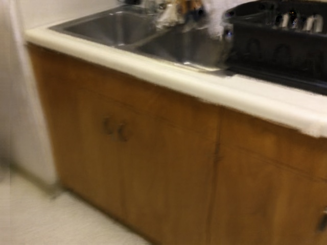
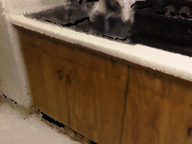
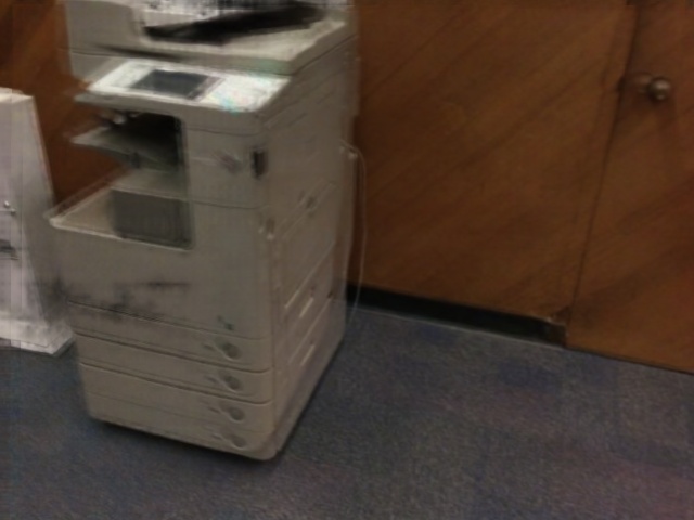
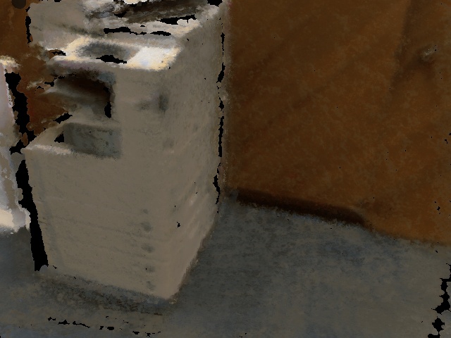
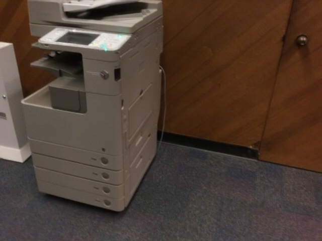
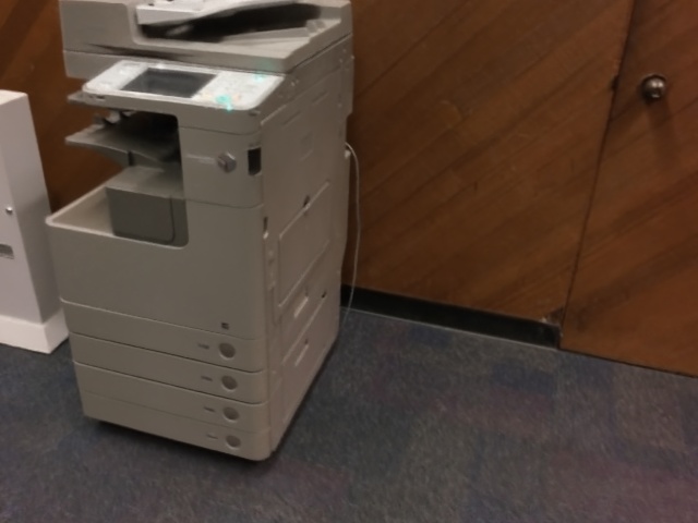
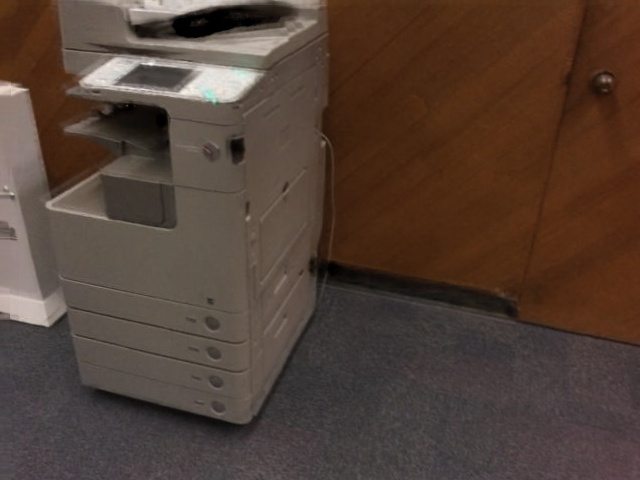
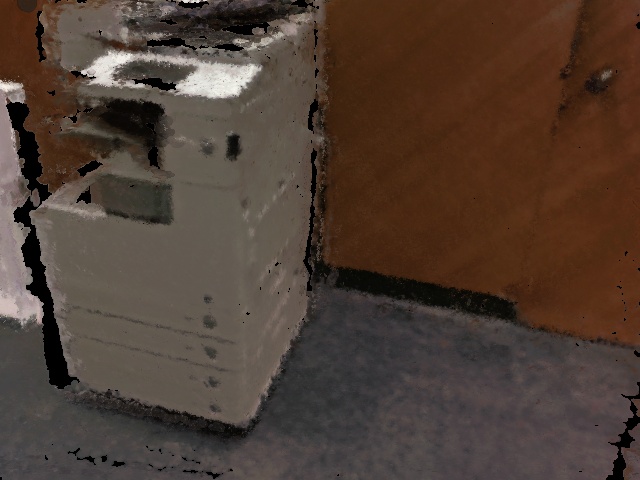
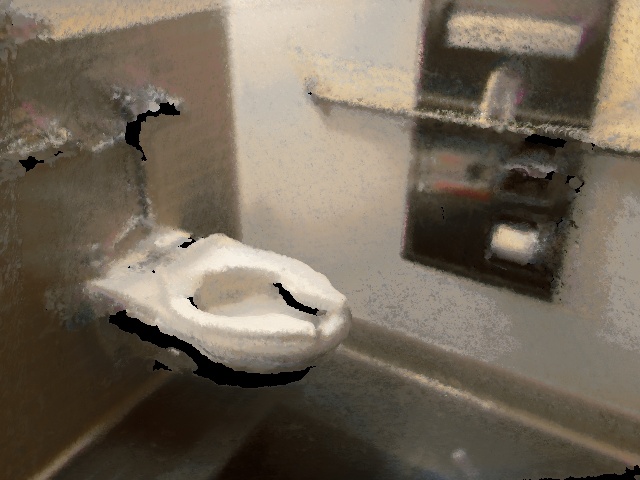
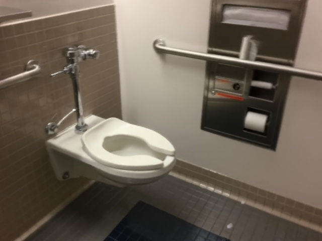
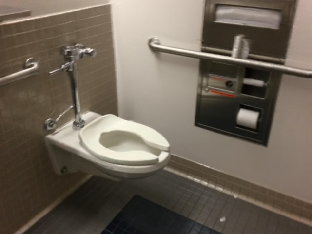
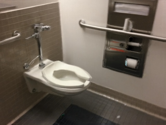
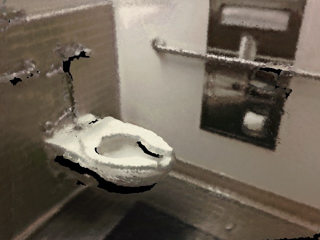
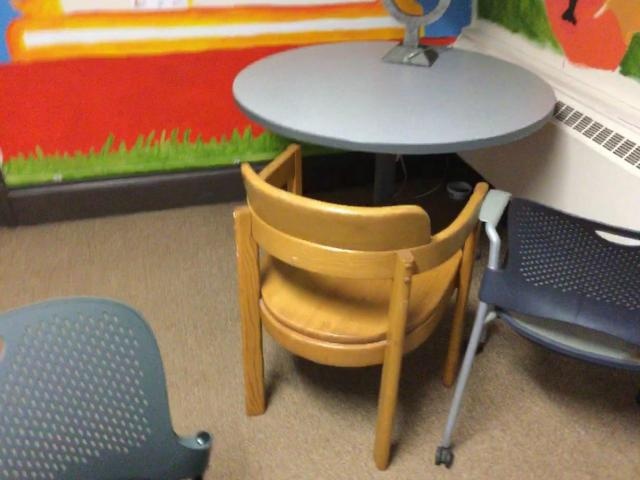
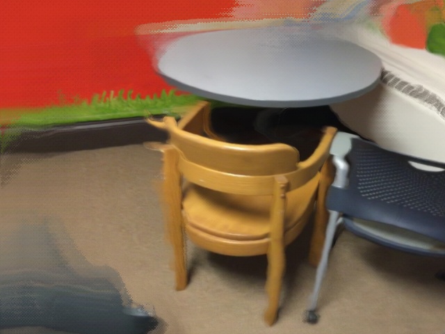
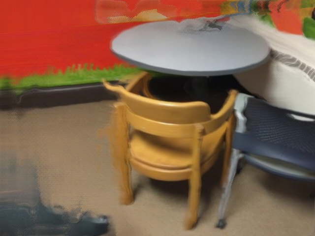
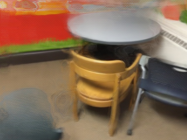
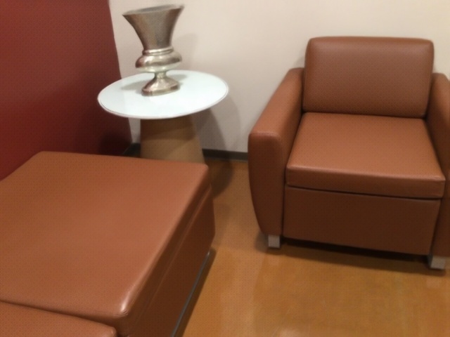
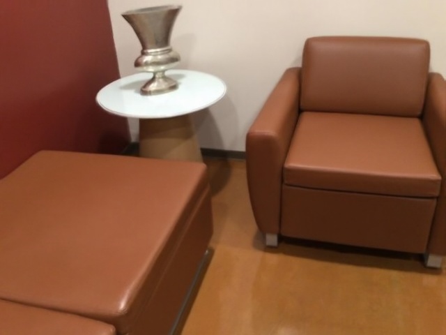
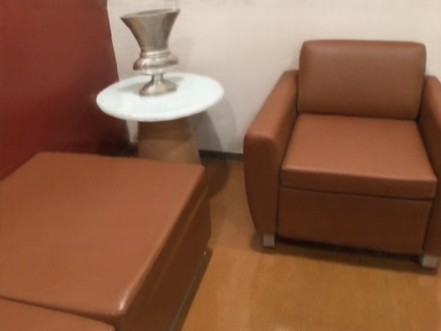
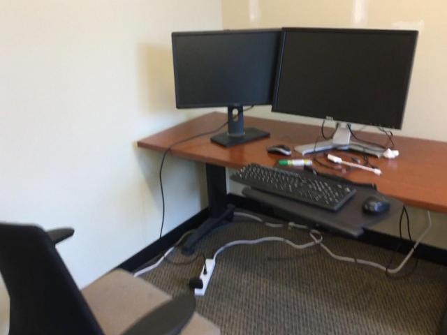
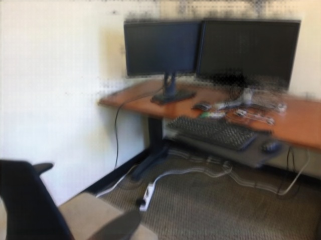
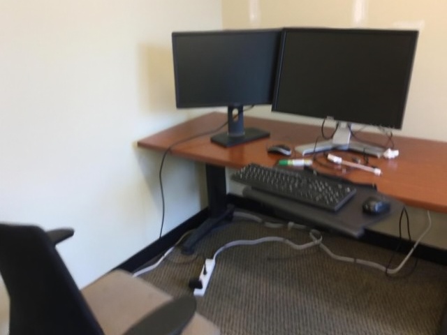
We show additional qualitative comparisons on the ScanNet (Dai et al., 2017) dataset, following the train/test split defined in NeRFusion, NerfingMVS, and SurfelNeRF, as depicted in Fig. 15 and Fig. 16.

Ground truth	MVSNeRF	SurfelNeRF	Ours	F2-NeRF	Zip-NeRF	MVSNeRF + ft	SurfelNeRF + ft	Ours + ft
	(Chen et al., 2021)	(Gao et al., 2023)		(Wang et al., 2023b)	(Barron et al., 2023)	(Chen et al., 2021)	(Gao et al., 2023)

Figure 15. Additional qualitative comparisons of rendering quality on the ScanNet (Dai et al., 2017) dataset.

Ground truth	MVSNeRF (Chen et al., 2021)	MVSNeRF + ft	ENeRF (Lin et al., 2022)	ENeRF + ft
	MVSNeRF + ours	MVSNeRF + ours + ft	ENeRF + ours	ENeRF + ours + ft
Ground truth	MVSNeRF (Chen et al., 2021)	MVSNeRF + ft	ENeRF (Lin et al., 2022)	ENeRF + ft
	MVSNeRF + ours	MVSNeRF + ours + ft	ENeRF + ours	ENeRF + ours + ft
Ground truth	MVSNeRF (Chen et al., 2021)	MVSNeRF + ft	ENeRF (Lin et al., 2022)	ENeRF + ft
	MVSNeRF + ours	MVSNeRF + ours + ft	ENeRF + ours	ENeRF + ours + ft

Figure 16. Additional qualitative rendering quality improvements of integrating our method into MVS-based NeRF methods on the ScanNet dataset.