Gyroscopic stability for nanoparticles in Stern-Gerlach Interferometry and spin contrast

Abstract

Creating macroscopic spatial quantum superposition with a nanoparticle has a multitude of applications, ranging from testing the foundations of quantum mechanics, matter-wave interferometer for detecting gravitational waves and probing the electromagnetic vacuum, dark matter detection and quantum sensors to testing the quantum nature of gravity in a lab. In this paper, we investigate the role of rotation in a matter-wave interferometer, where we show that imparting angular momentum along the direction of a defect, such as one present in the nitrogen-vacancy centre of a nanodiamond can cause an enhancement in spin contrast for a wide-ranging value of the angular momentum, e.g. $10^{3}-10^{6}$ Hz for a mass of order $10^{-14}-10^{-17}$ Kg nanodiamond. Furthermore, the imparted angular momentum can enhance the spatial superposition by almost a factor of two and possibly average out any potential permanent dipoles in the nanodiamond.

Introduction: Creating spatial superposition of nanoparticles, in particular in the context of a nitrogen-vacancy (NV) centre of nanodiamonds (ND), have ubiquitous applications, ranging from quantum metrology to quantum sensors and biology [1]. The Stern-Gerlach interferometry (SGI) [2, 3, 4] is one such method of creating the spatial superposition.

One of the critical applications of a matter-wave interferometer is in the context of testing the foundations of quantum mechanics, quantum sensors [5], detection of dark matter particles [6], gravitational waves [7]. However, a recent surge in creating designs [8, 9] for massive and large spatial superposition is to test the quantum nature of gravity in a lab [10, 11], see also [12]. The idea is to witness the entanglement between the two adjacent massive superpositions [10, 13, 14], see also [15, 16, 17, 18], which can be witnessed by reading the spin embedded in the quantum objects [10, 19, 20]. The protocol is the quantum gravity-induced entanglement of masses (QGEM). The entanglement based protocol can test short-distance Casimir and dipole entanglement mediated via photon [21, 22], extra dimensions [23], equivalence principle [14, 24], post-Newtonian gravity [25], relativistic effects in quantum electrodynamics [26], and tests beyond general relativity [27].

However, there remains a demanding requirement on quantum spatial superpositions of distinct localized states of neutral mesoscopic masses $m\sim 10^{-14}-10^{-15}$ kg over spatial separations of $\Delta x\sim{\cal O}(10-50){\rm\mu m}$ [10, 28, 29], far beyond the scales achieved to date (e.g., macromolecules $m\sim 10^{-22}$ kg over $\Delta x\sim 0.25{\rm\mu m}$, or atoms $m\sim 10^{-25}$ kg over $\Delta x\sim 0.5$ m [30, 31, 32]. However, as pointed out in [33, 34], the superposition size also depends on the nature of the spin-states of the two arms, hence on the spin-liberation degrees of freedom. The rotational effects have been known to be important in nanocrystals, see [35, 36, 37, 38, 39, 40], which severely affects the superposition size and the spin contrast [33] as discussed below.

One of the advantages of the NV spin is that an inhomogeneous magnetic field can help create a spatial superposition within SGI [8, 9, 41, 42]; besides this, the spin readout is extremely promising in the NV  [43, 44]. Hence, to finish the final spin measurement of SGI, one should combine the spatial superposition of ND and consider the coherence (or contrast) loss of the NV spin [33]. Generally speaking, there are three sources of coherence loss. The most studied coherence loss is the decoherence effect from the interaction between the ND system and the environment, such as the collisions by air molecules, electromagnetic noise, and spin-spin interaction between NV spin and another spin in the ND or the environment [10, 21, 45, 19, 28, 29, 46, 47]. Also, there is a noise in the current, such as current fluctuation which controls the magnetic field, and it’s gradient [48, 49, 50]. These decoherence effects can be mitigated by optimizing the experimental environment, such as applying higher vacuum, lower temperature, and better interaction screens for the SGI system and controlling the current in the wire. However, even if the SGI is working in an ideal environment, there is still coherence loss of the NV spin, known as the Humpty-Dumpty (H-D) effect [51, 52]. It arises from the ND’s wave packet mismatch of the two SGI arms.

In most investigations, the libration mode of an NV-centred ND has been ignored, and a challenge must be overcome to create spatial superposition via the SGI mechanism. However, for the first time, the role of libration mode has been studied recently in the context of the H-D problem, e.g. loss of spin contrast, [33, 53]. The authors pointed out that due to the NV centre’s specific Hamiltonian, the spin dynamics manifest themselves in the liberation mode. The liberation mode gives rise to two significant effects; it selects the stable state of the diamond for the two paths of the spin wave function and affects the spin contrast. In the former case, the authors showed that the stable states are $|0\rangle,|-1\rangle$ (amongst $|0\rangle,|+1\rangle,|-1\rangle$ states) for the choice of liberation mode around its minimum, e.g. the libration angle $\theta=0$. This penalises the size of the spatial superposition, and typically, the maximum superposition size becomes halved.

In Ref.[33, 53], the authors proposed a particular SGI scheme with a short interferometer duration ($t\sim 100\mu s$) and relatively small spherical object with a mass ($\sim 10^{-19}$ kg) of ND. In this case, the $\textbf{B}^{2}$ term is negligible since the ND mass is small, and more remarkably, the force acting on the centre of mass(CoM) of the ND and the torque acting on the ND can be both regarded as constants. However, none of these assumptions are correct for a more massive object. Moreover, the authors assumed that the initial angular momentum of the nanodiamond is vanishingly tiny; it is possible to initiate the system to its motional ground state, such that the angular momentum in all three directions in the lab frame is within the uncertainty principle. However, this paper will give a new twist to this libration mode. Instead of treating it as a problem, we will provide a unique mechanism to mitigate the spin contrast while maintaining the superposition size governed by both $|+1\rangle,|-1\rangle$ states, as shown in an inhomogeneous magnetic field, see [42], for a heavy ND of mass such as $10^{-14}-10^{-17}$ kg, where we also include the effect of diamagnetic induced potential in the Hamiltonian.

The critical result of this paper can be summarised as such; we will demonstrate that if we had initiated the nanodiamond with an initial angular momentum along the direction of the spatial superposition, we would be able to use both $|+1\rangle,|-1\rangle$ spin states, which would favour the size of the superposition. More importantly, an initial angular momentum will aid in obtaining a better spin contrast. Furthermore, having a considerable initial angular momentum can also help us average any deleterious effect due to permanent dipoles, as shown in [54, 55]. In the latter case, the authors observed that dipole effects are mitigated while rotating the nanoparticle.

Hamiltonian: The Hamiltonian of a levitated ND with a single spin-1 NV centre can be recast as [41, 42, 33]:

$$H=\frac{\textbf{p}^{2}}{2m}+\sum_{j=1}^{3}\frac{L^{2}_{j}}{2I_{j}}+\frac{-\chi_{\rho}m}{2\mu_{0}}\textbf{B}^{2}+\mu\,\textbf{s}\cdot\textbf{B}+DS_{\parallel}^{2}\,,$$ (1)

where $m$ and $I_{j}$ are the mass and inertia moments of the ND respectively, $\chi_{\rho}=-6.2\times 10^{-9}m^{3}/kg$ represent the mass magnetic susceptibility of diamonds, the magnetic moment of the NV is $\mu=e\hbar/2m_{e}=h\times 2.8{\rm MHz/G}$, and $D=h\times 2.87{\rm GHz}$ is the zero-field splitting of the NV centre, $h=6.62607015\times 10^{-34}{\rm JHz^{-1}}$, $S_{\parallel}=\textbf{s}\cdot\hat{n}_{s}$ is the projection of the NV spin on the NV crystalline direction, denoted as $\hat{n}_{s}$. The $D$ term is the zero-point splitting term, non-vanishing for $s>1/2$ spin systems.

Illustrative model of spatial superposition: To emulate all the terms in the Hamiltonian 1, we will follow the SGI scheme proposed in[42], where the following time-varying spatial magnetic field is applied as a part of the SGI setup:

$$\vec{B}(z,x)=\left\{\begin{aligned} &(B_{0}-\eta z)\hat{z}+\eta x\hat{x}\,,\qquad t<\tau_{1}\\ &\qquad\qquad B_{1}\hat{z}\,,\qquad\quad\quad\tau_{1}\leq t<\tau_{2}\\ &-(B_{0}-\eta z)\hat{z}-\eta x\hat{x}\,,\quad t>\tau_{2}\end{aligned}\right.$$ (2)

in which $B_{0}$, $B_{1}$ and $\eta$ are constant. In [42], initially, the ND is set as translationally and rotationally static at the original point $z=0$ and $x=0$. Meanwhile, the NV axis $\hat{n}_{s}$ is oriented to the $\hat{z}$ direction. Then, we choose the NV axis as our quantization orientation of the NV spin state, and the spin state is initially set as $s=0$ state. At $t=0$, a $\pi/2$ pulse is applied to prepare the superposition state $|s\rangle=(\lvert+1\rangle+\lvert-1\rangle)/\sqrt{2}$ of the NV spin. In Ref.[42], the rotation of ND is not considered so that the NV axis is assumed always oriented to $\hat{z}$ direction. Besides, since $x=0$ is the equilibrium position of the harmonic potential of $\hat{x}$ direction, the translational motion along $\hat{x}$ axis is always static except for initial thermal noise, which can be reduced by cooling the initial vibration of the ND [56, 57, 58]. This can be arranged in a narrow trap where the motion is restricted to effectively one dimension; see [28]. Therefore, the motion along $\hat{x}$ direction is assumed negligible. The homogeneous magnetic field $B_{1}\hat{z}$ set during $\tau_{1}$ to $\tau_{2}$ aims to ensure that the ND is always in enough sizeable magnetic field to avoid Majorana spin flipping [42]. During $\tau_{1}\leq t<\tau_{2}$, the NV-spin is mapped to the nuclear spin; effectively, the diamagnetic term dictates the dynamics of the ND. Based on the above initial conditions and assumptions, we realize a 1-dimensional SGI, where only the motion along $\hat{z}$ axis should be considered. Then, from the Hamiltonian Eq. (1) and the magnetic field Eq. (2), we obtain the effective Hamiltonian for the motion of ND in the $z$ direction:

$$H_{z}=\frac{\hat{p}_{z}^{2}}{2m}+\frac{1}{2}m\Omega^{2}(\hat{z}-Z_{0})^{2}-\tilde{\eta}(t)\mu\hat{s}(\hat{z}-Z_{0})\,.$$ (3)

in which $\Omega$ and $Z_{0}$ is defined as $\Omega^{2}=-\chi_{\rho}\tilde{\eta}^{2}/\mu_{0}$, $Z_{0}=B_{0}/\eta$, and $\tilde{\eta}(t)$ is the magnetic field gradient, namely $\tilde{\eta}(t)=-\eta,~{}0,~{}+\eta$ when $t<\tau_{1}$, $\tau_{1}\leq t<\tau_{2}$, and $t\geq\tau_{2}$ respectively. As we can see, the ND is in a spatial harmonic potential when the linearized magnetic field is applied, and the equilibrium position of the harmonic potential depends on the NV spin state, e.g. the last term $\hat{s}$ of Eq. 3. The largest spatial size of superposition during the SGI interferometer can be estimated by the distance between the equilibrium position of $s=\pm 1$ state, namely $\Delta z\approx 2\mu\eta/m\Omega^{2}=2\mu_{0}\mu/(-\chi_{\rho}m\eta)$ [41, 42], which is inversely proportional to magnetic field gradient $\eta$ and the mass $m$ of ND. The time scale of the interferometer is about $\Omega\propto\eta^{-1}$. To close the two SGI arms, a rapid microwave pulse should flip the NV spin state at an appropriate time $\tau_{3}$. Afterwards, the interferometer is closed at a specific time, denoted as $\tau_{4}$.

Rotational Dynamics: Let us investigate how the rotational dynamics of ND affect the SGI model. Remarkably, since the $s=+1$ state is unstable[33, 53], the ND with $s=+1$ spin state will have a significant rotation, so the NV spin is no longer orientated to the $\hat{z}$ axis, Then the spatial trajectory will be changed a lot. To cure this issue, a possible way is creating spatial superposition by $|s\rangle=(\lvert 0\rangle+\lvert-1\rangle)/\sqrt{2}$, because the ND with $s=0$ state is torque-free and with $s=-1$ state is rotationally stable [33, 53]. This novel approach ensures that the NV spin is always approximately orientated to the $\hat{z}$ axis; however, the price is that the superposition size is halved, and to make matters worse, the spin contrast is almost zero because of the mismatch between the two SGI angular paths and the mismatch of the quantum uncertainty of the two asymmetric angular wave packet(see appendix.A). To reduce the contrast loss, schemes using $|s\rangle=(\lvert 0\rangle+\lvert-1\rangle)/\sqrt{2}$ state require extreme constraints for the location of NV spin in the ND, e.g. within nanometer separation distance of the NV centre from the centre of mass (CoM) of the ND, and very difficult fine-tuning of experimental parameters, see [33].

Figure 1: The ND sphere model and the three Euler angles $\{\phi,\theta,\psi\}$ in the ZXZ convention. We take the gauge that $\{\hat{n}_{1},\hat{n}_{2},\hat{n}_{3}\}$ are coincide with $\{x,y,z\}$ respectively when $\phi=\theta=\psi=0$. $\vec{d}$ represents the vector of the location of the NV spin, and the angle between $\hat{n}_{3}$ and $\vec{d}$ is labelled as $\alpha$. The external magnetic field is aligned along the $z$ and $x$-axis. However, we assume that the superposition is one dimensional and it will be created solely along the $z$-axis; we set $x=0$ always. Our new proposition to mitigate the loss of spin contrast is that the ND is initially spinning around $\hat{n}_{3}$-axis with frequency $\omega_{0}$.

New proposition: We propose the following scheme to alleviate the fine-tuning of parameters for the spin contrast loss in the SGI setup. The key is giving the ND a sufficient initial angular momentum that points to the NV axis. The model we built is shown in Fig.1, where the ND is considered a nano-sphere, namely $I_{1}=I_{2}=I_{3}=I$. We can easily generalise this to cylinder, but we will keep it simple in this paper and pursue with a spherical assumption. The rotational motion is described by three Euler angles: the procession angle $\phi$, the nutation angle $\theta$, and the rotation angle $\psi$. We study the general case of the NV centre not being located at the centre of mass (COM) of the ND. Initially, we levitate an ND sphere and use circularly polarized light to rotate the ND with angular velocity $\omega_{0}$ around the $\hat{n}_{3}$ axis, experimentally feasible, see [39]. Then, the NV spin state is prepared as the superposition state $|s\rangle=(\lvert+1\rangle+\lvert-1\rangle)/\sqrt{2}$. The next step is turning on the magnetic field $\vec{B}(z,x)$ at $t=0$, where the $\hat{z}$ direction should be as coincides with the initial ND rotation axis $\hat{n}_{3}$ as possible. Our experimental setup can tolerate a slight initial angle $\theta_{0}$ between $\hat{n}_{3}$ and $\hat{z}$.

Thanks to the gyroscopic effect, the rotation axis of the fast-spinning ND is now stable, which means that the orientation of $\hat{n}_{3}$ and $\hat{n}_{s}$ can always be approximately aligned with the $\hat{z}$ axis. Therefore, in this case, when considering the spatial trajectory of the two arms of SGI, one can safely assume that the NV spin orientation is always keeping parallel to the magnetic direction $\hat{z}$. Furthermore, we should ensure the NV state $s=\pm 1$ is stable during the SGI. However, some special values of rotation frequency $\omega_{0}$ possibly lead to the spin resonant transition $s=\pm 1\leftrightarrow 0$. To maintain the spin state during the SGI, the ND rotation frequency should satisfy the off-resonant condition $\omega_{0}\ll(D\pm\mu B)/\hbar\sim$ GHz (see [40, 38] and appendix.B). Thus, the spatial trajectories of the SGI model do not change significantly due to the rotational dynamics of the ND. The time evolution of the two arms spatial trajectories is shown in appendix.A.

Rotational dynamics: To describe the rotational dynamics, we define the rotational Lagrangian $\mathcal{L}=T-V$, where the rotational kinetic energy $T$ of the ND sphere in terms of Euler angles is given by [33, 53]

$$T=\frac{I}{2}(\dot{\theta}^{2}+\dot{\phi}^{2}{\rm sin}^{2}\theta)+\frac{I}{2}(\dot{\phi}{\rm cos}\theta+\dot{\psi})^{2}\,,$$ (4)

and the potential term, $V$, generates torque acting on ND’s rotation. The NV spin vector is assumed to be fixed in the NV axis direction, namely $\textbf{s}=s\hat{n}_{s}$. Therefore, the mechanical rotation of the ND will rotate the NV spin magnetic moment, $\mu\textbf{s}$, and spin angular momentum, S, which implies that the NV spin causes two torques for the rotation of ND. The first torque is casued by the Zeeman term: $\mu\textbf{s}\cdot\textbf{B}=\mu s\,\hat{n}_{s}\cdot\textbf{B}$. Another torque is from the time-dependent rotation of the spin angular momentum: S, namely $\textbf{M}\equiv d\textbf{S}/dt=\boldsymbol{\omega}_{0}\times\textbf{S}=\textbf{S}\times\textbf{L}/I$, which is known as Einstein-de Haas(EdH) effect [59, 60, 61]. The effect is equivalent to adding a spin-rotational coupling term $\textbf{S}\cdot\textbf{L}/I$ in the potential $V$, which leads to the additional torque $[L_{i},S_{j}L_{j}/I]=i\varepsilon_{ijk}S_{j}L_{k}/I$ to the angular momentum evolution $\propto\dot{L_{i}}$. It means that the NV spin can still affect the nano particle’s rotation to some extent even when $\textbf{B}=0$ via the EdH effect [38]. Therefore, including the Zeeman term and EdH term, the potential term $V$ can be written as

$$V=\textbf{s}\cdot(\mu\textbf{B}+\hbar\frac{\textbf{L}}{I})\,.$$ (5)

In this paper, for simplicity, we wish to work in a regime where the effect of EdH term $\textbf{S}\cdot\textbf{L}/I$ is negligible in the potential, e.g. $\hbar L/I=\hbar\omega_{0}\ll\mu B$. This will be the first constraint on $\omega_{0}$. Moreover, the condition $\hbar\omega_{0}\ll\mu B$ implies that the rotational frequency $\omega_{0}$ of the magnetic field in the diamond frame is much smaller than the Larmor precession frequency $eB/m_{e}=2\mu B/\hbar$ of the NV electron spin. It ensures an almost zero probability of Majorana flipping of the NV spin [42].

Therefore, in the $V$ term, the Zeeman term $\mu sB{\rm cos}\theta$ is important for our dynamics, independent of the angular momentum variables. Then, we can define the canonical momentum of the three Euler angles

$$p_{\theta} \equiv \partial\mathcal{L}/\partial\dot{\theta}=I\dot{\theta}\,,$$

$$p_{\phi} \equiv \partial\mathcal{L}/\partial\dot{\phi}=I(\dot{\phi}+\dot{\psi}\,{\rm cos}\theta)=L_{z}\,,$$ (6)

$$p_{\psi} \equiv \partial\mathcal{L}/\partial\dot{\psi}=I(\dot{\psi}+\dot{\phi}\,{\rm cos}\theta)=L_{3}\,.$$

Then, the Hamiltonian for ND’s rotational evolution is

$$H_{r}=\frac{p_{\theta}^{2}}{2I}+\frac{p_{\psi}^{2}}{2I}+\frac{(p_{\phi}-p_{\psi}{\rm cos}\theta)^{2}}{2I\,{\rm sin}^{2}\theta}+\mu sB_{nv}{\rm cos}\theta\,,$$ (7)

where $B_{nv}=B_{c}+\tilde{\eta}(t)d\,({\rm cos}\alpha\,{\rm cos}\theta+{\rm sin}\theta\,{\rm sin}\alpha\,{\rm cos}\psi)$ denotes the magnetic field strength at the location of the NV centre, and $B_{c}$ is the magnetic field strength at the COM. Since the gradient in the magnetic field, $\eta d\ll B_{c}$, we assume that $B_{nv}\approx B_{c}$ for our analysis. Therefore, the canonical momentum $p_{\psi}$ and $p_{\phi}$ are conserved (e.g. no external magnetic force is acting along these directions):

$$p_{\phi}=I\omega_{0}{\rm cos}\theta_{0}\,,\quad p_{\psi}=I\omega_{0}\,.$$ (8)

Substituting the conserved quantities Eq. (8) to Eq. (7), we obtain the Hamiltonian for the evolution of $\theta$, and then, taking the small oscillation approximation $\theta-\theta_{0}\ll\theta_{0}\ll 1$, we end up with the equation of motion of, $\theta$, as follows:

$$\ddot{\theta}=-\left(\omega_{0}^{2}-\frac{\mu sB_{c}(t)}{I}\right)(\theta-\theta_{0})+\frac{\mu s}{I}B_{c}(t)\theta_{0}\,,$$ (9)

The above Eq.(9) implies that the orientation of NV axis is stable for both $s=+1$ and $s=-1$ spin state as long as the requirement $\omega_{0}^{2}>\mu B_{c}/I$ is satisfied. Further, to ensure a small oscillation condition of $\theta$, we need $\omega_{0}^{2}\gg\mu B_{c}/I$. Based on the above discussions, we can conclude the order of magnitude for parameters in the SGI experimental setup as follows:

$$\sqrt{\frac{\mu B_{c}}{I}}\ll\omega_{0}\ll\frac{\mu B_{c}}{\hbar}\,,\ {\rm and}\ \omega_{0}\ll\frac{D\pm\mu B_{c}}{\hbar}\,.$$ (10)

For the experimental parameters set in Fig.2, the order of magnitude of $\sqrt{\mu B_{c}/I}$ is about $2\pi\times 10^{2}{\rm Hz}$, $\mu B_{c}/\hbar\sim 5-300{\rm MHz}$, and $D/\hbar=2\pi\times 2.87$GHz. So the value of $\omega_{0}$ can be set in the order of $\omega_{0}\sim{\rm kHz}-{\rm MHz}$.

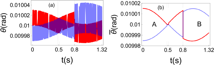
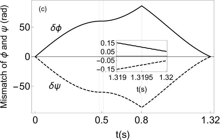
Figure 2: Subfigure (a) The red and blue trajectories represent the numerical time evolution of nutation mode $\theta(t)$ for the two SGI arms. Subfigure (b), we show The equilibrium position $\bar{\theta}(t)$ of the oscillation mode $\theta(t)$. (c) shows the evolution of the procession angle difference $\delta\phi(t)$ and rotation angle difference $\delta\psi(t)$ between the two SGI arms. In this plot, we set $m=10^{-17}$kg, $B_{0}=100G$, $B_{1}=1.0G$, $\eta=0.45G/\mu m$. Note that following [42], there are four time stages, they are $\tau_{1}=0.482s$, $\tau_{2}=0.514s$, $\theta_{0}=0.01$, $\omega_{0}=2\pi\times 10{\rm kHz}$, $d=10{\rm nm}$, $\alpha=\pi/6$. We reverse the NV spin state between $\lvert+1\rangle$ and $\lvert-1\rangle$ at $\tau_{3}=0.8022s$. The spatial trajectory of the two SGI arms closed at $\tau_{4}=1.320s$. Vertical lines show these time stages here, except $\tau_{4}=1.32s$.

For SGI models with long duration, the variation of $B_{c}$ in Eq. (9) is slow compared with the fast oscillation of $\theta$. So the nutation mode $\theta(t)$ shows a fast harmonic oscillation with frequency $\omega=\sqrt{\omega_{0}^{2}-\mu sB_{c}/I}\approx\omega_{0}$ and adiabatically evolving equilibrium position $\bar{\theta}(t)$, illustrated in Fig.2, where $\bar{\theta}$ is obtained from Eq. (9) as (see appendix.C for the derivation):

$$\bar{\theta}(t)\approx\theta_{0}+\frac{\mu s}{I\omega_{0}^{2}}B_{c}(t)\theta_{0}\,.$$ (11)

Here, we take the ground state of the harmonic trap as the initial state of nutation mode, i.e. $\theta(0)=\theta_{0}$ and $\dot{\theta}=0$. The amplitude of the nutation mode $\theta(t)$ can be estimated as $A_{\theta}(0)=\mu B_{0}\theta_{0}/I\omega_{0}^{2}$ during $0\leq t<\tau_{3}$. At $t=\tau_{3}$, the NV spin is flipped, then the equilibrium position $\bar{\theta}$ changes rapidly, disturbs the oscillation, and the nutation amplitude is somewhat enhanced. Nevertheless, the final nutation amplitudes of the two SGI arms are still on the same order of magnitude of $\mu B_{0}\theta_{0}/I\omega_{0}^{2}$ therefore, the final mismatch of $\theta$, denoted as $\delta\theta$, should be on the same order as well. More precisely, the maximum of $\delta\theta$ can be estimated by (see appendix.C)

$$\delta\theta(\tau_{4})\lesssim\frac{8\mu B_{0}\theta_{0}}{I\omega_{0}^{2}}\,.$$ (12)

The mismatch of nutation angle $\theta$ is inevitable, but it can be highly reduced by an immense value of $\omega_{0}$ and a small value of $\theta_{0}$. For the case of $\omega_{0}=10$kHz, $\theta_{0}=0.01$ and $B_{0}=100$G, the mismatch of $\theta$ in on the order of $10^{-5}$, incredibly small.

For the precession $\phi(t)$ and the rotation mode $\psi(t)$, according to Eq. (Gyroscopic stability for nanoparticles in Stern-Gerlach Interferometry and spin contrast) and (8), the equations of motion are

$$\dot{\phi} =\frac{\omega_{0}}{{\rm sin}^{2}\theta_{0}}({\rm cos}\theta_{0}-{\rm cos}\theta)\approx\frac{\omega_{0}}{\theta_{0}}(\theta-\theta_{0})\,,$$ (13)

$$\dot{\psi} =\frac{\omega_{0}}{{\rm sin}^{2}\theta_{0}}(1-{\rm cos}\theta_{0}{\rm cos}\theta)\approx-\frac{\omega_{0}}{\theta_{0}}(\theta-\theta_{0})\,,$$ (14)

where we use the condition $\theta-\theta_{0}\ll\theta_{0}\ll 1$ Rad for our setup (a small angle approximation for $\theta$). The mismatch of classical trajectory of $\phi(t)$ is given by

$$\delta\phi(\tau_{4})\approx\frac{\omega_{0}}{\theta_{0}}\int_{0}^{\tau_{4}}dt\,(\bar{\theta}_{L}-\bar{\theta}_{R})=\frac{\omega_{0}}{\theta_{0}}(\Sigma_{A}-\Sigma_{B})\,,$$ (15)

where $\bar{\theta}_{L}$ and $\bar{\theta}_{R}$ represent the red and blue curves shown in Fig.2(b), and $\Sigma_{A}$ and $\Sigma_{B}$ labels the area of the region $A$ and $B$ respectively. The mismatch of $\psi$ is given by $\delta\psi=-\delta\phi$.

Generally, the area $\Sigma_{A}$ and $\Sigma_{B}$ are inequal. But, one can regulate the trajectory of $\bar{\theta}(t)$ by optimizing the experimental parameters, such as $B_{1}$ and $B_{0}$, to make $\Sigma_{A}\approx\Sigma_{B}$. For example, as illustrated in Fig.2(c), the parameters used in Fig. 2 result in a almost vanish mismatch of $\phi$ and $\psi$, in which $|\delta\phi|=|\delta\psi|\approx 0.05$. Remarkably, from the equation (11,15), we have $\delta\phi\propto\omega_{0}^{-1}$. So, the mismatch $\delta\phi$ and $\delta\psi$ can be further reduced by applying a larger $\omega_{0}$, namely $|\delta\phi|$ and $|\delta\psi|$ would be $5\times 10^{-3}$ for the case of $\omega_{0}\sim 100{\rm kHz}$.

Spin contrast: We consider the initial wave packets with the Gaussian profile of the three rotational d.o.f. The initial quantum uncertainty of momentum is denoted as $\Delta p_{\psi}$ and $\Delta p_{\phi}=\Delta p_{\psi}{\rm cos}\theta_{0}$. The quantum state of the nutation mode $\theta$ is considered a coherent state of the harmonic trap with frequency $\omega_{0}$. The lower bound of the final spin contrast can be approximately evaluated by (see more details in appdendix.D)

$$C\gtrsim exp\left(-\frac{1}{2}\delta\phi^{2}\frac{\Delta p_{\phi}^{2}}{\hbar^{2}}-\frac{1}{2}\delta\psi^{2}\frac{\Delta p_{\psi}^{2}}{\hbar^{2}}-\frac{16\mu^{2}B_{0}^{2}\theta_{0}^{2}}{\hbar I\omega_{0}^{3}}\right)\,,$$ (16)

which is illustrated in Fig.3.

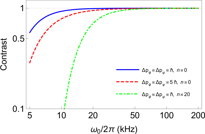
Figure 3: The bound of the spin contrast as a function of the initial angular velocity $\omega_{0}$ for different quantum uncertainties of the angular momentum $I\omega_{0}$. In this plot, we take the same parameters as in Fig.2. The dotted-dished curve shows the contrast in the finite temperature case, where $n=k_{B}T/(\hbar\omega_{0})$. We can see that, in the case of $\omega_{0}=50$kHz, the contrast is still close to 1 when $n=20$ ($T\sim 0.2$mK, which is achievable based on recent rotational cooling technologies [62]).

As we can see, the final SGI contrast is protected by large values of $\omega_{0}$, which reduces all mismatch $\delta\phi=-\delta\psi\propto\omega_{0}^{-1}$, and $\delta\theta\propto\omega_{0}^{-2}$. Besides, to ensure the NV spin’s coherence, the rotation momentum’s uncertainty should be minimized. As shown in Fig.3, the value of $\sigma$ is better to be $\Delta p_{\psi}\sim\hbar$ or even smaller. According to the recently reported experiment about rotating levitated ND [39], the linewidth of rotational frequency $\omega_{0}$ is measured on the order of $10^{-4}$Hz for ND with raduis $264$nm ($m\approx 3\times 10^{-16}$kg ) when $\omega_{0}=100$kHz, which the cooresponding uncertainty $\sigma=I\Delta\omega\approx 7\hbar$. So, current ND rotation control techniques can be applied to protect spin contrast in future SGI experiments.

We can extend our estimation at finite temperature $T$, the initial state of nutation mode can be considered as $\rho_{th}=\int d^{2}\alpha P(\alpha)|\alpha\rangle\langle\alpha|$, where $|\alpha\rangle$ represents coherent states and $P(\alpha)$ is the distribution function of the thermal state. The thermal noise causes a dropping of the overlap between the two nutation states of the two SGI arms, which can be qualified as the $(1+2n)$ factor multiplying the last term in the exponential of (16)(see appendix.D), where $n=k_{B}T/(\hbar\omega_{0})$. An example with $n=20$ is shown in Fig.3.

Discussion: We proposed that, without changing the SGI scheme, giving an appropriate initial angular momentum along the superposition direction to the massive object can cure the interferometry contrast loss induced by the rotational dynamics of the object. Because gyroscope stability is a universal property of fast-spinning objects, the method is scheme-independent and can be applied to other SGI models. Remarkably, the quantum wave packet of the two SGI arms is symmetric in our model, which avoids the contrast loss induced by asymmetric quantum uncertainty evolution (see [33] and appendix.A). In other words, only contrast loss is caused by the classical mismatch of the two angular trajectories. Moreover, the process does not require fine-tuning of experimental parameters. There is no constraint on the location of the NV centre in the ND. The only assumption is that the shape of ND is spherically symmetric. If the ND is not a sphere, we require that the NV axis orient to the principle axis with maximum or minimum inertia moment because objects are rotationally unstable around the axis of intermediate inertia moment, see[63, 35]. A detailed analysis is pending for a future paper.

Acknowledgements: T.Z is supported by the China Scholarship Council (CSC). S.B and A.M are supported by Sloan and the Gordon and Betty Moore foundations. The authors would also like to thank Yoni Japha and Ron Folman for the insightful discussions regarding their findings.

Appendix A Initially static object with no rotation

We will discuss the case when ND is initially static, for the sake of completeness, namely $\omega_{0}=0$. The Zeeman term $\mu sB{\rm cos}\theta$ in the ND’s Hamiltonian implies that the ND with $s=-1$ state is rotationally stable when $\theta=0$, conversely, ND with $s=+1$ is unstable [33, 53]. To avoid a large rotation of angle $\theta$, we use the NV spin state superposition of $s=0$ and $s=-1$ state to create a spatial superposition of ND. From the Hamiltonian Eq.(1) of the ND, the equations of spatial and rotational motion are

$$m\ddot{z}=-\frac{-\chi_{\rho}m}{\mu_{0}}B_{c}\tilde{\eta}-\mu s\tilde{\eta}{\rm cos}\theta\,,$$ (17)

$$\ddot{\theta} =\mu s[B_{nv}\,{\rm sin}\theta+\,\tilde{\eta}d\,{\rm sin}(\theta+\alpha){\rm cos}\theta]$$

$$\approx s\,\omega^{2}(t)\left(\theta-\frac{\tilde{\eta}d\,{\rm sin}\alpha}{B_{c}}\right)\,,$$ (18)

where $B_{nv}=B_{c}+\tilde{\eta}d{\rm cos}(\theta+\alpha)$ and the libration frequency $\omega(t)=\sqrt{\mu B_{c}(t)/I}$. Assuming that the spatial and angular initial state is prepared as ground states in the traps of $z$ and $\theta$ d.o.f., namely $z(0)=\dot{z}(0)=\theta(0)=\dot{\theta}(0)=0$, the numerical solutions of the equation of motions for the two SGI paths are illustrated in Fig.4, 6.

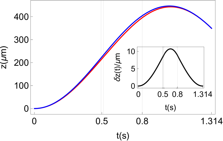
Figure 4: The red curve and blue curve represent the spatial trajectories $z(t)$ of the ND with initial NV spin state $s=-1$ and $s=0$, respectively. We reverse the NV spin state between $\lvert 0\rangle$ and $\lvert-1\rangle$ at $\tau_{3}=0.800s$. The position and translational momentum of the two arms can match at $\tau_{4}=1.314s$. In this plot, we set $m=10^{-17}kg$, $B_{0}=100G$, $B_{1}=1.0G$, $\eta=0.45G/\mu m$, $\tau_{1}=0.494s$, $\tau_{2}=0.513s$, $d=10nm$, $\alpha=\pi/6$. The maximum of the superposition size $\delta z(t)$ is about 10$\mu m$.

Figure 5: The red curve and blue curve represent the spatial trajectories $z(t)$ of the ND with initial NV spin state $s=\pm 1$, respectively. We reverse the NV spin state between $\lvert+1\rangle$ and $\lvert-1\rangle$ at $\tau_{3}=0.8022s$. In this plot, we set $m=10^{-17}$kg, $B_{0}=100G$, $B_{1}=1.0G$, $\eta=0.45G/\mu m$, $\tau_{1}=0.482s$, $\tau_{2}=0.514s$, $d=10{\rm nm}$, $\alpha=\pi/6$. We reverse the NV spin state between $\lvert+1\rangle$ and $\lvert-1\rangle$ at $\tau_{3}=0.8022s$. The spatial trajectory of the two SGI arms closed at $\tau_{4}=1.320s$. The scheme has double superposition size $\delta z$ compared with the scheme using the spin superposition state of $s=-1$ and $s=0$.

The two spatial trajectories can overlap when we choose appropriate values of $\tau_{1}$, $\tau_{2}$, $\tau_{3}$ and $\tau_{4}$. However, the superposition size will be halved compared to the same SGI scheme with $s=\pm 1$. Even worse, the angular trajectories of the two paths can not recombine well finally because the trajectory with initial NV state $s=-1$(see the red curve in Fig.(6) deviates from $\theta=0$ a lot at $t=\tau_{4}$ in the context of the magnetic field profile chosen in Eq. (2). To estimate the final mismatch of the trajectories of $\theta$, we describe the oscillation of $\theta$ as $A{\rm cos}(\omega(t-\tau_{3})+\gamma_{\theta})$ when $t\rightarrow\tau_{3}$, where the amplitude can be estimated by $A\approx\eta d{\rm sin}\alpha/B_{1}$, $\omega=\sqrt{\mu B_{c}(\tau_{3})/I}$, and $\gamma_{\theta}$ represents the oscillation phase at $t=\tau_{3}$. Therefore, at $t=\tau_{3}$, we have $\dot{\theta}(\tau_{3})=A\omega{\rm sin}\gamma_{\theta}$. Then, because the NV spin state is flipped to the $s=0$ state, there is no torque acting on the ND, so the ND rotate with constant angular velocity $\dot{\theta}(\tau_{3})$ until the $t=\tau_{4}$. The final mismatch of $\theta$ reads:

$$\delta\theta(\tau_{4}) \approx\dot{\theta}(\tau_{3})\times(\tau_{4}-\tau_{3})$$

$$\approx\frac{\eta d{\rm sin}\alpha}{B_{1}}\sqrt{\frac{\mu B_{0}}{I}}(\tau_{4}-\tau_{3}){\rm sin}\gamma_{\theta}\,,$$ (19)

where we have used $B_{c}(\tau_{3})\approx B_{0}$. And the mismatch of angular momentum is estimated by

$$\delta p_{\theta}(\tau_{4})\approx I\frac{\eta d{\rm sin}\alpha}{B_{1}}\sqrt{\frac{\mu B_{0}}{I}}{\rm sin}\gamma_{\theta}\,.$$ (20)

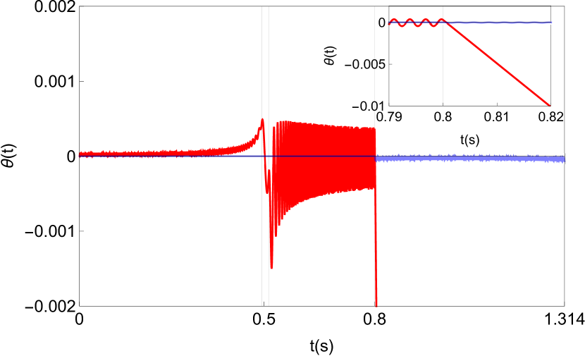
Figure 6: The red curve and blue curve represent the trajectories $\theta(t)$ for the ND with initial NV spin state $s=-1$ and $s=0$, respectively. The parameters we set are the same as in Fig.4. Before $t=\tau_{3}=0.800$s, the ND with $s=-1$ state shows libration with frequency $\omega=\sqrt{\mu B_{c}/I}$. After $t=\tau_{3}$, the spin turns to $s=0$ state so that the ND will freely rotate, which leads to a large final mismatch $\delta\theta(\tau_{4})\sim 0.3$.

We assume the wave packet of $\theta$ is initially a coherent state of the harmonic oscillation mode. At $t=\tau_{3}$, the quantum uncertainties are $\Delta\theta=\sqrt{\hbar/2I\omega}$ and $\Delta p_{\theta}=\sqrt{\hbar I\omega/2}$. At $t=\tau_{4}$, the angular momentum uncertainty remain $\Delta p_{\theta}=\sqrt{\hbar I\omega/2}$ but the angle uncertainty expand to $\Delta\theta(\tau_{4})\approx\hbar(\tau_{4}-\tau_{3})/(2m\Delta\theta(\tau_{3}))$. Therefore, the coherent length of the Gaussian wave packet in angular and angular momentum space can be estimated by[3, 64, 53]

$$\lambda_{\theta}\approx\frac{\hbar}{\Delta p_{\theta}}\,,\ \lambda_{p}\approx\frac{\hbar}{\Delta\theta}\,,$$ (21)

and the spin contrast for two Gaussian wave packets with the same coherent length can be estimated by

$$C\approx exp\left[-\frac{1}{2}\left(\frac{\delta\theta^{2}}{\lambda_{\theta}^{2}}+\frac{\delta p_{\theta}^{2}}{\lambda_{p}^{2}}\right)\right]\,.$$ (22)

For the SGI example shown in Fig.4,6, the coherent length is about $\lambda_{\theta}\sim 0.002$ and $\lambda_{p}\sim I\times 0.003/s$. It means that the classical mismatch $\delta\theta$ and $\delta\dot{\theta}$ should be on or smaller than the order of $10^{-3}$Rad and $10^{-3}{\rm Rad/s}$ respectively to obtain enough contrast. However, as shown in Fig.6, when $d=10$nm and $\alpha=\pi/6$, the final mismatch is about $\delta\theta\approx 0.3$ and $\delta\dot{\theta}\sim 0.6/s$, which are much greater than the coherent length of the wave packet. So, the final contrast is almost zero. To get enough contrast, according to the equation (A,20), one can take the parameters $d$ and $\alpha$ satisfying $|d\,{\rm sin}\alpha|\lesssim 0.05$nm, for the parameters set in Fig.4,6, which is a strong constrain for the crystal structure.

Remarkably, even if $d\,{\rm sin}\alpha=0$, i.e. the mismatch $\delta\theta$ and $\delta p_{\theta}$ of classical trajectories vanish, the contrast loss is still unavoidable because of the asymmetric quantum evolution of wave packet of the two SGI arms, which is named ”quantum uncertainty limit” of spin contrast in [33]. The following form can describe the Gaussian wave function for the two SGI arms

$$\Psi_{a}=\left(\frac{1}{2\pi\sigma_{a}^{2}}\right)^{\frac{1}{4}}exp\left(-\frac{\theta^{2}}{4\sigma_{a}^{2}}+\frac{i\beta_{a}\theta^{2}}{2}\right)\,,$$ (23)

where $\sigma_{a}(t)$ is the quantum uncertainty of the Gaussian wave packet and $a\rightarrow\{L,R\}$ labels the left and right arm of the SGI. According to the Schrodinger equation, the variable $\beta(t)=I\dot{\sigma}_{a}/(\hbar\sigma_{a})$ relate to the expansion rate of the Gaussian wave packet[34]. Therefore, the contrast is

$$C\equiv\int_{-\infty}^{\infty}d\theta\,\Psi_{L}\Psi_{R}^{*}$$

$$=\left[\left(1+\frac{(\sigma_{L}-\sigma_{R})^{2}}{2\sigma_{L}\sigma_{R}}\right)^{2}+(\beta_{L}-\beta_{R})^{2}\sigma_{L}^{2}\sigma_{R}^{2}\right]^{-\frac{1}{4}}$$

$$=\left[\left(1+\frac{(\sigma_{L}-\sigma_{R})^{2}}{2\sigma_{L}\sigma_{R}}\right)^{2}+\frac{I^{2}}{\hbar^{2}}(\dot{\sigma}_{L}\sigma_{R}-\dot{\sigma}_{R}\sigma_{L})^{2}\right]^{-\frac{1}{4}}\,.$$ (24)

Let us label the SGI path with $s=-1$ initial state as the left arm. During $t<\tau_{3}$, the Gaussian wave packet is trapped in harmonic potential so that the uncertainty remains $\sigma_{L}(t)\approx\sigma_{L}(0)=\sqrt{\hbar/(2I\omega(0))}\equiv\sigma_{0}$. When $t>\tau_{3}$, due to $s=0$, the Gaussian wave packet is not affected by the harmonic trap so that the uncertainty of $\theta$ will expand, satisfying

$$\sigma_{L}(t)\approx\frac{\hbar}{2I\sigma_{0}}(t-\tau_{3})\,,\quad t>\tau_{3}\,.$$ (25)

For the right arm, during $t<\tau_{3}$, the spin state is $s=0$, so the wave packet is free to expend. When $t=\tau_{3}$, the uncertainty has expended to $\sigma_{R}(\tau_{3})\approx\hbar\tau_{3}/(2I\sigma_{0})$. After $t=\tau_{3}$, the spin state turns to $s=-1$, then the wave function’s evolution will change from expansion to oscillation. Under the adiabatic approximation $\dot{\omega}\ll\omega^{2}$, the solution of uncertainty oscillation can take the form as(see more calculations in [34])

$$\sigma_{R}(t) \approx\sigma_{R}(\tau_{3})\sqrt{{\rm cos}^{2}\gamma_{\sigma}+\frac{\hbar^{2}}{4I^{2}\omega^{2}\sigma_{R}^{4}(\tau_{3})}{\rm sin}^{2}\gamma_{\sigma}}$$

$$\approx\frac{\hbar\tau_{3}}{2I\sigma_{0}}|{\rm cos}\gamma_{\sigma}|\,,\quad t>\tau_{3}\,,$$ (26)

where $\gamma_{\sigma}\equiv\int_{\tau_{3}}^{t}\omega(t^{\prime})dt^{\prime}$ represents the phase of the uncertainty oscillation and we have used $\sigma_{R}(\tau_{3})\gg\sqrt{\hbar/(2I\omega(t))}\approx\sigma_{0}$ at the second step because $\omega\tau_{3}\gg 1$.

Figure 7: Left panel: The evolution nearing $t=\tau_{4}$ of the contrast induced by the two asymmetric Gaussian wave packets of the SGI model. In this plot, we set $d=0$ so there is no classical mismatch between the two Gaussian wave packets. Other parameters are set the same as in Fig.4. We can see that there are periodically occurring peaks of contrast, and the frequency is about $2\omega(\tau_{4})\sim 2\pi\times 300$Hz. Right panel: Enlarged plot for a contrast peak. The contrast peaks are very sharp, so the time scale of fine-tuning to obtain enough contrast should be much smaller than the order of microseconds.

Therefore, applying (25,A) to (A), we get the evolution for the overlap of the two asymmetric wave packets, as illustrated in Fig.7. The contrast oscillates with frequency $2\omega$(also shown in other models, e.g. [33, 53]). By fine-tuning the final spin measurement time $\tau_{4}$, it is possible to reach a contrast peak when $t=\tau_{4}$. However, as shown in the right panel of Fig.7, the precision of fine-tuning should even be at the order of nanoseconds, which is much smaller than the SGI time scale. Moreover, some noise, such as the fluctuation of the magnetic field, can affect the oscillation of the wave packet’s uncertainty, which causes unpredictable shifts of the location of contrast peaks, making fine-tuning more difficult. By the way, considering the thermal noise of the initial state, the contrast will further be reduced by one or more orders of magnitude [33, 53].

Appendix B Einstein de-Hass effect

In the Heisenberg picture, the operator equations of motion for the NV spin and ND’s rotation dynamics are given by[33]

$$\dot{\textbf{s}}=\frac{\mu}{\hbar}(\textbf{B}\times\textbf{s})+\frac{i}{\hbar}[D(\textbf{s}\cdot\hat{\textbf{n}}_{s})^{2},\textbf{s}]\,,$$ (27)

$$\dot{\textbf{L}} =\frac{i}{\hbar}D[(\textbf{s}\cdot\hat{\textbf{n}}_{s})^{2},\textbf{L}]$$

$$=D((\textbf{s}\cdot\hat{\textbf{n}}_{s})(\textbf{s}\times\hat{\textbf{n}}_{s})+(\textbf{s}\times\hat{\textbf{n}}_{s})(\textbf{s}\cdot\hat{\textbf{n}}_{s}))$$

$$=-i[D(\textbf{s}\cdot\hat{\textbf{n}}_{s})^{2},\textbf{s}]\,,$$ (28)

$$\dot{\hat{\textbf{n}}}_{i}=\frac{i}{\hbar}\sum_{k}\left[\frac{L_{k}^{2}}{I_{k}},\,\hat{\textbf{n}}_{i}\right]=\boldsymbol{\omega}\times\hat{\textbf{n}}_{i}+i\gamma\hat{\textbf{n}}_{i}\,,$$ (29)

where $i=\{1,2,3\}$ labels the index in the rotating frame and $\gamma=\hbar\sum_{k}(1/2I_{k})$.

$$\dot{s}_{i} =\dot{\textbf{s}}\cdot\hat{\textbf{n}}_{i}+\textbf{s}\cdot\dot{\hat{\textbf{n}}}_{i}$$ (30)

$$=\frac{i}{\hbar}[D(\textbf{s}\cdot\hat{\textbf{n}}_{s})^{2},s_{i}]+\frac{\mu}{\hbar}\varepsilon_{ijk}B_{j}s_{k}+\varepsilon_{ijk}s_{j}\omega_{k}+i\gamma s_{i}\,.$$

For massive objects with $m\gtrsim 10^{-17}$kg, the coefficient $\gamma\sim\hbar/I\lesssim 10^{-8}$Hz is negligible compared with $D\sim$GHz, $\mu B/\hbar\sim$ MHz and $\omega\sim$ kHz. We can define an effective Hamiltonian to describe the spin evolution in the rotating frame

$$H_{s}=DS_{\parallel}^{2}+\mu\textbf{s}\cdot\textbf{B}-\frac{\hbar}{I}\textbf{s}\cdot\textbf{L}\,.$$ (31)

It can be verified that the Hamiltonian equation $\dot{s}_{i}=i[H_{s},s_{i}]/\hbar$ is consistent with (30). For our SGI model, applying the basis $\{s_{1},s_{2},s_{3}\}$, the effective spin Hamiltonian is

$$H_{s}=\begin{pmatrix}\Delta_{+}&We^{-i\omega_{0}t}&0\\ We^{i\omega_{0}t}&0&We^{-i\omega_{0}t}\\ 0&We^{i\omega_{0}t}&\Delta_{-}\end{pmatrix}\,,$$ (32)

where

$$\Delta_{\pm}\equiv D\pm\mu B{\rm cos}\theta_{0}\mp\hbar\omega_{0},\ W\equiv\frac{\mu B{\rm sin}\theta_{0}}{\sqrt{2}}\,.$$ (33)

In the resonant case $\hbar\omega_{0}\approx D\pm\mu B{\rm cos}\theta_{0}$, $s_{3}=+1$(or $s_{3}=-1$) state would degenerate with the $s_{3}=0$ state, which means that any small off-diagonal term $W$ would leads to Rabi oscillation between $s_{3}=\pm 1$ and $s=0$ state. To mitigate the amplitude of the Rabi oscillation, we take the off-resonant condition $\hbar\omega_{0}\ll D\pm\mu B{\rm cos}\theta_{0}$. Then, we have $|\Delta_{\pm}|\gg W$, so the Rabi oscillation is negligible. Therefore, the spin components in the rotating frame is stable during the interferometry process, i.e. $\dot{s}_{i}=0$.

According to the equation (27,B,29) and $\dot{s}_{i}=0$, we can get the evolution of ND’s rotational angular momentum

$$\dot{L}_{i} =\textbf{L}\cdot\dot{\hat{\textbf{n}}}_{i}+\dot{\textbf{L}}\hat{\textbf{n}}_{i}=\textbf{L}\cdot\dot{\hat{\textbf{n}}}_{i}+\mu(\textbf{B}\times\textbf{s})\cdot\hat{\textbf{n}}_{i}-\hbar\dot{\textbf{s}}\cdot\hat{\textbf{n}}_{i}$$

$$=\varepsilon_{ijk}\left(\mu B_{j}s_{k}+\hbar s_{j}\frac{L_{k}}{I_{k}}+L_{j}\frac{L_{k}}{I_{k}}\right)\,,$$ (34)

where the first term represents the Zeeman torque, the second term is the torque due to the Einstein-de Hass effect, and the last term vanish if the shape of the ND is spherical.

Appendix C Classical evolution of the nutation mode

The evolution of $\theta(t)$ is governed by the equation

$$\ddot{\theta}=-\left(\omega_{0}^{2}-\frac{\mu sB_{c}}{I}\right)(\theta-\theta_{0})+\frac{\mu sB_{c}\theta_{0}}{I}\,.$$ (35)

The equation can be rewritten as

$$\ddot{\theta}=-\omega^{2}(t)(\theta-\bar{\theta}(t))\,,$$ (36)

where

$$\omega^{2}(t)\equiv\omega_{0}^{2}-\frac{\mu sB_{c}(t)}{I}\approx\omega_{0}^{2}\,,$$ (37)

$$\bar{\theta}(t)\equiv\theta_{0}+\frac{\mu sB_{c}(t)\theta_{0}}{I\omega_{0}^{2}-\mu sB_{c}(t)}\approx\theta_{0}+\frac{\mu sB_{c}(t)\theta_{0}}{I\omega_{0}^{2}}\,.$$ (38)

For SGI models with long timescale $\sim 1s$, the variation of $B_{c}(t)$ is much slower than the oscillation of $\theta(t)$ with frequency $\omega_{0}\sim$kHz-MHz. So, equation (36) can be regarded as an equation of harmonic oscillator with adiabatically changing parameters. Therefore, we can take the ansatz for the solution the oscillation

$$\theta(t)=A_{\theta}{\rm cos}(\omega t)+\bar{\theta}\,.$$ (39)

Assuming the initial condition $\theta(0)=\theta_{0}$ and $\dot{\theta}(0)=0$, we get the initial amplitude of the nutation mode

$$A_{\theta}(t)=\frac{\mu B_{0}\theta_{0}}{I\omega_{0}^{2}},\quad 0\leq t<\tau_{3}\,.$$ (40)

At $t=\tau_{3}$, we flip the NV spin between $s=+1$ and $s=-1$ and then the equilibrium position $\bar{\theta}$ is changed

$$\delta\bar{\theta}(\tau_{3})=\frac{2\mu B_{c}(\tau_{3})\theta_{0}}{I\omega_{0}^{2}}\,.$$ (41)

The rapid change of $\bar{\theta}$ kicks the oscillator, then the amplitude after the spin flipping satisfies

$$|A_{\theta}(0)-\delta\bar{\theta}(\tau_{3})|\leq A_{\theta}(t)\leq|A_{\theta}(0)+\delta\bar{\theta}(\tau_{3})|,\ t>\tau_{3}\,.$$ (42)

In our SGI model, we have $B_{c}(\tau_{4})\sim B_{c}(\tau_{3})\lesssim B_{0}$. Therefore, the bound of oscillation amplitude can be estimated by $A_{\theta}(0)\lesssim A_{\theta}(t>\tau_{3})\lesssim 3A_{\theta}(0)$.

At $t=\tau_{4}$, there is a mismatch of $\bar{\theta}(t)$ between the two SGI paths, namely $\delta\bar{\theta}(\tau_{4})=2\mu B_{c}(\tau_{4})\theta_{0}/I\omega_{0}^{2}$. The final mismatch $\delta\theta$ of $\theta(\tau_{4})$ between the two paths can be roughly estimated by $\delta\bar{\theta}(\tau_{4})$ and $A_{\theta}(\tau_{4})$, namely

$$\delta\theta<A_{\theta L}(\tau_{4})+A_{\theta R}(\tau_{4})+\delta\bar{\theta}(\tau_{4})\lesssim\frac{8\mu}{I\omega_{0}^{2}}B_{0}\theta_{0}\,,$$ (43)

where we have taken the upper bound of the oscillation amplitude $A_{\theta}(\tau_{4})\lesssim 3\mu B_{0}\theta_{0}/I\omega_{0}^{2}$ for both the left and right paths.

Appendix D Quantum evolution of angular wave packets

According to the canonical quantization procedure, we have $[\hat{\theta},\hat{p}_{\theta}]=[\hat{\phi},\hat{p}_{\phi}]=[\hat{\psi},\hat{p}_{\psi}]=i\hbar$, and $[\hat{p}_{\phi},\hat{p}_{\psi}]=[\hat{p}_{\theta},\hat{p}_{\phi}]=[\hat{p}_{\psi},\hat{p}_{\theta}]=0$, which are consistent with the commutation relations of angular momentum [65], i.e. $[\hat{L}_{i},\hat{L}_{j}]=i\varepsilon_{ijk}\hat{L}_{k}$, where $\{i,j,k\}$ label $\{x,y,z\}$ or $\{1,2,3\}$. First, we define the shifted operators

$$\hat{\theta}^{\prime}\equiv\hat{\theta}-\theta_{0}-\frac{\mu sB_{c}\theta_{0}}{I\omega_{0}^{2}}\,,\ \hat{p}^{\prime}_{\phi}\equiv\hat{p}_{\phi}-\langle\hat{p}_{\phi}\rangle\,,\ \hat{p}^{\prime}_{\psi}\equiv\hat{p}_{\psi}-\langle\hat{p}_{\psi}\rangle\,,$$ (44)

where $\langle\hat{p}_{\phi}\rangle=I\omega_{0}{\rm cos}\theta_{0}$, $\langle\hat{p}_{\psi}\rangle=I\omega_{0}$ are the expectation values of $\hat{p}_{\phi}$ and $\hat{p}_{\psi}$. The quantum Hamiltonian of rotational dynamics (7) can be written as

$$\hat{H}\approx\frac{\hat{p}_{\theta}^{2}}{2I}+\frac{1}{2}I\omega^{2}_{0}\hat{\theta}^{\prime 2}+g(\hat{p}^{\prime}_{\phi},\hat{p}^{\prime}_{\psi},t)-f(\hat{p}^{\prime}_{\phi},\hat{p}^{\prime}_{\psi})\hat{\theta}^{\prime}\,,$$ (45)

where the function $f$ and $g$ is defined as

$$g(p^{\prime}_{\phi},p^{\prime}_{\psi},t)=\frac{(p^{\prime}_{\phi}-p^{\prime}_{\psi})^{2}}{2I\theta_{0}^{2}}-\omega_{0}p^{\prime}_{\psi}-\frac{\mu sB_{c}}{I\omega_{0}}(p^{\prime}_{\phi}-p^{\prime}_{\psi})\,,$$

$$f(p^{\prime}_{\phi},p^{\prime}_{\psi})=\frac{\omega_{0}}{\theta_{0}}(p^{\prime}_{\phi}-p^{\prime}_{\psi})+\frac{(p^{\prime}_{\phi}-p^{\prime}_{\psi})^{2}}{I\theta_{0}^{3}}\,.$$ (46)

We neglect higher order terms of $\hat{\theta}^{\prime}$ based on assumption $\langle\hat{\theta}^{\prime}\rangle\ll\theta_{0}\ll 1$ and we assume that the quantum fluctuation of momentum is small, namely $\Delta p_{\phi}\approx\Delta p_{\psi}\sim\hbar\ll I\omega_{0}$.

Initially, the spin state is $s=0$, and the quantum wave packet of $\phi$ and $\psi$ degree of freedom in momentum space is set as Gaussian wave packets with width $\Delta p_{\phi}$ and $\Delta p_{\psi}$, respectively. The quantum state of the nutation mode $\theta$ is set as the ground state $\lvert 0\rangle_{\bar{\theta}_{0}}$ in the harmonic trap with frequency $\omega_{0}$ and equilibrium position $\bar{\theta}_{0}$. So the initial wave function of angular d.o.f. is

$$\lvert\Psi(0)\rangle=\int\frac{dp^{\prime}_{\phi}\,dp^{\prime}_{\psi}}{\sqrt{2\pi\Delta p_{\phi}\Delta p_{\psi}}}\,e^{-\frac{(p^{\prime}_{\phi})^{2}}{4\Delta p_{\phi}^{2}}}e^{-\frac{(p^{\prime}_{\psi})^{2}}{4\Delta p_{\psi}^{2}}}\lvert p^{\prime}_{\phi},p^{\prime}_{\psi}\rangle\otimes|0\rangle_{\bar{\theta}_{0}}\,.$$ (47)

From the Hamiltonian (45), the initial equilibrium position $\bar{\theta}$ of the $\theta$ mode is

$$\bar{\theta}_{0}(p^{\prime}_{\phi},p^{\prime}_{\psi})=\theta_{0}+\frac{f(p^{\prime}_{\phi},p^{\prime}_{\psi})}{I\omega_{0}^{2}}\,.$$ (48)

We can see that the equilibrium position of the harmonic trap is also shifted by the quantum fluctuations $p^{\prime}_{\phi}$ and $p^{\prime}_{\psi}$. When the interferometer starts, the spin state is prepared as a superposition state of $s=+1$ and $s=-1$. Then $\bar{\theta}$ deviates from the initial equilibrium position $\bar{\theta}_{0}$ so that the ground state $|0\rangle_{\bar{\theta}_{0}}$ becomes a coherent state in the harmonic trap with new balance position

$$\bar{\theta}(s,t,p^{\prime}_{\phi},p^{\prime}_{\psi})=\theta_{0}+\frac{\mu sB_{c}(t)\theta_{0}+f(p^{\prime}_{\phi},p^{\prime}_{\psi})}{I\omega_{0}^{2}}\,.$$ (49)

Therefore, the quantum evolution of wave packet is given by

$$\lvert\Psi(t)\rangle=exp\left(-\frac{i}{\hbar}\int\hat{H}dt\right)\lvert\Psi(0)\rangle$$

$$=\int\frac{dp^{\prime}_{\phi}\,dp^{\prime}_{\psi}}{\sqrt{2\pi\Delta p_{\phi}\Delta p_{\psi}}}\,e^{-\frac{(p^{\prime}_{\phi})^{2}}{4\Delta p_{\phi}^{2}}}e^{-\frac{(p^{\prime}_{\psi})^{2}}{4\Delta p_{\psi}^{2}}}$$

$$\times exp\left[-\frac{i}{\hbar}\int dt\,g(p^{\prime}_{\phi},p^{\prime}_{\psi},t)+f(p^{\prime}_{\phi},p^{\prime}_{\psi})\hat{\theta}^{\prime}\right.$$

$$+\left.\frac{\hat{p}_{\theta}^{2}}{2I}+\frac{1}{2}I\omega^{2}_{0}\hat{\theta}^{\prime 2}\right]\lvert p^{\prime}_{\phi},p^{\prime}_{\psi}\rangle\otimes|\alpha\rangle$$

$$=\int\frac{dp^{\prime}_{\phi}\,dp^{\prime}_{\psi}}{\sqrt{2\pi\Delta p_{\phi}\Delta p_{\psi}}}\,e^{-\frac{(p^{\prime}_{\phi})^{2}}{4\Delta p_{\phi}^{2}}}e^{-\frac{(p^{\prime}_{\psi})^{2}}{4\Delta p_{\psi}^{2}}}$$

$$\times exp\left[-\frac{i}{\hbar}\int dt\,g(p^{\prime}_{\phi},p^{\prime}_{\psi},t)\right]\lvert p^{\prime}_{\phi},p^{\prime}_{\psi}\rangle\otimes|\alpha(t)\rangle_{\bar{\theta}}\,,$$ (50)

and, near $t=0$, the coherent state $\lvert\alpha(t)\rangle_{\bar{\theta}}$ is evolving as

$$\lvert\alpha(t)\rangle_{\bar{\theta}} =exp\left[\frac{-i}{\hbar}\int dt\,\frac{\hat{p}_{\theta}^{2}}{2I}+\frac{I\omega^{2}_{0}}{2}\hat{\theta}^{\prime 2}-f(p^{\prime}_{\phi},p^{\prime}_{\psi})\hat{\theta}^{\prime}\right]|0\rangle_{\bar{\theta}_{0}}$$

$$=\bigg{|}-\sqrt{\frac{I\omega_{0}}{2\hbar}}\frac{\mu sB_{0}\theta_{0}}{I\omega_{0}^{2}}e^{-i\omega_{0}t}\Bigg{\rangle}_{\bar{\theta}}\,.$$ (51)

Since both of $\bar{\theta}$ and $\bar{\theta}_{0}$ are shifted by $f/(I\omega^{2}_{0})$, the quantum fluctuation of momentum $p_{\phi}$ and $p_{\psi}$ do not affect the initial amplitude of the nutation mode. The evolution of the amplitude $|\alpha|$ of the coherent state can be obtained from the analysis of classical amplitude estimation in appendix.C, where the final amplitude $|\alpha|$ satisfies

$$|\alpha(\tau_{4})|<\sqrt{\frac{I\omega_{0}}{2\hbar}}\frac{3\mu B_{0}\theta_{0}}{I\omega_{0}^{2}}\,.$$ (52)

For the quantum state of $\psi$ and $\phi$, since the Hamiltonian only consists of quadratic terms of $\hat{p}^{\prime}_{\phi}$ and $\hat{p}^{\prime}_{\psi}$, the wave packet of $\phi$ and $\psi$ remain the Gaussian form during the evolution. And because of $[\hat{p}^{\prime}_{\phi},\hat{H}]=0$ and $[\hat{p}^{\prime}_{\psi},\hat{H}]=0$, the momentum uncertainty $\Delta p_{\phi}$ and $\Delta p_{\psi}$ are invariant.

From the solution (D) of the angular quantum state, we can figure out the SGI contrast for the rotational dynamics, which is given by

$$C =|\langle\Psi_{L}(\tau_{4})|\Psi_{R}(\tau_{4})\rangle|=\int\frac{dp^{\prime}_{\phi}\,dp^{\prime}_{\psi}dp^{\prime\prime}_{\phi}\,dp^{\prime\prime}_{\psi}}{2\pi\Delta p_{\phi}\Delta p_{\psi}}$$

$$\times e^{-\frac{(p^{\prime}_{\phi})^{2}+(p^{\prime\prime}_{\phi})^{2}}{4\Delta p_{\phi}^{2}}}e^{-\frac{(p^{\prime}_{\psi}+(p^{\prime\prime}_{\psi})^{2})^{2}}{4\Delta p_{\psi}^{2}}}$$

$$\times exp\left[-\frac{i}{\hbar}\int_{0}^{\tau_{4}}dt(g_{L}(p^{\prime}_{\phi},p^{\prime}_{\psi},t)-g_{R}(p^{\prime\prime}_{\phi},p^{\prime\prime}_{\psi},t))\right]$$

$$\times\langle p^{\prime}_{\phi},p^{\prime}_{\psi}\lvert p^{\prime\prime}_{\phi},p^{\prime\prime}_{\psi}\rangle\times\langle\alpha_{L}(p^{\prime}_{\phi},p^{\prime}_{\psi},\tau_{4})\lvert\alpha_{R}(p^{\prime\prime}_{\phi},p^{\prime\prime}_{\psi},\tau_{4})\rangle$$

$$=\int\frac{dp^{\prime}_{\phi}\,dp^{\prime}_{\psi}}{2\pi\Delta p_{\phi}\Delta p_{\psi}}\,e^{-\frac{(p^{\prime}_{\phi})^{2}}{2\Delta p_{\phi}^{2}}}e^{-\frac{(p^{\prime}_{\psi})^{2}}{2\Delta p_{\psi}^{2}}}$$

$$\times exp\left[-\frac{i}{\hbar}\int_{0}^{\tau_{4}}dt(g_{L}(p^{\prime}_{\phi},p^{\prime}_{\psi},t)-g_{R}(p^{\prime}_{\phi},p^{\prime}_{\psi},t))\right]$$

$$\times|\leftindex_{\bar{\theta}_{L}}{\langle}\alpha_{L}(p^{\prime}_{\phi},p^{\prime}_{\psi},\tau_{4})\lvert\alpha_{R}(p^{\prime}_{\phi},p^{\prime}_{\psi},\tau_{4})\rangle_{\bar{\theta}_{R}}|\,,$$ (53)

in which we have

$$\int_{0}^{\tau_{4}}dt\,[g_{L}(p^{\prime}_{\phi},p^{\prime}_{\psi},t)-g_{R}(p^{\prime}_{\phi},p^{\prime}_{\psi},t)]$$

$$=\int_{0}^{\tau_{4}}dt\left(\frac{\mu sB_{c}}{I\omega_{0}}\bigg{|}_{L}-\frac{\mu sB_{c}}{I\omega_{0}}\bigg{|}_{R}\right)(p^{\prime}_{\phi}-p^{\prime}_{\psi})$$

$$=\delta\phi\times(p^{\prime}_{\phi}-p^{\prime}_{\psi})\,.$$ (54)

$\delta\phi$, evaluated in (15), is the mismatch between the classical trajectory of $\phi$ of the left and right SGI arms. The module of the inner product $\leftindex_{\bar{\theta}_{L}}{\langle}\alpha_{L}(p^{\prime}_{\phi},p^{\prime}_{\psi},\tau_{4})\lvert\alpha_{R}(p^{\prime}_{\phi},p^{\prime}_{\psi},\tau_{4})\rangle_{\bar{\theta}_{R}}$ of two coherent states is determined by the distance of the complex variables $\alpha_{L}$ and $\alpha_{R}$, namely

$$|\leftindex_{\bar{\theta}_{L}}{\langle}\alpha_{L}\lvert\alpha_{R}\rangle_{\bar{\theta}_{R}}|=exp\left[-\frac{1}{2}|\alpha_{L}-(\alpha_{R}+\delta X)|^{2}\right]\,,$$ (55)

where

$$\delta X\equiv\sqrt{\frac{I\omega_{0}}{2\hbar}}|\bar{\theta}_{L}-\bar{\theta}_{R}|=\sqrt{\frac{I\omega_{0}}{2\hbar}}\frac{2\mu B_{c}(\tau_{4})\theta_{0}}{I\omega_{0}^{2}}\,.$$ (56)

Notably, the equilibrium position deviations due to the quantum fluctuation $p^{\prime}_{\phi}$ and $p^{\prime}_{\psi}$ are the same for left and right SGI paths, thus the overlap of the two coherent state $|\leftindex_{\bar{\theta}_{L}}{\langle}\alpha_{L}\lvert\alpha_{R}\rangle_{\bar{\theta}_{R}}|$ is independent on the variable $p^{\prime}_{\phi}$ and $p^{\prime}_{\psi}$.

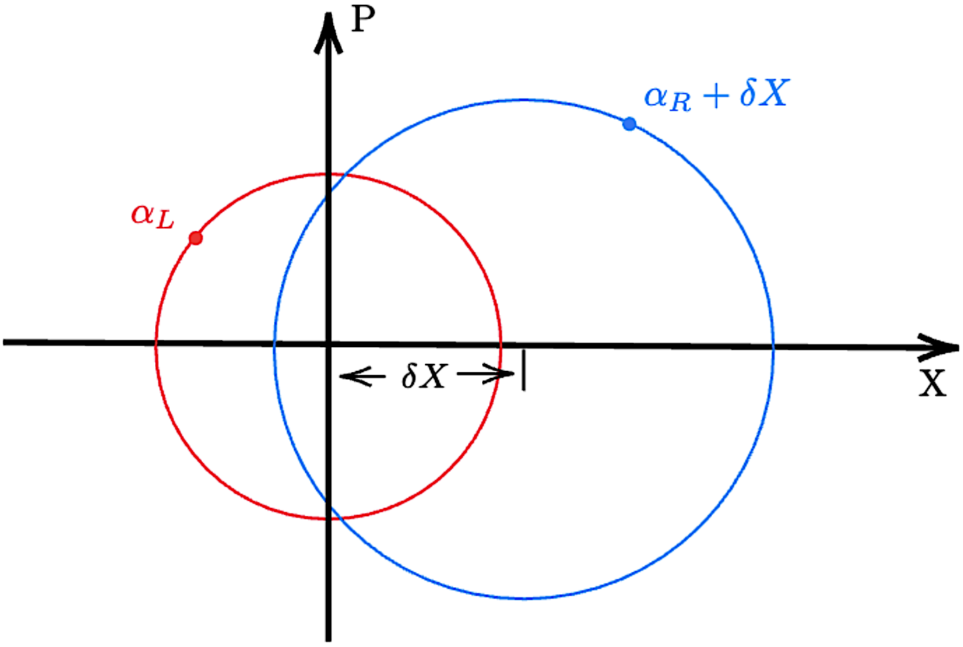
Figure 8: Sketch of coherent state $|\alpha_{L}\rangle$ and $|\alpha_{R}\rangle$ in the phase space $\{X=\sqrt{I\omega_{0}/(2\hbar)}\theta,P=\sqrt{1/(I\omega_{0}2\hbar)}p_{\theta}\}$ at $t\approx\tau_{4}$. The red and blue circle represents the evolution of the two coherent states. The mismatch of dimensionless equilibrium position $\delta X=\sqrt{I\omega_{0}/(2\hbar)}\,\delta\bar{\theta}(\tau_{4})$.

Plugging (D) and (55) into the contrast formula (D), we end up with the contrast

$$C=|\langle\alpha_{L}\lvert\alpha_{R}\rangle|\int\frac{dp^{\prime}_{\phi}\,dp^{\prime}_{\psi}}{2\pi\Delta p_{\phi}\Delta p_{\psi}}\,e^{-\frac{(p^{\prime}_{\phi})^{2}}{2\Delta p_{\phi}^{2}}-\frac{(p^{\prime}_{\psi})^{2}}{2\Delta p_{\psi}^{2}}+\frac{i}{\hbar}\delta\phi(p^{\prime}_{\phi}-p^{\prime}_{\psi})}$$

$$=exp\left[-\frac{1}{2}\left(\delta\phi^{2}\frac{\Delta p_{\phi}^{2}}{\hbar^{2}}+\delta\psi^{2}\frac{\Delta p_{\psi}^{2}}{\hbar^{2}}\right)\right]|\langle\alpha_{L}\lvert\alpha_{R}\rangle|\,.$$ (57)

Using (52),(55) and (56), we obtain the lower bound of the overlap bwteen the two coherent state

$$|\leftindex_{\bar{\theta}_{L}}{\langle}\alpha_{L}\lvert\alpha_{R}\rangle_{\bar{\theta}_{R}}|>exp\left[-\frac{1}{2}\left(|\alpha_{L}|+|\alpha_{R}|+\delta X\right)^{2}\right]$$

$$>exp\left[-\frac{1}{2}\frac{I\omega_{0}}{2\hbar}\left(\frac{8\mu B_{0}\theta_{0}}{I\omega_{0}^{2}}\right)^{2}\right]$$ (58)

Therefore, the lower bound of the contrast is

$$C>e^{-\frac{1}{2}\delta\phi^{2}\frac{\Delta p_{\phi}^{2}}{\hbar^{2}}}e^{-\frac{1}{2}\delta\psi^{2}\frac{\Delta p_{\psi}^{2}}{\hbar^{2}}}exp\left(-\frac{16\mu^{2}B_{0}^{2}\theta_{0}^{2}}{\hbar I\omega_{0}^{3}}\right)\,.$$ (59)

The contrast (59) is calculated in the zero temperature case, that the initial state of nutation mode is the ground state of the harmonic trap. Considering a finite temperature $T$, the initial state of nutation mode can be described by the density matrix operator in the coherent state basis

$$\hat{\rho}_{th}=\int\frac{d^{2}\alpha}{\pi}\frac{e^{-\frac{|\alpha|^{2}}{n}}}{n}|\alpha\rangle\langle\alpha|\,,$$ (60)

in which $n\equiv k_{B}T/(\hbar\omega_{0})$ is the occupation number. We here take the definition of the final overlap between two thermal coherent state as $tr[\hat{D}(\zeta_{L})\hat{\rho}_{th}\hat{D}^{\dagger}(\zeta_{R})]$, where $\hat{D}(\zeta)$ is the displacement operator satisfying $\hat{D}(\zeta_{L})|0\rangle_{\bar{\theta}_{0}}=|\alpha_{L}\rangle_{\bar{\theta}}$ and $\hat{D}(\zeta_{R})|0\rangle_{\bar{\theta}_{0}}=|\alpha_{R}\rangle_{\bar{\theta}}$. Then, we have[66]

$$tr\left[\hat{D}(\zeta_{L})\hat{\rho}_{th}\hat{D}^{\dagger}(\zeta_{R})\right]=exp\left[\varphi-|\Delta\zeta|^{2}\left(\frac{1}{2}+n\right)\right]\,,$$ (61)

where the phase factor $\varphi\equiv(\zeta_{L}\zeta_{R}^{*}-\zeta_{L}^{*}\zeta_{R})/2$ is a imaginary number so it does not contribute on the contrast. Therefore, considering thermal effect, the equation (55) and (D) should be rewrite as

$$|\langle\alpha_{L}\lvert\alpha_{R}\rangle|_{th} =exp\left[-\left(\frac{1}{2}+n\right)|\alpha_{L}-(\alpha_{R}+\delta X)|^{2}\right]$$

$$>exp\left[-\left(\frac{1}{2}+n\right)\frac{32\mu^{2}B_{0}^{2}\theta_{0}^{2}}{\hbar I\omega_{0}^{3}}\right]\,.$$ (62)

The lower bound of the spin contrast in finite temperature case is given by

$$C_{th}>exp\left[-\frac{\delta\phi^{2}\Delta p_{\phi}^{2}}{2\hbar^{2}}-\frac{\delta\psi^{2}\Delta p_{\psi}^{2}}{2\hbar^{2}}-\frac{16(1+2n)\mu^{2}B_{0}^{2}\theta_{0}^{2}}{\hbar I\omega_{0}^{3}}\right]\,.$$ (63)

References

Doherty et al. [2013]M. W. Doherty, N. B. Manson,
P. Delaney, F. Jelezko, J. Wrachtrup, and L. C. Hollenberg, The nitrogen-vacancy colour centre in diamond, Physics Reports 528, 1–45 (2013).
Margalit et al. [2018]Y. Margalit, Z. Zhou,
O. Dobkowski, Y. Japha, D. Rohrlich, S. Moukouri, and R. Folman, Realization of a complete stern-gerlach interferometer (2018), arXiv:1801.02708
[quant-ph] .
Margalit et al. [2021]Y. Margalit, O. Dobkowski,
Z. Zhou, O. Amit, Y. Japha, S. Moukouri, D. Rohrlich, A. Mazumdar, S. Bose, C. Henkel, and R. Folman, Realization of a complete
stern-gerlach interferometer: Toward a test of quantum gravity, Science Advances 7, eabg2879 (2021).
Amit et al. [2019]O. Amit, Y. Margalit,
O. Dobkowski, Z. Zhou, Y. Japha, M. Zimmermann, M. A. Efremov, F. A. Narducci, E. M. Rasel, W. P. Schleich, et al., T 3
stern-gerlach matter-wave interferometer, Physical review letters 123, 083601 (2019).
Marshman et al. [2020a]R. J. Marshman, A. Mazumdar,
G. W. Morley, P. F. Barker, S. Hoekstra, and S. Bose, Mesoscopic Interference for Metric and Curvature (MIMAC)
Gravitational Wave Detection, New J. Phys. 22, 083012 (2020a), arXiv:1807.10830 [gr-qc] .
Wan et al. [2016]C. Wan, M. Scala, S. Bose, A. C. Frangeskou, A. T. M. A. Rahman, G. W. Morley, P. F. Barker, and M. S. Kim, Tolerance in the Ramsey interference of a trapped nanodiamond, Phys. Rev. A 93, 043852 (2016).
Scala et al. [2013]M. Scala, M. S. Kim,
G. W. Morley, P. F. Barker, and S. Bose, Matter-wave interferometry of a levitated thermal
nano-oscillator induced and probed by a spin, Phys. Rev. Lett. 111, 180403 (2013).
Bose et al. [2017]S. Bose, A. Mazumdar,
G. W. Morley, H. Ulbricht, M. Toroš, M. Paternostro, A. Geraci, P. Barker, M. S. Kim, and G. Milburn, Spin Entanglement
Witness for Quantum Gravity, Phys. Rev. Lett. 119, 240401 (2017), arXiv:1707.06050 [quant-ph] .
Marshman et al. [2020b]R. J. Marshman, A. Mazumdar, and S. Bose, Locality and entanglement in table-top testing of
the quantum nature of linearized gravity, Physical Review A 101, 052110 (2020b).
Bose et al. [2023]S. Bose, A. Mazumdar,
M. Schut, and M. Toroš, Entanglement witness for the weak equivalence
principle, Entropy 25, 448 (2023).
Carney et al. [2019]D. Carney, P. C. E. Stamp, and J. M. Taylor, Tabletop experiments for
quantum gravity: a user’s manual, Class. Quant. Grav. 36, 034001 (2019).
Danielson et al. [2022]D. L. Danielson, G. Satishchandran, and R. M. Wald, Gravitationally mediated entanglement: Newtonian field versus gravitons, Phys. Rev. D 105, 086001 (2022).
Christodoulou et al. [2023]M. Christodoulou, A. Di Biagio, M. Aspelmeyer, Č. Brukner, C. Rovelli, and R. Howl, Locally mediated entanglement in linearized
quantum gravity, Physical Review Letters 130, 100202 (2023).
Schut et al. [2022]M. Schut, J. Tilly,
R. J. Marshman, S. Bose, and A. Mazumdar, Improving resilience of quantum-gravity-induced entanglement of
masses to decoherence using three superpositions, Phys. Rev. A 105, 032411 (2022), arXiv:2110.14695 [quant-ph] .
Marshman et al. [2024]R. J. Marshman, S. Bose,
A. Geraci, and A. Mazumdar, Entanglement of magnetically levitated massive
schrödinger cat states by induced dipole interaction, Physical Review A 109, L030401 (2024).
Elahi and Mazumdar [2023]S. G. Elahi and A. Mazumdar, Probing massless and
massive gravitons via entanglement in a warped extra dimension, Physical Review D 108, 035018 (2023).
Chakraborty et al. [2023]S. Chakraborty, A. Mazumdar, and R. Pradhan, Distinguishing jordan and
einstein frames in gravity through entanglement, Physical Review D 108, L121505 (2023).
Toroš et al. [2024a]M. Toroš, M. Schut,
P. Andriolo, S. Bose, and A. Mazumdar, Relativistic Dips in Entangling Power of Gravity, (2024a), arXiv:2405.04661 [quant-ph] .
Toroš et al. [2024b]M. Toroš, P. Andriolo,
M. Schut, S. Bose, and A. Mazumdar, Relativistic Effects on Entangled Single-Electron Traps, (2024b), arXiv:2406.17848 [quant-ph] .
Beckering Vinckers et al. [2023]U. K. Beckering Vinckers, Á. De La Cruz-Dombriz, and A. Mazumdar, Quantum entanglement of masses with nonlocal gravitational interaction, Physical Review D 107, 124036 (2023).
Schut et al. [2023a]M. Schut, A. Grinin,
A. Dana, S. Bose, A. Geraci, and A. Mazumdar, Relaxation of experimental parameters in a quantum-gravity-induced
entanglement of masses protocol using electromagnetic screening, Phys. Rev. Res. 5, 043170 (2023a), arXiv:2307.07536 [quant-ph] .
Fein et al. [2019]Y. Y. Fein et al., Quantum
superposition of molecules beyond 25 kda, Nature Phys. 15, 1242 (2019).
Overstreet et al. [2022]C. Overstreet, P. Asenbaum, J. Curti,
M. Kim, and M. A. Kasevich, Observation of a gravitational aharonov-bohm
effect, Science 375, 226 (2022).
Asenbaum et al. [2017]P. Asenbaum, C. Overstreet, T. Kovachy,
D. D. Brown, J. M. Hogan, and M. A. Kasevich, Phase shift in an atom interferometer due to
spacetime curvature across its wave function, Physical review letters 118, 183602 (2017).
Japha [2021]Y. Japha, Unified model of
matter-wave-packet evolution and application to spatial coherence of atom
interferometers, Physical Review A 104, 053310 (2021).
Ma et al. [2021]Y. Ma, M. Kim, and B. A. Stickler, Torque-free manipulation of
nanoparticle rotations via embedded spins, Physical Review B 104, 134310 (2021).
Jin et al. [2024]Y. Jin, K. Shen, P. Ju, X. Gao, C. Zu, A. J. Grine, and T. Li, Quantum
control and berry phase of electron spins in rotating levitated diamonds in
high vacuum, Nature Communications 15, 5063 (2024).
Chen et al. [2019]X.-Y. Chen, T. Li, and Z.-Q. Yin, Nonadiabatic dynamics and geometric phase of an
ultrafast rotating electron spin, Science Bulletin 64, 380 (2019).
Pedernales et al. [2020]J. S. Pedernales, G. W. Morley, and M. B. Plenio, Motional Dynamical
Decoupling for Interferometry with Macroscopic Particles, Phys. Rev. Lett. 125, 023602 (2020).
Wood et al. [2022a]B. D. Wood, S. Bose, and G. W. Morley, Spin dynamical decoupling for generating
macroscopic superpositions of a free-falling nanodiamond, Phys. Rev. A 105, 012824 (2022a).
Wood et al. [2022b]B. D. Wood et al., Long spin
coherence times of nitrogen vacancy centers in milled nanodiamonds, Phys. Rev. B 105, 205401 (2022b).
Schut et al. [2023b]M. Schut, H. Bosma,
M. Wu, M. Toroš, S. Bose, and A. Mazumdar, Dephasing due to electromagnetic interactions in spatial qubits, (2023b), arXiv:2312.05452 [quant-ph] .
Zhou et al. [2022a]R. Zhou, R. J. Marshman,
S. Bose, and A. Mazumdar, Gravito-diamagnetic forces for mass independent large
spatial quantum superpositions, (2022a), arXiv:2211.08435 [quant-ph] .
Englert et al. [1988]B. Englert, J. Schwinger, and M. O. Scully, Is spin coherence like humpty-dumpty?
i. simplified treatment, Foundations of Physics 18, 1045 (1988).
Japha and Folman [2022]Y. Japha and R. Folman, Role of rotations in stern-gerlach
interferometry with massive objects, (2022), arXiv:2202.10535
[quant-ph] .
Afek et al. [2021a]G. Afek, F. Monteiro,
B. Siegel, J. Wang, S. Dickson, J. Recoaro, M. Watts, and D. C. Moore, Control and
measurement of electric dipole moments in levitated optomechanics, Phys. Rev. A 104, 053512 (2021a), arXiv:2108.04406 [physics.optics]
.
Afek et al. [2021b]G. Afek, F. Monteiro,
B. Siegel, J. Wang, S. Dickson, J. Recoaro, M. Watts, and D. C. Moore, Control and
measurement of electric dipole moments in levitated optomechanics, Phys. Rev. A 104, 053512 (2021b).
Delić et al. [2020]U. Delić, M. Reisenbauer, K. Dare,
D. Grass, V. Vuletić, N. Kiesel, and M. Aspelmeyer, Cooling of a levitated nanoparticle to the motional
quantum ground state, Science 367, 892 (2020).
Gieseler et al. [2012]J. Gieseler, B. Deutsch,
R. Quidant, and L. Novotny, Subkelvin parametric feedback cooling of a laser-trapped
nanoparticle, Physical review letters 109, 103603 (2012).
Piotrowski et al. [2023]J. Piotrowski, D. Windey,
J. Vijayan, C. Gonzalez-Ballestero, A. de los Ríos Sommer,
N. Meyer, R. Quidant, O. Romero-Isart, R. Reimann, and L. Novotny, Simultaneous ground-state cooling of two mechanical modes of a
levitated nanoparticle, Nature Physics 19, 1009 (2023).
Einstein and De Haas [1915]A. Einstein and W. De Haas, Experimental proof of the
existence of ampère’s molecular currents, in Proc. KNAW, Vol. 181 (1915) p. 696.
Schäfer et al. [2021]J. Schäfer, H. Rudolph, K. Hornberger, and B. A. Stickler, Cooling nanorotors by
elliptic coherent scattering, Physical Review Letters 126, 163603 (2021).
Barut et al. [1992]A. O. Barut, M. Božić, and Z. Marić, The magnetic top as a
model of quantum spin, Annals of Physics 214, 53 (1992).
Steiner et al. [2024]M. O. Steiner, J. S. Pedernales, and M. B. Plenio, Pentacene-doped
naphthalene for levitated optomechanics, (2024), arXiv:2405.13869 [quant-ph] .