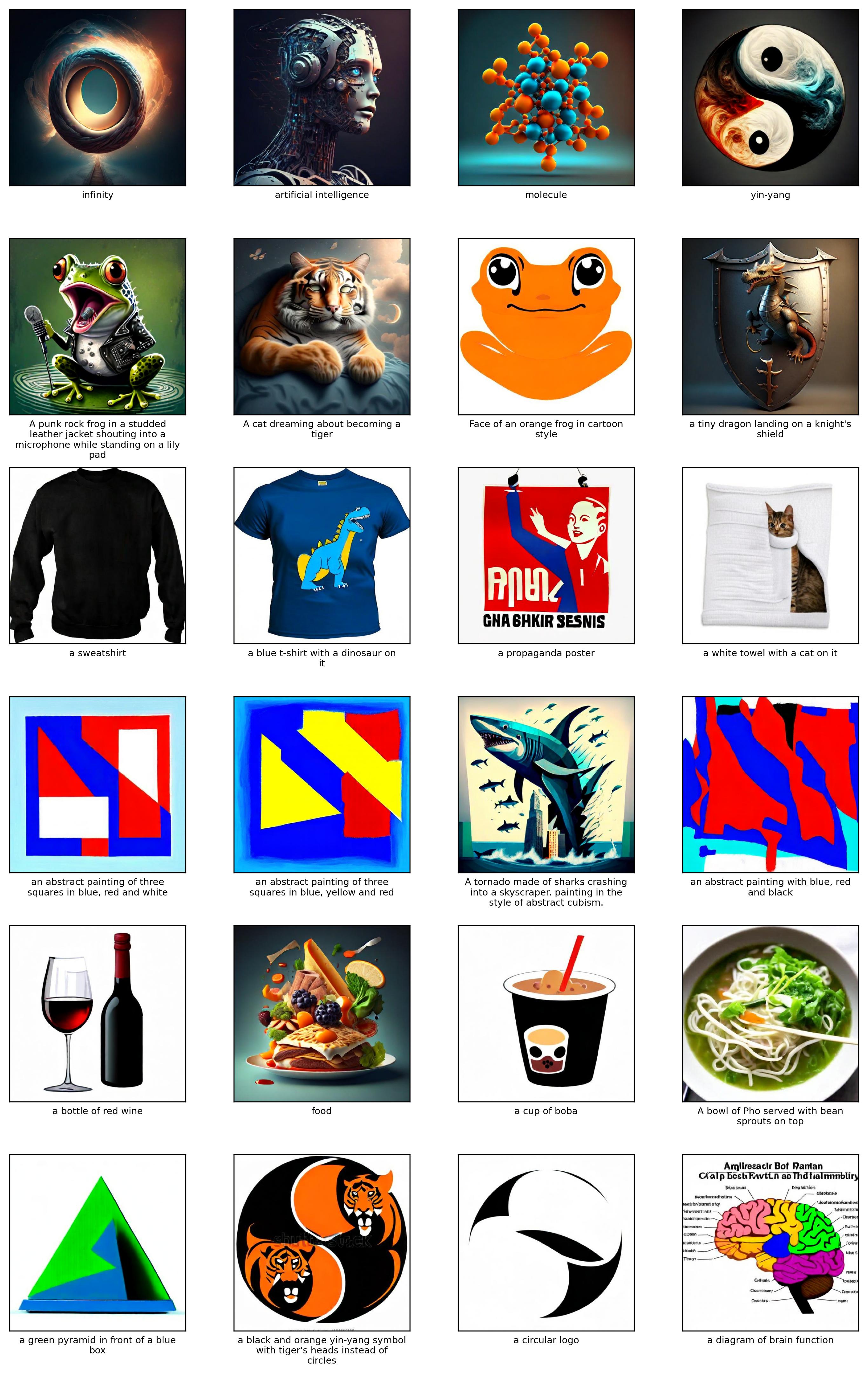
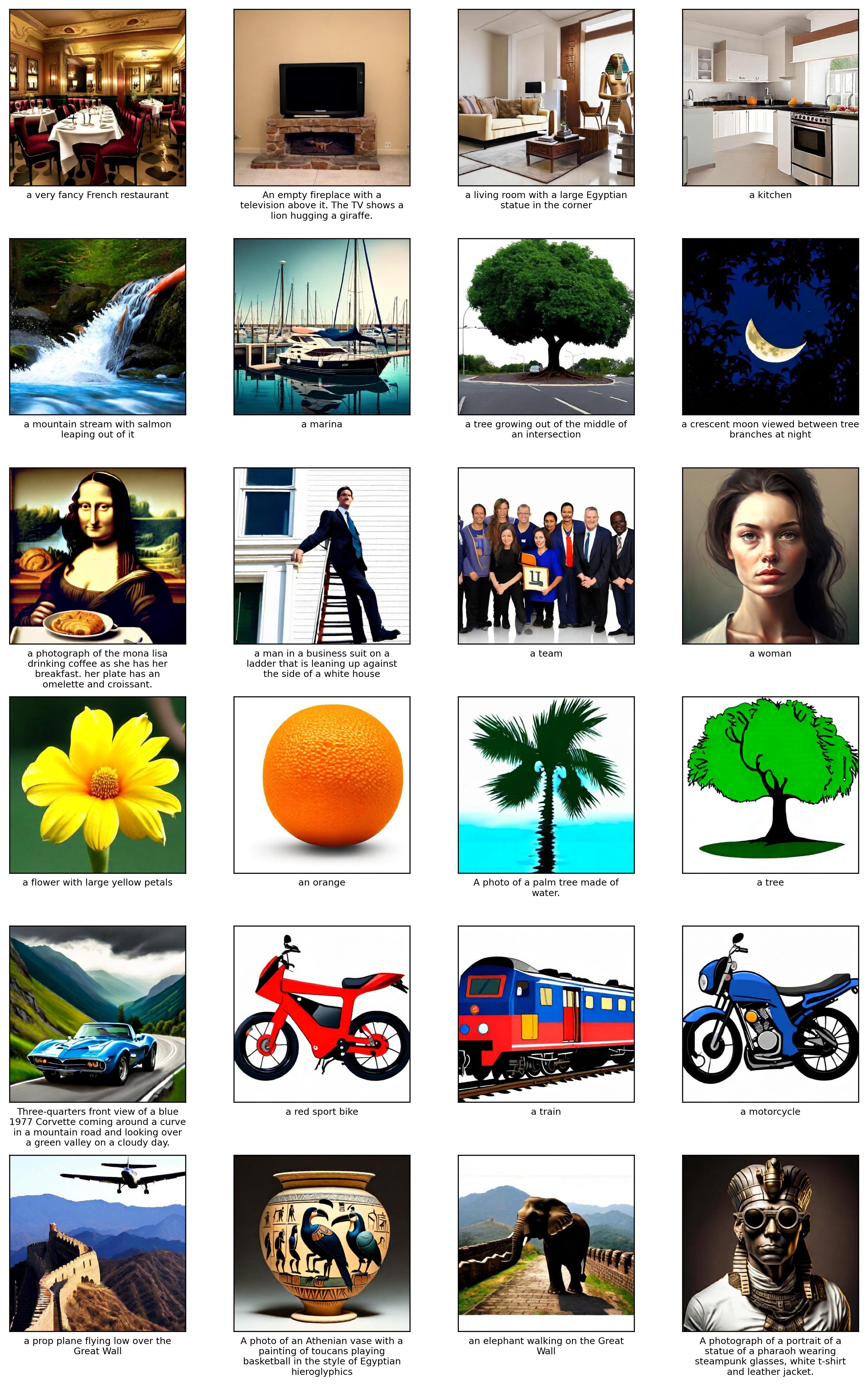
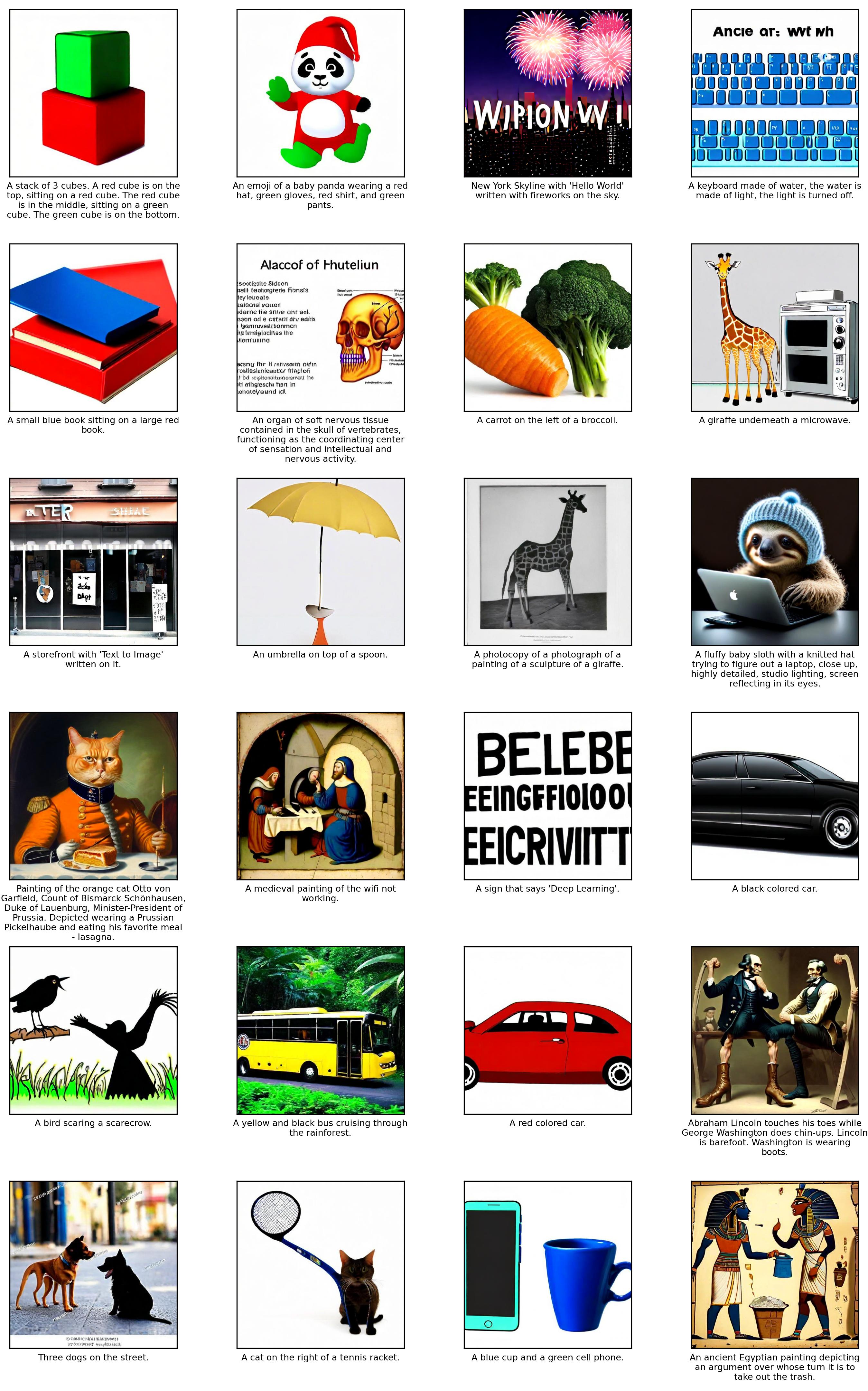
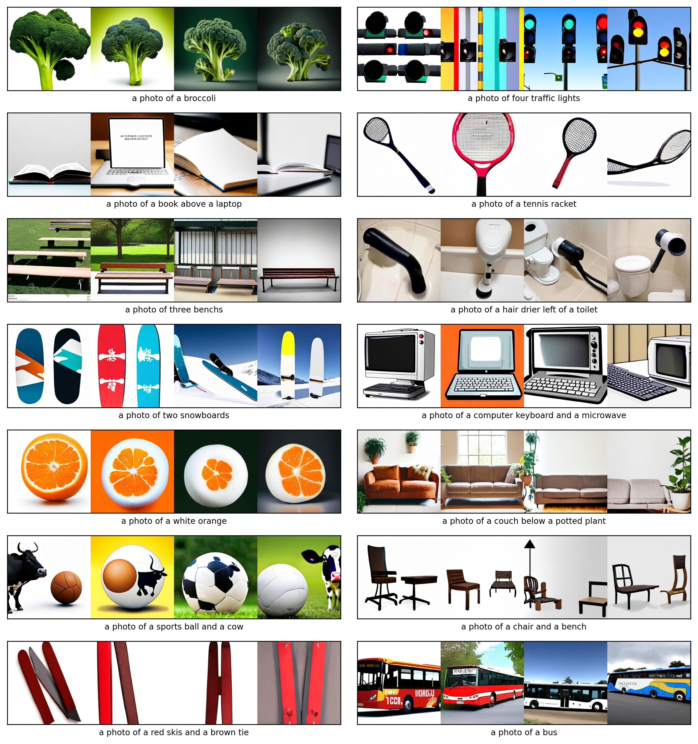
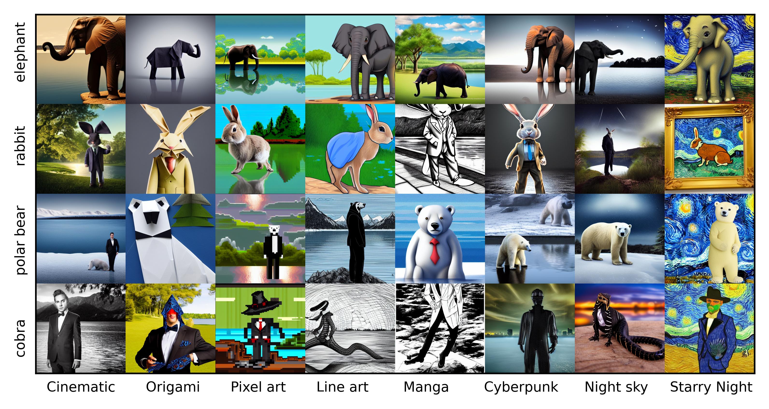
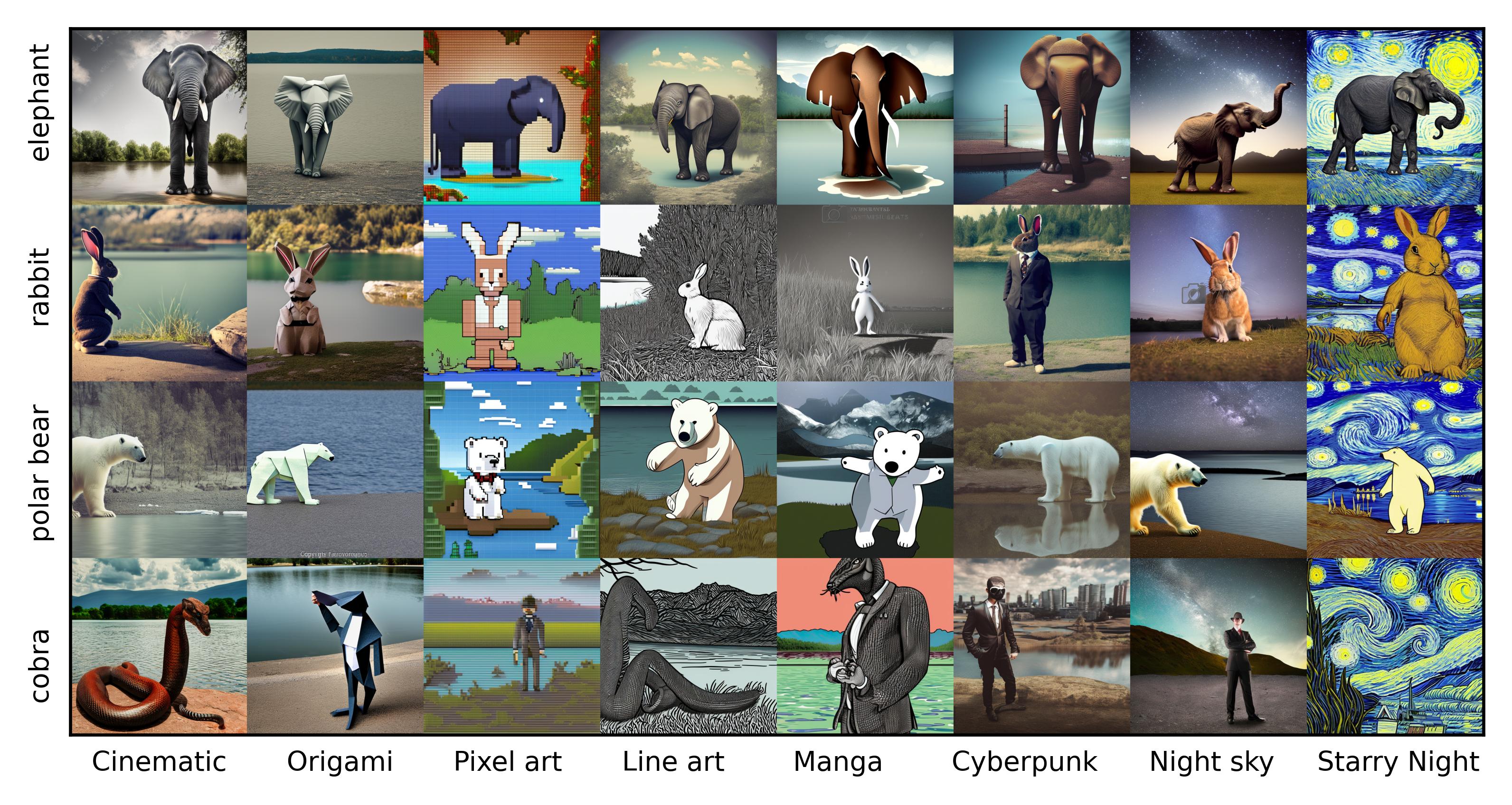
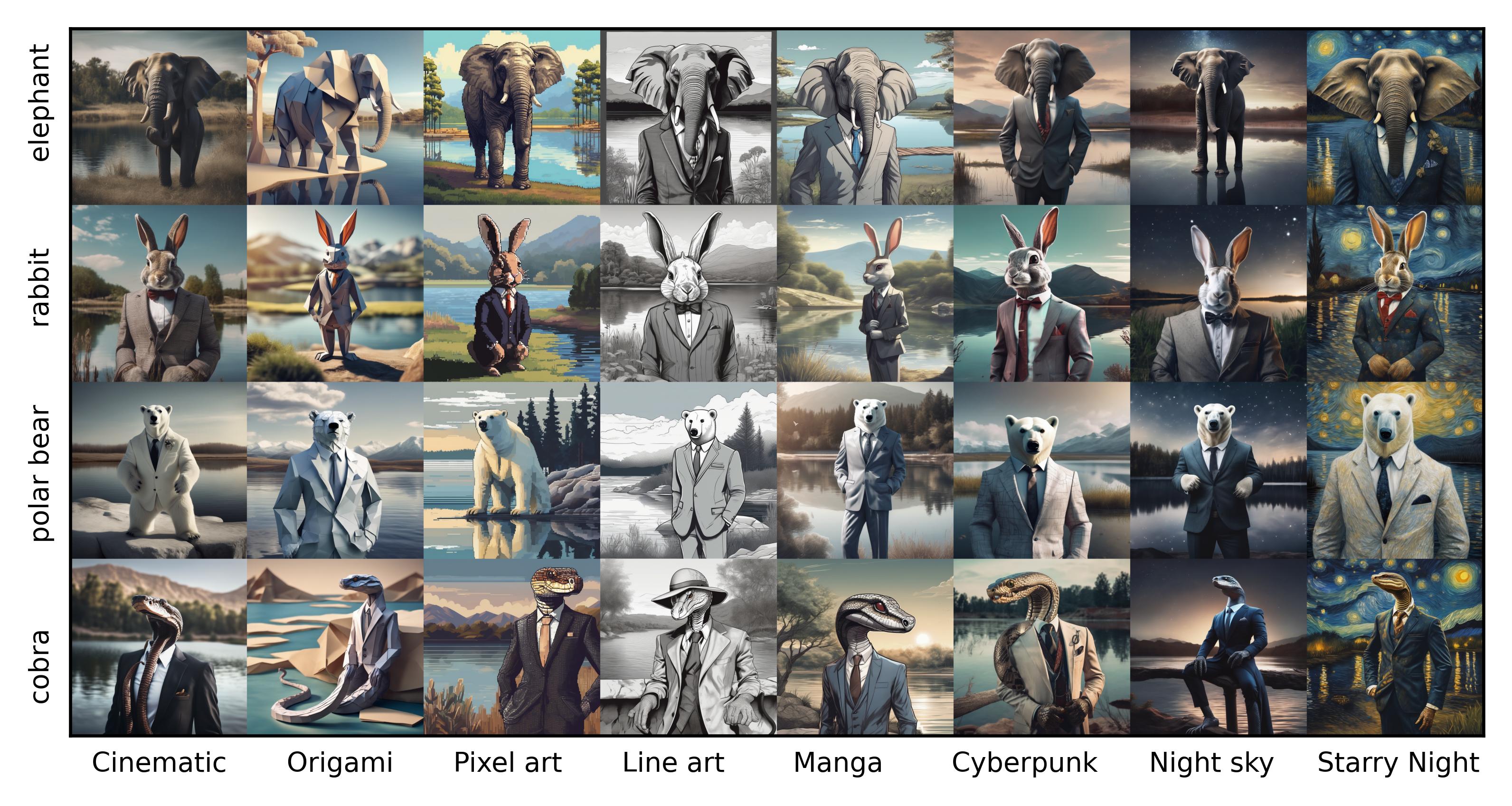
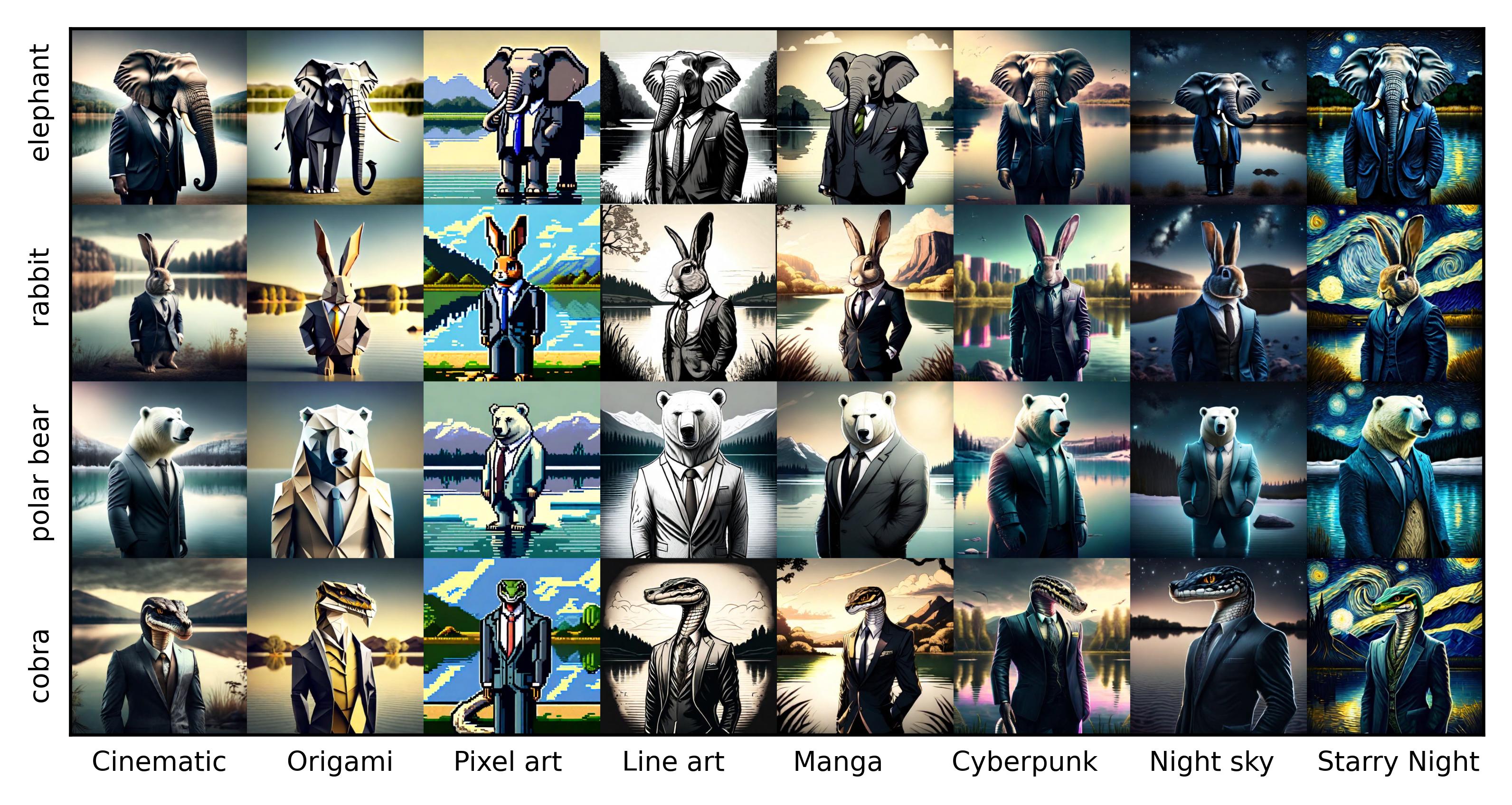
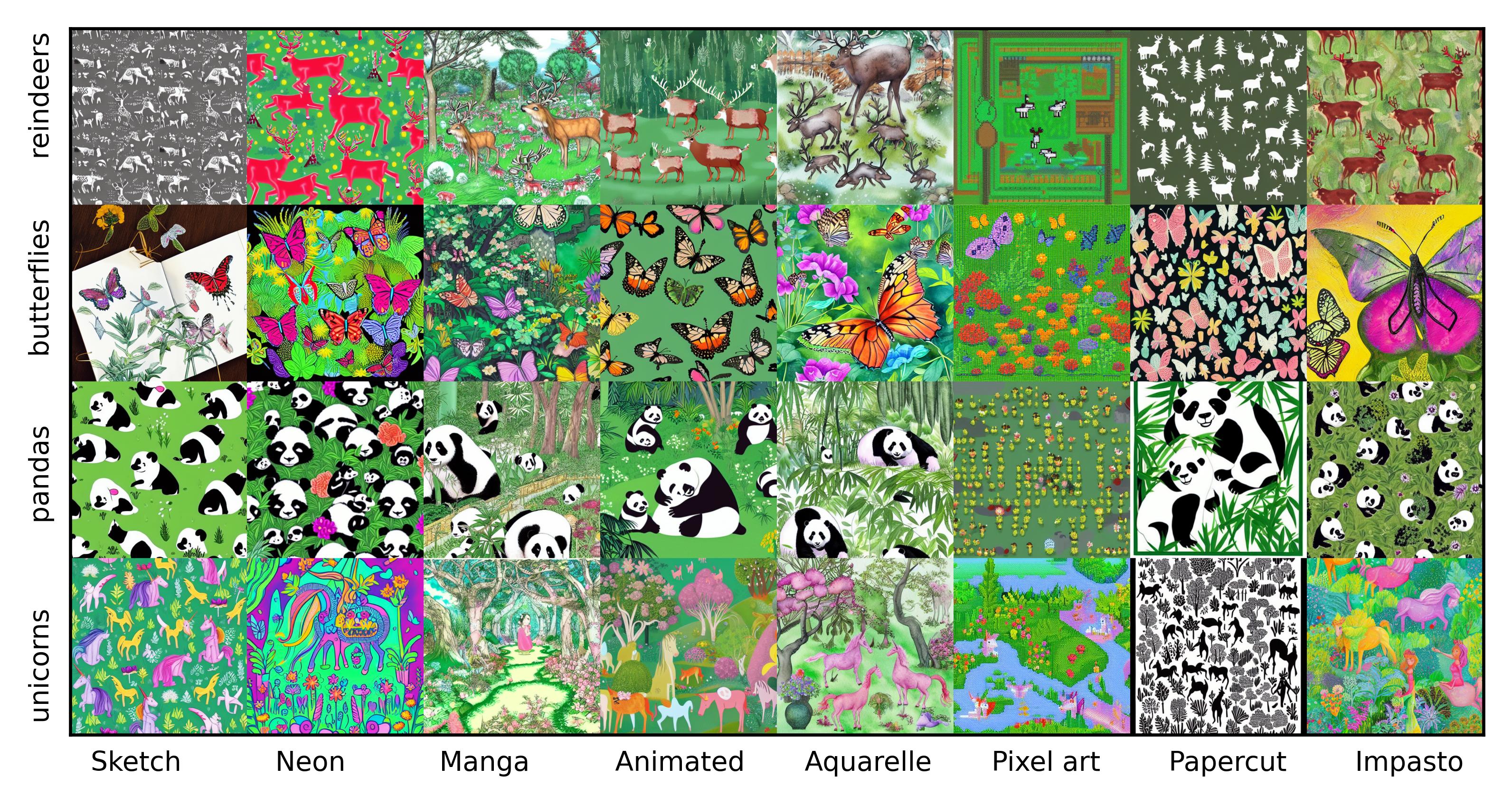
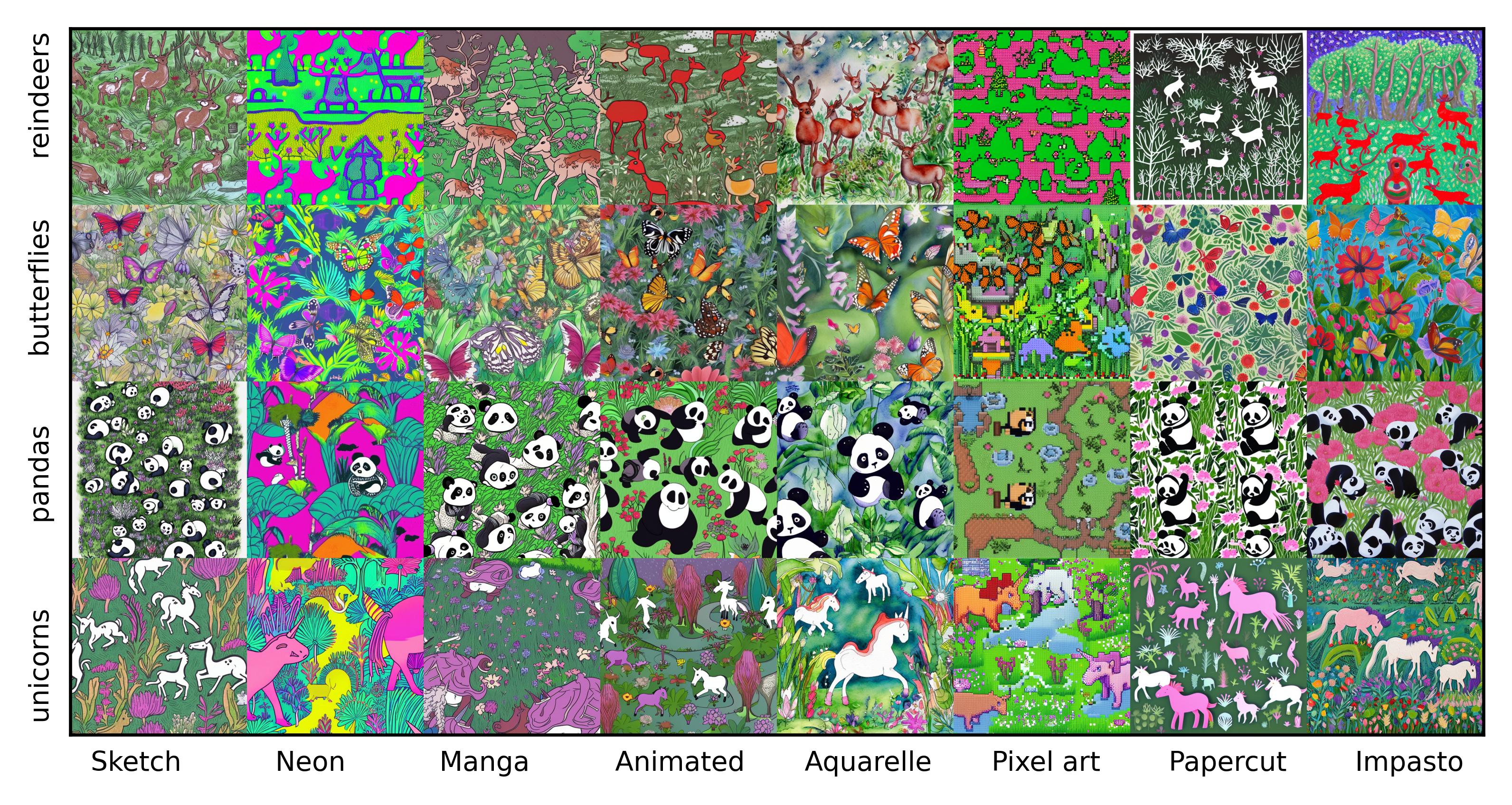
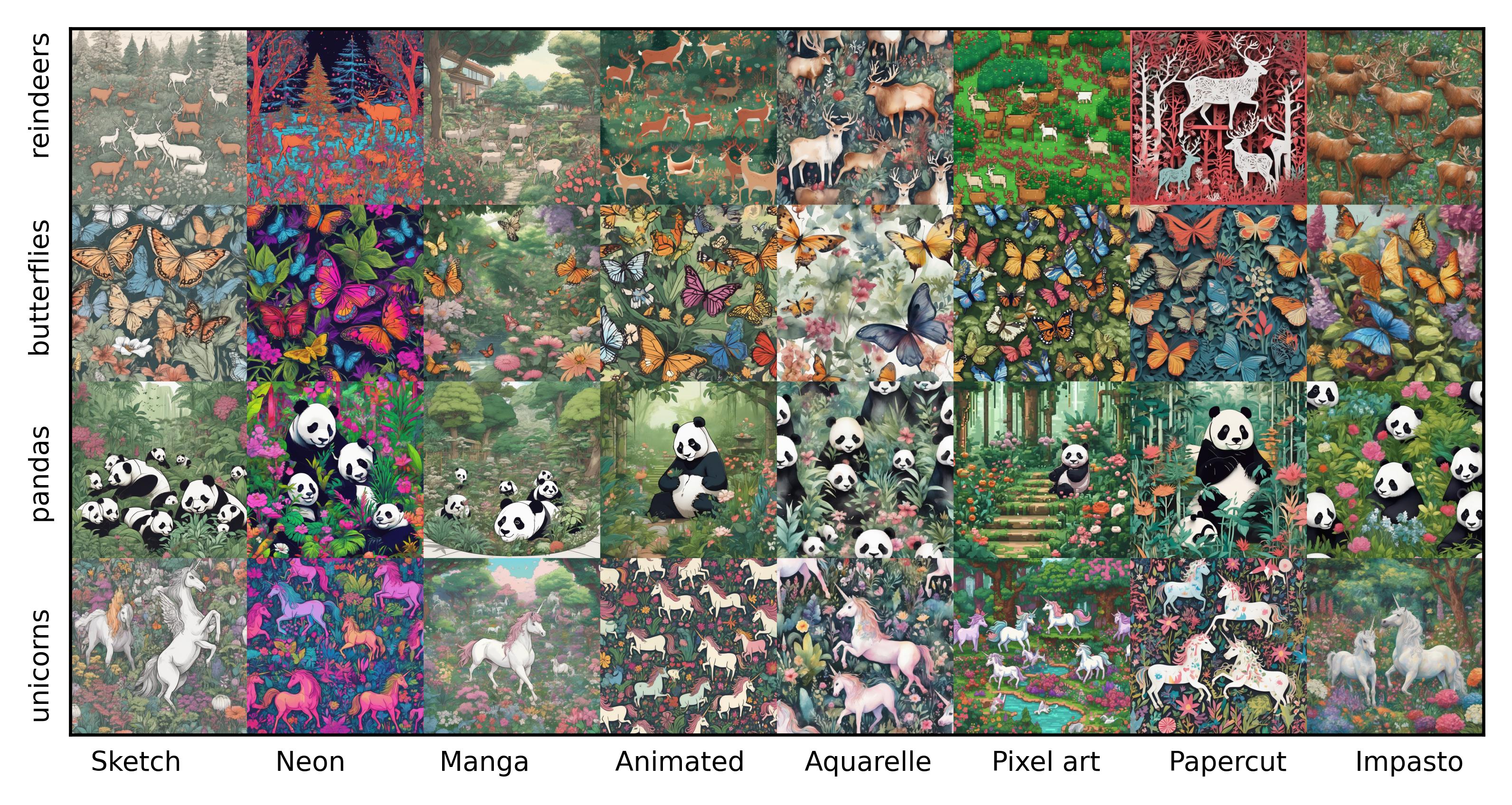
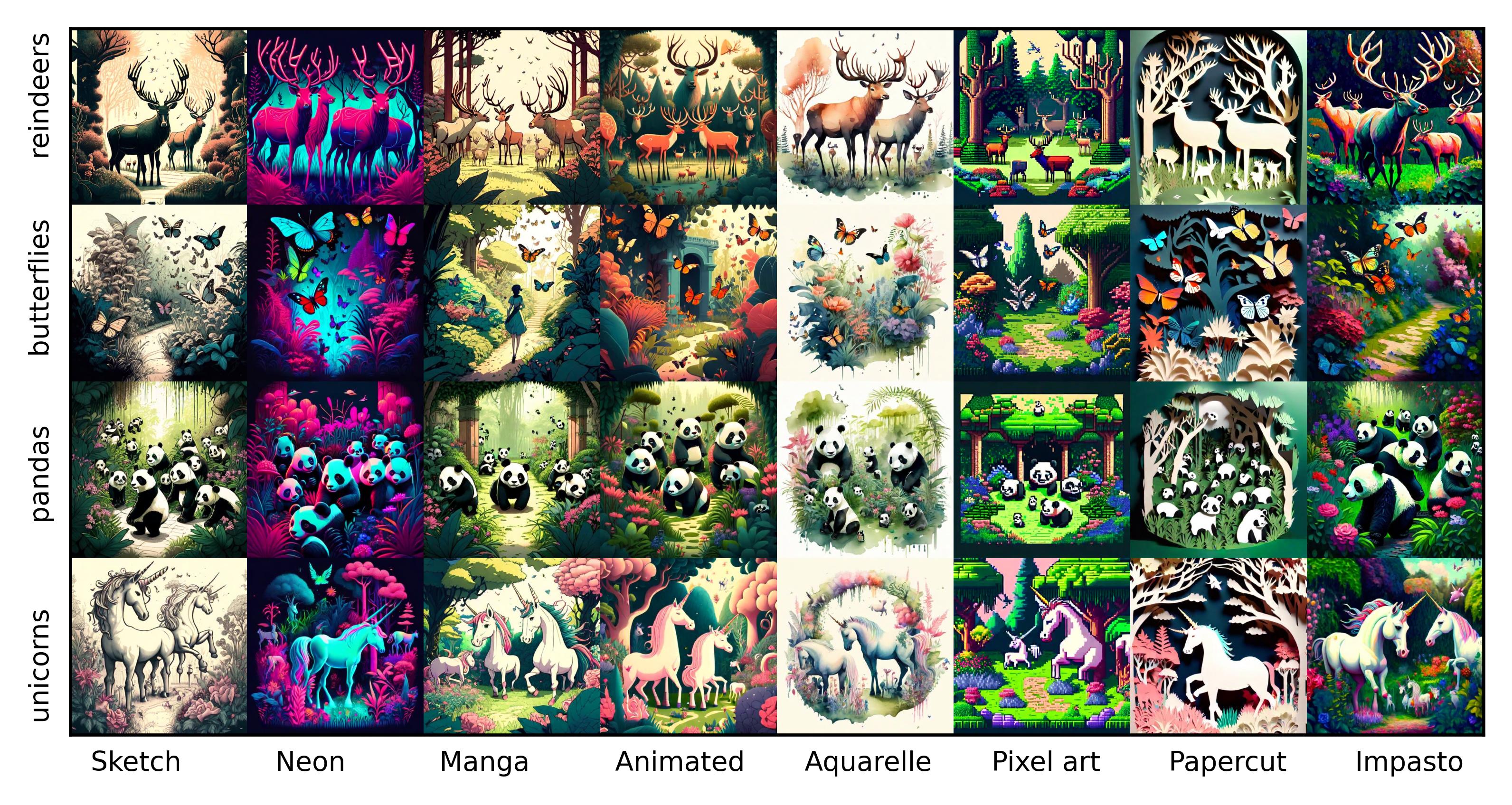
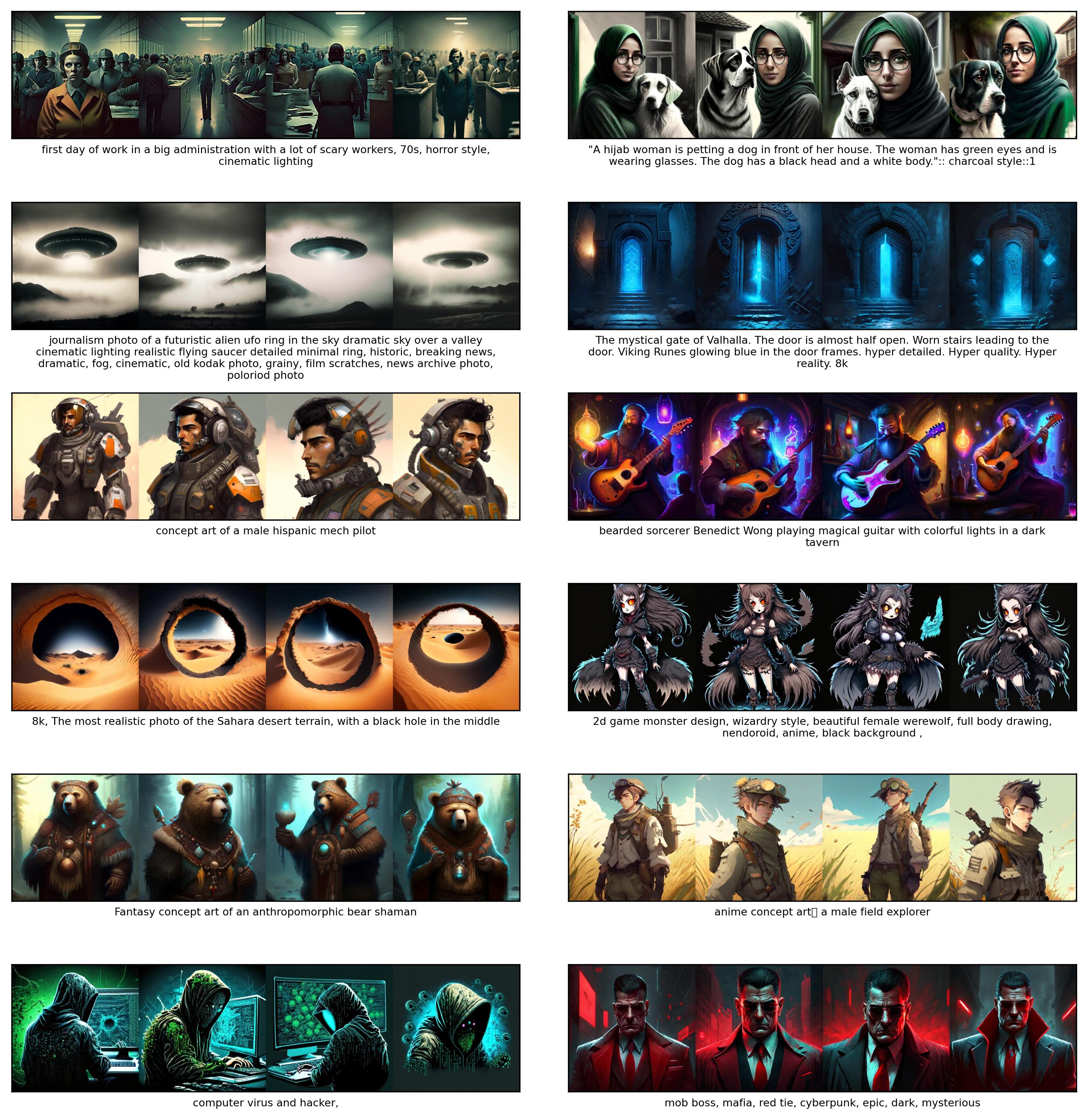
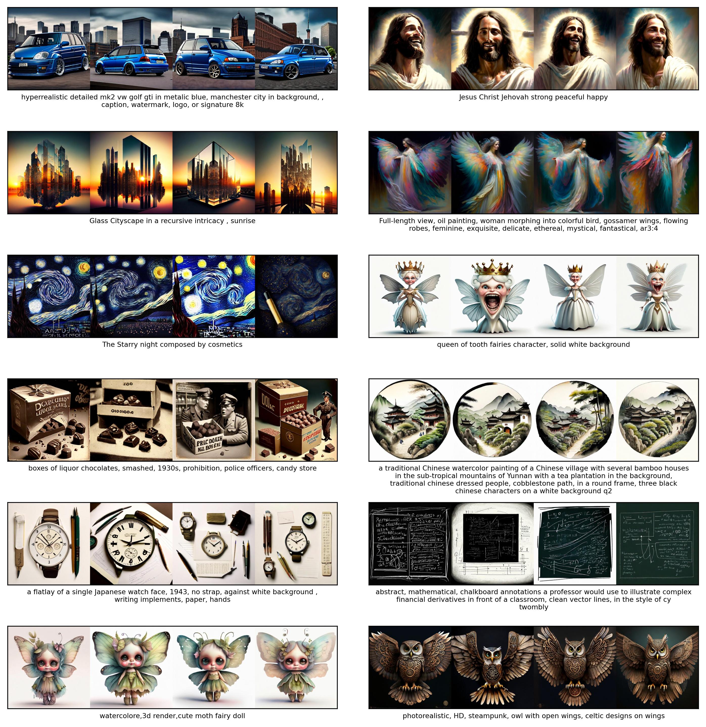
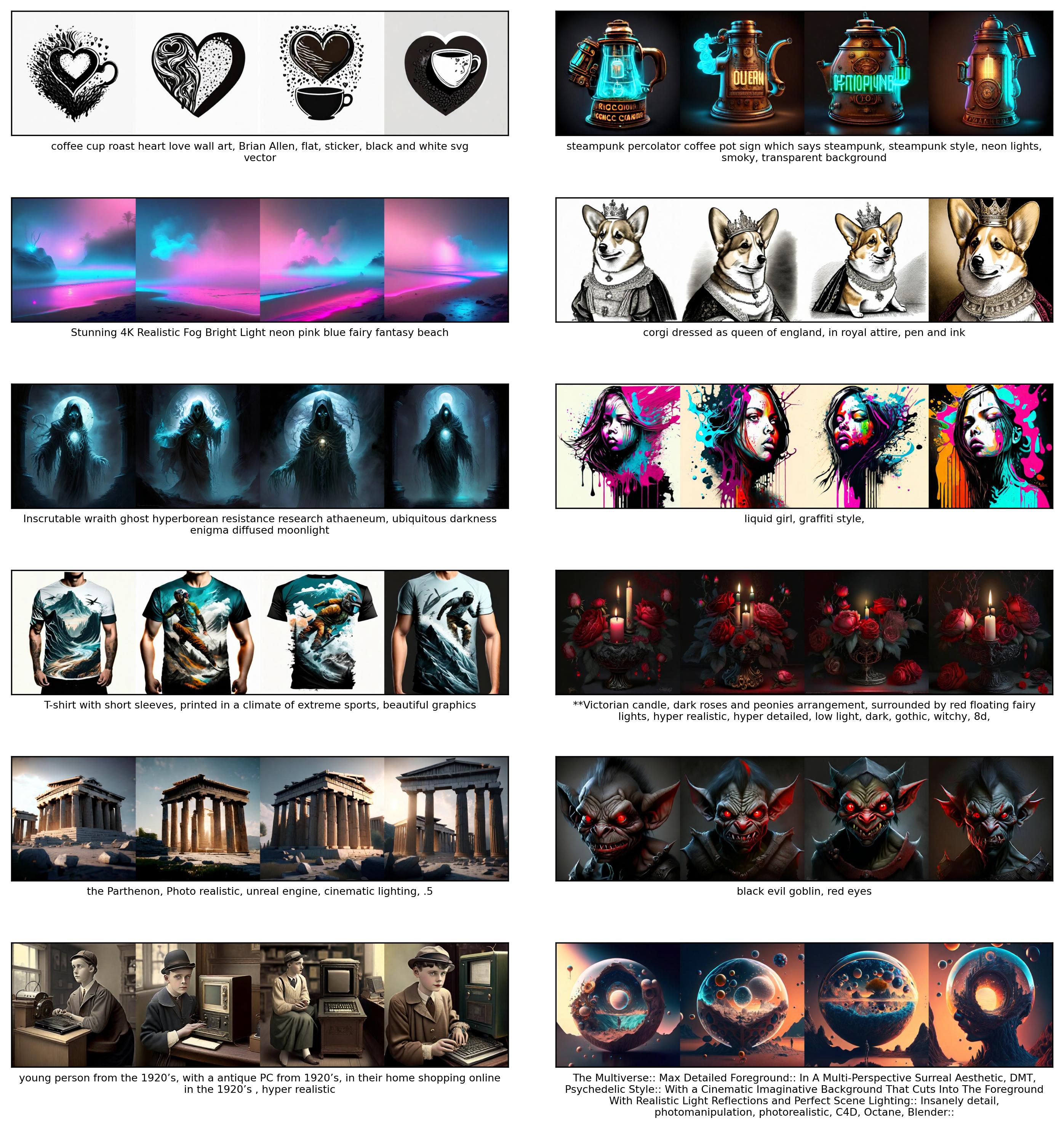
Stretching Each Dollar: Diffusion Training from Scratch on a Micro-Budget

Abstract

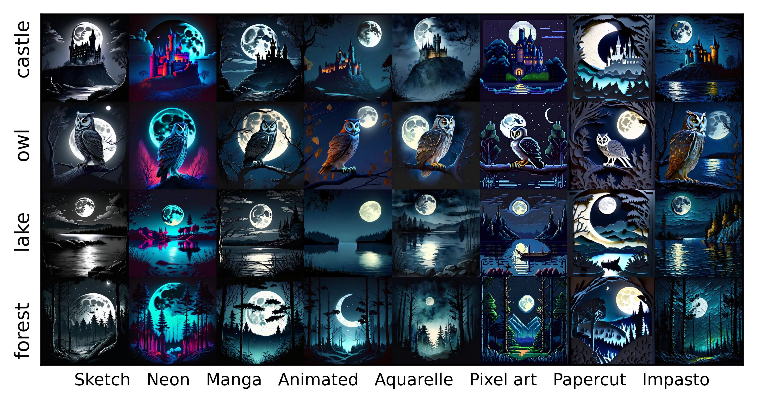
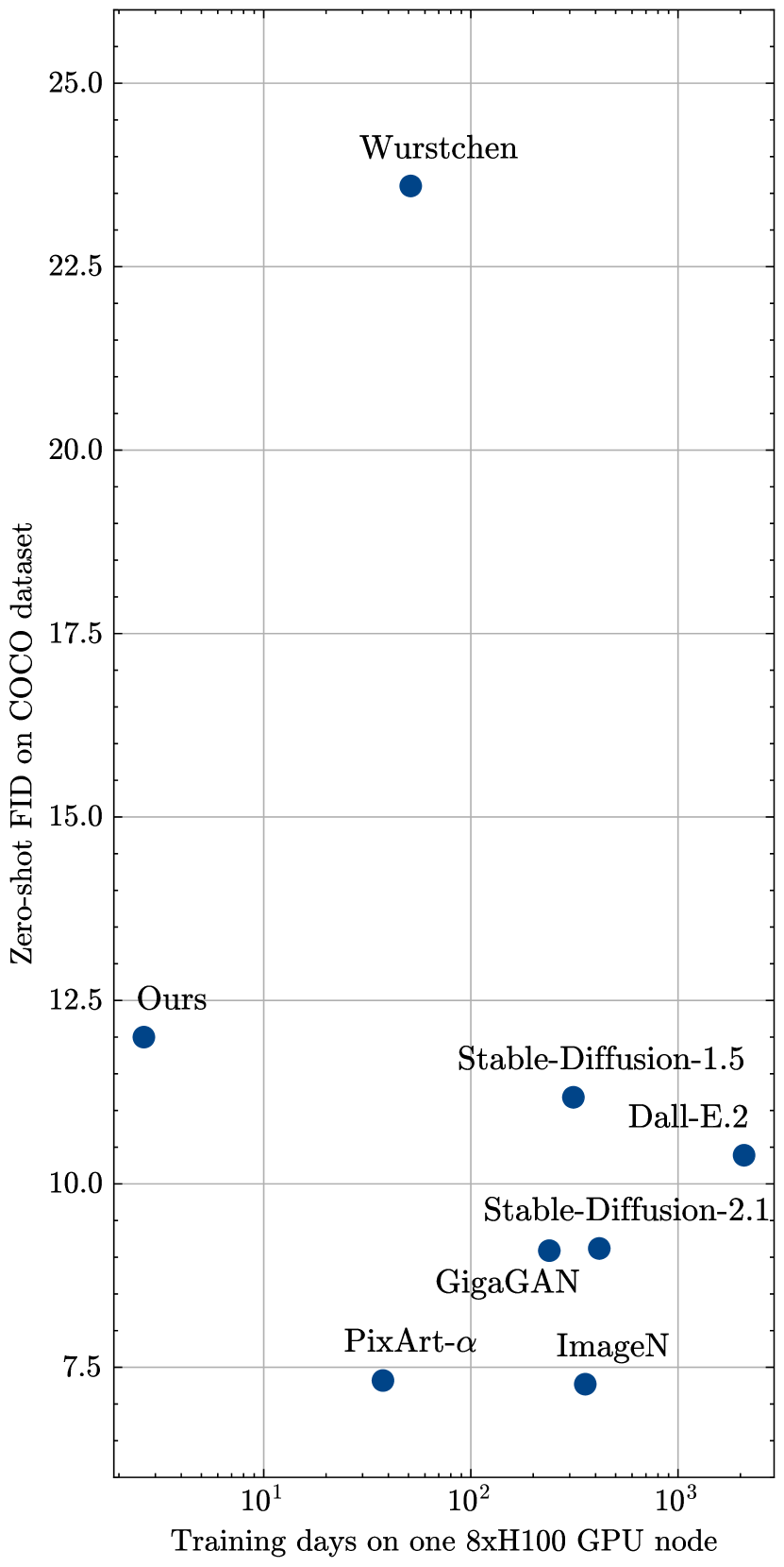
As scaling laws in generative AI push performance, they also simultaneously concentrate the development of these models among actors with large computational resources. With a focus on text-to-image (T2I) generative models, we aim to address this bottleneck by demonstrating very low-cost training of large-scale T2I diffusion transformer models. As the computational cost of transformers increases with the number of patches in each image, we propose to randomly mask up to 75% of the image patches during training. We propose a deferred masking strategy that preprocesses all patches using a patch-mixer before masking, thus significantly reducing the performance degradation with masking, making it superior to model downscaling in reducing computational cost. We also incorporate the latest improvements in transformer architecture, such as the use of mixture-of-experts layers, to improve performance and further identify the critical benefit of using synthetic images in micro-budget training. Finally, using only 37M publicly available real and synthetic images, we train a 1.16 billion parameter sparse transformer with only $1,890 economical cost and achieve a 12.7 FID in zero-shot generation on the COCO dataset. Notably, our model achieves competitive FID and high-quality generations while incurring 118$\times$ lower cost than stable diffusion models and 14$\times$ lower cost than the current state-of-the-art approach that costs $28,400. We aim to release our end-to-end training pipeline to further democratize the training of large-scale diffusion models on micro-budgets.

¹ Sony AI, ² University of California, Riverside

An elegant squirrel pirate on a ship.; A hippo in a ballet performance in a white swan dress; A photo realistic koala bear playing a guitar; A rabbit magician pulling a hat.

A real life samurai standing in a green bamboo grove; A fairy tale castle in the clouds; A real looking vibrant butterfly on a photorealistic flower; A mystical cave with glowing crystals.

A cute rabbit in a stunning, detailed chinese coat; A frog on a lotus leaf.; Toy elephants made of Mahogany wood on a shelf; A logo of a fox in neon light.

Ancient castle of a cliff edge; Serene beach with colourful pebble stones; Photo realistic market place in a medieval town; Alien landscape with two moons.

A realistic train made of origami.; A soccer plaground made of snow and timber.; Pre war apartment complexes reflected in the water of a beautifull lake.; A wolf coming out of the woods.

A dolphin astronaut in space in astronaut suit; Kangaroo boxing champions on a mountain top; A photo realistic turtle reading a book using a table lamp; A realistic penguin detective with magnifying glass in a crime scene.

A four layer wedding cake; A cactus smiling in a desert; Miniature cat made of lego playing with other cats in a room; An adorable baby dinosaur dressed as cowboy on a beach

Mountain covered in snow; A cat wearing a wizard hat; A train made of realistic pumpkins; A robot on a blue planet. Close up shot.                                                                                                                                                                                                                                                                                                              

(a) Stable-Diffusion-1.5

(b) Stable-Diffusion-2.1

(c) Ours

(d) FID vs. training time

Figure 1: Qualitative evaluation of the image generation capabilities of our model ($512\times 512$ image resolution) . Our model is trained in $2.6$ days on a single 8$\times$H100 machine (amounting to only $1,890 in GPU cost) without any proprietary or billion image dataset. In (a)-(c) we examine diverse style generation capabilities using prompt ‘Image of an astronaut riding a horse in   style’, with following styles: Origami, Pixel art, Line art, Cyberpunk, and Van Gogh Starry Night. In (d) we compare training cost and fidelity, measured using FID (Heusel et al., 2017) for zero-shot image generation on COCO (Lin et al., 2014) dataset, of all models.

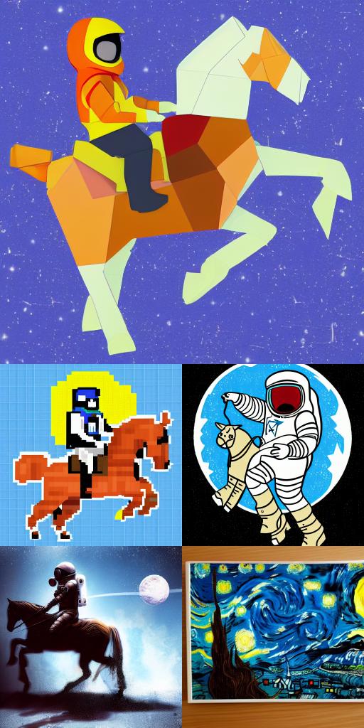
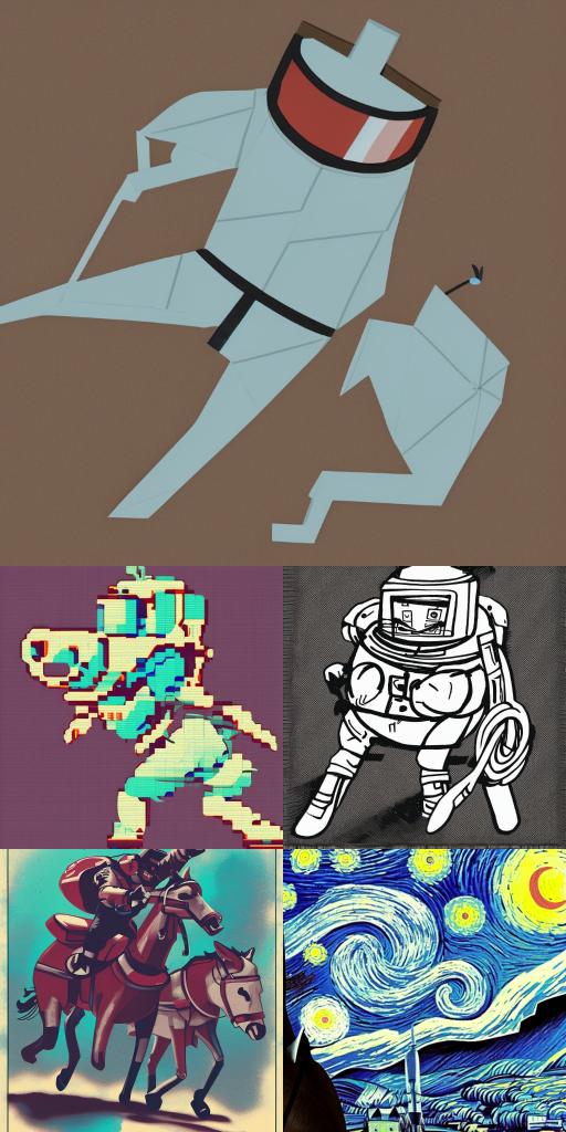
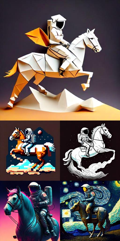
1 Introduction

While modern visual generative models excel at creating photorealistic visual content and have propelled the generation of more than a billion images each year (Valyaeva, 2023), the cost and effort of training these models from scratch remain very high (Rombach et al., 2022; Ramesh et al., 2022; Saharia et al., 2022). In text-to-image diffusion models (T2I) (Song et al., 2020a; Ho et al., 2020; Song et al., 2021), some previous works have successfully scaled down the computational cost compared to the 200,000 A100 GPU hours used by Stable Diffusion 2.1 (Rombach et al., 2022; Chen et al., 2023; Pernias et al., 2024; Gokaslan et al., 2024). However, the computational cost of even the state-of-the-art approaches (18,000 A100 GPU hours) remains very high (Chen et al., 2023), requiring more than a month of training time on the leading 8$\times$H100 GPU machine. Furthermore, previous works either leverage larger-scale datasets spanning on the order of a billion images or use proprietary datasets to enhance performance (Rombach et al., 2022; Chen et al., 2023; Yu et al., 2022; Saharia et al., 2022). The high training cost and the dataset requirements create an inaccessible barrier to participating in the development of large-scale diffusion models. In this work, we aim to address this issue by developing a low-cost end-to-end pipeline for competitive text-to-image diffusion models that achieve more than an order of magnitude reduction in training cost than the state-of-the-art while not requiring access to billions of training images or proprietary datasets.

We consider vision transformer based latent diffusion models for text-to-image generation (Dosovitskiy et al., 2020; Peebles & Xie, 2023), particularly because of their simplified design and wide adoption across the latest large-scale diffusion models (Betker et al., 2023; Esser et al., 2024; Chen et al., 2023). To reduce the computational cost, we exploit the strong dependence of the transformer’s computational cost on the input sequence size, i.e., the number of patches per image. We aim to reduce the effective number of patches processed per image by the transformer during training. This objective can be easily achieved by randomly masking a fraction of the tokens at the input layer of the transformer. However, existing masking approaches fail to scale beyond a 50% masking ratio without drastically degrading performance (Zheng et al., 2024), particularly because, at high masking ratios, a large fraction of input patches are completely unobserved by the diffusion transformer.

To mitigate the massive performance degradation with masking, we propose a deferred masking strategy where all patches are preprocessed by a lightweight patch-mixer before being transferred to the diffusion transformer. The patch mixer comprises a fraction of the number of parameters in the diffusion transformer. In contrast to naive masking, masking after patch mixing allows non-masked patches to retain semantic information about the whole image and enables reliable training of diffusion transformers at very high masking ratios, while incurring no additional computational cost compared to existing state-of-the-art masking (Zheng et al., 2024). We also demonstrate that under an identical computational budget, our deferred masking strategy achieves better performance than model downscaling, i.e., reducing the size of the model. Finally, we incorporate recent advancements in transformer architecture, such as layer-wise scaling (Mehta et al., 2024) and sparse transformers using mixture-of-experts (Shazeer et al., 2017; Zoph et al., 2022; Zhou et al., 2022), to improve performance in large-scale training.

Our low-cost training pipeline naturally reduces the overhead of ablating experimental design choices at scale. One such ablation we run is examining the impact of the choice of training datasets on the performance of micro-budget training. In addition to using only real images, we consider combining additional synthetic images in the training dataset. We find that training on a combined dataset significantly improves image quality and alignment with human visual preferences. Furthermore, our combined dataset comprises only 37M images, significantly fewer than most existing large-scale models, thus providing strong evidence of high-quality generations from moderate-sized datasets in micro-budget training.

In summary, we make the following key contributions.

• We propose a novel deferred patch masking strategy that preprocesses all patches before masking by appending a lightweight patch-mixer model to the diffusion transformer.

• We conduct extensive ablations of deferred masking and demonstrate that it enables reliable training at high masking ratios and achieves significantly better performance compared to alternatives such as other masking strategies and model downscaling.

• We demonstrate that rather than limiting to only real image datasets, combining additional synthetic images in micro-budget training significantly improves the quality of generated images.

• Using a micro-budget of only $1,890, we train a 1.16 billion parameter sparse diffusion transformer on 37M images and a 75% masking ratio that achieves a 12.7 FID in zero-shot generation on the COCO dataset. The wall-clock time of our training is only 2.6 days on a single $8\times$H100 GPU machine, 14$\times$ lower than the current state-of-the-art approach that would take 37.6 training days ($28,400 GPU cost).

2 Methodology

In this section, we first provide a background on diffusion models, followed by a review of common approaches, particularly those based on patch masking, to reduce computational costs in training diffusion transformers. Then, we provide a detailed description of our proposed deferred patch masking strategy.

2.1 Background: Diffusion-based generative models and diffusion transformers

We denote the data distribution by $\mathcal{D}$, such that $({\boldsymbol{x}},{\boldsymbol{c}})\sim\mathcal{D}$, where ${\boldsymbol{x}}$ and ${\boldsymbol{c}}$ represent the image and the corresponding natural language caption, respectively. We assume that $p({\boldsymbol{x}};\sigma)$ is the image distribution obtained after adding $\sigma^{2}$-variance Gaussian noise.

Diffusion-based probabilistic models use a forward-reverse process-based approach, where the forward process corrupts the input data and the reverse process tries to reconstruct the original signal by learning to reconstruct the data degradation at each step. Though multiple variations of diffusion models exists (Ho et al., 2020; Song et al., 2020b; Bansal et al., 2024), it is common to use time-dependent Gaussian noise ($\sigma(t)$) for model data corruption. Under deterministic sampling, both the forward and reverse processes in diffusion models can be modeled using an ordinary differential equation (ODE).

$$\text{d}{\boldsymbol{x}}=-\dot{\sigma}(t)\sigma(t)\nabla_{\boldsymbol{x}}\log p({\boldsymbol{x}};\sigma(t))\text{d}t,$$ (1)

where $\dot{\sigma}(t)$ represents the time derivative and $\nabla_{\boldsymbol{x}}\log p({\boldsymbol{x}};\sigma(t))$ is the score of the underlying density function. Thus the move towards (or away from) higher density regions in the diffusion process is proportional to both the scores of the density function and changes in the noise distribution ($\sigma(t)$) with time. Going beyond the deterministic sampling based on the ODE formulation in Equation 1, the sampling process in diffusion models can also be formulated as a stochastic differential equation,

$$\text{d}{\boldsymbol{x}}=\underbrace{-\dot{\sigma}(t)\sigma(t)\nabla_{\boldsymbol{x}}\log p({\boldsymbol{x}};\sigma(t))\text{d}t}_{\text{Probability flow ODE (Eq.~{}\ref{eq: score-ode})}}-\underbrace{\beta(t)\sigma(t)^{2}\nabla_{\boldsymbol{x}}\log p({\boldsymbol{x}};\sigma(t))\text{d}t}_{\text{Deterministic noise decay}}+\underbrace{\sqrt{2\beta(t)}\sigma(t)}_{\text{Noise injection}}\text{d}w_{t}$$ (2)

where $\text{d}w_{t}$ is standard the Wiener process and the parameter $\beta(t)$ controls the rate of injection of additional noise. The generation process in diffusion models starts by sampling an instance from $p({\boldsymbol{x}},\sigma_{\text{max}})$ and iteratively denoising it using the ODE or SDE-based formulation.

Training. Diffusion model training is based on parameterizing the score of the density function, which doesn’t depend on the generally intractable normalization factor, using a denoiser, i.e., $\nabla_{\boldsymbol{x}}\log p({\boldsymbol{x}};\sigma(t))\approx\left(F_{\theta}({\boldsymbol{x}},\sigma(t))-{\boldsymbol{x}}\right)/\sigma(t)^{2}$. The denoising function $F_{\theta}({\boldsymbol{x}},\sigma(t))$ is generally modeled using a deep neural network. For text-to-image generation, the denoiser is conditioned on both noise distribution and natural language captions and trained using the following loss function,

$$\mathcal{L}=\mathbb{E}_{({\boldsymbol{x}},{\boldsymbol{c}})\sim\mathcal{D}}\mathbb{E}_{{\boldsymbol{\epsilon}}\sim\mathcal{N}(\boldsymbol{0},\sigma(t)^{2}\mathbf{I})}\|F_{\theta}({\boldsymbol{x}}+{\boldsymbol{\epsilon}};\sigma(t),{\boldsymbol{c}})-{\boldsymbol{x}}\|_{2}^{2}.$$ (3)

The noise distribution during training is lognormal ($\text{ln}(\sigma)\sim\mathcal{N}(P_{\text{mean}},P_{\text{std}})$), where the choice of the mean and standard deviation of the noise distribution strongly influences the quality of generated samples. For example, the noise distribution is shifted to the right to sample larger noise values on higher resolution images, as the signal-to-noise ratio increases with resolution (Teng et al., 2023).

Classifier-free guidance. To increase alignment between input captions and generated images, classifier-free guidance (Ho & Salimans, 2022) modifies the image denoiser to output a linear combination of denoised samples in the presence and absence of input captions.

$$\hat{F}_{\theta}({\boldsymbol{x}};\sigma(t),{\boldsymbol{c}})=F_{\theta}({\boldsymbol{x}};\sigma(t))+w\cdot(F_{\theta}({\boldsymbol{x}};\sigma(t),{\boldsymbol{c}})-F_{\theta}({\boldsymbol{x}};\sigma(t))),$$ (4)

where $w\geq 1$ controls the strength of guidance. During training, a fraction of image captions (commonly set to 10%) are randomly dropped to learn unconditional generation.

Latent diffusion models. In contrast to modeling higher dimensional pixel space ($\mathbb{R}^{h\times w\times 3}$), latent diffusion models (Rombach et al., 2022) are trained in a much lower dimensional compressed latent space ($\mathbb{R}^{\frac{h}{n}\times\frac{w}{n}\times c}$), where $n$ is the compression factor and $c$ is the number of channels in the latent space. The image-to-latent encoding and its reverse mapping are performed by a variational autoencoder. Latent diffusion models achieve faster convergence than training in pixel space and have been heavily adopted in large-scale diffusion models (Podell et al., 2024; Betker et al., 2023; Chen et al., 2023; Balaji et al., 2022).

Diffusion transformers. We consider that the transformer model ($F_{\theta}$) consists of $k$ hierarchically stacked transformer blocks. Each block consists of a multi-head self-attention layer, a multi-head cross-attention layer, and a feed-forward layer. For simplicity, we assume that all images are converted to a sequence of patches to be compatible with the transformer architecture. In the transformer architecture, we refer to the width of all linear layers as $d$.

2.2 Common approaches towards minimizing the computational cost of training diffusion transformers

Assuming transformer architectures where linear layers account for the majority of the computational cost, the total training cost is proportional to $M\times N\times S$, where $M$ is the number of samples processed, $N$ is the number of model parameters, and $S$ is the number of patches derived from one image, i.e., sequence size for transformer input (Figure 2a). As our goal is to train an open-world model, we believe that a large number of parameters are required to support diverse concepts during generation; thus, we opt to not decrease the parameter count significantly. Since diffusion models converge slowly and are often trained for a large number of steps, even for small-scale datasets, we keep this choice intact (Rombach et al., 2022; Balaji et al., 2022). Instead, we aim to exploit any redundancy in the input sequence to reduce computational cost while simultaneously not drastically degrade performance.

A. Using larger patch size (Figure 2b). In a vision transformer, the input image is first transformed into a sequence of non-overlapping patches with resolution $p\times p$, where $p$ is the patch size (Dosovitskiy et al., 2020). Though using a higher patch size quadratically reduces the number of patches per image, it can significantly degrade performance due to the aggressive compression of larger regions of the image into a single patch.

B. Using patch masking (Figure 2c). A contemporary approach is to keep the patch size intact but drop a large fraction of patches at the input layer of the transformer (He et al., 2022). Naive token masking is similar to training on random crops in convolutional UNets, where often upsampling diffusion models are trained on smaller random crops rather than the full image (Nichol et al., 2021; Saharia et al., 2022). However, in contrast to random crops of the images, patch masking allows training on non-continuous regions of the image. Due to its effectiveness, masking-based training of transformers has been adopted across both vision and language domains (Devlin et al., 2018; He et al., 2022).

C. Masking patches with autoencoding (MaskDiT - Figure 2d). In order to also encourage representation learning from masked patches, Zheng et al. (2024) adds an auxiliary autoencoding loss that encourages the reconstruction of masked patches. This formulation was motivated by the success of the autoencoding loss in learning self-supervised representations (He et al., 2022). MaskDiT first appends a lightweight decoder, a small-scale transformer network, to the larger backbone transformer. Before the decoder, it expands the backbone transformer output by inserting spurious learnable patches in place of masked patches.

Assuming that the binary mask $m$ represents the masked patches, the final training loss is the following,

$$\mathcal{L}_{\text{diff}}=\mathbb{E}_{({\boldsymbol{x}},{\boldsymbol{c}})\sim\mathcal{D}}\mathbb{E}_{{\boldsymbol{\epsilon}}\sim\mathcal{N}(\boldsymbol{0},\sigma(t)^{2}\mathbf{I})}\|\left(\bar{F}_{\theta}(({\boldsymbol{x}}+{\boldsymbol{\epsilon}})\odot(1-m);\sigma,{\boldsymbol{c}})-{\boldsymbol{x}}\right)\odot(1-m)\|_{2}^{2}$$ (5)

$$\mathcal{L}_{\text{mae}}=\mathbb{E}_{({\boldsymbol{x}},{\boldsymbol{c}})\sim\mathcal{D}}\mathbb{E}_{{\boldsymbol{\epsilon}}\sim\mathcal{N}(\boldsymbol{0},\sigma(t)^{2}\mathbf{I})}\|\left(\bar{F}_{\theta}(({\boldsymbol{x}}+{\boldsymbol{\epsilon}})\odot(1-m);\sigma,{\boldsymbol{c}})-({\boldsymbol{x}}+{\boldsymbol{\epsilon}})\right)\odot m\|_{2}^{2}$$ (6)

$$\mathcal{L}=\mathcal{L}_{\text{diff}}+\gamma\mathcal{L}_{\text{mae}}$$ (7)

where $\bar{F}_{\theta}$ represents the sequential backbone transformer and decoder module, and $\gamma$ is a hyperparameter to balance the influence of the masked autoencoding loss with respect to the diffusion training loss.

Figure 2: Compressing patch sequence to reduce computational cost. As the training cost of diffusion transformers is proportional to sequence size, i.e., number of patches, it is desirable to reduce the sequence size without degrading performance. It can be achieved by a) using larger patches, b) naively masking a fraction of patches at random, or c) using MaskDiT (Zheng et al., 2024) that combines naive masking with an additional autoencoding objective. We find all three approaches lead to significant degradation in image generation performance, especially at high masking ratios. To alleviate this issue, we propose a straightforward deferred masking strategy, where we mask patches after they are processed by a patch-mixer. Our approach is analogous to naive masking in all aspects except the use of the patch-mixer. In comparison to MaskDiT, our approach doesn’t require optimizing any surrogate objectives and has nearly identical computational costs.

2.3 Alleviating performance bottleneck in patch masking using deferred masking

To drastically reduce the computational cost, patch masking requires dropping a large fraction of input patches before they are fed into the backbone transformer, thus making the information from masked patches unavailable to the transformer. High masking ratios, e.g., 75% masking, significantly degrade the overall performance of the transformer. Even with MaskDiT, we only observe a marginal improvement over naive masking, as this approach also drops the majority of image patches at the input layer itself.

Deferred masking to retain semantic information of all patches. As high masking ratios remove the majority of valuable learning signals from images, we are motivated to ask whether it is necessary to mask at the input layer. As long as the computational cost is unchanged, it is merely a design choice and not a fundamental constraint. In fact, we uncover a significantly better masking strategy, with nearly identical cost to the existing MaskDiT approach. As the patches are derived from non-overlapping image regions in diffusion transformers (Peebles & Xie, 2023; Dosovitskiy et al., 2020), each patch embedding does not embed any information about other patches in the image. Thus, we aim to preprocess the patch embeddings before masking, such that non-masked patches can embed information about the whole image. We refer to the preprocessing module as patch-mixer.

Training diffusion transformers with a patch-mixer. We consider a patch mixer to be any neural architecture that can fuse the embeddings of individual patches. In transformer models, this objective is naturally achieved with a combination of attention and feedforward layers. So we use a lightweight transformer comprising only a few layers as our patch mixer. We mask the input sequence tokens after they have been processed by the patch mixer (Figure 2e). Assuming a binary mask $m$ for masking, we train our model using the following loss function,

$$\mathcal{L}=\mathbb{E}_{({\boldsymbol{x}},{\boldsymbol{c}})\sim\mathcal{D}}\mathbb{E}_{{\boldsymbol{\epsilon}}\sim\mathcal{N}(\boldsymbol{0},\sigma(t)^{2}\mathbf{I})}\|F_{\theta}(M_{\phi}({\boldsymbol{x}}+{\boldsymbol{\epsilon}};\sigma(t),{\boldsymbol{c}})\odot(1-m);\sigma(t),{\boldsymbol{c}})-{\boldsymbol{x}}\odot(1-m)\|_{2}^{2}$$ (8)

where $M_{\phi}$ is the patch-mixer model and $F_{\theta}$ is the backbone transformer. Note that compared to MaskDiT, our approach also simplifies the overall design by not requiring an additional loss function and corresponding hyperparameter tuning between two losses during training. We don’t mask any patches during inference.

Unmasked finetuning. As a very high masking ratio can significantly reduce the ability of diffusion models to learn global structure in the images and introduce a train-test distribution shift in sequence size, we consider a small degree of unmasked finetuning after the masked pretraining. The finetuning can also mitigate any undesirable generation artifacts due to the use of patch masking. Thus, it has been crucial in previous work (Zheng et al., 2024) to recover the sharp performance drop from masking, especially when classifier-free guidance is used in sampling. However, we don’t find it completely necessary, as even in masked pretraining, our approach achieves comparable performance to the baseline unmasked pretraining. We only employ it in large-scale training to mitigate any unknown-unknown generation artifacts from a high degree of patch masking.

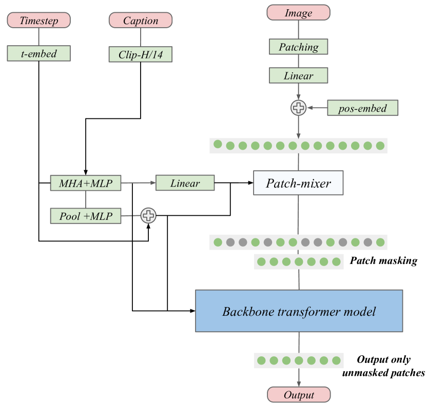
Improving backbone transformer architecture with mixture-of-experts (MoE) and layer-wise scaling. We also leverage innovations in transformer architecture design to boost the performance of our model under computational constraints. We use mixture-of-experts layers as they increase the parameters and expressive power of our model without significantly increasing the training cost (Shazeer et al., 2017; Fedus et al., 2022). We use a simplified MoE layer based on expert-choice routing (Zhou et al., 2022), where each expert determines the tokens routed to it, as it doesn’t require any additional auxiliary loss functions to balance the load across experts (Shazeer et al., 2017; Zoph et al., 2022). We also consider a layer-wise scaling approach, which has recently been shown to outperform canonical transformers in large-language models (Mehta et al., 2024). It linearly increases the width, i.e., hidden layer dimension in attention and feedforward layers, of transformer blocks. Thus, deeper layers in the network are assigned more parameters than earlier layers. We argue that since deeper layers in visual models tend to learn more complex features (Zeiler & Fergus, 2014), using higher parameters in deeper layers would lead to better performance. We provide background details on both techniques in Appendix B. We describe the overall architecture of our diffusion transformer in Figure 3.

Figure 3: Overall architecture of our diffusion transformer. We prepend the backbone transformer model with a lightweight patch-mixer that operates on all patches in the input image before they are masked. Following contemporary works (Betker et al., 2023; Esser et al., 2024), we process the caption embeddings using an attention layer before using them for conditioning. We use sinusoidal embeddings for timesteps. Our model only denoises unmasked patches, thus the diffusion loss (Eq. 3) is calculated only on these patches. We modify the backbone transformer using layer-wise scaling on individual layers and use mixture-of-expert layers in alternate transformer blocks.

3 Experimental Setup

We provide key details in our experimental setup below and additional details in Appendix A.

We use two variants of Diffusion Transformer (DiT) architecture from Peebles & Xie (2023): DiT-Tiny/2 and DiT-Xl/2, both comprising a patch size of $2$. When training sparse models, we replace every alternate transformer block with an 8-expert mixture-of-experts block. We train all models using the AdamW optimizer with cosine learning rate decay and high weight decay. We provide an exhaustive list of our training hyperparameters in Table 5 in Appendix A. We use a four-channel variational autoencoder (VAE) from the Stable-Diffusion-XL (Podell et al., 2024) model to extract image latents. We also consider the latest 16-channel VAEs for test their performance in large-scale micro-budget training (Esser et al., 2024). We use the EDM framework from Karras et al. (2022) as a unified training setup for all diffusion models. We refer to our diffusion trasnformer as MicroDiT. We use Fréchet inception distance (FID) (Heusel et al., 2017), both with the original Inception-v3 model (Szegedy et al., 2016) and a CLIP model (Radford et al., 2021), and CLIP score (Hessel et al., 2021) to measure the performance of the image generation models.

Choice of text encoder. To convert natural language captions to higher-dimensional feature embeddings, we use the text encoder from state-of-the-art CLIP models (Ilharco et al., 2021; Fang et al., 2023). We favor CLIP models over T5-xxl (Raffel et al., 2020; Saharia et al., 2022) for text encoding, despite the better performance of the latter on challenging tasks like text synthesis, as the latter incurs much higher computational and storage costs at scale, thus not suitable for micro-budget training (Table 6 in Appendix A). We consider the computation of text embeddings for captions and latent compression of images as a one-time cost that amortizes over multiple training runs of a diffusion model. Thus, we compute them offline and do not account for these costs in our estimation of training costs. We use a $30/hour cost estimate for an 8$\times$H100 GPU node (equivalent to $12/hour for an 8$\times$A100 GPU node) to measure the economical cost.

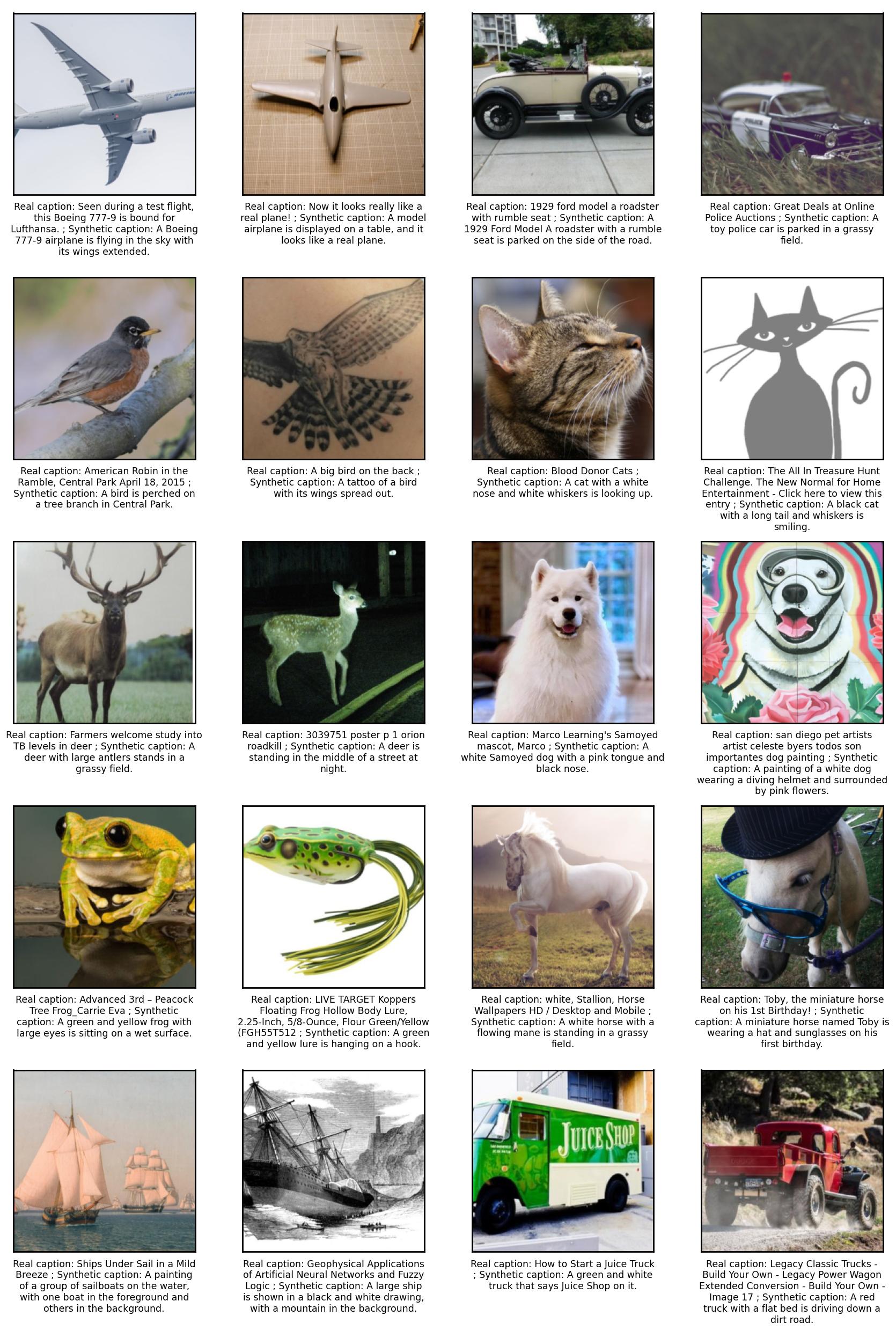
Training datasets. We use the following three real image datasets comprising $22M$ image-text pairs: Conceptual Captions (CC12M) (Changpinyo et al., 2021), Segment Anything (SA1B) (Kirillov et al., 2023), and TextCaps (Sidorov et al., 2020). As SA1B does not provide real captions, we use synthetic captions generated from an LLaVA model (Liu et al., 2023; Chen et al., 2023). We also add two synthetic image datasets comprising $15M$ image-text pairs in large-scale training: JourneyDB (Sun et al., 2024) and DiffusionDB (Wang et al., 2022). For small-scale ablations, we construct a text-to-image dataset, named cifar-captions, by subsampling images of ten CIFAR-10 classes from the larger COYO-700M (Byeon et al., 2022) dataset. Thus, cifar-captions serves as a drop-in replacement for any image-text dataset and simultaneously enables fast convergence due to being closed-domain. We provide additional details on construction of this dataset in Appendix A and samples images in Figure 28.

4 Evaluating Effectiveness of Deferred Masking

In this section, we validate the effectiveness of our deferred masking approach and investigate the impact of individual design choices on image generation performance. We use the DiT-Tiny/2 model and the cifar-captions dataset ($256\times 256$ image resolution) for all experiments in this section. We train each model for $60$K optimization steps, with the AdamW optimizer and exponential moving average with a $0.995$ smoothing coefficient enabled for the last $10$K steps.

4.1 Out-of-the-box performance: Making high masking ratios feasible with deferred masking

A key limitation of patch masking strategies is poor performance when a large fraction of patches are masked. For example, Zheng et al. (2024) observed large degradation in even MaskDiT performance beyond a 50% masking ratio. Before optimizing the performance of our approach with a rigorous ablation study, we evaluate its out-of-the-box performance with common training parameters for up to $87.5\%$ masking ratios. As a baseline, we train a network with no patch-mixer, i.e., naive masking (Figure 2c) for each masking ratio. For deferred masking, we use a four-transformer block patch-mixer that comprises less than $10$% of the parameters of the backbone transformer.

We use commonly used default hyperparameters to simulate the out-of-the-box performance for both our approach and the baseline. We train both models with the AdamW optimizer with an identical learning rate of $1.6\times 10^{-4}$, $0.01$ weight decay, and a cosine learning rate schedule. We set $(P_{\text{mean}},P_{\text{std}})$ to $(-1.2,1.2)$ following the original work (Karras et al., 2022). We provide our results in Figure 4. Our deferred masking approach achieves much better performance across all three performance metrics. Furthermore, the performance gaps widen with an increase in masking ratio. For example, with a 75% masking ratio, naive masking degrades the FID score to $16.5$ while our approach achieves $5.03$, much closer to the FID score of $3.79$ with no masking.

Figure 4: Out-of-the-box performance of deferred masking. Without any hyperparameter optimization, we compare the performance of our deferred masking with a naive masking strategy. We find that deferred masking, i.e., using a patch-mixer before naive masking, tremendously improves image generation performance, particularly at high masking ratios.

4.2 Ablation study of our training pipeline

We ablate design choices across masking, patch mixer, and training hyperparameters. We summarize the techniques that improved out-of-the-box performance in Table 5(a). We provide supplementary results and discussion of the ablation study in Appendix C.

Comparison with training hyperparameters of LLMs. Since the diffusion architectures are very similar to transformers used in large language models (LLMs), we compare the hyperparameter choices across the two tasks. Similar to common LLM training setups (Touvron et al., 2023; Jiang et al., 2023; Chowdhery et al., 2022), we find that SwiGLU activation (Shazeer, 2020) in the feedforward layer outperforms the GELU (Hendrycks & Gimpel, 2016) activation function. Similarly, higher weight decay leads to better image generation performance. However, we observe better performance when using a higher running average coefficient for the AdamW second moment ($\beta_{2}$), in contrast to large-scale LLMs where $\beta_{2}\approx 0.95$ is preferred. As we use a small number of training steps, we find that increasing the learning rate to the maximum possible value until training instabilities also significantly improves image generation performance.

Design choices in masking and patch-mixer. We observe a consistent improvement in performance with a larger patch mixer. However, despite the better performance of larger patch-mixers, we choose to use a small patch mixer to lower the computational budget spent by the patch mixer in processing the unmasked input. We also update the noise distribution $(P_{\text{mean}},P_{\text{std}})$ to $(-0.6,1.2)$ as it improves the alignment between captions and generated images. By default, we mask each patch at random. We ablate the masking strategy to retain more continuous regions of patches using block masking (Figure 5(b)). However, we find that increasing the block size leads to a degradation in the performance of our approach, thus we retain the original strategy of masking each patch at random.

	FID ($\downarrow$)	Clip-FID ($\downarrow$)	Clip-score ($\uparrow$)
Out-of-box	$8.82$	$5.03$	$26.72$
Higher weight decay	$8.38$	$4.90$	$27.00$
Sigma distribution	$8.49$	$4.93$	$27.47$
Larger patch-mixer	$7.40$	$4.57$	$27.79$
Higher learning rate	$7.09$	$4.10$	$28.24$

(a) Summarizing the factors that led to improved performance during our ablation study. We conduct this ablation study at $75\%$ masking ratio. Detailed results provided in Table 11 in Appendix C.

(b) Is block masking of patches more effective? We retain a continuous region of image patches using block masking to test its impact on image generation performance. In this figure, we illustrate the masks for $75\%$ masking ratio with varying block sizes. By default, we mask each patch randomly, i.e., block size ($b$) = 1.

4.3 Validating improvements in diffusion transformer architecture

We measure the effectiveness of the two modifications in transformer architecture in improving image generation performance.

Table 1: Layer-wise scaling of transformer architecture is a better fit for masked training in diffusion transformers. We validate its effectiveness in the canonical naive masking with $75\%$ masking ratio.

Arch	FID ($\downarrow$)	Clip-FID ($\downarrow$)	Clip-score ($\uparrow$)
Constant width	$19.6$	$9.9$	$26.7$
Layer-wise scaling	$\mathbf{15.9}$	$\mathbf{7.4}$	$\mathbf{27.1}$

Layer-wise scaling. We investigate the impact of this design choice in a standalone experiment where we train two variants of a DiT-Tiny architecture, one with a constant width transformer and the other with layer-wise scaling of each transformer block. We use naive masking for both methods. We select the width of the constant-width transformer such that its computational footprint is identical to layer-wise scaling. We train both models for an identical number of training steps and wall-clock time. We find that the layer-wise scaling approach outperforms the baseline constant width approach across all three performance metrics (Table 1), demonstrating a better fit of the layer-wise scaling approach in masked training of diffusion transformers.

Mixture-of-experts layers. We train a DiT-Tiny/2 transformer with expert-choice routing based mixture-of-experts (MoE) layers in each alternate transformer block. On the small-scale setup, it achieves similar performance to baseline model trained without MoE blocks. While it slightly improves Clip-score from $28.11$ to $28.66$, it degrades FID score from $6.92$ to $6.98$. We hypothesize that the lack of improvement is due to the small number of training steps ($60$K) as using multiple experts effectively reduces the number of samples observed by each router. In top-2 routing for 8-experts, each expert is trained effectively for one fourth number of epochs over the dataset. We observe a significantly improvement in performance with MoE blocks when training on scale for longer training schedules (Section 6.2).

Figure 6: Comparing performance of patch masking strategies. Using a lightweight patch-mixer before patch masking in our deferred masking approach significantly improves image generation performance over baseline masking strategies. Our approach incurs near identical training cost as the MaskDiT (Zheng et al., 2024) baseline. However, both approaches incur slightly higher cost than naive masking due the use of an additional lightweight transformer along with the backbone diffusion transformer.

5 Comparing the Effectiveness of Deferred Masking with Baselines

In this section, we provide a concrete comparison with multiple baselines. First, we compare with techniques aimed at reducing computational cost by reducing the transformer patch sequence size. Next, we consider reducing network size, i.e., downscaling, while keeping the patch sequence intact. Under isoflops budget, i.e., identical wall-clock training time and FLOPs, we show that our approach achieves better performance than model downscaling.

Comparing different masking strategies. We first compare our approach with the strategy of using larger patches. We increase the patch size from two to four, equivalent to 75% patch masking. However, it underperforms compared to deferred masking and only achieves $9.38$, $6.31$, and $26.70$ FID, Clip-FID, and Clip-score, respectively. In contrast, deferred masking achieves $7.09$, $4.10$, and $28.24$ FID, Clip-FID, and Clip-score, respectively. Next, we compare all three masking strategies (Figure 2). We train each model for $60$K steps and report total training flops for each approach to indicate its computational cost. We find that naive masking significantly degrades model performance, and using additional proxy loss functions (Zheng et al., 2024) only marginally improves performance. We find that simply deferring the masking and using a small transformer as a patch-mixer significantly bridges the gap between masked and unmasked training of diffusion transformers.

IsoFLOPs study - Why bother using masking instead of smaller transformers? Using patch masking is a complementary approach to downscaling transformer size to reduce computation cost in training. We compare the two approaches in Table 7(a). At each masking ratio, we reduce the size of the unmasked network to match FLOPs and total wall-clock training time of masked training. We train both networks for $60$K training steps. Until a masking ratio of 75%, we find that deferred masking outperforms network down-scaling across at least two out of three metrics. However, at extremely high masking ratios, deferred masking tends to achieve lower performance. This is likely because the information loss from masking is too high at these ratios. For example, for $32\times 32$ resolution latent and a patch size of two, only $32$ patches are retained (out of $256$ patches) at an 87.5% masking ratio.

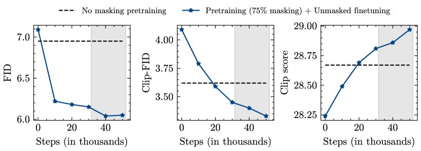
Deferred masking as pretraining $+$ unmasked finetuning. We show deferred masking also acts as a strong pretraining objective and using it with an unmasked finetuning schedule achieves better performance than training an unmasked network under an identical computational budget. We first train a network without any masking and another identical network with 75% deferred masking. We finetune the latter with no masking and measure performance as we increase the number of finetuning steps. We mark the isoflops threshold when the combined cost of masked pretraining and unmasked finetuning is identical to the model trained with no masking. We find that at the isoflops threshold, the finetuned model achieves superior performance across all three performance metrics. The performance of the model also continues to improve with unmasked finetuning steps beyond the isoflops threshold.

Masking ratio	Masking ratio	FID	Clip-FID	Clip-score
Downscaled network	-	$\mathbf{6.60}$	$3.85$	$28.49$
Deferred masking	$0.5$	$6.74$	$\mathbf{3.45}$	$\mathbf{28.86}$
Downscaled network	-	$7.09$	$4.56$	$27.68$
Deferred masking	$0.75$	$\mathbf{6.96}$	$\mathbf{4.17}$	$\mathbf{28.16}$
Downscaled network	-	$\mathbf{7.52}$	$\mathbf{5.03}$	$26.98$
Deferred masking	$0.875$	$8.35$	$5.26$	$\mathbf{27.00}$

(a) IsoFLOPs training. Under identical training setup and wall-clock time, we compare the effectiveness of model downscaling and our deferred masking approaches. We find that except at extremely high masking ratios, deferred masking achieves better performance across at least two performance metrics. Based on this finding, we do not use a masking ratio higher than 75% in our models.

(b) Unmasked finetuning. After pretraining with 75% deferred masking, we increase the number of unmasked finetuning steps and compare its performance with another model trained completely without masking. The shaded region represents steps after the isoflops threshold, where deferred masking pretraining and finetuning have higher computation cost. At the isoflops threshold, the finetuned model achieves better performance than training the diffusion model without any masking.

Figure 7: Deferred masking vs. model downscaling to reduce training cost. Both patch masking and model downscaling, i.e., reducing the size of the model, reduce the computational cost in training and can be complementary to each other. However, it is natural to ask how the two paradigms compare to each other in training diffusion transformers. In figure (a), we show that reducing the model size, thus reducing the total computational budget of training, achieves inferior performance compared to our approach at masking ratios under 75%. Using a patch-mixer in deferred masking effectively enables our model to simultaneously observe all patches in input images while reducing the effective number of patches processed per image. This result encourages using a larger model with masking rather than training a smaller model with no masking for equivalent computational cost. In figure (b), we further highlight the advantage of using deferred masking with finetuning over training a model with no masking for a given computational budget.

Table 2: Computational cost of the two-stage training of our large-scale model. Our total computational cost is $3.45\times 10^{20}$ FLOPs, amounting to a total cost of $1,890 and $2.6$ training days on an 8$\times$H100 GPU machine.

Resolution	Masking ratio	Training steps	Total FLOPs	$8\times$A100 days	$8\times$H100 days	Cost ($)
$256\times 256$	$0.75$	$250000$	$1.47\times 10^{20}$	$2.77$	$1.11$	$800$
	$0.00$	$30000$	$4.53\times 10^{19}$	$0.94$	$0.38$	$271$
$512\times 512$	$0.75$	$50000$	$1.18\times 10^{20}$	$2.18$	$0.88$	$630$
	$0.00$	$5000$	$3.48\times 10^{19}$	$0.65$	$0.26$	$189$

6 Micro-budget Training of Large-scale Models

In this section, we validate the effectiveness of our approach in training open-world text-to-image generative models on a micro-budget. Moving beyond the small-scale cifar-captions dataset, we train the large-scale model on a mixture of real and synthetic image datasets comprising $37$M images. We demonstrate the high-quality image generation capability of our model and compare its performance with previous works across multiple quantitative metrics.

Training process. We train a DiT-Xl/2 transformer with eight experts in alternate transformer blocks. We provide details on training hyperparameters in Table 5 in the Appendix A. We conduct the training in follwoing two phases. We refer to any diffusion transformer trained using our micro-budget training as MicroDiT.

• Phase-1: In this phase, we pretrain the model on $256\times 256$ resolution images. We train for $250$K optimization steps with $75\%$ patch masking and finetune for another $30$K steps without any patch masking.

• Phase-2: In this phase, we finetune the Phase-1 model on $512\times 512$ resolution images. We first finetune the model for $50$K steps with $75\%$ patch masking followed by another $5$K optimization steps with no patch masking.

Computational cost. We provide a breakdown of computational cost, including both training FLOPs and economical cost, across each training phase in Table 2. Our Phase-1 and Phase-2 training consumes $56\%$ and $44\%$ of the total computational cost, respectively. The total wall-clock training time of our model is $2.6$ days on an $8\times$H100 GPU cluster, equivalent to $6.6$ days on an $8\times$A100 GPU cluster.

(a) DrawBench

(b) PartiPrompts

Figure 8: Assesssing image quality with GPT-4o. We supply the following prompt to the GPT-4o model: Given the prompt ‘{prompt}’, which image do you prefer, Image A or Image B, considering factors like image details, quality, realism, and aesthetics? Respond with ’A’ or ’B’ or ’none’ if neither is preferred. For each comparison, we also shuffle the order of images to remove any ordering bias. We evaluate the performance on two prompt databases: DrawBench (Saharia et al., 2022) and PartiPrompts (Yu et al., 2022). The y-axis in the bar plots indicates the percentage of comparisons in which image from a model is preferred. We breakdown the comparison across individual image category in each prompt database.

Figure 9: Synthesized images from a model trained only on real data (on left) and combined real and synthetic data (on right). Real data includes SA1B, CC12M, and TextCaps datasets while synthetic data includes JourneyDB and DiffusionDB datasets.

6.1 Benefit of additional synthetic data in training

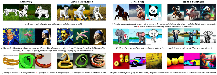
Instead of training only on real images, we expand the training data to include 40% additional synthetic images. We compare the performance of two MicroDiT models trained on only real images and combined real and synthetic images, respectively, using identical training processes.

Under canonical performance metrics, both models apparently achieve similar performance. For example, the model trained on real-only data achieved an FID score of 12.72 and a CLIP score of 26.67, while the model trained on both real and synthetic data achieved an FID score of 12.66 and a CLIP score of 28.14. Even on GenEval (Ghosh et al., 2024), a benchmark that evaluates the ability to generate multiple objects and modelling object dynamics in images, both models achieved an identical score of 0.46. These results seemingly suggest that incorporating a large amount of synthetic samples didn’t yield any meaningful improvement in image generation capabilities.

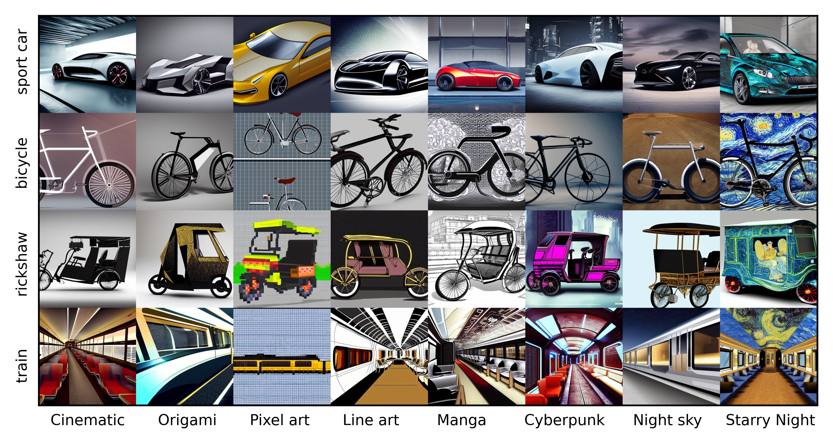
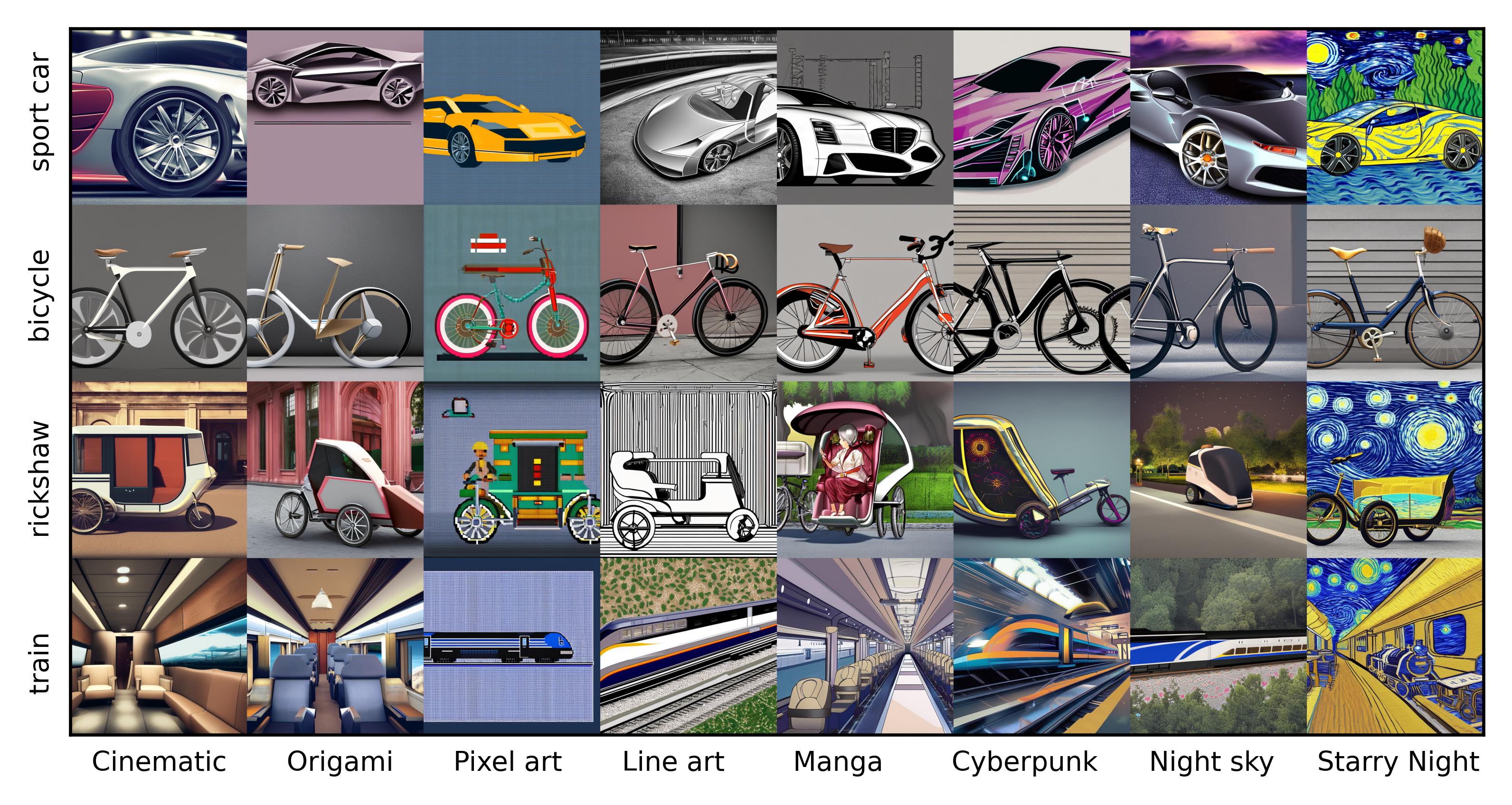
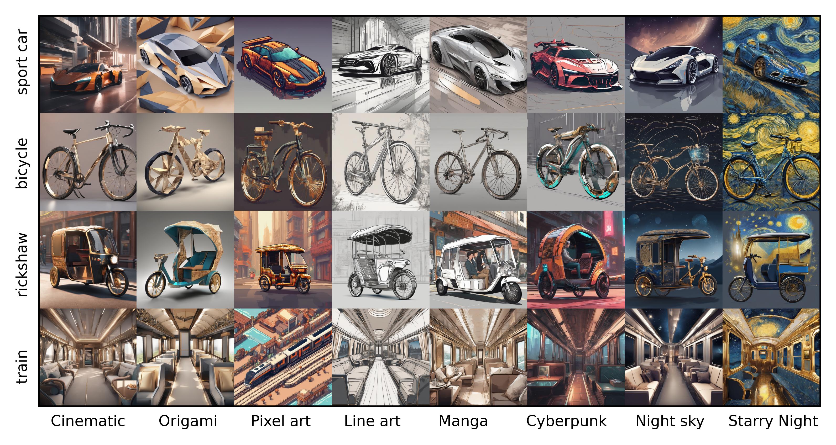
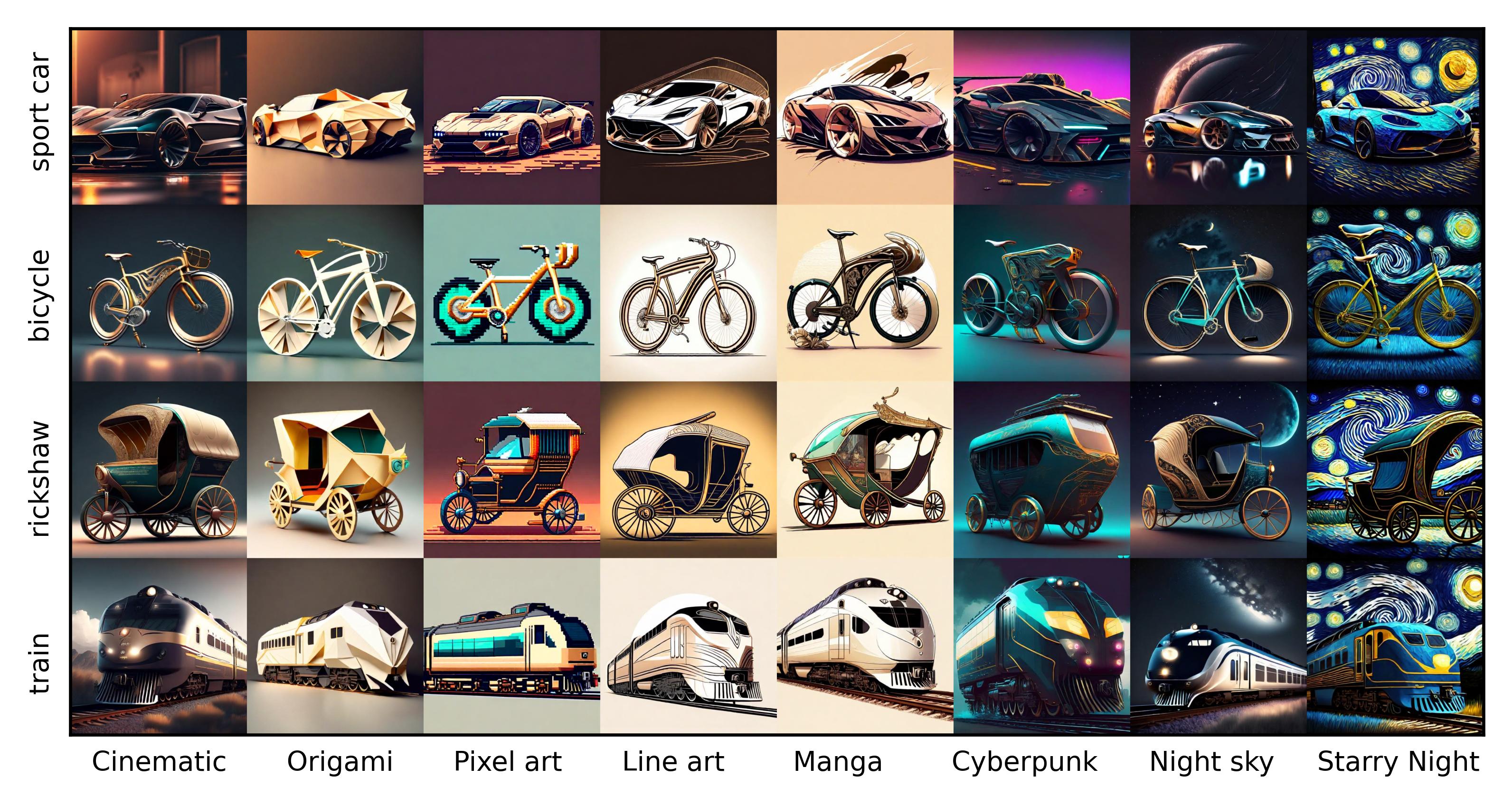
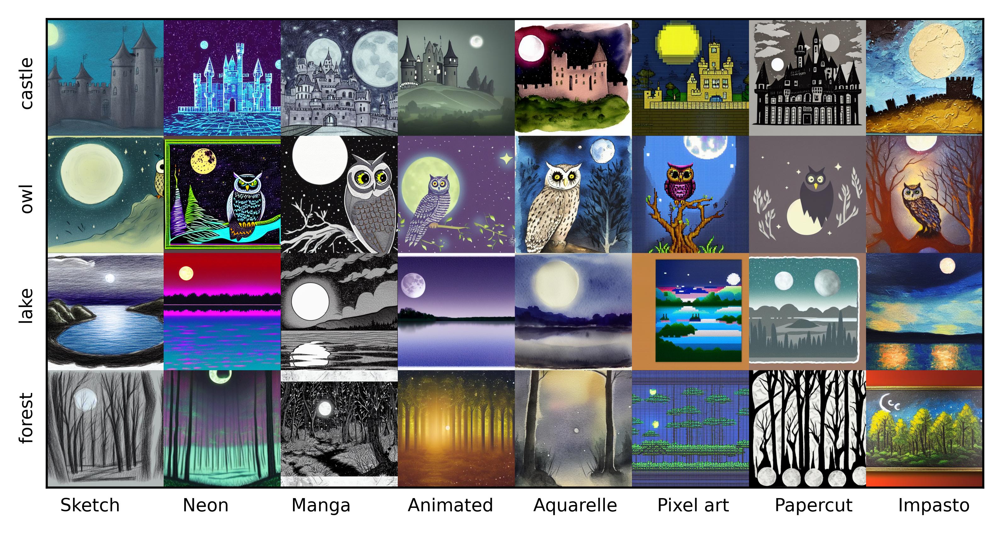
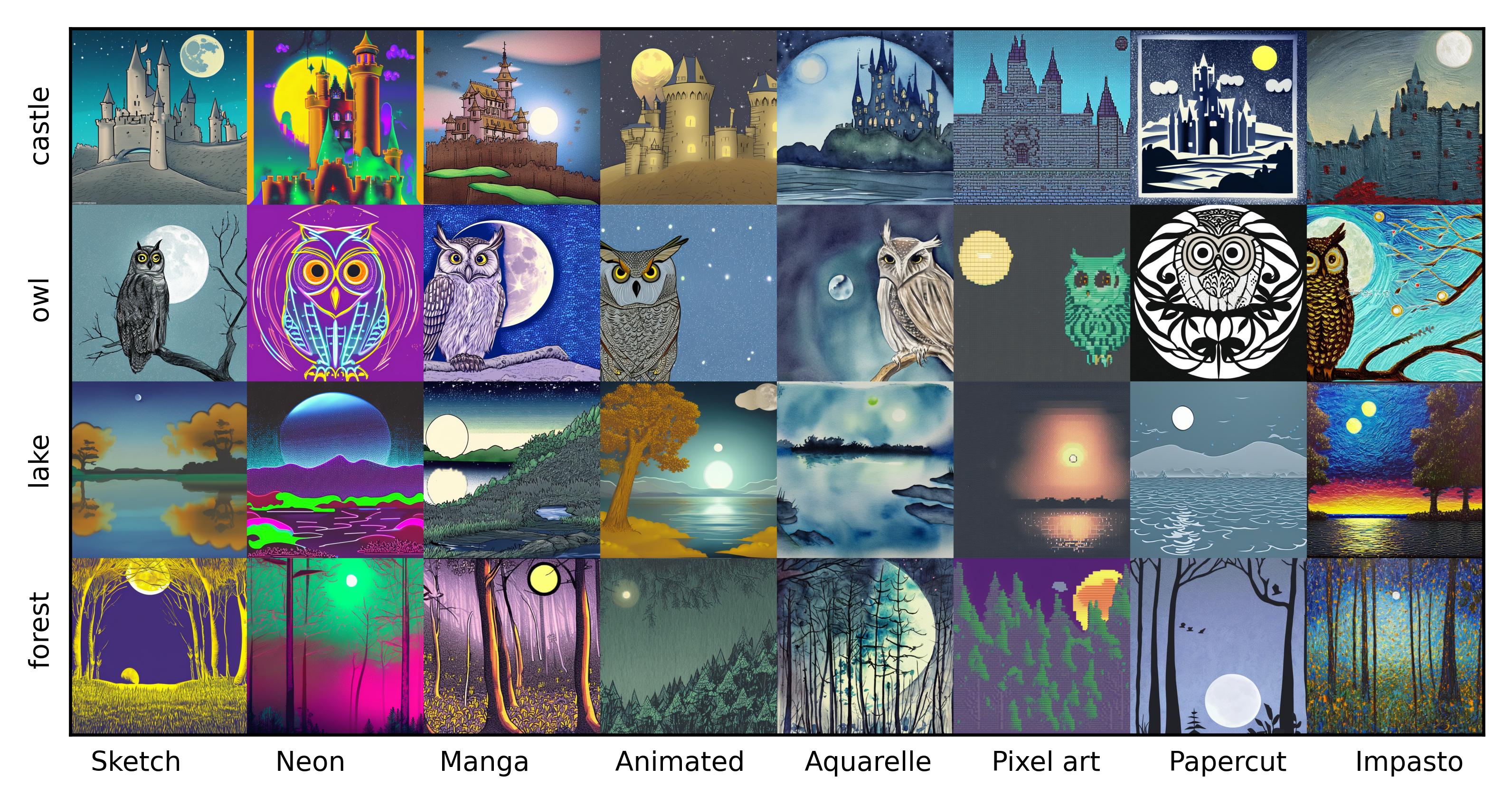
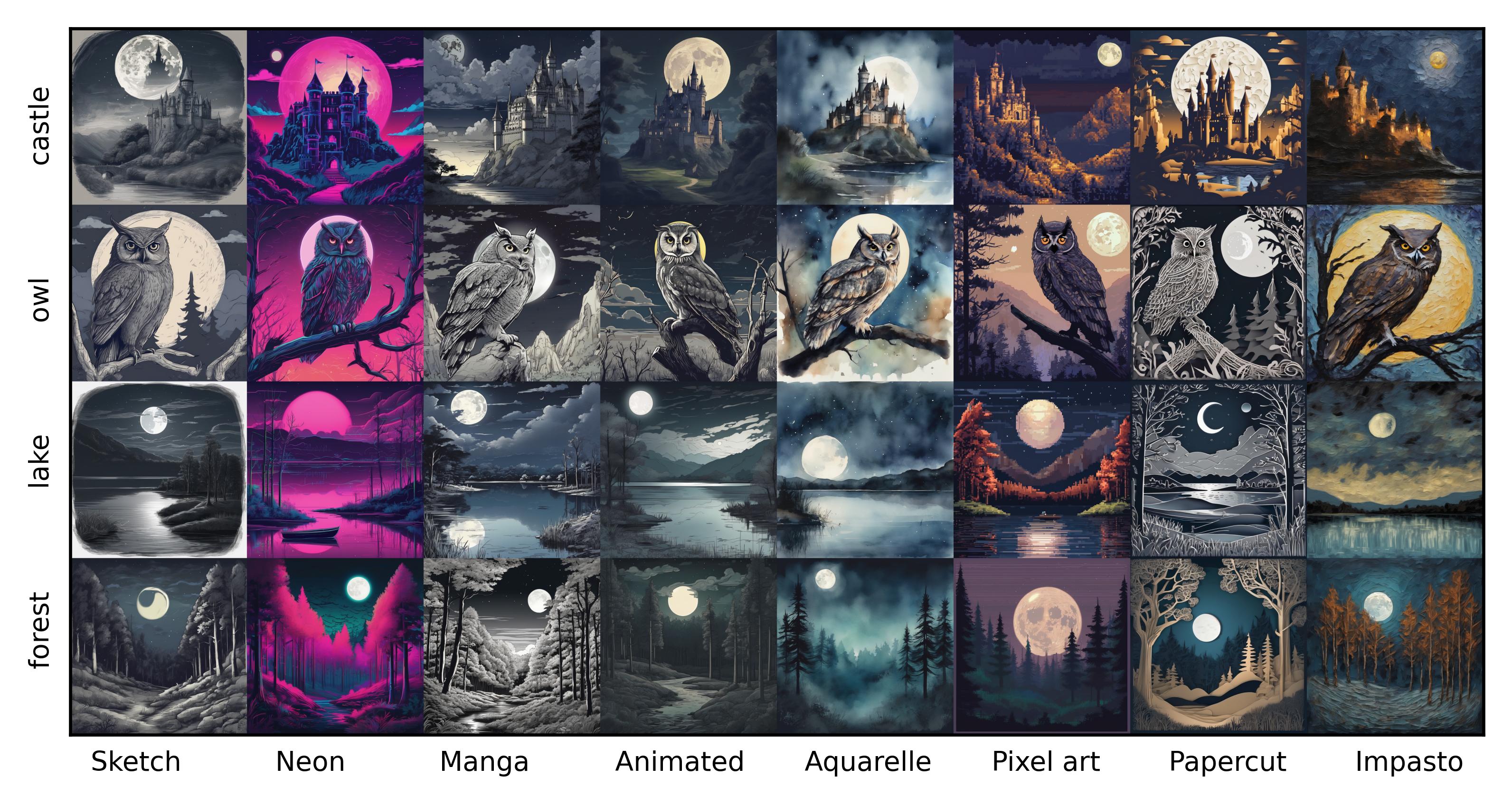
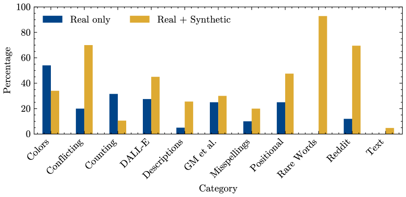
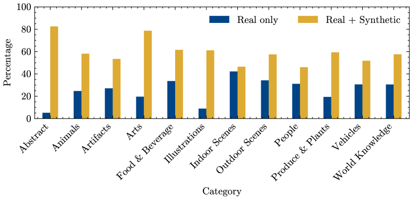
However, we argue that this observation is heavily influenced by the limitations of our existing evaluation metrics. In a qualitative evaluation, we found that the model trained on the combined dataset achieved much better image quality (Figure 9). The real data model often fails to adhere to the prompt, frequently hallucinating key details and often failing to synthesize the correct object. Metrics, such as FID, fail to capture this difference because they predominantly measure distribution similarity (Pernias et al., 2024). Thus, we focus on using human visual preference as an evaluation metric. To automate the process, we use GPT-4o (OpenAI, 2024), a state-of-the-art multimodal model, as a proxy for human preference. We supply the following prompt to the model: Given the prompt ‘{prompt}’, which image do you prefer, Image A or Image B, considering factors like image details, quality, realism, and aesthetics? Respond with ’A’ or ’B’ or ’none’ if neither is preferred. For each comparison, we also shuffle the order of images to remove any ordering bias. We generate samples using DrawBench (Saharia et al., 2022) and PartiPrompts (P2) (Yu et al., 2022), two commonly used prompt databases (Figure 9). On the P2 dataset, images from the combined data model are preferred in 63% of comparisons while images from the real data model are only preferred 21% of the time (16% of comparisons resulted in no preference). For the DrawBench dataset, the combined data model is preferred in 40% of comparisons while the real data model is only preferred in 21% of comparisons. Overall, using a human preference-centric metric clearly demonstrates the benefit of additional synthetic data in improving overall image quality.

(a) Measuring fidelity and prompt alignment of generated images on COCO dataset.

Channels	FID-30K ($\downarrow$)	Clip-FID-30K ($\downarrow$)	Clip-score ($\uparrow$)
$4$	$\mathbf{12.65}$	$\mathbf{5.96}$	$\mathbf{28.14}$
$16$	$13.04$	$6.84$	$25.63$

(b) Measuring performance on the GenEval benchmark.

		Objects
Channels	Overall	Single	Two	Counting	Colors	Position	Color attribution
4	$\mathbf{0.46}$	$\mathbf{0.97}$	$\mathbf{0.47}$	$\mathbf{0.33}$	$\mathbf{0.78}$	$\mathbf{0.09}$	$\mathbf{0.20}$
16	0.40	0.96	0.36	0.27	0.72	0.07	0.09

Figure 10: We ablate the dimension of latent space by training our MicroDiT models in four and sixteen channel latent space, respectively. Even though training in higher dimensional latent space is being adopted across large-scale models (Esser et al., 2024; Dai et al., 2023) we find that it underperforms when training on a micro-budget.

Model	Params ($\downarrow$)	Sampling steps ($\downarrow$)	Open-source	Training images($\downarrow$)	8$\times$A100 GPU days ($\downarrow$)	FID-30K ($\downarrow$)
CogView2 (Ding et al., 2022)	$6.00$B	$-$	$-$	$-$	$-$	$24.0$
Dall-E (Ramesh et al., 2021)	$12.0$B	$256$	$-$	$-$	$-$	$17.89$
Glide (Nichol et al., 2021)	$3.50$B	$250$	$-$	$-$	$-$	$12.24$
Parti-750M (Yu et al., 2022)	$0.75$B	$1024$	$-$	$3690$M	$-$	$10.71$
Dall-E.2 (Ramesh et al., 2022)	$6.50$B	$-$	$-$	$650$M	$5208.3$	$10.39$
Make-a-Scene (Gafni et al., 2022)	$4.00$B	$1024$	$-$	$-$	$-$	$11.84$
GigaGAN (Kang et al., 2023)	$1.01$B	$1$	$-$	$980$M	$597.8$	$9.09$
ImageN (Saharia et al., 2022)	$3.00$B	$-$	$-$	$860$M	$891.5$	$7.27$
Parti-20B (Yu et al., 2022)	$20.0$B	$1024$	$-$	$3690$M	$-$	$7.23$
eDiff-I (Balaji et al., 2022)	$9.10$B	$25$	$-$	$11470$M	$-$	$6.95$
Stable-Diffusion-2.1a (Rombach et al., 2022)	$0.86$B	$50$	$\checkmark$	$3900$M	$1041.6$	$9.12$
Stable-Diffusion-1.5 (Rombach et al., 2022)	$0.86$B	$50$	$\checkmark$	$4800$M	$781.2$	$11.18$
Würstchen (Pernias et al., 2024)	$0.99$B	$60$	$\checkmark$	$1420$M	$128.1$	$23.60$
PixArt-$\alpha$ (Chen et al., 2023)	$0.61$B	$20$	$\checkmark$	$25$Mb	$94.1$c	$7.32$
MicroDiT (our work)	$1.16$B	$30$	$\checkmark$	$37$M	$\mathbf{6.6}$	$12.66$

• As the FID scores for the stable diffusion models are not officially reported (Rombach et al., 2022), we calculate them using the official release of each model. We achieve slightly better FID scores compared to the scores reported in Würstchen (Pernias et al., 2024). We use our FID scores to represent the best performance of these models.

• Includes 10M proprietary high-quality images.

• PixArt-$\alpha$ training takes 85 days on an 8$\times$A100 machine when only training till $512\times 512$ resolution.

Table 3: Zero-shot FID on COCO2014 validation split (Lin et al., 2014). We report total training time in terms of number of days required to train the model on a machine with eight A100 GPUs. We observe a $2.5\times$ reduction in training time when using H100 GPUs. Our micro-budget training takes $14.2\times$ less training time than state-of-the-art low-cost training approach while simultaneously achieving competitive FID compared to some open-source models.

Table 4: Comparing performance on compositional image generation using GenEval (Ghosh et al., 2024) benchmark. Table adopted from Esser et al. (2024). Higher performance is better.

			Objects
Model	Open-source	Overall	Single	Two	Counting	Colors	Position	Color attribution
DaLL-E.2 (Ramesh et al., 2022)	$-$	0.52	0.94	0.66	0.49	0.77	0.10	0.19
DaLL-E.3 (Betker et al., 2023)	$-$	0.67	0.96	0.87	0.47	0.83	0.43	0.45
minDALL-E (Kim et al., 2021)	$\checkmark$	0.23	0.73	0.11	0.12	0.37	0.02	0.01
Stable-Diffusion-1.5 (Rombach et al., 2022)	$\checkmark$	0.43	0.97	0.38	0.35	0.76	0.04	0.06
PixArt-$\alpha$ (Chen et al., 2023)	$\checkmark$	0.48	0.98	0.50	0.44	0.80	0.08	0.07
Stable-Diffusion-2.1 (Rombach et al., 2022)	$\checkmark$	0.50	0.98	0.51	0.44	0.85	0.07	0.17
Stable-Diffusion-XL (Podell et al., 2024)	$\checkmark$	0.55	0.98	0.74	0.39	0.85	0.15	0.23
Stable-Diffusion-XL-Turbo (Sauer et al., 2023)	$\checkmark$	0.55	1.00	0.72	0.49	0.80	0.10	0.18
IF-XL	$\checkmark$	0.61	0.97	0.74	0.66	0.81	0.13	0.35
Stable-Diffusion-3 (Esser et al., 2024)	$\checkmark$	0.68	0.98	0.84	0.66	0.74	0.40	0.43
MicroDiT (our work)	$\checkmark$	0.46	0.97	0.47	0.33	0.78	0.09	0.20

6.2 Ablating design choices on scale

We first examine the effect of using a higher dimensional latent space in micro-budget training. We replace the default four-channel autoencoder with one that has sixteen channels, resulting in a $4\times$ higher dimensional latent space. Recent large-scale models have adopted high dimensional latent space as it provides significant improvements in image generation abilities (Dai et al., 2023; Esser et al., 2024). Note that the autoencoder with higher channels itself has superior image reconstruction capabilities, which further contributes to overall success. Intriguingly, we find that using a higher dimensional latent space in micro-budget training hurts performance. For two MicroDiT models trained with identical computational budgets and training hyperparameters, we find that the model trained in four-channel latent space achieves better FID, Clip-score, and GenEval scores (Table 10). We hypothesize that even though an increase in latent dimensionality allows better modeling of data distribution, it also simultaneously increases the training budget required to train higher quality models. We also ablate the choice of mixture-of-experts (MoE) layers by training another MicroDiT model without them under an identical training setup. We find that using MoE layers improves zero-shot FID-30K from 13.7 to 12.7 on the COCO dataset. Due to the better performance of the sparse transformers with MoE layers, we use MoE layers by default in large-scale training.

6.3 Comparison with previous works

Comparing zero-shot image generation on COCO dataset (Table 3). We follow the evaluation methodology in previous work (Saharia et al., 2022; Yu et al., 2022; Balaji et al., 2022) and sample 30K random images and corresponding captions from the COCO 2014 validation set. We generate 30K synthetic images using the captions and measure the distribution similarity between real and synthetic samples using FID (referred to as FID-30K in Table 3). Our model achieves a competitive 12.66 FID-30K, while trained with $14\times$ lower computational cost than the state-of-the-art low-cost training method and without any proprietary or humongous dataset to boost performance. Our approach also outperforms Würstchen (Pernias et al., 2024), a recent low-cost training approach for diffusion models, while requiring $19\times$ lower computational cost.

Fine-grained image generation comparison (Table 4). We use the GenEval (Ghosh et al., 2024) framework to evaluate the compositional image generation properties, such as object positions, co-occurrence, count, and color. Similar to most other models, our model achieves near perfect accuracy on single-object generation. Across other tasks, our model performs similar to early Stable-Diffusion variants, notably outperforming Stable-Diffusion-1.5. On the color attribution task, our model also outperforms Stable-Diffusion-XL-turbo and PixArt-$\alpha$ models.

7 Related work

The landscape of diffusion models (Sohl-Dickstein et al., 2015; Ho et al., 2020; Song et al., 2020a; b) has rapidly evolved in the last few years, with modern models trained on web-scale datasets (Betker et al., 2023; Esser et al., 2024; Rombach et al., 2022; Saharia et al., 2022). In contrast to training in pixel space (Saharia et al., 2022; Nichol et al., 2021), the majority of large-scale diffusion models are trained in a compressed latent space, thus referred to as latent diffusion models (Rombach et al., 2022). Similar to auto-regressive models, transformer architectures (Vaswani et al., 2017) have also been recently adopted for diffusion-based image synthesis. While earlier models commonly adopted a fully convolutional or hybrid UNet network architecture (Dhariwal & Nichol, 2021; Nichol et al., 2021; Rombach et al., 2022; Saharia et al., 2022), recent works have demonstrated that diffusion transformers (Peebles & Xie, 2023) achieve better performance (Esser et al., 2024; Chen et al., 2023; Betker et al., 2023). Thus, we also use diffusion transformers for modeling latent diffusion models.

Since the image captions in web-scale datasets are often noisy and of poor quality (Byeon et al., 2022; Schuhmann et al., 2022), recent works have started to recaption them using vision-language models (Liu et al., 2023; Wang et al., 2023; Li et al., 2024). Using synthetic captions leads to significant improvements in the diffusion models’ image generation capabilities (Betker et al., 2023; Esser et al., 2024; Gokaslan et al., 2024; Chen et al., 2023). While text-to-image generation models are the most common application of diffusion models, they can also support a wide range of other conditioning mechanisms, such as segmentation maps, sketches, or even audio descriptions (Zhang et al., 2023; Yariv et al., 2023). Sampling from diffusion models is also an active area of research, with multiple novel solvers for ODE/SDE sampling formulations to reduce the number of iterations required in sampling without degrading performance (Song et al., 2020a; Jolicoeur-Martineau et al., 2021; Liu et al., 2022; Karras et al., 2022). Furthermore, the latest approaches enable single-step sampling from diffusion models using distillation-based training strategies (Song et al., 2023; Sauer et al., 2023). The sampling process in diffusion models also employs an additional guidance signal to improve prompt alignment, either based on an external classifier (Dhariwal & Nichol, 2021; Nichol et al., 2021; Sehwag et al., 2022) or self-guidance (Ho & Salimans, 2022; Karras et al., 2024). The latter classifier-free guidance approach is widely adopted in large-scale diffusion models and has been further extended to large-language models (Zhao et al., 2024; Sanchez et al., 2023).

Since the training cost of early large-scale diffusion models was noticeably high (Rombach et al., 2022; Ramesh et al., 2022), multiple previous works focused on bringing down this cost. Gokaslan et al. (2024) showed that using common tricks from efficient deep learning can bring the cost of stable-diffusion-2 models under $50K. Chen et al. (2023) also reduced this cost by training a diffusion transformer model on a mixture of openly accessible and proprietary image datasets. Cascaded training of diffusion models is also used by some previous works (Saharia et al., 2022; Pernias et al., 2024; Guo et al., 2024), where multiple diffusion models are employed to sequentially upsample the low-resolution generations from the base diffusion model. A key limitation of cascaded training is the strong influence of the low-resolution base model on overall image fidelity and prompt alignment. Most recently, Pernias et al. (2024) adopted the cascaded training approach (Würstchen) while training the base model in a $42\times$ compressed latent space. Though Würstchen achieves low training cost due to extreme image compression, it also achieves significantly lower image generation performance on the FID evaluation metric. Alternatively, patch masking has been recently adopted as a means to reduce the computational cost of training diffusion transformers (Zheng et al., 2024; Gao et al., 2023), taking inspiration from the success of patch masking in contrastive models (He et al., 2022). Patch masking is straightforward to implement in transformers, and the diffusion transformer successfully generalizes to unmasked images in inference, even when patches for each image were masked randomly during training.

8 Discussion and Future Work

As the overarching objective of our work is to reduce the overhead of training large-scale diffusion models, we not only aim to reduce the training cost but also align design choices in the training setup with this objective. For example, we deliberately choose datasets that are openly accessible and show that using only these datasets suffices to generate high-quality samples, thus omitting the need for proprietary or enormous datasets. We also favor CLIP-based text embeddings which, although underperforming compared to T5 model embeddings (especially in text generation), are much faster to compute and require six times less disk storage.

While we observe competitive image generation performance with micro-budget training, it inherits the limitations of existing text-to-image generative models, especially in text rendering. It is surprising that the model learns to successfully adhere to complex prompts demonstrating strong generalization to novel concepts while simultaneously failing to render even simple words, despite the presence of a dedicated optical character recognition dataset in training. Similar to a majority of other open-source models, our model struggles with controlling object positions, count, and color attribution, as benchmarked on the GenEval dataset.

We believe that the lower overhead of large-scale training of diffusion generative models can dramatically enhance our understanding of training dynamics and accelerate research progress in alleviating the shortcomings of these models. It can enable a host of explorations on scale, in directions such as understanding end-to-end training dynamics (Agarwal et al., 2022; Choromanska et al., 2015; Jiang et al., 2020), measuring the impact of dataset choice on performance (Xie et al., 2024), data attribution for generated samples (Zheng et al., 2023; Dai & Gifford, 2023; Park et al., 2023; Koh & Liang, 2017), and adversarial interventions in the training pipeline (Chou et al., 2023; Shafahi et al., 2018). Future work can also focus on alleviating current limitations of micro-budget training, such as poor rendering of text and limitations in capturing intricate relationships between objects in detailed scenes. While we focus mainly on algorithmic efficiency and dataset choices, the training cost can be significantly reduced by further optimizing the software stack, e.g., by adopting native 8-bit precision training (Mellempudi et al., 2019), using dedicated attention kernels for H100 GPUs (Shah et al., 2024), and optimizing data loading speed.

9 Conclusion

In this work, we focus on patch masking strategies to reduce the computational cost of training diffusion transformers. We propose a deferred masking strategy to alleviate the shortcomings of existing masking approaches and demonstrate that it provides significant improvements in performance across all masking ratios. With a deferred masking ratio of 75%, we conduct large-scale training on commonly used real image datasets, combined with additional synthetic images. Despite being trained at an order of magnitude lower cost than the current state-of-the-art, our model achieves competitive zero-shot image generation performance. We hope that our low-cost training mechanism will empower more researchers to participate in the training and development of large-scale diffusion models.

10 Acknowledgements

We would like to thank Peter Stone, Felancarlo Garcia, Yihao Zhan, and Naohiro Adachi for their valuable feedback and support during the project. We also thank Weiming Zhuang, Chen Chen, Zhizhong Li, Sina Sajadmanesh, Jiabo Huang, Nidham Gazagnadou, and Vivek Sharma for their constructive feedback throughout the progress of this project.

Appendix A Additional details on experimental setup

We use DiT-Tiny/2 and DiT-Xl/2 diffusion transformer architectures for small and large scale training setups, respectively. We use four and six transformer blocks in the patch-mixer for the DiT-Tiny/2 and DiT-Xl/2 architectures, respectively. The patch-mixer comprises approximately 13% of the parameters in the backbone diffusion transformer. We use half-precision layernorm normalization and SwiGLU activation in the feedforward layers for all transformers. Initially, half-precision layernorm leads to training instabilities after $100$K steps of training. Thus, we further apply layer normalization to query and key embeddings in the attention layers (Dehghani et al., 2023), which stabilizes the training. We reduce the learning rate for expert layers by half as each expert now processes a fraction of all patches. We provide an exhaustive list of our training hyperparameters in Table 5. We use the default configuration ($\sigma_{\text{max}}=80,\sigma_{\text{min}}=0.002,S_{\text{max}}=\infty,S_{\text{noise}}=1,S_{\text{min}}=0,S_{\text{churn}}=0$), except that we increase $\sigma_{data}$ to match the standard deviation of our image datasets in latent space. We generate images using deterministic sampling from Heun’s $2^{nd}$ order method (Fourier, 1822; Karras et al., 2022) with $30$ sampling steps. Unless specified, we use classifier-free guidance of $3$ and sample $30$K images in quantitative evaluation on the cifar-captions dataset. We reduce the guidance scale to $1.5$ for large-scale models. We find that these guidance values achieve the best FID score under the FID-Clip-score tradeoff. For all qualitative generations, we recommend a guidance scale of $5$ to better photorealism and prompt adherence. By default, we use $512\times 512$ pixel resolution when generating synthetic images from large-scale models and $256\times 256$ pixel resolution with small-scale model trained on cifar-captions dataset.

We conduct all experiments on an 8$\times$H100 GPU node. We train and infer all models using bfloat16 mixed-precision mode. We did not observe a significant speedup when using FP8 precision with the Transformer Engine library. We use PyTorch 2.3.0 (Paszke et al., 2019) with PyTorch native flash-attention-2 implementation. We use the DeepSpeed (Rasley et al., 2020) flops profiler to estimate total FLOPs in training. We also use just-in-time compilation (torch.compile) to achieve a 10-15% speedup in training time. We use StreamingDataset (Team, 2022) to enable fast dataloading.

Table 5: Hyperparameter across both phases of our large scale training setup.

Resolution	$256\times 256$ (Phase-I)			$512\times 512$ (Phase-II)
Masking ratio	$0.75$	$0$		$0.75$	$0$
Training steps	$250000$	$30000$		$50000$	$5000$
Batch size	$2048$	$2048$		$2048$	$2048$
Learning rate	$2.4\times 10^{-4}$	$8\times 10^{-5}$		$8\times 10^{-5}$	$8\times 10^{-5}$
Weight decay	$0.1$	$0.1$		$0.1$	$0.1$
Optimizer	AdamW	AdamW		AdamW	AdamW
Momentum	$\beta_{1}=0.9,\beta_{2}=0.999$	$\beta_{1}=0.9,\beta_{2}=0.999$		$\beta_{1}=0.9,\beta_{2}=0.999$	$\beta_{1}=0.9,\beta_{2}=0.999$
Optimizer epsilon	$1\times 10^{-8}$	$1\times 10^{-8}$		$1\times 10^{-8}$	$1\times 10^{-8}$
Lr scheduler	Cosine	Constant		Constant	Constant
Warmup steps	$2500$	$0$		$500$	$0$
Gradient clip norm	$0.25$	$0.25$		$0.5$	$0.5$
EMA	no ema	no ema		$0.99975$	$0.9975$
Hflip	False	False		False	False
Precision	bf16	bf16		bf16	bf16
Layernorm precision	bf16	bf16		bf16	bf16
QK-normalization	True	True		True	True
$(P_{\text{mean}},P_{\text{std}})$	($-0.6$, $1.2$)	($-0.6$, $1.2$)		($0$, $0.6$)	($0$, $0.6$)

Choice of text encoder. To convert discrete token sequences in captions to high-dimensional feature embeddings, two common choices of text encoders are CLIP (Radford et al., 2021; Ilharco et al., 2021) and T5 (Raffel et al., 2020), with T5-xxl embeddings narrowly outperforming equivalent CLIP model embeddings (Saharia et al., 2022). However, T5-xxl embeddings pose both compute and storage challenges: 1) Computing T5-xxl embeddings costs an order of magnitude more time than a CLIP ViT-H/14 model while also requiring $6\times$ more disk space for pre-computed embeddings. Overall, using T5-xxl embeddings is more demanding (Table 6). Following the observation that large text encoders trained on higher quality data tend to perform better (Saharia et al., 2022), we use state-of-the-art CLIP models as text encoders (Fang et al., 2023).

Cost analysis. We translate the wall-clock time of training to financial cost using a $30/hour budget for an 8$\times$H100 GPU cluster. Since the cost of H100 fluctuates significantly across vendors, we base our estimate on the commonly used cost estimates for A100 GPUs (Chen et al., 2023), in particular $1.5/A100/hour. We observe a 2.5x reduction in wall-clock time on H100 GPUs, thus assume a $3.75/H100/hour cost. We also report the wall-clock time to benchmark the training cost independent of the fluctuating GPU costs in the AI economy.

Datasets. We use the following five datasets to train our final models:

• Conceptual Captions (real). This dataset was released by Google and includes 12 million pairs of image URLs and captions (Changpinyo et al., 2021). Our downloaded version of the dataset includes $10.9$M image-caption pairs.

• Segment Anything-1B (real). Segment Anything comprises $11.1$M high-resolution images originally released by Meta for segmentation tasks (Kirillov et al., 2023). Since the images do not have corresponding real captions, we use synthetic captions generated by the LLaVA model (Chen et al., 2023; Liu et al., 2023).

• TextCaps (real). This dataset comprises $28$K images with natural text in the images (Sidorov et al., 2020). Each image has five associated descriptions. We combine them into single captions using the Phi-3 language model (Abdin et al., 2024).

• JourneyDB (synthetic). JourneyDB is a synthetic image dataset comprising $4.4$M high-resolution Midjourney image-caption pairs (Sun et al., 2024). We use the train subset ($4.2$M samples) of this dataset.

• DiffusionDB (synthetic). DiffusionDB is a collection of $14$M synthetic images generated primarily by Stable Diffusion models (Wang et al., 2022). We filter out poor quality images from this dataset, resulting in $10.7$M samples, and use this dataset only in the first phase of pretraining.

CIFAR-Captions. We construct a text-to-image dataset, named cifar-captions, that closely resembles the existing web-curated datasets and serves as a drop-in replacement of existing datasets in our setup. cifar-captions is closed-domain and only includes images of ten classes (airplanes, cars, birds, cats, deer, dogs, frogs, horses, ships, and trucks), imitating the widely used CIFAR-10 classification dataset (Krizhevsky et al., 2009). In contrast to other small-scale text-to-image datasets that are open-world, such as subsets of conceptual captions (Changpinyo et al., 2021), we observe fast convergence of diffusion models on this dataset. We create this dataset by first downloading $120$M images from the coyo-$700$M (Byeon et al., 2022) dataset. We observe a success rate of approximately $60\%$ at the time of downloading the dataset. Next, we use a ViT-H-14 (Fang et al., 2023) to measure CLIP score by averaging it over the eighteen prompt templates (such as ‘a photo of a {}.’) used in the original CLIP model (Radford et al., 2021). We select images with CLIP scores higher than $0.25$ ( 1.25% acceptance rate) that results in a total of $1.3$M images. As the real captions are highly noisy and uninformative, we replace them with synthetic captions generated with an LLaVA-1.5 model (Liu et al., 2023).

Table 6: Comparing the computational cost and storage overhead of CLIP (Radford et al., 2021; Fang et al., 2023) and T5 (Raffel et al., 2020; Sutawika et al., 2024) text encoders. We use the state-of-the-art CLIP model from Fang et al. (2023). We report the compute and storage cost for $1M$ image captions. Even though T5 embeddings achieve better generation quality, especially for text generation, computing them is an order of magnitude slower than CLIP embeddings and even precomputing them for our dataset (37M images) poses high storage overheads (36.4 TB). We use one H100 GPU to estimate the time to process $1M$ image captions. We save the embeddings in float16 precision.

Text encoder	Sequence length	Embedding size	Time (min:sec)	Storage (GB)
CLIP (ViT-H-14)	$77$	$1024$	3:20	$157$
T5 (T5-xxl)	$120$	$4096$	33:04	$983$

Evaluation metrics. We use the following evaluation metrics to assess the quality of synthetic images generated by the text-to-image models.

• FID. Fréchet Inception Distance (FID) measures the 2-Wasserstein distance between real and synthetic data distributions in the feature space of a pretrained vision model. We use the clean-fid (Parmar et al., 2022) implementation for a robust evaluation of the FID score.

• Clip-FID. Unlike FID that uses an Inception-v3 (Szegedy et al., 2016) model trained on ImageNet (Deng et al., 2009), Clip-FID uses a CLIP (Radford et al., 2021) model, trained on a much larger dataset than ImageNet, as an image feature extractor. We use the default ViT-B/32 CLIP model from the clean-fid library to measure Clip-FID.

• Clip-score. It measures the similarity between a caption and the generated image corresponding to the caption. In particular, it measures the cosine similarity between normalized caption and image embeddings calculated using a CLIP text and image encoder, respectively.

(a) Ablating the choice of $\beta_{2}$ in Adam optimizer. Unlike the LLM training where $\beta_{2}$ if often set to $0.95$ (Touvron et al., 2023; Brown et al., 2020), we find that image generation quality consistently degrades as we reduce $\beta_{2}$.

$\beta_{2}$	FID ($\downarrow$)	Clip-FID ($\downarrow$)	Clip-score ($\uparrow$)
$0.999$	$\mathbf{8.53}$	$\mathbf{4.85}$	$\mathbf{26.88}$
$0.99$	$8.63$	$4.94$	$26.75$
$0.95$	$8.71$	$5.02$	$26.71$
$0.9$	$8.81$	$5.13$	$26.61$

(b) Ablating the choice of weight-decay in AdamW optimizer. In resonance with transformer training in LLMs, we observe improvement in performance with increase in weight decay regularization.

$wd$	FID ($\downarrow$)	Clip-FID ($\downarrow$)	Clip-score ($\uparrow$)
$0.00$	$8.77$	$5.03$	$26.82$
$0.01$	$8.73$	$5.03$	$26.82$
$0.03$	$8.53$	$\mathbf{4.85}$	$26.88$
$0.10$	$\mathbf{8.38}$	$4.90$	$\mathbf{27.00}$

(c) Ablating the parameters of noise distribution. We used patch-mixer with $0.999$ $\beta_{2}$ and $0.1$ weight decay. We observe a tradeoff between between FID and Clip-score in first two choices and set $(m,s)$ to $(-0.6,1.2)$ in all followup experiments.

$(m,s)$	FID ($\downarrow$)	Clip-FID ($\downarrow$)	Clip-score ($\uparrow$)
$(-1.2,1.2)$	$\mathbf{8.38}$	$\mathbf{4.90}$	$27.00$
$(-0.6,1.2)$	$8.49$	$4.93$	$\mathbf{27.47}$
$(-0.6,0.6)$	$9.05$	$6.72$	$26.95$
$(-0.25,0.6)$	$10.44$	$7.51$	$27.46$
$(0.0,0.6)$	$12.76$	$9.00$	$27.40$

(d) Ablating the block-size in block sampling. We observe consistent performance degradation with block masking. At block size of $8$ (latent image with $16\times 16=256$ patches), block sampling sampling collapse to sampling a quadrant, thus we sample a single continuous square patch for it.

$Block-size$	FID ($\downarrow$)	Clip-FID ($\downarrow$)	Clip-score ($\uparrow$)
$1$	$\mathbf{8.49}$	$\mathbf{4.93}$	$\mathbf{27.47}$
$2$	$8.89$	$4.64$	$27.42$
$4$	$9.80$	$5.09$	$26.91$
square	$12.71$	$7.11$	$26.14$

(e) Ablating the size of patch-mixer. We increase the width of path embeddings, while also varying the multipliers for attention layers ($m_{a}$) and feedforward layers ($m_{f}$). We also report the total wall-clock time (in hours:minutes) for training.

$(w,m_{a},m_{b})$	Time	FID ($\downarrow$)	Clip-FID ($\downarrow$)	Clip-score ($\uparrow$)
$(384,0.5,0.5)$	$3$:$19$	$8.49$	$4.93$	$27.47$
$(384,1.0,4.0)$	$3$:$20$	$7.72$	$4.80$	$27.72$
$(512,1.0,4.0)$	$3$:$24$	$7.40$	$4.57$	$\mathbf{27.79}$
$(768,1.0,4.0)$	$3$:$39$	$\mathbf{7.09}$	$\mathbf{4.39}$	$27.76$

(f) Ablating the choice of feedforward layers: GELU vs SwiGLU activation. We find that replace GELU activation with a SwiGLU based activation in feedforward layer improves all three performance metrics. SwiGLU activation is also commonly used in transformers for large language models (Touvron et al., 2023).

$Block-size$	FID ($\downarrow$)	Clip-FID ($\downarrow$)	Clip-score ($\uparrow$)
GELU	$7.82$	$4.61$	$27.33$
SwiGLU	$\mathbf{7.40}$	$\mathbf{4.57}$	$\mathbf{27.79}$

(g) Testing the cyclic learning rate scheduler. We consider the cosine learning rate with warm restarts, while varying the duration of base cycle ($t$) and multiplier ($m_{t}$) where the duration of each subsequent cycle increase by the multiplier factor.

$lr$ schedule	FID ($\downarrow$)	Clip-FID ($\downarrow$)	Clip-score ($\uparrow$)
1-cycle ($t=60,000,m_{t}=1$)	$\mathbf{7.40}$	$4.57$	$27.79$
3-cycles ($t=20,000,m_{t}=1)$	$7.64$	$4.52$	$27.75$
4-cycles ($t=4,000,m_{t}=2)$	$7.49$	$\mathbf{4.43}$	$\mathbf{27.81}$

(h) Using higher learning rate for each batch for better performance. We observe training instabilities after  $2$K steps for learning rates higher than $3.2\times 10^{-4}$ in mixed-precision training.

$lr$	FID ($\downarrow$)	Clip-FID ($\downarrow$)	Clip-score ($\uparrow$)
$1.6\times 10^{-4}$	$7.40$	$4.57$	$27.79$
$3.2\times 10^{-4}$	$\mathbf{7.09}$	$\mathbf{4.10}$	$\mathbf{28.24}$

Figure 11: Ablating individual components in our training pipeline. In each subsequent ablation we use the overall best performing model from previous ablation. In each ablation, we train a DiT-Tiny/2 model for $60$K training steps using $75$% masking ratio.

Appendix B Background on layer-wise scaling and mixture-of-experts

Layer-wise scaling. In contrast to using identical transformer blocks throughout the network, layer-wise scaling dynamically increases the transformer block size with the depth of the network. In a text-to-image transformer, each block consists of a self-attention layer, a cross-attention layer, and a feedforward layer. Layer-wise scaling increases the hidden dimension of feedforward layers by a factor $m_{f}$, thus linearly increasing the number of parameters and FLOPs of the feedforward block. Similarly, layer-wise scaling dynamically increases the number of heads in the attention layers by scaling the embedding size by a factor of $m_{a}$. By default, $m_{a}=1.0$ and $m_{f}=4.0$ lead to a canonical transformer network. We use $m_{a}\in[0.5,1.0]$ and $m_{f}\in[0.5,4.0]$ to reduce the size of transformer blocks. Note that we do not apply any scaling to cross-attention layers ($m_{a}=1.0$, $m_{f}=4.0$) to avoid degrading the controllability of captions on image generation.

Mixture-of-experts. Mixture-of-experts enables the construction of much larger models, referred to as sparse models, with minimal impact on the training and inference cost, thus making them highly applicable for micro-budget training. A sparse model modifies the transformer block to include replicas of the feedforward layer, referred to as experts. The input patch embeddings to the feedforward layers are first fed into a router that determines the configuration of patches processed by each expert. We use the expert-choice (EC) routing mechanism (Zhou et al., 2022) where each expert selects the top-k patches using the importance score determined by the routing network for each expert (Figure 12). We favor EC routing over conventional routing due to its simplicity, as it does not require any auxiliary loss to balance the load across experts (Shazeer et al., 2017; Zoph et al., 2022). We use a linear layer as a router and it is trained jointly with the rest of the network.

Figure 12: MoE. Expert-choice routing based mixture-of-experts (Zhou et al., 2022). Each patch is passed to a patch router that determines the top-k patches routed to each expert.

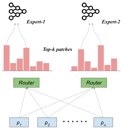
Appendix C Detailed results on deferred masking and patch mixer ablation study

When ablating the learning rate, we observe better performance with higher learning rates. However, we run into training instabilities after approximately $2$K steps, despite using qk-normalization (Dehghani et al., 2023), with mixed precision training. Overall, we recommend ablating the choice of learning rate for each network and using the maximum attainable value without causing training instability. We also consider a fast training strategy using cyclic learning schedules (Smith, 2015). Cyclic learning has been previously observed to improve the convergence rate for image classifiers (Smith, 2015; 2022). We consider a cyclic cosine schedule with base cycle time $t$ and each subsequent cycle duration multiplied by a multiplier ($m_{t}$). We only observe a marginal benefit of cyclic schedules (Table 11(g)). In favor of simplicity, we continue to use a single cycle schedule.

In ablating the choice of masking, we shift from masking patches randomly to retaining a continuous region of image patches with block masking 5(b). We perform this ablation on $256\times 256$ image resolution with a corresponding latent resolution of $32\times 32$ and $256$ patches with a patch size of two in the DiT-Tiny/2 model. Note that at a block size of 8 and a $75$% masking ratio, block sampling collapses to masking quadrants of image patches. Thus, for this configuration, we resort to sampling a single continuous square patch of non-masked patches. Overall, we find that any amount of block masking degrades performance compared to random masking of each patch. It is likely because despite latent compression and patching, there exists some redundancy in visual information between neighboring patches, and the diffusion transformer model receives more global semantic information about the image with random masking.

(a) a photo of a cow

(b) a photo of a cake and a zebra

(c) a photo of three buses

(d) a photo of a red potted plant

(e) a photo of an elephant below a surfboard

(f) a photo of an orange cow and a purple sandwich

Figure 13: Generation from a model trained only on real data (on left) and combined real and synthetic data (on right) on GenEval benchmark prompts. Both models use identical random seed for generation.

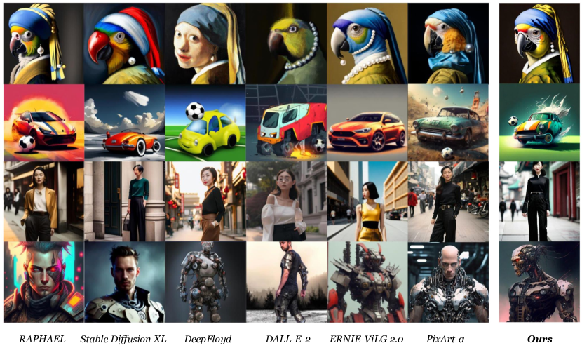
• A parrot with a pearl earring, Vermeer style.

• A car playing soccer, digital art.

• Street shot of a fashionable Chinese lady in Shanghai, wearing black high-waisted trousers.

• Half human, half robot, repaired human, human flesh warrior, mech display, man in mech, cyberpunk.

Figure 14: Comparison with previous works. Figure adapted from Chen et al. (2023).

(a) Previous works: RAPHAEL, Stable Diffusion XL, DeepFloyd, DALL-E-2, ERNIE-ViLG 2.0, PixArt-$\alpha$

(b) Our work

• A cute little matte low poly isometric cherry blossom forest island, waterfalls, lighting, soft shadows, trending on Artstation, 3d render, monument valley, fez video game.

• A shanty version of Tokyo, new rustic style, bold colors with all colors palette, video game, genshin, tribe, fantasy, overwatch.

• Cartoon characters, mini characters, figures, illustrations, flower fairy, green dress, brown hair,curly long hair, elf-like wings,many flowers and leaves, natural scenery, golden eyes, detailed light and shadow , a high degree of detail.

• Cartoon characters, mini characters, hand-made, illustrations, robotkids, color expressions, boy, short brown hair, curly hair,blue eyes, technological age, cyberpunk, big eyes, cute, mini, detailed light and shadow, high detail.

Figure 15: Comparison with previous works. Figure adapted from Chen et al. (2023).

Figure 16: Synthesized images by our model using randomly selected prompts from PartiPrompts (Yu et al., 2022). Rows correspond to following categories: Abstract, Animals, Artifacts, Arts, Food & Beverage, and Illustrations.

Figure 17: Synthesized images by our model using randomly selected prompts from PartiPrompts (Yu et al., 2022). Rows correspond to following categories: Indoor scenes, Outdoor scenes, People, Produce & Plants, Vehicles, and World knowledge.

Figure 18: Synthesized images by our model using randomly selected prompts from DrawBench (Saharia et al., 2022).

Figure 19: Synthesized images by our model using randomly selected prompts from GenEval (Ghosh et al., 2024).

(a) Stable-Diffusion-1.5

(b) Stable-Diffusion-2.1

(c) Stable-Diffusion-XL

(d) Ours

Figure 20: Evaluating the ability to generate diverse styles. Prompt: A   dressed in a suit posing for a photo in   style. Natural lake landscape in background, detailed light and shadow, high detail.

(a) Stable-Diffusion-1.5

(b) Stable-Diffusion-2.1

(c) Stable-Diffusion-XL

(d) Ours

Figure 21: Evaluating the ability to generate diverse styles. Prompt: A luxurious   with a next-generation modern design illustrated in   style.

(a) Stable-Diffusion-1.5

(b) Stable-Diffusion-2.1

(c) Stable-Diffusion-XL

(d) Ours

Figure 22: Evaluating the ability to generate diverse styles. Prompt: A moonlit night over a  , mysteriously rendered in   style.

(a) Stable-Diffusion-1.5

(b) Stable-Diffusion-2.1

(c) Stable-Diffusion-XL

(d) Ours

Figure 23: Evaluating the ability to generate diverse styles. Prompt: A lush garden full of  , vividly illustrated in   style.

Figure 24: Synthesized images by our model using randomly selected prompts from the test set of JourneyDB dataset (Ghosh et al., 2024).

Figure 25: Synthesized images by our model using randomly selected prompts from the test set of JourneyDB dataset (Ghosh et al., 2024).

Figure 26: Synthesized images by our model using randomly selected prompts from the test set of JourneyDB dataset (Ghosh et al., 2024).

Figure 27: Synthesized images by our model using randomly selected prompts from the test set of JourneyDB dataset (Ghosh et al., 2024).

Figure 28: Selected images with corresponding real and synthetic captions from the cifar-captions dataset. We created the cifar-captions dataset, imitating the widely used CIFAR-10 dataset (Krizhevsky et al., 2009), to enable small scale experimentation on the text-to-image generative models.

References

- Abdin et al. (2024) Marah Abdin, Sam Ade Jacobs, Ammar Ahmad Awan, Jyoti Aneja, Ahmed Awadallah, Hany Awadalla, Nguyen Bach, Amit Bahree, Arash Bakhtiari, Harkirat Behl, et al. Phi-3 technical report: A highly capable language model locally on your phone. arXiv preprint arXiv:2404.14219, 2024.
- Agarwal et al. (2022) Chirag Agarwal, Daniel D’souza, and Sara Hooker. Estimating example difficulty using variance of gradients. In Proceedings of the IEEE/CVF Conference on Computer Vision and Pattern Recognition, pp. 10368–10378, 2022.
- Balaji et al. (2022) Yogesh Balaji, Yogesh Balaji, Nah, Seungjun, Seungjun Nah, Huang, Xun, Xun Huang, Vahdat, Arash, Arash Vahdat, Song, Jiaming, Jiaming Song, Kreis, Karsten, Karsten Kreis, Aittala, Miika, Miika Aittala, Aila, Timo, Timo Aila, Laine, Samuli, Samuli Laine, Catanzaro, Bryan, Bryan Catanzaro, Karras, Tero, Tero Karras, Liu, Ming-Yu, and Mingyu Li. eDiff-I: Text-to-Image Diffusion Models with an Ensemble of Expert Denoisers. arXiv preprint arXiv:2211.01324, 2022. doi: 10.48550/arxiv.2211.01324.
- Bansal et al. (2024) Arpit Bansal, Eitan Borgnia, Hong-Min Chu, Jie Li, Hamid Kazemi, Furong Huang, Micah Goldblum, Jonas Geiping, and Tom Goldstein. Cold diffusion: Inverting arbitrary image transforms without noise. Advances in Neural Information Processing Systems, 36, 2024.
- Betker et al. (2023) James Betker, Gabriel Goh, Li Jing, Tim Brooks, Jianfeng Wang, Linjie Li, Long Ouyang, Juntang Zhuang, Joyce Lee, Yufei Guo, et al. Improving image generation with better captions. Computer Science. https://cdn. openai. com/papers/dall-e-3. pdf, 2(3):8, 2023.
- Brown et al. (2020) Tom Brown, Benjamin Mann, Nick Ryder, Melanie Subbiah, Jared D Kaplan, Prafulla Dhariwal, Arvind Neelakantan, Pranav Shyam, Girish Sastry, Amanda Askell, et al. Language models are few-shot learners. Advances in neural information processing systems, 33:1877–1901, 2020.
- Byeon et al. (2022) Minwoo Byeon, Beomhee Park, Haecheon Kim, Sungjun Lee, Woonhyuk Baek, and Saehoon Kim. Coyo-700m: Image-text pair dataset. https://github.com/kakaobrain/coyo-dataset, 2022.
- Changpinyo et al. (2021) Soravit Changpinyo, Piyush Sharma, Nan Ding, and Radu Soricut. Conceptual 12m: Pushing web-scale image-text pre-training to recognize long-tail visual concepts. In Proceedings of the IEEE/CVF conference on computer vision and pattern recognition, pp. 3558–3568, 2021.
- Chen et al. (2023) Jun Song Chen, Jincheng Yu, Chongjian Ge, Lewei Yao, Enze Xie, Yue Wu, Zhongdao Wang, James T. Kwok, Ping Luo, Huchuan Lu, and Zhenguo Li. PixArt-$\alpha$: Fast Training of Diffusion Transformer for Photorealistic Text-to-Image Synthesis. arXiv preprint arXiv:2310.00426, 2023. doi: 10.48550/arxiv.2310.00426.
- Choromanska et al. (2015) Anna Choromanska, Mikael Henaff, Michael Mathieu, Gérard Ben Arous, and Yann LeCun. The loss surfaces of multilayer networks. In Artificial intelligence and statistics, pp. 192–204. PMLR, 2015.
- Chou et al. (2023) Sheng-Yen Chou, Pin-Yu Chen, and Tsung-Yi Ho. How to backdoor diffusion models? In Proceedings of the IEEE/CVF Conference on Computer Vision and Pattern Recognition, pp. 4015–4024, 2023.
- Chowdhery et al. (2022) Aakanksha Chowdhery, Sharan Narang, Jacob Devlin, Maarten Bosma, Gaurav Mishra, Adam Roberts, Paul Barham, Hyung Won Chung, Charles Sutton, Sebastian Gehrmann, et al. Palm: Scaling language modeling with pathways. arxiv 2022. arXiv preprint arXiv:2204.02311, 10, 2022.
- Dai et al. (2023) Xiaoliang Dai, Ji Hou, Chih-Yao Ma, Sam Tsai, Jialiang Wang, Rui Wang, Peizhao Zhang, Simon Vandenhende, Xiaofang Wang, Abhimanyu Dubey, et al. Emu: Enhancing image generation models using photogenic needles in a haystack. arXiv preprint arXiv:2309.15807, 2023.
- Dai & Gifford (2023) Zheng Dai and David K Gifford. Training data attribution for diffusion models. arXiv preprint arXiv:2306.02174, 2023.
- Dehghani et al. (2023) Mostafa Dehghani, Josip Djolonga, Basil Mustafa, Piotr Padlewski, Jonathan Heek, Justin Gilmer, Andreas Peter Steiner, Mathilde Caron, Robert Geirhos, Ibrahim Alabdulmohsin, et al. Scaling vision transformers to 22 billion parameters. In International Conference on Machine Learning, pp. 7480–7512. PMLR, 2023.
- Deng et al. (2009) Jia Deng, Wei Dong, Richard Socher, Li-Jia Li, Kai Li, and Li Fei-Fei. Imagenet: A large-scale hierarchical image database. In 2009 IEEE conference on computer vision and pattern recognition, pp. 248–255. Ieee, 2009.
- Devlin et al. (2018) Jacob Devlin, Ming-Wei Chang, Kenton Lee, and Kristina Toutanova. Bert: Pre-training of deep bidirectional transformers for language understanding. arXiv preprint arXiv:1810.04805, 2018.
- Dhariwal & Nichol (2021) Prafulla Dhariwal and Alexander Nichol. Diffusion models beat gans on image synthesis. Advances in neural information processing systems, 34:8780–8794, 2021.
- Ding et al. (2022) Ming Ding, Wendi Zheng, Wenyi Hong, and Jie Tang. Cogview2: Faster and better text-to-image generation via hierarchical transformers. Advances in Neural Information Processing Systems, 35:16890–16902, 2022.
- Dosovitskiy et al. (2020) Alexey Dosovitskiy, Lucas Beyer, Alexander Kolesnikov, Dirk Weissenborn, Xiaohua Zhai, Thomas Unterthiner, Mostafa Dehghani, Matthias Minderer, Georg Heigold, Sylvain Gelly, et al. An image is worth 16x16 words: Transformers for image recognition at scale. In International Conference on Learning Representations, 2020.
- Esser et al. (2024) Patrick Esser, Sumith Kulal, Andreas Blattmann, Rahim Entezari, Jonas Müller, Harry Saini, Yam Levi, Dominik Lorenz, Axel Sauer, Frederic Boesel, et al. Scaling rectified flow transformers for high-resolution image synthesis. In Forty-first International Conference on Machine Learning, 2024.
- Fang et al. (2023) Alex Fang, Albin Madappally Jose, Amit Jain, Ludwig Schmidt, Alexander Toshev, and Vaishaal Shankar. Data filtering networks. arXiv preprint arXiv:2309.17425, 2023.
- Fedus et al. (2022) William Fedus, Barret Zoph, and Noam Shazeer. Switch transformers: Scaling to trillion parameter models with simple and efficient sparsity. Journal of Machine Learning Research, 23(120):1–39, 2022.
- Fourier (1822) Jean Baptiste Joseph Fourier. Théorie analytique de la chaleur, volume 504. Didot Paris, 1822.
- Gafni et al. (2022) Oran Gafni, Adam Polyak, Oron Ashual, Shelly Sheynin, Devi Parikh, and Yaniv Taigman. Make-a-scene: Scene-based text-to-image generation with human priors. In European Conference on Computer Vision, pp. 89–106. Springer, 2022.
- Gao et al. (2023) Shanghua Gao, Pan Zhou, Ming-Ming Cheng, and Shuicheng Yan. Mdtv2: Masked diffusion transformer is a strong image synthesizer. arXiv preprint arXiv:2303.14389, 2023.
- Ghosh et al. (2024) Dhruba Ghosh, Hannaneh Hajishirzi, and Ludwig Schmidt. Geneval: An object-focused framework for evaluating text-to-image alignment. Advances in Neural Information Processing Systems, 36, 2024.
- Gokaslan et al. (2024) Aaron Gokaslan, A Feder Cooper, Jasmine Collins, Landan Seguin, Austin Jacobson, Mihir Patel, Jonathan Frankle, Cory Stephenson, and Volodymyr Kuleshov. Commoncanvas: Open diffusion models trained on creative-commons images. In Proceedings of the IEEE/CVF Conference on Computer Vision and Pattern Recognition, pp. 8250–8260, 2024.
- Guo et al. (2024) Lanqing Guo, Yingqing He, Haoxin Chen, Menghan Xia, Xiaodong Cun, Yufei Wang, Siyu Huang, Yong Zhang, Xintao Wang, Qifeng Chen, Ying Shan, and Bihan Wen. Make a cheap scaling: A self-cascade diffusion model for higher-resolution adaptation, 2024. URL https://arxiv.org/abs/2402.10491.
- He et al. (2022) Kaiming He, Xinlei Chen, Saining Xie, Yanghao Li, Piotr Dollár, and Ross Girshick. Masked autoencoders are scalable vision learners. In Proceedings of the IEEE/CVF conference on computer vision and pattern recognition, pp. 16000–16009, 2022.
- Hendrycks & Gimpel (2016) Dan Hendrycks and Kevin Gimpel. Gaussian error linear units (gelus). arXiv preprint arXiv:1606.08415, 2016.
- Hessel et al. (2021) Jack Hessel, Ari Holtzman, Maxwell Forbes, Ronan Le Bras, and Yejin Choi. Clipscore: A reference-free evaluation metric for image captioning. arXiv preprint arXiv:2104.08718, 2021.
- Heusel et al. (2017) Martin Heusel, Hubert Ramsauer, Thomas Unterthiner, Bernhard Nessler, and Sepp Hochreiter. Gans trained by a two time-scale update rule converge to a local nash equilibrium. Advances in neural information processing systems, 30, 2017.
- Ho & Salimans (2022) Jonathan Ho and Tim Salimans. Classifier-free diffusion guidance. arXiv preprint arXiv:2207.12598, 2022.
- Ho et al. (2020) Jonathan Ho, Ajay Jain, and Pieter Abbeel. Denoising diffusion probabilistic models. Advances in neural information processing systems, 33:6840–6851, 2020.
- Ilharco et al. (2021) Gabriel Ilharco, Mitchell Wortsman, Ross Wightman, Cade Gordon, Nicholas Carlini, Rohan Taori, Achal Dave, Vaishaal Shankar, Hongseok Namkoong, John Miller, Hannaneh Hajishirzi, Ali Farhadi, and Ludwig Schmidt. Openclip, July 2021. URL https://doi.org/10.5281/zenodo.5143773.
- Jiang et al. (2023) Albert Q Jiang, Alexandre Sablayrolles, Arthur Mensch, Chris Bamford, Devendra Singh Chaplot, Diego de las Casas, Florian Bressand, Gianna Lengyel, Guillaume Lample, Lucile Saulnier, et al. Mistral 7b. arXiv preprint arXiv:2310.06825, 2023.
- Jiang et al. (2020) Yiding Jiang, Pierre Foret, Scott Yak, Daniel M Roy, Hossein Mobahi, Gintare Karolina Dziugaite, Samy Bengio, Suriya Gunasekar, Isabelle Guyon, and Behnam Neyshabur. Neurips 2020 competition: Predicting generalization in deep learning. arXiv preprint arXiv:2012.07976, 2020.
- Jolicoeur-Martineau et al. (2021) Alexia Jolicoeur-Martineau, Ke Li, Rémi Piché-Taillefer, Tal Kachman, and Ioannis Mitliagkas. Gotta go fast when generating data with score-based models. arXiv preprint arXiv:2105.14080, 2021.
- Kang et al. (2023) Minguk Kang, Jun-Yan Zhu, Richard Zhang, Jaesik Park, Eli Shechtman, Sylvain Paris, and Taesung Park. Scaling up gans for text-to-image synthesis. In Proceedings of the IEEE/CVF Conference on Computer Vision and Pattern Recognition, pp. 10124–10134, 2023.
- Karras et al. (2022) Tero Karras, Miika Aittala, Timo Aila, and Samuli Laine. Elucidating the design space of diffusion-based generative models, 2022.
- Karras et al. (2024) Tero Karras, Miika Aittala, Tuomas Kynkäänniemi, Jaakko Lehtinen, Timo Aila, and Samuli Laine. Guiding a diffusion model with a bad version of itself. arXiv preprint arXiv:2406.02507, 2024.
- Kim et al. (2021) Saehoon Kim, Sanghun Cho, Chiheon Kim, Doyup Lee, and Woonhyuk Baek. mindall-e on conceptual captions. https://github.com/kakaobrain/minDALL-E, 2021.
- Kirillov et al. (2023) Alexander Kirillov, Eric Mintun, Nikhila Ravi, Hanzi Mao, Chloe Rolland, Laura Gustafson, Tete Xiao, Spencer Whitehead, Alexander C Berg, Wan-Yen Lo, et al. Segment anything. In Proceedings of the IEEE/CVF International Conference on Computer Vision, pp. 4015–4026, 2023.
- Koh & Liang (2017) Pang Wei Koh and Percy Liang. Understanding black-box predictions via influence functions. In International conference on machine learning, pp. 1885–1894. PMLR, 2017.
- Krizhevsky et al. (2009) Alex Krizhevsky, Geoffrey Hinton, et al. Learning multiple layers of features from tiny images. 2009.
- Li et al. (2024) Xianhang Li, Haoqin Tu, Mude Hui, Zeyu Wang, Bingchen Zhao, Junfei Xiao, Sucheng Ren, Jieru Mei, Qing Liu, Huangjie Zheng, et al. What if we recaption billions of web images with llama-3? arXiv preprint arXiv:2406.08478, 2024.
- Lin et al. (2014) Tsung-Yi Lin, Michael Maire, Serge Belongie, James Hays, Pietro Perona, Deva Ramanan, Piotr Dollár, and C Lawrence Zitnick. Microsoft coco: Common objects in context. In Computer Vision–ECCV 2014: 13th European Conference, Zurich, Switzerland, September 6-12, 2014, Proceedings, Part V 13, pp. 740–755. Springer, 2014.
- Liu et al. (2023) Haotian Liu, Chunyuan Li, Yuheng Li, and Yong Jae Lee. Improved baselines with visual instruction tuning. arXiv preprint arXiv:2310.03744, 2023.
- Liu et al. (2022) Luping Liu, Yi Ren, Zhijie Lin, and Zhou Zhao. Pseudo numerical methods for diffusion models on manifolds. arXiv preprint arXiv:2202.09778, 2022.
- Mehta et al. (2024) Sachin Mehta, Mohammad Hossein Sekhavat, Qingqing Cao, Maxwell Horton, Yanzi Jin, Chenfan Sun, Iman Mirzadeh, Mahyar Najibi, Dmitry Belenko, Peter Zatloukal, et al. Openelm: An efficient language model family with open-source training and inference framework. arXiv preprint arXiv:2404.14619, 2024.
- Mellempudi et al. (2019) Naveen Mellempudi, Sudarshan Srinivasan, Dipankar Das, and Bharat Kaul. Mixed precision training with 8-bit floating point. arXiv preprint arXiv:1905.12334, 2019.
- Nichol et al. (2021) Alex Nichol, Prafulla Dhariwal, Aditya Ramesh, Pranav Shyam, Pamela Mishkin, Bob McGrew, Ilya Sutskever, and Mark Chen. Glide: Towards photorealistic image generation and editing with text-guided diffusion models. arXiv preprint arXiv:2112.10741, 2021.
- OpenAI (2024) OpenAI. Hello gpt-4o. https://openai.com/index/hello-gpt-4o/, 2024.
- Park et al. (2023) Sung Min Park, Kristian Georgiev, Andrew Ilyas, Guillaume Leclerc, and Aleksander Madry. Trak: Attributing model behavior at scale. arXiv preprint arXiv:2303.14186, 2023.
- Parmar et al. (2022) Gaurav Parmar, Richard Zhang, and Jun-Yan Zhu. On aliased resizing and surprising subtleties in gan evaluation. In Proceedings of the IEEE/CVF Conference on Computer Vision and Pattern Recognition, pp. 11410–11420, 2022.
- Paszke et al. (2019) Adam Paszke, Sam Gross, Francisco Massa, Adam Lerer, James Bradbury, Gregory Chanan, Trevor Killeen, Zeming Lin, Natalia Gimelshein, Luca Antiga, et al. Pytorch: An imperative style, high-performance deep learning library. Advances in neural information processing systems, 32, 2019.
- Peebles & Xie (2023) William Peebles and Saining Xie. Scalable diffusion models with transformers. In Proceedings of the IEEE/CVF International Conference on Computer Vision, pp. 4195–4205, 2023.
- Pernias et al. (2024) Pablo Pernias, Dominic Rampas, Mats L. Richter, Christopher J. Pal, and Marc Aubreville. Wuerstchen: An Efficient Architecture for Large-Scale Text-to-Image Diffusion Models. ICLR, 2024.
- Podell et al. (2024) Dustin Podell, Zion English, Karen Lacey, Andreas Blattmann, Tim Dockhorn, Judith Müller, Joe Penna, and Robin Rombach. SDXL: Improving Latent Diffusion Models for High-Resolution Image Synthesis. ICLR, 2024. doi: 10.48550/arxiv.2307.01952.
- Radford et al. (2021) Alec Radford, Jong Wook Kim, Chris Hallacy, Aditya Ramesh, Gabriel Goh, Sandhini Agarwal, Girish Sastry, Amanda Askell, Pamela Mishkin, Jack Clark, et al. Learning transferable visual models from natural language supervision. In International conference on machine learning, pp. 8748–8763. PMLR, 2021.
- Raffel et al. (2020) Colin Raffel, Noam Shazeer, Adam Roberts, Katherine Lee, Sharan Narang, Michael Matena, Yanqi Zhou, Wei Li, and Peter J Liu. Exploring the limits of transfer learning with a unified text-to-text transformer. Journal of machine learning research, 21(140):1–67, 2020.
- Ramesh et al. (2021) Aditya Ramesh, Mikhail Pavlov, Gabriel Goh, Scott Gray, Chelsea Voss, Alec Radford, Mark Chen, and Ilya Sutskever. Zero-shot text-to-image generation. In International conference on machine learning, pp. 8821–8831. Pmlr, 2021.
- Ramesh et al. (2022) Aditya Ramesh, Prafulla Dhariwal, Alex Nichol, Casey Chu, and Mark Chen. Hierarchical text-conditional image generation with clip latents. arXiv preprint arXiv:2204.06125, 1(2):3, 2022.
- Rasley et al. (2020) Jeff Rasley, Samyam Rajbhandari, Olatunji Ruwase, and Yuxiong He. Deepspeed: System optimizations enable training deep learning models with over 100 billion parameters. In Proceedings of the 26th ACM SIGKDD International Conference on Knowledge Discovery & Data Mining, pp. 3505–3506, 2020.
- Rombach et al. (2022) Robin Rombach, Andreas Blattmann, Dominik Lorenz, Patrick Esser, and Björn Ommer. High-resolution image synthesis with latent diffusion models. In Proceedings of the IEEE/CVF conference on computer vision and pattern recognition, pp. 10684–10695, 2022.
- Saharia et al. (2022) Chitwan Saharia, William Chan, Saurabh Saxena, Lala Li, Jay Whang, Emily L Denton, Kamyar Ghasemipour, Raphael Gontijo Lopes, Burcu Karagol Ayan, Tim Salimans, et al. Photorealistic text-to-image diffusion models with deep language understanding. Advances in neural information processing systems, 35:36479–36494, 2022.
- Sanchez et al. (2023) Guillaume Sanchez, Honglu Fan, Alexander Spangher, Elad Levi, Pawan Sasanka Ammanamanchi, and Stella Biderman. Stay on topic with classifier-free guidance. arXiv preprint arXiv:2306.17806, 2023.
- Sauer et al. (2023) Axel Sauer, Dominik Lorenz, Andreas Blattmann, and Robin Rombach. Adversarial diffusion distillation. arXiv preprint arXiv:2311.17042, 2023.
- Schuhmann et al. (2022) Christoph Schuhmann, Romain Beaumont, Richard Vencu, Cade Gordon, Ross Wightman, Mehdi Cherti, Theo Coombes, Aarush Katta, Clayton Mullis, Mitchell Wortsman, et al. Laion-5b: An open large-scale dataset for training next generation image-text models. Advances in Neural Information Processing Systems, 35:25278–25294, 2022.
- Sehwag et al. (2022) Vikash Sehwag, Caner Hazirbas, Albert Gordo, Firat Ozgenel, and Cristian Canton. Generating high fidelity data from low-density regions using diffusion models. In Proceedings of the IEEE/CVF Conference on Computer Vision and Pattern Recognition, pp. 11492–11501, 2022.
- Shafahi et al. (2018) Ali Shafahi, W Ronny Huang, Mahyar Najibi, Octavian Suciu, Christoph Studer, Tudor Dumitras, and Tom Goldstein. Poison frogs! targeted clean-label poisoning attacks on neural networks. Advances in neural information processing systems, 31, 2018.
- Shah et al. (2024) Jay Shah, Ganesh Bikshandi, Ying Zhang, Vijay Thakkar, Pradeep Ramani, and Tri Dao. Flashattention-3: Fast and accurate attention with asynchrony and low-precision, 2024. URL https://arxiv.org/abs/2407.08608.
- Shazeer (2020) Noam Shazeer. Glu variants improve transformer. arXiv preprint arXiv:2002.05202, 2020.
- Shazeer et al. (2017) Noam Shazeer, Azalia Mirhoseini, Krzysztof Maziarz, Andy Davis, Quoc Le, Geoffrey Hinton, and Jeff Dean. Outrageously large neural networks: The sparsely-gated mixture-of-experts layer. arXiv preprint arXiv:1701.06538, 2017.
- Sidorov et al. (2020) Oleksii Sidorov, Ronghang Hu, Marcus Rohrbach, and Amanpreet Singh. Textcaps: a dataset for image captioning with reading comprehension. In Computer Vision–ECCV 2020: 16th European Conference, Glasgow, UK, August 23–28, 2020, Proceedings, Part II 16, pp. 742–758. Springer, 2020.
- Smith (2015) Leslie N Smith. Cyclical learning rates for training neural networks. arxiv. Preprint at https://arxiv. org/abs/1506.01186, 2015.
- Smith (2022) Leslie N Smith. General cyclical training of neural networks. arXiv preprint arXiv:2202.08835, 2022.
- Sohl-Dickstein et al. (2015) Jascha Sohl-Dickstein, Eric Weiss, Niru Maheswaranathan, and Surya Ganguli. Deep unsupervised learning using nonequilibrium thermodynamics. In International conference on machine learning, pp. 2256–2265. PMLR, 2015.
- Song et al. (2020a) Jiaming Song, Chenlin Meng, and Stefano Ermon. Denoising diffusion implicit models. arXiv preprint arXiv:2010.02502, 2020a.
- Song et al. (2020b) Yang Song, Jascha Sohl-Dickstein, Diederik P Kingma, Abhishek Kumar, Stefano Ermon, and Ben Poole. Score-based generative modeling through stochastic differential equations. arXiv preprint arXiv:2011.13456, 2020b.
- Song et al. (2021) Yang Song, Jascha Sohl-Dickstein, Diederik P Kingma, Abhishek Kumar, Stefano Ermon, and Ben Poole. Score-based generative modeling through stochastic differential equations. ICLR, 2021.
- Song et al. (2023) Yang Song, Prafulla Dhariwal, Mark Chen, and Ilya Sutskever. Consistency models. arXiv preprint arXiv:2303.01469, 2023.
- Sun et al. (2024) Keqiang Sun, Junting Pan, Yuying Ge, Hao Li, Haodong Duan, Xiaoshi Wu, Renrui Zhang, Aojun Zhou, Zipeng Qin, Yi Wang, et al. Journeydb: A benchmark for generative image understanding. Advances in Neural Information Processing Systems, 36, 2024.
- Sutawika et al. (2024) Lintang Sutawika, Aran Komatsuzaki, and Colin Raffel. Pile-t5, 2024. URL https://blog.eleuther.ai/pile-t5/. Blog post.
- Szegedy et al. (2016) Christian Szegedy, Vincent Vanhoucke, Sergey Ioffe, Jon Shlens, and Zbigniew Wojna. Rethinking the inception architecture for computer vision. In Proceedings of the IEEE conference on computer vision and pattern recognition, pp. 2818–2826, 2016.
- Team (2022) Mosaic ML Team. streaming. <https://github.com/mosaicml/streaming/>, 2022.
- Teng et al. (2023) Jiayan Teng, Wendi Zheng, Ming Ding, Wenyi Hong, Jianqiao Wangni, Zhuoyi Yang, and Jie Tang. Relay diffusion: Unifying diffusion process across resolutions for image synthesis. arXiv preprint arXiv:2309.03350, 2023.
- Touvron et al. (2023) Hugo Touvron, Thibaut Lavril, Gautier Izacard, Xavier Martinet, Marie-Anne Lachaux, Timothée Lacroix, Baptiste Rozière, Naman Goyal, Eric Hambro, Faisal Azhar, et al. Llama: Open and efficient foundation language models. arXiv preprint arXiv:2302.13971, 2023.
- Valyaeva (2023) Alina Valyaeva. AI Has Already Created As Many Images As Photographers Have Taken in 150 Years. Statistics for 2023. https://journal.everypixel.com/ai-image-statistics, 2023. [Online; accessed 11-July-2024].
- Vaswani et al. (2017) Ashish Vaswani, Noam Shazeer, Niki Parmar, Jakob Uszkoreit, Llion Jones, Aidan N Gomez, Łukasz Kaiser, and Illia Polosukhin. Attention is all you need. Advances in neural information processing systems, 30, 2017.
- Wang et al. (2023) Weihan Wang, Qingsong Lv, Wenmeng Yu, Wenyi Hong, Ji Qi, Yan Wang, Junhui Ji, Zhuoyi Yang, Lei Zhao, Xixuan Song, et al. Cogvlm: Visual expert for pretrained language models. arXiv preprint arXiv:2311.03079, 2023.
- Wang et al. (2022) Zijie J Wang, Evan Montoya, David Munechika, Haoyang Yang, Benjamin Hoover, and Duen Horng Chau. Diffusiondb: A large-scale prompt gallery dataset for text-to-image generative models. arXiv preprint arXiv:2210.14896, 2022.
- Xie et al. (2024) Sang Michael Xie, Hieu Pham, Xuanyi Dong, Nan Du, Hanxiao Liu, Yifeng Lu, Percy S Liang, Quoc V Le, Tengyu Ma, and Adams Wei Yu. Doremi: Optimizing data mixtures speeds up language model pretraining. Advances in Neural Information Processing Systems, 36, 2024.
- Yariv et al. (2023) Guy Yariv, Itai Gat, Lior Wolf, Yossi Adi, and Idan Schwartz. Audiotoken: Adaptation of text-conditioned diffusion models for audio-to-image generation. arXiv preprint arXiv:2305.13050, 2023.
- Yu et al. (2022) Jiahui Yu, Yuanzhong Xu, Jing Yu Koh, Thang Luong, Gunjan Baid, Zirui Wang, Vijay Vasudevan, Alexander Ku, Yinfei Yang, Burcu Karagol Ayan, et al. Scaling autoregressive models for content-rich text-to-image generation. Transactions on Machine Learning Research, 2022.
- Zeiler & Fergus (2014) Matthew D Zeiler and Rob Fergus. Visualizing and understanding convolutional networks. In Computer Vision–ECCV 2014: 13th European Conference, Zurich, Switzerland, September 6-12, 2014, Proceedings, Part I 13, pp. 818–833. Springer, 2014.
- Zhang et al. (2023) Lvmin Zhang, Anyi Rao, and Maneesh Agrawala. Adding conditional control to text-to-image diffusion models. In Proceedings of the IEEE/CVF International Conference on Computer Vision, pp. 3836–3847, 2023.
- Zhao et al. (2024) Linxi Zhao, Yihe Deng, Weitong Zhang, and Quanquan Gu. Mitigating object hallucination in large vision-language models via classifier-free guidance. arXiv preprint arXiv:2402.08680, 2024.
- Zheng et al. (2024) Hongkai Zheng, Weili Nie, Arash Vahdat, and Anima Anandkumar. Fast training of diffusion models with masked transformers. Transactions on Machine Learning Research, 2024. ISSN 2835-8856. URL https://openreview.net/forum?id=vTBjBtGioE.
- Zheng et al. (2023) Xiaosen Zheng, Tianyu Pang, Chao Du, Jing Jiang, and Min Lin. Intriguing properties of data attribution on diffusion models. arXiv preprint arXiv:2311.00500, 2023.
- Zhou et al. (2022) Yanqi Zhou, Tao Lei, Hanxiao Liu, Nan Du, Yanping Huang, Vincent Zhao, Andrew M Dai, Quoc V Le, James Laudon, et al. Mixture-of-experts with expert choice routing. Advances in Neural Information Processing Systems, 35:7103–7114, 2022.
- Zoph et al. (2022) Barret Zoph, Irwan Bello, Sameer Kumar, Nan Du, Yanping Huang, Jeff Dean, Noam Shazeer, and William Fedus. St-moe: Designing stable and transferable sparse expert models. arXiv preprint arXiv:2202.08906, 2022.