Coupled phantom cosmological model motivated by the warm inflationary paradigm

Abstract

In this article, we investigate a coupled phantom dark-energy cosmological model in which the coupling term between a phantom scalar field with an exponential potential and a pressureless dark-matter fluid is motivated by the warm inflationary paradigm. Using methods of qualitative analysis of dynamical systems, complemented by numerical solutions of the evolution equations, we study the late-time behavior of our model. We show that contrary to the uncoupled scenario, the coupled phantom model admits accelerated scaling solutions. However, they do not correspond to a final state of the universe’s evolution and, therefore, cannot be used to solve the cosmological coincidence problem. Furthermore, we show that, for certain coupling parameter values, the total equation-of-state parameter’s asymptotic behavior is significantly changed when compared to the uncoupled scenario, allowing for solutions less phantom even for steeper potentials of the phantom scalar field.

I Introduction

Modern cosmology has received tremendous attention from the scientific community due to the availability of a large number of astronomical probes. The discovery of the cosmic microwave background radiation Penzias and Wilson (1965) demanded a theory for our early universe, and inflation Guth (1981); Linde (1982) — an accelerating expansion of the universe during its early time — served as a potential proposal for explaining a number of early universe puzzles. At the end of the 1990s, Supernovae Type Ia observations revealed that our universe is presently experiencing another phase of accelerating expansion Riess et al. (1998); Perlmutter et al. (1999). This late accelerating expansion was further confirmed by other complementary observations Astier and Pain (2012), and as a consequence, a theory for describing this phenomenon became essential.

To explain the present-day accelerating expansion of the universe, two common approaches are usually put forward. One is the introduction of some hypothetical dark energy (DE) fluid with large negative pressure in the context of Einstein’s General Relativity (GR) Peebles and Ratra (2003); Copeland et al. (2006); Sahni and Starobinsky (2006); Bamba et al. (2012). Alternatively, modifying GR or introducing new gravitational theories beyond GR in various ways can explain this late-time accelerating expansion; such models are widely known as modified gravity (MG) models Nojiri and Odintsov (2007, 2011); De Felice and Tsujikawa (2010); Capozziello and De Laurentis (2011); Clifton et al. (2012); Koyama (2016); Cai et al. (2016); Nojiri et al. (2017); Bahamonde et al. (2023) and sometimes the resulting fluid in this sector mimicking the behavior of DE is known as geometrical DE. The concepts of DE and MG introduced plenty of cosmological models in the literature, which have been widely investigated with various astronomical probes Peebles and Ratra (2003); Copeland et al. (2006); Sahni and Starobinsky (2006); Bamba et al. (2012); Nojiri and Odintsov (2007, 2011); De Felice and Tsujikawa (2010); Capozziello and De Laurentis (2011); Clifton et al. (2012); Koyama (2016); Cai et al. (2016); Nojiri et al. (2017); Bahamonde et al. (2023). However, based on up-to-date observational evidences, the actual reason for this accelerating expansion — DE, geometrical DE, or any other alternatives — is not yet known. Additionally, a significant amount of non-luminous dark matter (DM), which is responsible for structure formation, exists in our universe. A small amount of the total energy density ($\sim 4\%$) is contributed by baryons, photons, and neutrinos. Thus, the dynamics of our universe is dominated mainly by DM and DE (geometrical DE). Now, when considering a wide variety of cosmological scenarios accounting for both DM and DE (or geometrical DE), a large span of observational data is in favor of a simple cosmological scenario constructed within the context of GR plus a positive cosmological constant $\Lambda$, the so-called $\Lambda$CDM cosmological model. In this model, DM is a pressureless nonrelativistic fluid (i.e., cold DM abbreviated as CDM) and $\Lambda$ serves as DE. Additionally, in this cosmological setup, DE and DM each have their own conservation equations, meaning that they evolve independently with the expansion of the universe. However, $\Lambda$CDM has faced some challenges in the past, such as the cosmological constant problem Weinberg (1989) and the cosmic coincidence problem Zlatev et al. (1999). Furthermore, according to recent observational data, cosmological tensions are also challenging the standard $\Lambda$CDM model, leading to the argument that this model is probably an approximate version of a more realistic theory which is not yet known Abdalla et al. (2022). Thus, an extension of the $\Lambda$CDM cosmology is welcome in order to tackle these problems.

One of the generalizations of the $\Lambda$CDM cosmology is the theory of interacting DE or coupled DE where an interaction (i.e., energy exchange mechanism) between DM and DE is allowed. Interacting cosmologies have many attractive consequences, e.g., the alleviation of the cosmic coincidence problem Amendola (2000); Cai and Wang (2005); Pavon and Zimdahl (2005); Huey and Wandelt (2006); del Campo et al. (2008, 2009), phantom crossing Wang et al. (2005); Das et al. (2006); Sadjadi and Honardoost (2007); Pan and Chakraborty (2014), and reconciling the cosmological tensions Kumar and Nunes (2017); Di Valentino et al. (2017); Yang et al. (2018a); Pan et al. (2019); Pourtsidou and Tram (2016); An et al. (2018); Kumar et al. (2019). The above interesting outcomes motivated many researchers to work on interacting cosmologies, and since the beginning of the 21st century to the present date, a multitude of interacting cosmological models have been studied Amendola (2000); Cai and Wang (2005); Yang et al. (2018a); Pan et al. (2019); Barrow and Clifton (2006); Valiviita et al. (2008); Henriques et al. (2009); Gavela et al. (2009); Valiviita et al. (2010); Cao et al. (2011); He et al. (2011); Yang and Xu (2014a); Li and Zhang (2014); Yang and Xu (2014b, c); Pan et al. (2015); Nunes et al. (2016); Yang et al. (2016, 2017a, 2017b); Mifsud and Van De Bruck (2017); Yang et al. (2017c, 2018b, 2018c); Pan et al. (2020a); Sá (2020a); Pan et al. (2020b); Sá (2020b); Di Valentino et al. (2020, 2021); Sá (2021); Gao et al. (2021); Yang et al. (2021); Lucca (2021); Potting and Sá (2022); Chatzidakis et al. (2022); Zhai et al. (2023); Li and Zhang (2023); Teixeira et al. (2023); Sá (2023); Giarè et al. (2024a); Halder et al. (2024); Giarè et al. (2024b). The heart of interacting cosmologies is the coupling function or the interaction rate (also known as the interaction function) that controls the energy flow between the dark sectors. As the interaction function modifies the evolution of the dark components at the background and perturbation levels, the choice of the interaction function is of great importance.

In the present article, we consider an interacting scenario between a phantom DE scalar field and a pressureless DM fluid in which the interaction is motivated by the warm inflationary paradigm. We analyzed such a model using dynamical system techniques.

According to the warm-inflationary paradigm Berera (1995) (see also Berera (2023)), energy is continuously transferred from an inflaton field $\psi$ to a radiation bath, and hence, the energy density of the radiation sector, $\rho_{\texttt{R}}$, is not thinned out during the inflationary expansion. As a result of this energy transfer, a post-inflationary radiation-dominated phase is found without the need for a reheating period, which is essential in the standard inflationary scenario Guth (1981); Linde (1982). Therefore, in the warm inflationary paradigm, assuming the well-known Friedmann-Lemaître-Robertson-Walker (FLRW) geometry for the background, the evolution equations for the inflaton field and the radiation sector require a dissipative term as follows,

$$\dot{\psi}\ddot{\psi}+3H\dot{\psi}^{2}+\frac{\partial V}{\partial\psi}\dot{\psi} =-\Gamma\dot{\psi}^{2},$$ (1)

$$\dot{\rho}_{\texttt{R}}+4H\rho_{\texttt{R}} =\Gamma\dot{\psi}^{2},$$ (2)

where $H$ is the Hubble parameter, $V=V(\psi)$ denotes the potential of the inflaton field, and $\Gamma$ is the dissipation coefficient. In general, $\Gamma$ might be a function of the inflaton field and the temperature $T$ of the radiation bath, meaning that $\Gamma=\Gamma(\psi,T)$. The warm-inflationary paradigm has received considerable attention from the scientific community with both positive and negative comments (see Ref. Berera (2023) and the references therein). Since most cosmological theories have been challenged, and this reveals indeed a fruitful progress of science, we avoid the criticisms on warm inflation and focus ourselves, in the present work, on the interacting dynamics in which the interaction function finds its motivation in the warm inflationary theory.

This article is organized as follows. In section II, we provide a detailed review of the uncoupled phantom DE cosmological model. Then, in section III, we present our coupled phantom DE cosmological model, in which the interaction term between DE and DM is inspired by the warm inflationary paradigm. For this model, we carry out a thorough dynamical system analysis and present the results. Finally, in section IV, we conclude the article by highlighting the key findings.

II Uncoupled phantom dark energy

In this section, the uncoupled phantom DE cosmological model is briefly reviewed (for more details, see Caldwell (2002); Schulz and White (2001); Gibbons (2003); Li and Hao (2004); Hao and Li (2004); Chimento and Lazkoz (2003); Vikman (2005); Ludwick (2017) and the references therein).

The FLRW metric takes the form

$$ds^{2}=-dt^{2}+a^{2}(t)\left[\frac{dr^{2}}{1-kr^{2}}+r^{2}(d\theta^{2}+\sin^{2}\theta d\phi^{2})\right],$$ (3)

where $a(t)$ denotes the scale factor and $k=0,1,-1$ is a constant representing the curvature of the space (flat, closed, or open, respectively). In this work, we consider a flat FLRW universe, i.e., we set $k=0$.

We further assume that the gravitational sector of the universe is described by Einstein’s General Relativity (GR) and the matter sector, minimally coupled to gravity, comprises a pressureless DM fluid with energy density $\rho_{\rm DM}$ and a phantom DE scalar field $\phi$ with an exponential potential

$$V(\phi)=V_{0}e^{-\lambda\kappa\phi},$$ (4)

where $V_{0}$ and $\lambda$ are positive constants of dimension (mass)⁴ and (mass)⁰, respectively, and the notation $\kappa\equiv\sqrt{8\pi G}=\sqrt{8\pi}/m_{p}$ (here $m_{p}$ stands for the Planck mass) has been used. We neglect radiation and baryons and their influence on the universe’s late-time evolution.

Under the above assumptions, the evolution equations for the uncoupled phantom DE cosmological model become

$$H^{2}=\frac{\kappa^{2}}{3}\left(-\frac{\dot{\phi}^{2}}{2}+V(\phi)+\rho_{\rm DM}\right),$$ (5)

$$\dot{H}=-\frac{\kappa^{2}}{2}\left(-\dot{\phi}^{2}+\rho_{\rm DM}\right),$$ (6)

$$\ddot{\phi}+3H\dot{\phi}-\frac{\partial V(\phi)}{\partial\phi}=0,$$ (7)

$$\dot{\rho}_{\rm DM}+3H\rho_{\rm DM}=0,$$ (8)

where $H=\dot{a}/a$ is the Hubble parameter, an overdot denotes a derivative with respect to cosmic time $t$, and the energy density and pressure of the phantom scalar field are given by

$$\rho_{\phi}=-\frac{\dot{\phi}^{2}}{2}+V(\phi)\quad\mbox{and}\quad p_{\phi}=-\frac{\dot{\phi}^{2}}{2}-V(\phi),$$ (9)

respectively.

Introducing the dimensionless variables

$$x=\frac{\kappa\dot{\phi}}{\sqrt{6}H}\quad\mbox{and}\quad y=\frac{\kappa\sqrt{V}}{\sqrt{3}H},$$ (10)

and a new time variable $\eta$, defined as

$$\frac{d\eta}{dt}=H,$$ (11)

the above evolution equations yield the two-dimensional autonomous dynamical system

$$x_{\eta}= -\frac{\sqrt{6}}{2}\lambda y^{2}-\frac{3}{2}x\left(1+x^{2}+y^{2}\right),$$ (12a)

$$y_{\eta}= \left[-\frac{\sqrt{6}}{2}\lambda x+\frac{3}{2}\left(1-x^{2}-y^{2}\right)\right]y,$$ (12b)

where the subscript $\eta$ denotes the derivative with respect to $\eta=\ln(a/a_{0})$, $a_{0}$ refers to the present value of the scale factor, and, without any loss of generality, we can set $a_{0}=1$. Note that the variable $\eta$ is nothing more than the number of $e$-folds $N$, a convenient measure of the expansion of the universe.

From the Friedmann equation (5), the DM density parameter $\Omega_{\rm DM}$, defined as the ratio between $\rho_{\rm DM}$ and the critical density $3H^{2}/\kappa^{2}$, can be expressed in terms of the dimensionless variables $x$ and $y$ as

$$\Omega_{\rm DM}=1+x^{2}-y^{2},$$ (13)

and hence, the DE density parameter, defined as $\Omega_{\phi}=\kappa^{2}\rho_{\phi}/3H^{2}$, can be expressed as

$$\Omega_{\phi}=-x^{2}+y^{2}=1-\Omega_{\rm DM}.$$ (14)

Taking into account that the energy density and the pressure of the phantom scalar field are given by Eq. (9), the phantom equation-of-state parameter $w_{\phi}=p_{\phi}/\rho_{\phi}$ and the total equation-of-state parameter $w_{\rm tot}=(p_{\phi}+p_{\rm DM})/(\rho_{\phi}+\rho_{\rm DM})$ can be expressed in terms of the dimensionless variables $x$ and $y$ as

$$w_{\phi} =\frac{x^{2}+y^{2}}{x^{2}-y^{2}},$$ (15)

$$w_{\rm tot} =-(x^{2}+y^{2}).$$ (16)

Using the dynamical system (12), the evolution equation for the DM density parameter can be written as

$$\Omega_{{\rm DM},\eta}=-3\left(x^{2}+y^{2}\right)\Omega_{\rm DM},$$ (17)

implying that the hyperbolas $y=\pm\sqrt{1+x^{2}}$ are invariant manifolds, i.e., they are not crossed by phase-space orbits. Inspection of Eq. (12b) further reveals that $y=0$ is also an invariant manifold. Since $\Omega_{\rm DM}$ is non-negative by definition ($y^{2}\leq 1+x^{2}$) and we are interested in non-contracting cosmological solutions ($y\geq 0$), the phase space of the dynamical system (12) is given by

$$R_{2}=\left\{(x,y)\in\mathbb{R}^{2}:y\leq\sqrt{1+x^{2}},y\geq 0\right\}.$$ (18)

Note that the phantom equation-of-state parameter (15) becomes infinite for $y^{2}=x^{2}$. This is a direct consequence of the fact that, due to the negative sign in the kinetic-energy term, the total energy of the scalar field is no longer bounded from below, implying, from a quantum point of view, the appearance of ghosts in the theory, and, from a classical perspective, the instability of the equation-of-motion solutions under small perturbations Carroll et al. (2003). After analyzing the stability of the critical points of the dynamical system (12) and describing the phase-space orbits, we shall return to this issue.

The dynamical system (12), in the finite region of the phase space, has just two critical points, $A_{0}$ and $A_{1}$. Their properties (existence, eigenvalues, stability, and various cosmological features) are highlighted in Table 1.

Critical point	Existence	Eigenvalues	Stability	$\Omega_{\phi}$	$\Omega_{\rm DM}$	$w_{\rm tot}$	Acceleration
$A_{0}(0,0)$	Always	$\left(-\frac{3}{2},\frac{3}{2}\right)$	Saddle	0	1	0	Never
$A_{1}\left(-\frac{\lambda}{\sqrt{6}},\sqrt{1+\frac{\lambda^{2}}{6}}\right)$	Always	$\left(-3-\lambda^{2},-3-\frac{\lambda^{2}}{2}\right)$	Attractor	1	0	$-1-\frac{\lambda^{2}}{3}$	Always

Table 1: Critical points of the dynamical system (12) and their properties for the uncoupled phantom DE cosmological model.

The critical point $A_{0}$ is located at the origin $(0,0)$ of the phase space and always exists independently of the $\lambda$ parameter’s value. It represents a matter-dominated cosmological solution ($\Omega_{\rm DM}=1$) with decelerated expansion ($w_{\rm tot}=0$). Since the eigenvalues of the Jacobian matrix of the dynamical system (12) are nonzero and have opposite signs, linear stability theory indicates that $A_{0}$ is a saddle point. In summary, this critical point corresponds to a DM-dominated decelerated phase of the universe’s evolution.

The critical point $A_{1}$ also exists for any value of the parameter $\lambda$. It lies on the hyperbola $y=\sqrt{1+x^{2}}$ and represents a solution completely dominated by DE ($\Omega_{\phi}=1$). Because $w_{\rm tot}<-1/3$ for any value of $\lambda$, it always corresponds to an accelerating solution. Since both the eigenvalues are negative, $A_{1}$ is a global attractor. Therefore, this critical point corresponds to a DE-dominated late-time accelerating solution.

To reproduce the succession of cosmological eras observed in the late-time evolution of the universe, namely, a matter-dominated era long enough to allow for structure formation followed by an accelerated era dominated by phantom DE, phase-space orbits must first approach the critical point $A_{0}$, staying close to it long enough, and only then head to the critical point $A_{1}$ (see Fig. 1).

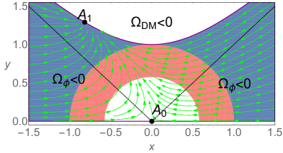
Figure 1: Phase portrait of the dynamical system (12). $A_{0}$ and $A_{1}$ denote the DM-dominated and DE-dominated critical points, respectively. In color/shaded highlighted regions, the universe’s expansion is accelerated, with $w_{tot}<-1$ (blue color, dark shading) and $-1<w_{tot}<-1/3$ (red color, light shading). Orbits starting near $A_{0}$ and converging to $A_{1}$ correspond to the universe’s transition from a past decelerating matter-dominated phase to the present accelerating phase. The dotted black lines correspond to $y=\pm x$ where the phantom equation-of-state parameter $w_{\phi}$ diverges. In this figure, we have considered $\lambda=2$; for other values of this parameter, one would get similar graphics.

Note, however, that such orbits, coming from an infinitely far region of the phase space, obligatory cross the lines $x=y$ or $x=-y$, where the phantom equation-of-state parameter (15) diverges. Therefore, we shall attribute physical meaning to the solution only after the occurrence of this singularity, implying that the phantom DE model should be viewed as a phenomenological model describing the late-time evolution of the universe Bahamonde et al. (2018).

To conclude this section, let us point out that the phase space of the dynamical system (12) can be compactified (see, for instance, Ref. Bahamonde et al. (2018)). However, because of the circumstances described in the previous paragraph, such a procedure is not needed to fully understand the behavior of the orbits of cosmological relevance.

III Coupled phantom dark energy motivated by warm inflation

Let us now turn to the coupled phantom DE cosmological model. The cosmological scenarios in which a phantom DE scalar field directly interacts with the DM component generalize the uncoupled phantom DE model presented in section II. The interaction function characterizing the energy transfer between the phantom DE and DM plays the key role in this context. Given that there is currently no fundamental theory that specifies the exact form of the interaction function between DE and DM, one must resort to a phenomenological approach, considering different couplings with different physical motivations. In this work, we shall consider an interaction function motivated by the warm inflationary scenario. Other choices of the interaction function have been considered in Refs. Fu et al. (2008); Chen et al. (2009).

For the coupled phantom DE cosmological model, the evolution equations are the same as for the uncoupled case of section II, with the exception that Eqs. (7) and (8) now become

$$\ddot{\phi}+3H\dot{\phi}-\frac{\partial V}{\partial\phi} =-\frac{Q}{\dot{\phi}},$$ (19)

$$\dot{\rho}_{\rm DM}+3H\rho_{\rm DM} =-Q.$$ (20)

where $Q$ is the interaction term between the phantom DE scalar field and the DM fluid, determining the energy flow between them. For $Q>0$, the energy flows from DM to phantom DE, while $Q<0$ indicates an energy flow in the opposite direction, i.e., from the phantom scalar field to the DM fluid.

As in section II, we assume the phantom scalar field to have the exponential potential given by Eq. (4).

Inspired by warm inflation, we choose the coupling between DE and DM to be of the form Sá (2023)

$$Q=\Gamma\dot{\phi}^{2},$$ (21)

where $\Gamma$ is a nonzero constant having the dimension of the Hubble rate.

Let us now write the evolution equations, Eqs. (5), (6), (19), and (20) for the coupled phantom DE cosmological model as a dynamical system. Since the interaction term $Q$ cannot be written as a function of the dimensionless variables of $x$ and $y$, introduced in Eq. (10), one extra variable $z$ is needed to close the dynamical system, which, therefore, becomes three dimensional. We choose this extra variable to be Sá (2023)

$$z=\frac{H_{*}}{H\Omega_{\rm DM}+H_{*}},$$ (22)

where $\Omega_{\rm DM}$ is the DM density parameter and $H_{*}$ is a positive constant representing the Hubble parameter at some particular instant $t=t_{*}$.

This choice of $z$ compactifies the phase space in the $z$ direction, between $z=0$ (for $H=+\infty$) and $z=1$ (for $H=0$), but it also introduces a singular term on the evolution equation for $x$, namely, the interaction term becomes proportional to $(1-z)^{-1}$, which diverges for $z\rightarrow 1$. To remove this singularity, we choose a new time variable $\tau$ as Sá (2023)

$$\frac{d\tau}{dt}=\frac{H}{1-z}.$$ (23)

Note that, due to the factor $1-z$, the variable $\tau$ does not have a simple physical interpretation as in the uncoupled case, where, recall, the variable $\eta$, given by Eq. (11) was simply the $e$-fold number.

In the variables $x$, $y$, $z$, and $\tau$, the evolution equations (5), (6), (19), and (20) for the coupled phantom DE cosmological model give rise to the three-dimensional dynamical system

$$x_{\tau} =\left[-\frac{\sqrt{6}}{2}\lambda y^{2}-\frac{3}{2}x(1+x^{2}+y^{2})\right](1-z)$$

$$\hskip 8.53581pt-\alpha x(1+x^{2}-y^{2})z,$$ (24a)

$$y_{\tau} =\left[-\frac{\sqrt{6}}{2}\lambda x+\frac{3}{2}(1-x^{2}-y^{2})\right]y(1-z),$$ (24b)

$$z_{\tau} =\left[\frac{3}{2}(1+x^{2}+y^{2})(1-z)+2\alpha x^{2}z\right]z(1-z),$$ (24c)

where the subscript $\tau$ denotes a derivative with respect to this variable and $\alpha=\Gamma/H_{*}$ is the dimensionless coupling parameter, taken to be nonzero. Following the convention of the direction of the energy transfer between the dark sectors as described above, $\alpha>0$ indicates the energy transfer from the DM sector to the phantom scalar field and $\alpha<0$ corresponds to the energy transfer in the reverse direction.

Note that the above dynamical system is invariant under the transformation $x\rightarrow-x$ and $\lambda\rightarrow-\lambda$, allowing us to assume, without any loss of generality, that the parameter $\lambda$ is positive. Therefore, the parameter space of our coupled phantom DE model is $\{(\alpha,\lambda):\alpha\neq 0,\lambda>0\}$.

In what concerns the DM density parameter $\Omega_{\rm DM}$, the DE density parameter $\Omega_{\phi}$, the phantom equation-of-state parameter $w_{\phi}$, and the total equation-of-state parameter $w_{\rm tot}$, they do not depend on the variable $z$ and, therefore, are given by the same expressions as in the uncoupled case, namely, by Eqs. (13), (14), (15), and (16), respectively.

Inspection of the dynamical system (24) and the evolution equation for the DM density parameter,

$$\Omega_{{\rm DM},\tau}=\Omega_{\rm DM}\left[-3(x^{2}+y^{2})(1-z)-2\alpha x^{2}z\right],$$ (25)

shows that the surfaces $y=0$, $z=0$, $z=1$, and $y=\pm\sqrt{1+x^{2}}$ are invariant manifolds. Since we are not interested in contracting cosmologies (for which $H<0$, implying $y<0$) and taking into account that $\Omega_{\rm DM}\geq 0$, the phase space of the dynamical system should be restricted to the region

$$R_{3}=\left\{(x,y,z)\in\mathbb{R}^{3}:y\leq\sqrt{1+x^{2}},y\geq 0,0\leq z\leq 1\right\}.$$ (26)

This region, however, contains the surfaces $x=\pm y$, at which $w_{\phi}$ diverges, and, furthermore, for $y^{2}<x^{2}$ the DE density parameter $\Omega_{\phi}$ becomes negative. To avoid these unphysical situations, we should further restrict the phase space to the region

$$\overline{R}_{3}=\Bigl{\{}(x,y,z)\in\mathbb{R}^{3}:y\leq\sqrt{1+x^{2}},y^{2}\geq x^{2},$$

$$y\geq 0,0\leq z\leq 1\Bigr{\}},$$ (27)

meaning that our model is only suitable to describe the late-time evolution of the universe, that is, the part of the evolution occurring after the orbits cross the surfaces $x=y$ or $x=-y$. This is the same restriction we have already encountered in the uncoupled scenario (see discussion in section II).

In the finite region of the phase space, the dynamical system (24) has three critical points, $A$, $B$, and $C$, and two critical lines, $D$ and $E$. The qualitative features and the eigenvalues of these critical points are displayed in Table 2 and Table 3, respectively.

Critical point/line	Existence	$\Omega_{\phi}$	$\Omega_{\rm DM}$	$w_{\rm tot}$	Acceleration
$A(0,0,0)$	Always	0	1	0	Never
$B\left(-\frac{\lambda}{\sqrt{6}},\sqrt{1+\frac{\lambda^{2}}{6}},0\right)$	Always	1	0	$-1-\frac{\lambda^{2}}{3}$	Always
$C\left(-\frac{\lambda}{\sqrt{6}},\sqrt{1+\frac{\lambda^{2}}{6}},\frac{3(6+\lambda^{2})}{3(6+\lambda^{2})-2\alpha\lambda^{2}}\right)$	$\alpha<0$	1	0	$-1-\frac{\lambda^{2}}{3}$	Always
$D(0,y,1)$	$0\leq y\leq 1$	$y^{2}$	$1-y^{2}$	$-y^{2}$	$\frac{1}{\sqrt{3}}<y\leq 1$
$E\left(x,\sqrt{1+x^{2}},1\right)$	Always	1	0	$-1-2x^{2}$	Always

Table 2: Properties of the critical points and critical lines of the dynamical system (24) for the coupled phantom DE cosmological model.

Critical point/line	Eigenvalues	Stability
$A(0,0,0)$	$\left(-\frac{3}{2},\frac{3}{2},\frac{3}{2}\right)$	Saddle ($\alpha\neq 0$)
$B\left(-\frac{\lambda}{\sqrt{6}},\sqrt{1+\frac{\lambda^{2}}{6}},0\right)$	$\left(-3-\lambda^{2},-3-\frac{\lambda^{2}}{2},3+\frac{\lambda^{2}}{2}\right)$	Saddle ($\alpha\neq 0$)
$C\left(-\frac{\lambda}{\sqrt{6}},\sqrt{1+\frac{\lambda^{2}}{6}},\frac{3(6+\lambda^{2})}{3(6+\lambda^{2})-2\alpha\lambda^{2}}\right)$	$\left(\frac{\alpha\lambda^{4}}{3\left(6+\lambda^{2}\right)-2\alpha\lambda^{2}},\frac{\alpha\lambda^{2}\left(6+\lambda^{2}\right)}{3\left(6+\lambda^{2}\right)-2\alpha\lambda^{2}},\frac{\alpha\lambda^{2}\left(6+\lambda^{2}\right)}{3\left(6+\lambda^{2}\right)-2\alpha\lambda^{2}}\right)$	Attractor $(\alpha<0)$
$D(0,y,1)$	$\left(0,0,-\alpha\left(1-y^{2}\right)\right)$	Attractor ($\alpha>0$, $y=1$), Saddle (otherwise)
$E\left(x,\sqrt{1+x^{2}},1\right)$	$\left(0,-2\alpha x^{2},-2\alpha x^{2}\right)$	Attractor ($\alpha>0$, $\forall x$)

Table 3: Stability of the critical points and critical lines of the dynamical system (24) for the coupled phantom DE cosmological model.

The critical points $A$ and $B$ were already present in the uncoupled case. However, point $B$ is not anymore an attractor, but rather a saddle point. The critical point $C$, as well as the critical lines $D$ and $E$, are new, arising due to the introduction of a direct coupling between the phantom DE scalar field and the DM fluid.

The critical point $A$ always exists for all allowed values of the model parameters $\alpha$ and $\lambda$. It corresponds to a matter-dominated decelerating solution ($\Omega_{\rm DM}=1$ and $w_{\rm tot}=0$). Since one eigenvalue of the Jacobian matrix of the dynamical system (24) is negative and the other two are positive, linear stability theory indicates that $A$ is unstable, more specifically, it is a saddle point.

The critical point $B$ is also always present, representing a DE-dominated accelerating solution ($\Omega_{\phi}=1$, $w_{\rm tot}<-1$). Because two eigenvalues are negative and one positive, $B$ is also a saddle point: all orbits approaching it near the $\{x,y\}$ plane are repelled along the $z$ direction.

The critical point $C$ belongs to the phase space only if $\alpha<0$, i.e., only when there is an energy transfer from the phantom DE scalar field to the DM fluid. This critical point represents a DE-dominated accelerating solution ($\Omega_{\phi}=1$, $w_{\rm tot}<-1$). Because all eigenvalues are negative, point $C$, whenever exists, is a global attractor to which all orbits converge asymptotically (see Fig. 2).

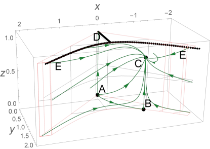
Figure 2: Phase portrait of the dynamical system (24) for $\alpha=-1$ and $\lambda=2$. For negative values of the parameter $\alpha$, the global attractor is the critical point $C$, representing a phantom accelerating solution for which $w_{\rm tot}<-1$.

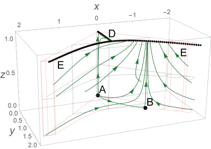
Figure 3: Phase portrait of the dynamical system (24) for $\alpha=1$ and $\lambda=2$. For positive values of the parameter $\alpha$, the attractor is the critical line $E$, representing a phantom accelerating solution for which $w_{\rm tot}<-1$.

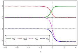
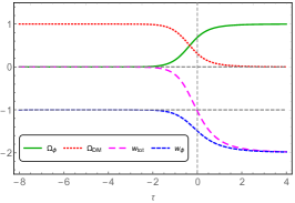
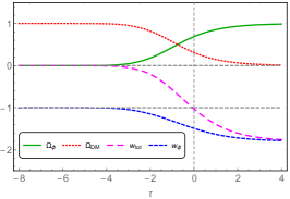
Figure 4: Evolution of $\Omega_{\phi}$, $\Omega_{\rm DM}$, $w_{\phi}$, and $w_{\rm tot}$ for $\alpha=1$ and different values of $\lambda=1.88$, $2.08$, and $2.95$ (left to right panels). Initial conditions at $\tau=-8$ (redshift of about $3000$) are such that all solutions yield $\Omega_{\phi}(0)\approx 0.69$ and $w_{\rm tot}(0)\approx-1.03$. In all cases, the matter-dominated era is long enough to allow for structure formation. Contrarily to the uncoupled scenario, the smaller the parameter $\lambda$, the more phantom the solution is.

The critical line $D$, consisting of a continuous set of critical points, exists for all values of the parameters $\alpha$ and $\lambda$. Critical points with $0<y<1$ correspond to scaling solutions for which the ratio $\Omega_{\rm DM}/\Omega_{\phi}$ is nonzero. Furthermore, these scaling solutions are accelerated if $y>1/\sqrt{3}$. However, as shown in the Appendix using the center manifold theory, these critical points are unstable for $0\leq y<1$ (and any value of $\alpha$), i.e., they cannot correspond to a final state for which $\Omega_{\rm DM}/\Omega_{\phi}\neq 0$ and, therefore, unfortunately, they cannot solve the cosmic coincidence problem. On the other hand, the critical point with $y=1$ is an attractor (for $\alpha>0$), but does not correspond anymore to a scaling solution, since for it the DM density parameter vanishes.

Finally, the non-isolated critical points of the line $E$, which exist for all values of the parameters $\alpha$ and $\lambda$, correspond to DE-dominated accelerating solutions ($\Omega_{\phi}=1$, $w_{\rm tot}<-1$). As shown in the Appendix, these critical points are stable for positive $\alpha$, i.e., for such values of $\alpha$, all orbits converge asymptotically to these points (see Fig. 3).

Among all possible phase-space orbits, only a set reproduces the succession of cosmological eras observed in the late-time evolution of the universe, namely, an era dominated by matter, long enough to allow for structure formation, followed by an era of accelerated expansion.

Let us focus our attention on these cosmologically relevant orbits. They must pass close to the critical point $A$ to guarantee the existence of a long enough matter-dominated era and then proceed to the final state, which is the critical point $C$ if $\alpha<0$ or the critical line $E$ if $\alpha>0$ (see Figs. 2 and 3).

For $\alpha<0$, the final state $C$ has the same $x$ and $y$ coordinates as the global attractor $A_{1}$ of the uncoupled case (see section II), implying that the asymptotic values of the quantities $\Omega_{\phi}$, $\Omega_{\rm DM}$, $w_{\phi}$, and $w_{tot}$, which, recall, depend only on $x$ and $y$, coincide in both cases. Therefore, the introduction of the interaction term (21) between DE and DM does not seem to influence the late-time evolution of the universe if $\Gamma<0$ ($\alpha<0$).

Quite different is the situation for $\alpha>0$. Here, the $x$ and $y$ coordinates of the final state $E$ may not coincide with the corresponding coordinates of the global attractor of the uncoupled case, leading to different late-time behaviors of $\Omega_{\phi}$, $\Omega_{\rm DM}$, $w_{\phi}$, and $w_{tot}$. More specifically, orbits that, after passing near $A$, proceed first to the vicinity of $B$ and only then head to the final state at the critical line $E$, correspond to cosmological solutions similar to those obtained in the uncoupled case. On the contrary, orbits that, after passing near $A$, proceed directly to the final state, end up on a critical point not lying above $B$, and consequently yield different late-time behaviors for the above-referred physical quantities. These two types of orbits can be easily identified in Fig. 3.

Let us analyze in more detail the late-time behavior of $\Omega_{\phi}$, $\Omega_{\rm DM}$, $w_{\phi}$, and $w_{\rm tot}$ for $\alpha>0$, considering three examples for which $\alpha=1$ and $\lambda=1.88$, $2.08$, and $2.95$ (see Fig. 4). In all cases, we choose initial conditions at $\tau=-8$ such that all solutions yield $\Omega_{\phi}(0)\approx 0.69$ and $w_{\rm tot}(0)\approx-1.03$, in agreement with observations.

For $\lambda=1.88$, the corresponding phase-space orbit passes very close to $B$, implying that the $x$ coordinate at the final state is $x_{f}\approx-0.76$, almost the same value as the $x$ coordinate of the critical point $B$, $x_{B}\approx-0.77$. Therefore, the total equation-of-state parameter has similar asymptotic values in the coupled and uncoupled cases, namely, $w_{\rm tot}\approx-2.16$ and $-2.18$, respectively.

For $\lambda=2.08$, the orbit does not pass near $B$, heading directly to a final state with an $x$ coordinate, $x_{f}\approx-0.70$, quite different from the $x$ coordinate of the critical point $B$, $x_{B}\approx-0.85$. This circumstance implies that the asymptotic value of the total equation-of-state parameter, $w_{\rm tot}\approx-1.98$, becomes noticeably higher than the corresponding value in the uncoupled case, $w_{\rm tot}\approx-2.44$. In other words, a direct energy transfer from DM to phantom DE results in a solution less phantom.

This difference between the coupled and uncoupled cases is more pronounced in the case $\lambda=2.95$, in which the corresponding phase-space orbit heads even more directly to the final state, yielding $x_{f}\approx-0.62$ and $w_{\rm tot}\approx-1.77$, while in the uncoupled case these values are $x_{B}\approx-1.20$ and $w_{\rm tot}\approx-3.90$.

The above results can be summarized as follows. In the uncoupled phantom model, the equation-of-state parameter’s asymptotic value is determined solely by $\lambda$, namely, $w_{\rm tot}=-1-\lambda^{2}/3$ (see Table 1). Thus, as $\lambda$ increases, $w_{\rm tot}$ becomes more negative, leading to a solution more phantom. When the direct coupling (21) with $\Gamma>0$ ($\alpha>0$) is introduced in the evolution equations, the equation-of-state parameter depends not only on $\lambda$ but also on the energy exchange between DE and DM. As a result, the asymptotic behavior of $w_{\rm tot}$ is reversed when compared to the uncoupled case, namely, $w_{\rm tot}$ increases with increasing $\lambda$, making the solution less phantom.

To conclude this section, let us point out that outside the phase space $\overline{R}_{3}$, on the boundary of the region $R_{3}$, defined in Eq. (26), for $\alpha<0$, there are two more critical points, namely, $F_{\pm}(\pm 1,0,3/(3-2\alpha))$. Such critical points attract a set of orbits, which, instead of converging to the phantom final state $C$, end up in the unphysical region $y<\pm x$. Such a circumstance would require, in general, the imposition of an additional constraint, either on the phase space or on the parameter space. However, as we have checked numerically, none of the orbits of cosmological relevance (those that guarantee a long enough matter-dominated era by passing near the critical point $A$) is attracted to these unphysical critical points, so we can safely ignore them.

IV Conclusions

Cosmological models with an energy exchange between DE and DM have gathered noteworthy attention in the scientific community because of their rich phenomenological consequences. It is essential to note that the dynamics of such coupled cosmological models depend significantly on the nature of the dark components and the energy exchange rate between them; since none of these features is currently known, there is a large freedom in constructing coupled quintessence and phantom cosmological models.

In this article, we have considered an interacting scenario between a pressureless DM fluid and a phantom DE scalar field with an exponential potential in which the interaction function is motivated by the warm inflationary paradigm. More specifically, we have assumed the interaction term $Q$ to be of the dissipative type, $Q=\Gamma\dot{\phi}^{2}$, where $\Gamma$ is a dissipation coefficient determined by local properties of the dark-sector interactions. In a first, simplified approach to this model, we have chosen $\Gamma$ to be constant, leaving more general cases for future work.

To understand the salient features of the interacting dynamics, we have first reviewed the dynamics of the uncoupled phantom DE cosmological model. Using methods of qualitative analysis of dynamical systems, we have shown that this uncoupled model admits a set of cosmologically relevant solutions that reproduce the succession of cosmological eras observed in the late-time evolution of the universe, namely, an era dominated by matter, long enough to allow for structure formation, followed by the current era of accelerated expansion. However, contrarily to the corresponding uncoupled quintessence model Copeland et al. (1998), there are no scaling attractor solutions; the unique late-time attractor in the uncoupled phantom model describes a Universe completely dominated by phantom DE. Note also that the asymptotic value of the total equation-of-state parameter $w_{\rm tot}=-1-\lambda^{2}/3$ is fixed solely by the choice of the parameter $\lambda$, related to the steepness of the potential of the scalar field.

When the aforementioned direct coupling between the phantom DE scalar field and the DM fluid is introduced in the evolution equations, the dynamical system’s phase space structure changes considerably from what we observe in the uncoupled scenario, allowing for a different late-time behavior of the solutions.

First, the dynamical system of the coupled model admits a set of non-isolated critical points corresponding to accelerated scaling solutions, i.e., solutions for which $\Omega_{\rm DM}/\Omega_{\phi}\neq 0$ and $w_{\rm tot}<-1/3$ (see Table 2). However, since these critical points are unstable for any value of $\alpha$, they do not correspond to a final state of the universe’s evolution and hence the coincidence problem cannot be solved within this particular model.

Second, for $\alpha>0$ (indicating an energy transfer from DM to phantom DE), the asymptotic value of the total equation-of-state parameter $w_{\rm tot}$ is no longer fixed uniquely by the choice of $\lambda$, as in the uncoupled scenario. Instead, it also depends on the energy exchange between the dark components. Our dynamical system analysis shows that, in the coupled scenario, the phase-space orbits asymptotically converge to a critical line, ending up at different points of this line. To each of these points corresponds a different asymptotic value of $w_{\rm tot}$, namely, $w_{\rm tot}=-1-2x_{f}^{2}$, where $x_{f}$ is the $x$ coordinate of the point. The asymptotic values of $w_{\rm tot}$ are such that higher values of $\lambda$ correspond to solutions less phantom, which is exactly the opposite of what happens in the uncoupled scenario. Therefore, a direct energy transfer from DM to DE through a dissipative term inspired by warm inflation significantly alters the late-time behavior of the phantom DE cosmological model.

Based on the outcomes of the present work, we deem it important to further explore the coupled phantom DE cosmological model inspired by warm inflation. In particular, the model with a dissipation coefficient $\Gamma$ depending on both the phantom scalar field and the dark-matter energy density will be considered in future work.

*

Appendix A Stability of the critical lines $D$ and $E$

In this appendix, we investigate the stability of the critical lines $D(0,y,1)$ and $E(x,\sqrt{1+x^{2}},1)$.

Let us start with the critical line $E(x,\sqrt{1+x^{2}},1)$, considering, to that end, a specific point $E(x_{c},\sqrt{1+x_{c}^{2}},1)$, where $-\infty<x_{c}<+\infty$.

The Jacobian matrix of the dynamical system (24), given by

$$J_{E}=\begin{pmatrix}-2\alpha x_{c}^{2}&2\alpha x_{c}\sqrt{1+x_{c}^{2}}&3(1+x_{c}^{2})(x_{c}+\frac{\sqrt{6}}{6}\lambda)\\ 0&0&3x_{c}\sqrt{1+x_{c}^{2}}(x_{c}+\frac{\sqrt{6}}{6}\lambda)\\ 0&0&-2\alpha x_{c}^{2}\end{pmatrix},$$ (28)

has the eigenvalues

$$\lambda_{1}=0,\quad\lambda_{2,3}=-2\alpha x_{c}^{2}.$$ (29)

Since the above Jacobian matrix has only a zero eigenvalue, the non-isolated critical point $E(x_{c},\sqrt{1+x_{c}^{2}},1)$ is normally hyperbolic, meaning that stability can be assessed within the linear theory. Because the nonzero eigenvalues are negative for $\alpha>0$, this critical point is an attractor for such values of the parameter $\alpha$.

Let us now turn to the analysis of the stability of the critical line $D(0,y,1)$, considering, to that end, a specific point $D(0,y_{c},1)$, where $0\leq y_{c}<1$.

The Jacobian matrix of the dynamical system (24), given by

$$J_{D}=\begin{pmatrix}\alpha(y_{c}^{2}-1)&0&\frac{\sqrt{6}}{2}\lambda y_{c}^{2}\\ 0&0&\frac{3}{2}y_{c}(y_{c}^{2}-1)\\ 0&0&0\end{pmatrix},$$ (30)

has the eigenvalues

$$\lambda_{1}=\alpha(y_{c}^{2}-1),\quad\lambda_{2,3}=0,$$ (31)

to which correspond the (generalized) eigenvectors

$$v_{1}=\begin{pmatrix}1\\ 0\\ 0\end{pmatrix},\quad v_{2}=\begin{pmatrix}0\\ 1\\ 0\end{pmatrix},\quad v_{3}=\begin{pmatrix}\frac{\sqrt{6}\lambda y_{c}^{2}}{2\alpha(1-y_{c}^{2})}\\ 0\\ 1\end{pmatrix}.$$ (32)

Since the Jacobian matrix $J_{D}$ has two zero eigenvalues, the linear theory is not enough to assess the stability of the critical point $D(0,y_{c},1)$ and, consequently, one has to resort to alternative methods. Here, we choose the center manifold theory Carr (1982); Guckenheimer and Holmes (1983); Bogoyavlensky (1985).

To shift the critical point $D(0,y_{c},1)$ to the origin of the coordinate system, we introduce new variables

$$u=x,\quad v=y-y_{c},\quad w=z-1,$$ (33)

for which the dynamical system (24) becomes

$$u_{\tau} =-\alpha(1-y_{c}^{2})u+\frac{\sqrt{6}}{2}\lambda y_{c}^{2}w+f_{1}(u,v,w),$$ (34a)

$$v_{\tau} =-\frac{3}{2}y_{c}(1-y_{c}^{2})w+f_{2}(u,v,w),$$ (34b)

$$w_{\tau} =f_{3}(u,v,w),$$ (34c)

where $f_{i}=\mathcal{O}(u^{2},v^{2},w^{2},uv,uw,vw)$, $i=1,2,3$.

Another change of variables, namely,

$$\begin{pmatrix}u\\ v\\ w\end{pmatrix}=S\begin{pmatrix}U\\ V\\ W\end{pmatrix},$$ (35)

where $S$ is a matrix whose columns are the generalized eigenvectors (32), brings the dynamical system to the form

$$U_{\tau} =-\alpha(1-y_{c}^{2})U+F_{1}(U,V,W),$$ (36a)

$$V_{\tau} =-\frac{3}{2}y_{c}(1-y_{c}^{2})W+F_{2}(U,V,W),$$ (36b)

$$W_{\tau} =F_{3}(U,V,W),$$ (36c)

where $F_{i}=\mathcal{O}(U^{2},V^{2},W^{2},UV,UW,VW)$, $i=1,2,3$.

Before proceeding to the determination of the center manifold $U=h(V,W)$ and the flow on it, let us point out that along the $U$ direction, the orbits approach the critical point for $\alpha>0$ and move away from it for $\alpha<0$.

Now, the center manifold is a solution to the partial differential equation

$$\frac{\partial h}{\partial V}\left[-\frac{3}{2}y_{c}(1-y_{c}^{2})W+F_{2}\Big{(}h(V,W),V,W\Big{)}\right]$$

$$\hskip 14.22636pt+\frac{\partial h}{\partial W}F_{3}\Big{(}h(V,W),V,W\Big{)}+\alpha(1-y_{c}^{2})h(V,W)$$

$$\hskip 14.22636pt-F_{1}\Big{(}h(V,W),V,W\Big{)}=0,$$ (37)

where $h(V,W)$ is defined on some neighborhood of the critical point with $h(0,0)$ and $\nabla h(0,0)=0$.

Searching for a solution to the above equation of the form

$$h(V,W)=\sum_{j=2}^{m}\sum_{i=0}^{j}a_{i,j-i}V^{i}W^{j-i},$$ (38)

where $a_{ij}$ are constants and $m\geq 2$, we obtain, at lowest order in powers of $V$ and $W$,

$$U=\frac{\sqrt{6}\lambda y_{c}}{\alpha(1-y_{c}^{2})^{2}}VW+\frac{\sqrt{6}\lambda y_{c}^{2}[3-\alpha(1-y_{c}^{2})]}{2\alpha^{2}(1-y_{c}^{2})^{2}}W^{2}.$$ (39)

As both terms of the above solution vanish for $y_{c}=0$, for such a value of $y_{c}$ we have to extend our calculation to the third order in powers of V and W, obtaining

$$U=\frac{\sqrt{6}\lambda}{2\alpha}V^{2}W.$$ (40)

The flow on the center manifold is determined by the differential equations

$$V_{\tau} =-\frac{3}{2}y_{c}(1-y_{c}^{2})W,$$ (41a)

$$W_{\tau} =\frac{3}{2}(1+y_{c}^{2})W^{2}.$$ (41b)

Again, the right-hand side of Eq. (41a) vanishes for $y_{c}=0$, requiring, for such a value of $y_{c}$, to extend the calculation to higher orders in powers of $V$ and $W$. The flow on the center manifold is then, for $y_{c}=0$, determined by the differential equations

$$V_{\tau} =-\frac{3}{2}VW,$$ (42a)

$$W_{\tau} =\frac{3}{2}W^{2}.$$ (42b)

For $0<y_{c}<1$, taking into account that $W<0$ in the neighborhood of the critical point, it follows that both $V_{\tau}$ and $W_{\tau}$ are positive and, consequently, the orbits approach the critical point along the $W$-direction and drift in the direction of increasing $V$. For the case $y_{c}=0$, taking also into account that $V>0$, we arrive at the very same conclusion. Note that this result does not depend on the parameter $\alpha$, contrarily to the result obtained for the flow along the $U$-direction, which, as mentioned above, approaches the critical point for $\alpha>0$ and moves away from it for $\alpha<0$.

In terms of the original variables $x$, $y$, and $z$, the above results mean that, for $\alpha>0$, the orbits, when approaching the critical line $D(0,y,1)$, drift in the $y$-direction, towards the critical point $D(0,1,1)$, which coincides with the point $E(0,1,1)$ of the critical line $E(x,\sqrt{1+x^{2}},1)$.

This result, together with the stability analysis of the critical line $E(x,\sqrt{1+x^{2}},1)$, leads to the conclusion that for positive values of the parameter $\alpha$ the critical line $E(x,\sqrt{1+x^{2}},1)$ is an attractor, i.e., all orbits (except the heteroclinic ones, connecting critical points along the boundaries of the phase space) asymptotically converge to one of the points of this critical line.

References

- Penzias and Wilson (1965) Arno A. Penzias and Robert Woodrow Wilson, “A Measurement of Excess Antenna Temperature at 4080 Mc/s,” Astrophys. J. 142, 419–421 (1965).
- Guth (1981) Alan H. Guth, “Inflationary universe: A possible solution to the horizon and flatness problems,” Phys. Rev. D 23, 347–356 (1981).
- Linde (1982) Andrei D. Linde, “A new inflationary universe scenario: A possible solution of the horizon, flatness, homogeneity, isotropy and primordial monopole problems,” Phys. Lett. B 108, 389–393 (1982).
- Riess et al. (1998) Adam G. Riess et al. (Supernova Search Team), “Observational Evidence from Supernovae for an Accelerating Universe and a Cosmological Constant,” Astron. J. 116, 1009–1038 (1998), arXiv:astro-ph/9805201 .
- Perlmutter et al. (1999) S. Perlmutter et al. (Supernova Cosmology Project), “Measurements of and from 42 High-Redshift Supernovae,” Astrophys. J. 517, 565–586 (1999), arXiv:astro-ph/9812133 .
- Astier and Pain (2012) Pierre Astier and Reynald Pain, “Observational evidence of the accelerated expansion of the universe,” C. R. Phys. 13, 521–538 (2012), arXiv:1204.5493 [astro-ph.CO] .
- Peebles and Ratra (2003) P. J. E. Peebles and Bharat Ratra, “The cosmological constant and dark energy,” Rev. Mod. Phys. 75, 559–606 (2003), arXiv:astro-ph/0207347 .
- Copeland et al. (2006) Edmund J. Copeland, M. Sami, and Shinji Tsujikawa, “Dynamics of dark energy,” Int. J. Mod. Phys. D 15, 1753–1936 (2006), arXiv:hep-th/0603057 .
- Sahni and Starobinsky (2006) Varun Sahni and Alexei Starobinsky, “Reconstructing dark energy,” Int. J. Mod. Phys. D 15, 2105–2132 (2006), arXiv:astro-ph/0610026 .
- Bamba et al. (2012) Kazuharu Bamba, Salvatore Capozziello, Shin’ichi Nojiri, and Sergei D. Odintsov, “Dark energy cosmology: the equivalent description via different theoretical models and cosmography tests,” Astrophys. Space Sci. 342, 155–228 (2012), arXiv:1205.3421 [gr-qc] .
- Nojiri and Odintsov (2007) Shin’ichi Nojiri and Sergei D. Odintsov, “Introduction to modified gravity and gravitational alternative for dark energy,” Int. J. Geom. Meth. Mod. Phys. 4, 115 (2007), arXiv:hep-th/0601213 .
- Nojiri and Odintsov (2011) Shin’ichi Nojiri and Sergei D. Odintsov, “Unified cosmic history in modified gravity: from theory to Lorentz non-invariant models,” Phys. Rept. 505, 59–144 (2011), arXiv:1011.0544 [gr-qc] .
- De Felice and Tsujikawa (2010) Antonio De Felice and Shinji Tsujikawa, “ Theories,” Living Rev. Rel. 13, 3 (2010), arXiv:1002.4928 [gr-qc] .
- Capozziello and De Laurentis (2011) Salvatore Capozziello and Mariafelicia De Laurentis, “Extended Theories of Gravity,” Phys. Rept. 509, 167–321 (2011), arXiv:1108.6266 [gr-qc] .
- Clifton et al. (2012) Timothy Clifton, Pedro G. Ferreira, Antonio Padilla, and Constantinos Skordis, “Modified gravity and cosmology,” Phys. Rept. 513, 1–189 (2012), arXiv:1106.2476 [astro-ph.CO] .
- Koyama (2016) Kazuya Koyama, “Cosmological tests of modified gravity,” Rept. Prog. Phys. 79, 046902 (2016), arXiv:1504.04623 [astro-ph.CO] .
- Cai et al. (2016) Yi-Fu Cai, Salvatore Capozziello, Mariafelicia De Laurentis, and Emmanuel N. Saridakis, “ teleparallel gravity and cosmology,” Rept. Prog. Phys. 79, 106901 (2016), arXiv:1511.07586 [gr-qc] .
- Nojiri et al. (2017) S. Nojiri, S. D. Odintsov, and V. K. Oikonomou, “Modified gravity theories on a nutshell: Inflation, bounce and late-time evolution,” Phys. Rept. 692, 1–104 (2017), arXiv:1705.11098 [gr-qc] .
- Bahamonde et al. (2023) Sebastian Bahamonde, Konstantinos F. Dialektopoulos, Celia Escamilla-Rivera, Gabriel Farrugia, Viktor Gakis, Martin Hendry, Manuel Hohmann, Jackson Levi Said, Jurgen Mifsud, and Eleonora Di Valentino, “Teleparallel gravity: from theory to cosmology,” Rept. Prog. Phys. 86, 026901 (2023), arXiv:2106.13793 [gr-qc] .
- Weinberg (1989) Steven Weinberg, “The cosmological constant problem,” Rev. Mod. Phys. 61, 1–23 (1989).
- Zlatev et al. (1999) Ivaylo Zlatev, Limin Wang, and Paul J. Steinhardt, “Quintessence, Cosmic Coincidence, and the Cosmological Constant,” Phys. Rev. Lett. 82, 896–899 (1999), arXiv:astro-ph/9807002 .
- Abdalla et al. (2022) Elcio Abdalla et al., “Cosmology intertwined: A review of the particle physics, astrophysics, and cosmology associated with the cosmological tensions and anomalies,” JHEAp 34, 49–211 (2022), arXiv:2203.06142 [astro-ph.CO] .
- Amendola (2000) Luca Amendola, “Coupled quintessence,” Phys. Rev. D 62, 043511 (2000), arXiv:astro-ph/9908023 .
- Cai and Wang (2005) Rong-Gen Cai and Anzhong Wang, “Cosmology with interaction between phantom dark energy and dark matter and the coincidence problem,” JCAP 03, 002 (2005), arXiv:hep-th/0411025 .
- Pavon and Zimdahl (2005) Diego Pavon and Winfried Zimdahl, “Holographic dark energy and cosmic coincidence,” Phys. Lett. B 628, 206–210 (2005), arXiv:gr-qc/0505020 .
- Huey and Wandelt (2006) Greg Huey and Benjamin D. Wandelt, “Interacting quintessence, the coincidence problem, and cosmic acceleration,” Phys. Rev. D 74, 023519 (2006), arXiv:astro-ph/0407196 .
- del Campo et al. (2008) Sergio del Campo, Ramon Herrera, and Diego Pavon, “Toward a solution of the coincidence problem,” Phys. Rev. D 78, 021302 (2008), arXiv:0806.2116 [astro-ph] .
- del Campo et al. (2009) Sergio del Campo, Ramon Herrera, and Diego Pavon, “Interacting models may be key to solve the cosmic coincidence problem,” JCAP 01, 020 (2009), arXiv:0812.2210 [gr-qc] .
- Wang et al. (2005) Bin Wang, Yun-gui Gong, and Elcio Abdalla, “Transition of the dark energy equation of state in an interacting holographic dark energy model,” Phys. Lett. B 624, 141–146 (2005), arXiv:hep-th/0506069 .
- Das et al. (2006) Subinoy Das, Pier Stefano Corasaniti, and Justin Khoury, “Superacceleration as the signature of a dark sector interaction,” Phys. Rev. D 73, 083509 (2006), arXiv:astro-ph/0510628 .
- Sadjadi and Honardoost (2007) H. Mohseni Sadjadi and M. Honardoost, “Thermodynamics second law and crossing(s) in interacting holographic dark energy model,” Phys. Lett. B 647, 231–236 (2007), arXiv:gr-qc/0609076 .
- Pan and Chakraborty (2014) Supriya Pan and Subenoy Chakraborty, “A cosmographic analysis of holographic dark energy models,” Int. J. Mod. Phys. D 23, 1450092 (2014), arXiv:1410.8281 [gr-qc] .
- Kumar and Nunes (2017) Suresh Kumar and Rafael C. Nunes, “Echo of interactions in the dark sector,” Phys. Rev. D 96, 103511 (2017), arXiv:1702.02143 [astro-ph.CO] .
- Di Valentino et al. (2017) Eleonora Di Valentino, Alessandro Melchiorri, and Olga Mena, “Can interacting dark energy solve the tension?” Phys. Rev. D 96, 043503 (2017), arXiv:1704.08342 [astro-ph.CO] .
- Yang et al. (2018a) Weiqiang Yang, Supriya Pan, Eleonora Di Valentino, Rafael C. Nunes, Sunny Vagnozzi, and David F. Mota, “Tale of stable interacting dark energy, observational signatures, and the tension,” JCAP 09, 019 (2018a), arXiv:1805.08252 [astro-ph.CO] .
- Pan et al. (2019) Supriya Pan, Weiqiang Yang, Eleonora Di Valentino, Emmanuel N. Saridakis, and Subenoy Chakraborty, “Interacting scenarios with dynamical dark energy: Observational constraints and alleviation of the tension,” Phys. Rev. D 100, 103520 (2019), arXiv:1907.07540 [astro-ph.CO] .
- Pourtsidou and Tram (2016) Alkistis Pourtsidou and Thomas Tram, “Reconciling CMB and structure growth measurements with dark energy interactions,” Phys. Rev. D 94, 043518 (2016), arXiv:1604.04222 [astro-ph.CO] .
- An et al. (2018) Rui An, Chang Feng, and Bin Wang, “Relieving the tension between weak lensing and cosmic microwave background with interacting dark matter and dark energy models,” JCAP 02, 038 (2018), arXiv:1711.06799 [astro-ph.CO] .
- Kumar et al. (2019) Suresh Kumar, Rafael C. Nunes, and Santosh Kumar Yadav, “Dark sector interaction: a remedy of the tensions between CMB and LSS data,” Eur. Phys. J. C 79, 576 (2019), arXiv:1903.04865 [astro-ph.CO] .
- Barrow and Clifton (2006) John D. Barrow and T. Clifton, “Cosmologies with energy exchange,” Phys. Rev. D 73, 103520 (2006), arXiv:gr-qc/0604063 .
- Valiviita et al. (2008) Jussi Valiviita, Elisabetta Majerotto, and Roy Maartens, “Large-scale instability in interacting dark energy and dark matter fluids,” JCAP 07, 020 (2008), arXiv:0804.0232 [astro-ph] .
- Henriques et al. (2009) Alfredo Barbosa Henriques, Robertus Potting, and Paulo M. Sá, “Unification of inflation, dark energy, and dark matter within the Salam-Sezgin cosmological model,” Phys. Rev. D 79, 103522 (2009), arXiv:0903.2014 [astro-ph.CO] .
- Gavela et al. (2009) M. B. Gavela, D. Hernandez, L. Lopez Honorez, O. Mena, and S. Rigolin, “Dark coupling,” JCAP 07, 034 (2009), [Erratum: JCAP 05, E01 (2010)], arXiv:0901.1611 [astro-ph.CO] .
- Valiviita et al. (2010) Jussi Valiviita, Roy Maartens, and Elisabetta Majerotto, “Observational constraints on an interacting dark energy model,” Mon. Not. Roy. Astron. Soc. 402, 2355–2368 (2010), arXiv:0907.4987 [astro-ph.CO] .
- Cao et al. (2011) Shuo Cao, Nan Liang, and Zong-Hong Zhu, “Testing the phenomenological interacting dark energy with observational data,” Mon. Not. Roy. Astron. Soc. 416, 1099–1104 (2011), arXiv:1012.4879 [astro-ph.CO] .
- He et al. (2011) Jian-Hua He, Bin Wang, and Elcio Abdalla, “Deep connection between gravity and the interacting dark sector model,” Phys. Rev. D 84, 123526 (2011), arXiv:1109.1730 [gr-qc] .
- Yang and Xu (2014a) Weiqiang Yang and Lixin Xu, “Cosmological constraints on interacting dark energy with redshift-space distortion after Planck data,” Phys. Rev. D 89, 083517 (2014a), arXiv:1401.1286 [astro-ph.CO] .
- Li and Zhang (2014) Yun-He Li and Xin Zhang, “Large-scale stable interacting dark energy model: Cosmological perturbations and observational constraints,” Phys. Rev. D 89, 083009 (2014), arXiv:1312.6328 [astro-ph.CO] .
- Yang and Xu (2014b) Weiqiang Yang and Lixin Xu, “Testing coupled dark energy with large scale structure observation,” JCAP 08, 034 (2014b), arXiv:1401.5177 [astro-ph.CO] .
- Yang and Xu (2014c) Weiqiang Yang and Lixin Xu, “Coupled dark energy with perturbed Hubble expansion rate,” Phys. Rev. D 90, 083532 (2014c), arXiv:1409.5533 [astro-ph.CO] .
- Pan et al. (2015) Supriya Pan, Subhra Bhattacharya, and Subenoy Chakraborty, “An analytic model for interacting dark energy and its observational constraints,” Mon. Not. Roy. Astron. Soc. 452, 3038–3046 (2015), arXiv:1210.0396 [gr-qc] .
- Nunes et al. (2016) Rafael C. Nunes, Supriya Pan, and Emmanuel N. Saridakis, “New constraints on interacting dark energy from cosmic chronometers,” Phys. Rev. D 94, 023508 (2016), arXiv:1605.01712 [astro-ph.CO] .
- Yang et al. (2016) Weiqiang Yang, Hang Li, Yabo Wu, and Jianbo Lu, “Cosmological constraints on coupled dark energy,” JCAP 10, 007 (2016), arXiv:1608.07039 [astro-ph.CO] .
- Yang et al. (2017a) Weiqiang Yang, Narayan Banerjee, and Supriya Pan, “Constraining a dark matter and dark energy interaction scenario with a dynamical equation of state,” Phys. Rev. D 95, 123527 (2017a), [Addendum: Phys. Rev. D 96, 089903 (2017)], arXiv:1705.09278 [astro-ph.CO] .
- Yang et al. (2017b) Weiqiang Yang, Lixin Xu, Hang Li, Yabo Wu, and Jianbo Lu, “Testing the Interacting Dark Energy Model with Cosmic Microwave Background Anisotropy and Observational Hubble Data,” Entropy 19, 327 (2017b).
- Mifsud and Van De Bruck (2017) Jurgen Mifsud and Carsten Van De Bruck, “Probing the imprints of generalized interacting dark energy on the growth of perturbations,” JCAP 11, 001 (2017), arXiv:1707.07667 [astro-ph.CO] .
- Yang et al. (2017c) Weiqiang Yang, Supriya Pan, and David F. Mota, “Novel approach toward the large-scale stable interacting dark-energy models and their astronomical bounds,” Phys. Rev. D 96, 123508 (2017c), arXiv:1709.00006 [astro-ph.CO] .
- Yang et al. (2018b) Weiqiang Yang, Supriya Pan, and John D. Barrow, “Large-scale stability and astronomical constraints for coupled dark-energy models,” Phys. Rev. D 97, 043529 (2018b), arXiv:1706.04953 [astro-ph.CO] .
- Yang et al. (2018c) Weiqiang Yang, Ankan Mukherjee, Eleonora Di Valentino, and Supriya Pan, “Interacting dark energy with time varying equation of state and the tension,” Phys. Rev. D 98, 123527 (2018c), arXiv:1809.06883 [astro-ph.CO] .
- Pan et al. (2020a) Supriya Pan, German S. Sharov, and Weiqiang Yang, “Field theoretic interpretations of interacting dark energy scenarios and recent observations,” Phys. Rev. D 101, 103533 (2020a), arXiv:2001.03120 [astro-ph.CO] .
- Sá (2020a) Paulo M. Sá, “Unified Description of Dark Energy and Dark Matter within the Generalized Hybrid Metric-Palatini Theory of Gravity,” Universe 6, 78 (2020a), arXiv:2002.09446 [gr-qc] .
- Pan et al. (2020b) Supriya Pan, Jaume de Haro, Weiqiang Yang, and Jaume Amorós, “Understanding the phenomenology of interacting dark energy scenarios and their theoretical bounds,” Phys. Rev. D 101, 123506 (2020b), arXiv:2001.09885 [gr-qc] .
- Sá (2020b) Paulo M. Sá, “Triple unification of inflation, dark energy, and dark matter in two-scalar-field cosmology,” Phys. Rev. D 102, 103519 (2020b), arXiv:2007.07109 [gr-qc] .
- Di Valentino et al. (2020) Eleonora Di Valentino, Alessandro Melchiorri, Olga Mena, and Sunny Vagnozzi, “Interacting dark energy in the early 2020s: A promising solution to the and cosmic shear tensions,” Phys. Dark Univ. 30, 100666 (2020), arXiv:1908.04281 [astro-ph.CO] .
- Di Valentino et al. (2021) Eleonora Di Valentino, Alessandro Melchiorri, Olga Mena, Supriya Pan, and Weiqiang Yang, “Interacting dark energy in a closed universe,” Mon. Not. Roy. Astron. Soc. 502, L23–L28 (2021), arXiv:2011.00283 [astro-ph.CO] .
- Sá (2021) Paulo M. Sá, “Late-time evolution of the Universe within a two-scalar-field cosmological model,” Phys. Rev. D 103, 123517 (2021), arXiv:2103.01693 [gr-qc] .
- Gao et al. (2021) Li-Yang Gao, Ze-Wei Zhao, She-Sheng Xue, and Xin Zhang, “Relieving the tension with a new interacting dark energy model,” JCAP 07, 005 (2021), arXiv:2101.10714 [astro-ph.CO] .
- Yang et al. (2021) Weiqiang Yang, Supriya Pan, Eleonora Di Valentino, Olga Mena, and Alessandro Melchiorri, “2021- odyssey: closed, phantom and interacting dark energy cosmologies,” JCAP 10, 008 (2021), arXiv:2101.03129 [astro-ph.CO] .
- Lucca (2021) Matteo Lucca, “Multi-interacting dark energy and its cosmological implications,” Phys. Rev. D 104, 083510 (2021), arXiv:2106.15196 [astro-ph.CO] .
- Potting and Sá (2022) Robertus Potting and Paulo M. Sá, “Coupled quintessence with a generalized interaction term,” Int. J. Mod. Phys. D 31, 2250111 (2022), arXiv:2112.07608 [gr-qc] .
- Chatzidakis et al. (2022) S. Chatzidakis, A. Giacomini, P. G. L. Leach, G. Leon, A. Paliathanasis, and Supriya Pan, “Interacting dark energy in curved FLRW spacetime from Weyl Integrable Spacetime,” JHEAp 36, 141–151 (2022), arXiv:2206.06639 [gr-qc] .
- Zhai et al. (2023) Yuejia Zhai, William Giarè, Carsten van de Bruck, Eleonora Di Valentino, Olga Mena, and Rafael C. Nunes, “A consistent view of interacting dark energy from multiple CMB probes,” JCAP 07, 032 (2023), arXiv:2303.08201 [astro-ph.CO] .
- Li and Zhang (2023) Yun-He Li and Xin Zhang, “IDECAMB: an implementation of interacting dark energy cosmology in CAMB,” JCAP 09, 046 (2023), arXiv:2306.01593 [astro-ph.CO] .
- Teixeira et al. (2023) Elsa M. Teixeira, Richard Daniel, Noemi Frusciante, and Carsten van de Bruck, “Forecasts on interacting dark energy with standard sirens,” Phys. Rev. D 108, 084070 (2023), arXiv:2309.06544 [astro-ph.CO] .
- Sá (2023) Paulo M. Sá, “Coupled quintessence inspired by warm inflation,” (2023), arXiv:2312.09171 [gr-qc] .
- Giarè et al. (2024a) William Giarè, Yuejia Zhai, Supriya Pan, Eleonora Di Valentino, Rafael C. Nunes, and Carsten van de Bruck, “Tightening the reins on non-minimal dark sector physics: Interacting Dark Energy with dynamical and non-dynamical equation of state,” (2024a), arXiv:2404.02110 [astro-ph.CO] .
- Halder et al. (2024) Sudip Halder, Jaume de Haro, Tapan Saha, and Supriya Pan, “Phase space analysis of sign-shifting interacting dark energy models,” Phys. Rev. D 109, 083522 (2024), arXiv:2403.01397 [gr-qc] .
- Giarè et al. (2024b) William Giarè, Miguel A. Sabogal, Rafael C. Nunes, and Eleonora Di Valentino, “Interacting Dark Energy after DESI Baryon Acoustic Oscillation measurements,” (2024b), arXiv:2404.15232 [astro-ph.CO] .
- Berera (1995) Arjun Berera, “Warm inflation,” Phys. Rev. Lett. 75, 3218–3221 (1995), arXiv:astro-ph/9509049 .
- Berera (2023) Arjun Berera, “The Warm Inflation Story,” Universe 9, 272 (2023), arXiv:2305.10879 [hep-ph] .
- Caldwell (2002) R. R. Caldwell, “A phantom menace? Cosmological consequences of a dark energy component with super-negative equation of state,” Phys. Lett. B 545, 23–29 (2002), arXiv:astro-ph/9908168 .
- Schulz and White (2001) A. E. Schulz and Martin J. White, “Tensor to scalar ratio of phantom dark energy models,” Phys. Rev. D 64, 043514 (2001), arXiv:astro-ph/0104112 .
- Gibbons (2003) G. W. Gibbons, “Phantom matter and the cosmological constant,” (2003), arXiv:hep-th/0302199 .
- Li and Hao (2004) Xin-zhou Li and Jian-gang Hao, “Phantom field with symmetry in an exponential potential,” Phys. Rev. D 69, 107303 (2004), arXiv:hep-th/0303093 .
- Hao and Li (2004) Jian-Gang Hao and Xin-zhou Li, “Phantom cosmic dynamics: Tracking attractor and cosmic doomsday,” Phys. Rev. D 70, 043529 (2004), arXiv:astro-ph/0309746 .
- Chimento and Lazkoz (2003) Luis P. Chimento and Ruth Lazkoz, “Constructing Phantom Cosmologies from Standard Scalar Field Universes,” Phys. Rev. Lett. 91, 211301 (2003), arXiv:gr-qc/0307111 .
- Vikman (2005) Alexander Vikman, “Can dark energy evolve to the phantom?” Phys. Rev. D 71, 023515 (2005), arXiv:astro-ph/0407107 .
- Ludwick (2017) Kevin J. Ludwick, “The viability of phantom dark energy: A review,” Mod. Phys. Lett. A 32, 1730025 (2017), arXiv:1708.06981 [astro-ph.CO] .
- Carroll et al. (2003) Sean M. Carroll, Mark Hoffman, and Mark Trodden, “Can the dark energy equation-of-state parameter be less than ?” Phys. Rev. D 68, 023509 (2003), arXiv:astro-ph/0301273 .
- Bahamonde et al. (2018) Sebastian Bahamonde, Christian G. Böhmer, Sante Carloni, Edmund J. Copeland, Wei Fang, and Nicola Tamanini, “Dynamical systems applied to cosmology: Dark energy and modified gravity,” Phys. Rept. 775-777, 1–122 (2018), arXiv:1712.03107 [gr-qc] .
- Fu et al. (2008) Xiangyun Fu, Hong Wei Yu, and Puxun Wu, “Dynamics of interacting phantom scalar field dark energy in loop quantum cosmology,” Phys. Rev. D 78, 063001 (2008), arXiv:0808.1382 [gr-qc] .
- Chen et al. (2009) Xi-ming Chen, Yun-gui Gong, and Emmanuel N. Saridakis, “Phase-space analysis of interacting phantom cosmology,” JCAP 04, 001 (2009), arXiv:0812.1117 [gr-qc] .
- Copeland et al. (1998) E. J. Copeland, A. R. Liddle, and D Wands, “Exponential potentials and cosmological scaling solutions,” Phys. Rev. D 57, 4686–4690 (1998), arXiv:gr-qc/9711068 .
- Carr (1982) Jack Carr, Applications of Centre Manifold Theory (Springer, New York, 1982).
- Guckenheimer and Holmes (1983) John Guckenheimer and Philip Holmes, Nonlinear Oscillations, Dynamical Systems, and Bifurcations of Vector Fields (Springer, New York, 1983).
- Bogoyavlensky (1985) Oleg I. Bogoyavlensky, Methods in the Qualitative Theory of Dynamical Systems in Astrophysics and Gas Dynamics (Springer-Verlag, Berlin, Heidelberg, 1985).