Online closed testing with e-values

Abstract

In contemporary research, data scientists often test an infinite sequence of hypotheses $H_{1},H_{2},\ldots$ one by one, and are required to make real-time decisions without knowing the future hypotheses or data. In this paper, we consider such an online multiple testing problem with the goal of providing simultaneous lower bounds for the number of true discoveries in data-adaptively chosen rejection sets. Using the (online) closure principle, we show that for this task it is necessary to use an anytime-valid test for each intersection hypothesis. Motivated by this result, we construct a new online closed testing procedure and a corresponding short-cut with a true discovery guarantee based on multiplying sequential e-values. This general but simple procedure gives uniform improvements over existing methods but also allows to construct entirely new and powerful procedures. In addition, we introduce new ideas for hedging and boosting of sequential e-values that provably increase power. Finally, we also propose the first online true discovery procedure for arbitrarily dependent e-values.

1 Introduction

Online multiple testing is a framework in which a potentially infinite stream of hypotheses $H_{1},H_{2},\ldots$ is tested one by one over time [10, 20]. At each step $t\in\mathbb{N}$ it needs to be decided on the current hypothesis $H_{t}$ without knowing how many hypotheses are to be tested in the future, what those hypotheses are, and without having access to all the data relevant to testing them (indeed, that data may only be collected in the future). This setting occurs in the tech industry [23, 28], machine learning [8, 49], open data repositories as used in genomics [1, 27, 5] and other data science tasks where flexible and real-time decision making is required.

A common error metric for a chosen rejection set $R_{t}$ at time $t$ is the false discovery proportion

$$\mathrm{FDP}(R_{t})=\frac{\text{Number of true hypotheses in }R_{t}}{\text{Size of }R_{t}}.$$ (1)

The usual approach, both in online and classical offline testing, is to control the expected value of $\mathrm{FDP}(R_{t})$, also known as the false discovery rate (FDR) [2], below some level $\alpha\in(0,1)$. However, since the $\mathrm{FDP}$ may have high variance, controlling its expectation may not be enough.

In a seminal work, Goeman and Solari [14] proposed to control the tail probabilities of $\mathrm{FDP}(S)$ simultaneously over all possible rejection sets $S$ instead. That means they suggest to provide an upper bound $\boldsymbol{q}(S)$ for $\mathrm{FDP}(S)$ such that the probability that there is any set $S$ with $\boldsymbol{q}(S)<\mathrm{FDP}(S)$, is less or equal than $\alpha$. The advantage compared to FDR control is that the rejection set can be chosen post-hoc, meaning after looking at the data and calculating the bounds $\boldsymbol{q}(S)$, without violating this error control. Their work focused on offline multiple testing, while we study this error metric in the online setting.

For the online setting the above simultaneity has the additional benefit that the testing process can be stopped data-adaptively at any time, while online FDR control is usually only provided at fixed times [50, 47]. This guarantee at stopping times yields a much higher flexibility which is highly valuable in the online setting.

Another obvious difference to FDR control is that we obtain a bound that holds with high probability instead of controlling the expectation which can be advantageous in applications where an inflated false discovery proportion has severe consequences. However, there are also connections between FDR and simultaneous FDP controlling procedures as illustrated by Goeman et al. [15] with the example of the Benjamini-Hochberg procedure [2] and by Katsevich and Ramdas [21] for several other problems. As done by Goeman et al. [16], we will consider simultaneous lower bounds on the true discovery proportion in this paper, which is mathematically equivalent to upper bounding the false discovery proportion, but easier to handle.

A recently popularized approach for online testing of a single hypothesis, where not the hypotheses but the data itself comes in sequentially, is the e-value. An e-value $E_{t}$ for a hypothesis $H_{t}$ is a nonnegative random variable which has expected value less or equal than one if $H_{t}$ is true. The e-value is an alternative to the well-known p-value but more suitable for settings where early stopping of the sampling process or optional continuation is desired [34, 17, 30]. In this paper, we exploit this sequential suitability of the e-value to design online multiple testing procedures with simultaneous true discovery guarantees.

1.1 Related literature

Our work mixes ingredients from different subfields of sequential and multiple hypothesis testing.

The e-value has recently emerged as a fundamental concept in composite hypothesis testing and underlying a universal approach to anytime-valid inference [45, 33, 39, 17, 29], but the concept can be traced back to the works of Ville [38], Wald [43], Darling and Robbins [6]. A recent overview of the e-value literature is given by Ramdas et al. [30].

Interest in e-values has grown rapidly in recent years, including in particular multiple testing with e-values. Wang and Ramdas [44] introduced and analyzed the e-BH procedure, an e-value version of the popular Benjamini-Hochberg (BH) procedure [2] for FDR control. Vovk and Wang [39] explored the possibility of combining several e-values by averaging and multiplication. They also used this to derive multiple testing procedures with familywise error rate (FWER) control by applying the closure principle [26] with these combination rules. The FWER is a strict error criterion defined as the probability of rejecting any true null hypothesis. Vovk and Wang [40] extended these ideas to obtain procedures with a true discovery guarantee. All the aforementioned approaches consider classical offline multiple testing.

Online multiple testing initially focused on procedures for p-values [10, 1, 20, 28]. An overview of this literature was recently provided by Robertson et al. [31]. To the best of our knowledge, Xu and Ramdas [48] were the first and to this date only who considered online multiple testing with e-values, focusing on FDR control for dependent e-values.

A related line of work investigates simultaneous true discovery guarantee by closed testing, mostly focusing on offline settings with p-values. The closure principle was initially proposed and analyzed for FWER control [26, 35, 32]. However, Goeman and Solari [14] noted that the same principle can be applied to obtain simultaneous true discovery bounds, a more general and less conservative task than FWER control, although a similar approach was proposed earlier by Genovese and Wasserman [12, 13]. Many works have since built on these and constructed concrete procedures based on Simes’ global null test [15], permutation tests [37, 18] and knockoffs [25]. Furthermore, Goeman et al. [16] proved that all admissible procedures for bounding the true discovery proportion can be written as resulting from a closed testing procedure.

The recent work of Fischer et al. [9] showed how the closure principle can also be used for online multiple testing. However, their investigation of admissibility and construction of concrete procedures is restricted to FWER control. Another related work to ours is by Katsevich and Ramdas [21]. They proposed various p-value based true discovery procedures for structured, knockoff and also online settings exploiting martingale techniques. The current work will uniformly improve their method for the online setting.

1.2 Our contribution

We provide new insights about the role of e-values in (online) multiple testing. In particular, we show that in order to derive admissible online procedures with simultaneous true discovery guarantee we must necessarily employ anytime-valid tests for each intersection hypothesis (Section 2). Therefore, the construction of these online procedures must rely on test martingales [29] which are closely related to e-values [30].

Motivated by this result, we focus on the construction of new online true discovery procedures based on applying the (online) closure principle to sequential e-values (Section 3). Our main contribution is a general and exact short-cut for this task (the SeqE-Guard algorithm). By plugging specific sequential e-values into SeqE-Guard we immediately obtain uniform improvements of the state-of-the-art methods by Katsevich and Ramdas [21] (Section 3.1).

Separately, we investigate the use of SeqE-Guard with growth rate optimal (GRO) e-values [33, 17] and propose a hedging and boosting approach to increase the power to detect false hypotheses (Sections 3.2 and 3.4). We perform simulations to compare the proposed methods and to quantify the gain in power obtained by our improvement techniques (Section 4).

Finally, we provide a new online true discovery procedure for arbitrarily dependent e-values (Section 5). Proofs are in Appendix B.

2 Online true discovery guarantee

In this section, we introduce general notation and recall concepts like simultaneous (online) true discovery guarantee and (online) closed testing. Furthermore, we prove that any admissible procedure for delivering an online true discovery guarantee must rely on test martingales.

We consider the general online multiple testing setting described in [9]. Let $(\Omega,\mathbb{F})$, where $\mathbb{F}=(\mathcal{F}_{i})_{i\in\mathbb{N}}$, be a filtered measurable space and $\mathcal{P}$ some set of probability distributions on $(\Omega,\mathbb{F})$. The $\sigma$-field $\mathcal{F}_{i}$ defines the information that can be used for testing hypothesis $H_{i}$. Hence, in online multiple testing every hypothesis test is only allowed use some partial information which is increasing over time. One can think of $\mathcal{F}_{i}$ as the data that is available at time $i$. However, we might want to add external randomization or coarsen the filtration. For example, many existing works on online multiple testing consider $\mathcal{F}_{i}=\sigma(P_{1},\ldots,P_{i})$ [10, 20, 9], where each $P_{j}$ is a p-value calculated for hypothesis $H_{j}$. We assume that the data follows some unknown distribution $\mathbb{P}\in\mathcal{P}$. We define $I_{0}^{\mathbb{P}}\coloneqq\{i\in\mathbb{N}:\mathbb{P}\in H_{i}\}$ and $I_{1}^{\mathbb{P}}\coloneqq\mathbb{N}\setminus I_{0}^{\mathbb{P}}$ as the index sets of true and false null hypotheses, respectively. As defined in [16, 9], a procedure with simultaneous true discovery guarantee is a random function $\boldsymbol{d}:2^{\mathbb{N}_{f}}\to\mathbb{R}$, where $2^{\mathbb{N}_{f}}$ is the set of all finite subsets of $\mathbb{N}$, such that for all $\mathbb{P}\in\mathcal{P}$:

$$\mathbb{P}(\boldsymbol{d}(S)\leq|S\cap I_{1}^{\mathbb{P}}|\text{ for all }S\in 2^{\mathbb{N}_{f}})\geq 1-\alpha.$$

This guarantee allows to specify fully data-adaptive rejection sets $R$ while ensuring that the probability that the number of true discoveries in $R$ is below the lower bound $\boldsymbol{d}(R)$, is smaller than or equal to $\alpha$:

$$\mathbb{P}(|R\cap I_{1}^{\mathbb{P}}|<\boldsymbol{d}(R))\leq\alpha$$

Furthermore, $\boldsymbol{d}$ is called an online true discovery procedure if $\boldsymbol{d}(S)$ is measurable with respect to $\mathcal{F}_{\max(S)}$ for all $S\in 2^{\mathbb{N}_{f}}$ [9]. This ensures that at any time $t\in\mathbb{N}$ the procedure $\boldsymbol{d}$ provides a lower bound for the number of false hypotheses in every set $S\subseteq\{1,\ldots,t\}$ with $\max(S)=t$ that remains valid no matter how many hypotheses will be tested in the future.

Note that one does not have to consider an infinite number of hypotheses but could just stop at some finite time $i\in\mathbb{N}$ by setting $H_{j}=\mathcal{P}$ for all $j>i$ and $\boldsymbol{d}(S)=\boldsymbol{d}(S\cap\{1,\ldots,i\})$ for all $S\in 2^{\mathbb{N}_{f}}$ with $\max(S)>i$. With this, the online setting becomes classical offline testing in the case of $\mathcal{F}_{1}=\mathcal{F}_{2}=\ldots$ and thus online multiple testing can be seen as a true generalization of classical multiple testing [9]. However, we are mainly interested in the strict online case $\mathcal{F}_{1}\subset\mathcal{F}_{2}\subset\ldots$ .

We would also like to point out that there are no restrictions to the information that a hypothesis $H_{i}$ itself depends on. Hence, in practice one is allowed to data-adaptively construct the hypotheses based on the past data.

Note that simultaneous lower bounds for the number of true discoveries instantly provide bounds for many other error rates such as the k-FWER or false discovery exceedance (FDX) [16]. Furthermore, true discovery guarantee is equivalent to controlling the false discovery proportion defined in (1) [16]. Analogously to $2^{\mathbb{N}_{f}}$ we use the notation $2^{\mathbb{N}_{-f}}$ for the set of all infinite subsets of $\mathbb{N}$.

2.1 Coherent online true discovery procedures

An important property of multiple testing procedures is coherence [11, 35]. A true discovery procedure $\boldsymbol{d}$ is called coherent [16], if for all disjoint $S,U\in 2^{\mathbb{N}_{f}}$ it holds that

$$\boldsymbol{d}(S)+\boldsymbol{d}(U)\leq\boldsymbol{d}(S\cup U)\leq\boldsymbol{d}(S)+|U|.$$ (2)

Coherence ensures consistent decisions or bounds of the multiple testing procedure and is therefore a desirable property. An incoherent procedure could, for example, make a discovery at a leaf node but none at its parent node.

Goeman et al. [16] showed that in the offline case, all admissible true discovery procedures must be coherent. A procedure $\boldsymbol{d}$ is admissible if there is no other procedure $\boldsymbol{\tilde{d}}$ that uniformly improves $\boldsymbol{d}$, where $\boldsymbol{\tilde{d}}$ is said to uniformly improve $\boldsymbol{d}$, if $\boldsymbol{\tilde{d}}(S)\geq\boldsymbol{d}(S)$ for all $S\in 2^{\mathbb{N}_{f}}$ and $\mathbb{P}(\boldsymbol{\tilde{d}}(S)>\boldsymbol{d}(S))>0$ for at least one $\mathbb{P}\in\mathcal{P}$ and $S\in 2^{\mathbb{N}_{f}}$. However, it turns out that this result is not true in the online case.

Example 1.

Consider a setting with only two hypotheses $H_{1}$ and $H_{2}$ with independent p-values $P_{1}$ and $P_{2}$ that are uniformly distributed under the null hypothesis. Let $\boldsymbol{d}(\{1,2\})=2$, if $P_{1}\leq\alpha/2\land P_{2}\leq\alpha$ or $P_{2}\leq\alpha/2\land P_{1}\leq\alpha$. In order to be coherent, $\boldsymbol{d}(\{1\})$ needs to equal $1$, if $P_{2}\leq\alpha/2\land P_{1}\leq\alpha$. Since $\boldsymbol{d}$ is supposed to be an online procedure and thus $\boldsymbol{d}(\{1\})$ must not use information about $P_{2}$, we must have $\boldsymbol{d}(\{1\})=1$, if $P_{1}\leq\alpha$. However, this implies $\mathbb{P}(\{\boldsymbol{d}(\{1\})=0\}\cap\{\boldsymbol{d}(\{2\})=0\})\leq(1-\alpha)(1-\alpha/2)<1-\alpha$ for all $\mathbb{P}\in H_{1}\cap H_{2}$ such that true discovery guarantee is not provided. Note that one could easily define a non-coherent online true discovery procedure $\tilde{\boldsymbol{d}}$ with $\tilde{\boldsymbol{d}}(\{1,2\})=\boldsymbol{d}(\{1,2\})$, e.g., by $\tilde{\boldsymbol{d}}(\{1\})=1$, if $P_{1}\leq\alpha/2$.

Although not all admissible online true discovery procedures must be coherent, we think it is sensible to focus on coherent online procedures as non-coherent results are difficult to interpret and communicate.

2.2 Online closed testing

The closure principle was originally proposed for FWER control [26]. However, Goeman and Solari [14] noted that it can also be used for the more general task of providing a simultaneous (offline) true discovery guarantee. For each intersection hypothesis $H_{I}=\bigcap_{i\in I}H_{i}$, let $\phi_{I}$ be an $\alpha$-level intersection test and $\boldsymbol{\phi}=(\phi_{I})_{I\subseteq\mathbb{N}}$ denote the family of intersection tests. Goeman and Solari [14] showed that the closed procedure defined by

$$\boldsymbol{d}^{\boldsymbol{\phi}}(S)\coloneqq\min\{|S\setminus I|:I\subseteq\mathbb{N},\phi_{I}=0\}\qquad(S\in 2^{\mathbb{N}_{f}})$$ (3)

provides simultaneous guarantee of the number of true discoveries over all $S\in 2^{\mathbb{N}_{f}}$. Technically, Goeman and Solari [14] only considered a finite number of hypotheses, but the method and its guarantees extend to a countable number of hypotheses [9], and so we present that version for easier connection to the online setting. It should also be noted that Genovese and Wasserman [12, 13] introduced an equivalent procedure that was not derived by the closure principle [26]. Goeman et al. [16] showed that every (offline) coherent true discovery procedure is equivalent to or uniformly improved by a closed procedure of the form (3). Therefore, the closure principle allows to construct and analyze all admissible true discovery procedures based on single $\alpha$-level tests for the intersection hypotheses which are usually much easier to handle.

Fischer et al. [9] showed that the closed procedure $\boldsymbol{d}^{\boldsymbol{\phi}}$ is an online procedure, if the following two assumptions are fulfilled.

1. Every intersection test $\phi_{I}$, $I\subseteq\mathbb{N}$, is an online intersection test, meaning $\phi_{I}$ is measurable with respect to $\mathcal{F}_{\sup(I)}$.

2. The family of intersection tests $\boldsymbol{\phi}=(\phi_{I})_{I\subseteq\mathbb{N}}$ is increasing, which means that for all $i\in\mathbb{N}$ and $I\subseteq\{1,\ldots,i\}$ it holds

   $$\phi_{I}\leq\phi_{K}\text{ for all }K=I\cup J\text{ with }J\subseteq\{j\in\mathbb{N}:j>i\}.$$ (4)

A closed procedure $\boldsymbol{d}^{\boldsymbol{\phi}}$, where $\boldsymbol{\phi}$ satisfies these two conditions, is called an online closed procedure. Every online closed procedure is a coherent online procedure, which follows immediately from the same result in the offline case [16]. Fischer et al. [9] proved that all online procedures with FWER control can be written as a closed procedure where the intersection tests satisfy the conditions (a) and (b). Hence we know that the closure principle is admissible for offline true discovery control [16] and online FWER control [9], but not yet for coherent online true discovery control. We fill this gap with the following result which shows that any coherent online procedure can be recovered or improved by an online closed procedure.

Theorem 2.1.

Let $\boldsymbol{d}$ be a coherent online procedure. Define

$$\phi_{S}=\mathbbm{1}\{\boldsymbol{d}(S)>0\}\ \forall S\in 2^{\mathbb{N}_{f}}\quad\text{and}\quad\phi_{J}=\max\{\phi_{S}:S\subseteq J,S\in 2^{\mathbb{N}_{f}}\}\ \forall J\in 2^{\mathbb{N}_{-f}}.$$ (5)

Then $\boldsymbol{\phi}=(\phi_{I})_{I\subseteq\mathbb{N}}$ is an increasing family of online $\alpha$-level intersection tests and $\boldsymbol{d}^{\boldsymbol{\phi}}(S)\geq\boldsymbol{d}(S)$ for all $S\in 2^{\mathbb{N}_{f}}$.

With this result, we can focus on online closed procedures when considering coherent online true discovery guarantees. In the following subsection, we show that to construct online closed procedures, one needs to define anytime-valid tests and therefore one must rely on test martingales. These results motivate the construction of e-value based online closed procedures, which we will focus on afterwards.

Remark 1.

Note that there are indeed cases where the closed procedure based on the intersection tests defined in (5) dominates the original procedure. For example, consider three hypotheses and the coherent true discovery procedure $\boldsymbol{d}$ with $\boldsymbol{d}(\{1,2,3\})=1$, $\boldsymbol{d}(\{1,2\})=1$, $\boldsymbol{d}(\{1,3\})=1$, $\boldsymbol{d}(\{2,3\})=1$ and $\boldsymbol{d}(\{i\})=0$ for $i\in\{1,2,3\}$. The corresponding closed procedure would give the same bounds except for further concluding that $\boldsymbol{d}(\{1,2,3\})=2$. This makes sense, since if there is at least one true discovery in $\{1,2\}$, one in $\{1,3\}$ and one in $\{2,3\}$, there should be at least two true discoveries in $\{1,2,3\}$.

2.3 Admissible coherent online procedures for true discovery guarantees must rely on test martingales

The following theorem proves that for the construction of an increasing family of online intersection tests, we must implicitly define a (sequential) anytime-valid test for each $I\subseteq\mathbb{N}$. Following [30], $(\psi^{I}_{i})_{i\in I}$ is an anytime-valid test for $H_{I}$, if $\psi^{I}_{i}$ is measurable with respect to $\mathcal{F}_{i}$ and for each stopping time $\tau$ with respect to $(\mathcal{F}_{i})_{i\in I}$, we have $\mathbb{P}(\psi^{I}_{\tau}=1)\leq\alpha$ for all $\mathbb{P}\in H_{I}$.

Theorem 2.2.

Let $\boldsymbol{\phi}=(\phi_{I})_{I\subseteq\mathbb{N}}$ be an increasing family of online intersection tests. Then $(\psi^{I}_{i})_{i\in I}$, where $\psi^{I}_{i}=\phi_{I\cap\{1,\ldots,i\}}$, is an anytime-valid test for $H_{I}$ for all $I\subseteq\mathbb{N}$.

Together, Theorems 2.1 and 2.2 imply that in order to define admissible coherent online true discovery procedures we need to construct anytime-valid tests for the intersection hypotheses. In addition, they show that every coherent online true discovery procedure implicitly defines nontrivial anytime-valid tests by (5) for each intersection hypothesis. These results are particularly interesting, since Ramdas et al. [29] gave a precise characterization of admissible anytime-valid tests, proving that every admissible anytime-valid test must employ test martingales. To state this result more precisely, we need to introduce some terminology.

An anytime-valid test $(\psi_{t})_{t\in\mathbb{N}}$ is admissible, if it cannot be uniformly improved by another anytime-valid test, where $(\tilde{\psi}_{t})_{t\in\mathbb{N}}$ uniformly improves $(\psi_{t})_{t\in\mathbb{N}}$, if $\tilde{\psi}_{t}\geq\psi_{t}$ for all $t\in\mathbb{N}$ and $\mathbb{P}(\tilde{\psi}_{t}>\psi_{t})>0$ for some $t\in\mathbb{N}$ and $\mathbb{P}\in\mathcal{P}$. Furthermore, a nonnegative process $(M_{t})_{t\in\mathbb{N}_{0}}$ adapted to the filtration $(\mathcal{F}_{t})_{t\in\mathbb{N}_{0}}$, where $\mathcal{F}_{0}=\emptyset$, is a test (super)martingale for $\mathbb{P}$, if $\mathbb{E}_{\mathbb{P}}[M_{t}|M_{t-1}]\stackrel{{\scriptstyle(\leq)}}{{=}}M_{t-1}$ for all $t\in\mathbb{N}$ and $\mathbb{E}_{\mathbb{P}}[M_{0}]=1$. In the remainder of this paper we also call $(M_{t})_{t\in\mathbb{N}}$ a test (super)martingale for a set of distributions $\mathcal{S}$, if the above holds for all $\mathbb{P}\in\mathcal{S}$. More precisely, Ramdas et al. [29] proved that every admissible anytime-valid test $(\psi_{t})_{t\in\mathbb{N}}$ for a hypothesis $H$ can be written as

$$\psi_{t}=\mathrm{essinf}_{\mathbb{P}\in H}\mathrm{sup}_{i\leq t}\mathbbm{1}\left\{M_{i}^{\mathbb{P}}\geq 1/\alpha\right\},$$

where $(M_{t}^{\mathbb{P}})_{t\in\mathbb{N}_{0}}$ is a test martingale for $\mathbb{P}$. In particular, if $H$ only contains a single distribution, every admissible anytime-valid test is determined by a test martingale such that the test rejects as soon as the test martingale crosses $1/\alpha$. This result raises the question of whether the anytime-valid tests used for constructing an admissible online closed procedure $\boldsymbol{d}^{\boldsymbol{\phi}}$ need to be admissible, which we answer positively for infinite index sets with the next proposition.

Theorem 2.3.

Assume that $\mathcal{P}$ is locally dominated [29]. Let $\boldsymbol{d}$ be an admissible coherent online true discovery procedure. Then there is an increasing family of online intersection tests $\boldsymbol{\phi}=(\phi_{I})_{I\subseteq\mathbb{N}}$ such that $\boldsymbol{d}^{\boldsymbol{\phi}}=\boldsymbol{d}$ and $\phi_{J}=\mathbbm{1}\{\exists i\in J:\psi_{i}^{J}=1\}$ for all $J\in 2^{\mathbb{N}_{-f}}$, where $(\psi_{i}^{J})_{i\in J}$ is an admissible anytime-valid test for $H_{J}$.

Consequently, together with the result by Ramdas et al. [29], Theorems 2.1 and 2.3 imply that in order to derive admissible online true discovery procedures, we need to define test martingales for the intersection hypotheses corresponding to infinite index sets.

3 Online true discovery guarantee with sequential e-values

In the previous section we showed that we need to construct anytime-valid intersection tests when constructing coherent online procedures with a true discovery guarantee. Indeed, it can be shown that the classical intersection tests used for true discovery guarantee, such as the Fisher combination test and the Simes procedure, will not lead to online procedures. Furthermore, we proved that in order to obtain admissible online procedures, we have to define martingale-based anytime-valid tests for the intersection hypotheses corresponding to infinite index. In this section, we use these insights to derive new online procedures.

Let $(M_{t})_{t\in\mathbb{N}_{0}}$ be a test supermartingale with respect to $(\mathcal{F}_{t})_{t\in\mathbb{N}_{0}}$ for some hypothesis $H$. We can break down $(M_{t})_{t\in\mathbb{N}_{0}}$ into its individual factors $E_{t}=\frac{M_{t}}{M_{t-1}}$ with the convention $0/0=0$. Due to the supermartingale properties, the random variable $E_{t}$ is nonnegative, measurable with respect to $\mathcal{F}_{t}$ and it holds

$$\mathbb{E}_{\mathbb{P}}[E_{t}|\mathcal{F}_{t-1}]=\mathbb{E}_{\mathbb{P}}[M_{t}/M_{t-1}|\mathcal{F}_{t-1}]=\mathbb{E}_{\mathbb{P}}[M_{t}|\mathcal{F}_{t-1}]/M_{t-1}\leq 1\quad(\mathbb{P}\in H).$$ (6)

Hence, each of these random variables $E_{t}$ is an e-value for $H$ conditional on the past, also called sequential e-value in the literature [39]. This shows that every test supermartingale can be written as the product of sequential e-values. Conversely, also every product of sequential e-values defines a test supermartingale. For these reasons, sequential e-values are potentially the perfect tool to define online closed procedures, which is why we will focus on them in the following.

Assume that for each hypothesis $H_{t}$ an e-value $E_{t}$ is available and the e-values $(E_{t})_{t\in\mathbb{N}}$ are sequentially valid with respect to $(\mathcal{F}_{t})_{t\in\mathbb{N}_{0}}$, meaning $E_{t}\in\mathcal{F}_{t}$ and $\mathbb{E}_{\mathbb{P}}[E_{t}|\mathcal{F}_{t-1}]\leq 1$ for all $\mathbb{P}\in H_{t}$. For each intersection hypothesis $H_{I}$, we construct a process

$$W_{I}^{t}=\prod_{i\in I\cap\{1,\ldots,t\}}E_{i}\qquad(t\in I\cup\{0\}).$$ (7)

It is easy to verify that $(W_{I}^{t})_{t\in I\cup\{0\}}$ is a test supermartingale for $H_{I}$ with respect to $(\mathcal{F}_{t})_{t\in I\cup\{0\}}$. By Ville’s inequality, it follows that

$$\phi_{I}=\mathbbm{1}\{\exists t\in I:W_{I}^{t}\geq 1/\alpha\}$$ (8)

is an $\alpha$-level test. Furthermore, $\phi_{I}$ is an online intersection test and $\boldsymbol{\phi}=(\phi_{I})_{I\subseteq\mathbb{N}}$ is increasing such that the closed procedure $\boldsymbol{d}^{\boldsymbol{\phi}}$ (3) is indeed an online procedure (see Section 2.2).

Sequential e-values arise naturally in a variety of settings [33, 17, 30, 41]. For example, note that many online multiple testing tasks are performed in an adaptive manner. That means, the hypotheses to test, the design of a study or the strategy to calculate an e-value, depend on the data observed so far. This is very natural, since the hypotheses are tested over time and therefore the statistician performing these tests automatically learns about the context of the study and the true distribution of the data during the testing process. Indeed, to avoid such data-adaptive designs one would need to ignore all the previous data when making design decisions for the future testing process and therefore could be required to prespecify all hypotheses that are going to be tested, the sample size for these tests, decide which tests to apply and fix many further design parameters at the very beginning of the testing process. This would take away much of the flexibility of online multiple testing procedures. However, if one uses past information for the design of an e-value and calculates the e-value on the same data that design information is based on, one would need to have knowledge about the conditional distribution of the e-value given that design information. This is often not available. Therefore, one usually uses independent and fresh data for each of the e-values. In this way, no matter in which way an e-value depends on the past data, it remains valid conditional on it. Consequently, this leads to sequential e-values that could be used with this online true discovery procedure.

One problem with procedures based on the (online) closure principle is that at each step $t\in\mathbb{N}$ up to $2^{t-1}$ additional intersection tests must be considered. However, for specific intersection tests this number can be reduced drastically. In Algorithm 1 we introduce a short-cut for the intersection tests in (8) that only requires one calculation per individual hypothesis but provides the same bounds as the entire closed procedure would. We call this Algorithm SeqE-Guard (guarantee for true discoveries with sequential e-values).

The SeqE-Guard algorithm will provide a sequence of lower bounds $d_{t}$ on the number of true discoveries in an adaptively chosen sequence of index sets $R_{t}\subseteq\{1,\dots,t\}$, simultaneously over all $t$. We call $R_{t}$ the “rejection set” at time $t$ even though there are no explicit rejections: the index set $R_{t}$ is simply the set of hypotheses that appear to be interesting to the statistician up until time $t$, and is based on all the data they have seen until time $t$ (so it could have alternatively been named the “interest set” or “query set”).

The $R_{t}$ and $d_{t}$ sequences are (nonstrictly) increasing with $t$ since by default the statistician only decides at step $t$ whether to include the index $t$ within $R_{t}$ or not (based on $E_{1},\dots,E_{t}$), but typically does not omit hypotheses that were deemed interesting at an earlier point (see Remark below). So it is understood below that $R_{t}\supseteq R_{t-1}$ for all $t$. As the multiple testing process continues, the statistician can report/announce one or more $(R_{t},d_{t})$ pairs that they deem interesting thus far, and our theorem below guarantees that all such announcements will be accurate with high probability.

A short description of SeqE-Guard.

At each step $t\in\mathbb{N}$, the statistician decides based on the e-values $E_{1},\ldots,E_{t}$ whether the index $t$ should be included in the rejection set $R_{t}$. If it is to be included, SeqE-Guard calculates the product of all e-values in $R_{t}$ (that were not already excluded) and all e-values smaller than $1$ that are not in $R_{t}$. If that product is larger than or equal to $1/\alpha$, we increase the true discovery bound by $1$ and exclude the current largest e-value from the future analysis. In the algorithm we denote by $A$ the index set of currently rejected hypotheses that were not excluded from the future analysis and by $U$ the index set of currently non-rejected hypotheses with e-values smaller than $1$.

Theorem 3.1.

Let $E_{1},E_{2},\ldots$ be sequential e-values for $H_{1},H_{2},\ldots$ . The true discovery bounds $d_{t}$ for $R_{t}$ defined by SeqE-Guard (Algorithm 1) are the same as the ones obtained by the online closure principle with the intersection tests in (8). In particular, $R_{t}$ and $d_{t}$ satisfy for all $\mathbb{P}\in\mathcal{P}$: $\mathbb{P}(d_{t}\leq|R_{t}\cap I_{1}^{\mathbb{P}}|\text{ for all }t\in\mathbb{N})\geq 1-\alpha$.

Algorithm 1 SeqE-Guard: Online true discovery guarantee with sequential e-values

Input: Sequence of sequential e-values $E_{1},E_{2},\ldots$ .
      Output: Rejection sets $R_{1}\subseteq R_{2}\subseteq\ldots$ and true discovery bounds $d_{1}\leq d_{2}\leq\ldots$ .

1:$d_{0}=0$

2:$R_{0}=\emptyset$

3:$U=\emptyset$

4:$A=\emptyset$

5:for $t=1,2,\ldots$ do

6:     $R_{t}=R_{t-1}$

7:     $d_{t}=d_{t-1}$

8:     Statistician observes $E_{t}$ and chooses whether index $t$ should be included in $R_{t}$.

9:     if $t\in R_{t}$ then

10:         $A=A\cup\{t\}$

11:         if $\prod_{i\in A\cup U}E_{i}\geq 1/\alpha$ then

12:              $d_{t}=d_{t-1}+1$

13:              $A=A\setminus\{\text{index of largest e-value in }A\}$

14:         end if

15:     else if $E_{t}<1$ then

16:         $U=U\cup\{t\}$

17:     end if

18:     return $R_{t},d_{t}$

19:end for

Remark 2.

Note that closed procedures provide simultaneous true discovery guarantee simultaneously over all $S\in 2^{\mathbb{N}_{f}}$, while SeqE-Guard only gives a simultaneous lower bound on the number of true discoveries for a path of rejection sets $(R_{t})_{t\in\mathbb{N}}$ with $R_{1}\subseteq R_{2}\subseteq\ldots$ . However, at some step $t\in\mathbb{N}$ one could also obtain a lower bound for the number of true discoveries in any other set $S\subseteq\{1,\ldots,t\}$ that is not on the path. We formulated SeqE-Guard for single rejection paths due to computational convenience and as we think this reflects the proceeding in most applications. This was also done in the only previous work on online true discovery guarantee by Katsevich and Ramdas [21]. It should be noted that if we apply SeqE-Guard to multiple rejection paths, we must use the same e-values for every rejection path we consider. This is particularly important since we propose to adapt the sequential e-values to the chosen rejection path in Section 3.4.

3.1 Simultaneous true discovery guarantee by Katsevich and Ramdas [21]

To the best of our knowledge, the only existing online procedures with simultaneous true discovery guarantees were proposed by Katsevich and Ramdas [21], who developed two such procedures called online-simple and online-adaptive. Their setting involved observing one p-value for each hypothesis (as is standard in multiple testing) but in this section, we will show that these methods can be uniformly improved by SeqE-Guard by employing specific choices of the sequential e-values.

We start with their online-simple procedure [21]. Suppose that p-values $P_{1},P_{2},\ldots$ for the hypotheses $H_{1},H_{2},\ldots$ are available such that $P_{i}$ is measurable with respect to $\mathcal{F}_{i}$ and let $\alpha_{1},\alpha_{2},\ldots$ be nonnegative thresholds such that $\alpha_{i}$ is measurable with respect to $\mathcal{F}_{i-1}$. It is assumed that the null p-values are valid conditional on the past, meaning $\mathbb{P}(P_{i}\leq x|\mathcal{F}_{i-1})\leq x$ for all $i\in I_{0}^{\mathbb{P}}$, $x\in[0,1]$. Katsevich and Ramdas [21] showed that

$$d^{\text{os}}(R_{t})=\left\lceil-ca+\sum_{i=1}^{t}\mathbbm{1}\{P_{i}\leq\alpha_{i}\}-c\alpha_{i}\right\rceil\quad(t\in\mathbb{N})$$

provides simultaneous true discovery guarantee over all sets $R_{t}=\{i\leq t:P_{i}\leq\alpha_{i}\}$, $t\in\mathbb{N}$, where $a>0$ is some constant usually set to $1$ and $c=\frac{\log(1/\alpha)}{a\log(1+\log(1/\alpha)/a)}$. They proved their guarantee by implicitly showing that

$$E_{i}^{\text{os}}=\exp[\theta_{c}(\mathbbm{1}\{P_{i}\leq\alpha_{i}\}-c\alpha_{i})]\quad(i\in\mathbb{N)}$$

define sequential e-values, where $\theta_{c}=\log(1/\alpha)/(ca)$. Note that

$$\prod_{i\in I}E_{i}^{\text{os}}\geq 1/\alpha\Leftrightarrow\sum_{i\in I}\mathbbm{1}\{P_{i}\leq\alpha_{i}\}-c\alpha_{i}\geq\log(1/\alpha)/\theta_{c}=ca\quad(I\in 2^{\mathbb{N}_{f}}).$$

Hence, plugging these sequential e-values into SeqE-Guard leads to Algorithm 2, which we will refer to as closed online-simple procedure in the following. The superscript of the set $A_{t}^{c}$ is used to reflect the fact that $A_{t}^{c}$ contains all indices of rejected hypotheses that were excluded from the analysis until step $t$, and therefore can be seen as complement of the set $A$ in Algorithm 1 with respect to $R_{t}$.

Algorithm 2 Closed online-simple procedure

Input: Sequence of p-values $P_{1},P_{2},\ldots$ and sequence of (potentially data-dependent) individual significance levels $\alpha_{1},\alpha_{2},\ldots$ .
      Output: Rejection sets $R_{1}\subseteq R_{2}\subseteq\ldots$ and true discovery bounds $d_{1}\leq d_{2}\leq\ldots$ .

1:$d_{0}=0$

2:$R_{0}=\emptyset$

3:$A_{0}^{c}=\emptyset$

4:for $t=1,2,\ldots$ do

5:     if $P_{t}\leq\alpha_{t}$ then

6:         $R_{t}=R_{t-1}\cup\{t\}$

7:     else

8:         $R_{t}=R_{t-1}$

9:     end if

10:     if $\sum_{i\in\{1,\ldots,t\}\setminus A_{t-1}^{c}}\mathbbm{1}\{P_{i}\leq\alpha_{i}\}-c\alpha_{i}\geq ca$ then

11:         $d_{t}=d_{t-1}+1$

12:         $A_{t}^{c}=A_{t-1}^{c}\cup\{\text{index of smallest individual significance level in }R_{t}\setminus A_{t-1}^{c}\}$

13:     else

14:         $d_{t}=d_{t-1}$

15:         $A_{t}^{c}=A_{t-1}^{c}$

16:     end if

17:     return $R_{t},d_{t}$

18:end for

Let $A_{t}^{c}$ be defined as in closed online-simple, then

$$d_{t} \geq|A_{t-1}^{c}|+\left\lceil-ca+\sum_{i\in\{1,\ldots,t\}\setminus A_{t-1}^{c}}\mathbbm{1}\{P_{i}\leq\alpha_{i}\}-c\alpha_{i}\right\rceil$$

$$=\left\lceil-ca+\sum_{i=1}^{t}\mathbbm{1}\{P_{i}\leq\alpha_{i}\}-\sum_{i\in\{1,\ldots,t\}\setminus A_{t-1}^{c}}c\alpha_{i}\right\rceil\geq d^{\text{os}}(R_{t}),$$

which shows that the closed online-simple method uniformly improves the online-simple procedure by Katsevich and Ramdas [21]. The improvement can be divided into two parts. First, the closed online-simple procedure is coherent, providing that $d_{t-1}\leq d_{t}$ for all $t\in\mathbb{N}$. Second, every time the bound $d_{t}$ is increased by one, the summand $-c\alpha_{i}$ is excluded from the bound, where $\alpha_{i}$ is the smallest significance level with index in $R_{t}\setminus A_{t-1}^{c}$. This shows that the (online) closure principle and SeqE-Guard automatically adapt to the number of discoveries and thus the proportion of false hypotheses.

Furthermore, note that $E_{i}^{\text{os}}$ can only take two values. It takes $\exp[\theta_{c}(1-c\alpha_{j})]$ if $P_{j}\leq\alpha_{j}$ and $\exp[-\theta_{c}c\alpha_{j}]$ if $P_{j}\leq\alpha_{j}$, where $\mathbb{P}(P_{j}\leq\alpha_{j}|\mathcal{F}_{i-1})\leq\alpha_{j}$ for all $\mathbb{P}\in H_{j}$. Hence, the expectation of $E_{i}^{\text{os}}$ under $H_{i}$ can easily be calculated if $P_{i}$ is uniformly distributed or upper bounded if $P_{i}$ is stochastically larger than uniform. For example, if $\alpha_{j}=\alpha=0.1$ and $a=1$, then $\mathbb{E}_{\mathbb{P}}[E_{i}^{\text{os}}|\mathcal{F}_{i-1}]\leq 0.977$ for all $\mathbb{P}\in H_{i}$, which shows that $E_{i}^{\text{os}}$ is not admissible and thus can be improved. For example, a simple improvement in this case would be obtained by plugging the e-value $E_{i}^{\text{os}}/0.977$ instead of $E_{i}^{\text{os}}$ into SeqE-Guard which we call the admissible online-simple method in the following.

Katsevich and Ramdas [21] introduced one further online procedure with simultaneous true discovery guarantee, the online-adaptive method. A uniform improvement can be obtained in the exact same manner as for the online-simple method above (see Appendix A). Since the online-adaptive method already adapts to the proportion of false hypotheses, it cannot be further improved in this regard. However, we still obtain an improvement by inducing coherence and exploiting the inadmissibility of the e-values.

These derivations not only show that SeqE-Guard leads to simple improvements of the state-of-the-art methods, but also show its generality, since there are many ways to define sequential e-values. In the following sections, we derive new online true discovery procedures based on other sequential e-values.

3.2 Adaptively hedged GRO e-values

The most common strategy to calculate e-values in practice is based on variants of the GRO-criterion [33, 17, 46], which dates back to the Kelly criterion [22, 4]. Here, we assume that each null hypothesis $H_{i}$ comes with an alternative $H_{i}^{A}$. Suppose $H_{i}^{A}$ contains a single distribution $\mathbb{Q}_{i}$. Then the growth rate optimal (GRO) e-value $E_{i}^{\mathrm{GRO}}$ is defined as the e-value $E_{i}$ that maximizes the growth rate under $\mathbb{Q}_{i}$, given by $\mathbb{E}_{\mathbb{Q}_{i}}[\log(E_{i})]$, over all e-values for $H_{i}$. If $H_{i}^{A}$ is composite, one can define a prior over the distributions contained in $H_{i}^{A}$ and then define the GRO e-value according to the mixture distribution based on that prior. If the null hypothesis is simple, the GRO e-value is given by the likelihood ratio (LR) of the alternative over the null distribution [33]. If $H_{i}$ is composite, the GRO e-value takes the form of a LR of the alternative against a specific (sub-) distribution [17, 24]. The GRO e-value is particularly powerful when many e-values are combined by multiplication [33] and therefore seems to be a reasonable choice for our SeqE-Guard algorithm. Furthermore, since the growth rate is the standard measure of performance for e-values [30], there might be applications where do not have access to the data to calculate our own e-value, but just get a GRO e-value for each individual hypothesis. For example, this could be the case in meta-analyses, where each study just reported the GRO e-value. In the following, we will discuss how the GRO concept transfers to online true discovery guarantee based on sequential e-values.

A naive approach would be to just plugin the GRO e-values into SeqE-Guard. However, the problem with this is that the GRO e-values only maximize the growth rate under their alternatives. This makes sense when testing a single hypothesis. In our setting, the product of GRO e-values would only maximize the growth rate of $W_{t}=\prod_{i=1}^{t}E_{i}$ if all hypotheses are false — a very unlikely scenario. Indeed, GRO e-values can be small if the null hypothesis is true, so directly using GRO e-values in SeqE-Guard can lead to low power. Hence, when considering products of multiple e-values for different hypotheses one needs to incorporate the possibility that a hypothesis is true. One approach is to hedge the GRO e-values by defining

$$\tilde{E}_{i}^{\mathrm{GRO}}=1-\lambda_{i}+\lambda_{i}E_{i}^{\mathrm{GRO}},$$

where $\lambda_{i}\in[0,1]$ is measurable with respect to $\mathcal{F}_{i-1}$. To see that $\tilde{E}_{1}^{\mathrm{GRO}},\tilde{E}_{2}^{\mathrm{GRO}},\ldots$ indeed define sequential e-values if the GRO e-values are sequential, just note that $\mathbb{E}_{P}[\tilde{E}_{i}^{\mathrm{GRO}}|\mathcal{F}_{i-1}]=1-\lambda_{i}+\lambda_{i}\mathbb{E}_{\mathbb{P}}[E_{i}^{\mathrm{GRO}}|\mathcal{F}_{i-1}]\leq 1$ for all $\mathbb{P}\in H_{i}$.

In order to derive a reasonable choice for $\lambda_{i}$, we consider a specific Bayesian two-groups model. Suppose $H_{i}=\{\mathbb{P}_{i}\}$ and $H_{i}^{A}=\{\mathbb{Q}_{i}\}$ are both simple hypotheses and which of these hypotheses is true is random, where $\tau_{i}$ gives the probability that the alternative hypothesis $H_{i}^{A}$ is true. A reasonable approach would be to choose the e-value $E_{i}$ for $H_{i}$ that maximizes the growth rate under the true distribution $\mathbb{E}_{(1-\tau_{i})\mathbb{P}_{i}+\tau_{i}\mathbb{Q}_{i}}[\log(E_{i})]=(1-\tau_{i})\mathbb{E}_{\mathbb{P}_{i}}[\log(E_{i})]+\tau_{i}\mathbb{E}_{\mathbb{Q}_{i}}[\log(E_{i})]$.

Proposition 3.2.

Suppose $\mathbb{Q}_{i}$ is absolutely continuous with respect to $\mathbb{P}_{i}$. Then the e-value $E_{i}$ that maximizes the growth rate under the true distribution $(1-\tau_{i})\mathbb{P}_{i}+\tau_{i}\mathbb{Q}_{i}$ is given by $1-\tau_{i}+\tau_{i}E_{i}^{\mathrm{GRO}}$, where $E_{i}^{\mathrm{GRO}}$ maximizes the growth rate under the alternative $\mathbb{Q}_{i}$.

Proposition 3.2 shows that in the case of simple null and alternative hypotheses the optimal e-value under the true distribution is the same as if we maximize the growth rate under the alternative and then hedge the resulting e-value according to the probability that the alternative is true. We think it is possible that something analogous holds for composite null hypotheses as well. However, even if this is not the case, it seems to be a reasonable strategy in general.

Therefore, our approach is to specify an estimate $\hat{\tau}_{i}$ for the probability $\tau_{i}$ that $H_{i}$ is false, where $\hat{\tau}_{i}$ can either depend on prior information or the past data, and then set $\lambda_{i}=\hat{\tau}_{i}$. We propose to set

$$\hat{\tau}_{i}=\frac{1/2+\sum_{j=1}^{i-1}\mathbbm{1}\{E_{j}^{\mathrm{GRO}}>1\}}{i}\qquad(i\in\mathbb{N}),$$ (9)

if no prior information is available. The reasoning for this choice is that the GRO e-value can be interpreted as a (generalized) LR and if $E_{j}^{\mathrm{GRO}}>1$ this means that the data prefers the alternative over the null distribution.

We illustrate the behavior of $\hat{\tau}_{i}$ defined in (9) for different scenarios in Figure 1. We consider the simulation setup described in Section 4, but with $n=100$ and proportion of false hypotheses $\pi_{A}\in\{0.2,0.5,0.8\}$. If the signal is weak, $\hat{\tau}_{i}$ lies between the true proportion and $0.5$ and if the signal is strong, the estimate $\hat{\tau}_{i}$ is close to the true proportion. We think that this behavior is desirable, since a tendency towards $0.5$ is not that hurtful if the alternative and null distribution are close as the GRO e-values have a small variance in this case.

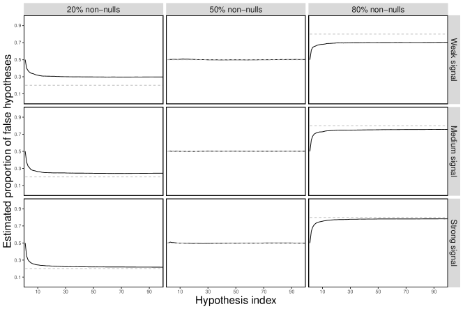
Figure 1: Comparing $\hat{\tau}_{i}$ (solid line) defined in (9) to the true $\tau_{i}$ (dashed line) for different scenarios. The simulation design is described in Section 4. The estimate $\hat{\tau}_{i}$ has a tendency to bias towards $50\%$ but it estimates the proportion of false hypotheses very well when the signal is strong.

Hedging the e-values before multiplying them does not only apply to GRO e-values. Such strategies for merging sequential e-values have been used by many preceding authors like Waudby-Smith and Ramdas [46], Vovk and Wang [41]. However, the above argumentation provides a reasonable choice for the parameter $\lambda_{i}$ in our setting.

We analyze this approach experimentally in Section 4.2.

3.3 Calibrating sequential p-values into e-values

While e-values have been of recent interest, most studies still use p-values as measure of evidence against the null hypothesis. In this case, we can calibrate the p-values into e-values and then apply SeqE-Guard. In this context, a calibrator is a function from p-values to e-values, meaning it takes as an input a p-value and yields an e-value as an output.

For example, the online-simple method of Katsevich and Ramdas [21] introduced in Section 3.1 is implicitly based on calibrating each p-value into a simple binary e-value. However, there are infinitely many other calibrators that could be used. Assume that p-values $(P_{t})_{t\in\mathbb{N}}$ for the hypotheses $(H_{t})_{t\in\mathbb{N}}$ are given. A decreasing function $f:[0,1]\rightarrow[0,\infty]$ is a calibrator if $\int_{0}^{1}f(x)dx\leq 1$, and it is admissible if equality holds [42, 39]. Note that if the p-values are sequential p-values, meaning $P_{t}$ is measurable with respect to $\mathcal{F}_{t}$ and $\mathbb{P}(P_{t}\leq x|\mathcal{F}_{t-1})\leq x$ for all $x\in[0,1]$, then the calibrated e-values are sequential e-values.

An example calibrator is

$$h_{x}(p)=\exp\left(x\Phi^{-1}(1-p)-x^{2}/2\right),$$ (10)

where $\Phi$ denotes the CDF of a standard normal distribution. To see that this is a valid calibrator, note that $\Phi^{-1}(U)$, where $U\sim[0,1]$, follows a standard normal distribution and the moment generating function of a standard normal distribution for the real parameter $x>0$ is given by $\exp(x^{2}/2)$. Duan et al. [7] used this calibrator to derive a martingale Stouffer [36] global test. This global test is based on a confidence sequence of Howard et al. [19].

We compare the application of SeqE-Guard with calibrated e-values, GRO e-values and the e-values defined by Katsevich and Ramdas [21] experimentally in Section 4.3.

3.4 Boosting of sequential e-values

Wang and Ramdas [44] introduced a way to boost e-values before plugging them into their e-BH procedure without violating the desired FDR control. In this section, we propose a similar (but simpler) approach for SeqE-Guard that will improve its power even further.

We begin by noting that whenever the bound $d_{t}$ is increased by one, the largest e-value with index in $A$ will not be considered in the following analysis. Hence, extremely large e-values will be excluded from the analysis anyway, which makes it possible to truncate the e-values at a specific threshold without changing its outcome. This makes the resulting truncated e-values conservative under the null, and one can improve the procedure by multiplying the e-value by a suitable constant larger than 1 to remove its conservativeness. This truncation+multiplication operation is what is referred to as boosting the e-value.

To this end, recall that $A_{t-1}\subseteq R_{t-1}$, $t\in\mathbb{N}$, is the index set of all previous e-values in the rejection set that were not already excluded by SeqE-Guard and $U_{t-1}\subseteq\{1,\ldots,t-1\}\setminus R_{t-1}$ the index set of all previous e-values that are not contained in the rejection set and that are smaller than $1$. Now, define

$$m_{t}:=\max\left\{\max_{i\in A_{t-1}}E_{i},\frac{1}{\alpha\prod_{i\in A_{t-1}\cup U_{t-1}}E_{i}}\right\},$$ (11)

and note that $m_{t}$ is predictable (measurable with respect to $\mathcal{F}_{t-1}$). Furthermore, if $E_{t}\geq m_{t}$ and $t\in R_{t}$, then $d_{t}=d_{t-1}+1$ and $E_{t}$ will be excluded in the further analysis. If $E_{t}\geq m_{t}$ and $t\notin R_{t}$, then $E_{t}\geq 1$, since $m_{t}\geq 1$ by definition, and $E_{t}$ won’t be considered in the analysis anyway. Hence, we define the truncation function $T_{t}:[0,\infty]\rightarrow[0,m_{t}]$ as

$$T_{t}(x):=x\mathbbm{1}\{x\leq m_{t}\}+m_{t}\mathbbm{1}\{x>m_{t}\}$$ (12)

and then choose a boosting factor $b_{t}\geq 1$ as large as possible such that

$$\mathbb{E}_{\mathbb{P}}[T_{t}(b_{t}E_{t})|\mathcal{F}_{t-1}]\leq 1\text{ for all }\mathbb{P}\in H_{t}.$$ (13)

Note that $b_{t}=1$ always satisfies (13); so a boosting factor always exists and is always at least one. Condition (13) immediately implies that $T_{t}(b_{t}E_{t})$ is a sequential e-value. Furthermore, using $b_{t}E_{t}$ in SeqE-Guard yields exactly the same results as using $T_{t}(b_{t}E_{t})$. Therefore, applying SeqE-Guard to the boosted e-values $(b_{t}E_{t})_{t\in\mathbb{N}}$ provides simultaneous true discovery guarantee and is uniformly more powerful than with non-boosted e-values, since $b_{t}\geq 1$. Note that in this case $m_{t}$ should also be calculated based on the boosted e-values $b_{1}E_{1},\ldots,b_{t-1}E_{t-1}$. As also mentioned by Wang and Ramdas [44], one could use different functions than $x\mapsto bx$ for some $b\geq 1$ to boost the e-values. In general, it is only required that each boosted e-value $E_{t}^{\mathrm{boost}}$, $t\in\mathbb{N}$, satisfies $\mathbb{E}_{\mathbb{P}}[T_{t}(E_{t}^{\mathrm{boost}})|\mathcal{F}_{t-1}]\leq 1$ for all $\mathbb{P}\in H_{t}$. We summarize this result in the following theorem.

Theorem 3.3.

Let $E_{1}^{\mathrm{boost}},E_{2}^{\mathrm{boost}},\ldots$ be a sequence of nonnegative random variables such that $\mathbb{E}_{\mathbb{P}}[T_{t}(E_{t}^{\mathrm{boost}})|\mathcal{F}_{t-1}]\leq 1$ for all $\mathbb{P}\in H_{t}$, where $T_{t}$ is given by (12) and $m_{t}$ is calculated as in (11) based on $E_{1}^{\mathrm{boost}},\ldots,E_{t-1}^{\mathrm{boost}}$. Then, applying SeqE-Guard to the boosted sequential e-values $E_{1}^{\mathrm{boost}},E_{2}^{\mathrm{boost}},\ldots$ provides simultaneous true discovery guarantee.

In the following we provide several examples that illustrate how the boosting factors can be determined in specific cases and demonstrate the possible gain in efficiency.

Example 2.

We consider Example 3 from Wang and Ramdas [44] adapted to our setting. For each $t\in\mathbb{N}$, we test the simple null hypothesis $H_{t}:X_{t}|\mathcal{F}_{t-1}\sim\mathcal{N}(\mu_{0},1)$ against the simple alternative $H_{t}^{A}:X_{t}|\mathcal{F}_{t-1}\sim\mathcal{N}(\mu_{1},1)$, where $X_{t}$ denotes the data for $H_{t}$. In this case, the GRO e-value is given by the likelihood ratio between two normal distributions with variance $1$ and means $\mu_{1}$ and $\mu_{0}$

$$E_{t}=\exp(\delta Z_{t}-\delta^{2}/2),$$ (14)

where $\delta=\mu_{1}-\mu_{0}>0$ and $Z_{t}=X_{t}-\mu_{0}$ follows a standard normal distribution conditional on $\mathcal{F}_{t-1}$ under $H_{t}$. Hence, conditional on the past, each null e-value follows a log-normal distribution with parameter $(-\delta^{2}/2,\delta)$. With this, we obtain for all $t\in I_{0}^{\mathbb{P}}$:

$$\mathbb{E}_{\mathbb{P}}[b_{t}E_{t}\mathbbm{1}\{b_{t}E_{t}\leq m_{t}\}+m_{t}\mathbbm{1}\{b_{t}E_{t}>m_{t}\}|\mathcal{F}_{t-1}]$$

$$=b_{t}\mathbb{E}_{\mathbb{P}}[E_{t}\mathbbm{1}\{b_{t}E_{t}\leq m_{t}\}|\mathcal{F}_{t-1}]+m_{t}\mathbb{P}(b_{t}E_{t}>m_{t}|\mathcal{F}_{t-1})$$

$$=b_{t}\left[1-\Phi\left(\frac{\delta}{2}-\frac{\log\left(m_{t}/b_{t}\right)}{\delta}\right)\right]+m_{t}\left[1-\Phi\left(\frac{\log(m_{t}/b_{t})+\delta^{2}/2}{\delta}\right)\right],$$

where $\Phi$ is the CDF of a standard normal distribution. The last expression can be set equal to $1$ and then be solved for $b_{t}$ numerically. For example, for $\delta=3$ and $m_{t}=20$, we obtain $b_{t}=3.494$. Hence, the e-value $E_{t}$ could be multiplied by $3.494$ without violating the true discovery guarantee, a substantial gain. In general, the larger $m_{t}$, the smaller is the boosting factor. For example, if $m_{t}=5$, then $b_{t}=11.826$ and if $m_{t}=100$, then $b_{t}=1.774$. Nevertheless, even the latter boosting factor would increase the power of the true discovery procedure significantly and we would usually expect $m_{t}$ to be smaller than $100$ in most settings. If we use, as described in Section 3.2, the e-value $1-\lambda_{t}+\lambda_{t}E_{t}^{\mathrm{GRO}}$, $\lambda_{t}\in(0,1)$ instead, we need to solve

$$b_{t}(1-\lambda_{t})\Phi\left(\frac{\log(s_{t})+\delta^{2}/2}{\delta}\right)+b_{t}\lambda_{t}\left[1-\Phi\left(\frac{\delta}{2}-\frac{\log\left(s_{t}\right)}{\delta}\right)\right]+m_{t}\left[1-\Phi\left(\frac{\log(s_{t})+\delta^{2}/2}{\delta}\right)\right]=1,$$

for $b_{t}\in[1,1/(1-\lambda_{t}))$, where $s_{t}=(\lambda_{t}-1+m_{t}/b_{t})/\lambda_{t}$. In this case, $\delta=3$, $\lambda_{t}=0.5$ and $m_{t}=20$ yield a boosting factor of $b_{t}=1.354$.

Example 3.

Suppose we observe sequential p-values $P_{1},P_{2},\ldots$ and want to apply the calibrator (10). If the p-values are uniformly distributed conditional on the past, the resulting e-value has the exact same distribution as the e-value in (14) under the null hypothesis for $\delta=x$, where $x$ is the freely chosen parameter for the calibrator. Hence, we can do the exact same calculations to obtain an appropriate boosting factor. If the p-values are stochastically larger than uniform, we could still use that same boosting factor, as the resulting e-values provide true discovery guarantee but might be conservative.

Example 4.

In case of the closed online-simple method (Algorithm 2) it is particular simple to “boost” the e-values. Since $E_{i}^{\mathrm{os}}$ only takes two different values, we can simply ensure $E_{t}^{\mathrm{os}}\leq m_{t}$ by choosing $\alpha_{t}$ appropriately. Note that in case of $\alpha_{t}=\alpha$ for all $t\in\mathbb{N}$ it is not possible to improve the bounds of the closed online-simple method further by boosting, since we already have $E_{t}^{\mathrm{os}}\leq m_{t}$ almost surely.

In their Example 2, Wang and Ramdas [44] showed how a boosting factor for their e-BH method can be obtained when using a different calibrator. Similar calculations can be done for our truncation function.

4 Simulations

In this section we numerically calculate the true discovery proportion (TDP) bound, which is defined as the true discovery bound for $R_{t}$ divided by the size of $R_{t}$. We compare TDP bounds obtained by applying SeqE-Guard to the different sequential e-values proposed in the previous sections. In Subsection 4.1, we compare the online-simple method by Katsevich and Ramdas [21] with its uniform improvement. In Subsection 4.2 we demonstrate how hedging and boosting GRO e-values improve the true discovery bound. Finally, in Subsection 4.3, we compare all the proposed e-values to decide which is best suited for practice.

We consider the same simulation setup in all subsections. We sequentially test $n=1000$ null hypotheses $H_{i}$, $i\in\{1,\ldots,n\}$, of the from $H_{i}:X_{i}\sim\mathcal{N}(0,1)$ against the alternative $H_{i}^{A}:X_{i}\sim\mathcal{N}(\mu_{A},1)$ for some $\mu_{A}>0$, where $X_{1},\ldots,X_{n}$ are independent data points or test statistics. The probability that a hypothesis is true is set by a parameter $\pi_{A}\in(0,1)$ and the desired guarantee is set to $\alpha=0.1$. For all comparisons we consider a grid of simulation parameters $\mu_{A}\in\{2,3,4\}$ and $\pi_{A}\in\{0.1,0.3,0.5\}$, where we refer to $\mu_{A}=2$ as weak signal, $\mu_{A}=3$ as medium signal and $\mu_{A}=4$ as strong signal. The p-values are calculated by $\Phi(-X_{i})$, where $\Phi$ is the CDF of a normal distribution. The raw GRO e-values are given by the likelihood ratio $E_{i}^{\mathrm{GRO}}=p_{\mu_{A}}(X_{i})/p_{0}(X_{i})$, where $p_{\mu_{A}}$ and $p_{0}$ are the densities of a normal distribution with variance $1$ and mean $\mu_{A}$ and $0$, respectively. The rejection sets $R_{t}$, $t\in\{1,\ldots,t\}$, are defined as $R_{t}=\{i\in\{1,\ldots,t\}:P_{i}\leq\alpha\}$. All of the results in the following are obtained by averaging over $1000$ independent trials.

4.1 Comparing the online-simple method [21] with its improvements

In Section 3.1 we showed that the online-simple method by Katsevich and Ramdas [21] can be uniformly improved by the closed online-simple procedure (Algorithm 2). We also showed that this closed procedure can be further uniformly improved by the admissible online-simple procedure, which ensures that the expected value of each sequential e-value is exactly one. In this section, we aim to quantify the gain in power for making true discoveries by using these improvements instead of the online-simple method.

The results are illustrated in Figure 2. It can be seen that the closed online-simple procedure leads to substantial improvements of the online-simple procedure in all cases. Of the rejected hypotheses, the former approximately identifies $20\%$ more as truly false. Also note that when only $10\%$ of the hypotheses are false, the true discovery bound of the original online-simple method is trivial.

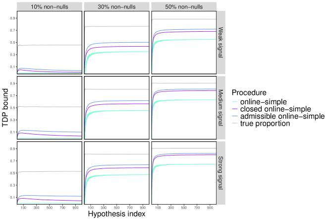
Figure 2: True discovery proportion bounds obtained by the online-simple method [21], the closed online-simple method and the admissible online-simple method. The closed online-simple method leads to substantially larger bounds than the original online-simple method. An additional improvement can be obtained by the admissible online-simple method, which is closest to the true proportion (top line) in all figures.

4.2 GRO e-values

In Section 3.2 we argued that the raw GRO e-values should be hedged to account for the probability that a null hypothesis is true. In Section 3.4 we showed how the (hedged) GRO e-values can be boosted by truncating them to avoid an overshoot. This leads to a uniform improvement compared to using the raw (hedged) e-values. In this section, we compare the true discovery bounds obtained by applying SeqE-Guard to raw, hedged and boosted GRO e-values. Note that the boosted e-values were obtained by applying the boosting technique to the hedged GRO e-values. For the hedged GRO e-values we chose the predictable parameter proposed in (9).

The results are illustrated in Figure 3. The raw GRO e-values lead to very low bounds. However, these can be increased substantially by hedging the GRO e-values before plugging them into SeqE-Guard. The bounds obtained by hedged GRO e-value can further be significantly improved by boosting.

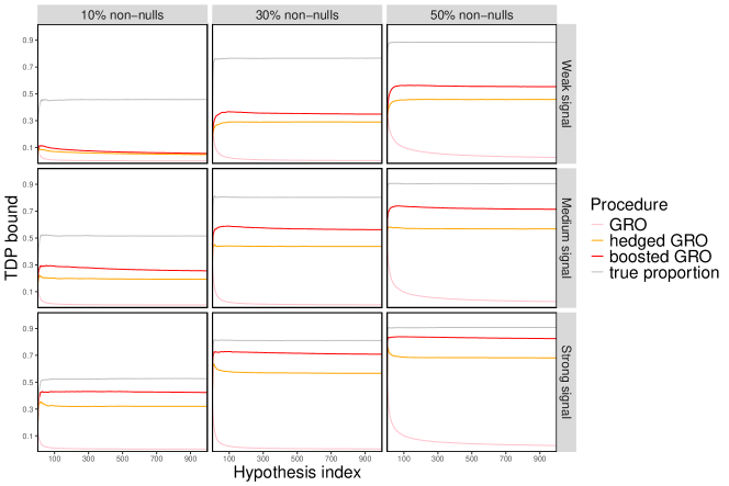
Figure 3: True discovery proportion bounds obtained by applying SeqE-Guard to GRO e-values, hedged GRO e-values and boosted GRO e-values. The hedged GRO e-values improve the GRO e-values substantially. An additional significant improvement is obtained by boosting.

4.3 Which sequential e-values should we choose?

In this section, we compare the SeqE-Guard procedure when applied with the best versions of the proposed sequential e-values to derive recommendations for practice. We compare the admissible online-simple method, the boosted GRO e-value and the calibrated e-value with the calibrator defined in (10). For the calibrated method we chose the parameter $x=0.1$ and boosted the e-values as described in Example 3.

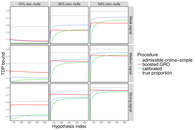
Figure 4: True discovery proportion bounds obtained by the admissible online-simple method, applying SeqE-Guard to boosted GRO e-values and applying SeqE-Guard to calibrated e-values. When the signal is strong, the boosted GRO e-values perform best, particularly, if the proportion of false hypotheses is small. If the signal is weak but the proportion of false hypotheses is large, the admissible online-simple method leads to a larger bound.

The results are depicted in Figure 4. The procedures perform quite different in the various settings. When the signal is strong, the SeqE-Guard algorithm performs best with boosted GRO e-values, particularly, if the proportion of false hypotheses is small. Indeed, in case of $\mu_{A}=4$ and $\pi_{A}=0.1$, the boosted GRO e-value leads to a fairly tight bound, while the calibrated e-values and the admissible online-simple algorithm have problems with detecting any false hypotheses. However, if the proportion of false hypotheses is large but the signal is weak, the admissible online-simple method clearly outperforms the SeqE-Guard with boosted GRO e-values. The calibrated e-values did not lead to the largest bound in any case. Hence, if we expect sparse but strong signal, applying SeqE-Guard with boosted GRO e-values is the best choice. In contrast, for dense but weak signals, the admissible online-simple method should be preferred. If not any prior information is available, we would recommend to apply the SeqE-Guard algorithm with GRO e-values, since they showed the best performance overall and provided reasonable bounds in any case. Furthermore, we would like to point out that all the proposed methods show remarkable long-term behavior, as the TDP bound becomes approximately constant towards the end. Consequently, the proposed methods are well-suited for large scale multiple testing problems, as they often occur in online applications.

5 Online true discovery guarantee under arbitrary dependence

In the previous sections we explored an online true discovery procedure that works for sequential e-values. While we believe that this is a very common situation for many online applications, there are also cases where no information about the dependence structure is available. This typically occurs when data is reused for multiple hypotheses. For example, this is the case when open data repositories are evaluated in different studies [27, 5] or in Kaggle competitions [3]. In addition, arbitrarily dependent test statistics occur when the data for multiple hypotheses is collected from the same subpopulation, as it can be the case in online A/B testing [23]. For this reason, in this section we propose a method for online true discovery guarantee that works under arbitrary dependence of the e-values. We just assume that each e-value $E_{i}$ for $H_{i}$ is measurable with respect to $\mathcal{F}_{i}$, which is needed to define an online procedure based on these e-values.

While (hedged) multiplication is the admissible way of combining sequential e-values [41], Vovk and Wang [39] showed that the average is the only admissible symmetric merging function for arbitrarily dependent e-values. Therefore, it seems evident to look at averages when constructing intersection tests for arbitrarily dependent e-values. However, since we consider online true discovery guarantee, it is not possible to use the symmetric average.

Example 5.

Consider the intersection hypotheses $H_{\{1\}}$ and $H_{\{1,2\}}$ and suppose we test each of these using the (unweighted) average of two e-values $E_{1}$ and $E_{2}$. That means, $\phi_{\{1\}}=1$ if $E_{1}\geq 1/\alpha$ and $\phi_{\{1,2\}}=1$ if $(E_{1}+E_{2})/2\geq 1/\alpha$. Suppose $1/\alpha\leq E_{1}<2/\alpha-E_{2}$. Then $\phi_{\{1\}}=1$ but $\phi_{\{1,2\}}=0$, implying that $\boldsymbol{\phi}=(\phi_{I})_{I\subseteq\mathbb{N}}$ is not increasing and the resulting closed procedure is not an online procedure. Also note that it is not possible to apply the unweighted average for an infinite number of hypotheses.

For this reason, we will focus on weighted averages. To this regard, prespecify a nonnegative sequence $(\gamma_{i})_{i\in\mathbb{N}}$ with $\sum_{i\in\mathbb{N}}\gamma_{i}=1$. Then for each $I\subseteq\mathbb{N}$, define the intersection test

$$\phi_{I}=\mathbbm{1}\left\{\sum_{i\in I}E_{i}\gamma_{t(i;I)}\geq 1/\alpha\right\},$$ (15)

where $t(i;I)=|\{j\in I:j\leq i\}|$. For every $I\subseteq\mathbb{N}$, we have

$$\mathbb{E}_{\mathbb{P}}\left[\sum_{i\in I}E_{i}\gamma_{t(i;I)}\right]=\sum_{i\in I}\gamma_{t(i;I)}\mathbb{E}_{\mathbb{P}}\left[E_{i}\right]\leq\sum_{i\in I}\gamma_{t(i;I)}\leq 1\quad(\mathbb{P}\in H_{I}),$$

implying that $\sum_{i\in I}E_{i}\gamma_{t(i;I)}$ is a valid e-value for $H_{I}$. By Markov’s inequality, $\phi_{I}$ in (15) defines an $\alpha$-level intersection test. Furthermore, if $I\subseteq\{1,\ldots,i\}$ and $K=I\cup J$ for some $J\subseteq\{j\in\mathbb{N}:j>i\}$, then $t(l;I)=t(l;K)$ for all $l\in I$, which implies that $\boldsymbol{\phi}=(\phi_{I})_{I\subseteq\mathbb{N}}$ is increasing. Since each $\phi_{I}$ is additionally an online intersection test, the closed procedure based on the intersection tests in (15) is an online true discovery procedure under arbitrary dependence of the e-values.

One problem with such weighted methods is that it is difficult to find a short-cut for the corresponding closed procedure in general. In Algorithm 3 we provide a conservative short-cut, if $(\gamma_{i})_{i\in\mathbb{N}}$ is nonincreasing (we call the Algorithm ArbE-Guard). That means, the true discovery bounds provided by the short-cut are always smaller than or equal to the bounds of the exact closed procedure and therefore it also provides simultaneous true discovery guarantee. The idea of the short-cut is to make the conservative assumption that all e-values that are not contained in the rejection set equal $0$. Hence, if we choose loose criteria for including an index in the rejection set, the short-cut will be close to the full closed procedure based on (15). For example, if we just want a lower bound for the number of false hypotheses among all hypotheses under consideration, the short-cut is exact. However, if we choose strict criteria for including indices in the rejection set, e.g., if we desire FWER control, then the short-cut is conservative.

Theorem 5.1.

Let $E_{1},E_{2},\ldots$ be arbitrarily dependent e-values for $H_{1},H_{2},\ldots$ . The true discovery bounds $d_{t}$ for $R_{t}$ defined by ArbE-Guard (Algorithm 3) satisfy $d_{t}\leq\boldsymbol{d}^{\boldsymbol{\phi}}(R_{t})$ for all $t\in\mathbb{N}$, where $\boldsymbol{d}^{\boldsymbol{\phi}}$ is the online closed procedure based on the intersection tests defined in (15). In particular, $R_{t}$ and $d_{t}$ satisfy for all $\mathbb{P}\in\mathcal{P}$: $\mathbb{P}(d_{t}\leq|R_{t}\cap I_{1}^{\mathbb{P}}|\text{ for all }t\in\mathbb{N})\geq 1-\alpha$.

Algorithm 3 ArbE-Guard: Online true discovery guarantee with arbitrarily dependent e-values

Input: Nonnegative and nonincreasing sequence $(\gamma_{i})_{i\in\mathbb{N}}$ with $\sum_{i\in\mathbb{N}}\gamma_{i}\leq 1$ and sequence of (possibly) arbitrarily dependent e-values $E_{1},E_{2},\ldots$ .
      Output: Rejection sets $R_{1}\subseteq R_{2}\subseteq\ldots$ and true discovery bounds $d_{1}\leq d_{2}\leq\ldots$ .

1:$d_{0}=0$

2:$R_{0}=\emptyset$

3:$A^{c}=\emptyset$

4:for $t=1,2,\ldots$ do

5:     $R_{t}=R_{t-1}$

6:     $d_{t}=d_{t-1}$

7:     Observe $E_{t}$ and decide whether $t$ should be included in $R_{t}$.

8:     if $t\in R_{t}$ then

9:         if $\sum_{i\in R_{t}\setminus A^{c}}E_{i}\gamma_{t(i;\{1,\ldots,t\}\setminus A^{c})}\geq 1/\alpha$ then

10:              $d_{t}=d_{t-1}+1$

11:              $A^{c}=A^{c}\cup\left\{\operatorname*{argmin}_{i\in R_{t}\setminus A^{c}}\sum_{j\in R_{t}\setminus[A^{c}\cup\{i\}]}E_{j}\gamma_{t(j;\{1,\ldots,t\}\setminus[A^{c}\cup\{i\}])}\right\}$

12:         end if

13:     end if

14:     return $R_{t},d_{t}$

15:end for

Remark 3.

Note that if $E_{t}\geq\frac{1}{\alpha\gamma_{t}}$, the bound $d_{t}$ obtained by ArbE-Guard will be increased by one and the e-value $E_{t}$ excluded from the future analysis. Hence, we could truncate $E_{t}$ at the value $\frac{1}{\alpha\gamma_{t}}$ and exploit this for boosting $E_{t}$ similarly as described for sequential e-values in Section 3.4. However, note that we are not allowed to use any information about the previous e-values to increase the boosting factor due to the dependency between the e-values. Also note that $\frac{1}{\alpha\gamma_{t}}$ is usually much larger than the cutoff $m_{t}$ (11) defined for sequential e-values, which is why the boosting factors will be smaller.

6 Discussion

In this paper, we proposed a new closed testing based online true discovery procedure for sequential e-values and derived a general short-cut that only requires one calculation per hypothesis. Although the SeqE-Guard algorithm is restricted to sequential e-values, it is a general procedure for the task of online true discovery guarantee, since there are many different ways to construct sequential e-values. In fact, we even wonder whether there is any true discovery procedure for the online setting where we observe an independent data set for each hypothesis that is not uniformly improved by SeqE-Guard. This conjecture is based on our theoretical result that test martingales are required for online true discovery guarantee and the close connection between e-values and test martingales. Furthermore, the only existing procedures for this task introduced by Katsevich and Ramdas [21] were easily improved by SeqE-Guard, although they were not explicitly constructed using e-values.

From a theoretical point of view this paper gives new insights about the role of e-values in multiple testing by demonstrating their value for online true discovery guarantee. From a practical point of view, we constructed a powerful and flexible multiple testing procedure, which allows to observe hypotheses one-by-one over time and make fully data-adaptive decisions about the hypotheses and stopping time while bounding the number of true discoveries or equivalently, the false discovery proportion. On the way, we introduced new ideas for hedging and boosting of sequential e-values. These approaches similarly apply to global testing and anytime-valid testing of a single hypothesis, which could be explored in future work.

Although not being the main focus of this paper, we also introduced a new method with online true discovery guarantee for the setting of arbitrarily dependent e-values. To the best of our knowledge, this is the first approach in this setting and therefore provides the new benchmark for future work.

Acknowledgments

LF acknowledges funding by the Deutsche Forschungsgemeinschaft (DFG, German Research Foundation) – Project number 281474342/GRK2224/2. AR was funded by NSF grant DMS-2310718.

Appendix A Uniform improvement of the online-adaptive method by Katsevich and Ramdas [21]

Let p-values $P_{1},P_{2},\ldots$ and significance levels $\alpha_{1},\alpha_{2},\ldots$ be defined as for the online-simple algorithm (see Section 3.1), and the null p-values be valid conditional on the past. Furthermore, let $(\lambda_{i})_{i\in\mathbb{N}}$ be additional parameters such that $\lambda_{i}\in[\alpha_{i},1)$ is measurable with respect to $\mathcal{F}_{i-1}$ and $B:=\sup_{i\in\mathbb{N}}\frac{\alpha_{i}}{1-\lambda_{i}}<\infty$. The online-adaptive bound by Katsevich and Ramdas [21]

$$d^{\text{ad}}(R_{t})=\left\lceil-ca+\sum_{i=1}^{t}\mathbbm{1}\{P_{i}\leq\alpha_{i}\}-c\frac{\alpha_{i}}{1-\lambda_{i}}\mathbbm{1}\{P_{i}>\lambda_{i}\}\right\rceil$$

provides simultaneous true discovery guarantee over all sets $R_{t}=\{i\leq t:P_{i}\leq\alpha_{i}\}$, $t\in\mathbb{N}$, where $a>0$ is some regularization parameter and $c=\frac{\log(1/\alpha)}{a\log(1+(1-\alpha^{B/a})/B)}$. Note that $c$ has a different value than for the online-simple algorithm. Similar as demonstrated in Section 3.1, Katsevich and Ramdas [21] proved the error guarantee by showing that $E_{i}^{\text{ad}}=\exp[\theta_{c}(\mathbbm{1}\{P_{i}\leq\alpha_{i}\}-c\frac{\alpha_{i}}{1-\lambda_{i}}\mathbbm{1}\{P_{i}>\lambda_{i}\})]$, $i\in\mathbb{N}$, are sequential e-values, where $\theta_{c}=\log(1/\alpha)/(ca)$. Note that

$$\prod_{i\in I}E_{i}^{\text{ad}}\geq 1/\alpha\Leftrightarrow\sum_{i\in I}\mathbbm{1}\{P_{i}\leq\alpha_{i}\}-c\frac{\alpha_{i}}{1-\lambda_{i}}\mathbbm{1}\{P_{i}>\lambda_{i}\}\geq\log(1/\alpha)/\theta_{c}=ca\quad(I\in 2^{\mathbb{N}_{f}}).$$

With this, one can define a uniform improvement of the online-adaptive algorithm in the exact same manner as for the online-simple algorithm. Note that the online-adaptive method already adapts to the proportion of null hypotheses using the parameter $\lambda_{i}$ and therefore cannot be further improved by the (online) closure principle in that direction. However, it still leads to a real uniform improvement by transforming it into a coherent procedure. Furthermore, the e-values $E_{i}^{\text{ad}}$ are inadmissible if $\alpha_{i}/(1-\lambda_{i})$ is not constant for all $i\in\mathbb{N}$ and thus can be improved. For this, note that $E_{i}^{\text{ad}}=\exp(\theta_{c})$, if $P_{i}\leq\alpha_{i}$, $E_{i}^{\text{ad}}=1$, if $\alpha_{i}<P_{i}\leq\lambda_{i}$ and $E_{i}^{\text{ad}}=\exp(-\theta_{c}c\alpha_{i}/(1-\lambda_{i}))$, if $P_{i}>\lambda_{i}$. Hence, for all $\mathbb{P}\in H_{i}$, we can provide a tight upper bound for the expectation of $E_{i}^{\text{ad}}$ by

$$\mathbb{E}_{\mathbb{P}}[E_{i}^{\text{ad}}|\mathbb{F}_{i-1}] =\exp(\theta_{c})\mathbb{P}(P_{i}\leq\alpha_{i}|\mathcal{F}_{i-1})+\mathbb{P}(\alpha_{i}<P_{i}\leq\lambda_{i}|\mathcal{F}_{i-1})+\exp\left(-\theta_{c}c\frac{\alpha_{i}}{1-\lambda_{i}}\right)\mathbb{P}(P_{i}>\lambda_{i}|\mathcal{F}_{i-1})$$

$$=(\exp(\theta_{c})-1)\mathbb{P}(P_{i}\leq\alpha_{i}|\mathcal{F}_{i-1})+\mathbb{P}(P_{i}\leq\lambda_{i}|\mathcal{F}_{i-1})\left[1-\exp\left(-\theta_{c}c\frac{\alpha_{i}}{1-\lambda_{i}}\right)\right]+\exp\left(-\theta_{c}c\frac{\alpha_{i}}{1-\lambda_{i}}\right)$$

$$\leq(\exp(\theta_{c})-1)\alpha_{i}+\lambda_{i}\left[1-\exp\left(-\theta_{c}c\frac{\alpha_{i}}{1-\lambda_{i}}\right)\right]+\exp\left(-\theta_{c}c\frac{\alpha_{i}}{1-\lambda_{i}}\right)=:u(\alpha,\alpha_{i},\lambda_{i},B,a),$$

which can easily be calculated for given $\alpha$, $\alpha_{i}$, $\lambda_{i}$, $B$ and $a$. If $B=\alpha_{i}/(1-\lambda_{i})$, then $u(\alpha,\alpha_{i},\lambda_{i},B,a)=1$. However, in practice $\alpha_{i}/(1-\lambda_{i})$ may vary over time such that there are indices $j\in\mathbb{N}$ with $\alpha_{j}/(1-\lambda_{j})<1$. In this case, the e-value $E_{j}^{\text{ad}}$ becomes conservative. For example, if $\alpha=0.1$, $\alpha_{i}=0.1$, $\lambda_{i}=0.5$, $B=0.4$ and $a=1$, then $u(\alpha,\alpha_{i},\lambda_{i},B,a)=0.966$.

Appendix B Proofs

Proof of Theorem 2.1.

The simultaneous true discovery guarantee of $\boldsymbol{d}$ implies that the $\phi_{I}$ define $\alpha$-level intersection tests. Furthermore, it follows that $\boldsymbol{\phi}$ is increasing since $\boldsymbol{d}$ is coherent and $\phi_{S}$ is an online intersection test since $\boldsymbol{d}$ is an online procedure. Therefore, it only remains to show that $\boldsymbol{d}(S)\leq\boldsymbol{d}^{\boldsymbol{\phi}}(S)$ for all $S\in 2^{\mathbb{N}_{f}}$. Suppose $\boldsymbol{d}(S)=s$. Due to the coherence of $\boldsymbol{d}$, we have $\phi_{J}=1$ for all $J\subseteq S$ with $|J|>|S|-s$. The coherence further implies that $\phi_{I}=1$ for all $I\subseteq\mathbb{N}$ with $|S\cap I|>|S|-s$ and hence $\boldsymbol{d}^{\boldsymbol{\phi}}(S)\geq s$. ∎

Proof of Theorem 2.2.

Since $\phi_{I\cap\{1,\ldots,i\}}$ is an online intersection test, we have that $\psi^{I}_{i}$ is measurable with respect to $\mathcal{F}_{i}$. Furthermore, since $\boldsymbol{\phi}$ is increasing, it holds for every stopping time $\tau$ that $\mathbb{P}(\psi^{I}_{\tau}=1)\leq\mathbb{P}(\phi_{I}=1)\leq\alpha$ for all $\mathbb{P}\in H_{I}$. Hence, $(\psi^{I}_{i})_{i\in I}$ is an anytime-valid test for $H_{I}$ with respect to the filtration $(\mathcal{F}_{i})_{i\in I}$. ∎

Proof of Theorem 2.3.

Define $\phi_{S}$, $S\in 2^{\mathbb{N}_{f}}$, and $\phi_{J}$, $J\in 2^{\mathbb{N}_{-f}}$, as in (5). For all $J\in 2^{\mathbb{N}_{-f}}$, let $\psi_{i}^{J}=\max\{\phi_{S}:S\subseteq J\cap\{1,\ldots,i\},S\in 2^{\mathbb{N}_{f}}\}$. Then $(\psi_{i}^{J})_{i\in J}$ is an anytime-valid test for $H_{J}$ with respect to $(\mathcal{F}_{i})_{i\in J}$ and $\phi_{J}=(\psi_{i}^{J})_{i\in J}$. If $(\psi_{i}^{J})_{i\in J}$ is admissible for all $J\in 2^{\mathbb{N}_{-f}}$, we are done. Otherwise, since $\mathcal{P}$ is locally dominated [29], we can find an admissible $(\tilde{\psi}_{i}^{J})_{i\in J}$ that uniformly improves $(\psi_{i}^{J})_{i\in J}$. Now, let $\tilde{\phi}_{I}=\phi_{I}$, if $I$ is finite or $(\psi_{i}^{J})_{i\in J}$ is admissible, and $\tilde{\phi}_{I}=(\tilde{\psi}_{i}^{I})_{i\in I}$ otherwise. Then $\tilde{\boldsymbol{\phi}}=(\tilde{\phi}_{I})_{I\subseteq\mathbb{N}}$ is an increasing family of online intersection tests and $\boldsymbol{d}^{\tilde{\boldsymbol{\phi}}}(S)=\boldsymbol{d}(S)$ for all $S\in 2^{\mathbb{N}_{-f}}$. ∎

Proof of Theorem 3.1.

Let $d_{t}$, $t\in\mathbb{N}$, be the bounds of SeqE-Guard, $A_{t}\subseteq R_{t}$ be the set $A$ at time $t$ before checking whether $\Pi_{A\cup U}\geq 1/\alpha$, $U_{t}\subseteq\{1,\ldots,t\}\setminus R_{t}$ the index set of e-values that are smaller than $1$ and $\Pi_{Z}$, $Z\subseteq\mathbb{N}$, be the product of all e-values with index in $Z$. Since $\boldsymbol{\phi}$ is increasing, we have $d_{1}=\boldsymbol{d}^{\boldsymbol{\phi}}(R_{1})$. Now assume that $d_{1}=\boldsymbol{d}^{\boldsymbol{\phi}}(R_{1}),\ldots,d_{t-1}=\boldsymbol{d}^{\boldsymbol{\phi}}(R_{t-1})$ and $R_{t}=R_{t-1}\cup\{t\}$. Due to the coherence of $\boldsymbol{d}^{\boldsymbol{\phi}}$, it holds $d_{t-1}\leq\boldsymbol{d}^{\boldsymbol{\phi}}(R_{t})\leq d_{t-1}+1$. In the following, we show that $\Pi_{A_{t}\cup U_{t}}\geq 1/\alpha$ implies that $\boldsymbol{d}^{\boldsymbol{\phi}}(R_{t})\geq d_{t-1}+1$ and $\Pi_{A_{t}\cup U_{t}}<1/\alpha$ implies that $\boldsymbol{d}^{\boldsymbol{\phi}}(R_{t})<d_{t-1}+1$, which proves the assertion.

We first show that $\boldsymbol{d}^{\boldsymbol{\phi}}(R_{t})\geq d_{t-1}+1$, if $\Pi_{A_{t}\cup U_{t}}\geq 1/\alpha$. For this, we prove that $\Pi_{A_{t}\cup U_{t}}\geq 1/\alpha$ implies $\phi_{I}=1$ for all $I=V\cup W$, where $V\subseteq R_{t}$ and $W\subseteq\{1,\ldots,t\}\setminus R_{t}$ with $|V|\geq|A_{t}|$. Since $\boldsymbol{\phi}$ is increasing, we have $\boldsymbol{d}^{\boldsymbol{\phi}}(R_{t})=\min\{|R_{t}\setminus I|:I\subseteq\{1,\ldots,t\},\phi_{I}=0\}$, which then implies that $\boldsymbol{d}^{\boldsymbol{\phi}}(R_{t})\geq|R_{t}|-|A_{t}|+1=d_{t-1}+1$. First, note that it is sufficient to show the claim for all $I=V\cup U_{t}$ with $|V|\geq|A_{t}|$, since multiplication with e-values that are larger or equal than $1$ cannot decrease the product. Now let such an $I$ and $V$ be fixed. Let $t_{1},\ldots,t_{m}$, where $t_{m}=t_{|R_{t}|-|A_{t}|+1}=t$, be the times at which $\Pi_{A_{t_{i}}\cup U_{t_{i}}}\geq 1/\alpha$ and $\tilde{m}\in\{1,\ldots,m\}$ be the smallest index such that $|V\cap\{1,\ldots,t_{\tilde{m}}\}|>|R_{t_{\tilde{m}}}|-\tilde{m}$. Note that $\tilde{m}$ always exists, because $|A_{t}|=|A_{t_{m}}|=|R_{t_{m}}|-m+1$. With this, we have

$$\Pi_{(V\cap\{1,\ldots,t_{\tilde{m}}\})\cup U_{t_{\tilde{m}}}}\geq\Pi_{(A_{t}\cap\{1,\ldots,t_{\tilde{m}-1}\})\cup(\{t_{\tilde{m}-1}+1,\ldots t_{\tilde{m}}\}\cap R_{t})\cup U_{t_{\tilde{m}}}}=\Pi_{A_{t_{\tilde{m}}}\cup U_{t_{\tilde{m}}}}\geq 1/\alpha.$$

The first inequality follows since $A_{t}\cap\{1,\ldots t_{\tilde{m}-1}\}$ minimizes the product of the e-values over all subsets $J\subseteq R_{t_{\tilde{m}-1}}$ with $|J|=|R_{t_{\tilde{m}-1}}|-(\tilde{m}-1)$ that satisfy $|J\cap\{1,\ldots,t_{i}\}|\leq|R_{t_{i}}|-i$ for all $i\in\{1,\ldots,\tilde{m}-1\}$ and $(\{t_{\tilde{m}-1}+1,\ldots,t_{\tilde{m}}\}\cap R_{t})\subseteq V$ (due to definition of $\tilde{m}$), where $t_{0}=0$.

Hence, it remains to show that $\boldsymbol{d}^{\boldsymbol{\phi}}(R_{t})<d_{t-1}+1$, if $\Pi_{A_{t}\cup U_{t}}<1/\alpha$. Since $\Pi_{(A_{t}\cap\{1,\ldots,i\})\cup U_{t}}<1/\alpha$ for all $i\in\{1,\ldots,t-1\}$, $\Pi_{A_{t}\cup U_{t}}<1/\alpha$ implies that $\phi_{A_{t}\cup U_{t}}=0$. Furthermore, since $|R_{t}\setminus A_{t}|=d_{t-1}$, the claim follows.

∎

Proof of Proposition 3.2.

Due to [33], the e-value maximizing the growth rate under $(1-\tau_{i})\mathbb{P}_{i}+\tau_{i}\mathbb{Q}_{i}$ is given by the likelihood ratio

$$\frac{d[(1-\tau_{i})\mathbb{P}_{i}+\tau_{i}\mathbb{Q}_{i}]}{d\mathbb{P}_{i}}=1-\tau_{i}+\tau_{i}\frac{d\mathbb{Q}_{i}}{d\mathbb{P}_{i}}=1-\tau_{i}+\tau_{i}E_{i}^{\mathrm{GRO}},$$

where $\frac{d\mathbb{Q}_{i}}{d\mathbb{P}_{i}}$ denotes the Radon-Nikodym derivative. ∎

Proof of Theorem 5.1.

For each $I\subseteq\mathbb{N}$, we consider the intersection test

$$\phi_{I}^{c}=\mathbbm{1}\left\{\sum_{i\in I\cap R_{\sup(I)}}E_{i}\gamma_{t(i;I)}\geq 1/\alpha\right\},$$

where $t(i;I)=|\{j\in I:j\leq i\}|$ and $R_{\infty}=\bigcup_{t\in\mathbb{N}}R_{t}$. Obviously, this intersection test is more conservative than $\phi_{I}$ defined in (15) and therefore $\boldsymbol{d}^{\boldsymbol{\phi}^{c}}(R_{t})\leq\boldsymbol{d}^{\boldsymbol{\phi}}(R_{t})$ for all $t\in\mathbb{N}$. Let $d_{t}$, $t\in\mathbb{N}$, be the bounds of ArbE-Guard and $A_{t}^{c}\subseteq R_{t}$ be the set $A^{c}$ at time $t$ before checking whether $\sum_{i\in R_{t}\setminus A^{c}}E_{i}\gamma_{t(i;\{1,\ldots,t\}\setminus A^{c})}\geq 1/\alpha$. We will show that $\boldsymbol{d}^{\boldsymbol{\phi}^{c}}(R_{t})=d_{t}$ for all $t\in\mathbb{N}$. Let $t\in\mathbb{N}$ with $\phi_{\{1,\ldots,t\}\setminus A_{t}^{c}}^{c}=1$ be fixed. Similar as in the proof of Theorem 3.1, we need to show that this implies $\phi_{I}^{c}=1$ for all $I=V\cup W$, where $V\subseteq R_{t}$ and $W\subseteq\{1,\ldots,t\}\setminus R_{t}$ with $|V|\geq|R_{t}\setminus A_{t}^{c}|$. First, note that it is sufficient to show the claim for all $W=\{1,\ldots,t\}\setminus R_{t}$, since $(\gamma_{i})_{i\in\mathbb{N}}$ is nonincreasing. Now let a $V\subseteq R_{t}$ with $|V|\geq|R_{t}\setminus A_{t}^{c}|$ and $W=\{1,\ldots,t\}\setminus R_{t}$ be fixed.

Let $t_{1},\ldots,t_{m}$, where $t_{m}=t_{|A_{t}^{c}|+1}=t$, be the times at which $\phi_{\{1,\ldots,t_{i}\}\setminus A_{t_{i}}^{c}}^{c}=1$ and $\tilde{m}\in\{1,\ldots,m\}$ be the smallest index such that $|V\cap\{1,\ldots,t_{\tilde{m}}\}|>|R_{t_{\tilde{m}}}|-\tilde{m}$. Note that $\tilde{m}$ always exists, because $|R_{t}\setminus A_{t}^{c}|=|R_{t_{m}}\setminus A_{t_{m}}^{c}|=|R_{t_{m}}|-m+1$. With this, we have

$$\sum_{i\in(V\cup W)\cap\{1,\ldots,t_{\tilde{m}}\}\cap R_{t_{\tilde{m}}}}E_{i}\gamma_{t(i;(V\cup W)\cap\{1,\ldots,t_{\tilde{m}}\})} =\sum_{i\in V\cap\{1,\ldots,t_{\tilde{m}}\}}E_{i}\gamma_{t(i;(V\cup W)\cap\{1,\ldots,t_{\tilde{m}}\})}$$

$$\geq\sum_{i\in R_{t_{\tilde{m}}}\setminus A_{t_{\tilde{m}}}^{c}}E_{i}\gamma_{t\left(i;\left[R_{t_{\tilde{m}}}\setminus A_{t_{\tilde{m}}}^{c}\right]\cup W_{t_{\tilde{m}}}\right)}$$

$$\geq 1/\alpha,$$

where $W_{t_{\tilde{m}}}=W\cap\{1,\ldots,t_{\tilde{m}}\}$. The first inequality follows since $(R_{t}\setminus A_{t})\cap\{1,\ldots,t_{\tilde{m}-1}\}$ minimizes $\sum_{i\in J}E_{i}\gamma_{t\left(i;J\cup W_{t_{\tilde{m}-1}}\right)}$ among all $J\subseteq R_{t_{\tilde{m}-1}}$ with $|J|=|R_{t_{\tilde{m}-1}}|-(\tilde{m}-1)$ that satisfy $|J|\leq|R_{t_{i}}|-i$ for all $i\in\{1,\ldots,\tilde{m}-1\}$ and $(\{t_{\tilde{m}-1},\ldots,t_{\tilde{m}}\}\cap R_{t})\subseteq V$ (due to the definition of $\tilde{m}$), where $t_{0}=0$.

∎

References

- Aharoni and Rosset [2014] Ehud Aharoni and Saharon Rosset. Generalized -investing: definitions, optimality results and application to public databases. Journal of the Royal Statistical Society Series B: Statistical Methodology, 76(4):771–794, 2014.
- Benjamini and Hochberg [1995] Yoav Benjamini and Yosef Hochberg. Controlling the false discovery rate: a practical and powerful approach to multiple testing. Journal of the Royal Statistical Society Series B: Statistical Methodology, 57(1):289–300, 1995.
- Bojer and Meldgaard [2021] Casper Solheim Bojer and Jens Peder Meldgaard. Kaggle forecasting competitions: An overlooked learning opportunity. International Journal of Forecasting, 37(2):587–603, 2021.
- Breiman [1961] Leo Breiman. Optimal gambling systems for favourable games. In Fourth Berkeley Symposium on Mathematical Statistics and Probability, pages 65–78, 1961.
- Consortium [2015] 1000 Genomes Project Consortium. A global reference for human genetic variation. Nature, 526(7571):68, 2015.
- Darling and Robbins [1967] Donald A Darling and Herbert Robbins. Confidence sequences for mean, variance, and median. Proceedings of the National Academy of Sciences, 58(1):66–68, 1967.
- Duan et al. [2020] Boyan Duan, Aaditya Ramdas, Sivaraman Balakrishnan, and Larry Wasserman. Interactive martingale tests for the global null. Electronic Journal of Statistics, 14(2):4489–4551, 2020.
- Feng et al. [2021] Jean Feng, Scott Emerson, and Noah Simon. Approval policies for modifications to machine learning-based software as a medical device: A study of bio-creep. Biometrics, 77(1):31–44, 2021.
- Fischer et al. [2024] Lasse Fischer, Marta Bofill Roig, and Werner Brannath. The online closure principle. The Annals of Statistics, 52(2):817–841, 2024.
- Foster and Stine [2008] Dean P Foster and Robert A Stine. -investing: a procedure for sequential control of expected false discoveries. Journal of the Royal Statistical Society Series B: Statistical Methodology, 70(2):429–444, 2008.
- Gabriel [1969] K Ruben Gabriel. Simultaneous test procedures–some theory of multiple comparisons. The Annals of Mathematical Statistics, 40(1):224–250, 1969.
- Genovese and Wasserman [2004] Christopher Genovese and Larry Wasserman. A stochastic process approach to false discovery control. The Annals of Statistics, 32(3):1035–1061, 2004.
- Genovese and Wasserman [2006] Christopher R Genovese and Larry Wasserman. Exceedance control of the false discovery proportion. Journal of the American Statistical Association, 101(476):1408–1417, 2006.
- Goeman and Solari [2011] Jelle J Goeman and Aldo Solari. Multiple testing for exploratory research. Statistical Science, 26(4):584–597, 2011.
- Goeman et al. [2019] Jelle J Goeman, Rosa J Meijer, Thijmen JP Krebs, and Aldo Solari. Simultaneous control of all false discovery proportions in large-scale multiple hypothesis testing. Biometrika, 106(4):841–856, 2019.
- Goeman et al. [2021] Jelle J Goeman, Jesse Hemerik, and Aldo Solari. Only closed testing procedures are admissible for controlling false discovery proportions. The Annals of Statistics, 49(2):1218–1238, 2021.
- Grünwald et al. [2024] Peter Grünwald, Rianne de Heide, and Wouter M Koolen. Safe testing. Journal of the Royal Statistical Society Series B: Statistical Methodology (with discussion), 2024.
- Hemerik and Goeman [2018] Jesse Hemerik and Jelle J Goeman. False discovery proportion estimation by permutations: confidence for significance analysis of microarrays. Journal of the Royal Statistical Society Series B: Statistical Methodology, 80(1):137–155, 2018.
- Howard et al. [2020] Steven R Howard, Aaditya Ramdas, Jon McAuliffe, and Jasjeet Sekhon. Time-uniform chernoff bounds via nonnegative supermartingales. Probability Surveys, 17:257–317, 2020.
- Javanmard and Montanari [2018] Adel Javanmard and Andrea Montanari. Online rules for control of false discovery rate and false discovery exceedance. The Annals of Statistics, 46(2):526–554, 2018.
- Katsevich and Ramdas [2020] Eugene Katsevich and Aaditya Ramdas. Simultaneous high-probability bounds on the false discovery proportion in structured, regression and online settings. The Annals of Statistics, 48(6):3465–3487, 2020.
- Kelly [1956] John L Kelly. A new interpretation of information rate. The Bell System Technical Journal, 35(4):917–926, 1956.
- Kohavi et al. [2013] Ron Kohavi, Alex Deng, Brian Frasca, Toby Walker, Ya Xu, and Nils Pohlmann. Online controlled experiments at large scale. In Proceedings of the 19th ACM SIGKDD international conference on Knowledge discovery and data mining, pages 1168–1176, 2013.
- Larsson et al. [2024] Martin Larsson, Aaditya Ramdas, and Johannes Ruf. The numeraire e-variable and reverse information projection. arXiv preprint arXiv:2402.18810, 2024.
- Li et al. [2024] Jinzhou Li, Marloes H Maathuis, and Jelle J Goeman. Simultaneous false discovery proportion bounds via knockoffs and closed testing. Journal of the Royal Statistical Society Series B: Statistical Methodology, page qkae012, 2024.
- Marcus et al. [1976] Ruth Marcus, Peritz Eric, and K Ruben Gabriel. On closed testing procedures with special reference to ordered analysis of variance. Biometrika, 63(3):655–660, 1976.
- Muñoz-Fuentes et al. [2018] Violeta Muñoz-Fuentes, Pilar Cacheiro, Terrence F Meehan, Juan Antonio Aguilar-Pimentel, Steve DM Brown, Ann M Flenniken, Paul Flicek, Antonella Galli, Hamed Haseli Mashhadi, Martin Hrabě de Angelis, et al. The international mouse phenotyping consortium (IMPC): a functional catalogue of the mammalian genome that informs conservation. Conservation genetics, 19(4):995–1005, 2018.
- Ramdas et al. [2017] Aaditya Ramdas, Fanny Yang, Martin J Wainwright, and Michael I Jordan. Online control of the false discovery rate with decaying memory. Advances in Neural Information Processing Systems, 30, 2017.
- Ramdas et al. [2020] Aaditya Ramdas, Johannes Ruf, Martin Larsson, and Wouter Koolen. Admissible anytime-valid sequential inference must rely on nonnegative martingales. arXiv preprint arXiv:2009.03167, 2020.
- Ramdas et al. [2023] Aaditya Ramdas, Peter Grünwald, Vladimir Vovk, and Glenn Shafer. Game-theoretic statistics and safe anytime-valid inference. Statistical Science, 38(4):576–601, 2023.
- Robertson et al. [2023] David S Robertson, James MS Wason, and Aaditya Ramdas. Online multiple hypothesis testing. Statistical Science, 38(4):557, 2023.
- Romano et al. [2011] Joseph P Romano, Azeem Shaikh, and Michael Wolf. Consonance and the closure method in multiple testing. The International Journal of Biostatistics, 7(1):Art. 12, 27, 2011.
- Shafer [2021] Glenn Shafer. Testing by betting: A strategy for statistical and scientific communication. Journal of the Royal Statistical Society Series A: Statistics in Society (with discussion), 184(2):407–431, 2021.
- Shafer et al. [2011] Glenn Shafer, Alexander Shen, Nikolai Vereshchagin, and Vladimir Vovk. Test martingales, Bayes factors and p-values. Statistical Science, 2011.
- Sonnemann [1982] Eckart Sonnemann. Allgemeine Lösungen multipler Testprobleme. Universität Bern. Institut für Mathematische Statistik und Versicherungslehre, 1982.
- Stouffer et al. [1949] Samuel A Stouffer, Edward A Suchman, Leland C DeVinney, Shirley A Star, and Robin M Williams Jr. The American soldier: Adjustment during army life (studies in social psychology in World War ii), vol. 1. 1949.
- Vesely et al. [2023] Anna Vesely, Livio Finos, and Jelle J Goeman. Permutation-based true discovery guarantee by sum tests. Journal of the Royal Statistical Society Series B: Statistical Methodology, 85(3):664–683, 2023.
- Ville [1939] Jean Ville. Etude critique de la notion de collectif. Gauthier-Villars Paris, 1939.
- Vovk and Wang [2021] Vladimir Vovk and Ruodu Wang. E-values: Calibration, combination and applications. The Annals of Statistics, 49(3):1736–1754, 2021.
- Vovk and Wang [2023] Vladimir Vovk and Ruodu Wang. Confidence and discoveries with e-values. Statistical Science, 38(2):329–354, 2023.
- Vovk and Wang [2024] Vladimir Vovk and Ruodu Wang. Merging sequential e-values via martingales. Electronic Journal of Statistics, 18(1):1185–1205, 2024.
- Vovk [1993] Vladimir G Vovk. A logic of probability, with application to the foundations of statistics. Journal of the Royal Statistical Society Series B: Statistical Methodology, 55(2):317–341, 1993.
- Wald [1945] A Wald. Sequential tests of statistical hypotheses. The Annals of Mathematical Statistics, 16(2):117–186, 1945.
- Wang and Ramdas [2022] Ruodu Wang and Aaditya Ramdas. False discovery rate control with e-values. Journal of the Royal Statistical Society Series B: Statistical Methodology, 84(3):822–852, 2022.
- Wasserman et al. [2020] Larry Wasserman, Aaditya Ramdas, and Sivaraman Balakrishnan. Universal inference. Proceedings of the National Academy of Sciences, 117(29):16880–16890, 2020.
- Waudby-Smith and Ramdas [2023] Ian Waudby-Smith and Aaditya Ramdas. Estimating means of bounded random variables by betting. Journal of the Royal Statistical Society Series B: Statistical Methodology (with discussion), 2023.
- Xu and Ramdas [2022] Ziyu Xu and Aaditya Ramdas. Dynamic algorithms for online multiple testing. In Mathematical and Scientific Machine Learning, pages 955–986. PMLR, 2022.
- Xu and Ramdas [2024] Ziyu Xu and Aaditya Ramdas. Online multiple testing with e-values. In International Conference on Artificial Intelligence and Statistics, pages 3997–4005. PMLR, 2024.
- Zrnic et al. [2020] Tijana Zrnic, Daniel Jiang, Aaditya Ramdas, and Michael Jordan. The power of batching in multiple hypothesis testing. In International Conference on Artificial Intelligence and Statistics, pages 3806–3815. PMLR, 2020.
- Zrnic et al. [2021] Tijana Zrnic, Aaditya Ramdas, and Michael I Jordan. Asynchronous online testing of multiple hypotheses. Journal of Machine Learning Research, 22(33):1–39, 2021.