GFE-Mamba: Mamba-based AD Multi-modal Progression Assessment via Generative Feature Extraction from MCI

Abstract

Alzheimer’s Disease (AD) is an irreversible neurodegenerative disorder that often progresses from Mild Cognitive Impairment (MCI), leading to memory loss and significantly impacting patients’ lives. Clinical trials indicate that early targeted interventions for MCI patients can potentially slow or halt the development and progression of AD. Previous research has shown that accurate medical classification requires the inclusion of extensive multimodal data, such as assessment scales and various neuroimaging techniques like Magnetic Resonance Imaging (MRI) and Positron Emission Tomography (PET). However, consistently tracking the diagnosis of the same individual over time and simultaneously collecting multimodal data poses significant challenges. To address this issue, we introduce GFE-Mamba, a classifier based on Generative Feature Extraction (GFE). This classifier effectively integrates data from assessment scales, MRI, and PET, enabling deeper multimodal fusion. It efficiently extracts both long and short sequence information and incorporates additional information beyond the pixel space. This approach not only improves classification accuracy but also enhances the interpretability and stability of the model. We constructed datasets of over 3000 samples based on the Alzheimer’s Disease Neuroimaging Initiative (ADNI) for a two-step training process. Our experimental results demonstrate that the GFE-Mamba model is effective in predicting the conversion from MCI to AD and outperforms several state-of-the-art methods. Our source code and ADNI dataset processing code are available at https://github.com/Tinysqua/GFE-Mamba.

1 Introduction

Alzheimer’s Disease (AD) is a prevalent neurodegenerative condition among the elderly, impacting memory, cognitive function, and daily living activities. AD often progresses from Mild Cognitive Impairment (MCI), particularly amnestic MCI (aMCI), which is primarily characterized by memory impairment. Although individuals with aMCI experience notable memory loss, their cognitive function has not yet declined to the level of dementia. Predicting whether aMCI patients will advance to AD within one to three years is crucial for prognosis. Early identification of high-risk patients enables personalized treatment and intervention plans, which can slow disease progression and enhance the quality of life. Additionally, early prediction supports patients and their families in making informed decisions, allowing them to prepare both psychologically and practically. Research suggests that early detection and targeted interventions can significantly slow or halt the progression of AD. Physicians use prognostic predictions to adopt suitable management and treatment strategies. For high-risk patients, more aggressive interventions such as medication and cognitive training are often employed. Medications like cholinesterase inhibitors (e.g., donepezil) and NMDA receptor antagonists (e.g., memantine) can mitigate cognitive symptoms and delay disease progression. Regular monitoring and lifestyle interventions are advisable for patients who are not expected to deteriorate soon. Routine cognitive assessments and annual neuroimaging can detect potential changes early, while non-pharmacological interventions such as cognitive training can help maintain or improve cognitive abilities. Lifestyle adjustments, including dietary improvements, exercise, and psychological support, can enhance overall health and resilience against diseases [1].

Currently, prognostic predictions for patients with aMCI rely on neuroimaging, cognitive scale scores, and biomarker testing. The Knowledge Scale is a widely used initial diagnostic tool that effectively screens for aMCI, although its accuracy can be limited by individual differences, making it suitable primarily for preliminary diagnosis [2]. Magnetic Resonance Imaging (MRI) offers detailed images of brain structures, allowing for the observation of changes such as brain volume reduction and cortical atrophy. Meanwhile, Positron Emission Tomography (PET) provides insights into brain metabolic activity and $\beta$-amyloid deposition, which are critical markers in the early detection of AD [3]. Despite its value, PET imaging is time-consuming, costly, and technically demanding. PET stands out for its ability to detect subtle changes in brain metabolism with high sensitivity and specificity for $\beta$-amyloid and other early AD markers, making it a powerful tool for assessing AD risk and progression. However, the complexity of PET imaging, including the need for specific radiotracers, high-precision detectors, and specialized image reconstruction techniques, increases its cost and difficulty. Additionally, the requirement for skilled personnel further limits its widespread application. Despite these challenges, PET imaging’s unique capability to provide crucial predictive information and monitor AD progression remains invaluable. Effective prediction of aMCI progression to AD necessitates the consideration of multiple risk factors, integrating various diagnostic tools to achieve a comprehensive assessment.

Despite the various methods currently employed for predicting the progression of aMCI to AD, significant challenges and limitations persist, particularly regarding the accuracy and reliability of these predictions [4]. This study aims to enhance prognostic predictions by synthesizing multiple methods, exploring more effective and accurate approaches, and providing valuable insights for improved patient management and therapeutic outcomes [5]. To address these challenges, we propose the AD prediction model GFE-Mamba, which automates the classification and prediction of AD using MRI images. This model integrates several advanced techniques, including a 3D GAN-ViT, a Vision Transformer (ViT) bottleneck layer, a mamba block backbone network, and Pixel-Level Bi-Cross Attention. These components work together to effectively extract pathological features from MRI images, and the GFE module uses these features to generate PET images. By combining scale information with the mamba block backbone network, our method enhances the accuracy of AD classification predictions. This integrated approach aims to provide a more reliable and practical tool for early identification and intervention in patients at risk of progressing from aMCI to AD. The contributions of this paper are as follows:

1. 3D GAN-Vit From MRI To PET: We utilize a 3D GAN as the backbone, integrated with a ViT for generative task learning. This combination facilitates Generative Feature Extraction (GFE) for the Mamba Classifier, capturing spatial features from both MRI and PET images.

2. Multimodal Mamba Classifier: We introduce a Mamba Classifier designed to manage extensive scale information and 3D images. This classifier processes combined sequences through six mamba blocks and then uses averaging and linear layers to achieve the final classification.

3. Pixel-Level Bi-Cross Attention: A pixel-level cross-attention strategy is implemented to allow the classifier to efficiently capture underutilized pixel-space information from both MRI and PET images.

4. Dataset Construction: To validate the generalizability of our approach, we constructed three datasets based on the ADNI. The first dataset consists of paired MRI and PET data (MRI-PET dataset). The subsequent datasets, the one-year and three-year MCI-AD datasets, are used to train the classifier. We provide a detailed explanation of the dataset construction and will make the dataset acquisition and processing code publicly available in a GitHub repository.

2 Related Work

2.1 Traditional Alzheimer Prediction Methods

Traditional methods for predicting AD progression rely heavily on cognitive assessments and biomarker testing. Tools like the Mini-Mental State Examination [6] and the Montreal Cognitive Assessment [7] have been developed to evaluate cognitive disorders and screen for dementia. Biomarker testing, introduced by Leland Clark Jr. [8], measures AD-related pathological changes by assessing beta-amyloid and tau proteins in cerebrospinal fluid.

However, predicting whether patients with aMCI will progress to AD is still challenging due to various influencing factors such as education level and emotional state [9]. Although biomarker testing shows promise, it faces significant clinical challenges, including insufficient sensitivity and specificity of the markers and the invasiveness of the testing process [10].

2.2 Machine Learning Based Alzheimer Prediction Methods

With technological advancements, traditional Alzheimer’s disease prediction methods have progressively evolved to incorporate machine learning techniques, enhancing prediction accuracy. Escudero et al. [11] utilized multimodal data, including clinical, neuroimaging, and biochemical information, applying k-means clustering to categorize subjects into pathological and non-pathological groups. They also employed regularized logistic regression for classification [12, 13]. Wan et al. [14] proposed a sparse Bayesian multi-task learning algorithm to enhance computational efficiency. Young et al. [15] achieved high prediction accuracy on the ADNI database by using the Gaussian Process classification algorithm, integrating multimodal data through a hybrid kernel function. Plant et al. [16] combined Support Vector Machines (SVMs), Bayesian statistics, and Voting Feature Interval classifiers, achieving a 75% accuracy rate in predicting AD conversion. Teipel et al. [17] applied principal component analysis to MRI deformation maps to differentiate AD patients from healthy controls and to predict the progression of MCI to AD. Moradi et al. [18] utilized low-density separation, a semi-supervised learning method, to construct MRI-based biomarkers for predicting MCI to AD conversion.

2.3 Neural Network Based Alzheimer Prediction Method

With the rise in computer processing power and the development of deep neural network technologies, research on AD prediction methods has gained significant momentum [19]. Liu C. et al. [20] utilized CNNs to extract image features from brain regions linked to cognitive decline. These features were then combined with non-image data using a SVM classifier. Qiu et al. [21] employed a Fully Convolutional Network to generate high-resolution disease probability maps from MRI images. They combined features from high-risk regions with non-imaging data to classify AD. Liu L. et al. [22] introduced the 3MT architecture to integrate multimodal information via Cross Attention, along with a modal dropout mechanism. Rahim et al. [23] proposed a hybrid framework that merges a 3D CNN with a bidirectional RNN. El-Sappagh et al. [24] combined a stacked CNN with a BiLSTM to predict AD progression by fusing five types of time-series multimodal data, achieving an accuracy of 92.62%. Wang M. et al. [25] developed a multimodal learning framework that incorporates hypergraph regularization through a graph diffusion approach, reaching an accuracy of 96.48%. These advancements underscore the growing potential of integrating various neural network architectures and multimodal information to enhance the accuracy of AD prediction models.

Recent advancements in related fields also provide valuable insights. Zha et al. [26] demonstrated that combining global context with local object features significantly enhances remote sensing scene classification. Similarly, Xu et al. [27] developed an identity-diversity inpainting technique for occluded face recognition, which improves recognition accuracy in real-world scenarios. These studies highlight the potential benefits of combining diverse feature sets and advanced techniques to improve classification and recognition accuracy across various applications.

3 Methodology

Our approach, illustrated in Figure 1, consists of three primary components: the MRI to PET Generation Network, the Multimodal Mamba Classifier, and the Pixel-Level Bi-Cross Attention mechanism. The MRI to PET Generation Network is initially trained on a comprehensive dataset of paired MRI and PET images. This training allows the network to generate PET data from MRI scans in scenarios where PET data is absent. By extracting image information from MRI, the network produces PET features and passes these intermediate features to the classifier for multimodal fusion. The Multimodal Mamba Classifier efficiently processes the fused data, which includes both tabular and intermediate image features, to make accurate classification judgments. Finally, the Pixel-Level Bi-Cross Attention mechanism operates at the pixel level, integrating MRI and PET data to address the classifier’s limitations in handling shallow spatial image information. This integrated approach effectively combines additional PET information, even when only MRI data is available, enabling more accurate predictions about the likelihood of a patient progressing from MCI to AD in the future.

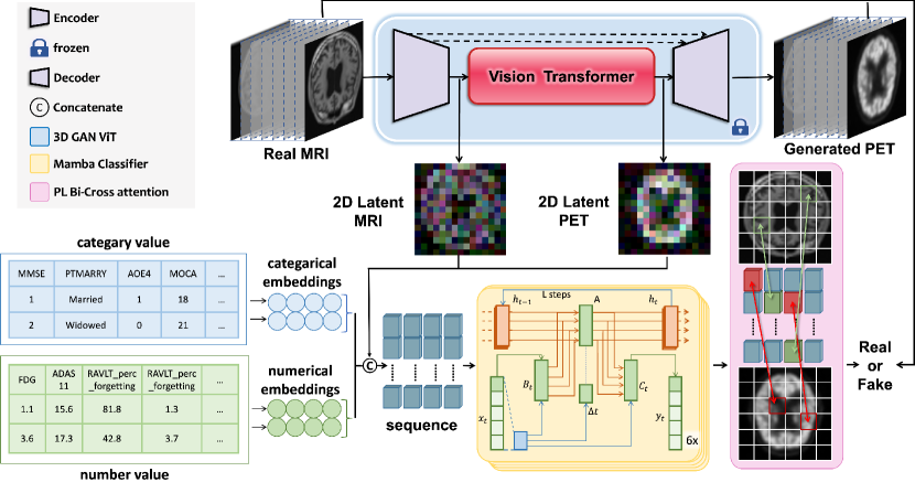
Figure 1: The overall architecture of GFE-Mamba. It contains a 3D GAN-Vit that was pre-trained on the MRI to PET generation task. 2D Latent MRI and PET extracted from the 3D GAN-Vit are fused with the scale information and fed into the Multimodal Mamba classifier, resulting in a binary classification outcome after Pixel-Level Bi-Cross Attention.

3.1 3D GAN-Vit From MRI To PET

MRI and PET provide essential structural, metabolic, and functional brain information, respectively, making both modalities crucial for predicting Alzheimer’s progression. However, incorporating both types of data into a classification network under clinical conditions presents two significant challenges. The first challenge is the requirement for paired MRI, PET, and labeled data, which is demanding and results in a scarcity of training data. This scarcity can easily lead to model overfitting. The second challenge is that in real clinical situations, patients often undergo only the less costly MRI scans and complete a few standard tests, leading to a lack of multimodal data. Despite these challenges, paired MRI and PET data are widely available. To address these issues, we propose constructing a generation network that translates MRI data into PET representations. This approach allows for effective representation learning on paired data and completes the pre-training process of the network in advance. For this generation network, we employ a 3D GAN-ViT architecture. Specifically, we use the 3D GAN network as the backbone and replace the original ResNet middle block with a ViT, enhancing the network’s ability to generate accurate PET representations from MRI data.

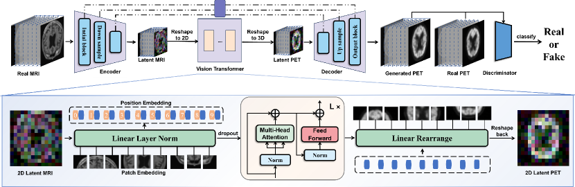
Figure 2: The architecture of 3D GAN-Vit. It consists of an Encoder, a Decoder, and a VIT as the middle layer, where the generated PET will be sent together with the real PET into the Discriminator to assess the quality of generation and training.

3.1.1 3D Generative Adversarial Network

Ian et al. proposed a Generative Adversarial Network (GAN) [2] for generating high-quality images, which can be effectively utilized in downstream tasks. The 3D GAN [3] network extends the original GAN model to three-dimensional medical scenarios. We use this 3D GAN as the backbone for our generation network. The GAN network comprises two components: a Discriminator (D) and a Generator (G). The Discriminator drives the Generator to create realistic PET images and to learn how to extract features from MRIs and transform them into PET features across extensive datasets. Consequently, even when only MRI data is available, features from both modalities can still be utilized.

The structure of our proposed 3D GAN-ViT network is illustrated in Figure 2. It consists of an Encoder/Decoder module with convolutional layers as the base, and ViT layers in the middle. The Encoder includes three down-sample modules, each comprising a max pooling layer, group normalization layer, convolutional layer, and ReLU activation layer. The channel sizes for these modules are 64, 128, and 256, respectively. The Decoder also includes three up-sample modules with channel sizes of 256, 128, and 64. Each up-sample module consists of a group normalization layer, a transpose convolutional layer, and a ReLU activation layer, mirroring the structure of the down-sample modules. The MRI input ($x_{M}$) is fed into the Generator, passing through the encoder and decoder to generate the PET output ($y_{P}$), which is then used as input for the Discriminator. The Discriminator employs the same three down-sample modules to process the input PET data ($X_{PET}$) and generates a feature map ($Y$), which participates in the loss computation.

The loss function for the 3D GAN network is divided into two parts: Generator loss and Discriminator loss. The Generator loss is defined as:

$$\mathcal{L}(G)= \sum_{x_{M}\in X_{M},y_{P}\in Y_{P}}\|G(x_{M})-y_{P}\|_{2}$$ (1)

$$+\log(1-D(G(x_{M})))+\|VGG(x_{M})-VGG(y_{P})\|_{2},$$

where the first term represents the Mean Squared Error (MSE) reconstruction loss between the real and generated PET images, the second term represents the adversarial loss of the generator, and the third term represents the perceptual loss extracted through VGG19 [28]. The Discriminator loss is defined as:

$$\mathcal{L}(D)=\sum_{x_{M}\in X_{M},y_{P}\in Y_{P}}\log(1-D(y_{P}))+\log(D(G(x_{M}))),$$ (2)

where the first term represents the adversarial loss of the discriminator on real PET images, and the second term represents the adversarial loss on the generated PET images.

3.1.2 Vision Transformer as Middle Block

The Encoder and Decoder of the 3D GAN-ViT network play crucial roles in compressing MRI data into a latent space and reconstructing it into PET data, respectively. To enhance this process, we replace the original middle block of the 3D GAN with a ViT module, rather than using the ResNet module. This change is essential because the backbone of our classifier processes sequences, and incorporating spatial features directly into this network would result in a loss of spatial information. The ViT addresses this issue by applying inter-attention to the flattened vectors of the image in the hidden space. After the Encoder extracts the MRI data into the latent space, denoted as $x_{LM}\in\mathbb{R}^{H\times W\times D\times C}$, the 3D feature map is flattened into a 2D feature map, resulting in $x_{LM}\in\mathbb{R}^{(H\cdot\sqrt{D})\times(W\cdot\sqrt{D})\times C}$. This 2D feature map is then processed by the ViT. The feature map is split into a series of image patch sequences $x_{LMP}\in\mathbb{R}^{N\times(p^{2}\cdot C)}$ through Patch Embedding, where $p$ is the patch size and $N$ is $\frac{(H\cdot\sqrt{D})}{p}$. Once the 3D feature map is transformed into a sequence, it is passed through the transformer encoder, which comprises four transformer blocks. After processing, the sequence $x_{LMP}\in\mathbb{R}^{N\times(p^{2}\cdot C)}$ is resized back to $x_{LP}\in\mathbb{R}^{H\times W\times D\times C}$ and used by the Decoder to generate the PET image. Upon pre-training, the latent representations $x_{LMP}$ for MRI and $x_{LPP}$ for PET in the hidden space effectively capture the information from both modalities. These representations are then collected and provided to the classifier for the next phase of information fusion.

3.2 Multimodal Mamba Classifier

3.2.1 Time Interval Extraction

To predict the progression from MCI to AD, the first step is to determine the prediction time interval, such as whether a patient with MCI will transition to AD within a specific period, like 180 days. For instance, if a 180-day interval is chosen, the model would predict whether a patient with MCI will develop AD after 180 days. Consequently, the training set should reflect this same interval between diagnoses. However, constructing this training dataset poses a challenge since it is difficult to ensure that the time between two diagnoses for a patient is exactly 180 days. To address this, we implement a dynamic strategy. We record the actual time intervals between diagnoses for each patient and incorporate this information into the model’s training data, along with the assessment scale category values. During inference, we use the average value of the time intervals from the training set to make predictions. This approach compensates for variations in the exact timing of patient diagnoses and ensures that the model can effectively predict the progression from MCI to AD within the specified time frame.

3.2.2 Preprocessing of Assessment Scales

To enhance the predictive accuracy of our model, we also incorporate assessment scales, similar to how physicians reference both MRI and PET images alongside diagnostic scales. Integrating these scales into the model serves two primary purposes: 1). The scales provide a direct diagnostic aid. 2). Information in tables is highly structured, making it less noisy compared to images. However, to achieve effective classification through multimodal fusion, it is essential to process the assessment scale information and integrate it with the image data. We begin by categorizing the scale information into discrete category values and continuous numerical values.

For the discrete category values: we first convert them into unique heat codes to ensure there is no duplication across different rows. To achieve this, the value in each subsequent column is increased by the maximum number of categories from all previous columns: $e_{i}^{cat}=e_{i}^{cat}+\sum_{j=1}^{i-1}\max(e_{j}^{cat})$. Once these new values are obtained, they can be embedded using a linear transformation:

$$T_{i}^{cat}=W_{i}^{cat}e_{i}^{cat}+b_{i}^{cat},$$ (3)

where $b_{i}^{cat}$ represents the bias for the $i$-th feature, and $W_{i}^{cat}$ is the look-up table for the $i$-th category [9].

For the continuous number values: this involves calculating the mean ($\mu_{i}^{num}$) and standard deviation ($\sigma_{i}^{num}$) for each column, then normalizing the values as follows: $x_{i}^{num}=(x_{i}^{num}-\mu_{i}^{num})\/\sigma_{i}^{num}$. These normalized values are then embedded using a linear transformation:

$$T_{i}^{num}=W_{i}^{num}x_{i}^{num}+b_{i}^{num}.$$ (4)

After processing both categorical and numerical values, the tabular information is combined with the image features. This is expressed as:

$$x=stack[x_{LMP},x_{LPP},T]\in\mathbb{R}^{(m+n+2N)\times d},$$ (5)

where $n$ and $m$ represent the number of categorical and numerical value rows, respectively. $x_{\text{LMP}}$ and $x_{\text{LPP}}$ denote the features of MRI and PET images in the hidden space of the generative network, and $d$ is the embedding size. Once processed, $x$ is fed into the classification network, where it is fused with image information for prediction.

3.2.3 Mamba Classifier

Given that the input $x\in\mathbb{R}^{(m+n+2N)\times d}$ consists of diverse scale information and a significantly long sequence length due to the 3D image features, using a traditional transformer with quadratic attention complexity for training is inefficient. To address the challenges of modeling long sequences, we employ the Mamba Model [10]. After processing and merging the tabular information with the image information, the sequence is fed into the classifier, which consists of six Mamba blocks. The architecture of the Mamba blocks is illustrated in Figure 3 (Part A). Each Mamba block begins by normalizing the input sequence with RMS Normalization, which calculates the root mean square value of the input activations, effectively preventing gradient explosion in deep networks.

The Mamba module then processes the input sequence, and the output is summed with the residuals of the inputs:

$$x_{i+1}=\text{Mamba}(\text{RMSNorm}(x_{i}))+x_{i}.$$

The input features are first passed through a linear layer and then split into two parts: $x$ and $z$, where $x,z=\text{split}(\text{linear}(x))$. The $x$ part is passed through a 1D convolution, followed by activation and further processing by the Selective Scan Model (SSM):

$$y=\text{SSM}(\text{Conv}(x)).$$

Meanwhile, the $z$ part functions as a gate vector and is element-wise multiplied with $y$ after activation. After the Mamba classifier, $y$ is passed through a linear layer to produce the final result of this module. Subsequently, the output passes through the Pixel-Level Bi-Cross Attention module and another linear layer to yield the final binary classification result:

$$y_{cls}=linear(Crossatten(mean(y),x_{M},x_{P}))\in\mathbb{R}^{2}.$$ (6)

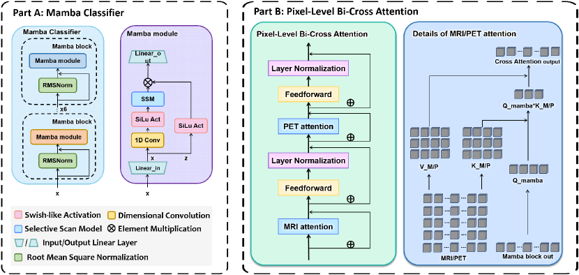
Figure 3: Part A is details of Mamba Classifier and the Mamba module in it. Part B is details of Pixel-Level Bi-Cross Attention module.

3.3 Pixel Level Bi-Cross Attention

The classifier integrates image features from MRI and PET with tabular data during forward propagation. However, it does not effectively utilize the pixel-level information from these images. Directly converting 3D MRI/PET data into sequences for the classifier results in long sequence lengths, which slow down the training process. Furthermore, the concatenation of extensive image information can prevent the classifier from effectively incorporating scale information. To address this issue, the Cross Attention architecture [29] can be employed. This method does not incorporate the forward propagation of the classifier but makes the pixel space information from MRI and PET available to the sequences in the classifier through attention mechanisms. As illustrated in Fig 3 (Part B), the output from the last Mamba block in the classifier, denoted as $y\in\mathbb{R}^{1\times d}$, is enhanced through mutual attention with MRI and PET before the final classification.

For the MRI and PET data, represented as $x_{M}$ and $x_{P}\in\mathbb{R}^{H\times W\times D\times C}$, the data are reshaped to $x_{M}$ and $x_{P}\in\mathbb{R}^{(H\cdot W\cdot D)\times C}$, which is a summarized form. For MRI, the inter-attention process is as follows:

$$Q_{y}=W_{q}y,K_{x}=W_{k}x_{M},V_{x}=W_{v}x_{M},$$ (7)

$$y=softmax(\frac{Q_{y}K_{x}}{\sqrt{d_{k}}})V_{x},$$ (8)

where the query matrix ($Q_{y}$) is derived by linearly transforming the classifier’s output, and both the key ($K_{x}$) and value matrices ($V_{x}$) are obtained by linearly transforming the serialized MRI features. This mutual attention process is similarly applied to the PET data.

After computing the mutual attention, these features are combined residually with $y$. Following the feed-forward and layer normalization operations, they are again residually summed with the original $y$.

4 Experiment

4.1 Data Acquisition and Processing

To validate our approach, we implemented it using the publicly available ADNI dataset. As outlined in this paper, our model training requires two distinct datasets: the paired MRI and PET dataset, referred to as the MRI-PET dataset, and the dataset used to determine if a classifier predicts progression to AD, referred to as the MCI-AD dataset. Due to ADNI’s privacy policy, we are unable to publicly share the screened and processed datasets. However, we will provide a detailed description of the construction of these two datasets.

4.1.1 MRI-PET Dataset

The dataset constraints are relatively flexible, requiring corresponding MRI and PET scans taken from the same patient at the same diagnostic stage. This dataset needs to be substantial in size to train on a generative network and undergo representation learning effectively. During our data collection process, we traversed through ADNI1, ADNI2, ADNI3, ADNI4, and ADNI-GO datasets. According to existing literature, specifically [2, 3], MRI and PET scans taken within ten days of each other are considered representative of the patient’s state at that moment. For image protocols, we selected the Sagittal phase, 3D, T1-weighted MRI scans without preprocessing (MPRAGE). For PET scans, we chose 18F-FDG and applied the following preprocessing steps: co-registration, averaging and standard normalization of image and voxel sizes, and uniform resolution adjustment. Our collection efforts yielded 2,843 paired MRI and PET datasets. These were divided into 2,274 pairs for the training set and 569 pairs for the validation set. The 3D images, initially in DICOM format, were converted to NIfTI format using MRIcron for easier data handling.

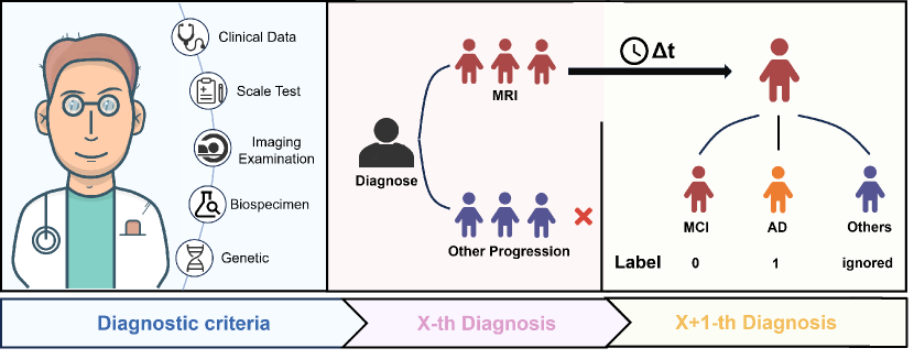
Figure 4: The process of constructing MCI-AD dataset from ADNI dataset.

4.1.2 MCI-AD Dataset

To construct the dataset for this task, it was essential to determine each patient’s status at each diagnosis. We utilized the tadpole table data from ADNI’s study data, which details the basic and pathological information of each patient. Initially, we identified all patients diagnosed with MCI and then tracked their subsequent diagnoses longitudinally. We recorded the status and timing of each following diagnosis, as illustrated in Figure 4. If a patient’s subsequent diagnosis was AD, the classification label was set to 1, otherwise, it was set to 0.

Following the label construction, we identified the corresponding MRI images based on the form information. We searched for and downloaded the relevant MRIs from the ADNI image dataset using the patient’s ID and consultation time recorded in the table. The MRI data, initially in DICOM format, was then converted to NIfTI format.

We also modified the tadpole table by adding a column for the time interval between diagnoses, denoted as $\Delta t$, and removed unnecessary information. The deletions included: 1) redundant data like the subset it belongs to (e.g., ADNI1), 2) hints with labeled information like diagnosis results, and 3) complex metrics, such as the volume of specific brain regions, which were not relevant for clinical diagnosis and training scenarios. The average time interval between diagnoses was approximately 6.7 months, excluding extreme values (e.g., $\Delta t\leq 150$).

After processing, we obtained two datasets: a one-year progression dataset and a three-year progression dataset. The one-year dataset contains 302 samples, divided into 242/60 for training/testing. The three-year dataset contains 351 samples, divided into 281/70 for training/testing. The MCI-AD dataset comprises 136 positive samples and 155 negative samples. These datasets correspond to intervals of $150\leq\Delta t\leq 365$ days and $365\leq\Delta t\leq 1095$ days, respectively. Table 1 shows the mean, variance, and the number of positive and negative samples for $\Delta t$ in these datasets.

Table 1: MVoPS/MVoNS: Mean Value of Positive/Negative Samples, SDoPS/SDoNS: Standard Deviation of Positive/Negative Samples, PS/NS: the ratio of Positive/Negative Samples.

Dataset	MvoPS	MVoNS	SDoPS	SDoNS	PS/NS
$150<\Delta t<365$	6.7	7.26	1.65	2.32	134/168
$365<\Delta t<1095$	9.06	9.57	5.21	6.27	163/218

4.2 Experimental Settings

Both components were conducted using the PyTorch 2.0 framework on NVIDIA GeForce RTX 4090 GPUs with CUDA 11.8. For reading NIfTI format images, we employed Monai, while Pandas was used to read tables and convert them into training data. The 3D GAN-ViT model was trained for 200 epochs with a batch size of 2. The classifier was trained for 100 epochs with a batch size of 8. Both models were optimized using the Adam algorithm, with a learning rate and betas set to (0.9, 0.999).

4.3 Evaluation Indicators

We employed five metrics to evaluate the classification performance on the dataset derived from ADNI: Accuracy, Precision, Recall, F1-score, and Matthews Correlation Coefficient (MCC). Their definitions and formulas are as follows:

$$Precision=\frac{TP}{TP+FP},$$ (9)

$$Recall=\frac{TP}{TP+FN},$$ (10)

$$F1-score=2\times\frac{Precision\times Recall}{Precision+Recall},$$ (11)

$$Accuracy=\frac{TP+TN}{TP+TN+FP+FN},$$ (12)

$$MCC=\frac{TP\times TN-FP\times FN}{\sqrt{(TP+FP)(TP+FN)(TN+FP)(TN+FN)}},$$ (13)

where $TP$ and $TN$ represent correctly predicted positive and negative samples, respectively, while $FP$ and $FN$ represent incorrectly predicted positive and negative samples.

4.4 Comparative Experiments

As shown in Tables 2 and 3, we compared our GFE-Mamba model with other typical classification models and advanced AD prediction models using the ADNI dataset. The results indicate that GFE-Mamba significantly outperforms these models, particularly in terms of MCC and Accuracy. Given the consistency of our findings across both datasets, we will focus on the comparative analysis using the 1-year dataset.

Table 2: Comparison of GFE-Mamba with other state-of-the-art models in 1-year Dataset.

Method	Precision	Recall	F1-score	Accuracy	MCC
Resnet50 [30]	81.03%	78.95%	68.18%	73.17%	59.00%
Resnet101 [30]	79.31%	47.37%	81.82%	60.00%	50.57%
TabTransformer [31]	84.29%	93.33%	75.68%	83.58%	70.22%
XGBoost [32]	88.14%	86.53%	86.92%	87.37%	73.90%
Qiu et al’s [33]	86.67%	81.82%	81.82%	81.82%	71.29%
Fusion model [34]	89.83%	88.21%	88.91%	89.87%	78.06%
Zhang et al’s [35]	76.67%	83.33%	45.45%	58.82%	48.42%
GFE-Mamba(Ours)	95.71%	93.33%	96.55%	94.92%	91.25%

In comparison to the ResNet family of models [30], which address gradient vanishing in deep networks, GFE-Mamba exhibits superior performance in handling MRI images. While ResNet models struggle to capture localized pathology, GFE-Mamba leverages the 3D GAN-ViT module to effectively process spatial vectors and capture spatial information, thereby improving classification accuracy. Specifically, the ResNet50 model lags behind GFE-Mamba in Precision and Accuracy, achieving only 79.31% and 60.00%, respectively.

Similarly, compared to the TabTransformer model [31], which excels in tabular data processing, GFE-Mamba demonstrates a stronger ability to capture pathological features in MRI images and recognize complex pathological states. By integrating the 3D GAN-ViT module and the Multimodal Mamba Classifier, GFE-Mamba significantly enhances classification accuracy and model interpretability. The TabTransformer model’s Recall and F1-score are notably lower, at 93.33% and 75.68%, respectively.

When compared with traditional AD classification models such as XGBoost [32] and Qiu et al’s [33], it well solves the problem of limited feature extraction capability and parameter redundancy caused by the first paper’s model relying on traditional CNN. Meanwhile, our GFE-Mamba model compensates well for the problem of high computational complexity and insufficient global information capture of 3D CNN models when dealing with high-dimensional neuroimaging data by introducing a Pixel-Level Bi-Cross Attention mechanism. As a result, GFE-Mamba is significantly improved regarding feature expression capability and model interpretability. In contrast, the Early-Stage Alzheimer’s model and 3D CNN model did not perform as well as GFE-Mamba on Recall and F1-score, which were 86.53%, 86.92%, and 81.82%, 81.82%, respectively.

Furthermore, when compared to advanced AD classification models like the Fusion model [34] and Zhang et al.’s model [35], GFE-Mamba demonstrates superior performance. While these models perform well in multimodal data processing and feature extraction, they struggle with feature redundancy and nonlinear feature representation, particularly in complex neuroimaging data. GFE-Mamba addresses these issues by combining the 3D GAN-ViT and Multimodal Mamba Classifier, thereby reducing spatial and channel redundancy and optimizing feature representation. The Pixel-Level Bi-Cross Attention mechanism further enhances nonlinear feature representation and model interpretability, while also reducing memory consumption and computational complexity. Consequently, GFE-Mamba excels in capturing fine-grained MRI features and accurately differentiating complex pathological states. In contrast, the Multimodal deep learning model and AD classification model deliver lower Precision and F1-score, with values of 89.83%, 88.91%, and 76.67%, 45.45%, respectively.

Table 3: Comparison of GFE-Mamba with other state-of-the-art models in 3-year Dataset.

Method	Precision	Recall	F1-score	Accuracy	MCC
Resnet50 [30]	77.59%	75.00%	65.22%	69.77%	52.42%
Resnet101 [30]	77.14%	73.33%	73.33%	73.33%	53.33%
TabTransformer [31]	82.86%	63.33%	95.00%	76.00%	66.64%
XGBoost [32]	90.00%	89.95%	89.75%	89.58%	79.53%
Qiu et al’s [33]	82.35%	84.62%	73.33%	78.57%	64.17%
Fusion model [34]	91.43%	91.25%	91.25%	91.25%	82.50%
Zhang et al’s [35]	70.59%	60.87%	93.33%	73.68%	48.79%
GFE-Mamba(Ours)	94.83%	94.74%	90.00%	92.31%	88.48%

4.5 Ablation Experiments

In the ablation experiments section, we analyze the individual contributions of the GFE, Cross Attention, and ViT middle block components to the classification performance of the GFE-Mamba model on the 1-year and 3-year datasets. We evaluated the impact of each module by comparing the Accuracy, Precision, Recall, F1-score, and MCC values when removing the GFE module, the Cross Attention module, and the ViT middle block module, as well as using the complete GFE-Mamba model. Tables 4 and 5 present the results, demonstrating that each module positively impacts the model’s classification performance. Given the consistency of the results across both datasets, we will focus our discussion on the ablation experiments conducted on the 1-year dataset.

Table 4: Ablation Experiments of GFE-Mamba on 1-year Dataset.

Method	Precision	Recall	F1-score	Accuracy	MCC
w/o Generative Feature Extraction	88.57%	83.33%	89.29%	86.21%	76.60%
w/o Bi-Cross Attention	92.86%	90.00%	93.10%	91.53%	85.39%
w/o Vit Middle Block	91.38%	85.00%	89.47%	87.18%	82.14%
w/o Image Data	89.66%	78.95%	88.24%	83.33%	76.11%
w/o Table Data	86.21%	68.42%	86.67%	76.47%	67.84%
GFE-Mamba(Ours)	95.71%	93.33%	96.55%	94.92%	91.25%

Impact of Removing Generative Feature Extraction: The GFE module enhances the model’s ability to extract features from high-dimensional neuroimaging data using GANs. Removing this module significantly limits the model’s feature extraction capability, resulting in a notable decline in performance. Specifically, Precision drops from 95.71% to 88.57%, and the F1-score decreases from 96.55% to 89.29%. This underscores the critical role of the GFE module in optimizing feature representation, particularly for capturing fine-grained features in MRI data.

Impact of Removing Bi-Cross Attention Module: The Bi-Cross Attention module enhances the model’s ability to capture correlations between different data modalities, thereby improving feature representation and model interpretability. Removing this module significantly weakens the model’s capacity to integrate multimodal data, leading to a marked decline in performance metrics. Specifically, Recall decreases from 96.55% to 93.10%, and the MCC drops from 91.25% to 91.53%. These results highlight the importance of the Bi-Cross Attention mechanism in accurately extracting and integrating information from multimodal data for comprehensive understanding and precise classification of complex pathological features.

Impact of Removing ViT Middle Block: The middle block enhances the model’s ability to capture global spatial information through the ViT, allowing the model to handle a wide range of spatial relationships and subtle features in MRI images. Removing this block reduces the model’s capability to capture global spatial features, leading to decreased performance. Specifically, Accuracy drops from 95.71% to 87.18%, and Recall falls from 96.55% to 89.47%. The diminished ability to extract global features makes it challenging for the model to effectively distinguish complex pathologies. This emphasizes the critical role of the ViT middle block in capturing global spatial features, which is essential for identifying complex pathological states.

Impact of Removing Image Data: Image data plays a crucial role in the model’s overall performance. Without image data, the model’s ability to extract features is significantly diminished, impacting its accuracy in recognizing pathological states. The absence of visual cues hampers efficient classification, leading to a notable decline in performance metrics. Specifically, Precision drops from 93.33% to 78.95%, and MCC falls from 91.25% to 83.33%. These results underscore the importance of image data in capturing essential pathological features for accurate diagnosis.

Impact of Removing Tabular Data: Tabular data plays a crucial role in multimodal data fusion. When tabular data is removed, the model’s ability to integrate information from multiple sources diminishes, impairing its comprehensive understanding of pathological features. The absence of tabular data hinders the model’s effectiveness in utilizing multi-source information, resulting in a significant drop in performance metrics. Specifically, Accuracy declines from 95.71% to 76.47%, and the F1-score decreases from 96.55% to 86.67%. These findings highlight the importance of tabular data in complementing image data for accurate and effective classification.

Table 5: Ablation Experiments of GFE-Mamba on 3-year Dataset.

Method	Precision	Recall	F1-score	Accuracy	MCC
w/o Generative Feature Extraction	86.21%	65.00%	92.86%	76.47%	69.28%
w/o Bi-Cross Attention	91.43%	83.33%	96.15%	89.29%	82.79%
w/o Vit Middle Block	90.00%	86.67%	89.66%	88.14%	79.53%
w/o Image Data	87.93%	75.00%	88.24%	81.08%	72.82%
w/o Table Data	84.48%	75.00%	78.95%	76.92%	65.30%
GFE-Mamba(Ours)	94.83%	94.74%	90.00%	92.31%	88.48%

5 Conclusion

The GFE-Mamba model presented in this paper addresses the challenges of multimodal data fusion, feature expressiveness, and model interpretability in predicting the progression from MCI to AD. By integrating a 3D GAN-Vit model, a Multimodal Mamba Classifier, and a Pixel-Level Bi-Cross Attention mechanism, the GFE-Mamba effectively extracts pathological features from MRI images, incorporating scale information for robust fusion. This robustness in AD classification is maintained even in scenarios with incomplete data.

The effectiveness and robustness of the GFE-Mamba model is validated through comparative and ablation experiments using the ADNI dataset. Our model significantly outperforms other state-of-the-art models across multiple performance metrics. In addition, the ablation studies demonstrate that removing any module component results in a substantial decrease in model performance, underscoring the importance of each component in fully extracting and utilizing multimodal data, thereby enhancing classification accuracy.

References

- [1] G. Livingston, J. Huntley, A. Sommerlad, D. Ames, C. Ballard, S. Banerjee, C. Brayne, A. Burns, J. Cohen-Mansfield, C. Cooper, et al., Dementia prevention, intervention, and care: 2020 report of the lancet commission, The lancet 396 (10248) (2020) 413–446.
- [2] J. Jia, F. Wang, C. Wei, A. Zhou, X. Jia, F. Li, M. Tang, L. Chu, Y. Zhou, C. Zhou, et al., The prevalence of dementia in urban and rural areas of china, Alzheimer’s & dementia 10 (1) (2014) 1–9.
- [3] C. R. Jack Jr, D. A. Bennett, K. Blennow, M. C. Carrillo, B. Dunn, S. B. Haeberlein, D. M. Holtzman, W. Jagust, F. Jessen, J. Karlawish, et al., Nia-aa research framework: toward a biological definition of alzheimer’s disease, Alzheimer’s & dementia 14 (4) (2018) 535–562.
- [4] N. Mattsson-Carlgren, S. Janelidze, S. Palmqvist, N. Cullen, A. L. Svenningsson, O. Strandberg, D. Mengel, D. M. Walsh, E. Stomrud, J. L. Dage, et al., Longitudinal plasma p-tau217 is increased in early stages of alzheimer’s disease, Brain 143 (11) (2020) 3234–3241.
- [5] J. Cummings, The role of biomarkers in alzheimer’s disease drug development, Reviews on Biomarker Studies in Psychiatric and Neurodegenerative Disorders (2019) 29–61.
- [6] M. F. Folstein, S. E. Folstein, P. R. McHugh, “mini-mental state”: a practical method for grading the cognitive state of patients for the clinician, Journal of psychiatric research 12 (3) (1975) 189–198.
- [7] Z. S. Nasreddine, N. A. Phillips, V. Bédirian, S. Charbonneau, V. Whitehead, I. Collin, J. L. Cummings, H. Chertkow, The montreal cognitive assessment, moca: a brief screening tool for mild cognitive impairment, Journal of the American Geriatrics Society 53 (4) (2005) 695–699.
- [8] L. C. Clark Jr, C. Lyons, Electrode systems for continuous monitoring in cardiovascular surgery, Annals of the New York Academy of sciences 102 (1) (1962) 29–45.
- [9] R. C. Petersen, P. Aisen, B. F. Boeve, Y. E. Geda, R. J. Ivnik, D. S. Knopman, M. Mielke, V. S. Pankratz, R. Roberts, W. A. Rocca, et al., Mild cognitive impairment due to alzheimer disease in the community, Annals of neurology 74 (2) (2013) 199–208.
- [10] H. Hampel, S. E. O’Bryant, J. L. Molinuevo, H. Zetterberg, C. L. Masters, S. Lista, S. J. Kiddle, R. Batrla, K. Blennow, Blood-based biomarkers for alzheimer disease: mapping the road to the clinic, Nature Reviews Neurology 14 (11) (2018) 639–652.
- [11] J. Escudero, J. P. Zajicek, E. Ifeachor, Early detection and characterization of alzheimer’s disease in clinical scenarios using bioprofile concepts and k-means, in: 2011 Annual International Conference of the IEEE Engineering in Medicine and Biology Society, IEEE, 2011, pp. 6470–6473.
- [12] C. Misra, Y. Fan, C. Davatzikos, Baseline and longitudinal patterns of brain atrophy in mci patients, and their use in prediction of short-term conversion to ad: results from adni, Neuroimage 44 (4) (2009) 1415–1422.
- [13] J. Ye, M. Farnum, E. Yang, R. Verbeeck, V. Lobanov, N. Raghavan, G. Novak, A. DiBernardo, V. A. Narayan, A. D. N. Initiative, Sparse learning and stability selection for predicting mci to ad conversion using baseline adni data, BMC neurology 12 (2012) 1–12.
- [14] J. Wan, Z. Zhang, J. Yan, T. Li, B. D. Rao, S. Fang, S. Kim, S. L. Risacher, A. J. Saykin, L. Shen, Sparse bayesian multi-task learning for predicting cognitive outcomes from neuroimaging measures in alzheimer’s disease, in: 2012 IEEE Conference on Computer Vision and Pattern Recognition, IEEE, 2012, pp. 940–947.
- [15] J. Young, M. Modat, M. J. Cardoso, A. Mendelson, D. Cash, S. Ourselin, A. D. N. Initiative, et al., Accurate multimodal probabilistic prediction of conversion to alzheimer’s disease in patients with mild cognitive impairment, NeuroImage: Clinical 2 (2013) 735–745.
- [16] C. Plant, S. J. Teipel, A. Oswald, C. Böhm, T. Meindl, J. Mourao-Miranda, A. W. Bokde, H. Hampel, M. Ewers, Automated detection of brain atrophy patterns based on mri for the prediction of alzheimer’s disease, Neuroimage 50 (1) (2010) 162–174.
- [17] S. J. Teipel, C. Born, M. Ewers, A. L. Bokde, M. F. Reiser, H.-J. Möller, H. Hampel, Multivariate deformation-based analysis of brain atrophy to predict alzheimer’s disease in mild cognitive impairment, Neuroimage 38 (1) (2007) 13–24.
- [18] E. Moradi, A. Pepe, C. Gaser, H. Huttunen, J. Tohka, A. D. N. Initiative, et al., Machine learning framework for early mri-based alzheimer’s conversion prediction in mci subjects, Neuroimage 104 (2015) 398–412.
- [19] A. Elazab, C. Wang, M. Abdelaziz, J. Zhang, J. Gu, J. M. Gorriz, Y. Zhang, C. Chang, Alzheimer’s disease diagnosis from single and multimodal data using machine and deep learning models: Achievements and future directions, Expert Systems with Applications (2024) 124780.
- [20] C. Liu, F. Huang, A. Qiu, A. D. N. Initiative, et al., Monte carlo ensemble neural network for the diagnosis of alzheimer’s disease, Neural Networks 159 (2023) 14–24.
- [21] S. Qiu, P. S. Joshi, M. I. Miller, C. Xue, X. Zhou, C. Karjadi, G. H. Chang, A. S. Joshi, B. Dwyer, S. Zhu, et al., Development and validation of an interpretable deep learning framework for alzheimer’s disease classification, Brain 143 (6) (2020) 1920–1933.
- [22] L. Liu, S. Liu, L. Zhang, X. V. To, F. Nasrallah, S. S. Chandra, Cascaded multi-modal mixing transformers for alzheimer’s disease classification with incomplete data, NeuroImage 277 (2023) 120267.
- [23] N. Rahim, S. El-Sappagh, S. Ali, K. Muhammad, J. Del Ser, T. Abuhmed, Prediction of alzheimer’s progression based on multimodal deep-learning-based fusion and visual explainability of time-series data, Information Fusion 92 (2023) 363–388.
- [24] S. El-Sappagh, T. Abuhmed, S. R. Islam, K. S. Kwak, Multimodal multitask deep learning model for alzheimer’s disease progression detection based on time series data, Neurocomputing 412 (2020) 197–215.
- [25] M. Wang, W. Shao, S. Huang, D. Zhang, Hypergraph-regularized multimodal learning by graph diffusion for imaging genetics based alzheimer’s disease diagnosis, Medical Image Analysis 89 (2023) 102883.
- [26] D. Zeng, S. Chen, B. Chen, S. Li, Improving remote sensing scene classification by integrating global-context and local-object features, Remote Sensing 10 (5) (2018) 734.
- [27] S. Ge, C. Li, S. Zhao, D. Zeng, Occluded face recognition in the wild by identity-diversity inpainting, IEEE Transactions on Circuits and Systems for Video Technology 30 (10) (2020) 3387–3397.
- [28] R. A. Nebel, N. T. Aggarwal, L. L. Barnes, A. Gallagher, J. M. Goldstein, K. Kantarci, M. P. Mallampalli, E. C. Mormino, L. Scott, W. H. Yu, et al., Understanding the impact of sex and gender in alzheimer’s disease: a call to action, Alzheimer’s & Dementia 14 (9) (2018) 1171–1183.
- [29] E. M. Arenaza-Urquijo, P. Vemuri, Resistance vs resilience to alzheimer disease: clarifying terminology for preclinical studies, Neurology 90 (15) (2018) 695–703.
- [30] K. He, X. Zhang, S. Ren, J. Sun, Deep residual learning for image recognition, in: Proceedings of the IEEE conference on computer vision and pattern recognition, 2016, pp. 770–778.
- [31] X. Huang, A. Khetan, M. Cvitkovic, Z. Karnin, Tabtransformer: Tabular data modeling using contextual embeddings, arXiv preprint arXiv:2012.06678 (2020).
- [32] C. Kavitha, V. Mani, S. Srividhya, O. I. Khalaf, C. A. Tavera Romero, Early-stage alzheimer’s disease prediction using machine learning models, Frontiers in public health 10 (2022) 853294.
- [33] S. Qiu, P. S. Joshi, M. I. Miller, C. Xue, X. Zhou, C. Karjadi, G. H. Chang, A. S. Joshi, B. Dwyer, S. Zhu, et al., Development and validation of an interpretable deep learning framework for alzheimer’s disease classification, Brain 143 (6) (2020) 1920–1933.
- [34] S. Qiu, M. I. Miller, P. S. Joshi, J. C. Lee, C. Xue, Y. Ni, Y. Wang, I. De Anda-Duran, P. H. Hwang, J. A. Cramer, et al., Multimodal deep learning for alzheimer’s disease dementia assessment, Nature communications 13 (1) (2022) 3404.
- [35] Y. ZHANG, X. WU, L. TANG, Q. XU, B. WANG, X. HE, Alzheimer’s disease classification method based on multimodal data, Journal of Computer Applications 43 (S2) (2023) 298.