Distributions of consecutive level spacings of GUE and their ratio: an analytic treatment

\name\fnameShinsuke \surnameM. Nishigaki   nishigaki@riko.shimane-u.ac.jp Graduate School of Natural Science and Technology, Shimane University, Matsue 690-8504, Japan
Abstract

In recent studies of many-body localization in nonintegrable quantum systems, the distribution of the ratio of two consecutive energy level spacings, $r_{n}=(E_{n+1}-E_{n})/(E_{n}-E_{n-1})$ or $\tilde{r}_{n}=\min(r_{n},r_{n}^{-1})$, has been used as a measure to quantify the chaoticity, alternative to the more conventional distribution of the level spacings, $s_{n}=\bar{\rho}(E_{n})(E_{n+1}-E_{n})$, as the former unnecessitates the unfolding required for the latter. Based on our previous work on the Tracy-Widom approach to the Jánossy densities, we present analytic expressions for the joint probability distribution of two consecutive eigenvalue spacings and the distribution of their ratio for the Gaussian unitary ensemble (GUE) of random Hermitian $N\times N$ matrices at $N\to\infty$, in terms of a system of differential equations. As a showcase of efficacy of our results for characterizing an approach to quantum chaoticity, we contrast them to arguably the most ideal of all quantum-chaotic spectra: the zeroes of the Riemann $\zeta$ function on the critical line at increasing heights.

\subjectindex

A10,A13,A32,B83,B86

1 Introduction

Many-body localization that prohibits thermal equilibration of the wave functions has been a core agenda of research in the field of quantum many-body systems, including disordered and interacting fermions on a chain Oganesyan:2007 , spin chains with transverse field, periodical kicks, or disorder Atas:2013 ; Kim:2013 ; DAlessio:2014 ; Luitz:2015 , and the Sachdev-Ye-Kitaev model and its deformed, coupled, or sparsed variant You:2017 ; Garcia:2018 ; Garcia:2019 ; Garcia:2021 , to name but the few. In all of the above studies, the ‘gap ratio distribution’, i.e. the distribution $P_{\mathrm{r}}(r)$ of ratio of consecutive energy level spacings $r_{n}=(E_{n+1}-E_{n})/(E_{n}-E_{n-1})$ or $\tilde{r}_{n}=\min(r_{n},r_{n}^{-1})$, initiated by Ref. Oganesyan:2007 , has been utilized as a criteria of (non)ergodicity. This trend is obviously due to its computational advantage that unnecessitates the unfolding by the smoothed density of states $\bar{\rho}(E)$, over the conventional distribution $P(s)$ of level spacings $s_{n}=\bar{\rho}(E_{n})(E_{n+1}-E_{n})$. More recently, the use of the gap ratio distribution for characterizing spectral transitions extended its reach beyond energy level statistics of many-body or chaotic Hamiltonians, namely towards quantum entanglement spectra of reduced density matrices in neural network states Deng:2017 and in quantum circuits Zhang:2020 ; Jian:2022 .

The random matrix theory of the gap ratio distribution was introduced in Ref. Atas:2013 and has since been quoted in practically every work in these fields including Refs. Kim:2013 ; DAlessio:2014 ; Luitz:2015 ; You:2017 ; Garcia:2018 ; Garcia:2019 ; Garcia:2021 ; Deng:2017 ; Zhang:2020 ; Jian:2022 . There, two types of approximate expressions for $P_{\mathrm{r}}(r)$ were presented: one from the Wigner-like surmise (substituting the large-$N$ limit of $N\times N$ matrices by $3\times 3$) for all three Dyson symmetry classes, $P_{\mathrm{r}}(r)\approx C_{\beta}(r+r^{2})^{\beta}/(1+r+r^{2})^{1+3\beta/2}\ (\beta=1,2,4)$, and another from the quadrature discretization of the resolvent operator $\boldsymbol{\mathit{K}}_{I}(\mathbb{I}-\boldsymbol{\mathit{K}}_{I})^{-1}$ where $\boldsymbol{\mathit{K}}_{I}$ denotes the integral operator of convolution with the sine kernel over an interval $I$ for the unitary class $\beta=2$. Although the latter approximation is known to converge to the exact value quickly as the quadrature order is increased Bornemann:2010a , the analytical expression for $P_{\mathrm{r}}(r)$ is still missing. Moreover, the Author cannot help feeling frustrated to find that every article that quotes Ref. Atas:2013 almost always refers only to the Wigner-surmised form, and calls that crude, uncontrolled approximation the ‘outcome from the random matrix theory’. In view of these, this article aims to determine analytically the joint distribution of consecutive eigenvalue spacings $P_{\mathrm{c}}(a,b)$ and the distribution of their ratio $P_{\mathrm{r}}(r)$ for the unitary class, based on our recent work Nishigaki:2021 which provided a generic prescription for determining the Jánossy density for any integrable kernel as a solution to the Tracy-Widom system of PDEs Tracy:1994c .

This article is composed of the following parts: In §2 we list several facts on the Jánossy density $J_{1}(0;I)$ for the sine kernel, i.e. the conditional probability that an interval $I$ in the spectral bulk of the GUE contains no eigenvalue except for the one at a designated locus. In §3 we follow the prescription of Tracy and Widom and show that the Jánossy density and associated distributions of consecutive eigenvalue spacings and their ratio are analytically determined as a solution to a system of ODEs. As a showcase of efficacy of our results for characterizing an approach to quantum chaoticity without using $\bar{\rho}(E)$, in §4 we contrast them to the distribution of zeroes of the Riemann $\zeta$ function on the critical line at increasing heights. Numerical data of the Jánossy density and the program for generating them are attached as Supplementary materials.

2 Jánossy density for the sine kernel

The sine kernel

$\displaystyle K(x,y)$ $\displaystyle=\frac{\sin(x-y)}{\pi(x-y)}=\frac{\sin x\cos y-\cos x\sin y}{\pi(x-y)}$ (1)

governs the determinantal point process of unfolded*** We adopt a normalization such that the mean eigenvalue spacing is $\pi$. eigenvalues or eigenphases $\{x_{i}\}$ of random Hermitian or unitary matrices of infinite rank $N\to\infty$, in the spectral bulk Mehta ; Forrester . From the very defining property of the determinantal point process that the $p$-point correlation function ${R}_{p}(x_{1},\ldots,x_{p})=\mathbb{E}[\prod_{i=1}^{p}\delta(x-x_{i})]$ is given by $\det[K(x_{i},x_{j})]_{i,j=1}^{p}$, it follows that the conditional $p$-point correlation function

$\displaystyle\tilde{R}_{p|1}(x_{1},\ldots,x_{p}|t)=\frac{\mathbb{E}[\delta(x-t)\prod_{i=1}^{p}\delta(x-x_{i})]}{\mathbb{E}[\delta(x-t)]}$ (2)

in which one of the eigenvalues is preconditioned at $x=t$ also takes a determinantal form $\det[\tilde{K}(x_{i},x_{j})]_{i,j=1}^{p}$ governed by another kernel Daley ,

$\displaystyle\tilde{K}(x,y)=K(x,y)-K(x,t)K(t,t)^{-1}K(t,y).$ (3)

In the case of the sine kernel (1), its translational invariance allows for setting $t=0$ without loss of generality, so that Nagao:1993

$\displaystyle\tilde{K}(x,y)$ $\displaystyle=\frac{1}{\pi}\left(\frac{\sin(x-y)}{x-y}-\frac{\sin x}{x}\frac{\sin y}{y}\right)=\frac{\varphi(x)\psi(y)-\psi(x)\varphi(y)}{x-y}~{},$ (4)
$\displaystyle\varphi(x)$ $\displaystyle=\frac{1}{\sqrt{\pi}}\sin x,~{}~{}\psi(x)=\frac{1}{\sqrt{\pi}}\left(\cos x-\frac{\sin x}{x}\right).$

The transformation of kernels (3) from $K$ to $\tilde{K}$ is associated with a meromorphic $\mathrm{SL}(2,\mathbb{R})$ gauge transformation Nishigaki:2021

$\displaystyle\left[\begin{array}[]{c}\varphi(x)\\ \psi(x)\end{array}\right]=\left[\begin{array}[]{cc}1&0\\ -x^{-1}&1\\ \end{array}\right]\left[\begin{array}[]{c}\pi^{-1/2}\sin x\\ \pi^{-1/2}\cos x\end{array}\right]$ (11)

on the two-component functions that consist respective kernels in the right hand sides of (1) and (4). Accordingly, as stated in Theorem in Ref. Nishigaki:2021 , the gauge-transformed section $[\varphi(x),\psi(x)]^{T}$ inherits from the original section $[\pi^{-1/2}\sin(x),\pi^{-1/2}\cos(x)]^{T}$ the covariant-constancy condition for a meromorphic $\mathfrak{sl}(2,\mathbb{R})$ connection, i.e. a pair of linear differential equations,

$\displaystyle m(x)\frac{d}{dx}\left[\!\begin{array}[]{c}\varphi(x)\\ \psi(x)\end{array}\!\right]=\left[\!\begin{array}[]{rr}A(x)\!&\!\!B(x)\\ -C(x)\!&\!\!-A(x)\end{array}\!\right]\left[\!\begin{array}[]{c}\varphi(x)\\ \psi(x)\end{array}\!\right]\,\mbox{with polynomials}~{}m(x),A(x),B(x),C(x),$ (18)

which guarantees applicability of the Tracy-Widom method. In the present case of spherical Bessel functions (4), polynomials consisting the connection (Lax operator) $\frac{1}{m}\left[{~{}A~{}~{}B\atop-C\,-A}\right]$ are:

$\displaystyle A(x)=1,~{}~{}B(x)=C(x)=m(x)=x.$ (19)

Subsequently we shall use their nonzero coefficients,

$\displaystyle\alpha_{0}=\beta_{1}=\gamma_{1}=\mu_{1}=1.$ (20)

We take an interval $I=[a_{1},a_{2}]$ with $a_{1}<0<a_{2}$ so that the ordered triple $(a_{1},0,a_{2})$ will serve as three consecutive eigenvalues, and denote by $\tilde{\boldsymbol{\mathit{K}}}_{I}$ the integration operator acting on the Hilbert space of square-integrable functions $L^{2}(I)$ with convolution kernel $\tilde{K}(x,y)$,

$\displaystyle(\tilde{\boldsymbol{\mathit{K}}}_{I}f)(x):=\int_{I}dy\,\tilde{K}(x,y)f(y).$ (21)

Then by Gaudin and Mehta’s theorem Mehta , the Jánossy density $J_{1}(0;[a_{1},a_{2}])$ Borodin:2003 , i.e. the conditional probability that the interval $I=[a_{1},a_{2}]$ contains no eigenvalue except for the one preconditioned at $x=0$, is expressed as the Fredholm deterninant of $\tilde{\boldsymbol{\mathit{K}}}_{I}$:

$\displaystyle J_{1}(0;[a_{1},a_{2}])$ $\displaystyle=\mathrm{Det}\,(\mathbb{I}-\tilde{\boldsymbol{\mathit{K}}}_{I})=\exp\Bigl{(}-\sum_{n\geq 1}\frac{1}{n}\mathrm{Tr}\,\tilde{\boldsymbol{\mathit{K}}}_{I}^{n}\Bigr{)}$
$\displaystyle=\exp\left(-\int_{I}dx\,\tilde{K}(x,x)-\frac{1}{2}\int\!\!\!\!\int_{I}dxdy\,\tilde{K}(x,y)\tilde{K}(y,x)-\cdots\right).$ (22)

Note that the Jánossy density for a symmetric interval $I=[-t,t]$ was previously expressed in terms of a Painlevé V transcendent, i.e. a special solution to an ODE in $t$ Forrester:1996 . Our task in this article is to extend their result to a generic interval and express $J_{1}(0;[a_{1},a_{2}])$ and an associated distribution $P_{\mathrm{r}}({r})$ in terms of a system of PDEs in $a_{1}$ and $a_{2}$.

3 Tracy-Widom system

Tracy and Widom (TW) Tracy:1994c established a systematic method of computing the Fredholm determinant of an integrable integral kernel whose component functions satisfy the condition (18). The quantities that appear in the TW system [$j,k=1$ or $2$],

$\displaystyle R_{jk}$ $\displaystyle=\tilde{K}(a_{j},a_{k})+\int_{I}dx\,\tilde{K}(a_{j},x)\tilde{K}(x,a_{k})+\int\!\!\!\!\int_{I}dxdy\,\tilde{K}(a_{j},x)\tilde{K}(x,y)\tilde{K}(y,a_{k})+\cdots$
$\displaystyle=((\mathbb{I}-\tilde{\boldsymbol{\mathit{K}}}_{I})^{-1}\tilde{{K}})(a_{j},a_{k})=R_{kj},$
$\displaystyle q_{j}$ $\displaystyle=\varphi(a_{j})+\int_{I}dx\,\tilde{K}(a_{j},x)\varphi(x)+\int\!\!\!\!\int_{I}dxdy\,\tilde{K}(a_{j},x)\tilde{K}(x,y)\varphi(y)+\cdots$
$\displaystyle=((\mathbb{I}-\tilde{\boldsymbol{\mathit{K}}}_{I})^{-1}\varphi)(a_{j}),$
$\displaystyle p_{j}$ $\displaystyle=((\mathbb{I}-\tilde{\boldsymbol{\mathit{K}}}_{I})^{-1}\psi)(a_{j}),$ (23)
$\displaystyle u$ $\displaystyle=\int_{I}dx\,\varphi(x)^{2}+\int\!\!\!\!\int_{I}dxdy\,\varphi(x)\tilde{K}(x,y)\varphi(y)+\int\!\!\!\!\int\!\!\!\!\int_{I}dxdydz\,\varphi(x)\tilde{K}(x,y)\tilde{K}(y,z)\varphi(z)+\cdots$
$\displaystyle=\int_{I}dx\,\varphi(x)((\mathbb{I}-\tilde{\boldsymbol{\mathit{K}}}_{I})^{-1}\varphi)(x),$
$\displaystyle v$ $\displaystyle=\int_{I}dx\,\psi(x)((\mathbb{I}-\tilde{\boldsymbol{\mathit{K}}}_{I})^{-1}\varphi)(x),~{}~{}w=\int_{I}dx\,\psi(x)((\mathbb{I}-\tilde{\boldsymbol{\mathit{K}}}_{I})^{-1}\psi)(x),$

are all treated as functions of the left and the right endpoints $(a_{1},a_{2})$ of the interval $I$. Expanding the definitions (22), (23) in $a_{1}$ and $a_{2}\ll 1$, the boundary conditions for these quantities read:

$\displaystyle\ln$ $\displaystyle J_{1}(0;[a_{1},a_{2}])=\frac{a_{1}^{3}-a_{2}^{3}}{9\pi}-\frac{2(a_{1}^{5}-a_{2}^{5})}{225\pi}+\cdots,$
$\displaystyle q_{j}$ $\displaystyle=\frac{a_{j}}{\sqrt{\pi}}-\frac{a_{j}^{3}}{6\sqrt{\pi}}-\frac{(a_{1}^{3}-a_{2}^{3})a_{j}}{9\pi^{3/2}}+\frac{a_{j}^{5}}{120\sqrt{\pi}}+\cdots,$ (24)
$\displaystyle p_{j}$ $\displaystyle=-\frac{a_{j}^{2}}{3\sqrt{\pi}}+\frac{a_{j}^{4}}{30\sqrt{\pi}}+\frac{(a_{1}^{4}-a_{2}^{4})a_{j}}{36\pi^{3/2}}+\cdots,$
$\displaystyle u$ $\displaystyle=-\frac{a_{1}^{3}-a_{2}^{3}}{3\pi}+\frac{a_{1}^{5}-a_{2}^{5}}{15\pi}+\cdots,~{}~{}v=\frac{a_{1}^{4}-a_{2}^{4}}{12\pi}+\cdots,~{}~{}w=-\frac{a_{1}^{5}-a_{2}^{5}}{45\pi}+\cdots,$

up to terms of $O(a_{1},a_{2})^{6}$. Substituting the coefficients (20) into the TW system of PDEs (Eqs.(2.25), (2.26), (2.31), (2.32), (2.12)-(2.18), (1.7a) of Ref.Tracy:1994c ), it takes the following form [below the pair of indices $(j,k)$ assumes either $(1,2)$ or $(2,1)$]:

$\displaystyle R_{jk}$ $\displaystyle=\frac{q_{j}p_{k}-p_{j}q_{k}}{a_{j}-a_{k}}~{},$
$\displaystyle a_{j}\frac{\partial q_{j}}{\partial a_{j}}$ $\displaystyle=Uq_{j}+(V+a_{j})p_{j}-(-1)^{k}a_{k}R_{jk}q_{k}~{},$
$\displaystyle a_{j}\frac{\partial p_{j}}{\partial a_{j}}$ $\displaystyle=-Up_{j}+(V-a_{j})q_{j}-(-1)^{k}a_{k}R_{jk}p_{k}~{},$ (25)
$\displaystyle\frac{\partial q_{j}}{\partial a_{k}}$ $\displaystyle=(-1)^{k}R_{jk}q_{k}~{},~{}~{}\frac{\partial p_{j}}{\partial a_{k}}=(-1)^{k}R_{jk}p_{k}~{},$
$\displaystyle\frac{\partial u}{\partial a_{j}}$ $\displaystyle=(-1)^{j}q_{j}^{2}~{},~{}~{}\frac{\partial v}{\partial a_{j}}=(-1)^{j}q_{j}p_{j}~{},~{}~{}\frac{\partial w}{\partial a_{j}}=(-1)^{j}p_{j}^{2}~{},$

where $U=1+u-w$ and $V=2v$. The ‘stiffness’ of the second and the third equations of (25) at $a_{j}=0$ is only superficial, because $R_{jk}$, $q_{j}$, and $p_{j}$ are of $O(a_{j})$ or higher orders in the limit $a_{j}\to 0$. We remark that the above PDEs reduce to the ODEs (Eqs. (14), (15), (17)) of Ref. Forrester:1996 and $V=0$ in the symmetric case, $|a_{1}|=a_{2}=t$. The Fredholm determinant (22) is expressed by $R_{jj}$, which is composed of $q_{j}$ and $p_{j}$ ((1.3), (1.7b) of Ref. Tracy:1994c ),

$\displaystyle(-1)^{j-1}\frac{\partial}{\partial a_{j}}\ln J_{1}(0;[a_{1},a_{2}])=R_{jj}=p_{j}\frac{\partial q_{j}}{\partial a_{j}}-q_{j}\frac{\partial p_{j}}{\partial a_{j}}~{}~{}~{}(j=1,2).$ (26)

For numerical evaluation of $J_{1}(0;[a,b])$, it is practically convenient to start from the initial condition (24) at $(\epsilon a,\epsilon b)$ with a sufficiently small $\epsilon>0$ and to integrate the TW system (25), (26) in the radial direction $\left(a_{1}(s),a_{2}(s))=(sa,sb\right)$, $\epsilon\leq s\leq 1$. The resultant system of ODEs in $s$, combined from the PDEs through $s\frac{d}{ds}=a_{1}(s)\frac{\partial}{\partial a_{1}}+a_{2}(s)\frac{\partial}{\partial a_{2}}$, reads:

$\displaystyle s\frac{d}{ds}\left[\begin{array}[]{l}q_{j}\\ p_{j}\end{array}\right]=\left[\begin{array}[]{cc}U&V+a_{j}\\ V-a_{j}&-U\end{array}\right]\left[\begin{array}[]{l}q_{j}\\ p_{j}\end{array}\right]~{},$ (33)
$\displaystyle s\frac{dU}{ds}=-a_{1}(q_{1}^{2}-p_{1}^{2})+a_{2}(q_{2}^{2}-p_{2}^{2})~{},~{}s\frac{dV}{ds}=-2a_{1}q_{1}p_{1}+2a_{2}q_{2}p_{2}~{},$
$\displaystyle s\frac{d\ln J_{1}}{ds}=a_{1}(q_{1}^{2}+p_{1}^{2})-a_{2}(q_{2}^{2}+p_{2}^{2})-(q_{1}p_{2}-p_{1}q_{2})^{2}+2U(q_{1}p_{1}-q_{2}p_{2})-V(q_{1}^{2}-p_{1}^{2}-q_{2}^{2}+p_{2}^{2}).$

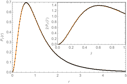
Note that the form of the first line of Eq. (33) is directly inherited from Eqs. (18), (19). It is quite plausible that the ODEs (33) can be expressible as a Hamiltonian system, and $J_{1}(0;[a_{1},a_{2}])$ be regarded as a $\tau$-function of an integrable hierarchy Forrester:2001 . However, these are not immediately evident to the Author, and will be discussed in a separate publication. As a cross-check of our formulation, we confirmed that the values of $J_{1}(0;[a_{1},a_{2}])$ obtained by the above prescription [Fig. 1, left] are identical, within the accuracy of numerical evaluation, to those from the Nyström-type quadrature approximation of the Fredholm determinant Bornemann:2010a

$\displaystyle\mathrm{Det}\,(\mathbb{I}-\tilde{\boldsymbol{\mathit{K}}}_{I})\simeq\det\left[\delta_{ij}-\tilde{K}(x_{i},x_{j})\sqrt{w_{i}w_{j}}\right]_{i,j=1}^{m}~{},$ (34)

where $\{x_{i},w_{i}\}_{i=1}^{m}$ is the $m$-th order quadrature of the interval $I$ such that $\sum_{i=1}^{m}w_{i}f(x_{i})\stackrel{{\scriptstyle m\to\infty}}{{\longrightarrow}}\int_{I}dx\,f(x)$, with a sufficiently large $m$. Specifically, relative deviations of $J_{1}(0;[a_{1},a_{2}])$ computed by the TW system (33) starting from the initial value $\epsilon=10^{-10}$ using Mathematica’s NDSolve package with WorkingPrecision$\to$ 5 MachinePrecision, and that evaluated by the Nyström-type approximation (34) with the Gauss-Legendre quadrature of order $m=200$, do not exceed $10^{-27}$ for the whole range of variables $|a_{j}|\leq 10$, and $<10^{-19}$ for $|a_{j}|\leq 20$. Interested readers are invited to verify this statement by running the Notebook Janossy_TW_N.nb included in Supplementary materials.

Refer to caption
Refer to caption
Figure 1: The Jánossy density $J_{1}(0;[a_{1},a_{2}])$ for the sine kernel [left], and the joint distribution $P_{\mathrm{c}}(a_{1},a_{2})$ of two consecutive eigenvalue spacings [right]. For visual clarity, each coordinate $a_{j}$ is rescaled from the text by $1/\pi$, so that the mean eigenvalue spacing is unity.

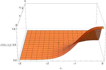
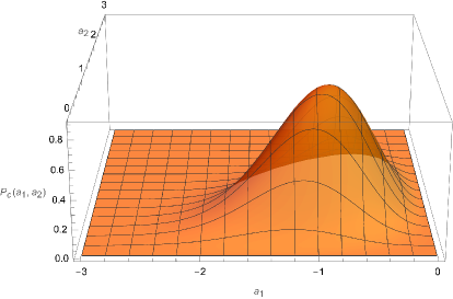
Various probability density functions follow from the Jánossy density: The level spacing distribution $P(s)$ Mehta , the distribution for the nearest neighbor level spacing $P_{\mathrm{nn}}(t)$ Forrester:1996 , and the joint distribution for the two consecutive level spacings $P_{\mathrm{c}}(a_{1},a_{2})$ Atas:2013 are given by

$\displaystyle P(s)=-\frac{dJ_{1}(0;[0,s])}{ds},\ \ P_{\mathrm{nn}}(t)$ $\displaystyle=-\frac{dJ_{1}(0;[-t,t])}{dt},\ \ P_{\mathrm{c}}(a_{1},a_{2})=-\frac{\partial^{2}J_{1}(0;[a_{1},a_{2}])}{\partial a_{1}\partial a_{2}},$ (35)

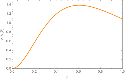
respectively [Fig. 1, right]. Finally, the distribution $P_{\mathrm{r}}(r)$ for the ratio $r=|a_{1}|/a_{2}$ of the two consecutive level spacings is given by Atas:2013 ,

$\displaystyle P_{\mathrm{r}}(r)$ $\displaystyle=\int_{0}^{\infty}da_{2}\int_{-\infty}^{0}da_{1}P_{\mathrm{c}}(a_{1},a_{2})\,\delta(r-|a_{1}|/a_{2})=\int_{0}^{\infty}da\,a\,P_{\mathrm{c}}(-ra,a)~{}.$ (36)

If we switch the variable from $r$ to $\tilde{r}:=\min(|a_{1}|,a_{2})/\max(|a_{1}|,a_{2})=\min(r,r^{-1})\in[0,1]$, its distribution is twice the above $P_{\mathrm{r}}(r)$ [Fig. 2], yielding the expectation values for its moments,

$\displaystyle\mathbb{E}[\tilde{r}^{k}]$ $\displaystyle=2\int_{0}^{\infty}da_{2}\int_{-a_{2}}^{0}da_{1}P_{\mathrm{c}}(a_{1},a_{2})\left(|a_{1}|/a_{2}\right)^{k}$ (37)
$\displaystyle=0.5997504209(1),\,0.4132049292(1),\,0.3100223500(1),\,0.2460560527(1)~{}~{}(k=1,2,3,4).$
Refer to caption
Figure 2: The distribution of the $\tilde{r}$-ratio, $\tilde{r}=\min(|a_{1}|,a_{2})/\max(|a_{1}|,a_{2})$.

4 Zeroes of the Riemann $\zeta$ function

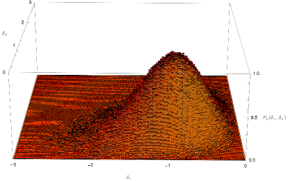
As a showcase of application of our analytic results to the judgement of quantum chaoticity, we compare them to (arguably) the most ideal of all quantum-chaotic spectra: the sequence of zeroes of the Riemann $\zeta$ function on the critical line, $\{\frac{1}{2}+i\gamma_{n}\}$. Their imaginary parts are supposed to be the eigenvalues of the hypothetical Hilbert-Pólya operator Wiki:Hilbert-Polya that should be self-adjoint, ergodic, and without any anti-unitary convolutive symmetry. After unfolding by the Riemann-von Mangoldt formula for the asymptotic density of zeroes, $\bar{\rho}(\gamma)=\frac{1}{2\pi}\log\frac{\gamma}{2\pi}$, the histogram $P_{\mathrm{c}}(\delta_{-},\delta_{+})$ of two unfolded consecutive spacings $\delta_{\pm}=\bar{\rho}(\gamma_{n})(\gamma_{n\pm 1}-\gamma_{n})$ of $10^{8}$ zeroes ending at $n=103800788359$ (the largest zero available at the LMFDB LMFDB ) perfectly agree with the GUE result (35), as visualized in Fig. 3, left. Moreover, had we not known the classical formula for $\bar{\rho}(\gamma)$ a priori, the perfect match to the GUE could still be deduced from the distributions of the ratios of consecutive spacings of zeroes $r_{n}=(\gamma_{n+1}-\gamma_{n})/(\gamma_{n}-\gamma_{n-1})$ and $\tilde{r}_{n}=\min(r_{n},r_{n}^{-1})$ [Fig. 3, right].

Refer to caption
Refer to caption
Figure 3: The joint distribution $P_{\mathrm{c}}(\delta_{-},\delta_{+})$ of two unfolded consecutive spacings $\delta_{\pm}=\bar{\rho}(\gamma_{n})(\gamma_{n\pm 1}-\gamma_{n})$ of $10^{8}$ zeroes of the Riemann $\zeta$ function $\{\frac{1}{2}+i\gamma_{n}\}$ around $n\simeq 1.037\cdot 10^{11}$ [left], and the distributions of the ratios $r_{n}=(\gamma_{n+1}-\gamma_{n})/(\gamma_{n}-\gamma_{n-1})$ [right] and $\tilde{r}_{n}=\min(r_{n},r_{n}^{-1})$ [right, inset]. Histograms from the Riemann zeroes (black tiles and dots) are plotted versus the analytical results (Figs. 1 and 2) for the GUE (orange surface and curves).

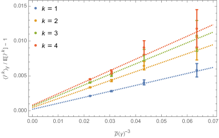
Indeed, this observation has been reported in Fig. 4 of the original article Atas:2013 that inspired this work. Equipped with the high precision of the moments of $\tilde{r}$ attained by our analytic derivation of $P_{\mathrm{c}}(a_{1},a_{2})$, we can now revisit the rather crude observation of Ref. Atas:2013 and improve it to the level of quantifying the systematic convergence of the distribution of the $\tilde{r}$-ratios of the Riemann zeroes to the GUE result (36). Mean values of the moments of $\tilde{r}_{n}$ in four windows of zeroes $[\gamma_{N},\gamma_{1.001N+1}]$ for $N=10^{8},10^{9},10^{10}$, and $103700788358$ are summarized in Table 1.

Table 1: Moments of $\tilde{r}_{n}$ for the Riemann zeroes
$N$ $\gamma_{N}$ $\langle\tilde{r}_{n}\rangle$ $\langle\tilde{r}^{2}_{n}\rangle$ $\langle\tilde{r}^{3}_{n}\rangle$ $\langle\tilde{r}^{4}_{n}\rangle$
$10^{8}$ $4.265354\cdot 10^{7}$ 0.6032357 0.4168926 0.3133507 0.2489623
$10^{9}$ $3.718702\cdot 10^{8}$ 0.6021928 0.4158748 0.3125019 0.2482868
$10^{10}$ $3.293531\cdot 10^{9}$ 0.6014386 0.4149925 0.3116161 0.2474310
103700788358 $3.058187\cdot 10^{10}$ 0.6010277 0.4145862 0.3112812 0.2471641

As the height $\gamma_{N}$ increases, relative deviations from (37), $\langle\tilde{r}^{k}_{n}\rangle/\mathbb{E}[\tilde{r}^{k}]-1$, are indeed observed to vanish systematically from above, heuristically as proportional to $\bar{\rho}(\gamma_{N})^{-3}$, indicating an approach to the complete quantum chaoticity in the ‘thermodynamic limit’ $\gamma_{N}\to\infty$ [Fig. 4].

Refer to caption
Figure 4: Relative deviations of the moments of the $\tilde{r}$-ratio $\langle\tilde{r}^{k}_{n}\rangle\ (k=1,\ldots,4)$ in four windows of the Riemann zeroes $\{\frac{1}{2}+i\gamma_{n}\}$, $n\in[N,1.001N+1]$ for $N=10^{8},10^{9},10^{10}$, and $\simeq 10^{11}$, from the GUE results $\mathbb{E}[\tilde{r}^{k}]$, plotted versus $\bar{\rho}(\gamma_{N})^{-3}$. Error bars represent statistical fluctuations due to an arbitrary choice of windows, estimated by the Jackknife method of splitting each data set in 10 bins. Dotted lines are linear fits with the least $\chi^{2}$ for each set of four points in the same color.

We remark that the systematic deviations of the statistics of the Riemann zeroes from the GUE (at infinite $N$) were previously studied in Refs. Bogomolny:2006 ; Forrester:2015 ; Bornemann:2017 . There, the ‘finite-size corrections’ in various statistical distributions for the Riemann zeroes were reported to agree well with those for the circular unitary ensemble (CUE) at finite $N_{\mathrm{eff}}\approx 1.446124\cdot\bar{\rho}(\gamma_{N})$. The relationship between these observations and our finding above will need to be clarified.

Supplementary materials

Janossy_TW_N.nb: Mathematica Notebook for generating $J_{1}(0;[a_{1},a_{2}])$ analytically by the Tracy-Widom system (33), (24) or numerically by the Nyström-type approximation (34).
Janossy_Sin.dat: numerics of $J_{1}(0;[a_{1},a_{2}])$ in the range $(a_{1},a_{2})\in[-20,0]\times[0,20]$, provided upon request by email.

Acknowledgments

I thank the LMFDB Collaboration LMFDB for making the data of the Riemann $\zeta$ function zeroes publicly downloadable, and Peter Forrester for an informative comment on the manuscript. This work is supported by JSPS Grants-in-Aids for Scientific Research (C) No.7K05416.

References

  • (1) V. Oganesyan and D.A. Huse, Localization of interacting fermions at high temperature, \PRB75,155111,2007
  • (2) Y.Y. Atas, E. Bogomolny, O. Giraud, and G. Roux, Distribution of the ratio of consecutive level spacings in random matrix ensembles, \PRE110,084101,2013
  • (3) H. Kim and D. A. Huse, Supplement of: Ballistic spreading of entanglement in a diffusive nonintegrable system, \PRL111,127205,2013
  • (4) L. D’Alessio and M. Rigol, Long-time behavior of isolated periodically driven interacting lattice systems, \PRX4,041048,2014
  • (5) D.J. Luitz, N. Laflorencie, and F. Alet, Many-body localization edge in the random-field Heisenberg chain, \PRB91,081103,2015
  • (6) Y.-Z. You, A.W.W. Ludwig, and C. Xu, Sachdev-Ye-Kitaev model and thermalization on the boundary of many-body localized fermionic symmetry protected topological states, \PRB95,115150,2017
  • (7) A.M. García-García, B. Loureiro,, A. Romero-Bermúdez, and M. Tezuka, Chaotic-integrable transition in the Sachdev-Ye-Kitaev model, \PRL120,241603,2018
  • (8) A.M. García-García, T. Nosaka, D. Rosa, and J.J.M. Verbaarschot, Quantum chaos transition in a 2-site Sachdev-Ye-Kitaev model dual to an eternal traversable wormhole, \PRD100,026002,2019
  • (9) A.M. García-García, Y. Jia, D. Rosa, and J.J.M. Verbaarschot, Sparse Sachdev-Ye-Kitaev model, quantum chaos and gravity duals, \PRD103,106002,2021
  • (10) D.-L. Deng, X. Li, and S. Das Sarma, Quantum entanglement in neural network states, \PRX7,021021,2017
  • (11) L. Zhang, J.A. Reyes, S. Kourtis, C. Chamon, E.R. Mucciolo, and A.E. Ruckenstein, Nonuniversal entanglement level statistics in projection-driven quantum circuits, \PRB101,235104,2020
  • (12) C.-M. Jian, B. Bauer, A. Keselman, and A.W.W. Ludwig, Criticality and entanglement in nonunitary quantum circuits and tensor networks of noninteracting fermions, \PRB106,134206,2022
  • (13) F. Bornemann, On the numerical evaluation of Fredholm determinants, Math. Comp., 79, 871 (2010).
  • (14) S.M. Nishigaki, Tracy-Widom method for Jánossy density and joint distribution of extremal eigenvalues of random matrices, Prog. Theor. Exp. Phys. 2021, 113A01 (2021).
  • (15) C.A. Tracy and H. Widom, Fredholm determinants, differential equations and matrix models, \CMP163,33,1994
  • (16) M.L. Mehta, Random matrices (3rd edition), Elsevier/Academic Press (Amsterdam) (2004).
  • (17) P.J. Forrester, Log-gases and random matrices, Princeton University Press (2010).
  • (18) D.J. Daley and D. Vere-Jones, An introduction to the theory of point processes, Springer-Verlag (1988).
  • (19) T. Nagao and K. Slevin, Nonuniversal correlations for random matrix ensembles, \JMP34,2075,1993
  • (20) A. Borodin and A. Soshnikov, Janossy densities I. determinantal ensembles, J. Stat. Phys., 113, 595 (2003).
  • (21) P.J. Forrester and A.M. Odlyzko, Gaussian unitary ensemble eigenvalues and Riemann $\zeta$ function zeros: A nonlinear equation for a new statistic, \PRE54,R4493,1996
  • (22) P.J. Forrester and N.S. Witte, Application of the $\tau$-function theory of Painlevé equations to random matrices: PIV, PII and the GUE, \CMP219,357,2001
  • (23) Wikipedia, Hilbert-Pólya conjecture, https://en.wikipedia.org/wiki/Hilbert-Pólya_conjecture.
  • (24) The LMFDB Collaboration, The L-functions and modular forms database, https://www.lmfdb.org/ zeros/zeta/, 2024 [online accessed July 2024].
  • (25) E. Bogomolny, O. Bohigas, P. Leboeuf, and A.G. Monastra, On the spacing distribution of the Riemann zeros: corrections to the asymptotic result, \JPA39,10743,2006
  • (26) P.J. Forrester and A. Mays, Finite size corrections in random matrix theory and Odlyzko’s data set for the Riemann zeros, Proc. R. Soc. A 471, 20150436 (2015).
  • (27) F. Bornemann, P.J. Forrester, and A. Mays, Finite size effects for spacing distributions in random matrix theory: circular ensembles and Riemann zeros, Stud. Appl. Math. 138, 401 (2017).