SoftCVI: contrastive variational inference with self-generated soft labels

Abstract

Estimating a distribution given access to its unnormalized density is pivotal in Bayesian inference, where the posterior is generally known only up to an unknown normalizing constant. Variational inference and Markov chain Monte Carlo methods are the predominant tools for this task; however, both methods are often challenging to apply reliably, particularly when the posterior has complex geometry. Here, we introduce Soft Contrastive Variational Inference (SoftCVI), which allows a family of variational objectives to be derived through a contrastive estimation framework. These objectives have zero variance gradient when the variational approximation is exact, without the need for specialized gradient estimators. The approach involves parameterizing a classifier in terms of the variational distribution, which allows the inference task to be reframed as a contrastive estimation problem, aiming to identify a single true posterior sample among a set of samples. Despite this framing, we do not require positive or negative samples, but rather learn by sampling the variational distribution and computing ground truth soft classification labels from the unnormalized posterior itself. We empirically investigate the performance on a variety of Bayesian inference tasks, using both using both simple (e.g. normal) and expressive (normalizing flow) variational distributions. We find that SoftCVI objectives often outperform other commonly used variational objectives.

1 Introduction

Consider a probabilistic model with a set of latent variables $\bm{\theta}$, for which given a set of observations ${\bm{x}_{\text{obs}}}$ we wish to infer a posterior $p(\bm{\theta}|{\bm{x}_{\text{obs}}})$. Unless the model takes a particularly convenient form, the posterior is generally only available up to an unknown normalizing constant $p(\bm{\theta}|{\bm{x}_{\text{obs}}})=p(\bm{\theta},{\bm{x}_{\text{obs}}})/p({\bm{x}_{\text{obs}}})$, where $p(\bm{\theta},{\bm{x}_{\text{obs}}})$ is available but computation of the marginal likelihood $p({\bm{x}_{\text{obs}}})$ requires an intractable integral over the latent variables $p({\bm{x}_{\text{obs}}})=\int p(\bm{\theta},{\bm{x}_{\text{obs}}})d\bm{\theta}$. In these cases, Markov chain Monte Carlo (MCMC) [28] and variational inference [37, 40] provide the two most widely used methods for performing inference, requiring only that the posterior is known up to a normalizing constant.

Variational inference involves defining a variational distribution $q_{\bm{\phi}}(\bm{\theta})$ over the set of latent variables, which is generally optimized to minimize a divergence between the variational distribution and the true posterior $p(\bm{\theta}|{\bm{x}_{\text{obs}}})$ [37, 40]. Although for certain model classes closed form solutions can be exploited [[, e.g.]]parisi1988statistical, ghahramani2000propagation, in general this is not possible, and as such many black-box methods have been developed which place minimal restrictions on the model form and variational family [59].

Variational inference is challenging to apply in many applications. Performance is hard to assess [72] and often sensitive to parameter initialization [63]. Further, the most widely used variational objective, the Evidence Lower Bound (ELBO) [40], tends to exhibit mode-seeking behavior and often produces overconfident results with lighter tails than $p(\bm{\theta}|{\bm{x}_{\text{obs}}})$. In many applications, such as scientific research, accurate uncertainty quantification (e.g. credible intervals) is crucial, yet variational posteriors are often unreliable for this task. Further, the light tails means the approximation can perform poorly in downstream tasks, such as when acting as a proposal distribution in importance sampling [8, 17, 72, 48] or for reparameterizing MCMC [28, 32]. Alternative divergences that encourage more mass-covering behavior have been proposed [42, 6, 68, 49, 22], but some research has suggested these divergences are less stable to train leading to worse performance [12, 49].

Contrastive estimation is a field in which learning is achieved by contrasting positive samples with negative samples, where the negative samples are often generated by augmenting positive samples, or by drawing samples from a carefully chosen (possibly highly structured) noise distribution [25, 50]. Among other use cases, contrastive learning has been widely employed for representation learning [50, 29, 9] and for performing inference when the likelihood function is only available through an intractable integral, such as for fitting energy-based models [61, 16, 27, 60] or for performing simulation-based inference [30, 66, 13, 46, 27]. Contrastive estimation often utilizes classification objectives, and a common theme is to exploit the invariance of the objective to unknown normalizing constants in order to facilitate learning.

Contribution
We show that contrastive estimation can be used to derive a family of variational objectives, terming the approach Soft Contrastive Variational Inference (SoftCVI). The task of fitting the posterior approximation is reframed as a classification task, aiming to identify a single true posterior sample among a set of samples. Instead of using explicitly positive and negative samples, we show that for arbitrary samples from a proposal distribution, we can generate ground truth soft classification labels using the unnormalized posterior density itself. The samples alongside the labels are used for fitting a classifier parameterized in terms of the variational distribution, such that the optimal classifier recovers the true posterior. A series of experiments are performed, showing that the method produces posteriors with good coverage properties and performs favorably compared to alternative variational inference methods. We provide a pair of Python packages, softcvi and softcvi_validation, which provide the implementation, and the code for reproducing the results of this manuscript, respectively.

2 SoftCVI

In order to fit a variational distribution with SoftCVI, we must define a proposal distribution $\pi(\bm{\theta})$, a negative distribution $p^{-}(\bm{\theta})$, and a variational distribution $q_{\bm{\phi}}(\bm{\theta})$, which generally are defined to be supported on the same set as the true posterior $p(\bm{\theta}|{\bm{x}_{\text{obs}}})$. At each optimization step, three steps are performed which allow fitting the variational distribution:

1. Sample latent variables $\{\bm{\theta}_{k}\}_{k=1}^{K}\sim\pi(\bm{\theta})$ from the proposal distribution $\pi(\bm{\theta})$.

2. Generate corresponding ground truth soft labels $\bm{y}\in(0,1)^{K}$ for the task of classifying between positive and negative samples, presumed to be from $p(\bm{\theta}|{\bm{x}_{\text{obs}}})$ and $p^{-}(\bm{\theta})$, respectively.

3. Use $\{\bm{\theta}_{k}\}_{k=1}^{K}$ along with the soft labels $\bm{y}$ to optimize a classifier parameterized in terms of the variational distribution $q_{\bm{\phi}}(\bm{\theta})$, such that the optimal classifier recovers the true posterior.

The choice of proposal distribution in step 1 will influence the region in which learning is focused. Throughout the experiments here, we take the intuitive choice of using the variational distribution itself as the proposal distribution $\pi(\bm{\theta})=q_{\bm{\phi}}(\bm{\theta})$, which over the course of training directs learning towards regions with reasonable posterior mass.

2.1 Generating ground truth soft labels

Consider for simplicity the case that we have access to positive (true posterior) and negative samples. Specifically, consider the scenario in which we have $K$ samples $\{\bm{\theta}_{k}\}_{k=1}^{K}$, consisting of exactly one positive sample from the true posterior $p(\bm{\theta}|{\bm{x}_{\text{obs}}})$, and $K-1$ negative samples from a negative distribution $p^{-}(\bm{\theta})$. The optimal classifier can be parameterized in terms of the ratio between the positive and negative densities $p(\bm{\theta}|{\bm{x}_{\text{obs}}})/p^{-}(\bm{\theta})$ [[, e.g]]gutmann2012noise, oord2018representation, thomas2022likelihood. Letting $k^{*}$ denote the index of the true sample, and assuming each element $\bm{\theta}_{k}$ is equally likely to be the true sample a priori, the optimal classifier is

$$y_{k} =P(k^{*}=k|\{\bm{\theta}_{k}\}_{k=1}^{K},{\bm{x}_{\text{obs}}})=\frac{p(\bm{\theta}_{k}|{\bm{x}_{\text{obs}}})/p^{-}(\bm{\theta}_{k})}{\sum_{k^{\prime}=1}^{K}p(\bm{\theta}_{k^{\prime}}|{\bm{x}_{\text{obs}}})/p^{-}(\bm{\theta}_{k^{\prime}})},$$ (1)

where $y_{k}=P(k^{*}=k|\{\bm{\theta}_{k}\}_{k=1}^{K},{\bm{x}_{\text{obs}}})$ is the probability on the interval $(0,1)$ that $\bm{\theta}_{k}$ is the positive sample $\bm{\theta}_{k^{*}}$ among all the considered samples, and $\sum_{k=1}^{K}y_{k}=1$. The above computation is invariant to multiplicative constants to the ratio $p(\bm{\theta}|{\bm{x}_{\text{obs}}})/p^{-}(\bm{\theta})$, meaning that although $p(\bm{\theta}|{\bm{x}_{\text{obs}}})$ is generally unknown, the unnormalized version $p(\bm{\theta},{\bm{x}_{\text{obs}}})\propto p(\bm{\theta}|{\bm{x}_{\text{obs}}})$, is sufficient for computing the optimal labels

$$y_{k} =\frac{p(\bm{\theta}_{k},{\bm{x}_{\text{obs}}})/p^{-}(\bm{\theta}_{k})}{\sum_{k^{\prime}=1}^{K}p(\bm{\theta}_{k^{\prime}},{\bm{x}_{\text{obs}}})/p^{-}(\bm{\theta}_{k^{\prime}})},$$

$$\bm{y} =\operatorname{softmax}(\bm{z}),\quad\text{ where }z_{k}=\log\frac{p(\bm{\theta}_{k},{\bm{x}_{\text{obs}}})}{p^{-}(\bm{\theta}_{k})}.$$ (2)

Intuitively, the ratio $p(\bm{\theta}_{k},{\bm{x}_{\text{obs}}})/p^{-}(\bm{\theta}_{k})$ encodes the relative likelihood of a sample $\bm{\theta}_{k}$ being the true sample, and to compute the labels the ratios are normalized over the set of considered samples.

Contrastive estimation methods generally use explicitly positive and negative examples, with hard labels $\bm{y}\in\{0,1\}^{K}$. However, in this context, we do not have access to positive samples from $p(\bm{\theta}|{\bm{x}_{\text{obs}}})$, and we may not have access to samples from $p^{-}(\bm{\theta})$. Nonetheless, despite the framing of the classification task, we can instead generate samples from a proposal distribution, $\{\bm{\theta}_{k}\}_{k=1}^{K}\sim\pi(\bm{\theta})$, and by assigning labels to these samples it is still possible to train a classifier which at optimality recovers the true posterior, which we will discuss in the subsequent section.

2.2 Parameterization and optimization of the classifier

Analogously to the computation of the labels in eq. 1, we can parameterize the classifier in terms of the ratio between the variational and negative distribution

$$\hat{y}_{k} =\frac{q_{\bm{\phi}}(\bm{\theta}_{k})/p^{-}(\bm{\theta}_{k})}{\sum_{k^{\prime}=1}^{K}q_{\bm{\phi}}(\bm{\theta}_{k^{\prime}})/p^{-}(\bm{\theta}_{k^{\prime}})}$$

$$\hat{\bm{y}} =\operatorname{Softmax}(\hat{\bm{z}}),\quad\text{where }\hat{z}_{k}=\log\frac{q_{\bm{\phi}}(\bm{\theta}_{k})}{p^{-}(\bm{\theta}_{k})},$$ (3)

Given a set of samples $\{\bm{\theta}_{k}\}_{k=1}^{K}$ and corresponding labels $\bm{y}$, an optimization step can be taken to minimize the softmax cross-entropy loss function (i.e. the negative multinomial log-likelihood)

$$\mathcal{L}(\bm{\phi};\{\bm{\theta}_{k}\}_{k=1}^{K},\bm{y})=-\sum_{k=1}^{K}y_{k}\log\left(\frac{q_{\bm{\phi}}(\bm{\theta}_{k})/p^{-}(\bm{\theta}_{k})}{\sum_{k^{\prime}=1}^{K}q_{\bm{\phi}}(\bm{\theta}_{k^{\prime}})/p^{-}(\bm{\theta}_{k^{\prime}})}\right).$$ (4)

Assuming $q_{\bm{\phi}}(\bm{\theta})$ is sufficiently flexible, the optimal classifier outputs labels matching the ground truth labels, $\bm{y}=\hat{\bm{y}}$, across the support of the proposal distribution $\pi(\bm{\theta})$. Equivalently, this suggests the classifier must learn the density ratio between the positive and negative distributions up to a constant

$$p(\bm{\theta}|{\bm{x}_{\text{obs}}})/p^{-}(\bm{\theta}) =c\cdot q_{\bm{\phi}}(\bm{\theta})/p^{-}(\bm{\theta}),$$

$$p(\bm{\theta}|{\bm{x}_{\text{obs}}}) =c\cdot q_{\bm{\phi}}(\bm{\theta}).$$ (5)

Assuming that the support of $$\pi(\bm{\theta}) p(\bm{\theta}|{\bm{x}_{\text{obs}}}) q_{\bm{\phi}}(\bm{\theta})$$ is a superset of the supports of both and , the optimal classifier recovers the true posterior

$$\int_{\text{supp}(\pi)}p(\bm{\theta}|{\bm{x}_{\text{obs}}})d\bm{\theta} =c\cdot\int_{\text{supp}(\pi)}q_{\bm{\phi}}(\bm{\theta})d\bm{\theta},$$

$$c=1,$$

$$p(\bm{\theta}|{\bm{x}_{\text{obs}}}) =q_{\bm{\phi}}(\bm{\theta}).$$ (6)

Further, we demonstrate in appendix A that when the optimal classifier is achieved, the gradient is zero (and consequently has zero variance) for finite $K$. This is a generally desirable property that is not present in many variational objectives, although specialized gradient estimators have been developed which in some cases can address this issue [62, 67].

2.3 Choice of the negative distribution

The choice of negative distribution $p^{-}(\bm{\theta})$ alters the implied classification problem and the resulting objective. Separating out the log term, we can rewrite the softmax cross entropy objective from eq. 4 as

$$\mathcal{L}(\bm{\phi};\{\bm{\theta}_{k}\}_{k=1}^{K},\bm{y}) =-\sum_{k=1}^{K}y_{k}\log q_{\bm{\phi}}(\bm{\theta}_{k})+\log\sum_{k=1}^{K}\frac{q_{\bm{\phi}}(\bm{\theta}_{k})}{p^{-}(\bm{\theta}_{k})}+\text{const},$$ (7)

where the first term encourages placing posterior mass on the samples likely to be from the true posterior, and the second term penalizes the sum of the ratios. The choice of negative distribution has a large impact on the behavior of the objective, particularly for samples with (comparatively) negligible posterior mass. Such samples tend to have labels close to zero, and thus primarily influence the loss through the second term in eq. 7. This suggests that a choice of $p^{-}(\bm{\theta})$ similar to the posterior would heavily punish placing mass in $q_{\bm{\phi}}(\bm{\theta})$ where there is negligible posterior mass, causing more mode seeking behavior. In contrast, choosing an improper flat distribution as the negative distribution would only weakly punish “leakage” of mass into regions of negligible posterior density, with the second term reducing to $\log\sum_{k=1}^{K}q_{\bm{\phi}}(\bm{\theta}_{k})+\text{const}$. Here, we focus on setting $p^{-}(\bm{\theta})=q_{\bm{\phi}}(\bm{\theta})^{\alpha}$, where $\alpha\in[0,1]$ is a tempering hyperparameter which interpolates between directly using the variational distribution as the negative distribution (when $\alpha=1$) and using a flat (improper) negative distribution (when $\alpha=0$).

The overall approach of SoftCVI is shown in algorithm 1. Note that although $p^{-}(\bm{\theta})$ is parameterized using $q_{\bm{\phi}}(\bm{\theta})$, we hold the parameters of $p^{-}(\bm{\theta})$ constant when computing the objective gradient, using the stop gradient operator.

Inputs: $p(\bm{\theta},{\bm{x}_{\text{obs}}})$, $p^{-}(\bm{\theta})$, $q_{\bm{\phi}_{1}}(\bm{\theta})$, number of samples $K\geq 2$, optimization steps $N$, learning rate $\eta$

for $i$ in $1:N$ do

      1 Sample $\{\bm{\theta}_{k}\}_{k=1}^{K}\sim\pi(\bm{\theta})$

      2 Compute soft labels $\bm{y}=\operatorname{Softmax}(\bm{z}),\text{ where }z_{k}=\log\frac{p(\bm{\theta}_{k},{\bm{x}_{\text{obs}}})}{p^{-}(\bm{\theta}_{k})}$

      3 Update $\bm{\phi}_{i+1}=\bm{\phi}_{i}-\eta\nabla_{\bm{\phi}}\mathcal{L}(\bm{\phi}_{i};\{\bm{\theta}_{k}\}_{k=1}^{K},\bm{y})$ using the cross-entropy loss, eq. 4

end for

Algorithm 1 SoftCVI

3 Experiments

We evaluate the performance on a variety of Bayesian inference tasks for which reference (ground truth) posterior samples, $\{\bm{\theta}^{*}_{i}\}_{i=1}^{N_{\text{ref}}}$, are available. We focus results on two choices of negative distribution, parameterized as $q_{\bm{\phi}}(\bm{\theta})^{\alpha}$ with $\alpha=0.75$ and $\alpha=1$. We compare performance to variational inference either with the ELBO, or the more mass-covering Self-Normalized Importance Sampling Forward Kullback-Leibler (SNIS-fKL) divergence [36, 22], and we leave descriptions of these until section 5.1. For each task, we perform 20 independent runs with different random seeds. Where possible (i.e. an analytical posterior is available), we use a different observation for every run. For tasks where the reference posterior is created through sampling methods we rely on reference posteriors provided by PosteriorDB [45] or SBI-Benchmark [43] and for each run we sample from the available observations if multiple options are present. We run all considered methods for 100,000 optimization steps, using the adam optimizer [39], and a learning rate of $1e^{-3}$. For all methods, we use $K=8$ samples from $q_{\bm{\phi}}(\bm{\theta})$ during computation of the objective.

Software: Our implementation and experiments made wide use of the python packages jax [5], equinox [38], numpyro [57], flowjax [70] and optax [11].

3.1 Metrics

Coverage probabilities. Posterior coverage probabilities have been widely used to assess the reliability of posteriors [[, e.g.]]cook2006validation, talts2018validating, prangle2014diagnostic, hermans2021trust, ward2022robust, cannon2022investigating. Given a nominal frequency $\gamma\in[0,1]$, the metric assesses the frequency at which true posterior samples fall within the $100\gamma\%$ highest posterior density region (credible region) of the approximate posterior. If the actual frequency is greater than $\gamma$, the posterior is conservative for that coverage probability. If the frequency is less, then the posterior is overconfident. A posterior is said to be well calibrated if the actual frequency matches $\gamma$ for any choice of $\gamma$. A well calibrated, or somewhat conservative posterior is needed for drawing reliable scientific conclusions, and as such is an important property to investigate. For a nominal $\gamma$, we estimate the actual coverage frequency for a posterior estimate as

$$\frac{1}{N_{\text{ref}}}\sum_{i=1}^{N_{\text{ref}}}\mathds{1}\left\{{\bm{\theta}_{i}^{*}\in\operatorname{HDR}_{q_{\bm{\phi}}(\bm{\theta}|{\bm{x}_{\text{obs}}})}(\gamma)}\right\}$$ (8)

where $\mathds{1}$ is the indicator function, and $\operatorname{HDR}$ represents the highest posterior density region, inferred using the density quantile approach of [35].

Log probability of $\bm{\theta}^{*}$. Looking at the probability of either reference posterior samples or the ground truth parameters in a posterior approximation is a common metric for assessing performance [[, e.g.]]lueckmann2021benchmarking, papamakarios2016fast, greenberg2019automatic. The quantity is likely a good indicator of how well the approximation would perform in downstream tasks, for example, as it is known to control error in importance sampling [8]. We compute this independently for each posterior approximation as follows

$$\frac{1}{N_{\text{ref}}}\sum_{i=1}^{N_{\text{ref}}}\log q_{\bm{\phi}}(\bm{\theta}^{*}_{i}).$$ (9)

This metric also approximates the negative forward KL-divergence between the true and approximate posterior up to a constant

$$-D_{\text{KL}}[p(\bm{\theta}|{\bm{x}_{\text{obs}}})||q_{\bm{\phi}}(\bm{\theta})] =-\mathbb{E}_{p(\bm{\theta}|{\bm{x}_{\text{obs}}})}[\log p(\bm{\theta}|{\bm{x}_{\text{obs}}})-\log q_{\bm{\phi}}(\bm{\theta})],$$

$$\approx\frac{1}{N_{\text{ref}}}\sum_{i=1}^{N_{\text{ref}}}\log q_{\bm{\phi}}(\bm{\theta}_{i}^{*})+\text{const}.$$ (10)

Posterior mean accuracy. A posterior that is overconfident, but unbiased would perform poorly based on the aforementioned metrics, but could form good point estimates for the latent variables. Although the exact metric may vary, the accuracy of point estimates has been widely used in Bayesian inference [[, e.g.]]gerwinn2010bayesian, baudart2021automatic, ma2011bayesian. Here, we choose to measure the accuracy using the negative $L^{2}$-norm (Euclidean distance) of the standardized difference in posterior means

$$-\left\lVert\frac{\text{mean}(\bm{\theta}^{*})-\text{mean}(\bm{\theta})}{\text{std}(\bm{\theta}^{*})}\right\rVert_{2},$$ (11)

where $\text{mean}(\bm{\theta}^{*})$ and $\text{mean}(\bm{\theta})$ are the mean vectors of the reference and posterior approximation samples respectively, and $\text{std}(\bm{\theta}^{*})$ is the vector of standard deviations of the reference samples.

3.2 Tasks

Where possible, we make use of reparameterizations (such as non-centering) to reduce the dependencies between the latent variables, and ensure variables are reasonably scaled, which is generally considered to improve performance [54, 23, 3].

Eight schools: The eight schools model is a classic hierarchical Bayesian inference problem, where the aim is to infer the treatment effects of a coaching program applied to eight schools, which are assumed to be exchangeable [64, 18]. The parameter set is $\bm{\theta}=\{\mu,\tau,\bm{m}\}$, where $\mu$ is the average treatment effect across the schools, $\tau$ is the standard deviation of the treatment effects across the schools and $\bm{m}$ is the eight-dimensional vector of treatment effects for each school. For the posterior approximation $q_{\bm{\phi}}(\bm{\theta})$, we use a normal distribution for $\mu$, a folded Student’s t distribution for $\tau$ (where folding is equivalent to taking an absolute value transform), and a Student’s t distribution for $\bm{m}$. We use the reference posterior samples available from PosteriorDB [45].

Linear regression: We consider a linear regression model, with parameters $\bm{\theta}=\{\bm{\beta},\mu\}$, where $\bm{\beta}\in\mathbb{R}^{50}$ is the regression coefficients, and $\mu\in\mathbb{R}$ is the bias parameter. The covariates $\bm{X}\in\mathbb{R}^{(200\times 50)}$ are generated from a standard normal distribution, with targets sampled according to $\bm{y}\sim N(\bm{X}\bm{\beta}+\mu,1)$. The posterior approximation $q_{\bm{\phi}}(\bm{\theta})$ is implemented as a fully factorized normal distribution. This task yields an analytical form for the posterior.

SLCP: The Simple Likelihood Complex Posterior (SLCP) task introduced in [53], parameterizes a multivariate normal distribution using a 5-dimensional vector $\bm{\theta}$. Due to squaring in the parameterization, the posterior contains four symmetric modes. Further, a uniform prior $\{\bm{\theta}_{i}\}_{i=1}^{5}\sim\text{Uniform}(-3,3)$ is used, which introduces sharp cut-offs in the posterior density, making the task a challenging inference problem. For the posterior approximation $q_{\bm{\phi}}(\bm{\theta})$, we use an 8 layer masked autoregressive flow [52, 41, 19], with a rational quadratic spline transformer [14]. We use the observations and reference posteriors available from the SBI-Benchmark package [43].

GARCH(1,1): A Generalized Autoregressive Conditional heteroscedasticity (GARCH) model [4]. GARCH models are used for modeling the changing volatility of time series data by accounting for time-varying and autocorrelated variance in the error terms. The observation consists of a 200-dimensional time series $\bm{x}$, where each element $x_{t}$ is drawn from a normal distribution with mean $\mu$ and time-varying variance $\sigma_{t}^{2}$. The variance $\sigma_{t}^{2}$ is defined recursively by the update

$$\sigma^{2}_{t}=\alpha_{0}+\alpha_{1}(x_{t-1}-\mu)^{2}+\beta_{1}\sigma^{2}_{t-1}$$ (12)

To parameterize $q_{\bm{\phi}}(\bm{\theta})$, we use a normal distribution for $\mu$ and a log normal distribution for $\alpha_{0}$. For $\alpha_{1}$ and $\beta_{1}$ we use uniform distributions constrained to the prior support, transformed with a rational quadratic spline. To allow modeling of posterior dependencies, the distribution over $\beta_{1}$ is parameterized as a function of $\alpha_{1}$ and $\alpha_{2}$ using a neural network. We use the reference posterior samples available from PosteriorDB [45].

4 Results

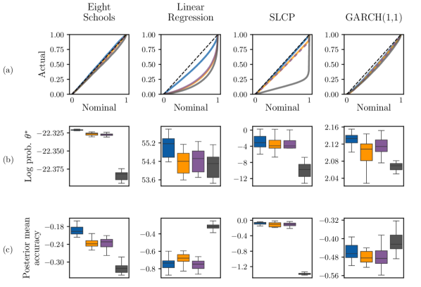
Figure 1: The posterior performance metrics (see section 3.1). a) The nominal coverage frequency against the actual coverage frequency, averaged across the runs. Methods producing well-calibrated posteriors would follow $y=x$ (shown as a black dashed line), whereas methods tending to be conservative fall above the line, and overconfident methods fall below the line. Where lines overlap significantly we use dashed lines to aid visualization. b) The average probability of the reference posterior samples in the approximate posterior. c) The accuracy of the approximate posteriors mean, calculated as the negative l2-norm of the standardized difference between the mean of the approximate and reference posterior samples.

Across all tasks and metrics considered, the SoftCVI derived objectives performed competitively with the ELBO and SNIS-fKL objectives (fig. 1). Overall, SoftCVI using a negative distribution $q_{\bm{\phi}}(\bm{\theta})^{\alpha}$ with $\alpha=1$ led to performance very similar to SNIS-fKL across all the metrics. However, setting $\alpha=0.75$ to slightly temper the negative distribution leads to SoftCVI outperforming all the other approaches, particularly tending to yield better calibrated posteriors and placing more mass on average on the reference posterior samples.

The SLCP task yields complex posterior geometry, with four symmetric modes. For this task, the ELBO-trained posteriors had coverage frequencies approaching approximately $\frac{1}{4}$ for nominal coverage frequencies near $1$, suggesting that frequently only one of the four modes is recovered (fig. 1). From inspecting individual posteriors, we can confirm this to be the case, whilst in contrast both SoftCVI and SNIS-fKL tend to recover all four modes (fig. 2).

To illustrate the impact of the choice of negative distribution, fig. 2 also shows a posterior trained with a flat negative distribution by setting $\alpha=0$. It is clear that a flat negative distribution does not sufficiently penalize placing mass in $q_{\bm{\phi}}(\bm{\theta})$ in regions of negligible posterior density (see section 2.3), leading to “leakage” of mass.

Overall, these results suggest SoftCVI to provide a framework for deriving performant and robust objectives for variational inference, including for models which exhibit posteriors with complex geometry.

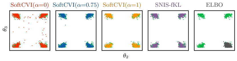
Figure 2: A 2-dimensional posterior marginal for a single run of the SLCP task, with the reference posterior samples shown in green. The ELBO objective leads to mode-seeking behaviour, whereas the other objectives tend to discover all the modes. We also show the posterior for SoftCVI with $\alpha=0$.

5 Related work

5.1 Variational inference

ELBO

In variational inference, the most commonly used training objective is to minimize the negative ELBO, or equivalently, minimizing the reverse Kullback-Leibler (KL) divergence between the posterior approximation and the true posterior

$$D_{KL}[q_{\bm{\phi}}(\bm{\theta})||p(\bm{\theta}|{\bm{x}_{\text{obs}}})] =\mathbb{E}_{q_{\bm{\phi}}(\bm{\theta})}\left[\log q_{\bm{\phi}}(\bm{\theta})-\log p(\bm{\theta}|{\bm{x}_{\text{obs}}})\right],$$ (13)

$$=\mathbb{E}_{q_{\bm{\phi}}(\bm{\theta})}[\log q_{\bm{\phi}}(\bm{\theta})-\log p(\bm{\theta},{\bm{x}_{\text{obs}}})]+\text{const}.$$ (14)

As there is no general closed-form solution for the divergence, a Monte Carlo approximation is often used [40]

$$\mathcal{L}_{\text{ELBO}}(\bm{\phi}) =\frac{1}{K}\sum_{k=1}^{K}\left[\log q_{\bm{\phi}}(\bm{\theta}_{k})-\log p(\bm{\theta}_{k},{\bm{x}_{\text{obs}}})\right],\text{ where }\{\bm{\theta}_{k}\}_{k=1}^{K}\sim q_{\bm{\phi}}(\bm{\theta}),$$ (15)

Although straightforward to apply, the reverse KL divergence heavily punishes placing mass in regions with little mass in the true posterior, leading to mode-seeking behavior and lighter tails than $p(\bm{\theta}|{\bm{x}_{\text{obs}}})$.

SNIS-fKL

An alternative approach, introduced by [36], instead uses self-normalized importance sampling to estimate the forward KL divergence, which is more mass-covering. Specifically, an importance weighted estimate of the forward KL divergence is given by

$$D_{KL}[p(\bm{\theta}|{\bm{x}_{\text{obs}}})||q_{\bm{\phi}}(\bm{\theta})] =\mathbb{E}_{p(\bm{\theta}|{\bm{x}_{\text{obs}}})}\left[\log\frac{p(\bm{\theta},{\bm{x}_{\text{obs}}})}{q_{\bm{\phi}}(\bm{\theta})}\right]+\text{const},$$ (16)

$$=\mathbb{E}_{\pi(\bm{\theta})}\left[w(\bm{\theta})\log\frac{p(\bm{\theta},{\bm{x}_{\text{obs}}})}{q_{\bm{\phi}}(\bm{\theta})}\right]+\text{const},$$ (17)

where $w(\bm{\theta})=p(\bm{\theta}|{\bm{x}_{\text{obs}}})/\pi(\bm{\theta})$ is the importance weights. By sampling $\{\bm{\theta}_{k}\}_{k=1}^{K}\sim\pi(\bm{\theta})$, we can compute a set of self-normalized weights

$$\tilde{w}(\bm{\theta}_{k})=\frac{p(\bm{\theta}_{k},{\bm{x}_{\text{obs}}})/\pi(\bm{\theta}_{k})}{\sum_{k^{\prime}=1}^{K}p(\bm{\theta}_{k^{\prime}},{\bm{x}_{\text{obs}}})/\pi(\bm{\theta}_{k^{\prime}})},$$ (18)

and use a self-normalized importance sampling scheme to estimate the forward KL, which introduces bias vanishing with order $\mathcal{O}(1/K)$ [1]

$$\mathcal{L}_{\text{SNIS-fKL}}(\bm{\phi};\{\bm{\theta}_{k}\}_{k=1}^{K})=\sum_{k=1}^{K}\tilde{w}(\bm{\theta}_{k})\log\frac{p(\bm{\theta}_{k},{\bm{x}_{\text{obs}}})}{q_{\bm{\phi}}(\bm{\theta}_{k})}.$$ (19)

We use $\pi(\bm{\theta})=q_{\bm{\phi}}(\bm{\theta})$, and follow the gradient estimator from [22], which holds the proposal parameters constant under differentiation. There are some similarities between the SNIS-fKL objective, and the SoftCVI objectives, which we discuss in appendix C.

5.2 Contrastive learning

Contrastive learning most commonly allows learning of distributions through the comparison of true samples, to a set of negative (noise or augmented) samples [25]. Probably the most widely used objective function in contrastive learning is the InfoNCE loss, proposed by [50]. Given a set of samples $\{\bm{\theta}_{k}\}_{k=1}^{K}$, containing a single true sample with index $k^{*}$, the loss can be computed as

$$\text{InfoNCE}(\bm{\phi};\{\bm{\theta}_{k}\}_{k=1}^{K})=-\log\frac{f_{\bm{\phi}}(\bm{\theta}_{k^{*}})}{\sum_{k=1}^{K}f_{\bm{\phi}}(\bm{\theta}_{k})}.$$ (20)

where $f_{\bm{\phi}}(\bm{\theta})$ approximates the ratio between true and noise distribution samples (up to a constant). In practice this is usually shown with an additional sum (or expectation) over different sets of $\{\bm{\theta}_{k}\}_{k=1}^{K}$. Note that the above objective can also be derived from the softmax cross entropy objective used by SoftCVI, eq. 4, by inputting a one-hot encoded vector of labels $\bm{y}$ with $y_{k^{*}}=1$, and the other values $0$. Recently, there has been much investigation of the use of soft (or ranked) labels in contrastive learning [15, 33], including using cross-entropy-like loss functions [34, 56]. However, these methods generally assume the dataset contains labels, or that we can approximate labels using similarity metrics between true and augmented samples. In contrast, here we compute ground truth labels utilizing access to a likelihood function.

Contrastive learning has also been widely applied in simulation-based inference, for learning posteriors [66, 14, 30, 24, 46, 27]. In this context, the likelihood is assumed to be intractable, and the classifier is parameterized to learn the ratio between joint samples $p(\bm{\theta},\bm{x})$ and marginal samples $p(\bm{x})p(\bm{\theta})$ up to a constant. Some variants of the sequential neural posterior estimation algorithm, similar to the current work, parameterize the classifier in terms of a normalized approximation of the posterior, and utilize the current posterior estimate as a proposal distribution [24, 14]. Here, we demonstrate that the choice of the negative distribution changes the behavior of the posterior approximations, particularly with the degree of posterior leakage (fig. 2), which could suggest avenues for improvement for sequential neural posterior estimation methods, which often have problematic leakage [13].

Contrastive learning is a large field of research that undoubtedly provides opportunities for further extensions of SoftCVI; for example, it may be interesting to investigate how commonly used techniques in classification and contrastive learning, such as label smoothing [47] or temperature parameters [69], could be used to improve training stability and control the calibration of the posterior.

6 Conclusion

In this work, we introduce SoftCVI, a framework for deriving variational objectives using contrastive estimation, and apply it to a range of Bayesian inference tasks. Use of the method is as simple as exchanging the objective function in a probabilistic programming language that supports black-box variational inference. Initial experiments indicate that SoftCVI frequently outperforms variational inference with either the ELBO or SNIS-fKL objectives, across various tasks and with different variational families. To the best of our knowledge this constitutes a novel method, which bridges between variational inference and contrastive estimation, and opens up new avenues for both theoretical and practical research.

Appendix A Zero variance gradient at optimum with finite K

When the optimal classifier is reached, we can show that the gradient is zero (and hence has zero variance), even for finite $K$. To avoid clashes with the parameters $\bm{\phi}$, we will use superscripts for indices. We have the objective

$$\mathcal{L}(\bm{\phi};\{\bm{\theta}^{k}\}_{k=1}^{K},\bm{y}) =-\sum_{k=1}^{K}y^{k}\log\left(\frac{q_{\bm{\phi}}(\bm{\theta}^{k})/p^{-}(\bm{\theta}^{k})}{\sum_{k^{\prime}=1}^{K}q_{\bm{\phi}}(\bm{\theta}^{k^{\prime}})/p^{-}(\bm{\theta}^{k^{\prime}})}\right),$$ (21)

Letting $$\hat{y}_{\bm{\phi}}^{k}$$ replace the term inside the log

$$=-\sum_{k=1}^{K}y^{k}\log\hat{y}_{\bm{\phi}}^{k},$$ (22)

$$\nabla\mathcal{L}(\bm{\phi};\{\bm{\theta}^{k}\}_{k=1}^{K},\bm{y}) =-\sum_{k=1}^{K}y^{k}\nabla\log\hat{y}_{\bm{\phi}}^{k},$$ (23)

$$=-\sum_{k=1}^{K}y^{k}\frac{\nabla\hat{y}_{\bm{\phi}}^{k}}{\hat{y}_{\bm{\phi}}^{k}},$$ (24)

which due to optimality of the classifier we have $$y^{k}=\hat{y}_{\bm{\phi}}^{k}$$

$$=-\sum_{k=1}^{K}\nabla\hat{y}_{\bm{\phi}}^{k},$$ (25)

due to the properties of the softmax, the labels must sum to 1

$$=-\nabla\sum_{k=1}^{K}\hat{y}_{\bm{\phi}}^{k}=\bm{0}.$$ (26)

Appendix B Additional results

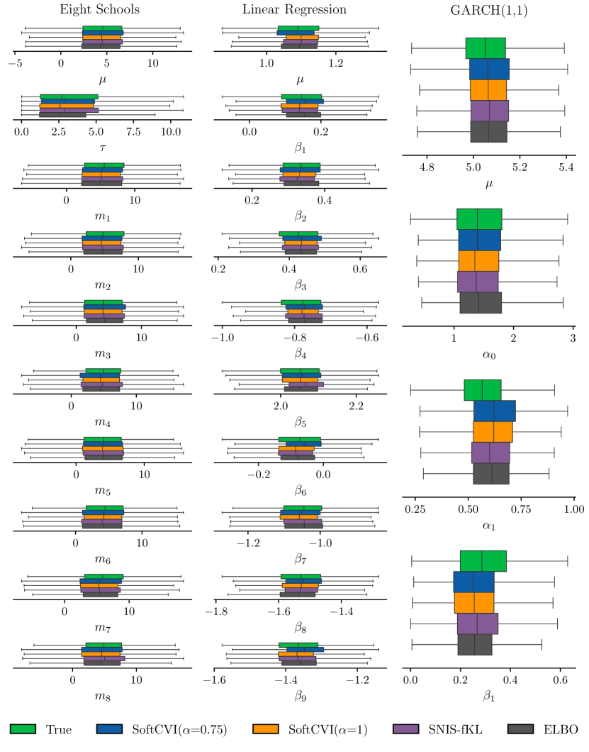
Figure 3: The distribution of the posterior marginals for a single run of the eight schools, linear regression and GARCH (1,1) tasks. For the linear regression task, we restrict the plot to the first 10 parameters of the model.

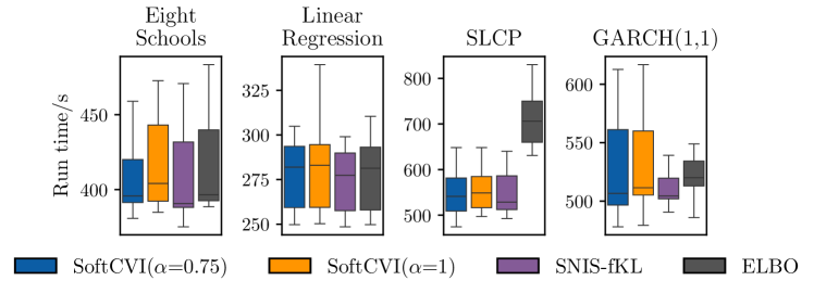
Figure 4: The run times including compilation time for each task using $k=8$ (CPU, 8GB RAM).

Appendix C Comparison to SNIS-fKL

Taking the form of the SoftCVI objective from eq. 7, we have

$$\mathcal{L}_{\text{SoftCVI}}(\bm{\phi};\{\bm{\theta}_{k}\}_{k=1}^{K},\bm{y}) =-\sum_{k=1}^{K}y_{k}\log q_{\bm{\phi}}(\bm{\theta}_{k})+\log\sum_{k=1}^{K}\frac{q_{\bm{\phi}}(\bm{\theta}_{k})}{p^{-}(\bm{\theta}_{k})}+\text{const}.$$ (27)

Choosing to ignore the constant, and assuming we choose both $p^{-}(\bm{\theta})$ and $\pi(\bm{\theta})$ to be equal to $q_{\bm{\phi}}(\bm{\theta})$, we have

$$=-\sum_{k=1}^{K}y_{k}\log q_{\bm{\phi}}(\bm{\theta}_{k})+\log\sum_{k=1}^{K}\frac{q_{\bm{\phi}}(\bm{\theta}_{k})}{\pi(\bm{\theta}_{k})},$$ (28)

where

$$y_{k}=\frac{p(\bm{\theta}_{k},{\bm{x}_{\text{obs}}})/\pi(\bm{\theta}_{k})}{\sum_{k^{\prime}=1}^{K}p(\bm{\theta}_{k^{\prime}},{\bm{x}_{\text{obs}}})/\pi(\bm{\theta}_{k^{\prime}})}.$$ (29)

As for the SNIS-fKL objective in eq. 19, the numerator term does not depend on $\bm{\phi}$, we have

$$\mathcal{L}_{\text{SNIS-fKL}}(\bm{\phi})=-\sum_{k=1}^{K}\tilde{w}(\bm{\theta}_{k})\log q_{\bm{\phi}}(\bm{\theta}_{k})+\text{const}$$ (30)

Noticing that the self-normalized weights, eq. 18, and the ground truth labels $y_{k}$ are computed identically, the losses (ignoring constants) only differ by the normalization term

$$\mathcal{L}_{\text{SoftCVI}}(\bm{\phi})=\mathcal{L}_{\text{SNIS-fKL}}(\bm{\phi})+\log\sum_{k=1}^{K}\frac{q_{\bm{\phi}}(\bm{\theta}_{k})}{\pi(\bm{\theta}_{k})}.$$ (31)

At optimality of the classifier, the SoftCVI objective yields zero variance gradient estimates (see appendix A). Along with eq. 31, this suggests the variance of SNIS-fKL gradient is equal to the variance of the gradient of the normalization term, which generally is not zero. This suggests an advantage to using the SoftCVI objective; the gradient variance will decrease as the variational distribution approaches the posterior, similar to the sticking the landing estimator [62]. For other choices of $p^{-}(\bm{\theta})$ in SoftCVI, the differences between the methods become more significant and direct comparison becomes challenging.

References

- [1] Sergios Agapiou, Omiros Papaspiliopoulos, Daniel Sanz-Alonso and Andrew M Stuart “Importance sampling: Intrinsic dimension and computational cost” In Statistical Science JSTOR, 2017, pp. 405–431
- [2] Guillaume Baudart and Louis Mandel “Automatic guide generation for Stan via NumPyro” In arXiv preprint arXiv:2110.11790, 2021
- [3] Michael Betancourt and Mark Girolami “Hamiltonian Monte Carlo for hierarchical models” In Current trends in Bayesian methodology with applications 79.30 CRC Press Boca Raton, FL, 2015, pp. 2–4
- [4] Tim Bollerslev “Generalized autoregressive conditional heteroskedasticity” In Journal of econometrics 31.3 Elsevier, 1986, pp. 307–327
- [5] James Bradbury et al. “JAX: composable transformations of Python+NumPy programs”, 2018 URL: http://github.com/google/jax
- [6] Yuri Burda, Roger Grosse and Ruslan Salakhutdinov “Importance weighted autoencoders” In arXiv preprint arXiv:1509.00519, 2015
- [7] Patrick Cannon, Daniel Ward and Sebastian M Schmon “Investigating the impact of model misspecification in neural simulation-based inference” In arXiv preprint arXiv:2209.01845, 2022
- [8] Sourav Chatterjee and Persi Diaconis “The sample size required in importance sampling” In The Annals of Applied Probability 28.2 JSTOR, 2018, pp. 1099–1135
- [9] Ting Chen, Simon Kornblith, Mohammad Norouzi and Geoffrey Hinton “A simple framework for contrastive learning of visual representations” In International conference on machine learning, 2020, pp. 1597–1607 PMLR
- [10] Samantha R Cook, Andrew Gelman and Donald B Rubin “Validation of software for Bayesian models using posterior quantiles” In Journal of Computational and Graphical Statistics 15.3 Taylor & Francis, 2006, pp. 675–692
- [11] DeepMind et al. “The DeepMind JAX Ecosystem”, 2020 URL: http://github.com/google-deepmind
- [12] Akash Kumar Dhaka et al. “Challenges and opportunities in high dimensional variational inference” In Advances in Neural Information Processing Systems 34, 2021, pp. 7787–7798
- [13] Conor Durkan, Iain Murray and George Papamakarios “On contrastive learning for likelihood-free inference” In International conference on machine learning, 2020, pp. 2771–2781 PMLR
- [14] Conor Durkan, Artur Bekasov, Iain Murray and George Papamakarios “Neural spline flows” In Advances in neural information processing systems 32, 2019
- [15] Chen Feng and Ioannis Patras “Adaptive soft contrastive learning” In 2022 26th International Conference on Pattern Recognition (ICPR), 2022, pp. 2721–2727 IEEE
- [16] Ruiqi Gao et al. “Flow contrastive estimation of energy-based models” In Proceedings of the IEEE/CVF Conference on Computer Vision and Pattern Recognition, 2020, pp. 7518–7528
- [17] Andrew Gelman and Xiao-Li Meng “Simulating normalizing constants: From importance sampling to bridge sampling to path sampling” In Statistical science JSTOR, 1998, pp. 163–185
- [18] Andrew Gelman, John B Carlin, Hal S Stern and Donald B Rubin “Bayesian data analysis” ChapmanHall/CRC, 1995
- [19] Mathieu Germain, Karol Gregor, Iain Murray and Hugo Larochelle “Made: Masked autoencoder for distribution estimation” In International conference on machine learning, 2015, pp. 881–889 PMLR
- [20] Sebastian Gerwinn, Jakob H Macke and Matthias Bethge “Bayesian inference for generalized linear models for spiking neurons” In Frontiers in computational neuroscience 4 Frontiers, 2010, pp. 1299
- [21] Zoubin Ghahramani and Matthew Beal “Propagation algorithms for variational Bayesian learning” In Advances in neural information processing systems 13, 2000
- [22] Manuel Glöckler, Michael Deistler and Jakob H Macke “Variational methods for simulation-based inference” In arXiv preprint arXiv:2203.04176, 2022
- [23] Maria Gorinova, Dave Moore and Matthew Hoffman “Automatic reparameterisation of probabilistic programs” In International Conference on Machine Learning, 2020, pp. 3648–3657 PMLR
- [24] David Greenberg, Marcel Nonnenmacher and Jakob Macke “Automatic posterior transformation for likelihood-free inference” In International Conference on Machine Learning, 2019, pp. 2404–2414 PMLR
- [25] Michael Gutmann and Aapo Hyvärinen “Noise-contrastive estimation: A new estimation principle for unnormalized statistical models” In Proceedings of the thirteenth international conference on artificial intelligence and statistics, 2010, pp. 297–304 JMLR WorkshopConference Proceedings
- [26] Michael U Gutmann and Aapo Hyvärinen “Noise-contrastive estimation of unnormalized statistical models, with applications to natural image statistics.” In Journal of machine learning research 13.2, 2012
- [27] Michael U Gutmann, Steven Kleinegesse and Benjamin Rhodes “Statistical applications of contrastive learning” In Behaviormetrika 49.2 Springer, 2022, pp. 277–301
- [28] W Keith Hastings “Monte Carlo sampling methods using Markov chains and their applications” Oxford University Press, 1970
- [29] Kaiming He et al. “Momentum contrast for unsupervised visual representation learning” In Proceedings of the IEEE/CVF conference on computer vision and pattern recognition, 2020, pp. 9729–9738
- [30] Joeri Hermans, Volodimir Begy and Gilles Louppe “Likelihood-free mcmc with amortized approximate ratio estimators” In International conference on machine learning, 2020, pp. 4239–4248 PMLR
- [31] Joeri Hermans et al. “A Trust Crisis In Simulation-Based Inference? Your Posterior Approximations Can Be Unfaithful” In arXiv preprint arXiv:2110.06581, 2021
- [32] Matthew Hoffman et al. “Neutra-lizing bad geometry in hamiltonian monte carlo using neural transport” In arXiv preprint arXiv:1903.03704, 2019
- [33] David T Hoffmann et al. “Ranking info noise contrastive estimation: Boosting contrastive learning via ranked positives” In Proceedings of the AAAI Conference on Artificial Intelligence 36.1, 2022, pp. 897–905
- [34] Johannes Hugger and Virginie Uhlmann “Noise contrastive estimation with soft targets for conditional models” In arXiv preprint arXiv:2404.14076, 2024
- [35] Rob J Hyndman “Computing and graphing highest density regions” In The American Statistician 50.2 Taylor & Francis, 1996, pp. 120–126
- [36] Ghassen Jerfel et al. “Variational refinement for importance sampling using the forward kullback-leibler divergence” In Uncertainty in Artificial Intelligence, 2021, pp. 1819–1829 PMLR
- [37] Michael I Jordan, Zoubin Ghahramani, Tommi S Jaakkola and Lawrence K Saul “An introduction to variational methods for graphical models” In Machine learning 37 Springer, 1999, pp. 183–233
- [38] Patrick Kidger and Cristian Garcia “Equinox: neural networks in JAX via callable PyTrees and filtered transformations” In Differentiable Programming workshop at Neural Information Processing Systems 2021, 2021
- [39] Diederik P Kingma and Jimmy Ba “Adam: A method for stochastic optimization” In arXiv preprint arXiv:1412.6980, 2014
- [40] Diederik P Kingma and Max Welling “Auto-encoding variational Bayes” In Internation Conference on Learning Representations, 2014
- [41] Durk P Kingma et al. “Improved variational inference with inverse autoregressive flow” In Advances in neural information processing systems 29, 2016
- [42] Yingzhen Li and Richard E Turner “Rényi divergence variational inference” In Advances in neural information processing systems 29, 2016
- [43] Jan-Matthis Lueckmann et al. “Benchmarking simulation-based inference” In International conference on artificial intelligence and statistics, 2021, pp. 343–351 PMLR
- [44] Zhanyu Ma and Arne Leijon “Bayesian estimation of beta mixture models with variational inference” In IEEE Transactions on Pattern Analysis and Machine Intelligence 33.11 IEEE, 2011, pp. 2160–2173
- [45] Måns Magnusson, Paul Bürkner and Aki Vehtari “posteriordb: a set of posteriors for Bayesian inference and probabilistic programming”, 2023
- [46] Benjamin K Miller, Christoph Weniger and Patrick Forré “Contrastive neural ratio estimation” In Advances in Neural Information Processing Systems 35, 2022, pp. 3262–3278
- [47] Rafael Müller, Simon Kornblith and Geoffrey E Hinton “When does label smoothing help?” In Advances in neural information processing systems 32, 2019
- [48] Thomas Müller et al. “Neural importance sampling” In ACM Transactions on Graphics (ToG) 38.5 ACM New York, NY, USA, 2019, pp. 1–19
- [49] Christian Naesseth, Fredrik Lindsten and David Blei “Markovian score climbing: Variational inference with KL ” In Advances in Neural Information Processing Systems 33, 2020, pp. 15499–15510
- [50] Aaron van den Oord, Yazhe Li and Oriol Vinyals “Representation learning with contrastive predictive coding” In arXiv preprint arXiv:1807.03748, 2018
- [51] George Papamakarios and Iain Murray “Fast -free inference of simulation models with bayesian conditional density estimation” In Advances in neural information processing systems 29, 2016
- [52] George Papamakarios, Theo Pavlakou and Iain Murray “Masked autoregressive flow for density estimation” In Advances in neural information processing systems 30, 2017
- [53] George Papamakarios, David Sterratt and Iain Murray “Sequential neural likelihood: Fast likelihood-free inference with autoregressive flows” In The 22nd International Conference on Artificial Intelligence and Statistics, 2019, pp. 837–848 PMLR
- [54] Omiros Papaspiliopoulos, Gareth O Roberts and Martin Sköld “A general framework for the parametrization of hierarchical models” In Statistical Science JSTOR, 2007, pp. 59–73
- [55] Giorgio Parisi and Ramamurti Shankar “Statistical field theory” Westview Press, 1988
- [56] Minsu Park et al. “Improving Multi-lingual Alignment Through Soft Contrastive Learning” In arXiv preprint arXiv:2405.16155, 2024
- [57] Du Phan, Neeraj Pradhan and Martin Jankowiak “Composable effects for flexible and accelerated probabilistic programming in NumPyro” In arXiv preprint arXiv:1912.11554, 2019
- [58] Dennis Prangle, Michael GB Blum, Gordana Popovic and SA Sisson “Diagnostic tools for approximate Bayesian computation using the coverage property” In Australian & New Zealand Journal of Statistics 56.4 Wiley Online Library, 2014, pp. 309–329
- [59] Rajesh Ranganath, Sean Gerrish and David Blei “Black box variational inference” In Artificial intelligence and statistics, 2014, pp. 814–822 PMLR
- [60] Benjamin Rhodes and Michael U Gutmann “Variational noise-contrastive estimation” In The 22nd International Conference on Artificial Intelligence and Statistics, 2019, pp. 2741–2750 PMLR
- [61] Benjamin Rhodes, Kai Xu and Michael U Gutmann “Telescoping density-ratio estimation” In Advances in neural information processing systems 33, 2020, pp. 4905–4916
- [62] Geoffrey Roeder, Yuhuai Wu and David K Duvenaud “Sticking the landing: Simple, lower-variance gradient estimators for variational inference” In Advances in Neural Information Processing Systems 30, 2017
- [63] Simone Rossi, Pietro Michiardi and Maurizio Filippone “Good initializations of variational bayes for deep models” In International Conference on Machine Learning, 2019, pp. 5487–5497 PMLR
- [64] Donald B Rubin “Estimation in parallel randomized experiments” In Journal of Educational Statistics 6.4 Sage Publications Sage CA: Thousand Oaks, CA, 1981, pp. 377–401
- [65] Sean Talts et al. “Validating Bayesian inference algorithms with simulation-based calibration” In arXiv preprint arXiv:1804.06788, 2018
- [66] Owen Thomas et al. “Likelihood-free inference by ratio estimation” In Bayesian Analysis 17.1 International Society for Bayesian Analysis, 2022, pp. 1–31
- [67] George Tucker, Dieterich Lawson, Shixiang Gu and Chris J Maddison “Doubly reparameterized gradient estimators for monte carlo objectives” In arXiv preprint arXiv:1810.04152, 2018
- [68] Neng Wan, Dapeng Li and Naira Hovakimyan “F-divergence variational inference” In Advances in neural information processing systems 33, 2020, pp. 17370–17379
- [69] Feng Wang and Huaping Liu “Understanding the behaviour of contrastive loss” In Proceedings of the IEEE/CVF conference on computer vision and pattern recognition, 2021, pp. 2495–2504
- [70] Daniel Ward “FlowJax: Distributions and Normalizing Flows in Jax”, 2024 DOI: https://doi.org/10.5281/zenodo.11504118
- [71] Daniel Ward et al. “Robust neural posterior estimation and statistical model criticism” In Advances in Neural Information Processing Systems 35, 2022, pp. 33845–33859
- [72] Yuling Yao, Aki Vehtari, Daniel Simpson and Andrew Gelman “Yes, but did it work?: Evaluating variational inference” In International Conference on Machine Learning, 2018, pp. 5581–5590 PMLR