Discrete Flow Matching

Abstract

Despite Flow Matching and diffusion models having emerged as powerful generative paradigms for continuous variables such as images and videos, their application to high-dimensional discrete data, such as language, is still limited. In this work, we present Discrete Flow Matching, a novel discrete flow paradigm designed specifically for generating discrete data. Discrete Flow Matching offers several key contributions: (i) it works with a general family of probability paths interpolating between source and target distributions; (ii) it allows for a generic formula for sampling from these probability paths using learned posteriors such as the probability denoiser ($x$-prediction) and noise-prediction ($\epsilon$-prediction); (iii) practically, focusing on specific probability paths defined with different schedulers considerably improves generative perplexity compared to previous discrete diffusion and flow models; and (iv) by scaling Discrete Flow Matching models up to 1.7B parameters, we reach 6.7% Pass@1 and 13.4% Pass@10 on HumanEval and 6.7% Pass@1 and 20.6% Pass@10 on 1-shot MBPP coding benchmarks. Our approach is capable of generating high-quality discrete data in a non-autoregressive fashion, significantly closing the gap between autoregressive models and discrete flow models.

1 Introduction

Despite the remarkable success of diffusion and flow models in generating continuous spatial signals such as images (Ho et al., 2020; Rombach et al., 2022; Esser et al., 2024) and videos (Singer et al., 2022; Blattmann et al., 2023), their performance still falters when applied to discrete sequential data compared to autoregressive models. Recent progress in adapting diffusion and flow models to the discrete setting has been made via mostly two approaches: embedding the discrete data in continuous space and applying continuous diffusion (Dieleman et al., 2022; Stark et al., 2024) or designing diffusion or flow processes over discrete state spaces (Austin et al., 2021a; Campbell et al., 2022).

In this paper, we pursue the discrete flow approach of Campbell et al. (2024) and introduce Discrete Flow Matching (FM), a theoretical framework and algorithmic methodology for discrete flow models that yields a state-of-the-art discrete non-autoregressive generative approach. Surprisingly, Discrete FM exhibits similarities with the continuous Flow Matching (Lipman et al., 2022) approach proposed for continuous signals. Notably, its generating probability velocity, employed in the sampling algorithm, is identical in form to its continuous counterpart. Additionally, Discrete FM offers the following advancements and simplifications over prior methods: It encompasses a more comprehensive family of probability paths transforming source (noise) distributions into target (data) distributions, accommodating arbitrary source-target couplings and time-dependent schedulers. Furthermore, it provides a unified formulation for the generating probability velocity directly expressed in terms of the learned posteriors and schedulers, along with a unified and general theory and algorithm for corrector sampling and iterations. In practice, we observe that path and corrector schedulers are pivotal, and their proper tuning leads to substantial improvements in generation quality. We have trained a 1.7B parameter Discrete FM model on the same data mix as in Llama-2 (Touvron et al., 2023) and CodeLlama (Roziere et al., 2023), achieving 6.7% Pass@1 and 13.4% Pass@10 on HumanEval and 6.7% Pass@1 and 20.6% Pass@10 on 1-shot MBPP coding benchmarks; Figure 1 shows some code generation examples. In conditional text generation our model produces texts with a generated perplexity score of 9.7 as measured by the Llama-3 8B model, surpassing a 1.7B autoregressive model that achieves 22.3 and not far from the Llama-2 7B model that achieves 8.3 in perplexity score. We strongly believe that Discrete FM represents a significant step in bridging the performance gap between discrete diffusion and autoregressive models, and that further enhancements are possible by exploring the vast design space that Discrete FM has to offer.

⬇

def fib(n: int):

"""Return n-th Fibonacci

number.

>>> fib(10)

55

>>> fib(1)

1

>>> fib(8)

21

"""

⬇

if n < 1: return 0

if n < 2: return 1

\parreturn fib(n-1) + fib(n-2)

⬇

def find_position_of_value(arr, x):

⬇

low, mid = 0, 0

high = len(arr) - 1

\par

⬇

while high >= low:

⬇

mid = (high + low) // 2

\par# If x is greater

if arr[mid] < x:

low = mid + 1

# If x is smaller

⬇

elif arr[mid] > x:

⬇

high = mid - 1

else:

return mid

return -1

⬇

def binary_search(arr, x):

⬇

start = 0

end = len(arr)-1

\par# While performing binary search

while start <= end:

mid = (start + end) // 2

⬇

# If x is greater

⬇

if arr[mid] < x:

start = mid + 1

⬇

# If x is smaller

⬇

elif arr[mid] > x:

end = mid - 1

⬇

else:

⬇

return mid

return -1

Figure 1: Code generation examples using Discrete Flow Matching. Code condition is marked in gray, model generation is marked in yellow. Left sub-figure presents the standard left-to-right prompting; Middle and Right sub-figures, presents complex infilling setup.

2 Discrete Flow Matching

2.1 Setup and notations

In discrete sequence modeling, we denote a sequence $x$ as an array of $N$ elements $(x^{1},x^{2},\ldots,x^{N})$. Each element, or token, within this sequence is selected from a vocabulary of size $d$. Consequently, the entire set of possible sequences is given by $\mathcal{D}=[d]^{N}$, where $[d]=\set{1,\ldots,d}$. A random variable taking values in the space $\mathcal{D}$ is denoted by $X$ and its corresponding probability mass function (PMF) is $P(X=x)$. For simplicity, throughout the paper, we sometimes omit the random variable $X$ and use $p(x)$ to denote the PMF.

To describe marginalization properties, we denote $p(x^{i})$ the $x^{i}$ marginal of $p$, , $p(x^{i})=\sum_{x^{\bar{i}}}p(x)$, where $x^{\bar{i}}=(\ldots,x^{i-1},x^{i+1},\ldots)\in[d]^{N-1}$ are all the arguments excluding $i$. Similarly, $p(x^{\bar{i}})=\sum_{x^{i}}p(x)$, and $x^{i}\in[d]$. A useful PMF is the delta function, $\delta_{y}$, $y\in\gD$, which is defined by

$$\delta_{y}(x)=\prod_{i=1}^{N}\delta_{y^{i}}(x^{i}),\text{ where }\delta_{y^{i}}(x^{i})=\begin{cases}1&x^{i}=y^{i}\\ 0&x^{i}\neq y^{i}\end{cases}.$$ (1)

With the marginal notation $\delta_{y}(x^{i})=\delta_{y^{i}}(x^{i})$ and $\delta_{y}(x^{\bar{i}})=\delta_{y^{\bar{i}}}(x^{\bar{i}})=\prod_{j\neq i}\delta_{y^{j}}(x^{j})$ which simplifies notation.

2.2 Source and target distributions

In discrete generative models our goal is to transform source samples $X_{0}\sim p$ to target samples $X_{1}\sim q$. Our training data, consist of pairs $X_{0}$ and $X_{1}$ that are sampled from a joint distribution $\pi(x,y)$, satisfying the marginals constraints $p(x)=\sum_{y\in\gD}\pi(x,y),q(y)=\sum_{x\in\gD}\pi(x,y)$, i.e.,

$$(X_{0},X_{1})\sim\pi(X_{0},X_{1}).$$ (2)

In the simplest case, the training pairs $X_{0}$ and $X_{1}$ are sampled independently from the source and target distributions respectively,

$$(X_{0},X_{1})\sim p(X_{0})q(X_{1}).$$ (3)

Example: source and couplings. Common instantiations of source distribution $p$ are: (i) adding a special token value often referred to as a ‘mask’ or ‘dummy’ token, denoted here by $\dummy$, and setting the source distribution to be all-mask sequences, , $p(x)=\delta_{\dummy}(x)$; and (ii) using uniform distribution over $\gD$, which is equivalent to drawing each $x^{i}$ independently to be some value in $[d]$ with equal probability, denoted $p(x)=p_{\tiny\text{u}}(x)$. In this paper we focus mainly on (i). We further consider two choices of couplings $\pi$: Independent coupling, which we call unconditional coupling (U-coupling), $\pi(x_{0},x_{1})=p(x_{0})q(x_{1})$. A random sample that realizes this choice have the form

$$(X_{0},X_{1})=\Big{(}(\dummy,\ldots,\dummy),X_{1}\Big{)},$$ (4)

where $X_{1}\sim q(X_{1})$ is a random sample from the training set. The second choice of coupling $\pi(x_{0},x_{1})=p(x_{0}|x_{1})q(x_{1})$, which we find improves conditional sampling, partially masks inputs with samples of the form

$$(X_{0},X_{1})=(\sI\odot X_{1}+(\one-\sI)\odot(\dummy,\ldots,\dummy),X_{1}),$$ (5)

where $X_{1}\sim q(X_{1})$ and $\sI\in\set{0,1}^{N}$ is a random variable indicating the conditioning, $\odot$ denotes the entry-wise product, and $\one\in\Real^{N}$ is the vector of all ones. We call this conditional coupling (C-coupling).

2.3 Probability paths

We follow the Flow Matching approach (Lipman et al., 2022; Liu et al., 2022; Albergo and Vanden-Eijnden, 2022) that uses a predefined probability path $p_{t}$ interpolating $p$ and $q$, ,

$$p_{0}=p\quad\text{ and }\quad\ p_{1}=q$$ (6)

to train the generative model taking a source sample $X_{0}\sim p$ to a target sample $X_{1}\sim q$. We use arbitrary coupling of source and target (Pooladian et al., 2023; Tong et al., 2023), $\pi(x_{0},x_{1})$, and the symmetric FM path  (Albergo and Vanden-Eijnden, 2022) to define the marginal probability path,

$$p_{t}(x)=\sum_{x_{0},x_{1}\in\gD}p_{t}(x|x_{0},x_{1})\pi(x_{0},x_{1}),\text{ where }p_{t}(x|x_{0},x_{1})=\prod_{i=1}^{N}p_{t}(x^{i}|x_{0},x_{1}),$$ (7)

and $p_{t}(x^{i}|x_{0},x_{1})$ is a time-dependent probability on the space of tokens $[d]$ conditioned on the pair $x_{0},x_{1}$, and satisfying $p_{0}(x^{i}|x_{0},x_{1})=\delta_{x_{0}}(x^{i})$ and $p_{1}(x^{i}|x_{0},x_{1})=\delta_{x_{1}}(x^{i})$. If the conditional path $p_{t}(x^{i}|x_{0},x_{1})$ satisfies these boundary conditions then the marginal path $p_{t}(x)$ satisfies (6).

In developing the framework, we would like to consider as general as possible set of probability paths that are also tractable to learn within the Flow Matching framework. We consider conditional probability paths as a convex sum of $m$ conditional probabilities $w^{j}(x^{i}|x_{0},x_{1})$, ,

$$p_{t}(x^{i}|x_{0},x_{1})=\sum_{j=1}^{m}\kappa^{i,j}_{t}w^{j}(x^{i}|x_{0},x_{1}),$$ (8)

where $\sum_{j}\kappa^{i,j}_{t}=1$ and $\kappa^{i,j}_{t}\geq 0$ are collectively called the scheduler. Note that the scheduler can be defined independently for each location in the sequence $i\in[N]$ or uniformly for all tokens, $\kappa^{i,j}_{t}=\kappa^{j}_{t}$.

A simple yet useful instance of these conditional paths is reminiscent of the continuous Flow Matching paths formulated as convex interpolants,

$$p_{t}(x^{i}|x_{0},x_{1})=(1-\kappa_{t})\delta_{x_{0}}(x^{i})+\kappa_{t}\delta_{x_{1}}(x^{i}),$$ (9)

where the scheduler $\kappa_{t}$ satisfies $\kappa_{0}=0$, $\kappa_{1}=1$, and monotonically increasing in $t$. Another interesting instantiation of (8) is adding uniform noise with some probability depending on $t$,

$$p_{t}(x^{i}|x_{0},x_{1})=\kappa^{1}_{t}\delta_{x_{1}}(x^{i})+\kappa^{2}_{t}p_{\text{\tiny u}}(x^{i})+\kappa^{3}_{t}\delta_{x_{0}}(x^{i}),$$ (10)

where $\kappa^{1}_{0}=0$, $\kappa^{1}_{1}=1$, $\kappa^{2}_{0}=\kappa^{2}_{1}=0$ (remembering that $\sum_{j}\kappa_{t}^{i,j}=1$).

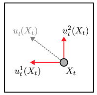
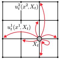
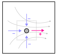
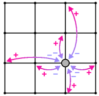
Flow $\Real^{N}$	Flow $[d]^{N}$	$\divv$ in $\Real^{N}$	$\divv$ in $[d]^{N}$

Figure 2: Discrete flow in $\gD=[d]^{N}$ here with $d=3,N=2$ (middle-left) versus continuous flow in $\Real^{N}$, $N=2$ (left). The rate of change of probability of a state (gray disk) is given by the divergence operator shown in the continuous case (middle right) and the discrete case (right).

2.4 Generating Probability Velocities

Continuous generating velocity. Sampling in continuous FM is performed by updating the current (continuous) sample $X_{t}\in\Real^{N}$, $t\in[0,1)$, according to a learned generating velocity field $u_{t}^{i}(X_{t})$, $i\in[N]$. Euler sampling follows the (deterministic) rule

$$X_{t+h}^{i}=X_{t}^{i}+hu_{t}^{i}(X_{t}),$$ (11)

where $h>0$ is a user-defined time step. Note that (11) is updating separately each of the sample coordinates, $X_{t}^{i}$, $i\in[N]$, see , Figure 2, left. The velocity $u_{t}^{i}(X_{t})$ can be either directly modeled with a neural network, or parameterized via the denoiser (a.k.a. $x$-prediction) or noise-prediction (a.k.a. $\eps$-prediction), see left column in Table 1. If, for all $t\in[0,1)$, starting at $X_{t}\sim p_{t}$ and sampling with (11) provides $X_{t+h}\sim p_{t+h}+o(h)$ then we say that $u_{t}$ generates $p_{t}$.

Generating probability velocity.

For defining FM in the discrete setting, we follow Campbell et al. (2024) and consider a Continuous-Time discrete Markov Chain (CTMC) paradigm, namely the sample $X_{t}$ is jumping between states in $\gD$, depending on a continuous time value $t\in[0,1]$. Similar to the continuous FM setting described above, we focus on a model that predicts the rate of probability change of the current sample $X_{t}$ in each of its $N$ tokens, see Figure 2, middle-left. Then, each token of the sample $X_{t}\sim p_{t}$ is updated independently by

$$X^{i}_{t+h}\sim\delta_{X^{i}_{t}}(\cdot)+hu_{t}^{i}(\cdot,X_{t}),$$ (12)

where we call $u_{t}$ the probability velocity as reminiscent of the velocity field in continuous Flow Matching, and as in the continuous case, we define:

Definition 2.1.

Probability velocity $u_{t}$ generates the probability path $p_{t}$ if, for all $t\in[0,1)$ and given a sample $X_{t}\sim p_{t}$, the sample $X_{t+h}$ defined in (12) satisfies $X_{t+h}\sim p_{t+h}+o(h)$.

Algorithm 1 formulates a basic sampling algorithm given a generating probability velocity $u_{t}$. In order for the r.h.s. of (12) to define a proper PMF for sufficiently small $h>0$, it is necessary and sufficient that the probability velocity satisfies the conditions

$$\sum_{x^{i}\in[d]}u_{t}^{i}(x^{i},z)=0,\text{ and }u_{t}^{i}(x^{i},z)\geq 0\text{ for all }i\in[N]\text{ and }x^{i}\neq z^{i}.\vspace{-3pt}$$ (13)

Algorithm 1 Flow Matching sampling.

velocity $u_{t}$, sample $X\sim p$, step size $h=\frac{1}{n}$

for $t=0,h,2h,\ldots,1-h$ do

     $X^{i}\sim\delta_{X^{i}}(\cdot)+hu^{i}_{t}(\cdot,X)$, for $i\in[N]$ $\triangleright$ eq. 24 or 22

end for

return $X$

Now the main question is how to find a probability velocity $u_{t}$ that generates the probability path defined in equations 7 and 8? A key insight in Flow Matching (Lipman et al., 2022) is that $u_{t}$ can be constructed as a marginalization of conditional probability velocities, $u_{t}^{i}(x^{i},z|x_{0},x_{1})$, generating the corresponding conditional probability paths $p_{t}(x^{i}|x_{0},x_{1})$. This can also be shown to hold in the discrete CTMC setting (Campbell et al., 2024), where a reformulation in our context and notation is as follows.

Theorem 2.2.

Given a conditional probability velocity $u_{t}^{i}(x^{i},z|x_{0},x_{1})$ generating a conditional probability path $p_{t}(x|x_{0},x_{1})$, the marginal velocity defined by

$$u_{t}^{i}(x^{i},z)=\sum_{x_{0},x_{1}\in\gD}u_{t}^{i}(x^{i},z|x_{0},x_{1})p_{t}(x_{0},x_{1}|z)$$ (14)

generates the marginal probability path $p_{t}(x)$, where by Bayes’ rule

$$p_{t}(x_{0},x_{1}|z)=\frac{p_{t}(z|x_{0},x_{1})\pi(x_{0},x_{1})}{p_{t}(x)}.$$ (15)

For completeness we provide a simple proof of this theorem in Section 10.2. The proof, similar to the continuous FM case, shows that $u_{t}$ and $p_{t}$ satisfy the (discrete version of the) Continuity Equation.

The Continuity Equation.

To provide the mathematical tool for showing that a probability velocity $u_{t}$ does indeed generate the probability path $p_{t}$, and also to further highlight the similarities to the continuous case, we next formulate the Kolmogorov Equations, which describe the state probability rate $\dot{p}_{t}(x)$, $x\in\gD$, in CTMC as a Continuity Equation (CE). The Continuity Equation, similarly to Kolmogorov Equations, describes $\dot{p}_{t}(x)$, $x\in\Real^{N}$ in the continuous case, and is formulated as the Partial Differential Equation (PDE)

$$\dot{p}_{t}(x)+\divv_{x}(p_{t}u_{t})=0,$$ (16)

where the divergence operator $\divv_{x}(v)$ applied to a vector field $v:\Real^{N}\too\Real^{N}$ is defined by

$$\divv_{x}(v)=\sum_{i=1}^{N}\partial_{x^{i}}v^{i}(x),$$ (17)

and intuitively means the total flux leaving $x$, see Figure 2 (middle-right). This gives an intuitive explanation to the Continuity Equation: the rate of the probability $\dot{p}_{t}(x)$ of a state $x\in\Real^{N}$ equals the total incoming probability flux, $p_{t}u_{t}$, at $x$. In the discrete case (CTMC) the Continuity Equation ((16)) holds as is, once the discrete divergence operator is properly defined, , to measure the outgoing flux from a discrete state. In more detail, given some vector field, which in the discrete case is a scalar-valued function over pairs of states, $v:\gD\times\gD\too\Real$, the discrete divergence is

$$\divv_{x}(v)=\sum_{z\in\gD}\brac{v(z,x)-v(x,z)},$$ (18)

where $v(z,x)$ represents the flux $x\too z$ and $v(x,z)$ represent the opposite flux $z\too x$; see Figure 2, right. Now, in our case (see Figure 2, middle-left), the probability flux at a state $x\in\gD$ involves all sequences with at most one token difference from $x$, , the probability flux $p_{t}u_{t}$ at $x$ takes the form $v(x,z)=p_{t}(z)u_{t}^{i}(x^{i},z)$ and $v(z,x)=p_{t}(x)u_{t}^{i}(z^{i},x)$ for $z$ and $x$ that differ only in the $i$-th token, $v(x,x)=\sum_{i=1}^{N}u_{t}^{i}(x^{i},x)$, and $v(x,z)=0$ for all other $(z,x)\in\gD\times\gD$. A direct calculation now shows (see Section 10.1):

$$\divv_{x}(p_{t}u_{t})=-\sum_{z\in\gD}p_{t}(z)\brac{\sum_{i=1}^{N}\delta_{z}(x^{\bar{i}})u_{t}^{i}(x^{i},z)}.$$ (19)

Checking that a probability velocity $u_{t}$ generates a probability path $p_{t}$ (in the sense of Definition 2.1) amounts to verifying the Continuity Equation ((16)). Indeed, using arguments from Campbell et al. (2024) and the discrete divergence operator, the PMF of $X_{t+h}$ defined by sampling according to (12) is

$$\E_{X_{t}}\prod_{i=1}^{N}\brac{\delta_{X_{t}}(x^{i})+hu_{t}^{i}(x^{i},X_{t})}=\E_{X_{t}}\brac{\delta_{X_{t}}(x)+h\sum_{i=1}^{N}\delta_{X_{t}}(x^{\bar{i}})u^{i}_{t}(x^{i},X_{t})}+o(h)$$ (20)

$$\qquad\quad=p_{t}(x)-h\divv_{x}(p_{t}u_{t})+o(h){\color[rgb]{1,0,0}\overset{(\ref{e:ce})}{=}}p_{t}(x)+h\dot{p}_{t}(x)+o(h)=p_{t+h}(x)+o(h),$$

where we assume $X_{t}\sim p_{t}$, the first equality uses the identity $\prod_{i}\brac{a^{i}+hb^{i}}=\prod_{i}a^{i}+h\sum_{i}(\prod_{j\neq i}a^{j})b^{i}+o(h)$, the second equality uses eq. 19, and the previous-to-last equality uses the Continuity Equation ((16)). This shows that if the Continuity Equation holds then $u_{t}$ generates $p_{t}$ in the sense of Definition 2.1.

Conditional and marginal generating velocities. We provide the probability velocities generating the conditional probability paths $p_{t}(x|x_{0},x_{1})$ defined in equations 7 and 8. Then, using the marginalization formula in (14) we end up with a closed-form marginal velocity for the probability paths $p_{t}(x)$. In Section 10.3 we show

Theorem 2.3 (Probability velocity of conditional paths).

A generating probability velocity for the conditional paths $p_{t}(x|x_{0},x_{1})$ defined in equations 7 and 8 is

$$u_{t}^{i}(x^{i},z|x_{0},x_{1})=\sum_{j=1}^{m}a_{t}^{i,j}w^{j}(x^{i}|x_{0},x_{1})+b_{t}^{i}\delta_{z}(x^{i}),$$ (21)

with $a_{t}^{i,j}=\dot{\kappa}_{t}^{i,j}-\kappa_{t}^{i,j}\dot{\kappa}_{t}^{i,\ell}/\kappa_{t}^{i,\ell}$, and $b_{t}^{i}=\dot{\kappa}_{t}^{i,\ell}/\kappa_{t}^{i,\ell}$ where $\ell=\argmin_{j\in[m]}\brac{\dot{\kappa}_{t}^{i,j}/\kappa_{t}^{i,j}}$.

Now, computing the marginal probability velocity using (14) applied to the conditional probability velocity in (21) gives

$$u^{i}_{t}(x^{i},z)=\sum_{j=1}^{m}a^{i,j}_{t}\hat{w}^{j}_{t}(x^{i},z)+b^{i,j}_{t}\delta_{z}(x^{i}),$$ (22)

where the posteriors $\hat{w}^{j}_{t}$ of $w^{j}$ (that are later shown to be tractable to learn) are defined by

$$\hat{w}_{t}^{j}(x^{i},z)=\sum_{x_{0},x_{1}\in\gD}w^{j}(x^{i}|x_{0},x_{1})p_{t}(x_{0},x_{1}|z),$$ (23)

where $p_{t}(x_{0},x_{1}|z)$ (defined in (15)) is the posterior probability of $x_{0},x_{1}$ conditioned on the current state $X_{t}=z$. A useful instantiation of the general velocity in (22) is when considering the path family in (9), for which $w^{1}(x^{i}|x_{0},x_{1})=\delta_{x_{1}}(x^{i})$, $w^{2}(x^{i}|x_{0},x_{1})=\delta_{x_{0}}(x^{i})$, $\kappa_{t}^{i,1}=\kappa_{t}$, $\kappa_{t}^{i,2}=1-\kappa_{t}$, $\dot{\kappa}_{t}\geq 0$ (, monotonically non-decreasing in $t$) and in this case (22) reads as

$$u^{i}_{t}(x^{i},z)=\frac{\dot{\kappa}_{t}}{1-\kappa_{t}}\brac{p_{1|t}(x^{i}|z)-\delta_{z}(x^{i})}$$ (24)

where we use the notation $p_{1|t}(x^{i}|X_{t})=\sum_{x_{0},x_{1}}\delta_{x_{1}}(x^{i})p_{t}(x_{0},x_{1}|X_{t})$ for the probability denoiser.

	Continuous Flow Matching	Discrete Flow Matching
Marginal prob.	$p_{t}(x)=\sum_{x_{0},x_{1}}\prod_{i=1}^{N}p_{t}(x^{i}|x_{0},x_{1})\pi(x_{0},x_{1})$
Conditional prob.	$p_{t}(x^{i}|x_{0},x_{1})=\delta_{\kappa_{t}x_{1}+(1-\kappa_{t})x_{0}}(x^{i})$	$p_{t}(x^{i}|x_{0},x_{1})=\kappa_{t}\delta_{x_{1}}(x^{i})+(1-\kappa_{t})\delta_{x_{0}}(x^{i})$
VF-Denoiser	$u^{i}_{t}(X_{t})=\frac{\dot{\kappa}_{t}}{1-\kappa_{t}}\brac{{\color[rgb]{0,0,1}{\hat{x}}^{i}_{1|t}(X_{t})}-X_{t}^{i}}$	$u^{i}_{t}(x^{i},X_{t})=\frac{\dot{\kappa}_{t}}{1-\kappa_{t}}\brac{{\color[rgb]{0,0,1}p_{1|t}(x^{i}|X_{t})}-\delta_{X_{t}}(x^{i})}$
VF-Noise-pred	$u^{i}_{t}(X_{t})=\frac{\dot{\kappa}_{t}}{\kappa_{t}}\brac{X^{i}_{t}-{\color[rgb]{1,0,0}{\hat{x}}^{i}_{0|t}(X_{t})}}$	$u^{i}_{t}(x^{i},X_{t})=\frac{\dot{\kappa}_{t}}{\kappa_{t}}\brac{\delta_{X_{t}}(x^{i})-{\color[rgb]{1,0,0}p_{0|t}(x^{i}|X_{t})}}$

Table 1: Generating (marginal) velocity fields have identical form for the continuous and discrete FM when using denoiser/noise-prediction parameterization; ${\color[rgb]{0,0,1}\hat{x}_{1|t}(z)}=\E_{X_{1}\sim p_{t}(\cdot|z)}X_{1}$ is the standard continuous denoiser (a.k.a. $x$-prediction) and ${\color[rgb]{1,0,0}\hat{x}_{0|t}(z)}=\E_{X_{0}\sim p_{t}(\cdot|z)}X_{0}$ is the standard noise-prediction (a.k.a. $\epsilon$-prediction).

Sampling backward in time.

We can also sample backwards in time by following the sampling rule $X_{t-h}^{i}\sim\delta_{X_{t}^{i}}(\cdot)-hu_{t}^{i}(\cdot,X_{t})$. In this case $-u_{t}^{i}(x^{i},z)$ should satisfy (13). A (backward-time) generating probability velocity can then be achieved from (22) with the simple change to the coefficients $a^{i,j}_{t}$ and $b^{i,j}_{t}$, see Section 10.4. For $p_{t}$ defined with (9) the generating velocity is

$$u^{i}_{t}(x^{i},z)=\frac{\dot{\kappa}_{t}}{\kappa_{t}}\brac{\delta_{z}(x^{i})-p_{0|t}(x^{i}|z)},$$ (25)

where in this case $p_{0|t}(x^{i}|z)=\sum_{x_{0},x_{1}\in\gD}\delta_{x_{0}}(x^{i})p_{t}(x_{0},x_{1}|z)$ is the probability noise-prediction.

Remarkably, the generating velocity fields in 24 and 25 take the exact same form as the generating (a.k.a. marginal) velocity fields in continuous flow matching when parameterized via the denoiser or noise-prediction parameterizations and using the same schedulers, see Table 1 and Section 10.9 for explanation of the continuous case. In Section 10.4 we provide the backward-time version of Theorem 2.3.

Corrector sampling.

Combining the forward-time $\hat{u}_{t}$ (eq. 24) and backward-time $\check{u}_{t}$ (eq. 25), ,

$$\bar{u}_{t}^{i}(x^{i},z)=\alpha_{t}\hat{u}_{t}^{i}(x^{i},z)-\beta_{t}\check{u}_{t}^{i}(x^{i},z),$$ (26)

provides a valid forward-time probability velocity field (, satisfies (13)) for $t\in(0,1)$ as long as $\alpha_{t},\beta_{t}>0$. This velocity field can be used for two types of corrector sampling: (i) When $\alpha_{t}-\beta_{t}=1$ sampling with $\bar{u}_{t}$ leads to corrector sampling where intuitively each step moves $1+\alpha_{t}$ forward in time and $-\alpha_{t}$ backwards, which allows reintroducing noise into the sampling process; and (ii) when $\alpha_{t}-\beta_{t}=0$ sampling with $\bar{u}_{t}$ when fixing $t\in(0,1)$ leads to corrector iterations where limit samples distribute according to $p_{t}$. In  Section 10.6 we prove:

Theorem 2.4.

For perfectly trained posteriors and $\alpha_{t},\beta_{t}>0$, $t\in(0,1)$, $\bar{u}_{t}$ in (26) is a probability velocity, , satisfies (13), and: (i) For $\alpha_{t}-\beta_{t}=1$, $\bar{u}_{t}$ provides a probability velocity generating $p_{t}$; (ii) For $\alpha_{t}-\beta_{t}=0$, repeatedly sampling with $\bar{u}_{t}$ at fixed $t\in(0,1)$ and sufficiently small $h$ is guaranteed to converge to a sample from $p_{t}$.

One simplification to (26) can be done in the case of paths constructed with conditional as in (9), independent coupling $\pi(x_{0},x_{1})=p(x_{0})q(x_{1})$, and i.i.d. source $p(x_{0})=\prod_{i=1}^{N}p(x_{0}^{i})$, , $p(x_{0}^{i})$ is uniform over $[d]$ or $\delta_{\dummy}(x_{0}^{i})$. In this case, the backward-time formula in (25) take an equivalent simpler form

$$\check{u}_{t}^{i}(x^{i},z)=\frac{\dot{\kappa}_{t}}{\kappa_{t}}\brac{\delta_{z}(x^{i})-p(x^{i})},$$ (27)

which does not require estimation of the posterior $p_{0|t}$. See Section 10.5 for the derivation.

Training.

Equation 22 shows that for generating samples from a probabilty path $p_{t}(x)$ we require the posteriors $\hat{w}_{t}^{j}(x^{i}|X_{t})$. Training such posteriors can be done by minimizing the loss

$$\gL(\theta)=-\sum_{j\in[m],i\in[N]}\E_{t,(X_{0},X_{1}),X_{t},Y_{j}^{i}}\log\hat{w}_{t}^{j}(Y_{j}^{i}|X_{t};\theta),$$ (28)

where $t$ is sampled according to some distribution in $[0,1]$ (we used uniform), $(X_{0},X_{1})\sim\pi(X_{0},X_{1})$, $X_{t}\sim p_{t}(X_{t}|X_{0},X_{1})$, and $Y_{j}^{i}\sim w^{j}(Y_{j}^{i}|X_{0},X_{1})$; $\theta\in\Real^{p}$ denotes the learnable parameters. In the common case we use in this paper of learning a single posterior, , the probability denoiser $p_{1|t}$, the loss takes the form $\gL(\theta)=-\sum_{i\in[N]}\E_{t,(X_{0},X_{1}),X_{t}}\log p_{1|t}(X_{1}^{i}|X_{t})$. In Section 10.7 we prove:

Proposition 2.5.

The minimizer of $\gL$ ((28)) is $\hat{w}_{t}^{j}(x^{i}|X_{t})$ ((23)).

lcccccc 4-6,6-6 9-10 Method NFE Llama-2$\downarrow$ Llama-3$\downarrow$ GPT2$\downarrow$ Entropy
Data - 7.0 9.4 14.7 7.7
Autoregressive 1024 31.4 54.8 45.3 7.1
Savinov et al. (2021)200 29.545.134.75.2
Austin et al. (2021a)1000 697.6 768.8 837.8 7.6
Han et al. (2022)$>$10000 73.3 203.1 99.2 4.8
Lou et al. (2023) 2565121024 38.633.727.269.258.643.964.353.440.57.87.77.6
Campbell et al. (2024) 2565121024 38.533.528.7 69.056.546.5 65.253.343.0 7.87.77.6
 ((9)) 2565121024 34.230.022.5 58.548.833.8 54.243.529.3 7.77.67.2
 ((10)) 2565121024 30.027.522.3 48.243.531.9 47.741.828.1 7.67.57.1

Table 2: Generative perplexity on unconditional text generation compared to prior work.

3 Related work

In the section we cover the most related work to ours; in Section 6 we cover other related work.

Discrete Flows (Campbell et al., 2024) is probably the most related work to ours. We build upon their CTMC framework and offer the following generalizations and simplifications over their original formulation: Campbell et al. (2024) define a rate matrix (equivalent to our probability velocity) for generation, expressed as an expectation over the posterior, $\E_{X_{1}^{i}\sim p_{1|t}(X_{1}^{i}|X_{t})}R_{t}^{*,i}(X_{t}^{i},x^{i}|X_{1}^{i})$ where $R^{*}$ is defined using the conditional probability path. This formulation requires computing an expectation during sampling in the general case (see their Algorithm 1) or a particular path-dependent derivation. We show, for a more general class of probability paths, there exists a unified formulation for the probability velocity in terms of the probability denoiser, , (24), or alternatively using other posteriors besides the denoiser allowing for backward-time sampling ((25)) or more elaborate path sampling ((22)). With the probability denoiser and noise-prediction we recreate the exact same formulas as the continuous Flow Matching counterpart. Furthermore, our sampling turns out to coincides with Campbell et al. (2024) for the case of linear schedulers, i.e., (8) with $\kappa_{t}=t$. However, in practice we observe that large gains in performance can be achieved by considering different paths during training and sampling. Our corrector term ((26)) also provides a unified general formula for both corrector iterations (Song et al., 2020; Campbell et al., 2022) and stochastic sampling of Campbell et al. (2024). Lastly, we opted for the term probability velocity for $u^{i}_{t}(x^{i},X_{t})$ as it is not precisely a rate matrix in the state space $\gD\times\gD$ used in CTMC since $u_{t}^{i}(x^{i},z)$ for all $i\in[N]$ define multiple self-edges $z\too z$.

Masked modeling (Ghazvininejad et al., 2019; Chang et al., 2022). In case of a masked model, , when the source distribution is $p(x)=\delta_{\dummy}(x)$, we achieve an interesting connection with MaskGit showing it is actually an instance of Discrete Flow Matching with a small yet crucial change to its sampling algorithm. First, in Section 10.8 we prove that in the masked setting, the probability denoiser $p_{1|t}$ is time-independent:

Proposition 3.1.

For paths defined by equations 7 and 9 with source $p(x)=\delta_{\dummy}(x)$ the posterior $p_{t}(x_{0},x_{1}|z)=p(x_{0},x_{1}|z)$ is time-independent. Consequently, the probability denoiser $p_{1|t}(x^{i}|z)=p_{1}(x^{i}|z)$ is also time-independent.

This shows that the probability denoiser can be learned with no time dependence, similar to the unmasking probabilities in MaskGit. During sampling however, there are two main differences between our sampling and MaskGit sampling. First, unmasking of tokens in our algorithm is done according to the probability $\delta_{X_{t}}(x^{i})+hu^{i}_{t}(x^{i},X_{t})$ independently for each token $x^{i}$, $i\in[N]$. This procedure is justified as it samples from the correct probability asymptotically via the derivation of the Continuity Equation 20. This is in contrast to MaskGit that prioritizes the token to be unmasked according to some confidence. In the experiments section we show that MaskGit’s prioritization, although has some benefit in the very low NFE regime, is actually introducing a strong bias in the sampling procedure and leads to inferior overall results. Secondly, using corrector sampling allows for reintroducing masks to already unmasked tokens in a way that is still guaranteed to produce samples from $p_{t}$, see Theorem 2.4; we find this to have a significant positive effect on the generation quality.

Discrete diffusion. D3PM (Austin et al., 2021a) and Argmax flows (Hoogeboom et al., 2021) introduced diffusion in discrete spaces by proposing a corruption process for categorical data. A later work by Campbell et al. (2022) introduced discrete diffusion models with continuous time, and Lou et al. (2023) proposed learning probability ratios, extending score matching (Song and Ermon, 2019) to discrete spaces.

lcccccc 5-6 6-7 Method Model Size NFE Llama-2$\downarrow$ Llama-3$\downarrow$ Entropy
Llama-3 (Reference) 8B 512 6.4 7.3 6.8
Llama-2 (Reference) 7B 512 5.3 8.3 7.1
Autoregressive 1.7B 512 14.3 22.3 7.2
Savinov et al. (2021) 1.7B 200 10.8 15.4 4.7
 (U-coupling) 1.7B 25651210.79.5 11.210.3 6.76.7
 (C-coupling) 1.7B 256512 10.28.9 10.09.7 6.86.7

Table 3: Generative perplexity on conditional text generation.

llcccccc 5-7 Method Data HumanEval$\uparrow$ MBPP (1-shot)$\uparrow$
Pass@1 Pass@10 Pass@25 Pass@1 Pass@10 Pass@25
Autoregressive Text 1.2 3.1 4.8 0.2 1.7 3.3
Code 14.3 21.3 27.8 17.0 34.3 44.1
Text 1.2 2.6 4.0 0.4 1.1 3.6
Code 6.7 13.4 18.0 6.7 20.6 26.5
 (Oracle length)Code 11.6 18.3 20.6 13.1 28.4 34.2

Table 4: Execution based code generation evaluation.

4 Experiments

We evaluate our method on the tasks of language modeling, code generation, and image generation. For language modeling, we compare the proposed method against prior work considering the widely used generative perplexity metric. We scale the models to 1.7 billion parameters and present results on coding tasks, i.e., HumanEval (Chen et al., 2021), MBPP (Austin et al., 2021b), demonstrating the most promising results to date in a non-autoregressive context. In image generation, we present results for a fully discrete CIFAR10 (Krizhevsky et al., 2009). Further details of the experimental setup for each model are provided in Section 12.

Experimental setup. In our experiments we used the masked source, , $p=\delta_{\dummy}$, and trained with both unconditional coupling (U-coupling, (4)) and conditional couplings (C-coupling, (5)) with the probability path defined in equations 7, 9 and in one case 10. We trained a probability denoiser (loss in (28)) and sampled using the generating velocity in (24) and Algorithm 1. We used a particular choice of probability path scheduler $\kappa_{t}$, as well as corrector steps defined by a scheduler $\alpha_{t}$ and temperature annealing. We found the choice of these schedulers to be pivotal for the model’s performance. In Section 9 we perform an ablation study, evaluating various scheduler choices.

4.1 Language modeling

We experimented with our method in three settings: (i) Small model (150M parameters) - comparison to other non-autoregressive baselines in unconditional text generation; (ii) Large model (1.7B parameters) - comparison to autoregressive models in conditional text generation; and (iii) Large model (1.7B parameters) - conditional code generation. As computing exact likelihood for non-autoregressive model is a challenge, for (i),(ii) we use the generative perplexity metric (Section 12 measured with GPT2 (Radford et al., 2019), Llama-2 (Touvron et al., 2023), and Llama-3, and we also monitor the sentence entropy (Section 12) to measure diversity of tokens and flag repetitive sequences, which typically yield low perplexity. Throughout our experiments we noticed entropy $\geq 6$ usually corresponds to diverse texts. For (iii) we evaluated using the success rate of coding tasks.

Evaluation against prior work. We evaluate our method against prior work on non-autoregressive modeling. For a fair comparison, all methods are trained on a 150M parameters models using the OpenWebText (Gokaslan and Cohen, 2019) dataset. We also fix all sampling hyperparameters to the most basic settings, , no temperature, top probability, corrector steps, etc. For our method we tried two paths defined by equations 9 and 10. Results are reported in Section 2.4, where our method outperforms all baselines in generative perplexity for all numbers of function evaluations (NFE).

Conditional text generation. In this experiment, we train both C-coupling and U-coupling 1.7B parameters  models with paths defined by (9) on a large scale data mix (Touvron et al., 2023). Section 3 presents the generative perplexity of conditional generations from our method; the conditions we used are the prefixes of the first 1000 samples in OpenWeb dataset. We also compare to existing state-of-the-art autoregressive models. Our results demonstrate that our model effectively narrows the gap in generative perplexity with autoregressive models, while maintaining an entropy comparable to the recent Llama-3 8B model. Furthermore, we note the C-coupling trained model produces slightly better perplexity in conditional tasks than the U-coupling model. In Section 14 we present qualitative conditional samples produced by our U-coupling model.

Code generation. Here we trained our basic setting of a 1.7B parameters  model with U-coupling and path as in (9) on a code-focused data mix (Roziere et al., 2023). Section 3 presents results on HumanEval and MBPP (1-shot) for pass@$\{1,10,25\}$. In Section 3, ‘Oracle length’ evaluates the performance of our model when conditioning on the length of the solution. This is done by inserting an ‘end of text’ token in the same position of the ground truth solution. Our method achieves non-trivial results on both tasks, which to the best of our knowledge is the first instance of a non-autoregressive method being capable of non-trivial coding tasks. In Section 8, we analyze the proposed method for code infilling, which can be achieved as our model allows non-autoregressive generation. Lastly, in Section 13 we show qualitative examples of success and failure cases produced by our model on the coding tasks, and in Section 13.3 we show examples of code infilling.

4.2 Image generation

Figure 3: FID vs. NFE on CIFAR10.

We performed a fully discrete image generation, without using any metric or neighboring information between color values. We trained an  model with U-coupling and path as in (9) on CIFAR10 to predict discrete color value for tokens, , $d=256$, with sequence length of $N=32\times 32\times 3$. For generative quality we evaluate the Fréchet Inception Distance (FID) (Heusel et al., 2017). Ablations for the probability path schedulers are provided in Figure 8 in the Section 12. In Figure 3 we compare our method with: (i) MaskGIT (Chang et al., 2022); and (ii) (Campbell et al., 2024) which coincides with our method for a linear scheduler. More details in Section 12. As can be seen in the Figure 3, our method outperforms both baselines, achieving $3.63$ FID at $1024$ NFE. As discussed above, MaskGit sampling performs better for low NFE but quickly deteriorates for higher NFE. We attribute this to a bias introduced in the sampling process via the confidence mechanism.

5 Conclusions and future work

We introduce Discrete Flow Matching, a generalization of continuous flow matching and discrete flows that provides a large design space of discrete non-autoregressive generative models. Searching within this space we were able to train large scale language models that produce generated text with an improved generative perplexity compared to current non-autoregressive methods and able to solve coding tasks at rates not achievable before with non-autoregressive models, as far as we are aware. While reducing the number of network evaluations required to generate a discrete sample compared to autoregressive models, Discrete FM still does not achieve the level of sampling efficiency achieved by its continuous counterpart, flagging an interesting future work direction. Another interesting direction is to explore the space of probability paths in (8) (or a generalization of which) beyond what we have done in this paper. We believe discrete non-autoregressive models have the potential to close the gap and even surpass autoregressive models as well as unlock novel applications and use cases. As our work introduces an alternative modeling paradigm to discrete sequential data such as language and code, we feel it does not introduce significant societal risks beyond those that already exist with previous large language models.

6 Related works, continuation

We provide here some more details on relevant related works.

Continuous diffusion and flows.

Another line of works has been exploring the use of continuous space diffusion for discrete data, typically operating in the logits space (Dieleman et al., 2022; Li et al., 2022; Han et al., 2022; Lin et al., 2022; Chen et al., 2022). An additional body of work has been focusing on the adoption of latent diffusion-like modeling (Lovelace et al., 2022; He et al., 2022). Stark et al. (2024) proposed to learn a continuous Flow Matching on the probability simplex with Dirichlet paths.

Autoregressive modeling.

Autoregressive models have been a significant area of focus in recent years, particularly in the context of natural language processing and machine learning (Zhao et al., 2023). Autoregressive modeling, in its most fundamental form, utilizes the chain rule to learn the joint sequence probability by breaking it down into next-token conditional probabilities. GPT-2 (Radford et al., 2019), showcased the power of autoregressive language models in generating coherent and contextually relevant text over long passages. Its successor, GPT-3 (Brown et al., 2020), further pushed the boundaries, demonstrating impressive performance across a range of tasks without task-specific training data. Later models were adapted to other domains such as, code (Roziere et al., 2023; Li et al., 2023; Chen et al., 2021), biology (Zhang et al., 2024; Ferruz and Höcker, 2022; Madani et al., 2023), math (Romera-Paredes et al., 2024; Imani et al., 2023; Ahn et al., 2024), audio (Kreuk et al., 2022; Copet et al., 2024; Hassid et al., 2024) and more.

Masked generative modeling.

Masked generative modeling proposes to mask a variable portion of the input sequence and training a model to predict this masked section.  Ghazvininejad et al. (2019) proposed Mask-Predict, a masked language modeling with parallel decoding.  Savinov et al. (2021) extended the mask-modeling approach by employing an additional loss term that incorporates rolling model predictions. MaskGIT (Chang et al., 2022) followed a similar path, for the task of class-conditioned image synthesis,  Chang et al. (2023) extended this approach to high-quality textually guided image generation over low-resolution images followed by a super-resolution module. Recently, Ziv et al. (2024) proposed a text-to-music method, which relies on the MaskGIT foundations while observing that span masking boosts the quality of the generated sequence significantly.

7 Further implementation details

Safe sampling.

When sampling according to Algorithm 1 using the generating probability velocity in (22), an arbitrary step size $h>0$ can make some probabilities in $\delta_{X_{t}^{i}}(\cdot)+hu_{t}^{i}(\cdot,X_{t})$ negative and consequently require clamping and injecting further error into the sampling process that can in turn accumulate to a non-negligible global sampling error. A simple fix that guarantees a valid probability distribution while keeping the $o(h)$ sampling error at the relatively manageable price of potentially more function evaluations is using the following adaptive step size in Algorithm 1: at time $t\in[0,1)$ use

$$h_{\text{\tiny adaptive}}=\min\set{h,\min_{i}\abs{\frac{\kappa_{t}^{i,\ell}}{\dot{\kappa}_{t}^{i,\ell}}}}.$$ (29)

As can be verified with the general probability velocity formula in (22), the above choice for $h_{\text{\tiny adaptive}}$ guarantees $\delta_{X_{t}^{i}}(\cdot)+hu_{t}^{i}(\cdot,X_{t})$ is a valid PMF. As mostly used in this paper, for the probability denoiser parameterization ((24)) the adaptive step is

$$h_{\text{\tiny adaptive}}=\min\set{h,\frac{1-\kappa_{t}}{\dot{\kappa}_{t}}}.$$ (30)

With the corrector sampling (equations 26 and 51) we have the adaptive step:

$$h_{\text{\tiny adaptive}}=\min\set{h,\brac{\frac{\alpha_{t}\dot{\kappa}_{t}}{1-\kappa_{t}}+\frac{\beta_{t}\dot{\kappa}_{t}}{\kappa_{t}}}^{-1}}.$$ (31)

Conditioning.

In our unconditional coupling (U-coupling), see (5), we define the conditioning pattern based on prefixes of random length $N_{0}<N$, ,

$$\sI=(\overbrace{1,\ldots,1}^{N_{0}},\overbrace{0,\ldots,0}^{N-N_{0}}).$$

During the training phase, we sample $N_{0}\sim\mathcal{U}(0,N)$ and adjust the input sequence in accordance with the mask $\sI$.

During conditional sampling with Algorithm 1 we replace, after each update step, the relevant tokens with the conditioned ones, , $\tilde{X}=\sI\odot Y+(\one-\sI)\odot X$, where $X$ is the current sample, $Y$ is the condition, and $\sI$ is the condition’s mask.

NFE bound.

For mask modeling, , $p=\delta_{\dummy}$, we have seen that the probability denoiser is time-independent (see Proposition 3.1). Consequently, when sampling with Algorithm 1 and $u_{t}$ from (24) without corrector sampling one is not required to recompute the forward pass $p_{1|t}(\cdot|X_{t})$ if $X_{t}$ is identical to $X_{t-h}$ (, no $\dummy$ has been unmasked). This means that the NFE of Algorithm 1 in this case is bounded by the number of tokens $N$.

Post training scheduler change.

For a trained posterior $\hat{w}_{t}(x^{i}|z)$ of a conditional probability path as in (9) with a scheduler $\kappa_{t}$, the velocity is given by equations 24 or 25, where $\hat{w}_{t}(x^{i}|z)$ is either $p_{1|t}(x^{i}|z)$ or $p_{0|t}(x^{i}|z)$ respectively. In this case, we can apply the velocities in equations 24 and 25 for sampling with any scheduler $\kappa^{\prime}_{t}$, using the change of scheduler formula for posteriors,

$$\hat{w}_{t}^{\prime}(x^{i}|z)=\hat{w}_{t^{\prime}}(x^{i}|z),$$ (32)

where $\hat{w}^{\prime}_{t}(x^{i}|z)$, is the posterior of the scheduler $\kappa^{\prime}_{t}$, $t^{\prime}=\kappa^{-1}_{\kappa^{\prime}_{t}}$, and $\kappa^{-1}$ is the inverse of $\kappa$. The scheduler change formula in (32) is proved in Proposition 10.8. We note that by Proposition 3.1, for mask modeling, , $p=\delta_{\dummy}$, the posterior $\hat{w}_{t}(x^{i}|z)$ is time independent. Hence, in that case, the posterior is not affected by a scheduler change.

8 Code infilling

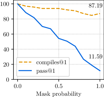
Figure 4: Pass@1 and compiles@1 scores for the 1.5B parameter models as a function of the input masking rations on HumanEval.

We additionally evaluate the proposed method considering the task of code infilling. In which, we are provided with an input prompt that contains various spans of masked tokens, and our goal is to predict them based on the unmasked ones. See Figure 1 (middle and right sub-figures) for a visual example. Notice, this evaluation setup is the most similar to the training process.

For that, we randomly mask tokens with respect to several masking rations, $p\in\{0.0,0.1,0.2,\dots,1.0\}$, from HumanEval and report both pass@1 and compiles@1 metrics. For the purpose of this analysis, we provide the oracle length for each masked span. In other words, the model predicts the masked tokens for already given maks length. Results for the 1.5B parameters models can be seen in Figure 4. As expected, both pass@1 and compiles@1 keep improving as we decrease the level of input masking. Interestingly, when considering the fully masked sequence, providing the oracle prediction length significantly improves the pass@1 scores (6.7 vs. 11.6).

9 Ablations

(a) Path scheduler, cubic poly.

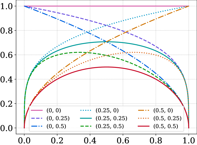
(b) Corrector scheduler $t^{a}(1-t)^{b}$.

(c) Temperature scheduler $(1-t)^{a}$.

Train and sampling path scheduler choice ($\kappa_{t}$).

We study how the choice of the probability path scheduler affects the model performance. For that, we consider a parametric family of cubic polynomial with parameters $a,b$:

$$\kappa_{t}\triangleq-2t^{3}+3t^{2}+a(t^{3}-2t^{2}+t)+b(t^{3}-t^{2}).$$ (33)

Note that $\kappa_{0}=0$ and $\kappa_{1}=0$ and $a$ and $b$ are setting the derivative of $\kappa_{t}$ at $t=0$ and $t=1$, respectively. We visualize this $\kappa_{t}$ with choices of $a,b\in\{0,1,2\}$ in Figure 5(a).

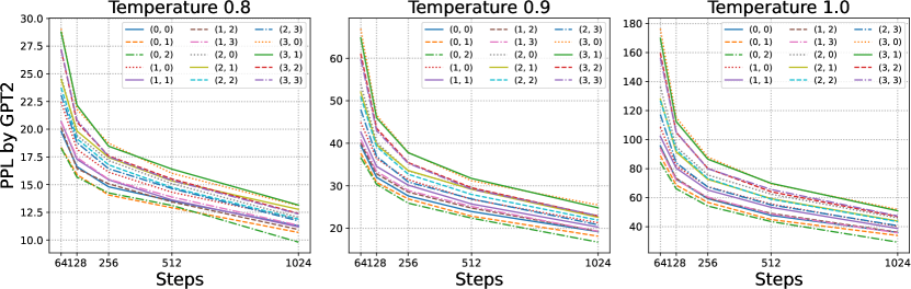
Figure 6: Path scheduler choice during training using various of constant temperature values.

To test the effect of path schedulers in training we have trained 150M parameters models for all choices of $a,b\in\{0,1,2,3\}$. We then generate 1000 samples from each model. The samples are computed using Algorithm 1 with the path scheduler the model was trained on, and with temperature levels $\tau\in\{0.8,0.9,1\}$, where temperature is applied via

$$p^{\tau}_{1|t}(x^{i}|X_{t})=\tau^{-1}\log p_{1|t}(x^{i}|X_{t}).$$ (34)

We then evaluate the generative perplexity of these samples with GPT-2. Figure 6 shows the results. The graphs indicate that, in the context of text modality, the cubic polynomial scheduler with $a\equiv 0,b\equiv 2$ (equivalent to a square function) achieves the highest performance. Consequently, we exclusively used this scheduler for the language models.

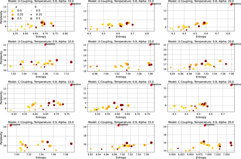
Figure 7: Corrector scheduler ablation.

Corrector scheduler.

In our experiments we only applied corrector sampling to our large models (U-coupling and C-coupling; 1.7B parameters). We used the optimal path schedulers from previous section and considered the following parametric family of schedulers for the corrector sampling:

$$\alpha_{t}=1+\alpha t^{a}(1-t)^{b},$$ (35)

where, we set $\beta_{t}=\alpha_{t}-1$ and generate 1000 samples using Algorithm 1 with parameter values $a,b\in\set{0,0.25,0.5}$ and $\alpha\in\set{10,15,20}$. We then evaluated generative perplexity for these samples with Llama-2, showing results in Figure 7. These plots indicate that smaller values of $a$ and $b$ result in lower perplexity values, albeit with somewhat reduced entropy. We therefore opted for setting $a=b=0.25$ that strikes a good balance between perplexity and entropy.

Temperature scheduling.

For temperature sampling, we consider the following scheduler:

$$\tau_{t}=\tau(1-t)^{2}.$$ (36)

10 Theory and proofs

10.1 Computation of the discrete divergence

We present the computation of the discrete divergence in (18), ,

$$\divv_{x}(p_{t}u_{t})=-\sum_{z\in\gD}p_{t}(z)\brac{\sum_{i=1}^{N}\delta_{z}(x^{\bar{i}})u_{t}^{i}(x^{i},z)}.$$ (37)

Computing the discrete divergence ((18)) of the flux $p_{t}u_{t}$ at a state $x$ amounts to adding outgoing flux from $x$ and subtracting the incoming flux into $x$. Using the fact that $\delta_{z}(x^{\bar{i}})=1$ if and only if $z=x$ or $z$ differs from $x$ only at the $i$-th token, gives:

$$\divv_{x}(p_{t}u_{t}) =\sum_{z\in\gD}\sum_{i=1}^{N}\delta_{x}(z^{\bar{i}})\parr$$

$$=p_{t}(x)\sum_{i=1}^{N}\sum_{z^{i}}{\color[rgb]{1,0,0}\overbrace{\brac{\sum_{z^{\bar{i}}}\delta_{x}(z^{\bar{i}})}}^{=1}}u^{i}_{t}(z^{i},x)-\sum_{z\in\gD}\sum_{i=1}^{N}\delta_{x}(z^{\bar{i}})p_{t}(z)u_{t}^{i}(x^{i},z)$$

$$=p_{t}(x)\sum_{i=1}^{N}{\color[rgb]{1,0,0}\overbrace{\brac{\sum_{z^{i}}u^{i}_{t}(z^{i},x)}}^{=0}}-\sum_{z\in\gD}\sum_{i=1}^{N}\delta_{x}(z^{\bar{i}})p_{t}(z)u_{t}^{i}(x^{i},z)\text{{\color[rgb]{0,0,0}\qquad\hfill$\triangleright$ \eqref{e:rate_conds}}}$$

$$=-\sum_{z\in\gD}\sum_{i=1}^{N}\delta_{x}(z^{\bar{i}})p_{t}(z)u_{t}^{i}(x^{i},z),$$

that gives (37) after noting that $\delta_{x}(z^{\bar{i}})=\delta_{z}(x^{\bar{i}})$.

10.2 Conditional velocities lead to marginal velocities

We provide a simple proof for Theorem 2.2, originally proved in (Campbell et al., 2024): thm:cond_to_marginal Given a conditional probability velocity $u_{t}^{i}(x^{i},X_{t}|x_{0},x_{1})$ generating a conditional probability path $p_{t}(x|x_{0},x_{1})$, the marginal velocity defined by

$$u_{t}^{i}(x^{i},X_{t})=\sum_{x_{0},x_{1}\in\gD}u_{t}^{i}(x^{i},X_{t}|x_{0},x_{1})p_{t}(x_{0},x_{1}|X_{t}),$$ (38)

generates the marginal probability path $p_{t}(x)$, where by Bayes’ rule

$$p_{t}(x_{0},x_{1}|X_{t})=\frac{p_{t}(X_{t}|x_{0},x_{1})\pi(x_{0},x_{1})}{p_{t}(x)}.$$ (39)

Proof 10.1 (Proof (Theorem 2.2)).

We start by taking the time derivative of the marginal probability path, $p_{t}(x)=\sum_{x_{0},x_{1}}p_{t}(x^{i}|x_{0},x_{1})\pi(x_{0},x_{1})$, as follows,

$$\dot{p}_{t}(x) =\sum_{x_{0},x_{1}}\dot{p}_{t}(x|x_{0},x_{1})\pi(x_{0},x_{1})$$

$$=\sum_{x_{0},x_{1}}\parr{\sum_{z}p_{t}(z|x_{0},x_{1})\brac{\sum_{i=1}^{N}\delta_{z}(x^{\bar{i}})u_{t}^{i}(x^{i},z|x_{0},x_{1})}}\pi(x_{0},x_{1})\text{{\color[rgb]{0,0,0}\qquad\hfill$\triangleright$ Continuity Equation (\ref{e:ce})}}$$

$$=\sum_{z}{\color[rgb]{0,0,1}p_{t}(z)}\brac{\sum_{i=1}^{N}\delta_{z}(x^{\bar{i}})\parr{\sum_{x_{0},x_{1}}u_{t}^{i}(x^{i},z|x_{0},x_{1})\frac{p_{t}(z|x_{0},x_{1})\pi(x_{0},x_{1})}{{\color[rgb]{0,0,1}p_{t}(z)}}}}$$

$$=\sum_{z}p_{t}(z)\brac{\sum_{i=1}^{N}\delta_{z}(x^{\bar{i}})u_{t}^{i}(x^{i},z)}$$

$$=-\divv_{x}(p_{t}u_{t})$$

Now since $u_{t}^{i}(x^{i},z)$ is a convex combinations of $u_{t}^{i}(x^{i},z|x_{0},x_{1})$ and these satisfy (13) then also $u_{t}^{i}(x^{i},X_{t})$ satisfies (13).

10.3 Probability velocities generating conditional probability paths

Equation 22 with the coefficients $a^{i,j}_{t}$ and $b^{i}_{t}$ are provided below,

$$u^{i}_{t}(x^{i},X_{t}|x_{0},x_{1})=\sum_{j=1}^{m}{\color[rgb]{0,0,1}\overbrace{\brac{\dot{\kappa}_{t}^{i,j}-\kappa_{t}^{i,j}\frac{\dot{\kappa}_{t}^{i,\ell}}{\kappa_{t}^{i,\ell}}}}^{{\color[rgb]{0,0,0}a^{i,j}_{t}}}}w^{j}(x^{i}|x_{0},x_{1})+{\color[rgb]{0,0,1}\overbrace{\brac{\frac{\dot{\kappa}_{t}^{i,\ell}}{\kappa_{t}^{i,\ell}}}}^{{\color[rgb]{0,0,0}b^{i}_{t}}}}\delta_{X_{t}}(x^{i}),$$ (40)

where

$$\ell=\ell(i,t)\defe\argmin_{j\in[m]}\brac{\dot{\kappa}_{t}^{i,j}/\kappa_{t}^{i,j}}.$$ (41)

thm:pvf_of_p_t_cond [Probability velocity of conditional paths] A generating probability velocity for the conditional paths $p_{t}(x|x_{0},x_{1})$ defined in equations 7 and 8 is

$$u_{t}^{i}(x^{i},X_{t}|x_{0},x_{1})=\sum_{j=1}^{m}a_{t}^{i,j}w^{j}(x^{i}|x_{0},x_{1})+b_{t}^{i}\delta_{X_{t}}(x^{i}),$$ (42)

with $a_{t}^{i,j}=\dot{\kappa}_{t}^{i,j}-\kappa_{t}^{i,j}\dot{\kappa}_{t}^{i,\ell}/\kappa_{t}^{i,\ell}$, and $b_{t}^{i}=\dot{\kappa}_{t}^{i,\ell}/\kappa_{t}^{i,\ell}$ where $\ell=\argmin_{j\in[m]}\brac{\dot{\kappa}_{t}^{i,j}/\kappa_{t}^{i,j}}$.

Proof 10.2 (Proof (Theorem 2.3)).

First, let us show that (40) satisfies the conditions in (13): Fix $X_{t}\in\gD$, and

$$\sum_{x^{i}}u^{i}_{t}(x^{i},X_{t}|x_{0},x_{1}) =\sum_{x^{i}}\brac{\sum_{j=1}^{m}\brac{\dot{\kappa}_{t}^{i,j}-\kappa_{t}^{i,j}\frac{\dot{\kappa}_{t}^{i,\ell}}{\kappa_{t}^{i,\ell}}}{w}^{j}(x^{i}|x_{0},x_{1})+\frac{\dot{\kappa}_{t}^{i,\ell}}{\kappa_{t}^{i,\ell}}\delta_{X_{t}}(x^{i})}$$

$$=\sum_{j=1}^{m}\brac{\dot{\kappa}_{t}^{i,j}-\kappa_{t}^{i,j}\frac{\dot{\kappa}_{t}^{i,\ell}}{\kappa_{t}^{i,\ell}}}+\frac{\dot{\kappa}_{t}^{i,\ell}}{\kappa_{t}^{i,\ell}}$$

$$=\sum_{j=1}^{m}\dot{\kappa}^{i,j}_{t}+\frac{\dot{\kappa}_{t}^{i,\ell}}{\kappa_{t}^{i,\ell}}\parr{1-\sum_{j=1}^{m}\kappa_{t}^{i,j}}\text{{\color[rgb]{0,0,0}\qquad\qquad\quad\hfill$\triangleright$ $\sum_{j}\kappa_{t}^{i,j}=1$, and $\sum_{j}\dot{\kappa}_{t}^{i,j}=0$}}$$

$$=0.$$

and for $x^{i}\neq X_{t}^{i}$ we have

$$u_{t}^{i}(x^{i},X_{t}|x_{0},x_{1})=\sum_{j=1}^{m}\brac{\frac{\dot{\kappa}_{t}^{i,j}}{\kappa_{t}^{i,j}}-\frac{\dot{\kappa}_{t}^{i,\ell}}{\kappa_{t}^{i,\ell}}}\kappa_{t}^{i,j}{w}^{j}(x^{i}|x_{0},x_{1})\geq 0$$ (43)

since $\kappa_{t}^{i,j}\geq 0$, $\hat{w}_{t}(x^{i}|z)\geq 0$, and $\frac{\dot{\kappa}_{t}^{i,j}}{\kappa_{t}^{i,j}}-\frac{\dot{\kappa}_{t}^{i,\ell}}{\kappa_{t}^{i,\ell}}\geq 0$ since $\ell=\argmin_{j\in[m]}\frac{\dot{\kappa}_{t}^{i,j}}{\kappa_{t}^{i,j}}$. Second, we show that $u_{t}$ satisfies the Continuity Equation ((16)). To that end we write (8) as

$$w^{\ell}(x^{i}|x_{0},x_{1})=\frac{1}{\kappa_{t}^{i,\ell}}\brac{p_{t}(x^{i}|x_{0},x_{1})-\sum_{j\neq\ell}\kappa_{t}^{i,j}w^{j}(x^{i}|x_{0},x_{1})},$$ (44)

where $\ell=\argmin_{j\in[m]}\frac{\dot{\kappa}_{t}^{i,j}}{\kappa_{t}^{i,j}}$. Now by differentiating $p_{t}(x|x_{0},x_{1})$ we get

$$p_{t}(x|x_{0},x_{1}) =\prod_{i=1}^{N}p_{t}(x^{i}|x_{0},x_{1})$$

$$\dot{p}_{t}(x|x_{0},x_{1}) =\sum_{i=1}^{N}p_{t}(x^{\bar{i}}|x_{0},x_{1})\dot{p}_{t}(x^{i}|x_{0},x_{1})$$

$$=\sum_{i=1}^{N}p_{t}(x^{\bar{i}}|x_{0},x_{1})\brac{\sum_{j=1}^{m}\dot{\kappa}_{t}^{i,j}w^{j}(x^{i}|x_{0},x_{1})}$$

$$=\sum_{i=1}^{N}p_{t}(x^{\bar{i}}|x_{0},x_{1})\brac{\sum_{j\neq\ell}\dot{\kappa}_{t}^{i,j}w^{j}(x^{i}|x_{0},x_{1})+\dot{\kappa}_{t}^{i,\ell}w^{\ell}(x^{i}|x_{0},x_{1})}$$

$$=\sum_{i=1}^{N}p_{t}(x^{\bar{i}}|x_{0},x_{1})\brac{\sum_{j=1}^{m}{\color[rgb]{1,0,0}\overbrace{{\color[rgb]{0,0,0}\brac{\dot{\kappa}_{t}^{i,j}-\kappa_{t}^{i,j}\frac{\dot{\kappa}_{t}^{i,\ell}}{\kappa_{t}^{i,\ell}}}}}^{a_{t}^{i,j}}}w^{j}(x^{i}|x_{0},x_{1})+{\color[rgb]{1,0,0}\overbrace{{\color[rgb]{0,0,0}\frac{\dot{\kappa}_{t}^{i,\ell}}{\kappa_{t}^{i,\ell}}}}^{b_{t}^{i}}}p_{t}(x^{i}|x_{0},x_{1})}\text{{\color[rgb]{0,0,0}\qquad\hfill$\triangleright$ \eqref{ae:w_ell_cond}}}$$

$$=\sum_{i=1}^{N}\brac{\sum_{j=1}^{m}a_{t}^{i,j}{\color[rgb]{1,0,0}\overbrace{{\color[rgb]{0,0,0}\brac{\sum_{z}\delta_{x}(z^{\bar{i}})p_{t}(z|x_{0},x_{1})}}}^{=p_{t}(x^{\bar{i}}|x_{0},x_{1})}}w^{j}(x^{i}|x_{0},x_{1})+b_{t}^{i}{\color[rgb]{1,0,0}\overbrace{{\color[rgb]{0,0,0}\brac{\sum_{z}\delta_{x}(z^{\bar{i}})\delta_{x}(z^{i})p_{t}(z|x_{0},x_{1})}}}^{=p_{t}(x|x_{0},x_{1})}}}$$

$$=\sum_{z}{\color[rgb]{0,0,1}p_{t}(z|x_{0},x_{1})}\sum_{i=1}^{N}\delta_{x}(z^{\bar{i}}){\color[rgb]{1,0,0}\overbrace{{\color[rgb]{0,0,0}\brac{\sum_{j=1}^{m}a_{t}^{i,j}w^{j}(x^{i}|x_{0},x_{1})+b_{t}^{i}\delta_{x}(z^{i})}}}^{u_{t}^{i}(x^{i},z|x_{0},x_{1})}}\quad\text{{\color[rgb]{0,0,0}\hfill$\triangleright$ $\delta_{x}(z^{i})=\delta_{z}(x^{i}),\ \delta_{x}(z^{\bar{i}})=\delta_{z}(x^{\bar{i}})$}}$$

$$=-\divv_{x}(p_{t}(\cdot|x_{0},x_{1})u_{t}(\cdot|x_{0},x_{1})),$$

as required.

10.4 Backward-time generating probability velocity.

Here we prove the equivalent of Theorem 2.3 for backward-time generating probability field. But first, let us justify the backward sampling formula,

$$X_{t-h}^{i}\sim\delta_{X_{t}^{i}}(\cdot)-hu_{t}^{i}(\cdot,X_{t}).$$ (45)

Similar to (20) we have

$$\E_{X_{t}}\prod_{i=1}^{N}\brac{\delta_{X_{t}}(x^{i})-hu_{t}^{i}(x^{i},X_{t})}=\E_{X_{t}}\brac{\delta_{X_{t}}(x)-h\sum_{i=1}^{N}\delta_{X_{t}}(x^{\bar{i}})u^{i}_{t}(x^{i},X_{t})}+o(h)$$

$$\qquad\quad=p_{t}(x)+h\divv_{x}(p_{t}u_{t})+o(h){\color[rgb]{1,0,0}\overset{(\ref{e:ce})}{=}}p_{t}(x)-h\dot{p}_{t}(x)+o(h)=p_{t-h}(x)+o(h).$$

Therefore if the Continuity equation holds and $-u_{t}$ satisfies the conditions in (13) then given $X_{t}\sim p_{t}$, (45) provides an approximation $X_{t-h}\sim p_{t-h}+o(h)$. The change to the generating probability velocity in (22) to accommodate reverse time sampling is to replace the argmin in (41) with argmax,

$$\ell=\ell(i,t)\triangleq\argmax_{j\in[m]}\brac{\dot{\kappa}_{t}^{i,j}/\kappa_{t}^{i,j}}.$$ (46)

An analogous result to Theorem 2.3 for backward-time sampling is therefore,

Theorem 10.3 (Probability velocity of conditional paths, backward time).

The probability velocity $-u_{t}$, where $u_{t}$ defined in (21) with $\ell=\argmax_{j\in[m]}\brac{\dot{\kappa}_{t}^{i,j}/\kappa_{t}^{i,j}}$ is a backward-time generating probability velocity for the conditional paths $p_{t}(x|x_{0},x_{1})$ defined in equations 7 and 8.

Proof 10.4.

We follow the proof of Theorem 2.3 and indicate the relevant changes. First, for arbitrary $X_{t}\in\gD$,

$$\sum_{x^{i}}u_{t}^{i}(x^{i},X_{t})=0,$$ (47)

exactly using the same arguments as the forward-time case. Now, for $x^{i}\neq X_{t}^{i}$ we have

$$u_{t}^{i}(x^{i},X_{t}|x_{0},x_{1})=\sum_{j=1}^{m}\brac{\frac{\dot{\kappa}_{t}^{i,j}}{\kappa_{t}^{i,j}}-\frac{\dot{\kappa}_{t}^{i,\ell}}{\kappa_{t}^{i,\ell}}}\kappa_{t}^{i,j}w_{t}^{j}(x^{i}|x_{0},x_{1})\leq 0$$ (48)

due to $\ell$ being now the argmax of $\frac{\dot{\kappa}_{t}^{i,j}}{\kappa_{t}^{i,j}}$. Therefore $-u_{t}$ satisfies (13). Lastly, we notice that the proof of the Continuity Equation follows through exactly the same also in this case.

10.5 Backward-time generating velocity for i.i.d. source $p(x_{0})$ and simple paths

Here we consider the case of probability paths defined via the conditionals in (9) with independent coupling $\pi(x_{0},x_{1})=p(x_{0})q(x_{1})$ and i.i.d. source distribution $p(x_{0})=\prod_{i=1}^{N}p(x_{0}^{i})$, where $p(x_{0}^{i})$ is some PMF over $[d]$. In this case one can simplify the time-backward sampling formula in (25) by using the following one which is equivalent (, their difference is divergence free and consequently generate the same probability path $p_{t}$):

$$\check{u}_{t}(x^{i},X_{t})=\frac{\dot{\kappa}_{t}}{\kappa_{t}}\brac{\delta_{X_{t}}(x^{i})-p(x^{i})}.$$ (49)

The benefit in this equation is that it does not require the posterior $p_{0|t}$, which needs to be learned in general cases.

To show that (49) is indeed a generating probability velocity it is enough to show that

$$\divv_{x}\brac{p_{t}\parr{\check{u}_{t}-\check{u}^{\star}_{t}}}=0,$$ (50)

where $\check{u}^{\star}_{t}$ is the probability velocity in (25). Let us verify using (19):

$$\divv_{x}\brac{p_{t}\parr{\check{u}_{t}-\check{u}^{\star}_{t}}} =\sum_{i,z}p_{t}(z)\delta_{z}(x^{\bar{i}})\brac{p(x^{i})-\sum_{x_{0},x_{1}}\delta_{x_{0}}(x^{i})\frac{p_{t}(z|x_{0},x_{1})p(x_{0})q(x_{1})}{p_{t}(z)}}\text{{\color[rgb]{0,0,0}\hfill$\triangleright$ $\pi(x_{0},x_{1})=p(x_{0})q(x_{1})$}}$$

$$=\sum_{i,z}\delta_{z}(x^{\bar{i}})\brac{p(x^{i})p_{t}(z)-\sum_{x_{0},x_{1}}\delta_{x_{0}}(x^{i})p_{t}(z|x_{0},x_{1})p(x_{0})q(x_{1})}$$

$$=\sum_{i,x_{0},x_{1}}\brac{p(x^{i})-\delta_{x_{0}}(x^{i})}\parr{\sum_{z}\delta_{z}(x^{\bar{i}})p_{t}(z|x_{0},x_{1})}p(x_{0})q(x_{1})$$

$$=\sum_{i,x_{0},x_{1}}\brac{p(x^{i})-\delta_{x_{0}}(x^{i})}p_{t}(x^{\bar{i}}|x_{0},x_{1})p(x^{\bar{i}}_{0})p(x_{0}^{i})q(x_{1})$$

$$=\sum_{i,x_{0}^{\bar{i}},x_{1}}\parr{\sum_{x_{0}^{i}}\brac{p(x^{i})p(x_{0}^{i})-\delta_{x_{0}}(x^{i})p(x_{0}^{i})}}p_{t}(x^{\bar{i}}|x_{0},x_{1})p(x^{\bar{i}}_{0})q(x_{1})$$

$$=0,$$

where in the second to last equality we used the fact that the paths we are considering have the form: $p_{t}(x^{\bar{i}}|x_{0},x_{1})=\prod_{j\in[N]\setminus i}\brac{\kappa_{t}\delta_{x_{1}}(x^{j})+(1-\kappa_{t})\delta_{x_{0}}(x^{j})}$, and therefore do not depend on the $i$-th source token, $x_{0}^{i}$.

10.6 Corrector steps

thm:corrector For perfectly trained posteriors and $\alpha_{t},\beta_{t}>0$, $t\in(0,1)$, $\bar{u}_{t}$ in (26) is a probability velocity, , satisfies (13), and: (i) For $\alpha_{t}-\beta_{t}=1$, $\bar{u}_{t}$ provides a probability velocity generating $p_{t}$; (ii) For $\alpha_{t}-\beta_{t}=0$, repeatedly sampling with $\bar{u}_{t}$ at fixed $t\in(0,1)$ and sufficiently small $h$ is guaranteed to converge to a sample from $p_{t}$.

Proof 10.5 (Proof (Theorem 2.4).).

First let us write explicitly $\bar{u}_{t}$ from (26):

$$\bar{u}_{t}^{i}(x^{i},X_{t}) =\alpha_{t}\hat{u}_{t}^{i}(x^{i},X_{t})-\beta_{t}\check{u}_{t}^{i}(x^{i},X_{t})$$

$$={\color[rgb]{0,0,0}\frac{\alpha_{t}\dot{\kappa}_{t}}{1-\kappa_{t}}p_{1|t}(x^{i}|X_{t})+\frac{\beta_{t}\dot{\kappa}_{t}}{\kappa_{t}}p_{0|1}(x^{i}|X_{t})-\brac{\frac{\alpha_{t}\dot{\kappa}_{t}}{1-\kappa_{t}}+\frac{\beta_{t}\dot{\kappa}_{t}}{\kappa_{t}}}\delta_{X_{t}}(x^{i})}.$$ (51)

Since (51) is a sum of PMFs with coefficients that sum up to zero the first condition in (13), , $\sum_{x^{i}}\bar{u}^{i}_{t}(x^{i},X_{t})=0$ holds. The second condition in (13) holds since for $t\in(0,1)$ we have $\frac{\alpha_{t}\dot{\kappa}_{t}}{1-\kappa_{t}},\frac{\beta_{t}\dot{\kappa}_{t}}{\kappa_{t}}\geq 0$. Now,

$$\divv_{x}(p_{t}\bar{u}_{t}) =\alpha_{t}\divv_{x}(p_{t}\hat{u}_{t})-\beta_{t}\divv_{x}(p_{t}\check{u}_{t})\qquad\text{{\color[rgb]{0,0,0}\hfill$\triangleright$ linearity of $\divv$}}$$

$$=-\alpha_{t}\dot{p}_{t}(x)+\beta_{t}\dot{p}_{t}(x)\qquad\qquad\quad\ \ \ \ \ \ \text{{\color[rgb]{0,0,0}\hfill$\triangleright$ Equation \ref{e:ce}}}$$

$$=-(\alpha_{t}-\beta_{t})\dot{p}_{t}(x).$$ (52)

For (i): Using (52) with $\alpha_{t}-\beta_{t}=1$ we get that

$$\divv_{x}(p_{t}\bar{u}_{t})=-\dot{p}_{t}(x),$$

, $\bar{u}_{t}$ satisfies the continuity equation and therefore generates $p_{t}$.

For (ii): Setting $\alpha_{t}-\beta_{t}=0$ in (52) we get $\divv_{x}(p_{t}\bar{u}_{t})=0$ and therefore similar to (20) we have

$$p_{t}(x) =p_{t}(x)-h\divv_{x}(p_{t}\bar{u}_{t})$$

$$=\E_{X_{t}}\brac{\delta_{X_{t}}(x)+h\sum_{i=1}^{N}\delta_{X_{t}}(x^{\bar{i}})\bar{u}^{i}_{t}(x^{i},X_{t})}$$

$$=\sum_{z}p(x|z)p_{t}(z),$$ (53)

where using (51) we have

$$p(x|z) =h\sum_{i=1}^{N}\frac{\alpha_{t}\dot{\kappa}_{t}}{1-\kappa_{t}}{\color[rgb]{1,0,0}\delta_{z}(x^{\bar{i}})p_{1|t}(x^{i}|z)}+h\sum_{i=1}^{N}\frac{\beta_{t}\dot{\kappa}_{t}}{\kappa_{t}}{\color[rgb]{1,0,0}\delta_{z}(x^{\bar{i}})p_{0|1}(x^{i}|z)}$$

$$+\parr{1-h\sum_{i=1}^{N}\brac{\frac{\alpha_{t}\dot{\kappa}_{t}}{1-\kappa_{t}}+\frac{\beta_{t}\dot{\kappa}_{t}}{\kappa_{t}}}}{\color[rgb]{1,0,0}\delta_{z}(x^{i})}.$$

For sufficiently small $h>0$ therefore $p(x|z)$ is a convex combination of PMFs (in red) $x$ and consequently is itself a PMF in $x$, that is $p(x|z)$ is a probability transition matrix, and $p_{t}(x)$ is its stationary distribution, , it is an eigenvector of $p(x|z)$ with eigenvalue $1$, which is maximal. To prove convergence of the iterations in (53) we are left with showing that $p(x|z)$ is irreducible and a-periodic, see Norris (1998) (Theorem 1.8.3). Irreducibly of $p(x|z)$ can be shown by connecting each two states $z,z^{\prime}$ by changing one token at a time, and assuming that $p_{1|t}$ or $p_{0|t}$ are strictly positive (which is usually the case since as at-least one of them is defined as soft-max of finite logits); a-periodicity is proved by showing $p(x|x)>0$ which is true as the coefficient of $\delta_{z}(x)$ is greater than zero for sufficiently small $h>0$. Lastly, note that the iteration in (53) changes one token at a time. An approximation to this sampling can be achieved using our standard parallel sampling via (12), justified by (20).

10.7 Training

prop:training The minimizer of $\gL$ ((28)) is $\hat{w}_{t}^{j}(x^{i}|X_{t})$ ((23)).

Proof 10.6 (Proof (Proposition 2.5).).

It is enough to prove the claim for $m=1$, with a single $w(x^{i}|x_{0},x_{1})$.

$$\gL(\theta) =-\frac{1}{N}\sum_{i=1}^{N}\E_{t}\sum_{x_{0},x_{1},z,y^{i}}\log\hat{w}_{t}(y^{i}|z;\theta)w(y^{i}|x_{0},x_{1})p_{t}(z|x_{0},x_{1})\pi(x_{0},x_{1})$$

$$=-\frac{1}{N}\sum_{i=1}^{N}\E_{t}\sum_{z}{\color[rgb]{0,0,1}p_{t}(z)}\brac{\sum_{y^{i}}\log\hat{w}_{t}(y^{i}|z;\theta)\parr{\sum_{x_{0},x_{1}}w(y^{i}|x_{0},x_{1})\frac{p_{t}(z|x_{0},x_{1})\pi(x_{0},x_{1})}{{\color[rgb]{0,0,1}p_{t}(z)}}}}$$

$$=-\E_{t,X_{t}}\frac{1}{N}\sum_{i=1}^{N}\brac{\sum_{y^{i}}\log\hat{w}_{t}(y^{i}|X_{t};\theta)\hat{w}_{t}(y^{i}|X_{t})},$$

that amounts to minimizing the Cross Entropy loss between $\hat{w}_{t}(x^{i}|X_{t};\theta)$ and $\hat{w}_{t}(x^{i}|X_{t})$ for all $i\in[N]$, the minimizer of which satisfies $\hat{w}_{t}(x^{i}|X_{t};\theta)\equiv\hat{w}_{t}(x^{i}|X_{t})$.

10.8 Time-independent posterior for masked modeling

prop:time_independence For paths defined by equations 7 and 9 with source $p(x)=\delta_{\dummy}(x)$ the posterior $p_{t}(x_{0},x_{1}|z)=p(x_{0},x_{1}|z)$ is time-independent. Consequently, the probability denoiser $p_{1|t}(x^{i}|z)=p_{1}(x^{i}|z)$ is also time-independent.

Proof 10.7 (Proof (Proposition 3.1).).

First,

$$p_{t}(z^{i}|x_{0},x_{1})=(1-\kappa_{t})\delta_{\dummy}(z^{i})+\kappa_{t}\delta_{x_{1}}(z^{i})=\begin{cases}(1-\kappa_{t})&z^{i}=\dummy\\ \kappa_{t}\delta_{x_{1}}(z^{i})&z^{i}\neq\dummy\end{cases}$$

and therefore

$$p_{t}(z|x_{0},x_{1})=\brac{\prod_{i:z^{i}=\dummy}(1-\kappa_{t})\prod_{i:z^{i}\neq\dummy}\kappa_{t}}\prod_{i:z^{i}\neq\dummy}\delta_{x_{1}}(z^{i}).$$

The posterior now gives

$$\frac{p_{t}(z|x_{0},x_{1})\pi(x_{0},x_{1})}{p_{t}(z)} =\frac{\brac{\prod_{i=1}^{N}p_{t}(z^{i}|x_{0},x_{1})}\pi(x_{0},x_{1})}{\sum_{\tilde{x}_{0},\tilde{x}_{1}}\brac{\prod_{j=1}^{N}p_{t}(z^{j}|\tilde{x}_{0},\tilde{x}_{1})}\pi(\tilde{x}_{0},\tilde{x}_{1})}$$

$$=\frac{{\color[rgb]{1,0,0}\cancel{{\color[rgb]{0,0,0}\brac{\prod_{i:z^{i}=\dummy}(1-\kappa_{t})\prod_{i:z^{i}\neq\dummy}\kappa_{t}}}}}\brac{\prod_{i:z^{i}\neq\dummy}\delta_{x_{1}}(z^{i})}\pi(x_{0},x_{1})}{\sum_{\tilde{x}_{0},\tilde{x}_{1}}{\color[rgb]{1,0,0}\cancel{{\color[rgb]{0,0,0}\brac{\prod_{j:z^{j}=\dummy}(1-\kappa_{t})\prod_{j:z^{j}\neq\dummy}\kappa_{t}}}}}\brac{\prod_{j:z^{j}\neq\dummy}\delta_{\tilde{x}_{1}}(z^{j})}\pi(\tilde{x}_{0},\tilde{x}_{1})}$$

$$=p(x_{0},x_{1}|z).$$

showing that the posterior is time-independent for dummy source distributions and convex paths. Consequently also the probability denoiser,

$$p_{1|t}(x^{i}|z) =\sum_{x_{0},x_{1}}\delta_{x_{1}}(x^{i})\frac{p_{t}(z|x_{0},x_{1})\pi(x_{0},x_{1})}{p_{t}(z)}=\sum_{x_{0},x_{1}}\delta_{x_{1}}(x^{i})p(x_{0},x_{1}|z),$$

is time-independent.

10.9 Continuous Flow Matching

For completeness we provide the formulas for denoiser ($x$-prediction) and noise-prediction ($\eps$-prediction) parameterizations of the generating velocity field $u:[0,1]\times\Real^{N}\too\Real^{N}$ appearing in Table 1.

In Continuous FM one can chose several ways to define the probability paths (Lipman et al., 2022; Liu et al., 2022; Albergo and Vanden-Eijnden, 2022; Pooladian et al., 2023; Tong et al., 2023):

$$p_{t}(x) =\int p_{t}(x|x_{0},x_{1})\pi(x_{0},x_{1})dx_{0}dx_{1}$$ (54)

$$=\int p_{1|t}(x|x_{1})q(x_{1})dx_{1}$$ (55)

$$=\int p_{0|t}(x|x_{0})p(x_{0})dx_{0}.$$ (56)

Denoiser parameterization.

The conditional generating velocity field $u_{t}(x|x_{1})$ for $p_{t}(x|x_{1})$, , satisfy the Continuity Equation 16, takes the form (Lipman et al., 2022)

$$u_{t}(x|x_{1})=\frac{\dot{\kappa}_{t}}{1-\kappa_{t}}(x_{1}-x),$$ (57)

and the marginal generating velocity field is therefore given by the marginalization with the posterior $p_{t}(x_{1}|x)$,

$$u_{t}(x) =\int\frac{\dot{\kappa}_{t}}{1-\kappa_{t}}(x_{1}-x)\frac{p_{1|t}(x|x_{1})q(x_{1})}{p_{t}(x)}dx_{1}$$

$$=\frac{\dot{\kappa}_{t}}{1-\kappa_{t}}\brac{\hat{x}_{1|t}(x)-x},$$

where

$$\hat{x}_{1|t}(x)=\int x_{1}\frac{p_{1|t}(x|x_{1})q(x_{1})}{p_{t}(x)}dx_{1}=\E_{X_{1}\sim p_{t}(\cdot|x)}X_{1}.$$ (58)

This shows the continuous FM denoiser parameterization of the generating velocity field in Table 1.

Noise-prediction parameterization.

The conditional generating velocity field for $p_{t}(x|x_{0})$ takes the form

$$u_{t}(x|x_{0})=\frac{\dot{\kappa}_{t}}{\kappa_{t}}(x-x_{0}),$$ (59)

and the marginal generating velocity field in this case is given by marginalization with the posterior $p_{t}(x_{0}|x)$,

$$u_{t}(x) =\int\frac{\dot{\kappa}_{t}}{\kappa_{t}}(x-x_{0})\frac{p_{0|t}(x|x_{0})p(x_{0})}{p_{t}(x)}dx_{0}$$

$$=\frac{\dot{\kappa}_{t}}{\kappa_{t}}\brac{x-\hat{x}_{0|t}(x)},$$

where

$$\hat{x}_{0|t}(x)=\int x_{0}\frac{p_{0|t}(x|x_{0})p(x_{0})}{p_{t}(x)}dx_{0}=\E_{X_{0}\sim p_{t}(\cdot|x)}X_{0}.$$ (60)

This shows the continuous FM noise-prediction parameterization of the generating velocity field in Table 1.

10.10 Scheduler change formula

Proposition 10.8.

Assume a conditional probability path as in (9), then for any two schedulers $\kappa_{t},\kappa^{\prime}_{t}$, and $\hat{w}_{t}(x^{i}|z),\hat{w}^{\prime}_{t}(x^{i}|z)$ their corresponding posteriors as in (23),

$$\hat{w}_{t^{\prime}}(x^{i}|z)=\hat{w}_{t}^{\prime}(x^{i}|z),$$ (61)

where $t^{\prime}=\kappa^{-1}_{\kappa^{\prime}_{t}}$, and $\kappa^{-1}$ is the inverse of $\kappa$.

Proof 10.9 (Proof (Proposition 10.8).).

For a conditional probability path as in (9),

$$p_{t^{\prime}}(x^{i}|x_{0},x_{1}) =\prod_{i=1}^{N}p_{t^{\prime}}(x^{i}|x_{0},x_{1})$$ (62)

$$=\prod_{i=1}^{N}\brac{(1-\kappa_{t^{\prime}})\delta_{x_{0}}(x^{i})+\kappa_{t^{\prime}}\delta_{x_{1}}(x^{i})}$$ (63)

$$=\prod_{i=1}^{N}\brac{(1-\kappa^{\prime}_{t})\delta_{x_{0}}(x^{i})+\kappa^{\prime}_{t}\delta_{x_{1}}(x^{i})}$$ (64)

$$=\prod_{i=1}^{N}p^{\prime}_{t}(x^{i}|x_{0},x_{1})$$ (65)

$$=p^{\prime}_{t}(x^{i}|x_{0},x_{1}),$$ (66)

where in the 3rd equality we used $\kappa_{t^{\prime}}=\kappa^{\prime}_{t}$. Thus, also for the marginal probability path as in (7),

$$p_{t^{\prime}}(x) =\sum_{x_{0},x_{1}\in\gD}p_{t^{\prime}}(x|x_{0},x_{1})\pi(x_{0},x_{1})$$ (67)

$$=\sum_{x_{0},x_{1}\in\gD}p^{\prime}_{t}(x|x_{0},x_{1})\pi(x_{0},x_{1})$$ (68)

$$=p^{\prime}_{t}(x),$$ (69)

where in the 2nd equality we used $p_{t^{\prime}}(x|x_{0},x_{1})=p^{\prime}_{t}(x|x_{0},x_{1})$. Finally the change of scheduler for a posterior as defined in (23),

$$\hat{w}_{t^{\prime}}(x^{i}|z) =\sum_{x_{0},x_{1}\in\gD}w(x^{i}|x_{0},x_{1})p_{t^{\prime}}(x_{0},x_{1}|z)$$ (70)

$$=\sum_{x_{0},x_{1}\in\gD}w(x^{i}|x_{0},x_{1})\frac{p_{t^{\prime}}(z|x_{0},x_{1})\pi(x_{0},x_{1})}{p_{t^{\prime}}(z)}$$ (71)

$$=\sum_{x_{0},x_{1}\in\gD}w(x^{i}|x_{0},x_{1})\frac{p^{\prime}_{t}(z|x_{0},x_{1})\pi(x_{0},x_{1})}{p^{\prime}_{t}(z)}$$ (72)

$$=\sum_{x_{0},x_{1}\in\gD}w(x^{i}|x_{0},x_{1})p^{\prime}_{t}(x_{0},x_{1}|z)$$ (73)

$$=\hat{w}^{\prime}_{t}(x^{i}|z)$$ (74)

where in the 3rd equality we used both $p_{t^{\prime}}(z|x_{0},x_{1})=p^{\prime}_{t}(z|x_{0},x_{1})$ and $p_{t^{\prime}}(z)=p^{\prime}_{t}(z)$.

11 Inference time

One potential benefit of non-autoregressive decoding is improved latency due to a significantly lower number of decoding steps. To demonstrate that, we measure the average latency of the proposed method compared with the autoregressive alternative using a single A100 GPU with $80$ GB of RAM. We calculate the average latency time on the HumanEval benchmark using a batch size of 1. When considering 256 NFEs, the proposed method was found to be $\sim$2.5x faster than the autoregressive model (19.97 vs. 50.94 seconds on average per example). However, when considering 512 NFEs, both methods reach roughly the same latency. These results make sense as the number of tokens in most of the examples in HumanEval are below 512. Notice, that these results analyze latency and not model throughput. Due to the kv-caching mechanism following the autoregressive approach will result in significantly better throughput compared to the proposed approach Ziv et al. (2024). We leave the construction of a kv-cache mechanism to the proposed approach for future research.

12 Experimental setup

12.1 Text

Data.

We use three splits of data. First is OpenWebText (Gokaslan and Cohen, 2019). Second is the same mix used in Llama-2 (Touvron et al., 2023), including textual and code data. For the code-focused models we use the same split used in CodeLlama (Roziere et al., 2023). For the small models, we use OpenWebText. For the big models we use the Llama-2 and CodeLlama mixes.

Models.

We train two sizes of models: small (150M parameters) and large (1.7B parameters). For the small model we used a DiT transformer architecture (Peebles and Xie, 2022) with 12 layers, 12 attention heads, and hidden dimension of 768. We also used GPT2 tokenizer. The small models were trained on OpenWebText. For the large model, we use also used a DiT transformer architecture but with 48 layers, 24 attention heads, and hidden dimension of 1536 (Peebles and Xie, 2022). For these models we used a tiktoken tokenizer. The large models were trained on the Llama-2 mix and the CodeLlama mix. For both models we used ROPE (Su et al., 2024) embedding with $\theta=10000$. Models are trained with Adam optimizer with $\beta_{1}=0.9$ and $\beta_{2}=0.999$. We use dropout rate of 0.1. Models are trained with a warm-up of 2500 steps, with a peak learning rate of 3e-4. We train the big models with batch size of 4096 for 1.3 million iterations and the big models with batch size of 512 for 400 thousand iterations.

Entropy metric.

We report the entropy of tokens within a sequence, averaged over all generated sequences. This intuitively quantifies the diversity of tokens within a given sequence. It’s important to note that when computing sequence entropy, tokens not present in the sequence are excluded from consideration.

Generative perplexity metric.

The generative perplexity metric is the average likelihood of generated text evaluated with a second (usually stronger) model.

12.2 Image

Models.

For all our experiments on CIFAR10 we use the U-Net architecture as in Dhariwal and Nichol (2021), with following three changes to make it fully discrete and time independent (as we used mask modeling): (i) We replace the first layer with an embedding table of size $257\times 96$, and we stack the channel features such that the input to the U-Net is of shape $288\times 32\times 32$. (ii) We enlarge the size of the final layer to output a tensor of shape $3\times 32\times 32\times 257$. (iii) We remove the time dependency from architecture. The hyper-parameters of the architecture: channels 96 , depth 5, channels multiple [3,4,4], heads channels 64, attention resolution 16, dropout 0.4, which gives a total parameters count of 113M. We optimize the network using Adam optimizer with $\beta_{1}=0.9$ and $\beta_{2}=0.999$, a learning rate of 1e-4. We trained with an effective batch size pf 512 for roughly 300K iterations.

Scheduler ablation.

Figure 8 shows FID of our method with four different schedulers: Linear, Quadratic, Cubic, Cosine, both for training and evaluation. That is, for each scheduler we trained a model and evaluate FID with all four schedulers. We observe a high variance in FID between different schedulers, with the Cubic scheduler generally performing the best on both training and evaluation.

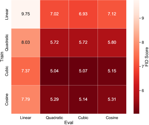
Figure 8: Comparison of FID on CIFAR10 with four schedulers: Linear, Quadratic, Cubic, Cosine, for both train and evaluation. Corrector sampling is not used in this experiment (, $\alpha_{t}=0$ in (26)), and temperature is set to 1.

Comparison with baselines.

In the following, we provide implementation details for producing Figure 3, that compares our schedulers and sampling algorithm with those employed by previous works.

Cubic Scheduler (Ours).

For the Cubic scheduler we set the corrector scheduler as above to,

$$\alpha_{t}=1+\alpha t^{a}(1-t)^{b},\quad\beta_{t}=\alpha_{t}-1,$$ (75)

and we search over the parameters $a,b\in\set{0,0.25,0.5,1,2,2.5,3}$, and $\alpha\in\set{6,8,10,12,14}$. Additionally, we search over the temperature $\in\set{1,0.9,0.8}$. We find that $a=2$, $b=0.25$, $\alpha=12$ give best FID.

Linear Scheduler (Campbell et al., 2024).

For the linear scheduler we search over two additional hyper-parameters of the method: (i) For corrector scheduler as in (26), we set $\alpha_{t}=1+t\eta$, $\beta_{t}=\alpha_{t}-1$, where $\eta$ is the stochasticity parameter as in Campbell et al. (2024), and search over $\eta\in\set{0,1,2,5,10,15}$. (ii) We search over temperature in $\set{1,0.9,0.8}$. Finally, we find that the best FID is a achieved by $\eta=10$ and temperature $0.9$.

MaskGIT (Chang et al., 2022).

For the MaskGIT we train and sample with the Cosine scheduler $\kappa(t)=1-\cos\parr{\frac{\pi}{2}t}$ which is reported to achieve best results by Chang et al. (2022). For sampling we adjust the code from the re-implementation of Besnier and Chen (2023). In addition, we also search over the temperature in $\set{1,0.9,0.8,0.7,0.6,0.5}$, and we find the best FID is achieved by temperature 1.

13 Code generation - qualitative examples

13.1 Success cases

⬇

from typing import List

\par\pardef below_zero(operations: List[int]) -> bool:

""" You’re given a list of deposit and withdrawal operations

on a bank account that starts with

zero balance. Your task is to detect if at any point the balance

of account fallls below zero, and

at that point function should return True.

Otherwise it should return False.

>>> below_zero([1, 2, 3])

False

>>> below_zero([1, 2, -4, 5])

True

"""

⬇

balance = 0

for operation in operations:

if balance + operation < 0:

return True

balance = balance + operation

return False

⬇

def encode_shift(s: str):

"""

returns encoded string by shifting every character by 5 in the alphabet.

"""

return "".join([chr(((ord(ch) + 5 - ord("a")) \par\pardef decode_shift(s: str):

"""

takes as input string encoded with encode_shift function.

Returns decoded string.

"""

⬇

decoded = []

for ch in s:

decoded.append(chr(((ord(ch) - 5 - ord("a")) return "".join(decoded)

⬇

from typing import List, Any

\par\pardef filter_integers(values: List[Any]) -> List[int]:

""" Filter given list of any python values only for integers

>>> filter_integers([’a’, 3.14, 5])

[5]

>>> filter_integers([1, 2, 3, ’abc’, {}, []])

[1, 2, 3]

"""

⬇

return [value for value in values if isinstance(value, int)]

⬇

def common(l1: list, l2: list):

"""Return sorted unique common elements for two lists.

>>> common([1, 4, 3, 34, 653, 2, 5], [5, 7, 1, 5, 9, 653, 121])

[1, 5, 653]

>>> common([5, 3, 2, 8], [3, 2])

[2, 3]

\par"""

⬇

return sorted(set(l1) & set(l2))

⬇

def fibfib(n: int):

"""The FibFib number sequence is a sequence similar to

the Fibbonacci sequnece that’s defined as follows:

fibfib(0) == 0

fibfib(1) == 0

fibfib(2) == 1

fibfib(n) == fibfib(n-1) + fibfib(n-2) + fibfib(n-3).

Please write a function to efficiently compute the

n-th element of the fibfib number sequence.

>>> fibfib(1)

0

>>> fibfib(5)

4

>>> fibfib(8)

24

"""

⬇

if n == 0:

return 0

elif n == 1:

return 0

elif n == 2:

return 1

else:

return fibfib(n-1) + fibfib(n-2) + fibfib(n-3)

13.2 Failure cases

⬇

def solve(s):

"""You are given a string s.

if s[i] is a letter, reverse its case from lower to upper or vise versa,

otherwise keep it as it is.

If the string contains no letters, reverse the string.

The function should return the resulted string.

Examples

solve("1234") = "4321"

solve("ab") = "AB"

solve("#a@C") = "#A@c"

"""

⬇

if s is None:

return ""

if len(s) == 0:

return s

# result string

res = str()

# to lower case

s = s.lower()

for i in range(len(s)):

ch = s[i]

if ch.islower():

res.append(ch)

elif ch.isupper():

res.append(ch.lower())

else:

res.append(ch)

return res

⬇

from typing import List, Tuple

\pardef rolling_max(numbers: List[int]) -> List[int]:

""" From a given list of integers, generate a list of rolling maximum element

found until given moment in the sequence.

>>> rolling_max([1, 2, 3, 2, 3, 4, 2])

[1, 2, 3, 3, 3, 4, 4]

"""

⬇

max_number = 0

result = []

for number in numbers:

max_number = max(result)

if number > max_number:

result.append(number)

else:

result = [max_number]

return result

⬇

def truncate_number(number: float) -> float:

""" Given a positive floating point number, it can be decomposed into

and integer part (largest integer smaller than given number) and decimals

(leftover part always smaller than 1).

\parReturn the decimal part of the number.

>>> truncate_number(3.5)

0.5

"""

⬇

return math.floor(number)

⬇

from typing import List, Tuple

\pardef sum_product(numbers: List[int]) -> Tuple[int, int]:

""" For a given list of integers, return a tuple consisting of a sum and a

product of all the integers in a list. Empty sum should be equal to 0 and

empty product should be equal to 1.

>>> sum_product([])

(0, 1)

>>> sum_product([1, 2, 3, 4])

(10, 24)

"""

⬇

if len(numbers) == 0 or numbers[0] == 0:

return 0, 1

sum = 0

product = 1

for num in numbers:

if abs(num) != 0:

product = product * num

sum += num

return sum, product

⬇

from typing import List

\pardef factorize(n: int) -> List[int]:

""" Return list of prime factors of given integer in the order from smallest

to largest. Each of the factors should be listed number of times corresponding

to how many times it appeares in factorization. Input number should be equal

to the product of all factors.

>>> factorize(8)

[2, 2, 2]

>>> factorize(25)

[5, 5]

>>> factorize(70)

[2, 5, 7]

"""

⬇

factors = []

factor = 1

for i in range(2, n):

factor *= i

while n factors.append(factor)

factor += 1

return factors

⬇

from typing import List, Optional

\pardef longest(strings: List[str]) -> Optional[str]:

""" Out of list of strings, return the longest one. Return the first one in

case of multiple strings of the same length. Return None in case the input

list is empty.

>>> longest([])

\par>>> longest([’a’, ’b’, ’c’])

’a’

>>> longest([’a’, ’bb’, ’ccc’])

’ccc’

"""

⬇

long = ""

for string in strings:

if len(string) > len(long):

long = string

return long

13.3 Infilling

⬇

def bubbleSort(arr):

n = len(arr)

# optimize code, so if the array is already sorted, it doesn’t need

# to go through the entire process

# Traverse through all array elements

for i in range(n-1):

\par# range(n) also work but outer loop will

# repeat one time more than needed.

# Last i elements are already in place

⬇

swapped = False

for j in range(0, n-i-1):

⬇

# traverse the array from 0 to n-i-1

# Swap if the element found is greater

# than the next element

if arr[j] > arr[j + 1]:

swapped = True

⬇

arr[j], arr[j + 1] = arr[j + 1], arr[j]

⬇

if not swapped:

# if we haven’t needed to make a single swap, we

# can just exit the main loop.

return

⬇

# Function to perform Breadth First Search on a graph

# represented using adjacency list

def bfs(adjList, |\colorbox{pastelyellow}{\strut{}source}|, visited):

# Create a queue for BFS

q = deque()

\par# Mark the current node as visited and enqueue it

visited[|\colorbox{pastelyellow}{\strut{}source}|] = True

q.append(|\colorbox{pastelyellow}{\strut{}source}|)

\par# Iterate over the queue

while q:

# Dequeue a vertex from queue and print it

currentNode = q.popleft()

print(|\colorbox{pastelyellow}{\strut{}currentNode}|, end=" ")

\par# Get all adjacent vertices of the dequeued vertex

# If an adjacent has not been visited, then mark it visited and enqueue it

for |\colorbox{pastelyellow}{\strut{}adjacent}| in adjList[|\colorbox{pastelyellow}{\strut{}currentNode}|]:

if not visited[|\colorbox{pastelyellow}{\strut{}adjacent}|]:

visited[|\colorbox{pastelyellow}{\strut{}adjacent}|] = True

q.append(|\colorbox{pastelyellow}{\strut{}adjacent}|)

⬇

# Returns index of x in arr if present, else -1

def binary_search(arr, |\colorbox{pastelyellow}{\strut{}low}|, |\colorbox{pastelyellow}{\strut{}high}|, x):

\par# Check base case

if |\colorbox{pastelyellow}{\strut{}high}| >= |\colorbox{pastelyellow}{\strut{}low}|:

\par|\colorbox{pastelyellow}{\strut{}mid}| = (|\colorbox{pastelyellow}{\strut{}high}| + |\colorbox{pastelyellow}{\strut{}low}|) // 2

\par# If element is present at the middle itself

if arr[|\colorbox{pastelyellow}{\strut{}mid}|] == x:

return mid

\par# If element is smaller than mid, then it can only

# be present in left subarray

elif arr[|\colorbox{pastelyellow}{\strut{}mid}|] > x:

return binary_search(arr, |\colorbox{pastelyellow}{\strut{}low}|, |\colorbox{pastelyellow}{\strut{}mid}| - 1, x)

\par# Else the element can only be present in right subarray

else:

return binary_search(arr, |\colorbox{pastelyellow}{\strut{}mid}| + 1, |\colorbox{pastelyellow}{\strut{}high}|, x)

\parelse:

# Element is not present in the array

return -1

⬇

# Python program for Dijkstra’s single

# source shortest path algorithm. The program is

# for adjacency matrix representation of the graph

class Graph():

\pardef __init__(self, vertices):

self.V = vertices

self.graph = [[0 for column in range(vertices)]

for row in range(vertices)]

\pardef printSolution(self, dist):

print("Vertex Distance from Source")

for node in range(self.V):

print(node, " ", dist[node])

\par# A utility function to find the vertex with

# minimum distance value, from the set of vertices

# not yet included in shortest path tree

def minDistance(self, dist, sptSet):

\par# Initialize minimum distance for next node

min = 1e7

\par# Search not nearest vertex not in the

# shortest path tree

for v in range(self.V):

if dist[v] < min and sptSet[v] == False:

min = dist[v]

min_index = v

\parreturn min_index

\par# Function that implements Dijkstra’s single source

# shortest path algorithm for a graph represented

# using adjacency matrix representation

def dijkstra(self, |\colorbox{pastelyellow}{\strut{}src}|):

\par|\colorbox{pastelyellow}{\strut{}dist}| = [1e7] * self.V

|\colorbox{pastelyellow}{\strut{}dist}|[src] = 0

|\colorbox{pastelyellow}{\strut{}processed}| = [False] * self.V

\parfor cout in range(self.V):

\par# Pick the minimum distance vertex from

# the set of vertices not yet processed.

# u is always equal to src in first iteration

|\colorbox{pastelyellow}{\strut{}uv}| = self.minDistance(dist, |\colorbox{pastelyellow}{processed}|)

\par# Put the minimum distance vertex in the

# shortest path tree

|\colorbox{pastelyellow}{processed}|[|\colorbox{pastelyellow}{uv}|] = True

\par# Update distance value of the adjacent vertices

# of the picked vertex only if the current

# distance is greater than new distance and

# the vertex in not in the shortest path tree

for |\colorbox{pastelyellow}{v}| in range(self.V):

if (self.graph[|\colorbox{pastelyellow}{uv}|][|\colorbox{pastelyellow}{v}|] > 0 and

|\colorbox{pastelyellow}{processed}|[|\colorbox{pastelyellow}{uv}|] == False and

|\colorbox{pastelyellow}{dist}|[|\colorbox{pastelyellow}{uv}|] > |\colorbox{pastelyellow}{dist}|[|\colorbox{pastelyellow}{cout}|] + self.graph[|\colorbox{pastelyellow}{uv}|][|\colorbox{pastelyellow}{v}|]):

|\colorbox{pastelyellow}{dist}|[|\colorbox{pastelyellow}{uv}|] = |\colorbox{pastelyellow}{dist}|[|\colorbox{pastelyellow}{cout}|] + self.graph[|\colorbox{pastelyellow}{uv}|][|\colorbox{pastelyellow}{v}|]

\parself.printSolution(dist)

14 Textual generations

We present below example generations for the proposed method together with several baseline methods. We provide both conditional and unconditional generations. For the conditional generations, we mark the prompt in gray.

14.1 Conditional generation.

The United States on Wednesday asked the UN Security Council to slap an oil embargo on North Korea and freeze the assets of leader Kim Jong-un, in response to Pyongyang’s response to the revelations it had restarted its nuclear work in March. “We will continue working to use maximum international pressure on North Korea to agree to the suspension of its nuclear program and reinstate sanctions,” said John Bolton, who served as National Security Advisor and Secretary of State under US President Bill Clinton. “Here is North Korea’s response to our sanctions,” Bolton wrote in a letter to House Minority Leader Nancy Pelosi. “We want you to know that the international community is seriously monitoring North Korea at this time. North Korea is still complying with our requests from the past few days,” Bolton said on Monday. “We have been working through the United Nations to provide the information that they gave us.” Asked to whether any international pressure will be put in place for North Korea to give up its nuclear weapons, Bolton said the United States can use maximum pressure to get North Korea to abandon its nuclear weapons if it wants. “We’ve been working to use maximum pressure on North Korea, through the Security Council, and we will continue to do so,” said White House Deputy Press Secretary Sarah Huckabee Sanders in Washington. “We’re committed to taking any steps necessary to help North Korea pursue its only option for peace, including in this period,” she added. The United States did not plan to produce any more oil at this time last year and had not planned to do so this year. “We believe that the North Korea approach is misguided in moving forward with its nuclear program to endanger peace and security in its homeland and neighbors in Asia,” said Bolton, adding that the US supplies its nuclear weapons. “We don’t want them to sell their nuclear weapons to other nations,” he said. Bolton said the US would look for pressure on North Korea, which has been known to use nuclear weapons, as leverage to negotiations with the US. “I will reiterate what I have said before. So, the US has to put pressure on North Korea. But who else is going to hold the cards? Somebody else has to hold the cards,” Mr Bolton said. Bolton described what the United States is prepared to do to get North Korea to agree to give up its weapons and asks for sanctions. “As far as I know, we have to use the pressure the reason for putting sanctions on North Korea,” he said, adding that the US does not plan to ask the UN Security Council for sanctions alone.

The defender is available for the Maribor first leg but his club believed he should be suspended. SNS Group Celtic made an administrative blunder which saw Efe Ambrose left behind in the midfield in the Maribor department and has given him a potential three-match ban today. Although Efe Ambrose will be suspended next Friday, according to reports in Scottish media, the Celtic defender will still be fit for the Champions League first leg at Celtic Stadium in the middle of August. However, the Celtic club wrongly thought that Efe should only receive a three-match ban because he is available for the first leg. Although Efe Ambrose may receive a three-match ban next Friday, Efe Ambrose was part of the Celtic squad for the last match against Liverpool. However, says SNS Group Celtic he was making a tactical error and was left behind in midfield. It is understood that Efe Ambrose did not make the final squad and only played 11 games for the club this season. Efe Ambrose made his professional debut for Celtic in 2008 but spent nine months looking for a new club to return to. With a career-high 72 Celtic appearances, Efe is among Celtic’s most capped players ever.

Carl Jara aka Grain Damaged is an award-winning, professional sand sculptor from Cleveland, Ohio. Jara says he has known since high-school that he wanted to be an artist. After studying English and Art History at the Northeastern University, Jara says one semester he started carving a custom sculpture into sand molds, but didn’t know how to do it. With the help of an instructor, he found out and learned how to use rubber molds to make art. Later, he made the decision to learn how to use sand and sculpt himself. In addition to how he makes his own sculptures, Jara says he does special events for comics companies such as Stan Lee and also for institutions like local community colleges and universities. In November of this year, he won the WWHS, The Very Art Of The Very Things Cleveland competition. Afterward, he will continue carving for clients in the comics industry and looks forward to sand sculpting in Cleveland. The Artist is professional sculptor who has been making art, for over 25 years, in various shapes and sizes.The artist says art is all about relationships and the best way to go into the heart is to create art. The artist has taught in various high schools in the Cleveland area and has taught a full time Honors Studio for High School students in grades 6, 7, and 8 time for over 20 years. Since Art is a personal form of artistic expression, he works individually in a way that allows the student that his work engages their imagination and presents ideas in ways that inform and challenge their own paths. Miguel Romano is a professional artist who worked in 3D modeling and animation in the areas of web design and production. The artist currently works as a digital artist in the ad and mass communication industries. In coming to Concrete Cleveland, he is excited to apply the 3D development and production skills he have to his work. The artist has a BFA in sculpture from Ohio University, along with an MFA in sculpture. We look forward to seeing his work very soon! Designed and installed by Concrete This Week. He is a guy originally from Cleveland, Ohio where he pursued a career as a nurse. He then moved to the Atlanta, GA area where he returned to school with a BSN and a BS in nursing and is a licensed nurse. He is a proud sorority brother and still has extra-curricular, as well as taking music lessons and the occasional play. He is a lovely asset at Concrete Cleveland and looks forward to seeing concrete

References

- Ahn et al. (2024) Janice Ahn, Rishu Verma, Renze Lou, Di Liu, Rui Zhang, and Wenpeng Yin. Large language models for mathematical reasoning: Progresses and challenges. arXiv preprint arXiv:2402.00157, 2024.
- Albergo and Vanden-Eijnden (2022) Michael S Albergo and Eric Vanden-Eijnden. Building normalizing flows with stochastic interpolants. arXiv preprint arXiv:2209.15571, 2022.
- Austin et al. (2021a) Jacob Austin, Daniel D Johnson, Jonathan Ho, Daniel Tarlow, and Rianne Van Den Berg. Structured denoising diffusion models in discrete state-spaces. Advances in Neural Information Processing Systems, 34:17981–17993, 2021a.
- Austin et al. (2021b) Jacob Austin, Augustus Odena, Maxwell Nye, Maarten Bosma, Henryk Michalewski, David Dohan, Ellen Jiang, Carrie Cai, Michael Terry, Quoc Le, et al. Program synthesis with large language models. arXiv preprint arXiv:2108.07732, 2021b.
- Besnier and Chen (2023) Victor Besnier and Mickael Chen. A pytorch reproduction of masked generative image transformer, 2023.
- Blattmann et al. (2023) Andreas Blattmann, Tim Dockhorn, Sumith Kulal, Daniel Mendelevitch, Maciej Kilian, Dominik Lorenz, Yam Levi, Zion English, Vikram Voleti, Adam Letts, et al. Stable video diffusion: Scaling latent video diffusion models to large datasets. arXiv preprint arXiv:2311.15127, 2023.
- Brown et al. (2020) Tom Brown, Benjamin Mann, Nick Ryder, Melanie Subbiah, Jared D Kaplan, Prafulla Dhariwal, Arvind Neelakantan, Pranav Shyam, Girish Sastry, Amanda Askell, et al. Language models are few-shot learners. Advances in neural information processing systems, 33:1877–1901, 2020.
- Campbell et al. (2022) Andrew Campbell, Joe Benton, Valentin De Bortoli, Thomas Rainforth, George Deligiannidis, and Arnaud Doucet. A continuous time framework for discrete denoising models. Advances in Neural Information Processing Systems, 35:28266–28279, 2022.
- Campbell et al. (2024) Andrew Campbell, Jason Yim, Regina Barzilay, Tom Rainforth, and Tommi Jaakkola. Generative flows on discrete state-spaces: Enabling multimodal flows with applications to protein co-design. arXiv preprint arXiv:2402.04997, 2024.
- Chang et al. (2022) Huiwen Chang, Han Zhang, Lu Jiang, Ce Liu, and William T Freeman. Maskgit: Masked generative image transformer. In Proceedings of the IEEE/CVF Conference on Computer Vision and Pattern Recognition, pages 11315–11325, 2022.
- Chang et al. (2023) Huiwen Chang, Han Zhang, Jarred Barber, AJ Maschinot, Jose Lezama, Lu Jiang, Ming-Hsuan Yang, Kevin Murphy, William T Freeman, Michael Rubinstein, et al. Muse: Text-to-image generation via masked generative transformers. arXiv preprint arXiv:2301.00704, 2023.
- Chen et al. (2021) Mark Chen, Jerry Tworek, Heewoo Jun, Qiming Yuan, Henrique Ponde de Oliveira Pinto, Jared Kaplan, Harri Edwards, Yuri Burda, Nicholas Joseph, Greg Brockman, et al. Evaluating large language models trained on code. arXiv preprint arXiv:2107.03374, 2021.
- Chen et al. (2022) Ting Chen, Ruixiang Zhang, and Geoffrey E. Hinton. Analog bits: Generating discrete data using diffusion models with self-conditioning. ArXiv, 2022.
- Copet et al. (2024) Jade Copet, Felix Kreuk, Itai Gat, Tal Remez, David Kant, Gabriel Synnaeve, Yossi Adi, and Alexandre Défossez. Simple and controllable music generation. Advances in Neural Information Processing Systems, 36, 2024.
- Dhariwal and Nichol (2021) Prafulla Dhariwal and Alexander Nichol. Diffusion models beat gans on image synthesis. Advances in neural information processing systems, 34:8780–8794, 2021.
- Dieleman et al. (2022) Sander Dieleman, Laurent Sartran, Arman Roshannai, Nikolay Savinov, Yaroslav Ganin, Pierre H Richemond, Arnaud Doucet, Robin Strudel, Chris Dyer, Conor Durkan, et al. Continuous diffusion for categorical data. arXiv preprint arXiv:2211.15089, 2022.
- Esser et al. (2024) Patrick Esser, Sumith Kulal, Andreas Blattmann, Rahim Entezari, Jonas Müller, Harry Saini, Yam Levi, Dominik Lorenz, Axel Sauer, Frederic Boesel, et al. Scaling rectified flow transformers for high-resolution image synthesis. arXiv preprint arXiv:2403.03206, 2024.
- Ferruz and Höcker (2022) Noelia Ferruz and Birte Höcker. Controllable protein design with language models. Nature Machine Intelligence, 4(6):521–532, 2022.
- Ghazvininejad et al. (2019) Marjan Ghazvininejad, Omer Levy, Yinhan Liu, and Luke Zettlemoyer. Mask-predict: Parallel decoding of conditional masked language models. arXiv preprint arXiv:1904.09324, 2019.
- Gokaslan and Cohen (2019) Aaron Gokaslan and Vanya Cohen. Openwebtext corpus. http://Skylion007.github.io/OpenWebTextCorpus, 2019.
- Han et al. (2022) Xiaochuang Han, Sachin Kumar, and Yulia Tsvetkov. Ssd-lm: Semi-autoregressive simplex-based diffusion language model for text generation and modular control. arXiv preprint arXiv:2210.17432, 2022.
- Hassid et al. (2024) Michael Hassid, Tal Remez, Tu Anh Nguyen, Itai Gat, Alexis Conneau, Felix Kreuk, Jade Copet, Alexandre Defossez, Gabriel Synnaeve, Emmanuel Dupoux, et al. Textually pretrained speech language models. Advances in Neural Information Processing Systems, 36, 2024.
- He et al. (2022) Zhengfu He, Tianxiang Sun, Kuan Wang, Xuanjing Huang, and Xipeng Qiu. Diffusionbert: Improving generative masked language models with diffusion models. In Annual Meeting of the Association for Computational Linguistics, 2022.
- Heusel et al. (2017) Martin Heusel, Hubert Ramsauer, Thomas Unterthiner, Bernhard Nessler, and Sepp Hochreiter. Gans trained by a two time-scale update rule converge to a local nash equilibrium. In Advances in Neural Information Processing Systems (NeurIPS), 2017.
- Ho et al. (2020) Jonathan Ho, Ajay Jain, and Pieter Abbeel. Denoising diffusion probabilistic models. Advances in neural information processing systems, 33:6840–6851, 2020.
- Hoogeboom et al. (2021) Emiel Hoogeboom, Didrik Nielsen, Priyank Jaini, Patrick Forré, and Max Welling. Argmax flows and multinomial diffusion: Learning categorical distributions. Advances in Neural Information Processing Systems, 34:12454–12465, 2021.
- Imani et al. (2023) Shima Imani, Liang Du, and Harsh Shrivastava. Mathprompter: Mathematical reasoning using large language models. In Proceedings of the 61st Annual Meeting of the Association for Computational Linguistics (Volume 5: Industry Track), pages 37–42, 2023.
- Kreuk et al. (2022) Felix Kreuk, Gabriel Synnaeve, Adam Polyak, Uriel Singer, Alexandre Défossez, Jade Copet, Devi Parikh, Yaniv Taigman, and Yossi Adi. Audiogen: Textually guided audio generation. arXiv preprint arXiv:2209.15352, 2022.
- Krizhevsky et al. (2009) Alex Krizhevsky, Geoffrey Hinton, et al. Learning multiple layers of features from tiny images. arXiv, 2009.
- Li et al. (2023) Raymond Li, Loubna Ben Allal, Yangtian Zi, Niklas Muennighoff, Denis Kocetkov, Chenghao Mou, Marc Marone, Christopher Akiki, Jia Li, Jenny Chim, et al. Starcoder: may the source be with you! arXiv preprint arXiv:2305.06161, 2023.
- Li et al. (2022) Xiang Lisa Li, John Thickstun, Ishaan Gulrajani, Percy Liang, and Tatsunori Hashimoto. Diffusion-lm improves controllable text generation. ArXiv, 2022.
- Lin et al. (2022) Zheng-Wen Lin, Yeyun Gong, Yelong Shen, Tong Wu, Zhihao Fan, Chen Lin, Weizhu Chen, and Nan Duan. Genie : Large scale pre-training for generation with diffusion model. In ArXiv, 2022.
- Lipman et al. (2022) Yaron Lipman, Ricky TQ Chen, Heli Ben-Hamu, Maximilian Nickel, and Matt Le. Flow matching for generative modeling. arXiv preprint arXiv:2210.02747, 2022.
- Liu et al. (2022) Xingchao Liu, Chengyue Gong, and Qiang Liu. Flow straight and fast: Learning to generate and transfer data with rectified flow. arXiv preprint arXiv:2209.03003, 2022.
- Lou et al. (2023) Aaron Lou, Chenlin Meng, and Stefano Ermon. Discrete diffusion language modeling by estimating the ratios of the data distribution. arXiv preprint arXiv:2310.16834, 2023.
- Lovelace et al. (2022) Justin Lovelace, Varsha Kishore, Chao gang Wan, Eliot Shekhtman, and Kilian Q. Weinberger. Latent diffusion for language generation. ArXiv, 2022.
- Madani et al. (2023) Ali Madani, Ben Krause, Eric R Greene, Subu Subramanian, Benjamin P Mohr, James M Holton, Jose Luis Olmos, Caiming Xiong, Zachary Z Sun, Richard Socher, et al. Large language models generate functional protein sequences across diverse families. Nature Biotechnology, 41(8):1099–1106, 2023.
- Norris (1998) James R Norris. Markov chains. Number 2. Cambridge university press, 1998.
- Peebles and Xie (2022) William Peebles and Saining Xie. Scalable diffusion models with transformers. arXiv preprint arXiv:2212.09748, 2022.
- Pooladian et al. (2023) Aram-Alexandre Pooladian, Heli Ben-Hamu, Carles Domingo-Enrich, Brandon Amos, Yaron Lipman, and Ricky TQ Chen. Multisample flow matching: Straightening flows with minibatch couplings. arXiv preprint arXiv:2304.14772, 2023.
- Radford et al. (2019) Alec Radford, Jeff Wu, Rewon Child, David Luan, Dario Amodei, and Ilya Sutskever. Language models are unsupervised multitask learners. 2019. https://api.semanticscholar.org/CorpusID:160025533.
- Rombach et al. (2022) Robin Rombach, Andreas Blattmann, Dominik Lorenz, Patrick Esser, and Björn Ommer. High-resolution image synthesis with latent diffusion models. In Proceedings of the IEEE/CVF conference on computer vision and pattern recognition, pages 10684–10695, 2022.
- Romera-Paredes et al. (2024) Bernardino Romera-Paredes, Mohammadamin Barekatain, Alexander Novikov, Matej Balog, M Pawan Kumar, Emilien Dupont, Francisco JR Ruiz, Jordan S Ellenberg, Pengming Wang, Omar Fawzi, et al. Mathematical discoveries from program search with large language models. Nature, 625(7995):468–475, 2024.
- Roziere et al. (2023) Baptiste Roziere, Jonas Gehring, Fabian Gloeckle, Sten Sootla, Itai Gat, Xiaoqing Ellen Tan, Yossi Adi, Jingyu Liu, Tal Remez, Jérémy Rapin, et al. Code llama: Open foundation models for code. arXiv preprint arXiv:2308.12950, 2023.
- Savinov et al. (2021) Nikolay Savinov, Junyoung Chung, Mikolaj Binkowski, Erich Elsen, and Aaron van den Oord. Step-unrolled denoising autoencoders for text generation. arXiv preprint arXiv:2112.06749, 2021.
- Singer et al. (2022) Uriel Singer, Adam Polyak, Thomas Hayes, Xi Yin, Jie An, Songyang Zhang, Qiyuan Hu, Harry Yang, Oron Ashual, Oran Gafni, et al. Make-a-video: Text-to-video generation without text-video data. arXiv preprint arXiv:2209.14792, 2022.
- Song and Ermon (2019) Yang Song and Stefano Ermon. Generative modeling by estimating gradients of the data distribution. Advances in neural information processing systems, 32, 2019.
- Song et al. (2020) Yang Song, Jascha Sohl-Dickstein, Diederik P Kingma, Abhishek Kumar, Stefano Ermon, and Ben Poole. Score-based generative modeling through stochastic differential equations. arXiv preprint arXiv:2011.13456, 2020.
- Stark et al. (2024) Hannes Stark, Bowen Jing, Chenyu Wang, Gabriele Corso, Bonnie Berger, Regina Barzilay, and Tommi Jaakkola. Dirichlet flow matching with applications to dna sequence design. arXiv preprint arXiv:2402.05841, 2024.
- Su et al. (2024) Jianlin Su, Murtadha Ahmed, Yu Lu, Shengfeng Pan, Wen Bo, and Yunfeng Liu. Roformer: Enhanced transformer with rotary position embedding. Neurocomputing, 568:127063, 2024.
- Tong et al. (2023) Alexander Tong, Nikolay Malkin, Guillaume Huguet, Yanlei Zhang, Jarrid Rector-Brooks, Kilian Fatras, Guy Wolf, and Yoshua Bengio. Improving and generalizing flow-based generative models with minibatch optimal transport. arXiv preprint arXiv:2302.00482, 2023.
- Touvron et al. (2023) Hugo Touvron, Louis Martin, Kevin Stone, Peter Albert, Amjad Almahairi, Yasmine Babaei, Nikolay Bashlykov, Soumya Batra, Prajjwal Bhargava, Shruti Bhosale, et al. Llama 2: Open foundation and fine-tuned chat models. arXiv preprint arXiv:2307.09288, 2023.
- Zhang et al. (2024) Qiang Zhang, Keyang Ding, Tianwen Lyv, Xinda Wang, Qingyu Yin, Yiwen Zhang, Jing Yu, Yuhao Wang, Xiaotong Li, Zhuoyi Xiang, et al. Scientific large language models: A survey on biological & chemical domains. arXiv preprint arXiv:2401.14656, 2024.
- Zhao et al. (2023) Wayne Xin Zhao, Kun Zhou, Junyi Li, Tianyi Tang, Xiaolei Wang, Yupeng Hou, Yingqian Min, Beichen Zhang, Junjie Zhang, Zican Dong, et al. A survey of large language models. arXiv preprint arXiv:2303.18223, 2023.
- Ziv et al. (2024) Alon Ziv, Itai Gat, Gael Le Lan, Tal Remez, Felix Kreuk, Alexandre Défossez, Jade Copet, Gabriel Synnaeve, and Yossi Adi. Masked audio generation using a single non-autoregressive transformer. arXiv preprint arXiv:2401.04577, 2024.