Exploring the Effectiveness of Object-Centric Representations in Visual Question Answering: Comparative Insights with Foundation Models

Abstract

Object-centric (OC) representations, which represent the state of a visual scene by modeling it as a composition of objects, have the potential to be used in various downstream tasks to achieve systematic compositional generalization and facilitate reasoning. However, these claims have not been thoroughly analyzed yet. Recently, foundation models have demonstrated unparalleled capabilities across diverse domains from language to computer vision, marking them as a potential cornerstone of future research for a multitude of computational tasks. In this paper, we conduct an extensive empirical study on representation learning for downstream Visual Question Answering (VQA), which requires an accurate compositional understanding of the scene. We thoroughly investigate the benefits and trade-offs of OC models and alternative approaches including large pre-trained foundation models on both synthetic and real-world data, and demonstrate a viable way to achieve the best of both worlds. The extensiveness of our study, encompassing over 800 downstream VQA models and 15 different types of upstream representations, also provides several additional insights that we believe will be of interest to the community at large.

1 Introduction

Object-centric (OC) learning aims to represent the physical world’s inherent structure, assuming visual scenes consist of entities or objects and employing this as an inductive bias for neural networks [1, 2, 3, 4, 5, 6, 7, 8, 9, 10]. Applied in various domains like visual reasoning [11, 12, 13, 14, 15, 16, 17] and image and video generation [18, 5, 6, 19, 20], these representations play a crucial role in capturing compositional and causal structures, with the potential to improve the generalizability and interpretability of AI algorithms [21, 22, 23, 24, 25]. Breaking down scenes into conceptual elements corresponding to causal factors aligns with the idea that causal models play a crucial role in achieving human-level generalization [26, 27, 28, 29].

While OC representations thus provide a way of representing the state of a visual scene, a comprehensive understanding of these representations is still an ongoing exploration. Recently, there have been several works on evaluating OC representations. Some studies evaluate object-centric models in terms of reconstruction and segmentation accuracy, and quantify the quality and information content of object representations via a downstream object property prediction task [30, 31]. Arguing that a major goal of representation learning is to facilitate downstream tasks, Yoon et al. [32] focuses on the evaluation of the representations in reinforcement learning, which requires a thorough understanding of the environment in terms of objects and the relations between them. However, a more direct quantification of the role of object-centric representations for reasoning is still missing.

In the rapidly evolving landscape of deep learning, foundation models, often characterized by self-supervised and large-scale pre-training, have demonstrated unparalleled capabilities in generalization and zero-shot learning, showcasing their prowess in tasks across diverse domains from natural language processing to computer vision [33, 34, 35, 36, 37, 38, 39, 40, 41, 42]. Despite their widespread success, foundation models have not been comprehensively analyzed and compared with OC models.

Our main contributions are the following:

• We conduct a large empirical study on representation learning for downstream Visual Question Answering (VQA) [43, 44] on three synthetic and one real-world multi-object datasets. In our extensive evaluation, we train overall 852 downstream transformer models for VQA, involving 15 different types of upstream representation models, ranging from VAEs to state-of-the-art OC methods to large pre-trained foundation models.

• We identify and investigate the trade-offs between large foundation models and object-centric models. We observe that, without any fine-tuning or hyperparameter adjustment, foundation models perform comparably to the top-performing OC models. On the other hand, they typically require more compute and larger downstream models. We find that applying the OC inductive bias to foundation models effectively achieves the best of both worlds, reducing the downstream computational needs while achieving comparable or better performance and obtaining more explicit representations.

• We present several additional insights regarding, among other things, the correlation between performances on VQA and a simpler downstream task, the relationship between upstream and downstream performance of OC models, the effect of training set size on VQA performance, the difference between different question types, and a deeper analysis of the lobal (single-vector) representations of traditional VAEs.

2 Related Works

Object-Centric Learning.

Object-centric (OC) learning has gained attention over the past few years [45, 46, 47, 48, 49, 50, 51, 52, 53, 54, 55, 56, 2, 3, 4, 20, 18, 57, 58, 19, 10, 59, 60]. OC models aim to learn visual representations without supervision by treating each image as a composition of objects. Among them, Slot Attention [2] stands out as a popular model and a crucial component in several recent state-of-the-art models. Numerous enhancements have been proposed, including improvements of the Slot Attention module [61, 62, 63] or adding additional modules on top [64], using a transformer decoder instead of the original mixture-based decoder [49, 6], replacing the CNN backbone with a pre-trained model [7], and integrating diffusion models with Slot Attention [9, 8, 20].

Evaluation of Object-Centric Representations.

OC methods have been applied in several works in visual reasoning [11, 12, 13, 14, 15, 16, 17, 65] and some of these works try to address the Visual Question Answering task itself. Ding et al. [12] propose a new method to address the VQA in videos and run a transformer over slots obtained from a pre-trained MONet [4], and text tokens of the question, and applies an MLP on top to predict the answer. The method proposed by Wu et al. [13] reasons over the object representations of Slot Attention to model spatiotemporal relationships, and predicts future object states. Their framework is also applied to a VQA downstream task.

In addition, a few works focus more specifically on the evaluation of OC representations. Weis et al. [66] designs a benchmark over only OC video models and analyzes their performance over different tracking scenarios relevant to natural videos. Yang and Yang [67] evaluates OC representations and shows their shortcomings in segmenting objects in a real-world dataset. Dittadi et al. [30] evaluates the representations indirectly in the context of reconstruction loss, segmentation quality, and object property prediction, and analyzes their generalization and robustness. Papa et al. [31] uses the same evaluation metrics on a dataset with complex textures. Yoon et al. [32] evaluates the representations on more practically relevant downstream tasks in reinforcement learning and includes a wider range of methods compared to the previous works. Finally, Driess et al. [65] demonstrates the suitability of OC representations in planning and VQA tasks within a robotic environment. However, the assessment is done on a single OC baseline in the presence of a Large Language Model (LLM) and the VQA setup is restricted to particular scenarios. In our work, we are interested in investigating the suitability of different types of representation, including object-centric ones, for reasoning tasks. To this end, we opt to more directly assess the suitability of representations for reasoning through VQA.

3 Experimental Setup

In this section, we provide an overview of our experimental setup. First, we introduce the downstream task used in our experiments to evaluate representations. We then outline the upstream representation models, the datasets and metrics, and the concrete setup for learning the downstream task.

3.1 Visual Question Answering

In this paper, we evaluate the performance attainable on a Visual Question Answering (VQA) task [43] from different representations of the visual scenes. With questions that can involve any number of objects from just one to all the objects in an image, VQA presents a more demanding challenge compared to object-level tasks. It requires a thorough understanding of the image and complex reasoning about objects and their relationships. We therefore choose VQA as a benchmark to directly assess the suitability of different representations for reasoning.

Given an image, the task is to provide an accurate answer to a natural language question such as “How many tiny green objects are made of the same material as the purple cube?”. The questions are usually about how many objects there are, whether an object with a specific attribute (e.g., shape) exists, and what properties they have in relation to another set of objects in an image. The possible answers include “yes”, “no”, and various numerical and categorical values. Further details are provided in Section C.2.

Our framework, summarized in Fig. 1, consists of: (1) an upstream model that provides high-level representations of an image, (2) a fixed pre-trained text embedding model that converts a question in natural language to text embeddings, and (3) a downstream model that takes as input the image representation and the text embedding and outputs the answer to the question. We will elaborate on each part in the following sections.

3.2 Upstream Models

To investigate OC representations, we consider three types of representations: global, fixed-region, and object-centric. Global representations encode the image into a single vector which contains high-level information about the image. Fixed-region representations consist of a fixed number of vectors, each loosely corresponding to a specific region within the image. OC representations consist of a set of vectors, each ideally corresponding to a single object.

Table 1: Summary of models included in our study.

Model	Representation Type	Training Regime
DINOv2 [68]	Fixed-Region	Pre-training
MAE [69]	Fixed-Region	Pre-training
CLIP [70]	Fixed-Region	Pre-training
VQ-AE [42]	Fixed-Region	Pre-training
KL-AE [42]	Fixed-Region	Pre-training
ResNet50 [71]	Fixed-Region	Pre-training
CNN [72]	Fixed-Region	End-to-End Training
MultiCNN [57]	Object-Centric	End-to-End Training
Slot Attention [2]	Object-Centric	Dataset-Specific Pre-training
ResNet Slot Attention [61]	Object-Centric	Dataset-Specific Pre-training
MONet [4]	Object-Centric	Dataset-Specific Pre-training
SPACE [3]	Object-Centric	Dataset-Specific Pre-training
STEVE [6]	Object-Centric	Dataset-Specific Pre-training
DINOSAURv2 [7]	Object-Centric	Dataset-Specific Pre-training
VAE [73]	Global	Dataset-Specific Pre-training

The evaluated models are summarized in Table 1. As OC baselines, we use MONet [4], SPACE [3], and Slot Attention (SA) [2]. We also include ResNet SA [61], an improved version of the standard SA autoencoder with the following modifications: the backbone is replaced by a ResNet34 [71] without pre-training; a larger feature map resolution is used in both the encoder and the decoder; and the slot initializations are learnable. We also consider STEVE [6], a state-of-the-art OC video model for complex and naturalistic videos. STEVE is a more robust version of SLATE [5] combining the SLATE decoder with a standard slot-level recurrent model. To adapt STEVE to images, we simply consider images as 1-frame videos, following the authors’ recommendation. Furthermore, as the last OC baseline, we consider DINOSAUR [7], a state-of-the-art OC image model, and replace its pre-trained DINO [74] backbone with DINOv2 [68]—we refer to this model as DINOSAURv2. Following previous work, we also consider multiple CNNs [57, 75, 32], each CNN being expected to capture one object in the image, and train all of them end-to-end together with the downstream model—we refer to this approach as MultiCNN.

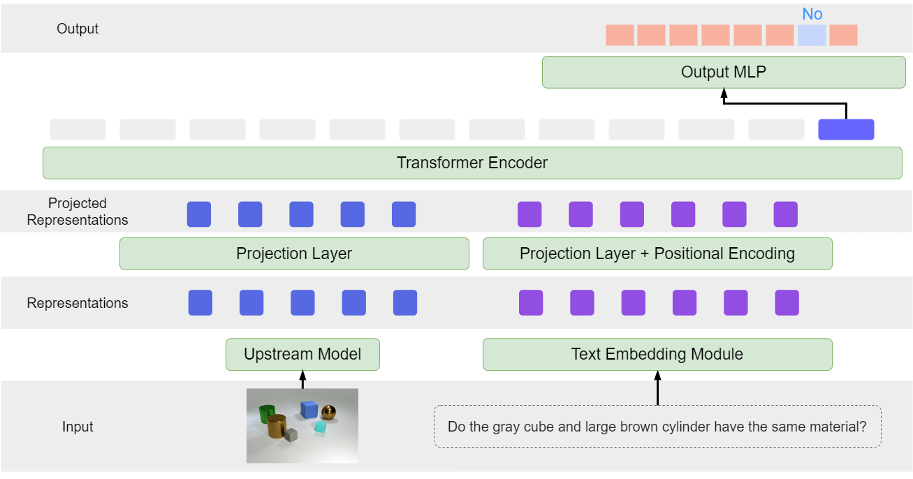
Figure 1: An overview of our framework. Starting from an image and a question, we first extract image and question representations, by applying the upstream model and the text embedding module, respectively. The obtained representations are then passed to the projection layer and then, a positional encoding is applied to the text representations. Next, both are concatenated and a transformer model is applied to the combined sequence. Finally, The answer to the question is obtained by an MLP that takes the transformed value of the CLS token and produces a probability vector over all possible answers.

As a classic benchmark for fixed-region representations [32, 7], we include a pre-trained ResNet50 [71]. We also utilize two pre-trained autoencoders from Latent Diffusion Models (LDM) [42], one with a KL regularization and the other one with a vector quantization layer, both with a scaling factor of $16$. We refer to them as KL-AE and VQ-AE, respectively. Additionally, we use pre-trained versions of DINOv2 [68, 76], Masked Autoencoder (MAE) [69], and CLIP [70], all of which have achieved outstanding performance as a backbone in a diverse array of tasks. Following previous works [15, 72, 32], we also implement a simple CNN, and train it end-to-end with the downstream model. As a baseline providing a global representation, we follow Dittadi et al. [30] and consider a variation of vanilla variational autoencoders (VAE) [77, 78] with a broadcast decoder [73]. Finally, for each dataset, we include a naive baseline that always predicts the majority class and achieves the highest possible accuracy without assuming any information about the data.

Regarding the training of upstream models, we have $3$ different types of models: pre-trained foundation models, pre-trained dataset-specific models, and end-to-end models. Pre-trained foundation models have been trained on large-scale datasets and tasks, serving as the basis for transfer learning in various applications. DINOv2, MAE, CLIP, VQ-AE, KL-AE, and ResNet50 belong to this category that we use off-the-shelf without fine-tuning, in all experiments. Dataset-specific pre-trained models are first trained with an autoencoding objective (only using images, disregarding the questions) on the same dataset that will be used for VQA with their original training procedures and hyperparameter choices. They are subsequently frozen, similarly to foundation models. MONet, SPACE, SA, ResNet SA, STEVE, DINOSAURv2, and VAE are in this category. Finally, end-to-end models are trained from scratch alongside the downstream model to solve the VQA task directly. CNN and MultiCNN belong to this category. For more information about the upstream models, see Section B.1.

3.3 Datasets

Synthetic.

We utilize three popular multi-object datasets in our experiments: Multi-dSprites [79], a variation of CLEVR [44] with $6$ objects known as CLEVR6 [80, 2, 30], and CLEVRTex [81] which is a variation of CLEVR featuring synthetic scenes with diverse shapes, textures and photo-mapped materials. This dataset is closer to real-world datasets in terms of visual complexity. To analyze the effect of training data size, we consider $4$ different training data sizes in Multi-dSprites with $40$k, $80$k, $160$k, and $320$k unique images, with the $320$k version as the default version. Each image in the multi-object datasets consists of a background with a fixed color and a set of objects with different properties. Originally, only CLEVR contains questions associated with each image. To make the other datasets applicable to the same VQA task, we augment them with several questions (roughly 40-50) for each image, by adapting the question generation mechanism of Johnson et al. [44] to each dataset. We use this to generate different types of questions, with possible answers including “yes”, “no”, natural numbers up to the maximum number of objects, and all possible values of object properties. For more details about the datasets and question generation, see Appendix C.

Real-World.

Additionally, we extend our results to real-world scenarios with the VQA-v2 [82, 43] dataset. VQA-v2 consists of open-ended questions about images sourced from MS COCO 2014 [83], a real-world multi-object dataset. Recently, COCO has been increasingly utilized in object-centric literature [7, 9, 8], marking a significant advancement in complexity compared to datasets typically used to evaluate object-centric models. VQA-v2 features a diverse range of questions and possible answers. To align with the same pipeline used for synthetic datasets, we limit the questions to yes/no and questions with numeric answers ranging from 0 to 14. This results in a total of 17 possible answers. For more details about the dataset and the preprocessing, see Appendix C.

3.4 Metrics

Following previous works [12, 13], we measure performance in our VQA downstream task by average accuracy. As metrics for the upstream OC models, we use the Mean Squared Error (MSE) of the reconstructions, and 3 segmentation metrics: the Adjusted Rand Index (ARI) [84], Segmentation Covering (SC) [85], and mean Segmentation Covering (mSC) [50]. All of these metrics have been extensively used in previous studies [2, 30, 6, 61]. See Appendix D for more details about the metrics.

3.5 Framework Setup

Our VQA framework, depicted in Fig. 1, closely follows Ding et al. [12]. Given a pair $(x,q)$ where $x\in\mathbb{R}^{3\times H\times W}$ denotes an image of height $H$ and width $W$, and $q$ denotes a question, the task is to select the correct answer from the set of all possible answers. Since the number of answers in each dataset is relatively small, it is not necessary to generate text tokens as the answers, and similarly to Ding et al. [12], we stick to the simpler case of predicting a probability vector over all possible answers in the dataset. Another key aspect to consider is that our primary focus is on evaluating representations while the method for generating questions and the format of the answers hold less significance in this context.

Image and Text Representations.

Given a data pair $(x,q)$, the upstream model computes the image representation $z$. In global representations, $z$ is a vector of size $D_{glob}$. In OC models, $z$ is a $N_{slots}\times D_{oc}$ matrix where $N_{slots}$ is the number of slots in the OC model. In fixed-region representations, $z$ is a feature map of size $P_{H}\times P_{W}\times D_{fr}$ where the first two dimensions correspond to the feature map sizes and the third dimension is the size of the representation. For more details about obtaining image representations from the upstream models, see Section B.1.

To embed the question $q$ from text format to word embeddings, we use the Text-to-Text Transfer Transformer [T5; 86] which outputs a matrix $t$ of size $N_{tokens}\times D_{emb}$ representing the embeddings of the tokens in the question where the dimensions correspond to the number of tokens and the embedding size, respectively. See Section B.2 for more details.

Unifying Image Representations.

In order to use different types of image representations in the downstream model which follows a transformer architecture and will be explained later on, it is necessary to unify the format of representations and convert them to a sequence. We use $z$ as it is for OC representations since each slot corresponds to an object, and can be separately used as an item in the sequence. We reshape fixed-region representations by flattening the spatial dimensions, obtaining a matrix of size $P_{H}P_{W}\times D_{fr}$.

For global representations, we split the single vector $z$ into $K$ vectors of size $D_{glob}/K$. Here, $K$ roughly corresponds to the number of slots in an OC model. In other words, we treat $z$ as a sequence of length $K$ with a latent size of $D_{glob}/K$. While we observed this to be the most effective option in terms of downstream performance, we also considered three alternative approaches. The first applies a 2-layer MLP to $z$ and subsequently splits the output similarly to what described above; the second method treats the single vector $z$ as one token in a sequence of length 1; the third splits $z$ into $D_{glob}$ sequences of size $1$. All these approaches showed poorer downstream performance, and in addition, the last one is computationally expensive due to a large sequence length.

Downstream Model.

Following previous works on VQA [12, 87, 88], we use a transformer-based architecture [89]. Having $t$ and the reformatted $z$ as text and image representations, we apply a separate linear layer on each to make the latent size and the embedding size equal, and we get $t^{\prime}$ and $z^{\prime}$, respectively. Then, to inform the downstream model about the order of words, we apply a sinusoidal positional encoding layer to $t^{\prime}$. Additionally, following Ding et al. [12], we augment each vector in $z^{\prime}$ and $t^{\prime}$ with a $2$-dimensional one-hot vector indicating whether the input is from the image representation or the text, and the latent size for both will become $D_{model}$. We introduce a trainable vector $\textit{CLS}\in\mathbb{R}^{D_{model}}$, akin to the CLS token in BERT [87], to generate classification results. In the final step, we concatenate $z^{\prime}$, $t^{\prime}$, and the CLS token and pass this sequence through a transformer with $N_{t}$ layers. An MLP classifier then takes the transformed CLS token and outputs a probability vector over all possible answers.

3.6 Limitations

While our goal is to execute a robust and informative experimental study to address the research questions identified in Section 1, it’s important to acknowledge inherent limitations related to datasets, models, and evaluations. First, despite the substantial variation in complexity and visual properties among the considered datasets, they mostly consist of synthetic images, with only one real-world dataset included. In these synthetic images, object properties remain independent of each other and are also independent between objects. Furthermore, the foundation models in our study are trained with different objectives and on datasets that differ in size and characteristics, making direct comparisons more difficult. However, it is important to emphasize that this is first and foremost a pragmatic study aimed at deriving practical, actionable insights into representation learning for downstream reasoning tasks. To achieve this, we empirically investigate a diverse range of approaches directly available in the literature, without significant modifications, and evaluate their effectiveness for these tasks.

4 Experimental Results

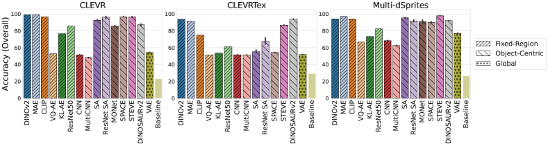
Figure 2: Average accuracies on the VQA downstream task for different upstream representation models, when using T-15 as the downstream model. The bars indicate means and 95% confidence intervals with 3 random seeds, when available.

Our key findings are presented in this section. In our main set of experiments, we assess how different model representations perform on the Visual Question Answering (VQA) downstream task defined in Section 3. We primarily focus on results from synthetic datasets where we have a unified question-generation procedure and access to underlying ground-truth factors. Our downstream models are transformer encoders with $2$, $5$, $15$, and $20$ layers, which we refer to as T-$n$ with $n$ the number of layers. We train all combinations of upstream representation models and downstream classifiers, which amounts to 852 downstream models, with the cross-entropy loss. We provide all implementation details in Appendix B and additional experimental results in Appendix E.

We conducted an extensive set of experiments with numerous baselines. Therefore, we break down the results into small points and summarize the main takeaways. In the following, we report average results and confidence intervals over 3 random seeds, except for foundation models, where only 1 seed is available. We omit MONet’s results on CLEVRTex due to its suboptimal performance, consistent with similar experimental results by Papa et al. [31]. When extending to VQA-v2, we keep only the pre-trained foundation models and top-performing OC models, excluding other upstream representation models due to their poor performance. Additionally, we report the results on VQA-v2 only with T-2 as the downstream model due to a degradation in performance observed when increasing the number of transformer layers (see Section B.3 for more details). Finally, unless explicitly mentioned, the Multi-dSprites version featured in the plots is the one comprising $320$k unique images.

4.1 Main Findings

Performance of Large Foundation Models.

Fig. 2 shows the overall accuracy for different upstream models across different synthetic datasets with T-15 as the downstream model, which generally achieves the best performance across synthetic datasets and upstream models. We observe that large foundation models, i.e., DINOv2, CLIP, and MAE, without any fine-tuning perform comparably well or the best on all datasets, although not by a large margin. However, when considering compute requirements, the picture appears more nuanced. In Fig. 3, which shows overall accuracy against the GFLOPS used for downstream training, we observe that some OC models achieve comparable performance to large foundation models with significantly less compute, making them more appealing under a limited compute budget.

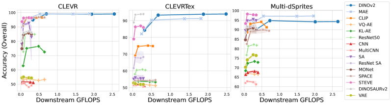
Figure 3: Average accuracies of different models w.r.t. downstream GFLOPS across different datasets. Points along the x-axis represent T-2, T-5, T-15, and T-20, respectively. For pre-trained models, only one seed is available. For other models, the results are averaged over 3 random seeds and the shaded areas indicate 95% confidence intervals.

It’s important to emphasize the differences in model sizes and training data between foundation models and OC models. As shown in Table 2 in Section B.1, STEVE and ResNet SA, which are the generally best-performing OC models excluding DINOSAURv2, are much smaller than their counterparts in the foundation model group and are specifically trained on the datasets studied in this work, which are significantly smaller than those used for training foundation models. Additionally, foundation models require substantial computational resources and significant engineering for pre-training, which are beyond our control. Therefore, carefully analyzing the effects of these factors in studies like ours can be challenging.

Effect of Object-Centric Bias.

DINOSAURv2, which consists of a pre-trained DINOv2 with Slot Attention applied downstream, allows us to explore the effect of applying the OC bias on a foundation model. Comparing the results of DINOv2 and DINOSAURv2 in Figs. 2 and 3 on CLEVRTex, the most complex and realistic synthetic dataset in our study, we observe that DINOSAURv2 outperforms all other models, including DINOv2, while requiring less downstream compute. Additionally, by looking at Fig. 14 (Section E.3) which shows the overall accuracies on different downstream model sizes, we observe that on T-2, DINOv2 exhibits inferior performance compared to DINOSAURv2 on CLEVRTex. However, as we scale up the downstream model, starting from T-5, DINOv2 almost matches DINOSAURv2. This indicates that DINOv2 representations do contain the relevant information for the downstream task, but they seem to be less explicit and less readily usable, necessitating a larger downstream model compared to DINOSAURv2 to extract the required information effectively [90].

Performance of Other Upstream Models.

In Fig. 2, a discernible pattern emerges among upstream models. Generally, OC models consistently outperform other models except large foundation models. Smaller pre-trained models (VQ-AE, KL-AE, and ResNet50) tend to perform worse. Notably, on CLEVRTex, this trend is less pronounced, as most OC and pre-trained models struggle due to the dataset’s complexity. End-to-end CNN and MultiCNN models consistently score the lowest, followed by the global representation of VAEs.

Within foundation models, DINOv2 and MAE consistently outperform others, with CLIP ranking as the third-best model probably due to its relatively smaller size. Looking at Table 2, we observe that while the good performance of DINOv2, MAE, and CLIP can likely be attributed to the size of their backbone, there appears to be no clear trend explaining the performance gap among smaller models.

Real-world Data.

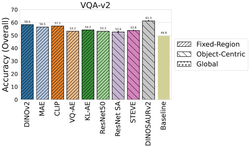
Figure 4: Average accuracies on VQA-v2 for different upstream models, with T-2 as the downstream model. The bars indicate means and 95% confidence intervals with 3 random seeds, when available.

To investigate whether our findings hold in real-world scenarios, we conduct the same experiments on the VQA-v2 dataset. To better understand the models’ performances, we replace the naive baseline with a more informative baseline trained only on questions without any information about the corresponding images. Fig. 4 shows the overall accuracy of different upstream models on VQA-v2 with T-2 as the downstream model. We observe that DINOSAURv2 significantly outperforms all other models, including DINOv2. Additionally, the performance pattern across different models is consistent with that observed in synthetic dataset experiments, supporting our main findings.

4.2 Additional Insights

Property Prediction vs VQA.

We additionally evaluate the representations on property prediction, a much simpler downstream task wherein the objective is to predict object properties from the representations. We adopt the same setup as Dittadi et al. [30] (see Section B.4 for further details). In Fig. 6, we observe a strong correlation between accuracy on this simple task and downstream VQA performance. This clearly demonstrates that models capable of accurately predicting object properties excel on more challenging tasks like VQA. Therefore, performance on simple tasks like property prediction can be a useful evaluation metric for model selection. For the complete correlation results, see Section E.1.

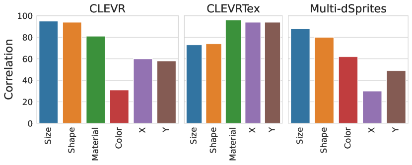
Figure 5: Correlation between property prediction accuracy (reported separately by object property) and overall VQA accuracy.

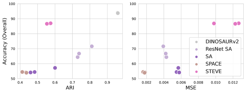
Figure 6: Overall VQA accuracy with T-15 as downstream model, plotted against ARI and MSE for different OC models on CLEVRTex.

Upstream vs. Downstream Performance.

Fig. 6 depicts the relationship between upstream performance metrics and downstream VQA accuracy of OC models when using T-15 as the downstream model on CLEVRTex. Notably, STEVE exhibits the worst reconstruction MSE among OC models but achieves the second-best accuracy on VQA. This is not necessarily surprising: while Dittadi et al. [30] observed a negative correlation between MSE and downstream performance, Papa et al. [31] later showed this to no longer hold in the presence of textured objects. However, a higher ARI was shown to be predictive of better downstream performance. This appears not to hold in our case, as ResNet Slot Attention attains the second-best ARI but does not perform well in the VQA downstream task, while STEVE has a poor segmentation performance while achieving high accuracy. Further investigations are needed to shed more light on these trends, allowing for more robust upstream model selection strategies. For additional results on more upstream metrics and other datasets, see Section E.2.

Effect of Training Size.

Fig. 8 depicts the percentage of decrease in the overall error rate of different models on Multi-dSprites when increasing the training size from $40$k to $320$k unique images. Notably, with about $8$x more data, most upstream models show similar error rate improvements, typically around 20–30%, regardless of their initial performance. STEVE stands out as the main exception, exhibiting an increase in overall error rate of up to 40%. Furthermore, the end-to-end models CNN and MultiCNN, as well as VQ-AE, show minimal improvement compared to the other models. See Section E.4 for further results, including raw accuracies and additional dataset sizes between $40$k and $320$k.

Consistency of the Results Across Question Types.

The average Spearman rank correlation between VQA accuracy on different question categories is 0.96 for CLEVR, 0.98 for CLEVRTex, 0.89 for Multi-dSprites, and 0.92 for VQA-v2. This suggests that the average VQA accuracy results shown in Figs. 2 and 4 are consistent across question categories. In Section E.5, Fig. 17 shows that these rank correlations are consistently high for all pairs of question categories, and Figs. 18, 19, 20, 21, 22, 23, 24, 25, 26 and 27 illustrate the complete VQA accuracy results separately by question category.

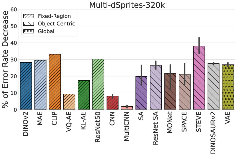
Figure 7: Average % decrease in VQA error rate for different upstream models on Multi-dSprites, when increasing the training set size from $40$k to $320$k, using T-15 as the downstream model. The bars indicate means and 95% confidence intervals with 3 random seeds.

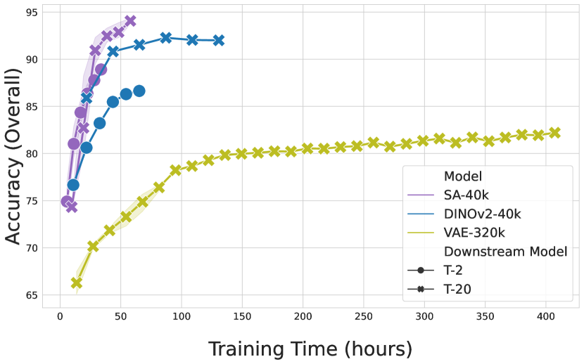
Figure 8: VQA accuracy of different models w.r.t. downstream training time on Multi-dSprites. Slot Attention and DINOv2 are trained on Multi-dSprites with 40k images, while the VAE is trained on 320k images for 3 million steps (5x more than the other models).

Delving deeper into the results for each category, it becomes apparent that on VQA-v2, Number questions, which require recognizing quantities in the image, are harder for all the models compared to Yes/No questions. On synthetic datasets, we observe that Count questions, which necessitate an understanding of the existence of multiple objects with specific properties, are generally the most challenging for almost all models. In contrast, Exist questions are the easiest, which is expected because they check for the existence of a single object with specific properties. Among Compare Integer questions, Equal questions appear to be the most challenging, requiring an exact count of two sets of objects. Finally, in Attribute questions, Size questions emerge as the easiest, while there is no specific discernible pattern among other object attributes.

Evaluation of Global Representations.

Here we further investigate whether the global representations of a VAE can match the performance of OC representations when given a significant advantage in terms of data and training budget. We continue training the largest downstream model (T-20) on top of the VAE on Multi-dSprites with $320$k unique images for $3$ million steps and compare the result with other models trained on Multi-dSprites with the smallest training size ($40$k), with the smallest downstream model (T-2) trained for the default number of training steps ($600$k).

From Fig. 8, it is evident that the performance of T-20 trained on top of the VAE cannot match the performance of T-2 trained on top of Slot Attention and DINOv2. In conclusion, even with a larger downstream model, more training steps, and a larger training dataset size, global representations of VAEs cannot match the performance of OC models and therefore do not seem ideal for downstream tasks related to objects.

5 Conclusion and Discussion

In this study, we carefully assess OC representations and compare them with foundation models and various benchmarks using three synthetic and one real-world multi-object datasets. Our focus is on the Visual Question Answering (VQA) task which requires an accurate compositional understanding of the image and the objects in it, as well as complex relational reasoning. We find that foundation models match or perform comparably to OC models without needing fine-tuning or hyperparameter adjustments. However, they are substantial in size and demand more computing budget. Overall, this points to a complex trade-off between model classes. Still, one can get the benefits of both worlds by applying the OC bias to foundation models. Furthermore, we offer various insights into VQA performance across different scenarios and its relationship with other downstream and upstream performances of the models.

While our study encompasses various widely used OC datasets, each exhibiting a noticeable range in complexity and visual attributes, only one of them consists of real-world images. A potential avenue for future exploration could involve extending our analysis to include more real-world datasets. Additionally, another possible avenue is to extend our work to videos, where understanding the scene is more challenging due to the dynamics present in the video. Furthermore, since we employ off-the-shelf foundation models, there is potential for future research to explore the effects of fine-tuning certain components or the entirety of these models, both in the presence and absence of the OC inductive bias. Lastly, a systematic exploration of the generalization capabilities of OC models or expanding our investigation into other downstream tasks, such as causal representation learning, presents intriguing possibilities for future work.

Appendix A Broader Impact

In this work, we are taking a step in the direction of systematically analyzing and understanding the reasoning capabilities of deep learning systems with a particular focus on object-centric models, which benefits both the research community and society. We do not see a negative societal impact of this work beyond what is brought about by general advances in machine learning.

Appendix B Models and Implementation Details

Here we elaborate on the upstream and downstream models included in this study along with details on the training, the implementation, and hyperparameter choices.

B.1 Upstream Models

Here we elaborate on all the upstream models we use in our experiments and provide details on the implementation, training, and hyperparameter choices.

Implementation & Training Details.

Our code is based on the implementations of object-centric models of Dittadi et al. [30] and we use their implementation of Slot Attention, MONet, SPACE, and VAE. For these models, we use the same set of recommended hyperparameters on CLEVR and Multi-dSprites, and apply the same hyperparameters for CLEVRTex as used in CLEVR. All other models are either re-implemented or adapted from available code. Unless explicitly stated otherwise, except for pre-trained foundation models, we train all the other models with a default batch size of $32$ for $3$ random seeds with Adam optimizer. The training finishes after $500$k steps on synthetic datasets and $250$k steps on COCO images of VQA-v2. The reported metrics are then averaged over the seeds to provide a comprehensive assessment. Additionally, more information about pre-trained models and the size of the models are shown in Table 2. The details of each model are explained below.

DINOv2.

DINOv2 [68], an enhanced version of the DINO [74], stands out as a self-supervised ViT-based model designed for training high-performance computer vision models without the need for extensive labeled data. It serves as a versatile backbone for diverse tasks, including image classification, video action recognition, semantic segmentation, and depth estimation. Trained on a carefully curated dataset comprising $142$ million images with a discriminative self-supervised method, DINOv2 excels in producing versatile visual features that transcend specific image distributions and tasks without the necessity for fine-tuning.

Similar to DINO, DINOv2 follows a transformer architecture, with a patch size of $14$, and is trained with $1$B parameters with a self-supervised learning objective, and distilled into a series of smaller models that generally surpass the other best available all-purpose features. There are $4$ distinct backbone versions, each varying in the number of transformer layers. After experimenting with all $4$, considering a balance between the performance and downstream training time, we selected the second-largest variant, denoted as ViT-L/14. We employ this backbone without fine-tuning, and uniformly resize images from all datasets to dimensions of $224\times 224$ and pass them to the model, generating fixed-region $16\times 16$ representations with a channel size of $1024$ for each patch. We flatten the spatial dimensions and pass a matrix of size $256\times 1024$ to the downstream model.

MAE.

The Masked Autoencoder (MAE) [69] is a simple approach for reconstructing an original signal from a partial observation. In this approach, the image is divided into non-overlapping patches, with $75$% of them randomly masked. These patches are then fed into a ViT-based encoder, which converts the partially observed input into a latent representation. Next, a lightweight decoder, which uses the representation and mask tokens, reconstructs the original image. The model is trained on ImageNet-1K [91] by minimizing the Mean Squared Error (MSE) between the reconstructed and original input in the pixel space.

There are various pre-trained MAEs available, differing in model sizes. In our framework, we utilize the pre-trained ViT-L/16. We resize the input images to $224\times 224$ and pass them to the encoder without masking. This generates a fixed-region representation sequence of length $197$ ($196$ corresponding to different regions in the image and one corresponding to the output of the CLS token) with a latent size of $1024$ for each sequence. We pass the obtained representation matrix without any modifications to the downstream model.

CLIP.

The Contrastive Language-Image Pretraining (CLIP) [70] is a multimodal model that learns to associate images and corresponding text descriptions. CLIP uses a ViT to extract a feature vector that represents the visual content of the image. Similarly, for the text, CLIP uses a transformer-based model to generate a feature vector that represents the semantic content of the text. These two feature vectors are then projected into a shared embedding space and the cosine similarity between the two vectors is calculated. The model is trained on a dataset of $400$ million (image, text) pairs collected from a variety of publicly available sources on the Internet, using a contrastive loss function which is a symmetric cross-entropy loss over the similarity scores, that encourages the similarity between the image and text feature vectors to be high when they are a matching pair and low when they are not.

In our experiments, we utilize a pre-trained CLIP image encoder with a ViT architecture denoted as ViT-B/32. Similar to DINOv2 and MAE, we resize the input images for all datasets to $224\times 224$ and pass them to the encoder. The encoder produces a representation of size $50\times 768$ (one corresponding to the output of the CLS token and the rest corresponding to regions in the image) which we utilize directly in the downstream model.

Table 2: Model sizes and training information of the models.

Model	Model Architecture	# of Params†	Pre-training Dataset	Dataset Size
DINOv2	ViT-L/14	304M	LVD-142M	142M
MAE	ViT-L/16	303M	INet-1k	1.2M
CLIP	ViT-B/32	87M	WIT-400M	400M
VQ-AE	-	34.5M	OpenImages v4	9M
KL-AE	-	34.5M	OpenImages v4	9M
ResNet50	-	23M	INet-21k	14M
CNN	-	0.1M	-	-
MultiCNN	-	1.4M	-	-
SA	-	0.9M	-	-
ResNet SA	-	22.4M	-	-
MONet	-	1.6M	-	-
SPACE	-	5.3M	-	-
STEVE	-	17.1M	-	-
DINOSAURv2∗	-	4M + 304M	-	-
VAE	-	19.2M	-	-
∗# of parameters of pre-trained DINOv2 is shown separately.
† Except for foundation models, # of parameters are reported on CLEVR.

VQ-AE & KL-AE.

VQ-AE and KL-AE are two pre-trained autoencoders of the latent diffusion model (LDM) [42]. In LDM, they don’t directly use a diffusion model in pixel space. Instead, to facilitate training on constrained computational resources without compromising quality and flexibility, they apply the models in the latent space of a powerful autoencoder pre-trained on OpenImages [92] with $9$M images in an adversarial manner. The autoencoder consists of an encoder that downsamples the images by a factor $f$, and a decoder that reconstructs the original image. In order to avoid arbitrarily high-variance latent spaces, they apply two different regularizations: one imposes a KL penalty towards a standard normal on the learned latent (KL-AE), similar to a VAE, and the other one uses a vector quantization layer [93] within the decoder (VQ-AE).

Various pre-trained autoencoders with different downsampling factors are available. In our experiments, we explore multiple models with varying downsampling factors and find that a factor of $16$ is the balancing point between performance and training speed. Therefore, we adopt models with this factor for further analysis. In our experiments, we utilize the encoder of these two autoencoders off-the-shelf. By applying the encoders, we get a vector of size $W/16\times H/16\times D_{fr}$ where $D_{fr}$ is $16$ and $8$ for KL-AE and VQ-AE, respectively. Similar to DINOv2, we flatten $2$d feature maps and feed them into the downstream model.

ResNet50.

ResNet50 [71] is a deep neural network with 50 layers that has been pre-trained on ImageNet-21k [91]. It is well-known for its residual learning blocks and serves as a baseline in our study. In our experiments, we employ the off-the-shelf ResNet50 model and remove the pooling and fully connected layers at the end. We apply the default ResNet50 transformations on the input image, pass it to the model, and obtain a vector of size $W/32\times H/32\times 2048$ which we flatten the spatial dimensions and pass to the downstream model.

CNN.

CNN [72] is a small convolutional neural network that is commonly used in the literature. It consists of a few convolutional layers with ReLU activation functions in between, and is trained end-to-end with the downstream model on the downstream task. It produces a fixed-size fixed-region representation of size $4\times 4\times 64$ which we flatten the spatial dimensions and produce a vector of size $16\times 64$ and pass it to the downstream model. The hyperparameters of CNN are shown in Table 3.

MultiCNN

MultiCNN [57] is an object-centric model consisting of $N_{slots}$ CNNs, each dedicated to detecting a single object within an image. These CNNs operate with non-shared parameters, processing each input image independently. MultiCNN shares the same dataset-specific hyperparameters as the CNN baseline, and similar to CNN, it is trained end-to-end using the same training hyperparameters and loss function as the downstream model. The output of each CNN undergoes complete flattening, followed by a shared linear layer of size $64$, resulting in a representation of size $N_{slots}\times 64$, which is then passed to the downstream model.

Table 3: Hyperparameters of CNN.

CNN
Dataset	Kernel Size	Stride	Output Channels	Activation Function
CLEVR & CLEVRTex	8	4	32	ReLU
	4	2	64	ReLU
	4	2	64	ReLU
	3	1	64	ReLU
Multi-dSprites	8	4	32	ReLU
	4	2	64	ReLU
	3	1	64	ReLU

Slot Attention.

Slot Attention [2] has become the primary representative for object-centric (OC) learning in recent years. It follows an autoencoder setup and begins with a Convolutional Neural Network (CNN) and is followed by the Slot Attention module. This module refines the initial image features through multiple iterations, turning them into distinct slots representing objects. Each slot is updated using a Gated Recurrent Unit (GRU) that takes the current slot and attention information as inputs. After refining, these slots are used to reconstruct the appearance and mask of each object, which are then combined to reconstruct the original image. The model is trained by minimizing the MSE reconstruction loss.

We also employ an improved version of Slot Attention introduced in Biza et al. [61] which we refer to as ResNet SA. In this improved version, the CNN backbone is replaced by a ResNet34 [71] without pre-training, and a larger feature map resolution of $16$ on synthetic datasets and $7$ on VQA-v2 is used in both the encoder and the decoder of the model. Furthermore, the initial slots are changed into learnable slots. Both the original and improved models are trained on each dataset with a batch size of $64$, a learning rate of $0.0004$, a learning rate warmup of $10$k steps, and an exponential learning rate decay with a half-life of $100$k steps. For ResNet SA, we additionally clip the gradient norm at $0.05$ to stabilize training. We follow the same architecture for ResNet SA as in Biza et al. [61] on synthetic datasets. On VQA-v2, we modify the architecture by replacing the initial convolutional layer of ResNet34 with a convolutional layer featuring a kernel size of $7\times 7$ and a stride of $4$. Additionally, in the decoder, we incorporate two additional transpose convolutional layers at the beginning, each configured with the same hyperparameters as the existing transpose convolutional layers. After training, the learned slot vectors of size $N_{slots}\times 64$ are used as representations in the downstream model for both versions.

MONet.

The Multi-Object Network (MONet) [4] consists of a recurrent segmentation network that generates attention masks that represent the probability of each pixel belonging to each object. For each slot, a VAE (the component VAE) encodes the image and the current attention mask, and decodes the latent representation to an image reconstruction of the slot and the slot mask. To create the final reconstructed image, the reconstructed images are combined using the attention masks obtained from the segmentation network. The model is trained by an objective function comprising a reconstruction loss defined as the negative log-likelihood of a spatial Gaussian mixture model (GMM) with one component per slot, where each pixel is modeled independently, and a KL divergence of the component VAE, and an additional mask reconstruction loss for the component VAE. The mean of the GMM for each component is used as the representation of each object. The learned representation is a vector of size $N_{slots}\times 16$ and is directly used for the downstream task.

SPACE.

Spatially Parallel Attention and Component Extraction (SPACE) [3] provides a unified probabilistic modeling framework that combines the best of spatial attention and scene-mixture approaches. Foreground objects are identified using bounding boxes computed in a parallel spatial attention process, and background elements are modeled using a mixture of components. The model is trained by optimizing the Evidence Lower Bound (ELBO) of the probabilistic model. An additional boundary loss is introduced to penalize the splitting of objects across bounding boxes, addressing potential under- or over-segmentation issues. SPACE representations are vectors of size $69\times 38$ where $69$ is the number of slots that is determined by the grid size, and the latent representation of each slot is obtained by concatenating all the latent variables which will have a dimension of $38$. We utilize this representation directly in the downstream model.

Table 4: Hyperparameters of STEVE.

STEVE
Module	Hyperparameter	Hyperparameter Value
Encoder	Corrector Iterations	2
	Slot Size	192
	MLP Hidden Size	192
	# Predictor Blocks	1
	# Predictor Heads	4
	Learning Rate	0.0001
Transformer Decoder	# Decoder Blocks	8
	# Decoder Heads	4
	Hidden Size	192
	Dropout	0.1
	Learning Rate	0.0003
DVAE	Learning Rate	0.0003
	Patch Size	4 $\times$ 4 pixels
	Vocabulary Size	4096
	Temperature Start	1.0
	Temperature End	0.1
	Temperature Decay Steps	30k

STEVE.

STEVE [6] is a simple object-centric video model achieving remarkable performance over various complex and naturalistic videos. It is a more robust version of SLATE [5], a state-of-the-art object-centric model. The model contains two reconstruction paths. The first path uses a discrete VAE encoder to convert the input image into discrete tokens, and then a discrete VAE decoder to reconstruct the original image. This path is trained using MSE reconstruction loss. The second path uses a CNN-based image encoder on the input, and the output is fed into a recurrent slot encoder that updates slots over time using recurrent neural networks. Finally, a slot-transformer decoder, similar to SLATE, is applied to the produced slots to predict and reconstruct the discrete tokens of the input image. This path is trained by minimizing the cross-entropy loss between the original tokens produced by the discrete VAE encoder, and the predicted tokens of the slot-transformer decoder.

We incorporate the original implementation of STEVE into our framework. STEVE works on videos, considering the input to be a sequence of $t$ image frames. Following the authors’ recommendation, to utilize it on images, we treat images as $1$-frame videos and pass them to the model. On synthetic datasets, we train STEVE for $500$k steps with an exponential learning rate decay with a half-life of $250$k steps and with $30$k warm-up steps. For VQA-v2, we employ the same training hyperparameters but reduce the number of steps to $250$k. After the training, we use slots of size $N_{slots}\times 192$ obtained from the recurrent slot encoder in the downstream model.

A summary of the model’s hyperparameters on all datasets is shown in Table 4. We maintain the original architecture for the CNN backbone and discrete VAE encoder/decoder for synthetic datasets. However, for VQA-v2 with image sizes of $224\times 224$, we reduce the feature map dimensions of both the discrete VAE encoder and CNN backbone by half. This adjustment includes changing the stride of the first convolutional layer of the CNN backbone to $4$. Additionally, in the discrete VAE encoder, we insert a convolutional layer with a $2\times 2$ kernel and stride $2$, followed by ReLU activation, after the initial convolutional layer. To accommodate these feature map changes in the discrete VAE decoder, we duplicate the four convolutional blocks and the pixel shuffling layer before the final convolutional block.

It is noteworthy that the training of STEVE is not entirely stable, as we observed that upstream performance metrics begin to degrade after some training time (after roughly 20-40k steps). However, when training the model for longer, we observe that it performs well on the downstream task. Nevertheless, in some seeds, the training fails as the upstream metrics are significantly worse than in other seeds. Therefore, we only consider the seeds that are stable and perform the best in terms of reconstruction and segmentation quality.

Additionally, we experimented with a modified version of STEVE using a pre-trained DINOv2 as the CNN encoder backbone. However, it performed similarly or worse than the original STEVE on the downstream VQA. We suspect this may be due to the chosen hyperparameters or an architectural bottleneck in the discrete VAE. As a result, we decided not to include it in our reported results.

Table 5: Hyperparameters of DINOSAURv2.

DINOSAURv2
Hyperparameter		CLEVR, CLEVRTex	VQA-v2
		& Multi-dSprites	(COCO)
Training Steps		500k	250k
Batch Size		64	64
LR Warmup Steps		10k	10k
Peak LR		0.0004	0.0004
Exp. Decay Half-Life		100k	100k
ViT Architecture		ViT-L	ViT-L
Patch Size		14	14
Feature Dim.		1024	1024
Gradient Norm Clipping		1.0	1.0
Image Size		224	224
Cropping Strategy		Full	Full
Image Tokens		256	256
Decoder	Type	MLP	MLP
	Layers	4	4
	MLP Hidden Dim.	512	2048
Slot Attention	Iterations	3	3
	Slot Dim.	256	256
	MLP Hidden Dim.	1024	1024

DINOSAUR.

DINO and Slot Attention Using Real-world data (DINOSAUR) [7] is an object-centric model designed to bridge the gap between object-centric models and real-world data. It consists of an encoder that extracts features from the input data, a slot attention module that groups the extracted features into slots, and a decoder that reconstructs the extracted features. Their approach can be considered similar to SLATE [5] and STEVE [6], but with the difference of reconstructing global features from a pre-trained Vision Transformer [94] instead of local features from a VQ-VAE [93].

We adapt the original implementation of DINOSAUR into our framework and replace the pre-trained DINO backbone with pre-trained DINOv2 [68], which we refer to as DINOSAURv2. Similar to the original training procedure of DINOSAUR, the input images are resized to $224\times 224$ and we train DINOSAURv2 for $500$k steps on synthetic datasets and $250$k steps on COCO images of VQA-v2. The training uses a learning rate of $0.0004$, a learning rate warm-up of $10$k optimization steps, and an exponentially decaying learning rate schedule. Furthermore, we clip the gradient norm at $1$ to stabilize training. After the training, we use the slots of size $N_{slots}\times 256$ obtained from the Slot Attention module in the downstream model. The full hyperparameters of the model are provided in Table 5.

VAE.

We train a variational autoencoder (VAEs) [77] with a broadcast decoder [73] as a baseline that learns global representations. We use the broadcast VAE implementation of Dittadi et al. [30] with the same architecture and hyperparameter choices. For CLEVRTex, we use the same hyperparameters as in CLEVR. The latent size is selected to be $64$ times the number of slots used when training an object-centric model on the same dataset. As explained in Section 3.5, we divide the flat representation vector into $N_{slots}$ vectors of size $64$, and pass them to the downstream model.

B.2 Text Embedding Module

As our text embedding module, we use Text-to-Text Transfer Transformer (T5) [86], a transformer-based language model developed by Google AI Language. It is capable of performing a wide range of natural language processing tasks such as text classification, question answering, summarization, and translation. The model is trained on the colossal, cleaned version of Common Crawl’s web crawl corpus (C4), an 806-gigabyte corpus of text data using a pretext task called Text-to-Text Transfer Transformer (T5), which involves converting a given input text to a target output text. We utilize the available implementation in Hugging Face’s Transformers library. T5 comes in different sizes and we use the T5-base tokenizer and encoder which produces the representations of size $768$ for each token.

B.3 Downstream VQA Setup

Architecture and Hyperparameters.

We use a transformer-based architecture [89] which is the standard downstream architecture for the VQA task [12, 87, 88]. We utilize the original PyTorch implementation of the transformer. We first project the image and the text representations with two separate linear layers with a $126$ size and a dropout of $0.1$. Then, we augment the image and text vectors with a $2$-dimensional one-hot vector indicating whether the input is from the image representation or the text embeddings. A sinusoidal positional encoding is then added to the text embeddings. We introduce a trainable vector $\textit{CLS}\in\mathbb{R}^{128}$, akin to the CLS token in BERT [87], to generate classification results. The image and text representations, along with the CLS token, are concatenated and passed through a transformer encoder with a d_model of $128$ and a hidden dimension of $128$. The transformed value of the CLS token is passed through a classifier MLP that generates a probability vector over all possible answers in each dataset. The MLP consists of $2$ linear layers of size $128$. A normalization layer, a dropout of $0.1$, and a ReLU activation function are applied in between the layers.

Training.

On synthetic datasets, all downstream models are trained with a batch size of $128$ and a learning rate of $0.0001$ for $600$k training steps, with the cross-entropy loss. However, when using DINOv2 and MAE as upstream models, it is infeasible to keep the current batch size with only one GPU due to the substantial sequence length of the representations. To ensure a fair comparison, gradients are accumulated, and the optimizer is applied every $4$ training step with a reduced batch size of $32$. Consequently, the downstream model is trained for $2.4$ million steps, $4$ times the default number of steps.

On VQA-v2, we train all downstream models with a batch size of $32$ for $300$k steps, using the same loss function as for synthetic datasets. Furthermore, we use a learning rate of $0.0001$ for T-2 and T-5, and $0.00005$ and $0.00001$ for T-15 and T-20, respectively. However, we find that T-2 outperforms the other downstream models, with performance degrading significantly as the number of layers increases which is due to overfitting caused by the much smaller training size of VQA-v2 compared to other datasets in our study. As a result, we only report results for T-2 on VQA-v2.

B.4 Downstream Property Prediction Setup

Here we assess representations by training downstream models to predict ground-truth object properties from these representations. Following the approach outlined by Dittadi et al. [30] for object property prediction on synthetic datasets. in summary, we employ a single downstream model $f$ to predict the properties of each object independently. To be more specific, for OC models, we apply $f$ on each slot representation, i.e. $\hat{y}_{k}=f(z_{k})$, where $z_{k}$ is the $k$th slot representation and $\hat{y}_{k}$ is the predicted properties of the $k$th slot. Similarly, for models with fixed-region representations, we treat each region as a slot and apply the same approach as with OC models. We find this approach to be effective for these models. Lastly, for models with global representations, since the representations of individual objects are not readily available, we adopt the same strategy as demonstrated in Dittadi et al. [30] which has proven to be working. We predict the properties of all objects using the downstream model $f$ and split it into $K$ vectors $\{\hat{y}_{k}\}_{k=1}^{K}$ where $K$ roughly corresponds to the number of slots in an OC model.

Since the predicted properties might not correspond to the objects in the same order as the ground-truth objects, and the number of slots can exceed the number of objects in the image, we follow Dittadi et al. [30], Locatello et al. [2] in using the same loss-matching algorithm to match $\hat{y}_{k}$ with its corresponding ground-truth vector. We define $f$ as an MLP with $1$ hidden layer of size $256$, and we utilize cross-entropy loss for categorical properties and MSE for numerical properties. We train $f$ for one seed on $10000$ images of each dataset using Adam optimizer with a learning rate of $0.001$ and a batch size of $64$ for $6000$ steps. For a randomly selected test set of $2000$ images, we calculate the accuracy for categorical properties and the adjusted $R^{2}$ for numerical properties and report the results.

Appendix C Datasets

We work with $3$ existing multi-object datasets: Multi-dSprites, CLEVR, and CLEVRTex. We use the common format for these datasets as outlined in Dittadi et al. [30]. We primarily focus on these datasets due to their unified question-generation procedure and complete access to all underlying ground-truth object properties. Additionally, we utilize VQA-v2 to extend our study to real-world settings. All datasets are summarized in Table 6. More details about each dataset are provided in the next subsections.

C.1 Overview of Datasets

CLEVR

CLEVR [44] comprises $128\times 128$ images depicting $3$D scenes with a plain gray background featuring up to $10$ objects that may partially occlude one another. Objects vary in colors ($8$ options in total), materials (rubber or metal), shapes (sphere, cylinder, cube), sizes (small or large), and positions (x and y) as well as rotations. Following previous works [2, 30, 80], we utilize the CLEVR6 variant to learn object-centric representations in which the number of objects is limited to $6$. The dataset has been cropped and resized according to the procedure detailed originally by Burgess et al. [4].

CLEVRTex

The CLEVRTex dataset extends the original CLEVR [44] by incorporating textures on object surfaces, introducing a more visually complex environment. Each scene in CLEVRTex consists of $3$-$10$ objects with distinct shapes (cube, cylinder, sphere, monkey head), sizes (small, medium, large), and textures ($60$ in total), contributing to the diversity of visual features. The backgrounds also present complex textures compared to the plain gray ones in CLEVR. The dataset is designed to facilitate the exploration of models’ abilities in handling textured objects, providing a valuable resource for evaluating the performance of vision-related tasks in the context of rich visual scenes.

Multi-dSprites

This dataset is derived from the dSprites dataset [79] of $64\times 64$ synthetic images. Following prior research [30, 2, 80], we utilize the Multi-dSprites variant, featuring colored sprites set against a grayscale background where the intensity of the uniform grayscale background is randomly determined for each image. Each scene consists of $2$–$5$ objects with randomized attributes, including shapes (ellipse, square, heart), sizes (selected from $6$ discrete values in $[0.5,1]$, and converted to small and large with a threshold of $0.8$), x and y positions, orientation, and color (randomly sampled in HSV space). Objects might occlude one another, with certain objects being nearly entirely concealed by others in specific images. Consequently, we eliminate images where an object is significantly obscured by another object, leaving only those with clearer visibility of individual objects. We use $4$ different training sizes of this dataset which is demonstrated in Table 6.

VQA-v2

VQA-v2 [82, 43] pairs open-ended questions with images from the MS COCO 2014 dataset [83]. It serves as a benchmark for evaluating how well models can comprehend and reason about visual information in real-world scenarios. The questions cover a wide range of topics and require a detailed understanding of the image content, spanning from basic inquiries about object presence to more complex queries about relationships and attributes within the scene. Answers are categorized into Yes/No, Number, and Other types. Each question has 10 ground-truth answers, with the most frequent ground-truth answer considered correct in our evaluation framework. We filter out specific questions in the dataset based on their answer type, as explained in detail in Section C.2. We train downstream models using the filtered train split of the dataset. However, since answer types for the test split are not available, we cannot apply the same filtering process to evaluate on this split properly. Therefore, we utilize the val split as our test set for evaluation, and additionally select a subset of $10$k questions from it as our validation set during training.

The MS COCO (Microsoft Common Objects in Context) dataset [83] is a widely used collection of images designed for object detection, segmentation, and captioning tasks. It contains images sourced from everyday scenes that are diverse in content, encompassing various objects, activities, and environments. The dataset includes over $200$k labeled images across $80$ object categories, such as people, animals, vehicles, and indoor objects, with a significant emphasis on diversity in scenes and object appearances. Following Seitzer et al. [7], we resize all the images to $224\times 224$ without any cropping, while ignoring the aspect ratio. We use the original split of the dataset when training and evaluating the upstream models. Furthermore, during upstream training, we augment the dataset by horizontally flipping images with a probability of $0.5$.

Table 6: Dataset splits for upstream and downstream training, number of slots used in training slot-based object-centric models, and count of unique answers to questions in each dataset.

Dataset Name	Slots∗	Answers	Dataset Splits†
			Train Size	Validation Size	Test Size
CLEVR6	$7$	$24$	$2314980$ ($49000$)	$70702$ ($1500$)	$70997$ ($1500$)
CLEVRTex	$11$	$20$	$1489005$ ($40000$)	$55977$ ($1500$)	$55646$ ($1500$)
Multi-dSprites‡	$6$	$22$	$1545444$ ($320000$)	$57816$ ($1500$)	$57557$ ($1500$)
			$3089425$ ($320000$)	$57540$ ($1500$)	$57557$ ($1500$)
			$6181799$ ($320000$)	$58289$ ($1500$)	$57557$ ($1500$)
			$12365042$ ($320000$)	$57792$ ($1500$)	$57557$ ($1500$)
VQA-v2 (COCO)	7	17	215553 (82753)	10000 (10000)	103717 (40504)
∗ We define it as the maximum number of objects plus one additional slot for the background.
† The values in parentheses denote the size of the corresponding image split used for the upstream model.
‡ For Multi-dSprites, We use $4$ different training sizes.

C.2 Question Generation & Preprocessing

Synthetic.

Originally, excluding CLEVR, the synthetic datasets exclusively comprise images without associated questions. Consequently, for their transformation into Visual Question Answering (VQA) datasets, we employ a question generation mechanism based on Johnson et al. [44], adapted for all datasets. The process involves utilizing a script that takes as input a JSON file that contains scene information and object features in the dataset. The script outputs a JSON file containing questions for each image. To generate questions for each image, there are $9$ different question templates that take the features of the objects in each image and generate a question based on the template. These templates are adjusted for each dataset, producing a maximum of $50$ questions for each image in each dataset. However, due to some images featuring only a few objects, the average number of questions per image tends to be less than $50$ in each dataset. Additionally, we refrain from utilizing pre-existing questions for CLEVR. Instead, we generate questions for it to establish a standardized question-generation process for all datasets.

Question templates can be categorized into $5$ categories:

1. Counting: Counting questions ask for the number of objects meeting specific criteria (e.g. “How many other things are there of the same size as the tiny metal block?”).

2. Existence: Existence questions ask if an object with certain properties is present in the image (e.g. “Are there any other things that are the same color as the cylinder?”).

3. Integer Comparison: Integer comparison questions ask about the relative sizes of two sets of objects (e.g. “Are there fewer spheres than large cylinders?”).

4. Comparing Attributes: Attribute comparison questions check if two objects have the same value for an attribute (e.g. “Do the red cube and the green cylinder have the same size?”).

5. Querying Attributes: Query questions ask about an attribute of a particular object (e.g. “What shape is the object at the right of the green cube?”).

The set of possible answers includes yes, no, numerical values between $0$ and the maximum number of objects in the dataset, and all possible values of object properties. We have a different number of templates per each question category in our question-generation process. The proportion of each question category in each dataset is outlined in Fig. 9.

Figure 9: Distribution of question categories per dataset.

For CLEVR, questions are generated based on the attributes of each object, including shape, color, size, material, and their relative position in comparison to other objects. In the case of Multi-dSprites, where objects lack a material attribute, questions focus on the shape, color, size, and relative position of the objects. Regarding CLEVRTex, questions are generated considering only shape, size, and relative position, as color is absent in the dataset and is replaced with $60$ materials, each having a specific color. The material is not included as a feature for the questions because the names of the materials are not suitable for accurate processing by a text embedding module.

Real-World.

The VQA-v2 dataset includes questions from three categories: Yes/No, Number, and Other, with open-ended answers that are not limited to specific words or numbers. Therefore, in order to use the same framework employed for synthetic datasets, we only keep a subset of questions with specific answers. We omit questions with "Other" answer types and keep "Yes/No" questions that have "yes" or "no" answers. Additionally, we retain questions with numerical answers ranging from $0$ to $14$, resulting in a total of $17$ possible answers in the "Yes/No" and "Number" categories. Before filtering, the train and test sets contain 443,757 and 214,354 questions, respectively. After filtering, they are reduced to 215,553 and 103,717.

Appendix D Metrics

Upstream.

To evaluate the performance of upstream models trained on the datasets used in our study, we use MSE reconstruction error and Adjusted Rand Index (ARI) [84], which are two commonly used metrics in the literature [2, 30, 6, 61]. Consistent with prior work, we calculate the ARI considering only foreground objects. Additionally, following Dittadi et al. [30], we include Segmentation Covering [85] and mean Segmentation Covering [50] as evaluation metrics. For more information on the upstream metrics, we refer to Dittadi et al. [30].

Downstream VQA.

To assess the performance of representations in the VQA downstream task, following previous works on applying the VQA task to object-centric models [12, 13, 44] and other works on VQA in general [43, 82, 95, 96], we use accuracy as our main metric. We also analyzed balanced accuracy which takes into account the class imbalances and is defined as the average of recall obtained in each class, and F1 score as alternative metrics but our results revealed consistent trends across all metrics. Consequently, we focus on presenting results based on the accuracy metric.

Appendix E Additional Results

In this section, we report additional results that did not fit into the main part.

E.1 Property Prediction vs VQA

Fig. 10 shows Spearman’s rank correlation between downstream property prediction performance of the models for each property, and downstream VQA performance for each question category. Overall, we observe a strong correlation between the performance of the models in two downstream tasks. It’s important to note that training for property prediction takes significantly less time than VQA, by around $2$ orders of magnitude. Hence, property prediction can be a helpful guide when selecting a model for a downstream task.

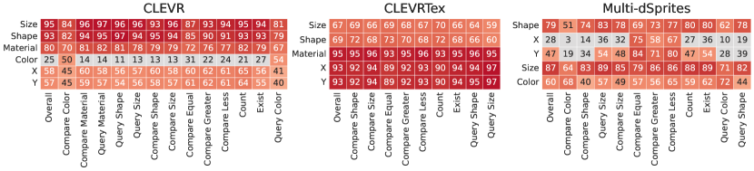
Figure 10: Spearman’s rank correlation between downstream property prediction performance and downstream VQA performance of the models. The correlations are color-coded only when $p<0.05$.

E.2 Upstream vs Downstream Performance

Here we analyze the relationship between the upstream and downstream VQA performance of OC models. We exclude VQA-v2 results due to only having three well-performing OC models for this dataset. Figs. 11, 12 and 13 depict the upstream performance of object-centric models in comparison to their downstream performance when using T-15 as the downstream model. Generally, there is no strong correlation between the two performances, and several outliers are observed in each plot.

More specifically, on CLEVR and Multi-dSprites, only ARI on CLEVR shows a slight correlation with VQA accuracy. All other upstream metrics do not correlate with the downstream performance. On CLEVRTex, however, we observe a weak correlation between ARI, mSC, and SC with VQA accuracy. At the same time, contrary to expectations, we observe a positive correlation between MSE and overall VQA accuracy which suggests that models with higher MSE values tend to perform better on the downstream task. These require further investigation which is beyond the scope of this work.

Additionally, when we look at the outliers, STEVE is the main one among OC models in all datasets, showing higher MSE and lower ARI, but better downstream performance. Also, one seed of STEVE tends to perform poorly in upstream metrics but achieves a downstream performance comparable to other seeds. Moreover, DINOSAURv2 consistently performs poorly on mSC and SC across all datasets despite performing well downstream. Additionally, SPACE typically has the best MSE but the worst downstream performance.

In conclusion, we observe that upstream metrics are not a good indicator of the downstream performance of different models and thus, are not reliable for upstream model selection.

It is noteworthy that DINOSAURv2 does not reconstruct the input but instead reconstructs the latent features of the input. Thus, it is not included in the plots showing reconstruction MSE. Furthermore, we also calculated the Spearman rank correlations between upstream and downstream metrics but due to the high p-value of most of the correlations, we chose not to report them.

Figure 11: Upstream performance of object-centric models against the overall VQA accuracy when using T-15 as the downstream model on CLEVR.

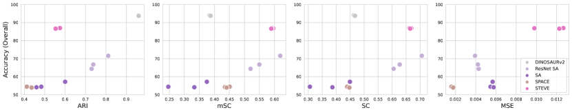
Figure 12: Upstream performance of object-centric models against the overall VQA accuracy when using T-15 as the downstream model on CLEVRTex.

Figure 13: Upstream performance of object-centric models against the overall VQA accuracy when using T-15 as the downstream model on Multi-dSprites.

E.3 Effect of Downstream Model Size

Fig. 14 depicts the overall accuracy of the models across different datasets with a downstream model having a varying number of layers. The downstream performance increases with the downstream model size but after T-15, downstream performance remains almost the same. However, on CLEVR, we see a different trend on Slot Attention, and from T-15 to T-20, the accuracy drops considerably which might be mainly because of the relative simplicity of the dataset.

Figure 14: Average accuracies of different models w.r.t. downstream model size across different datasets. For pre-trained models, only one seed is available. For other models, the results are averaged over 3 random seeds and the shaded areas indicate 95% confidence intervals.

E.4 Effect of Training Size

Fig. 15 depicts the overall accuracy of different models on Multi-dSprites with varying training sizes of $40$k, $80$k, $160$k, and $320$k unique images, and Fig. 16 shows the average percentage of decrease in error rate when increasing the dataset size from $40$k to the respective size. With increased data, most upstream models show similar performance improvement across different training sizes regardless of their initial performance. STEVE is the only exception, showing a decrease in overall error rate of up to 50%. Furthermore, the performance of the end-to-end CNN and MultiCNN models show minimal improvement compared to the other models.

Figure 15: Average accuracies on the VQA downstream task for different models on Multi-dSprites with different training sizes when using T-15 as the downstream model. The bars indicate means and 95% confidence intervals with 3 random seeds.

Figure 16: Average % decrease in VQA error rate for different upstream models on Multi-dSprites, when increasing the training size from $40$k to larger sizes, using T-15 as the downstream model. The bars indicate means and 95% confidence intervals with 3 random seeds.

E.5 Consistency of the Results Across Different Question Types

Fig. 17 shows the Spearman’s rank correlation between the performances of models on each question category when using T-15 for synthetic datasets and T-2 for VQA-v2. Additionally, Figs. 18, 19, 20, 21, 22, 23, 24, 25, 26 and 27 illustrate the accuracy of different question types of all upstream model representations across different datasets. We observe strong correlations between the performance of different question categories which indicates that the trend in the overall accuracy in Fig. 2 matches the trend in the accuracy of each question category and the results are consistent across different question categories.

Figure 17: Spearman’s rank correlation of model performances for each question category using T-15 as the downstream model.

Figure 18: Average accuracies of Exist questions for different upstream representation models when using T-15 as the downstream model. The bars indicate means and 95% confidence intervals with 3 random seeds.

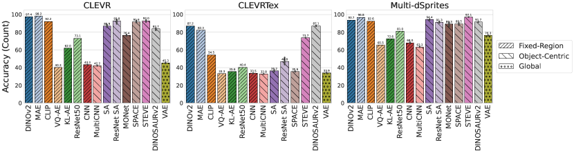
Figure 19: Average accuracies of Count questions for different upstream representation models when using T-15 as the downstream model. The bars indicate means and 95% confidence intervals with 3 random seeds.

Figure 20: Average accuracies of Compare Integer (Less) questions for different upstream representation models when using T-15 as the downstream model. The bars indicate means and 95% confidence intervals with 3 random seeds.

Figure 21: Average accuracies of Compare Integer (Greater) questions for different upstream representation models when using T-15 as the downstream model. The bars indicate means and 95% confidence intervals with 3 random seeds.

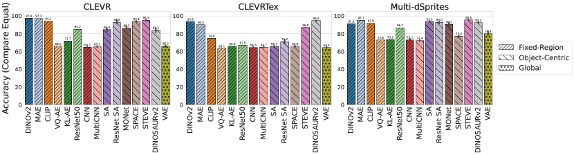
Figure 22: Average accuracies of Compare Integer (Equal) questions for different upstream representation models when using T-15 as the downstream model. The bars indicate means and 95% confidence intervals with 3 random seeds.

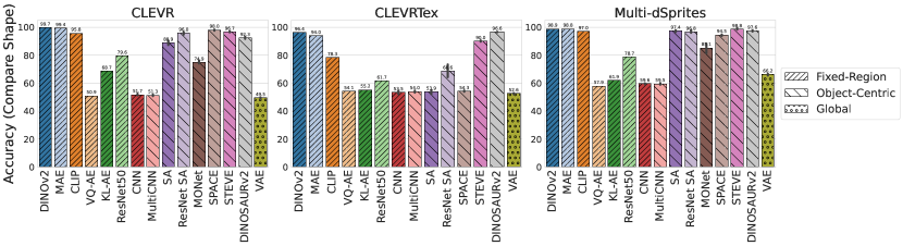
Figure 23: Average accuracies of Compare Attribute (Shape) questions for different upstream representation models when using T-15 as the downstream model. The bars indicate means and 95% confidence intervals with 3 random seeds.

Figure 24: Average accuracies of Compare Attribute (Size) questions for different upstream representation models when using T-15 as the downstream model. The bars indicate means and 95% confidence intervals with 3 random seeds.

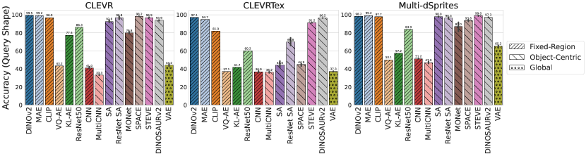
Figure 25: Average accuracies of Query Attribute (Shape) questions for different upstream representation models when using T-15 as the downstream model. The bars indicate means and 95% confidence intervals with 3 random seeds.

Figure 26: Average accuracies of Query Attribute (Size) questions for different upstream representation models when using T-15 as the downstream model. The bars indicate means and 95% confidence intervals with 3 random seeds.

Figure 27: Average accuracies of different question types for different upstream representation models when using T-2 as the downstream model on VQA-v2. The bars indicate means and 95% confidence intervals with 3 random seeds.

E.6 Full Results

The complete VQA accuracies of different upstream models across all datasets are presented in Tables 7, 8, 9, 10, 11, 12 and 13.

Table 7: Average accuracies on CLEVR when using T-15 as the downstream model. For pre-trained models, only one seed is available. For other models, the results are aggregated over 3 random seeds.

Model	Overall	Exist	Count	Compare Integer			Compare Attribute				Query Attribute
				Less	Greater	Equal	Shape	Color	Material	Size	Shape	Color	Material	Size
DINOv2	98.9	99.4	97.4	99.2	98.9	97.4	99.7	100.0	97.4	99.6	99.5	99.7	99.3	99.8
MAE	99.0	99.3	98.2	99.5	99.0	97.3	99.4	99.9	98.2	99.2	99.2	99.6	99.5	99.7
CLIP	96.5	97.9	92.2	97.7	96.8	94.1	95.8	98.6	96.2	98.0	96.9	98.2	98.1	99.1
VQ-AE	52.7	64.3	40.3	75.8	73.9	66.0	50.9	52.1	49.9	56.6	43.2	33.2	58.5	65.5
KL-AE	76.5	83.5	62.0	84.2	82.0	71.7	68.7	80.0	75.6	80.6	77.4	77.4	84.6	84.9
ResNet50	85.4	91.2	73.1	93.2	92.4	85.2	79.6	85.1	82.3	92.0	86.3	84.9	89.6	94.7
CNN	51.6	64.0	43.3	75.2	73.2	64.7	51.7	53.2	51.3	53.8	41.0	21.1	59.0	62.9
MultiCNN	48.1	64.0	42.2	74.8	72.2	65.3	51.3	52.7	51.4	53.1	33.3	12.6	50.3	52.9
SA	92.5	95.3	86.9	94.9	92.3	84.6	88.9	93.7	92.7	96.4	92.6	93.5	95.8	97.6
ResNet SA	96.2	97.6	92.8	97.3	95.9	93.0	96.0	96.4	96.3	98.5	96.8	96.4	98.0	98.7
MONet	85.7	90.3	76.4	92.9	92.3	86.3	74.9	88.0	87.9	91.5	79.8	86.1	92.2	93.6
SPACE	96.8	98.3	91.6	97.7	97.1	93.9	98.0	98.0	97.5	98.2	98.2	98.5	98.8	98.9
STEVE	96.5	97.7	93.0	98.3	97.7	95.3	96.7	96.9	96.2	98.4	96.9	96.5	97.7	98.8
DINOSAURv2	87.0	89.9	83.7	93.0	92.0	84.3	92.3	73.4	92.2	94.9	93.9	60.1	94.8	96.3
VAE	54.5	65.6	45.3	76.1	74.6	66.2	49.5	52.2	52.6	57.2	44.2	32.6	63.2	65.6

Table 8: Average accuracies on CLEVRTex when using T-15 as the downstream model. For pre-trained models, only one seed is available. For other models, the results are aggregated over 3 random seeds.

Model	Overall	Exist	Count	Compare Integer			Compare Attribute		Query Attribute
				Less	Greater	Equal	Shape	Size	Shape	Size
DINOv2	93.8	97.1	87.2	97.6	96.7	93.6	96.4	96.2	97.1	96.7
MAE	91.1	95.4	82.3	96.5	95.4	90.0	94.0	94.5	94.7	95.8
CLIP	75.1	87.1	54.5	87.1	85.9	74.8	78.3	81.9	81.9	85.6
VQ-AE	51.5	69.6	33.3	73.3	73.0	63.1	54.1	58.8	37.1	48.7
KL-AE	53.5	71.7	35.6	75.1	74.3	65.9	55.2	58.5	41.7	49.7
ResNet50	60.8	75.8	40.4	79.4	78.5	67.0	61.7	65.2	60.2	65.2
CNN	51.7	71.0	33.5	74.5	73.9	64.5	53.5	57.6	36.9	47.4
MultiCNN	51.3	70.8	32.8	74.9	73.5	64.7	54.0	57.6	36.2	46.2
SA	55.3	73.0	36.2	76.5	75.5	65.7	53.9	60.6	44.0	57.0
ResNet SA	67.6	81.7	46.8	82.3	81.0	71.2	68.6	73.7	69.8	76.9
SPACE	54.2	71.9	35.6	75.7	74.8	65.8	54.3	58.7	44.9	52.3
STEVE	86.8	93.7	73.7	93.9	92.7	86.9	90.0	92.3	91.2	93.5
DINOSAURv2	93.9	97.3	87.1	97.5	97.2	94.6	96.6	96.0	96.5	96.8
VAE	51.9	69.7	33.9	74.9	74.1	64.4	52.6	57.5	37.3	49.5

Table 9: Average accuracies on Multi-dSprites with $40$k unique training images when using T-15 as the downstream model. For pre-trained models, only one seed is available. For other models, the results are aggregated over 3 random seeds.

Model	Overall	Exist	Count	Compare Integer			Compare Attribute			Query Attribute
				Less	Greater	Equal	Shape	Color	Size	Shape	Color	Size
DINOv2	91.9	94.1	91.3	96.4	96.1	91.7	96.9	80.8	94.1	97.6	77.4	96.1
MAE	95.9	96.9	95.2	98.1	98.2	94.8	98.2	91.0	96.7	98.8	89.9	98.2
CLIP	88.4	91.0	86.6	92.8	93.1	86.1	92.3	77.2	84.8	95.0	80.8	92.1
VQ-AE	63.1	72.8	62.2	82.6	83.2	71.8	53.5	58.8	59.9	48.6	41.6	71.5
KL-AE	68.5	75.4	67.9	83.2	84.2	72.1	56.9	66.4	65.0	54.2	56.8	76.5
ResNet50	74.4	79.9	73.7	87.8	87.3	78.8	73.4	60.9	70.0	77.4	53.5	79.8
CNN	65.3	74.0	65.9	82.3	82.6	71.6	56.3	62.1	59.9	49.8	47.4	72.5
MultiCNN	61.7	72.6	62.6	80.7	80.7	71.3	58.3	59.0	58.0	46.6	32.2	68.4
SA	94.2	95.4	93.1	97.2	96.4	92.2	96.2	87.8	94.7	97.4	89.2	97.2
ResNet SA	87.4	90.6	87.2	95.5	93.6	89.0	94.4	65.0	90.4	94.7	65.3	95.7
MONet	90.0	92.4	88.2	95.6	93.9	88.5	84.1	88.6	88.0	86.4	89.8	94.6
SPACE	89.2	90.3	88.8	89.3	89.2	76.3	93.5	85.9	89.8	93.2	85.8	92.0
STEVE	96.6	97.5	95.5	98.0	97.1	93.5	97.6	92.6	97.9	98.5	95.1	98.8
DINOSAURv2	87.7	91.0	87.8	95.3	94.2	89.4	94.3	64.8	92.8	95.8	63.3	95.9
VAE	68.0	74.5	68.9	83.8	83.3	71.0	59.3	60.9	68.7	57.7	47.7	75.6

Table 10: Average accuracies on Multi-dSprites with $80$k unique training images when using T-15 as the downstream model. For pre-trained models, only one seed is available. For other models, the results are aggregated over 3 random seeds.

Model	Overall	Exist	Count	Compare Integer			Compare Attribute			Query Attribute
				Less	Greater	Equal	Shape	Color	Size	Shape	Color	Size
DINOv2	93.1	95.3	92.9	97.0	96.0	91.6	97.7	81.2	94.7	98.2	81.1	97.4
MAE	97.1	97.7	96.6	98.2	98.3	96.5	98.3	93.0	98.7	98.7	93.5	99.1
CLIP	91.7	94.3	90.5	95.2	95.6	89.5	95.3	84.0	89.0	95.8	83.9	95.2
VQ-AE	65.5	73.0	64.6	83.3	83.5	73.4	57.8	62.8	62.5	50.0	49.0	73.0
KL-AE	70.6	76.9	67.5	84.3	85.1	70.8	60.8	70.7	70.1	57.1	63.6	80.3
ResNet50	78.8	82.7	77.6	90.6	89.4	83.5	76.5	66.3	74.5	81.7	62.5	85.0
CNN	67.5	75.3	67.4	83.4	83.7	72.8	58.9	65.1	63.5	51.2	53.0	75.1
MultiCNN	62.8	72.7	63.6	81.2	82.0	72.4	59.5	61.3	59.9	48.2	34.0	68.9
SA	94.3	95.4	93.6	97.8	97.0	93.4	97.1	89.0	91.8	97.7	88.2	96.0
ResNet SA	90.2	93.1	89.7	96.0	95.4	91.0	96.0	71.9	93.3	95.5	73.5	96.3
MONet	90.6	92.3	88.6	95.8	94.5	91.0	84.9	90.9	89.6	86.8	91.5	94.7
SPACE	89.3	90.1	88.3	89.6	89.2	77.3	93.9	89.1	87.4	93.3	87.6	91.9
STEVE	97.9	98.4	97.3	98.9	98.3	95.8	99.3	95.8	99.0	99.1	96.4	99.3
DINOSAURv2	91.2	93.6	90.6	96.1	96.0	91.7	97.0	74.5	95.0	96.9	75.3	97.2
VAE	72.6	78.2	72.2	85.0	85.3	73.4	65.5	67.7	71.3	62.7	60.6	79.5

Table 11: Average accuracies on Multi-dSprites with $160$k unique training images when using T-15 as the downstream model. For pre-trained models, only one seed is available. For other models, the results are aggregated over 3 random seeds.

Model	Overall	Exist	Count	Compare Integer			Compare Attribute			Query Attribute
				Less	Greater	Equal	Shape	Color	Size	Shape	Color	Size
DINOv2	94.2	95.6	93.7	97.2	95.4	91.3	98.9	84.9	96.2	98.2	84.8	98.6
MAE	97.0	97.6	96.7	98.4	98.8	96.0	98.3	92.7	98.7	99.2	91.9	98.9
CLIP	93.4	95.5	91.6	96.6	96.5	91.1	96.7	90.5	91.5	97.1	86.9	96.0
VQ-AE	66.5	73.2	65.6	82.5	84.2	72.5	58.1	66.6	64.8	50.1	52.5	74.2
KL-AE	72.9	78.4	71.0	84.8	85.5	74.0	61.5	72.8	72.9	58.2	67.3	81.7
ResNet50	81.4	86.0	80.0	92.8	90.8	85.3	78.2	70.3	76.4	84.2	66.8	87.1
CNN	67.8	75.4	67.4	83.8	83.8	72.8	60.0	65.3	62.7	51.2	54.8	75.8
MultiCNN	61.8	72.6	63.1	81.2	81.7	72.5	59.0	61.0	58.9	42.8	33.2	67.9
SA	95.3	96.0	94.3	98.2	97.8	94.7	97.5	91.0	94.5	98.0	91.0	97.2
ResNet SA	90.9	93.1	90.6	96.7	96.0	91.3	95.8	75.6	92.9	96.0	75.6	96.2
MONet	91.0	92.8	89.3	95.9	95.3	91.3	85.6	91.4	88.6	87.4	91.3	94.7
SPACE	90.1	90.6	89.6	89.6	90.0	77.6	94.8	89.8	89.0	93.8	88.0	92.6
STEVE	98.1	98.4	97.7	98.7	98.6	95.9	98.8	96.1	99.0	99.3	96.8	99.4
DINOSAURv2	91.1	93.3	90.4	96.2	95.7	91.5	96.5	73.2	95.2	96.8	76.0	97.1
VAE	76.3	81.9	75.6	89.0	87.8	79.4	68.0	70.9	74.6	65.3	67.2	83.2

Table 12: Average accuracies on Multi-dSprites with $320$k unique training images when using T-15 as the downstream model. For pre-trained models, only one seed is available. For other models, the results are aggregated over 3 random seeds.

Model	Overall	Exist	Count	Compare Integer			Compare Attribute			Query Attribute
				Less	Greater	Equal	Shape	Color	Size	Shape	Color	Size
DINOv2	94.2	95.6	93.7	97.2	95.4	91.3	98.9	84.9	96.2	98.2	84.8	98.6
MAE	97.1	97.7	96.8	98.4	98.1	95.1	98.8	92.5	98.8	99.2	92.9	99.1
CLIP	94.1	95.2	92.6	96.9	96.8	91.9	97.0	90.3	93.8	97.7	89.3	96.4
VQ-AE	66.6	74.3	65.5	83.6	84.5	72.8	57.9	64.0	64.9	50.1	51.9	74.2
KL-AE	73.3	78.9	72.6	84.2	85.1	73.2	61.9	72.9	75.5	57.2	67.4	81.3
ResNet50	82.2	86.2	81.0	93.1	91.8	86.7	78.7	71.1	80.1	83.9	68.0	87.1
CNN	68.2	75.5	68.0	84.1	84.1	73.1	59.6	66.2	64.8	51.2	55.0	75.9
MultiCNN	62.4	72.6	63.3	81.2	82.0	72.4	59.5	61.0	59.1	47.0	33.7	68.3
SA	95.4	96.1	94.4	98.0	97.0	93.5	97.4	90.4	95.3	98.0	91.2	97.8
ResNet SA	91.6	93.7	91.3	97.0	96.3	93.0	96.8	78.4	95.1	96.3	75.5	96.9
MONet	90.9	92.7	89.3	95.9	95.3	90.5	85.1	91.4	89.4	87.0	91.4	94.8
SPACE	90.0	90.7	89.5	89.8	90.1	77.4	94.5	88.7	88.7	93.6	87.4	92.6
STEVE	97.9	98.3	97.1	98.8	97.9	95.5	98.8	96.4	98.7	99.0	97.1	99.2
DINOSAURv2	92.0	93.7	91.7	96.6	96.5	92.3	97.6	77.0	95.9	97.3	77.0	97.7
VAE	76.8	82.5	76.3	89.8	87.6	79.9	66.2	71.5	74.9	65.3	68.8	83.7

Table 13: Average accuracies on VQA-v2 when using T-2 as the downstream model. For pre-trained models, only one seed is available. For other models, the results are aggregated over 3 random seeds.

Model	Overall	Number	Yes/No
DINOv2	58.4	37.8	64.3
MAE	56.5	36.8	62.2
CLIP	57.2	36.6	63.2
VQ-AE	53.2	30.0	59.9
KL-AE	54.2	30.0	61.2
ResNet50	53.3	30.1	59.9
ResNet SA	52.6	30.1	59.1
STEVE	53.8	29.5	60.8
DINOSAURv2	61.3	41.7	67.0

References

- Goyal et al. [2019] Anirudh Goyal, Alex Lamb, Jordan Hoffmann, Shagun Sodhani, Sergey Levine, Yoshua Bengio, and Bernhard Schölkopf. Recurrent independent mechanisms. arXiv preprint arXiv:1909.10893, 2019.
- Locatello et al. [2020] Francesco Locatello, Dirk Weissenborn, Thomas Unterthiner, Aravindh Mahendran, Georg Heigold, Jakob Uszkoreit, Alexey Dosovitskiy, and Thomas Kipf. Object-centric learning with slot attention. Advances in Neural Information Processing Systems, 33:11525–11538, 2020.
- Lin et al. [2020a] Zhixuan Lin, Yi-Fu Wu, Skand Vishwanath Peri, Weihao Sun, Gautam Singh, Fei Deng, Jindong Jiang, and Sungjin Ahn. Space: Unsupervised object-oriented scene representation via spatial attention and decomposition. In International Conference on Learning Representations, 2020a. URL https://openreview.net/forum?id=rkl03ySYDH.
- Burgess et al. [2019] Christopher P. Burgess, Loic Matthey, Nicholas Watters, Rishabh Kabra, Irina Higgins, Matt Botvinick, and Alexander Lerchner. Monet: Unsupervised scene decomposition and representation, 2019.
- Singh et al. [2022a] Gautam Singh, Fei Deng, and Sungjin Ahn. Illiterate dall-e learns to compose. In International Conference on Learning Representations, 2022a. URL https://openreview.net/forum?id=h0OYV0We3oh.
- Singh et al. [2022b] Gautam Singh, Yi-Fu Wu, and Sungjin Ahn. Simple unsupervised object-centric learning for complex and naturalistic videos. In Alice H. Oh, Alekh Agarwal, Danielle Belgrave, and Kyunghyun Cho, editors, Advances in Neural Information Processing Systems, 2022b. URL https://openreview.net/forum?id=eYfIM88MTUE.
- Seitzer et al. [2023] Maximilian Seitzer, Max Horn, Andrii Zadaianchuk, Dominik Zietlow, Tianjun Xiao, Carl-Johann Simon-Gabriel, Tong He, Zheng Zhang, Bernhard Schölkopf, Thomas Brox, and Francesco Locatello. Bridging the gap to real-world object-centric learning, 2023.
- Wu et al. [2023] Ziyi Wu, Jingyu Hu, Wuyue Lu, Igor Gilitschenski, and Animesh Garg. Slotdiffusion: Object-centric generative modeling with diffusion models. NeurIPS, 2023.
- Jiang et al. [2023] Jindong Jiang, Fei Deng, Gautam Singh, and Sungjin Ahn. Object-centric slot diffusion. NeurIPS, 2023.
- Löwe et al. [2023] Sindy Löwe, Phillip Lippe, Francesco Locatello, and Max Welling. Rotating features for object discovery. Advances in Neural Information Processing Systems (NeurIPS), 2023.
- Chen et al. [2021a] Zhenfang Chen, Jiayuan Mao, Jiajun Wu, Kwan-Yee K Wong, Joshua B. Tenenbaum, and Chuang Gan. Grounding physical concepts of objects and events through dynamic visual reasoning. In International Conference on Learning Representations, 2021a.
- Ding et al. [2021a] David Ding, Felix Hill, Adam Santoro, Malcolm Reynolds, and Matt Botvinick. Attention over learned object embeddings enables complex visual reasoning. Advances in neural information processing systems, 34:9112–9124, 2021a.
- Wu et al. [2022] Ziyi Wu, Nikita Dvornik, Klaus Greff, Thomas Kipf, and Animesh Garg. Slotformer: Unsupervised visual dynamics simulation with object-centric models. arXiv preprint arXiv:2210.05861, 2022.
- Ding et al. [2021b] Mingyu Ding, Zhenfang Chen, Tao Du, Ping Luo, Josh Tenenbaum, and Chuang Gan. Dynamic visual reasoning by learning differentiable physics models from video and language. Advances in Neural Information Processing Systems, 34:887–899, 2021b.
- Santoro et al. [2017] Adam Santoro, David Raposo, David G Barrett, Mateusz Malinowski, Razvan Pascanu, Peter Battaglia, and Timothy Lillicrap. A simple neural network module for relational reasoning. Advances in neural information processing systems, 30, 2017.
- Webb et al. [2023] Taylor W Webb, Shanka Subhra Mondal, and Jonathan D Cohen. Systematic visual reasoning through object-centric relational abstraction. arXiv preprint arXiv:2306.02500, 2023.
- Mondal et al. [2023] Shanka Subhra Mondal, Taylor Whittington Webb, and Jonathan Cohen. Learning to reason over visual objects. In The Eleventh International Conference on Learning Representations, 2023.
- Chen et al. [2021b] Chang Chen, Fei Deng, and Sungjin Ahn. Roots: Object-centric representation and rendering of 3d scenes. The Journal of Machine Learning Research, 22(1):11770–11805, 2021b.
- Elsayed et al. [2022] Gamaleldin Elsayed, Aravindh Mahendran, Sjoerd van Steenkiste, Klaus Greff, Michael C Mozer, and Thomas Kipf. Savi++: Towards end-to-end object-centric learning from real-world videos. Advances in Neural Information Processing Systems, 35:28940–28954, 2022.
- Jabri et al. [2023] Allan Jabri, Sjoerd van Steenkiste, Emiel Hoogeboom, Mehdi S. M. Sajjadi, and Thomas Kipf. DORSal: Diffusion for Object-centric Representations of Scenes et al. arXiv, 2023.
- Lake et al. [2017] Brenden M Lake, Tomer D Ullman, Joshua B Tenenbaum, and Samuel J Gershman. Building machines that learn and think like people. Behavioral and brain sciences, 40:e253, 2017.
- Schölkopf et al. [2021] Bernhard Schölkopf, Francesco Locatello, Stefan Bauer, Nan Rosemary Ke, Nal Kalchbrenner, Anirudh Goyal, and Yoshua Bengio. Toward causal representation learning. Proceedings of the IEEE, 109(5):612–634, 2021.
- Brady et al. [2023] Jack Brady, Roland S Zimmermann, Yash Sharma, Bernhard Schölkopf, Julius von Kügelgen, and Wieland Brendel. Provably learning object-centric representations. arXiv preprint arXiv:2305.14229, 2023.
- Kim et al. [2023a] Yeongbin Kim, Gautam Singh, Junyeong Park, Caglar Gulcehre, and Sungjin Ahn. Imagine the unseen world: A benchmark for systematic generalization in visual world models. arXiv preprint arXiv:2311.09064, 2023a.
- Jung et al. [2024] Whie Jung, Jaehoon Yoo, Sungjin Ahn, and Seunghoon Hong. Learning to compose: Improving object centric learning by injecting compositionality. arXiv preprint arXiv:2405.00646, 2024.
- Pearl [2009] Judea Pearl. Causality. Cambridge university press, 2009.
- Peters et al. [2017] Jonas Peters, Dominik Janzing, and Bernhard Schölkopf. Elements of causal inference: foundations and learning algorithms. The MIT Press, 2017.
- Mansouri et al. [2023] Amin Mansouri, Jason Hartford, Yan Zhang, and Yoshua Bengio. Object-centric architectures enable efficient causal representation learning. arXiv preprint arXiv:2310.19054, 2023.
- Liu et al. [2023] Yuejiang Liu, Alexandre Alahi, Chris Russell, Max Horn, Dominik Zietlow, Bernhard Schölkopf, and Francesco Locatello. Causal triplet: An open challenge for intervention-centric causal representation learning. arXiv preprint arXiv:2301.05169, 2023.
- Dittadi et al. [2022] Andrea Dittadi, Samuele Papa, Michele De Vita, Bernhard Schölkopf, Ole Winther, and Francesco Locatello. Generalization and robustness implications in object-centric learning. In International Conference on Machine Learning, 2022.
- Papa et al. [2022] Samuele Papa, Ole Winther, and Andrea Dittadi. Inductive biases for object-centric representations in the presence of complex textures. arXiv preprint arXiv:2204.08479, 2022.
- Yoon et al. [2023] Jaesik Yoon, Yi-Fu Wu, Heechul Bae, and Sungjin Ahn. An investigation into pre-training object-centric representations for reinforcement learning. arXiv preprint arXiv:2302.04419, 2023.
- Kirillov et al. [2023] Alexander Kirillov, Eric Mintun, Nikhila Ravi, Hanzi Mao, Chloe Rolland, Laura Gustafson, Tete Xiao, Spencer Whitehead, Alexander C. Berg, Wan-Yen Lo, Piotr Dollár, and Ross Girshick. Segment anything. arXiv:2304.02643, 2023.
- Wen et al. [2023] Bowen Wen, Wei Yang, Jan Kautz, and Stan Birchfield. Foundationpose: Unified 6d pose estimation and tracking of novel objects. arXiv preprint arXiv:2312.08344, 2023.
- Touvron et al. [2023] Hugo Touvron, Louis Martin, Kevin Stone, Peter Albert, Amjad Almahairi, Yasmine Babaei, Nikolay Bashlykov, Soumya Batra, Prajjwal Bhargava, Shruti Bhosale, et al. Llama 2: Open foundation and fine-tuned chat models. arXiv preprint arXiv:2307.09288, 2023.
- Brown et al. [2020] Tom Brown, Benjamin Mann, Nick Ryder, Melanie Subbiah, Jared D Kaplan, Prafulla Dhariwal, Arvind Neelakantan, Pranav Shyam, Girish Sastry, Amanda Askell, et al. Language models are few-shot learners. Advances in neural information processing systems, 33:1877–1901, 2020.
- Chowdhery et al. [2023] Aakanksha Chowdhery, Sharan Narang, Jacob Devlin, Maarten Bosma, Gaurav Mishra, Adam Roberts, Paul Barham, Hyung Won Chung, Charles Sutton, Sebastian Gehrmann, et al. Palm: Scaling language modeling with pathways. Journal of Machine Learning Research, 24(240):1–113, 2023.
- Huang et al. [2023] Ziyan Huang, Haoyu Wang, Zhongying Deng, Jin Ye, Yanzhou Su, Hui Sun, Junjun He, Yun Gu, Lixu Gu, Shaoting Zhang, et al. Stu-net: Scalable and transferable medical image segmentation models empowered by large-scale supervised pre-training. arXiv preprint arXiv:2304.06716, 2023.
- Borsos et al. [2023] Zalán Borsos, Raphaël Marinier, Damien Vincent, Eugene Kharitonov, Olivier Pietquin, Matt Sharifi, Dominik Roblek, Olivier Teboul, David Grangier, Marco Tagliasacchi, et al. Audiolm: a language modeling approach to audio generation. IEEE/ACM Transactions on Audio, Speech, and Language Processing, 2023.
- Yang et al. [2023] Zhengyuan Yang, Linjie Li, Kevin Lin, Jianfeng Wang, Chung-Ching Lin, Zicheng Liu, and Lijuan Wang. The dawn of lmms: Preliminary explorations with gpt-4v (ision). arXiv preprint arXiv:2309.17421, 9(1):1, 2023.
- Jumper et al. [2021] John Jumper, Richard Evans, Alexander Pritzel, Tim Green, Michael Figurnov, Olaf Ronneberger, Kathryn Tunyasuvunakool, Russ Bates, Augustin Žídek, Anna Potapenko, et al. Highly accurate protein structure prediction with alphafold. Nature, 596(7873):583–589, 2021.
- Rombach et al. [2022] Robin Rombach, Andreas Blattmann, Dominik Lorenz, Patrick Esser, and Björn Ommer. High-resolution image synthesis with latent diffusion models. In Proceedings of the IEEE/CVF conference on computer vision and pattern recognition, pages 10684–10695, 2022.
- Antol et al. [2015] Stanislaw Antol, Aishwarya Agrawal, Jiasen Lu, Margaret Mitchell, Dhruv Batra, C Lawrence Zitnick, and Devi Parikh. Vqa: Visual question answering. In Proceedings of the IEEE international conference on computer vision, pages 2425–2433, 2015.
- Johnson et al. [2017] Justin Johnson, Bharath Hariharan, Laurens Van Der Maaten, Li Fei-Fei, C Lawrence Zitnick, and Ross Girshick. Clevr: A diagnostic dataset for compositional language and elementary visual reasoning. In Proceedings of the IEEE conference on computer vision and pattern recognition, pages 2901–2910, 2017.
- Eslami et al. [2016] SM Eslami, Nicolas Heess, Theophane Weber, Yuval Tassa, David Szepesvari, Geoffrey E Hinton, et al. Attend, infer, repeat: Fast scene understanding with generative models. Advances in neural information processing systems, 29, 2016.
- Crawford and Pineau [2019] Eric Crawford and Joelle Pineau. Spatially invariant unsupervised object detection with convolutional neural networks. In Proceedings of the AAAI Conference on Artificial Intelligence, volume 33, pages 3412–3420, 2019.
- Kosiorek et al. [2018] Adam Kosiorek, Hyunjik Kim, Yee Whye Teh, and Ingmar Posner. Sequential attend, infer, repeat: Generative modelling of moving objects. Advances in Neural Information Processing Systems, 31, 2018.
- Jiang et al. [2019] Jindong Jiang, Sepehr Janghorbani, Gerard De Melo, and Sungjin Ahn. Scalor: Generative world models with scalable object representations. In International Conference on Learning Representations, 2019.
- Singh et al. [2021] Gautam Singh, Skand Peri, Junghyun Kim, Hyunseok Kim, and Sungjin Ahn. Structured world belief for reinforcement learning in pomdp. In International Conference on Machine Learning, pages 9744–9755. PMLR, 2021.
- Engelcke et al. [2019] Martin Engelcke, Adam R Kosiorek, Oiwi Parker Jones, and Ingmar Posner. Genesis: Generative scene inference and sampling with object-centric latent representations. arXiv preprint arXiv:1907.13052, 2019.
- Engelcke et al. [2021] Martin Engelcke, Oiwi Parker Jones, and Ingmar Posner. Genesis-v2: Inferring unordered object representations without iterative refinement. Advances in Neural Information Processing Systems, 34:8085–8094, 2021.
- Wu et al. [2021] Yi-Fu Wu, Jaesik Yoon, and Sungjin Ahn. Generative video transformer: Can objects be the words? In International Conference on Machine Learning, pages 11307–11318. PMLR, 2021.
- Lin et al. [2020b] Zhixuan Lin, Yi-Fu Wu, Skand Peri, Bofeng Fu, Jindong Jiang, and Sungjin Ahn. Improving generative imagination in object-centric world models. In International Conference on Machine Learning, pages 6140–6149. PMLR, 2020b.
- Greff et al. [2017] Klaus Greff, Sjoerd Van Steenkiste, and Jürgen Schmidhuber. Neural expectation maximization. Advances in Neural Information Processing Systems, 30, 2017.
- Gregor et al. [2015] Karol Gregor, Ivo Danihelka, Alex Graves, Danilo Rezende, and Daan Wierstra. Draw: A recurrent neural network for image generation. In International conference on machine learning, pages 1462–1471. PMLR, 2015.
- Yuan et al. [2019] Jinyang Yuan, Bin Li, and Xiangyang Xue. Generative modeling of infinite occluded objects for compositional scene representation. In International Conference on Machine Learning, pages 7222–7231. PMLR, 2019.
- Kipf et al. [2019] Thomas Kipf, Elise Van der Pol, and Max Welling. Contrastive learning of structured world models. arXiv preprint arXiv:1911.12247, 2019.
- Kipf et al. [2022] Thomas Kipf, Gamaleldin F. Elsayed, Aravindh Mahendran, Austin Stone, Sara Sabour, Georg Heigold, Rico Jonschkowski, Alexey Dosovitskiy, and Klaus Greff. Conditional Object-Centric Learning from Video. In International Conference on Learning Representations (ICLR), 2022.
- Kori et al. [2023] Avinash Kori, Francesco Locatello, Fabio De Sousa Ribeiro, Francesca Toni, and Ben Glocker. Grounded object-centric learning. In The Twelfth International Conference on Learning Representations, 2023.
- Sajjadi et al. [2022] Mehdi SM Sajjadi, Daniel Duckworth, Aravindh Mahendran, Sjoerd Van Steenkiste, Filip Pavetic, Mario Lucic, Leonidas J Guibas, Klaus Greff, and Thomas Kipf. Object scene representation transformer. Advances in Neural Information Processing Systems, 35:9512–9524, 2022.
- Biza et al. [2023] Ondrej Biza, Sjoerd van Steenkiste, Mehdi S. M. Sajjadi, Gamaleldin Fathy Elsayed, Aravindh Mahendran, and Thomas Kipf. Invariant slot attention: Object discovery with slot-centric reference frames. In International Conference on Machine Learning, 2023.
- Jia et al. [2023] Baoxiong Jia, Yu Liu, and Siyuan Huang. Improving object-centric learning with query optimization. In The Eleventh International Conference on Learning Representations, 2023.
- Majellaro and Collu [2024] Riccardo Majellaro and Jonathan Collu. Explicitly disentangled representations in object-centric learning. https://synthical.com/article/edf75c63-c93a-4f21-9f96-2734242f9b94, 0 2024.
- Kim et al. [2023b] Jinwoo Kim, Janghyuk Choi, Ho-Jin Choi, and Seon Joo Kim. Shepherding slots to objects: Towards stable and robust object-centric learning. In Proceedings of the IEEE/CVF Conference on Computer Vision and Pattern Recognition, pages 19198–19207, 2023b.
- Driess et al. [2023] Danny Driess, Fei Xia, Mehdi SM Sajjadi, Corey Lynch, Aakanksha Chowdhery, Brian Ichter, Ayzaan Wahid, Jonathan Tompson, Quan Vuong, Tianhe Yu, et al. Palm-e: An embodied multimodal language model. arXiv preprint arXiv:2303.03378, 2023.
- Weis et al. [2021] Marissa A Weis, Kashyap Chitta, Yash Sharma, Wieland Brendel, Matthias Bethge, Andreas Geiger, and Alexander S Ecker. Benchmarking unsupervised object representations for video sequences. The Journal of Machine Learning Research, 22(1):8253–8313, 2021.
- Yang and Yang [2024] Yafei Yang and Bo Yang. Benchmarking and analysis of unsupervised object segmentation from real-world single images. International Journal of Computer Vision, pages 1–37, 2024.
- Oquab et al. [2023] Maxime Oquab, Timothée Darcet, Theo Moutakanni, Huy V. Vo, Marc Szafraniec, Vasil Khalidov, Pierre Fernandez, Daniel Haziza, Francisco Massa, Alaaeldin El-Nouby, Russell Howes, Po-Yao Huang, Hu Xu, Vasu Sharma, Shang-Wen Li, Wojciech Galuba, Mike Rabbat, Mido Assran, Nicolas Ballas, Gabriel Synnaeve, Ishan Misra, Herve Jegou, Julien Mairal, Patrick Labatut, Armand Joulin, and Piotr Bojanowski. Dinov2: Learning robust visual features without supervision, 2023.
- He et al. [2022] Kaiming He, Xinlei Chen, Saining Xie, Yanghao Li, Piotr Dollár, and Ross Girshick. Masked autoencoders are scalable vision learners. In Proceedings of the IEEE/CVF conference on computer vision and pattern recognition, pages 16000–16009, 2022.
- Radford et al. [2021] Alec Radford, Jong Wook Kim, Chris Hallacy, Aditya Ramesh, Gabriel Goh, Sandhini Agarwal, Girish Sastry, Amanda Askell, Pamela Mishkin, Jack Clark, et al. Learning transferable visual models from natural language supervision. In International conference on machine learning, pages 8748–8763. PMLR, 2021.
- He et al. [2016] Kaiming He, Xiangyu Zhang, Shaoqing Ren, and Jian Sun. Deep residual learning for image recognition. In Proceedings of the IEEE conference on computer vision and pattern recognition, pages 770–778, 2016.
- Zambaldi et al. [2018] Vinicius Zambaldi, David Raposo, Adam Santoro, Victor Bapst, Yujia Li, Igor Babuschkin, Karl Tuyls, David Reichert, Timothy Lillicrap, Edward Lockhart, Murray Shanahan, Victoria Langston, Razvan Pascanu, Matthew Botvinick, Oriol Vinyals, and Peter Battaglia. Relational deep reinforcement learning, 2018.
- Watters et al. [2019] Nicholas Watters, Loic Matthey, Christopher P Burgess, and Alexander Lerchner. Spatial broadcast decoder: A simple architecture for learning disentangled representations in vaes. arXiv preprint arXiv:1901.07017, 2019.
- Caron et al. [2021] Mathilde Caron, Hugo Touvron, Ishan Misra, Hervé Jégou, Julien Mairal, Piotr Bojanowski, and Armand Joulin. Emerging properties in self-supervised vision transformers. In Proceedings of the IEEE/CVF international conference on computer vision, pages 9650–9660, 2021.
- Watters et al. [2017] Nicholas Watters, Daniel Zoran, Theophane Weber, Peter Battaglia, Razvan Pascanu, and Andrea Tacchetti. Visual interaction networks: Learning a physics simulator from video. Advances in neural information processing systems, 30, 2017.
- Darcet et al. [2023] Timothée Darcet, Maxime Oquab, Julien Mairal, and Piotr Bojanowski. Vision transformers need registers, 2023.
- Kingma and Welling [2014] Diederik P. Kingma and Max Welling. Auto-encoding variational bayes. In Yoshua Bengio and Yann LeCun, editors, 2nd International Conference on Learning Representations, ICLR 2014, Banff, AB, Canada, April 14-16, 2014, Conference Track Proceedings, 2014. URL http://arxiv.org/abs/1312.6114.
- Rezende et al. [2014] Danilo Jimenez Rezende, Shakir Mohamed, and Daan Wierstra. Stochastic backpropagation and approximate inference in deep generative models. In International conference on machine learning, pages 1278–1286. PMLR, 2014.
- Matthey et al. [2017] Loic Matthey, Irina Higgins, Demis Hassabis, and Alexander Lerchner. dsprites: Disentanglement testing sprites dataset. https://github.com/deepmind/dsprites-dataset/, 2017.
- Greff et al. [2019] Klaus Greff, Raphaël Lopez Kaufman, Rishabh Kabra, Nick Watters, Christopher Burgess, Daniel Zoran, Loic Matthey, Matthew Botvinick, and Alexander Lerchner. Multi-object representation learning with iterative variational inference. In International Conference on Machine Learning, pages 2424–2433. PMLR, 2019.
- Karazija et al. [2021] Laurynas Karazija, Iro Laina, and Christian Rupprecht. Clevrtex: A texture-rich benchmark for unsupervised multi-object segmentation. arXiv preprint arXiv:2111.10265, 2021.
- Goyal et al. [2017] Yash Goyal, Tejas Khot, Douglas Summers-Stay, Dhruv Batra, and Devi Parikh. Making the v in vqa matter: Elevating the role of image understanding in visual question answering. In Proceedings of the IEEE conference on computer vision and pattern recognition, pages 6904–6913, 2017.
- Lin et al. [2014] Tsung-Yi Lin, Michael Maire, Serge Belongie, James Hays, Pietro Perona, Deva Ramanan, Piotr Dollár, and C Lawrence Zitnick. Microsoft coco: Common objects in context. In Computer Vision–ECCV 2014: 13th European Conference, Zurich, Switzerland, September 6-12, 2014, Proceedings, Part V 13, pages 740–755. Springer, 2014.
- Hubert and Arabie [1985] Lawrence Hubert and Phipps Arabie. Comparing partitions. Journal of classification, 2:193–218, 1985.
- Arbelaez et al. [2010] Pablo Arbelaez, Michael Maire, Charless Fowlkes, and Jitendra Malik. Contour detection and hierarchical image segmentation. IEEE transactions on pattern analysis and machine intelligence, 33(5):898–916, 2010.
- Raffel et al. [2020] Colin Raffel, Noam Shazeer, Adam Roberts, Katherine Lee, Sharan Narang, Michael Matena, Yanqi Zhou, Wei Li, and Peter J Liu. Exploring the limits of transfer learning with a unified text-to-text transformer. The Journal of Machine Learning Research, 21(1):5485–5551, 2020.
- Devlin et al. [2018] Jacob Devlin, Ming-Wei Chang, Kenton Lee, and Kristina Toutanova. Bert: Pre-training of deep bidirectional transformers for language understanding. arXiv preprint arXiv:1810.04805, 2018.
- Lu et al. [2019] Jiasen Lu, Dhruv Batra, Devi Parikh, and Stefan Lee. Vilbert: Pretraining task-agnostic visiolinguistic representations for vision-and-language tasks. Advances in neural information processing systems, 32, 2019.
- Vaswani et al. [2017] Ashish Vaswani, Noam Shazeer, Niki Parmar, Jakob Uszkoreit, Llion Jones, Aidan N Gomez, Łukasz Kaiser, and Illia Polosukhin. Attention is all you need. Advances in neural information processing systems, 30, 2017.
- Eastwood et al. [2023] Cian Eastwood, Andrei Liviu Nicolicioiu, Julius Von Kügelgen, Armin Kekić, Frederik Träuble, Andrea Dittadi, and Bernhard Schölkopf. Dci-es: An extended disentanglement framework with connections to identifiability. In The Eleventh International Conference on Learning Representations, 2023.
- Deng et al. [2009] Jia Deng, Wei Dong, Richard Socher, Li-Jia Li, Kai Li, and Li Fei-Fei. Imagenet: A large-scale hierarchical image database. In 2009 IEEE conference on computer vision and pattern recognition, pages 248–255. Ieee, 2009.
- Kuznetsova et al. [2018] Alina Kuznetsova, Hassan Rom, Neil Alldrin, Jasper Uijlings, Ivan Krasin, Jordi Pont-Tuset, Shahab Kamali, Stefan Popov, Matteo Malloci, Tom Duerig, and Vittorio Ferrari. The open images dataset v4: Unified image classification, object detection, and visual relationship detection at scale. arXiv:1811.00982, 2018.
- Van Den Oord et al. [2017] Aaron Van Den Oord, Oriol Vinyals, et al. Neural discrete representation learning. Advances in neural information processing systems, 30, 2017.
- Dosovitskiy et al. [2020] Alexey Dosovitskiy, Lucas Beyer, Alexander Kolesnikov, Dirk Weissenborn, Xiaohua Zhai, Thomas Unterthiner, Mostafa Dehghani, Matthias Minderer, Georg Heigold, Sylvain Gelly, et al. An image is worth 16x16 words: Transformers for image recognition at scale. arXiv preprint arXiv:2010.11929, 2020.
- Ren et al. [2015] Mengye Ren, Ryan Kiros, and Richard Zemel. Exploring models and data for image question answering. Advances in neural information processing systems, 28, 2015.
- Yang et al. [2022] Zhengyuan Yang, Zhe Gan, Jianfeng Wang, Xiaowei Hu, Yumao Lu, Zicheng Liu, and Lijuan Wang. An empirical study of gpt-3 for few-shot knowledge-based vqa. In Proceedings of the AAAI Conference on Artificial Intelligence, volume 36, pages 3081–3089, 2022.