Competing DEA procedures: analysis, testing, and comparisons

Abstract

Reducing the computational time to process large data sets in Data Envelopment Analysis (DEA) is the objective of many studies. Contributions include fundamentally innovative procedures, new or improved preprocessors, and hybridization between – and among – all these. Ultimately, new contributions are made when the number and size of the LPs solved is somehow reduced. This paper provides a comprehensive analysis and comparison of two competing procedures to process DEA data sets: BuildHull and Enhanced Hierarchical Decomposition (EHD). A common ground for comparison is made by examining their sequential implementations, applying to both the same preprocessors – when permitted – on a suite of data sets widely employed in the computational DEA literature. In addition to reporting on execution time, we discuss how the data characteristics affect performance and we introduce using the number and size of the LPs solved to better understand performances and explain differences. Our experiments show that the dominance of BuildHull can be substantial in large-scale and high-density datasets. Comparing and explaining performance based on the number and size of LPS lays the groundwork for a comparison of the parallel implementations of procedures BuildHull and EHD.

1 Introduction

Data Envelopment Analysis (DEA) was introduced in 1978 by Charnes, et al. [5]. In DEA, “Decision Making Units” (DMUs) are engaged in transforming a common set of $m_{1}$ inputs into $m_{2}$ outputs under a specified returns to scale assumption. Each DMU’s measurements for its inputs and outputs constitute a data point with $m=m_{1}+m_{2}$ dimensions. A constrained linear combination of these points along with “free-disposability” unit directions of recession defines the production possibility set (PPS). The type of combination used depends on the returns to scale assumption about the transformation process; here we will focus on variable returns to scale (VRS) although the results can be modified and adapted to other DEA returns to scale. The PPS is a convex, unbounded, polyhedral set. The data points of the efficient DMUs are on the portion of the boundary of the PPS called the efficient frontier. Not all data points on the boundary correspond to efficient DMUs; those not efficient are referred to as weakly efficient. All DMUs with data points in the interior of the PPS are inefficient. A contribution of the seminal work by Charnes, et al. [5] is a linear programming formulation to calculate the relative efficiency, i.e., the score, of each of the $n$ DMUs.

A complete DEA study classifies the DMUs as efficient or inefficient. We refer as the “standard” approach for the classification and scoring as the one using LPs of the type introduced in [5] and [2]. These LPs require the solution of $n$ linear programs (LPs), one for each DMU, using all the DMUs’ input-output data in the LP’s coefficient matrix with at least $m*n$ elements and one or two more rows or columns, depending on the returns to scale assumption. Such LPs are referred to as “full size”, which make DEA computationally intensive especially in large scale applications with many DMUs and multiple inputs and outputs.

The computational aspect of DEA is important for accelerating the evaluation process and has been the focus of study since 1980 [4]. A part of this body of literature is dedicated to preprocessing DEA. A preprocessor provides information about a DMU’s classification or about its score without having to solve an LP. Preprocesing for DEA is discussed in [18],[17], [1], [10],[7], among others. Preprocessors specifically intended to conclusively identify extreme efficient DMUs are discussed in [1] and [10].

Many ideas have been proposed for faster DEA algorithms to process increasingly larger DEA data sets. One of the first approaches based on reducing the size of the LPs to score the DMUs is Ali’s “Reduced Basis Entry” (RBE) [1] procedure. This procedure excludes the data for inefficient DMUs, as they are identified, in the forward iterations and therefore scores downstream DMUs using smaller LPs. A full application of RBE will likely finish solving smaller LPs than those at the start especially if the proportion of efficient DMUs, i.e., density, is low.

Barr & Durchholz’s Hierarchical Decomposition (HD) [3] procedure appeared in 1997 and it applies two phases: in the first phase, data “blocks” –strict subsets of the data– are used to identify the inefficient DMUs which are then scored in the second phase using only the efficient DMUs. Processing the data blocks to identify inefficient DMUs requires smaller LPs and can be done in parallel. HD is perhaps the first DEA procedure that processes VRS hulls of strict subsets of the data to identify inefficient DMUs; we refer to VRS hulls of strict subsets used for this purpose as “partial” hulls. A DMU that is inefficient in a partial VRS hull is inefficient for the entire data. Procedure HD sets aside such inefficient DMUs from further consideration in the first phase. The survivors are grouped to form the next hierarchy of blocks and the process is repeated until only a single block is derived. The assessment of this block provides the final block of the efficient DMUs, and marks the end of the first phase of the algorithm. The final block is used to score all the DMUs in the second phase. Procedure HD requires three user defined parameters, the first to determine the initial block size, the second to increase the block size in the subsequent iterations and the third to terminate the procedure.

Korhonen & Siitari in [15] apply lexicographic parametric programming to identify the efficient DMUs in the frontier. The algorithm traces a path from unit to unit in the frontier and, when all efficient units are identified, it proceeds to score the other DMUs in a second phase. This algorithm is enhanced in [16] by halting the process to identify interior points using the hull of a set containing the efficient points. An important contribution by Chen & Cho in 2009 [6] is a sufficient condition to find the final score of an inefficient DMU prior to access to the full set of efficient DMUs. This allows scoring of inefficient DMUs in the course of identifying efficient DMUs and potentially accelerates DEA procedures considerably.

Dulá proposed the two-phase Procedure BuildHull [9] in 2011. In the first phase, the extreme points of the production possibility set are identified one at a time using LPs initialized with a few of them – possibly just one – until all are found. The mechanism used to identify new extreme points is hyperplane translation, which requires inner products. Therefore, BuildHull generates a sequence of nested partial hulls, the elements of which are extreme-points of the full production possibility set. The number of LPs solved is deterministic and can be calculated based on how many extreme points are used at the initialization. The initializing extreme points are discovered using preprocessors. The size of the LPs at each iteration is given by the number of extreme points of the partial hull at that iteration. several operations in BuildHull can be performed in parallel, such as hyperplane translation which requires inner products. Also, as data can be exchanged among the processors, different test points can be processed concurrently by solving LPs in parallel. Procedures HD and BuildHull were implemented sequentially and compared in [9]. In this comparison, BuildHull emerged as faster, and in some cases by more than an order of magnitude.

Khezrimotlagh et al. [13] introduced in 2019 an enhancement of Procedure HD, since then called Enhanced Hierarchical Decomposition (EHD) in Khezrimotlagh [14]. Procedure EHD also applies two phases with the difference that HD is initialized using preprocessors to construct a capacious single block which is used to identify many of the inefficient DMUs in the first phase of the procedure. Similar to HD, the first phase of EHD partitions the DMUs into two subsets, one containing the DMUs with data points on the boundary of the full VRS production possibility set and the other with the interior (inefficient) DMUs. Unlike HD, there is not an indeterminate number of levels as new blocks are created from the aggregation of unclassified DMUs and therefore no user specified parameters are required for the cardinality of the blocks at the levels and termination criterion for the first phase in EHD. However, EHD requires the user to specify the cardinality of the initializing block.

The boundary points identified at the end of the first phase of EHD may correspond to efficient (extreme and non-extreme) and inefficient (“weak efficient”) DMUs. In a second phase, these boundary points are used to score the inefficient DMUs.

In [13], a parallel implementation of EHD was compared with the sequential version of BuildHull in terms of execution time for processing DEA data sets. It was found that the former was faster than the latter with the right number of parallel processors. Khezrimotlagh (2021) [14] recommends using BuildHull when parallelization is limited or not available, although no testing results are provided. Jie (2020) [12] proposed a hybridizing BuildHull and HD where HD is parallelized as in [3]) and individual blocks are processed using BuildHull. Jie in [12] reports that his hybridization performs better than his implementation of EHD as parallelized in [13].

The current work provides a comprehensive comparison of Procedures EHD and BuildHull using a common ground by implementing sequential version of both procedures and using the same preprocessors and enhancements. Thus, the current study investigates the speculation made in Section 3 of [14] that BuildHull is indicated over EHD in their sequential implementations to process DEA data sets. We compare the two procedures not only in terms of speed, but also in terms of characteristics that affect their performance; for this purpose, we introduce tracking the number and size of the LPs solved.

The rest of the paper unfolds as follows. Section 2 introduces the notation, assumptions and conventions used in this study. The procedures EHD and BuildHull are presented in Section 3, while details about their implementations are given in Section 4. The procedures are compared in Section 5 by employing the publicly available and widely used MassiveScaleDEAdata suite, which consists of 48 highly structured and randomly generated data files. The procedures are implemented in Matlab and the linear programs (LPs) are solved using Gurobi. Finally, conclusions are drawn.

2 Notation, Assumptions, and Conventions

Point sets will be denoted using calligraphic letters; e.g. ${\cal A},{\cal B}$, etc. Their subsets will be identified using a marking or a superscript: $\bar{\cal A},{\cal A}^{s}$, etc. The cardinality of a set will be expressed as $|\cdot|$. For a point set; e.g., ${\cal A}$, with elements in $m$ dimensions and cardinality $n$, we use the uppercase letter, $A$, to denote the $m\times n$ matrix where the points in ${\cal A}$ are the columns of $A$.

The following important objects and attributes are used in this study:

• ${\cal A}=\{a^{1},\ldots,a^{n}\}$: The full data set of a DEA study. Each element of ${\cal A}$ consists of the input and output data of a DMU.

• $n$: the cardinality of ${\cal A}$, $n=|{\cal A}|$.

• $m_{1}$: the number of inputs of the DMUs.

• $m_{2}$: the number of outputs of the DMUs.

• $m=(m_{1}+m_{2})$: referred to as the dimension of the data points in ${\cal A}$. The term and parameter applies to a data set referred by its name; i.e., the dimension of ${\cal A}$ is $m$.

• $\hat{m}$: number of extreme-efficient DMUs conclusively identified by preprocessors.

• $X_{i}\in\Re^{m_{1}}$: the input data vector of DMU $i$, $i=(1,\ldots,n)$.

• $Y_{i}\in\Re^{m_{2}}$: the output data vector of DMU $i$, $i=(1,\ldots,n)$.

• $a^{i}$: the data point for DMU $i$ where:

  $$a^{i}=\begin{bmatrix}-X_{i}\\ Y_{i}\end{bmatrix}\in\Re^{m},i=1,\ldots,n.$$ (1)

• $d$: the density of ${\cal A}$. In general, the density of a DEA data set is the proportion of efficient DMUs in the VRS hull of the data.

• ${\cal F}$: the frame of ${\cal A}$; the point set containing the extreme points of the VRS production possibility set generated by the DMUs’ data; ${\cal F}\subset{\cal A}$. The frame ${\cal F}$ is the minimal subset of ${\cal A}$ needed to define the production possibility set.

The following notation accompanies the presentation and discussion of Procedure EHD:

• ${\cal A}^{S}\subset{\cal A}$: the initializing subset.

• $p$: the cardinality of the set ${\cal A}^{S}$: $p=|{\cal A}^{S}|$.

• ${\cal B}^{S}$: the boundary points of the set ${\cal A}^{S}$.

• ${\mathop{{\tt ext\_}{\cal B}}\limits}^{S}$: the points in ${\cal A}\setminus{\cal A}^{S}$ which are exterior to $\mathop{\tt vrs}\limits({\cal B}^{S})$.

• ${\cal B}$: a point set of boundary points of ${\cal A}$ such that ${\cal F}\subset{\cal B}\subset{\cal A}$. The set ${\cal B}$ contains the extreme points of the full production possibility set along with any other efficient or weak efficient DMUs:

As noticed, we work exclusively with the VRS production possibility set. The VRS hull defined by a DEA data set, ${\cal A}$, will be referred to as $\mathop{\tt vrs}\limits({\cal A})$. For some ${\cal A}^{s}\subset{\cal A}$, $\mathop{\tt vrs}\limits({\cal A}^{s})$ will be referred to as a “partial” hull. Unless specified, the terms frame, ${\cal F}$ (without markings), and “production possibility set”, apply to the full data set, ${\cal A}$ and its VRS hull, and not to any of its subsets or partial hulls.

3 The competing DEA procedures

3.1 Enhanced Hierarchical Decomposition (EHD)

Procedure EHD is a two-phase procedure proposed by Khezrimotlagh et al. in (2019) [13] as an enhancement of HD. The essential characteristic of the procedure is the use of an initial subset of DMUs in the first phase for the early identification of inefficient DMUs, which are then excluded from the process. From the remaining unclassified data points, the boundary points of the full production possibility set are obtained. The inefficient DMUs can then be scored in a second phase. Procedure EHD is presented next.

Procedure EHD (Phase 1)

Input: ${\cal A}$ $\triangleright$ The DEA data set
Output: ${\cal B}$ $\triangleright$ Boundary points of $\mathop{\tt vrs}\limits({\cal A})|{\cal F}\subset{\cal B}\subset{\cal A}$

1:Select a subset ${\cal A}^{S}$, ${\cal A}^{S}\subset{\cal A}$.

2:Identify the points in ${\cal A}^{S}$ that are on the boundary of $\mathop{\tt vrs}\limits({\cal A}^{S})$. Partition ${\cal A}$ into the boundary points, ${\cal B}^{S}$, of $\mathop{\tt vrs}\limits({\cal A}^{S})$ and discard the rest.

3:Identify the set ${\mathop{{\tt ext\_}{\cal B}}\limits}^{S}$: the data points in ${\cal A}\setminus{\cal A}^{S}$ which are exterior to $\mathop{\tt vrs}\limits({\cal B}^{S})$.

4:Identify the set ${\cal B}$: the data points on the boundary of $\mathop{\tt vrs}\limits({\cal B}^{S}\cup{\mathop{{\tt ext\_}{\cal B}}\limits}^{S})$.

Procedure EHD uses three different LP formulations is Steps 2, 3, and 4 which remain fixed in size. Table 1 summarizes the different LP formulations used in Procedure EHD. Notice that Step 3 employs a “deleted domain” variant of the standard output oriented VRS LP which permits testing of points not in the LP’s coefficient matrix to find the points that are exterior to $\mathop{\tt vrs}\limits({\cal B}^{S})$.

EHD	LP model in Khezrimotlagh, et al. [13]
Step 2	Output oriented VRS Envelopment Form
Step 3	$\max\{\varphi:\sum_{j\in{\cal B}^{S}}x_{j}\lambda_{j}\leq x_{i},\sum_{j\in{\cal B}^{S}}y_{j}\lambda_{j}\geq\varphi y_{jo},\sum_{j\in{\cal B}^{S}}\lambda_{j}=1,\lambda\geq 0\}$
Step 4	Output oriented VRS Envelopment Form

Table 1: LP models employed in Steps 2-4 of EHD

The number and size (in terms of structural variables) of the LPs employed in procedure EHD is given in Table 2. Both number and size of the LPs solved in this procedure depend on four parameters: the cardinalities of three point sets: $|{\cal A}^{S}|=p$, $|{\cal B}^{S}|$, and $|{\cal B}^{S}\cup{\mathop{{\tt ext\_}{\cal B}}\limits}^{S}|$ and the fourth being $\hat{m}$ (the number of extreme elements of the production possibility set identified using preprocessors).

EHD	LP size (# of Structural Variables)	# of LPs
Step 2	$p$	$p-\hat{m}$
Step 3	$|{\cal B}^{S}|$	$n-p$
Step 4	$|{\cal B}^{S}\cup{\mathop{{\tt ext\_}{\cal B}}\limits}^{S}|$	$|{\cal B}^{S}\cup{\mathop{{\tt ext\_}{\cal B}}\limits}^{S}|-\hat{m}$

Table 2: Characteristics of the optimization process in Steps 2-4 of EHD

Comments and Observations about Procedure EHD

1. Procedure EHD serves as a first phase to process DEA data. Its output is a set containing the boundary points, or “best practices”, ${\cal B}$, of the full production possibility set of ${\cal A}$. Since ${\cal F}\subset{\cal B}$, ${\cal B}$ can be used to score the non boundary DMUs in a second phase.

2. The cardinality of the initializing subset ${\cal A}^{S}$ in Step 1 is $p$; it is a user-defined implementation parameter.

3. The procedure benefits from a capacious initializing subset ${\cal A}^{S}$ which will contain many of the production possibility set’s interior points. This is more likely to happen if ${\cal A}^{S}$ includes extreme-efficient DMUs and other boundary points. Preprocessors are available to quickly identify some extreme points of $\mathop{\tt vrs}\limits({\cal A})$ and heuristics have been proposed that will estimate DEA scores potentially identifying additional efficient, or nearly efficient, DMUs. Such preprocessor and heuristic are advantageous when they require less work than solving linear programs, see [10]. Let $\hat{m}$ be the number of extreme-efficient DMUs of the full VRS hull of the data set conclusively identified by preprocessors. Two preprocessors are employed in [13] to derive the subset ${\cal A}^{S}$ in Step 1 of EHD. The first is dimension sorting [1] that identifies $\hat{m}$ extreme efficient DMUs such that $1\leq\hat{m}\leq m$. The other preprocessor is the pre-scoring heuristic devised in [13] to calculate pre-scores for the DMUs depending on their quantile ranking of their input and output values. A DMU’s pre-score is an estimate of its efficiency score.

4. The set ${\cal B}^{S}\subset{\cal A}^{S}$ constructed in Step 2 contains the “best practice” DMUs of ${\cal A}^{S}$, i.e., the data points of ${\cal A}^{S}$ on the boundary, of $\mathop{\tt vrs}\limits({\cal A}^{S})$. Note that there may be unclassified data points from ${\cal A}\setminus{\cal A}^{S}$ in the interior and on the boundary of $\mathop{\tt vrs}\limits({\cal A}^{S})$. Identifying ${\cal B}^{S}$ will also distinguish the data points in ${\cal A}^{S}$ that are interior to the partial hull $\mathop{\tt vrs}\limits({\cal A}^{S})$, i.e., points that correspond to inefficient DMUs; these are discarded to be scored in a second phase.

5. Step 3 classifies the points in $A\setminus{\cal A}^{S}$ with respect to the partial hull $\mathop{\tt vrs}\limits({\cal B}^{S})=\mathop{\tt vrs}\limits({\cal A}^{S})$. The elements of $A\setminus{\cal A}^{S}$ can be partitioned into two sets: those that belong to $\mathop{\tt vrs}\limits({\cal B}^{S})$ not previously identified in Step 2, and those external to $\mathop{\tt vrs}\limits({\cal B}^{S})$. The data points in the last category constitute ${\mathop{{\tt ext\_}{\cal B}}\limits}^{S}$. The elements of ${\mathop{{\tt ext\_}{\cal B}}\limits}^{S}$ may be on the boundary or in the interior of the full VRS hull. Creating ${\mathop{{\tt ext\_}{\cal B}}\limits}^{S}$ in Step 3 will uncover data points in the interior of the partial hull, $\mathop{\tt vrs}\limits({\cal B}^{S})$ not in ${\cal A}^{S}$. These points can be removed from further consideration until Phase 2. The total number of the production possibility set’s interior points inside $\mathop{\tt vrs}\limits({\cal B}^{S})$ is this partial hull’s productivity. Another category of points that will be identified in Step 3 are data points on the boundary of $\mathop{\tt vrs}\limits({\cal B}^{S})$ also not in ${\cal A}^{S}$. The union of sets ${\mathop{{\tt ext\_}{\cal B}}\limits}^{S}$ and ${\cal B}^{S}$ includes the frame ${\cal F}$ of the full hull along with many other points including possibly other of the hull’s boundary points.

6. Procedure EHD benefits when $|{\cal B}|$ is relatively small and the partial hull $\mathop{\tt vrs}\limits({\cal B}^{S})$ is productive; i.e., it contains a large number of ${\cal A}$’s interior points. This means that many interior points will be dispatched quickly in Step 3 with small LPs, which also translates to smaller and fewer LPs in the step that follows.

7. Step 4 processes the elements of ${\cal B}^{S}\cup{\mathop{{\tt ext\_}{\cal B}}\limits}^{S}$ to identify the set ${\cal B}$: the “best practice” DMUs of the full data set ${\cal A}$. These are data points on the boundary of $\mathop{\tt vrs}\limits({\cal A})$. The set ${\cal B}$ may include weak efficient or non-extreme efficient DMUs and therefore is a superset of the full frame ${\cal F}$. The set ${\cal B}$ is used to score the interior DMUs in Phase 2.

8. The size of LPs (number of structural variables) solved in Step 4 is at least the cardinality of the frame. This size is augmented by other boundary points in the production possibility set and any of the full hull’s interior points not identified in Steps 2 and 3.

9. Step 4 is possible to be obviated. This occurs when the initializing subset, ${\cal A}^{S}$, happens to include all the boundary points of the full production possibility set, implying $p\geq|{\cal F}|$. If this happens, all DMUs will be scored in Step 3 and there will be neither a need for Step 4 nor for a second phase. However, if a single boundary point of the production possibility set were to be missing from ${\cal A}^{S}$, then only the $\hat{m}$ points in ${\cal B}^{S}\cup{\mathop{{\tt ext\_}{\cal B}}\limits}^{S}$ are conclusively classified necessitating the fourth step and a second phase.

10. The information in Table 2 permits deductions and insights about EHD’s workings and performance:

    • The number of LPs solved in Step 2 and 3 is $n-\hat{m}$. This is the total number of LPs solved by BuildHull, although the sizes differ.

    • The value $p$ is an upper bound on the size of the LPs in Step 3.

    • The difference $(p-|{\cal B}^{S}|)$ is the number of data points in ${\cal A}^{S}$ in the interior of its partial hull.

    • The number of LPs solved in Step 4, $|{\cal B}^{S}\cup{\mathop{{\tt ext\_}{\cal B}}\limits}^{S}|-\hat{m}$, and their size differ by $\hat{m}$.

    • The difference between $n$ and the number of LPs solved in Step 4 is the productivity of the partial hull $\mathop{\tt vrs}\limits({\cal A}^{S})$; i.e., the number of points in the interior of the production possibility set it contains.

    • The size of the frame $|{\cal F}|$ is a lower bound on the size of the LPs that must be solved in Step 4. Also, the size of the frame $|{\cal F}|$ minus $\hat{m}$ is a lower bound on the number of the LPs that must be solved in Step 4.

3.2 BuildHull

Procedure BuildHull was introduced by J. Dulá in 2011 [9]. It applies to any of the four standard DEA returns to scale, i.e. constant, variable, decreasing and increasing. For comparison with EHD we confine the discussion to the variable returns to scale. The key steps of BuildHull for the frame identification (first phase) are presented below.

Input: ${\cal A}$ $\triangleright$ The DEA data set
Output: ${\cal F}$ $\triangleright$ The Frame of the DEA data set

1:Initialize two dynamic arrays, $\bar{\cal F}~{}\&~{}\bar{\cal A}$:

2:$\bar{\cal F}\leftarrow$ any subset of ${\cal F}$. $\triangleright$ $\bar{\cal F}$ is a temporary work-space array

3:$\bar{\cal A}\leftarrow{\cal A}\setminus\bar{\cal F}$.$\triangleright$ $\bar{\cal A}$ is a temporary work-space array

4:while $\bar{\cal A}\neq\O$ do

5:     if $b\in\mathop{\tt vrs}\limits(\bar{\cal F})$ then $\triangleright$ Test point $b$ belongs to the partial hull $\mathop{\tt vrs}\limits(\bar{\cal F})$

6:         $\bar{\cal A}\leftarrow\bar{\cal A}\setminus b$.

7:     else$\triangleright$ Test point $b$ is external to the partial hull $\mathop{\tt vrs}\limits(\bar{\cal F})$

8:         Find a separating hyperplane between $b$ and $\mathop{\tt vrs}\limits(\bar{\cal F})$.

9:         Identify a new frame element, $a^{*}\in\bar{\cal A}$, using the separating hyperplane.

10:         $\bar{\cal F}\leftarrow\bar{\cal F}\cup a^{*}$;

11:         $\bar{\cal A}\leftarrow\bar{\cal A}\setminus a^{*}$.

12:     end if

13:end while

14:Conclusion: ${\cal F}\leftarrow\bar{\cal F}$.

Procedure BuildHull (Phase 1)

The LP model formulated by Dulá (2011) [9] to test whether a point belongs to the partial hull of $\mathop{\tt vrs}\limits(\bar{\cal F})$ in Step 5 of BuildHull is given below:

$$\left\{\min_{\delta\geq 0,\lambda\geq 0}\delta:\sum_{i\in\bar{\cal F}}a^{i}\lambda_{i}+e\delta\geq b,\sum_{i\in\bar{\cal F}}\lambda_{i}=1\right\}$$

The dual of program (3.2) provides the separating hyperplane for an external test point. The auxiliary variable, $\delta$, estimates the separation from the VRS hull of the points in $\bar{\cal F}$ to the test point $b$. The vectors $a^{i};\;i=1,\ldots,n$ are as defined in Expression (1) and $e$ is a vector of 1s.

Comments and Observations about Procedure BuildHull

1. Procedure BuildHull generates a sequence of nested subsets of ${\cal F}$ which grows one frame element at a time, terminating with the full frame.

2. In [9] Procedure BuildHull is illustrated by employing a single extreme point of the production possibility set for the initialization in Step 2. However, as noted by Dulá (2011) [9], any number of initializing extreme elements of the hull can be used in this step; e.g., as could be obtained with dimension sorting.

3. Each iteration in the while loop in Step 4 will reduce the cardinality of the set $\bar{\cal A}$ by one. This means that Procedure BuildHull will perform exactly $n-|\bar{\cal F}|$ iterations, where $|\bar{\cal F}|$ is the cardinality of the initializing partial frame.

4. Step 5 begins by determining whether a test point belongs to the current partial hull or is external. This can be carried out by solving an LP of dimension $m$ by the number of extreme points in the current partial hull. Such an LP must also provide a separating hyperplane between the partial hull, $\mathop{\tt vrs}\limits(\bar{\cal A})$ and the test point, $b$. For this purpose, model (3.2), originally proposed in [9], can be employed.

5. A test point, $b$, that belongs to a partial hull may be in its interior or on the boundary as an non-extreme efficient DMU or weak efficient. Therefore, Procedure BuildHull permits only extreme-efficient DMUs to belong to $\bar{\cal F}$. Thus, in contrast to the output of first phase of EHD that may contains “weak efficient” DMUs, ${\cal F}$ will include only extreme-points of the full VRS hull upon completion, i.e., the frame.

6. If the test point, $b$, is exterior to the partial hull $\bar{\cal F}$ in Step 7, then there exists a hyperplane that separates it from the partial hull. Translating this separating hyperplane away from the partial hull will necessarily uncover a new frame element, $a^{*}\in\bar{\cal A}$. This operation involves sorting simple inner products between the hyperplane’s parameters and the points in $\bar{\cal A}$. A newly uncovered extreme point, $a^{*}$, in Step 9 is not necessarily the same as the test point $b$. The possibility of ties when translating the separating hyperplane – and how to resolve them to locate a single new extreme point – is discussed in [9].

7. The number of iterations which require hyperplane translation is $|{\cal F}|-\hat{m}$, while the number of hyperplane translations, i.e., number of inner products, performed in each one of these iterations is specified by the cardinality of the unclassified points at that iteration.

For Procedure BuildHull, the number of LPs solved is deterministic at $n-\hat{m}$, where $\hat{m}$ is the initializing partial frame at the beginning of the procedure. On the other hand, in EHD only the Steps 2-3 require $n-\hat{m}$ LPs (Table 2). The size of the LPs solved in BuildHull is determined by the number of frame elements identified at a given iteration as the procedure progresses. The LPs remain fixed at $|{\cal F}|$ structural variables after the iteration in which all the frame elements are identified.

3.3 Impact on Phase 2

Inefficient DMUs are scored using the output of the procedures, ${\cal B}$ for EHD and ${\cal F}$ for BuildHull, in a second phase. The DMUs in these two sets will define the structural variables of the DEA LPs used in the scoring phase. A difference between EHD and BuildHull is that $|{\cal B}|\geq|{\cal F}|$ since the former includes efficient non-extreme and weak efficient DMUs. This difference can affect the performance in Phase 2. Phase 2 may have to solve larger LPs using ${\cal B}$ after EHD  but the number of DMUs to be scored will be fewer and vice-versa after using BuildHull.

4 Implementations of EHD & BuildHull 

The implementations of EHD and BuildHull along with the characteristics of the computational environment used in [13] and in the current study, are presented in this section.

4.1 Implementation of EHD & BuildHull in [13]

A fundamental feature of Procedure EHD is the cardinality, $p$, of subset ${\cal A}^{S}$. The implementation of EHD in [13] sets this parameter to $p=\sqrt{n}$ before any step is taken. Two methods are employed in [13] to select elements for ${\cal A}^{S}$ in Step 1 EHD. The first is the “dimension sorting” preprocessor, discussed above, which identifies $1\leq\hat{m}\leq m$ extreme points of the production possibility set. The second method is a heuristic for calculating a “pre-score” for each DMU to serve as a proxy of its efficiency score, which was introduced in [13]. Although the method cannot conclusively identify efficient DMUs, the effort involved is relatively low. The objective of the two preprocessors used in [13] when constructing ${\cal A}^{S}$ is to include data points of DMUs known to be on, or near, the efficient frontier.

Procedure BuildHull is implemented fully sequentially (not parallelized) in [13]. In particular, in [13], Procedure BuildHull is initialized in Step 1 with a single element of the frame, ${\cal F}$. Hence, based on this implementation of BuildHull, a total of $n-1$ LPs are solved to identify the full frame of $\mathop{\tt vrs}\limits({\cal A})$.

4.2 Implementation of EHD & BuildHull in the current study

The implementation of Procedure EHD in this study follows the fully sequential (non-parallelized) version in [13] as presented above. The implementation for Procedure BuildHull differs from [13] in that it incorporates the two preprocessing methods used also for EHD  i.e., i) Ali’s [1]“dimension sorting” to find $\hat{m}\leq m$ extreme points of the production possibility set and ii) the pre-scoring heuristic.

Dimension sorting applied to BuildHull reduces the number of LPs solved from $n-1$ to $n-\hat{m}$. The pre-scores obtained using the pre-scoring heuristic provide an estimate of the DMUs’ proximity to the efficient frontier. These pre-scores are used in our implementation of BuildHull to reorder ${\cal A}$ in ascending order upon entering Step 4 of the procedure. The effect of this reordering of the data points is anticipated to reduce the average LP size by attenuating the rate at which the LPs grow.

Table 3 presents the characteristics of the implementations of BuildHull in [13] and in the current study.

Implementation of BuildHull	LP Formulation	Size of initial partial hull $\bar{\cal F}$	Total # of LPs	Order of processing DMUs
Khezrimotlagh et al. (2019) [13]	Model (3.2)	$1$	$n-1$	Random
Current study	Model (3.2)	$\hat{m}$	$n-\hat{m}$	Ascending order of their prescores

Table 3: Implementation of BuildHull in [13] compared to the current study

Based on Tables 2 and 3 a comparison of the number of LPs solved in EHD and BuildHull can be carried out. As can be seen, the number of LPs solved in Steps 2-3 of EHD is the same as the number of LPs solved in BuildHull in total. Procedure EHD solves additional LPs in Step 4.

4.3 Implementation Environment

The environment used for the two implementations in this study resembles the corresponding one used in [13]. We differ in the optimization solver employed: we use Gurobi rather than Matlab’s linprog(). Gurobi offers both the primal and dual simplex algorithms to solve LPs; both are used in this study. The default LP algorithm used in Matlab’s linprog() is the dual simplex; the primal simplex is not an option. The specifications of the computational environment used in [13] and the current study are given in Table 4 below.

Environment	Khezrimotlagh et al. [13]	Current Study
Operating System	Windows 10 64-bit	Windows 10 64-bit
Processor	Intel®Core™ i7-7820HK @2.90GHz	Intel®Core™ i7-8665U @1.9GHz
Random Access Memory (RAM)	16GB	16GB
Scripting Language	Matlab 2017a	Matlab R2019b
Optimization Solver	Matlab linprog	Gurobi v9.1.2

Table 4: Computational environment specifications in [13] and in the current study

5 Results and Comparison of Procedures EHD & BuildHull

The comparison between EHD and BuildHull is made using a publicly available MassiveScaleDEAdata suite of 48 synthetic data files created by J. Dulá. The datasets has been already widely employed in the literature, e.g., in [15], [8], [16], [10], [9] and [12], among others. Detailed information about the data generation process is provided in [8].

The two Procedures EHD and BuildHull are compared with respect to the three characteristics of a DEA data set – cardinality $n$, dimension $m$, and density $d$. The data sets vary in four cardinality levels ($n=$ 25K, 50K, 75K, 100K), four dimensions ($m=5,10,15,20$) and three density levels ($d=1\%,10\%,25\%$). For six specific data sets the number of frame elements differs slightly from the nominal density: 10by25000at10 has $|{\cal F}|=2524$; 15by25000at01 has $|{\cal F}|=262$ 20by25000at01 has $|{\cal F}|=252$; 10by50000at10 has $|{\cal F}|=5004$, 15by50000at01 with $|{\cal F}|=501$; and 10by75000at10 has $|{\cal F}|=7501$.

None of the synthetic DEA data sets of the MassiveScaleDEAdata suite utilized in this study contain weak efficient or non-extreme efficient DMUs. The boundary points of the VRS production possibility set are limited to the data of extreme-efficient DMUs. This means both procedures produce the same output, ${\cal B}={\cal F}$, in the 48 instances. Therefore, there is no need to consider a second phase in the comparison. Finally, in all 48 instances of the data suite, dimension sorting identified the maximum number of extreme elements of the production possibility set, i.e. $\hat{m}=m$.

The summary statistics about the execution time for the 48 data sets employing Gurobi’s primal and dual simplex algorithms in both procedures are presented in Table 5. Based on the average times to process the 48 data sets, EHD benefits more from the Gurobi’s primal simplex than BuildHull. Therefore, we report on the experimental results of our implementations of EHD and BuildHull using Gurobi’s primal simplex algorithm.

Time (in seconds)	EHD Dual Simplex	EHD Primal Simplex	BuildHull Dual Simplex	BuildHull Primal Simplex
Min	39.86	40.70	31.67	39.18
Max	5372.21	5051.58	2123.27	2295.94
Mean	936.62	851.66	368.72	415.39
Standard Deviation	1191.24	1223.88	466.64	509.78
Coefficient of Variation	1.27	1.44	1.27	1.23

Table 5: Descriptive statistics of execution time for the 48 data sets using Gurobi’s Primal and Dual Simplex

The experimental results also show that the average time for hyperplane translation for BuildHull in the 48 data sets of MassiveScaleDEAdata suite is less than 1.5% of the total running time. This is hardly enough to impact the comparisons, thus is omitted from the analyses. Figure 1 summarizes the performance of the two procedures in terms of running times for the 48 data sets in the MassiveScaleDEAdata suite. The detailed results, organized by cardinality, are given in the appendix, in Tables 6-9 for EHD and in Tables 10-13 for BuildHull. These tables include the total running time along with the number and size of the solved LPs, stage-wise for EHD and directly for BuildHull.

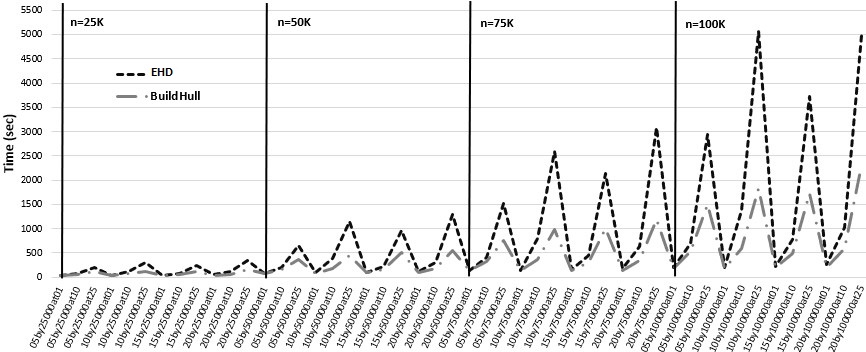
Figure 1: Execution times for all data sets in the MassiveScaleDEAdata sorted by Cardinality$\rightarrow$Dimension$\rightarrow$Density.

The results allow the following conclusions about the two procedures’ running times as evident in Figure 1:

1. BuildHull is faster than EHD in all 48 instances for the data sets in the MassiveScaleDEAdata suite using sequential implementations. The advantage of BuildHull over EHD can be attributed to the additional large LPs solved in Step 4 of the latter.

2. The procedures are closest in time for 05by25000at01 with 39.74 secs. for BuildHull vs 40.70 secs. for EHD, while the biggest difference occurs at 10by100000at25 with 1,817.77 secs. for BuildHull vs 5,051.58 secs. for EHD.

3. For a given dimension and density, running time increases with cardinality.

4. Within each cardinality we can appreciate how time clearly increases with density and how the effect is more severe for Procedure EHD.

5. The closest gaps between the two procedures occur at $d=1\%$.

In the following discussion, computational results are presented and discussed in terms of the effect of density, $d$, cardinality, $n$, and dimension, $m$, using representative values of the parameters.

Density: $d$. The four panels in Figure 2 compare the effect of density, $d$, on the running time performance of the two procedures for the data sets with highest cardinality, $n=$100K, across four dimensions. The four plots depict how the two procedures start at almost the same speed when $d=1\%$ and, as the density increases, BuildHull gains an advantage over EHD ending up more than twice as fast when $d=25$. This relative performance based on density using these massive data sets is representative of what occurs with the rest of the point sets in the MassiveScaleDEAdata suite.

As noticed, the number of LPs solved in Steps 2 and 3 of EHD equals the total number of LPs solved in BuildHull. Also, Step 2 solves $(p-\hat{m})$ LPs of size $p=\sqrt{n}$, while Step 3 solves $(n-p)$ LPs of size less than or equal to $p$, see Table 2. Given that there are only frame elements on the boundary of the production possibility set in the MassiveScaleDEAdata suite and that $\hat{m}=m$ in all its instances, a lower bound on the average LP size in Step 4 is $|{\cal F}|$. When both density and cardinality are small, $|{\cal F}|$ is not much greater than $p$: e.g. $d=1\%,n=25K\Rightarrow|{\cal F}|=250,p=\sqrt{25,000}=158$. However, as $d$ and $n$ increase, the difference between $|{\cal F}|$ and $p$ becomes much greater to the point when $d=25\%,n=100K\Rightarrow|{\cal F}|=25,000,p=316$. This explains the relatively narrow running time differences for the two procedures when density and cardinality are small and the large gap when $|{\cal F}|\gg\sqrt{n}$ which occurs when density is high in large cardinalities portrayed in Figures 1 and 2.

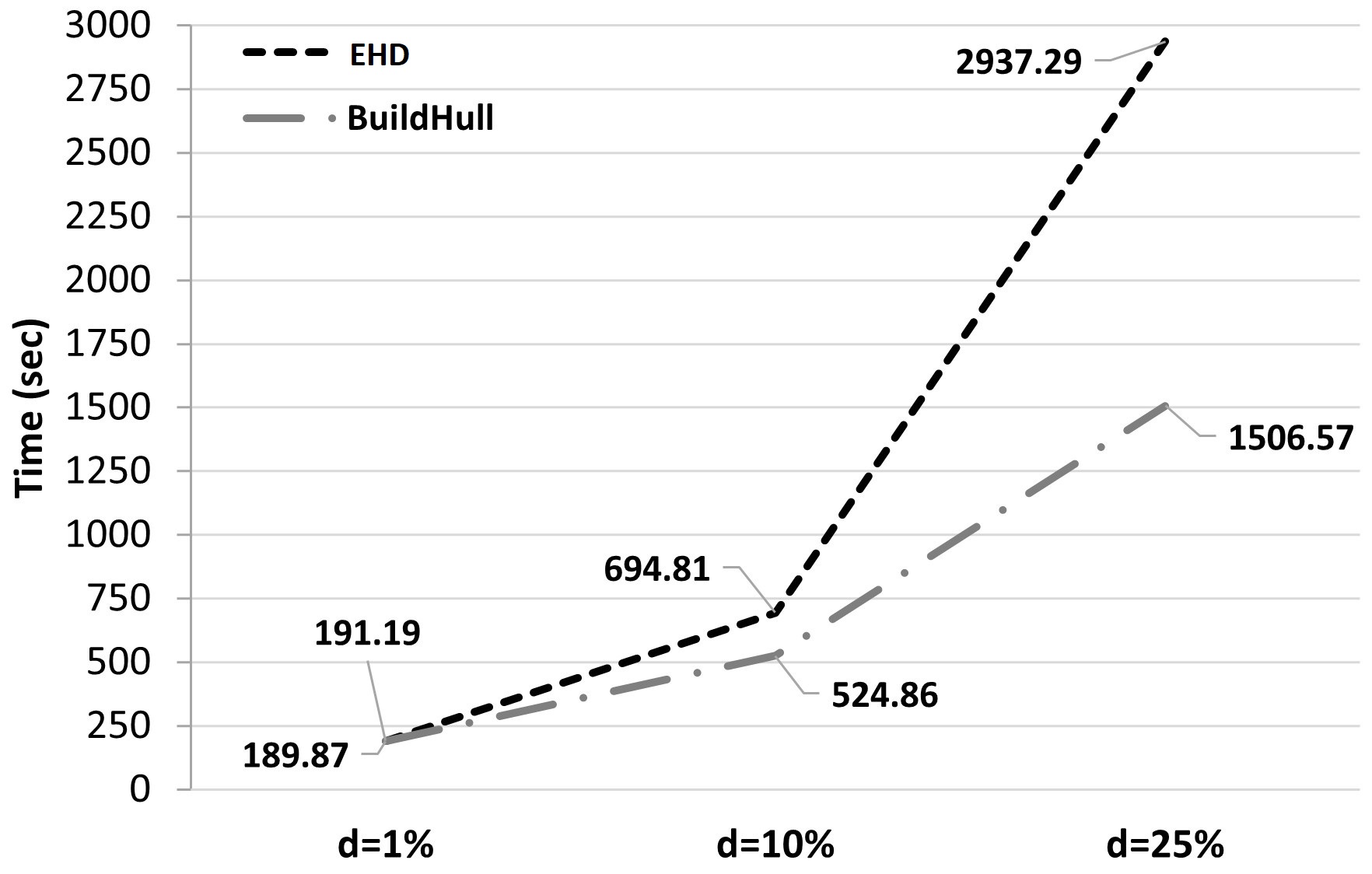
(a) $n=100$K, $m=5$

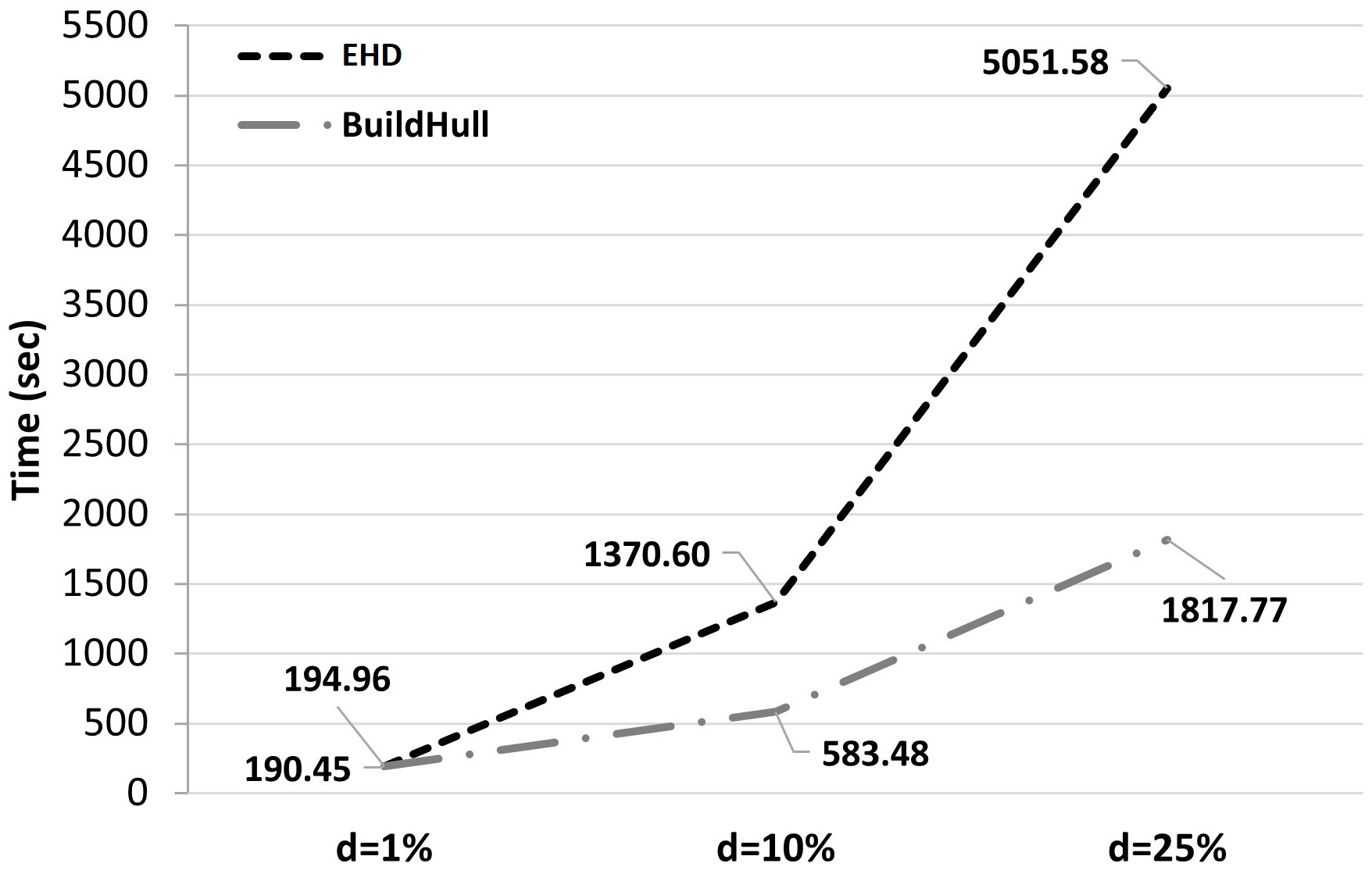
(b) $n=100$K, $m=10$

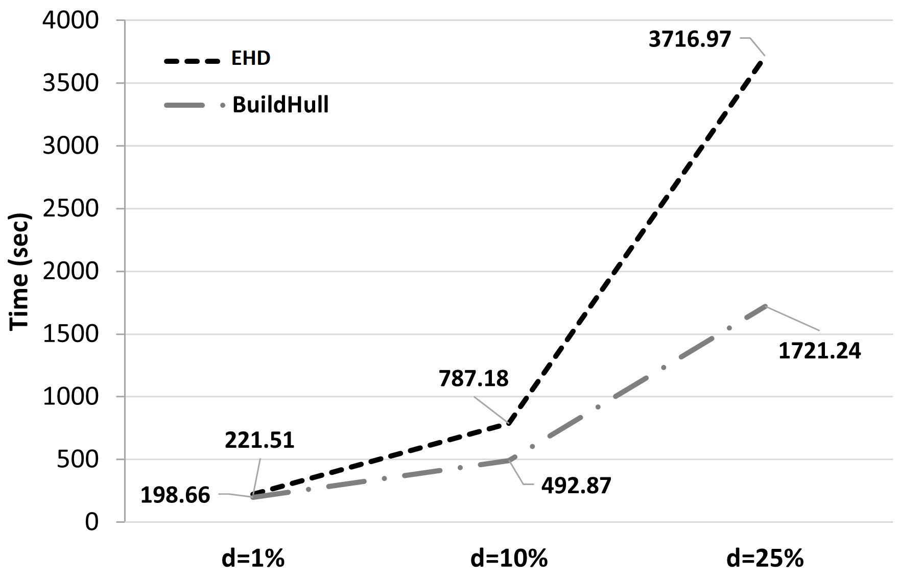
(c) $n=100$K, $m=15$

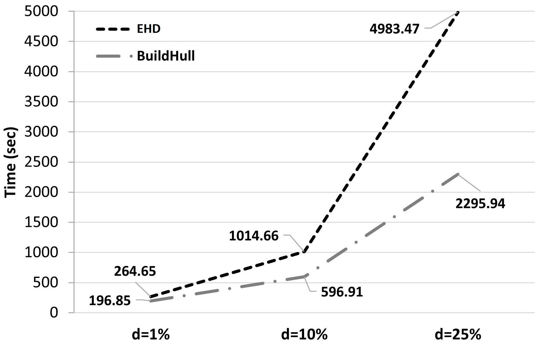
(d) $n=100$K, $m=20$

Figure 2: Impact of density on running time for the data sets in the MassiveScaleDEAdata suite when the cardinality is $n=$100K.

Cardinality: $n$. The four charts in Figure 3 illustrate how cardinality impacts execution time for the data sets with density $d=10\%$ – a value for $d$ typical of what was observed throughout. Similar to the effect of density, the running time performance gaps based on cardinality start small for the lowest cardinality, but widens as its value increases for all four dimensions. For the experiments portrayed in Figure 3, the speedups of BuildHull  over EHD when $n=100$K range from 1.3 to 2.3. This performance gap does not grow uniformly by dimension $m$: the ratio goes from 2.3 when $m=10$ to 1.6 for $m=15$. We will see that data sets with dimension $m=10$ will also be of interest when we study the effects of dimension next. The plots exhibit a familiar, although slight, quadratic behavior previously reported (see, e.g. [9], [8]) for both procedures.

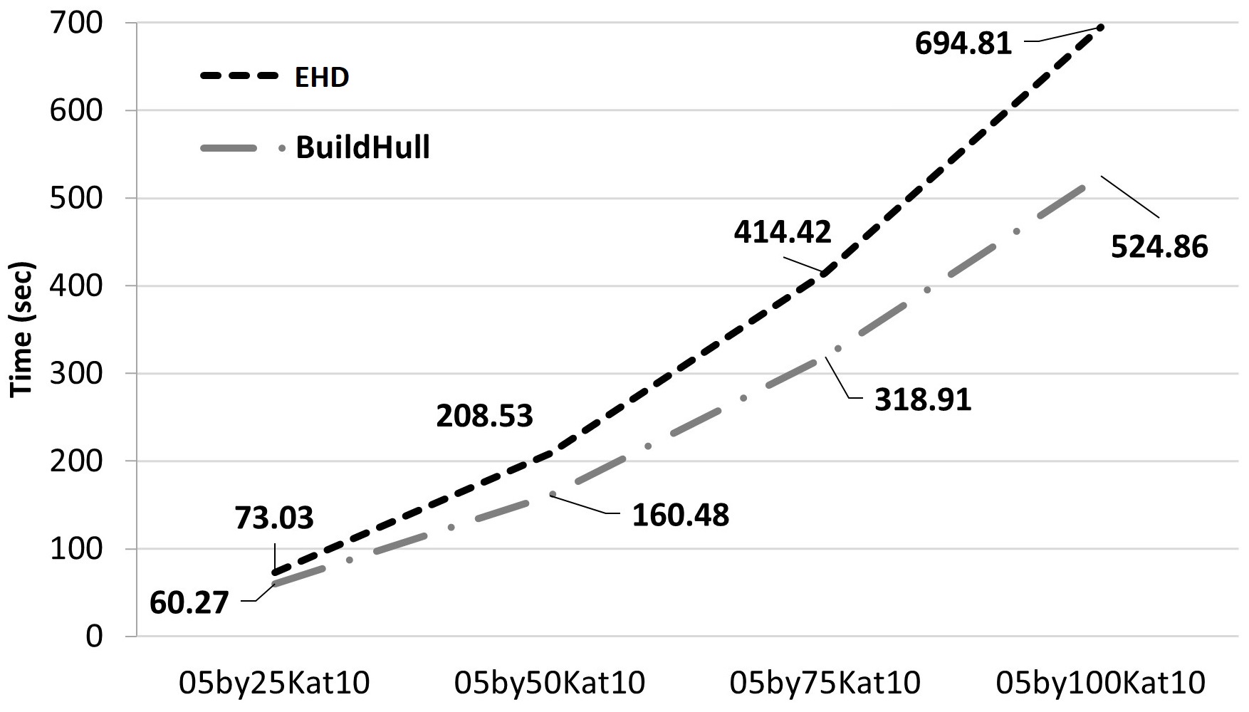
(a) $d=10\%$, $m=5$

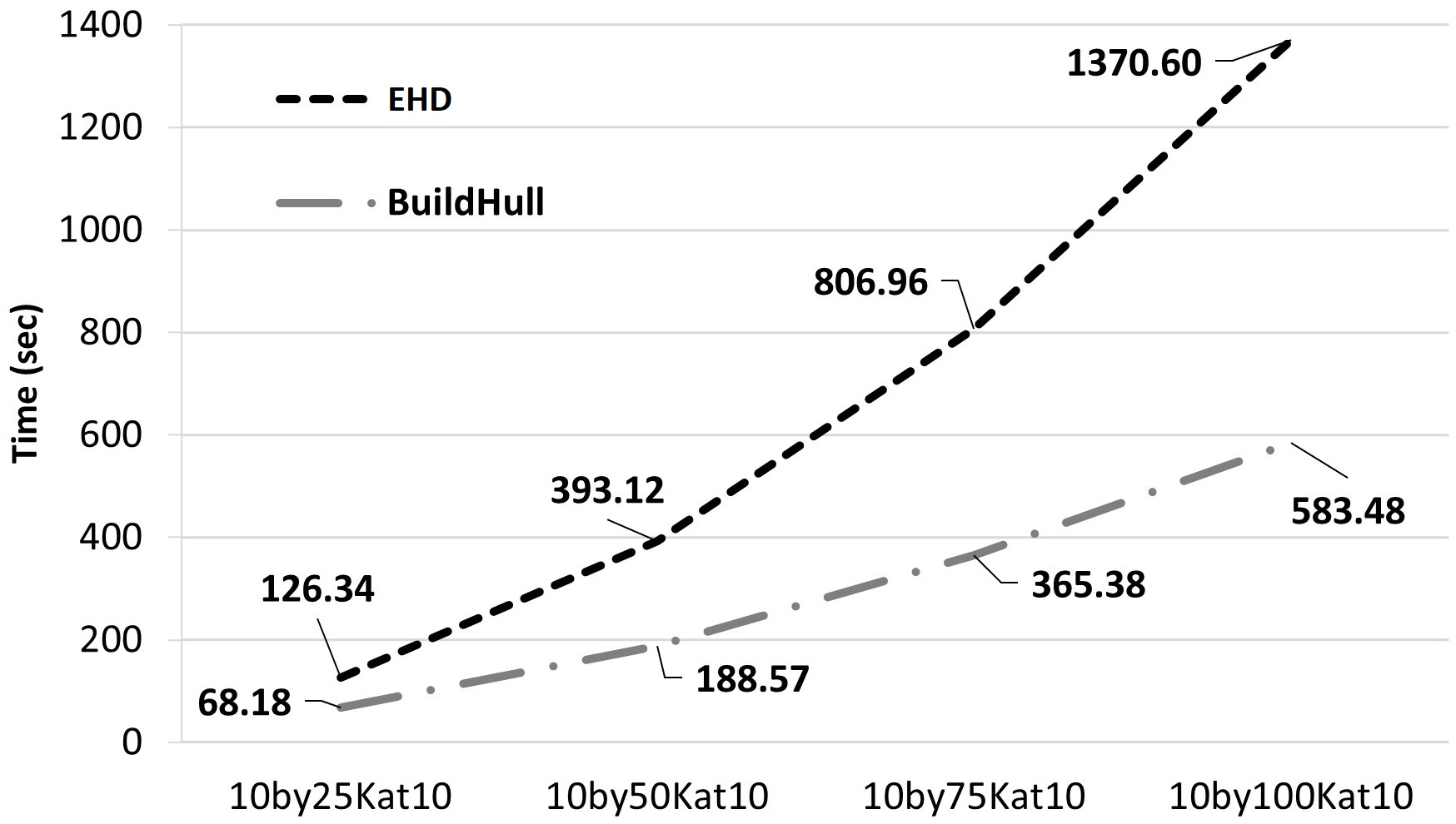
(b) $d=10\%$, $m=10$

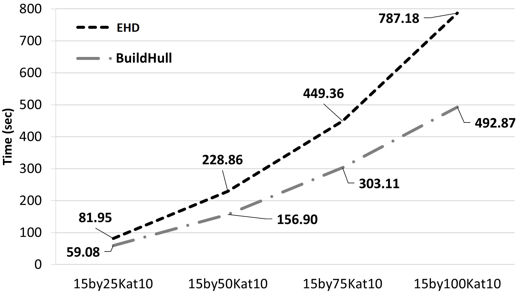
(c) $d=10\%$, $m=15$

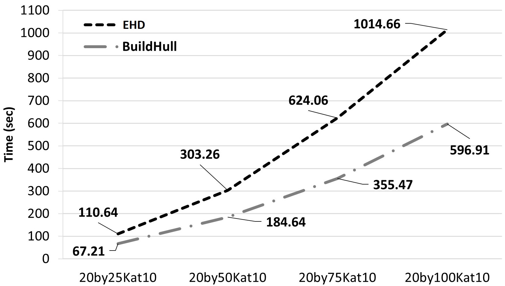
(d) $d=10\%$, $m=20$

Figure 3: Impact of cardinality on running time for the data sets in the MassiveScaleDEAdata suite when the density is $d=10\%$.

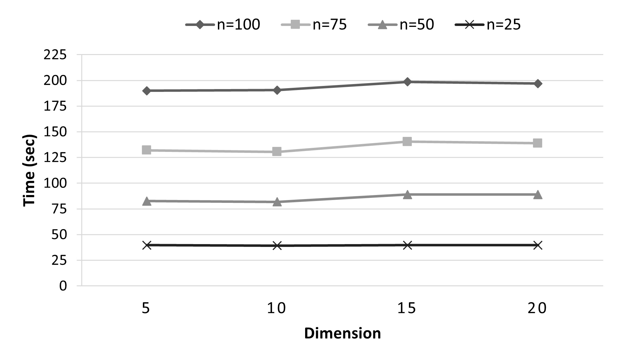
(a) BuildHull, $d=1\%$

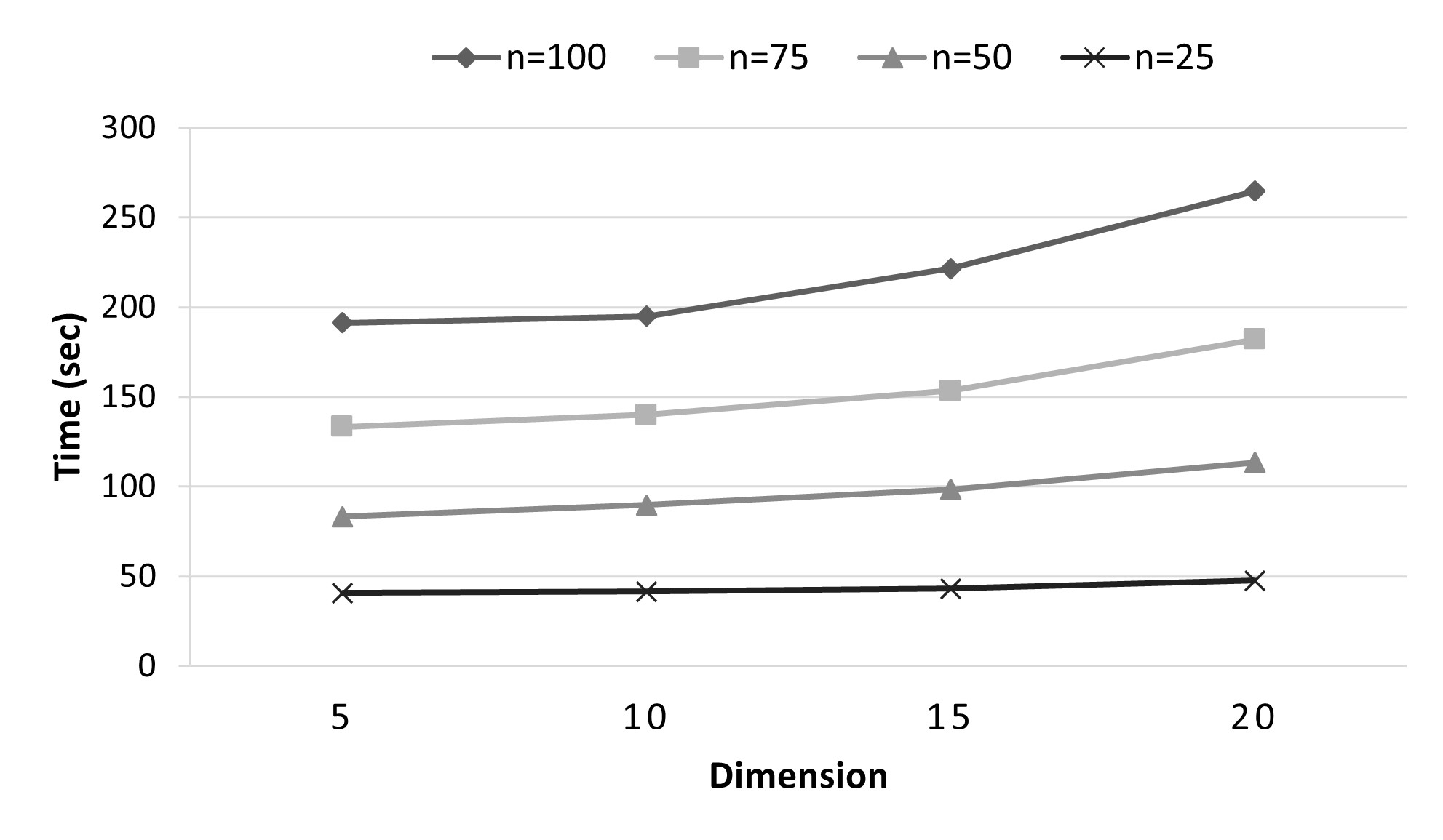
(b) EHD, $d=1\%$

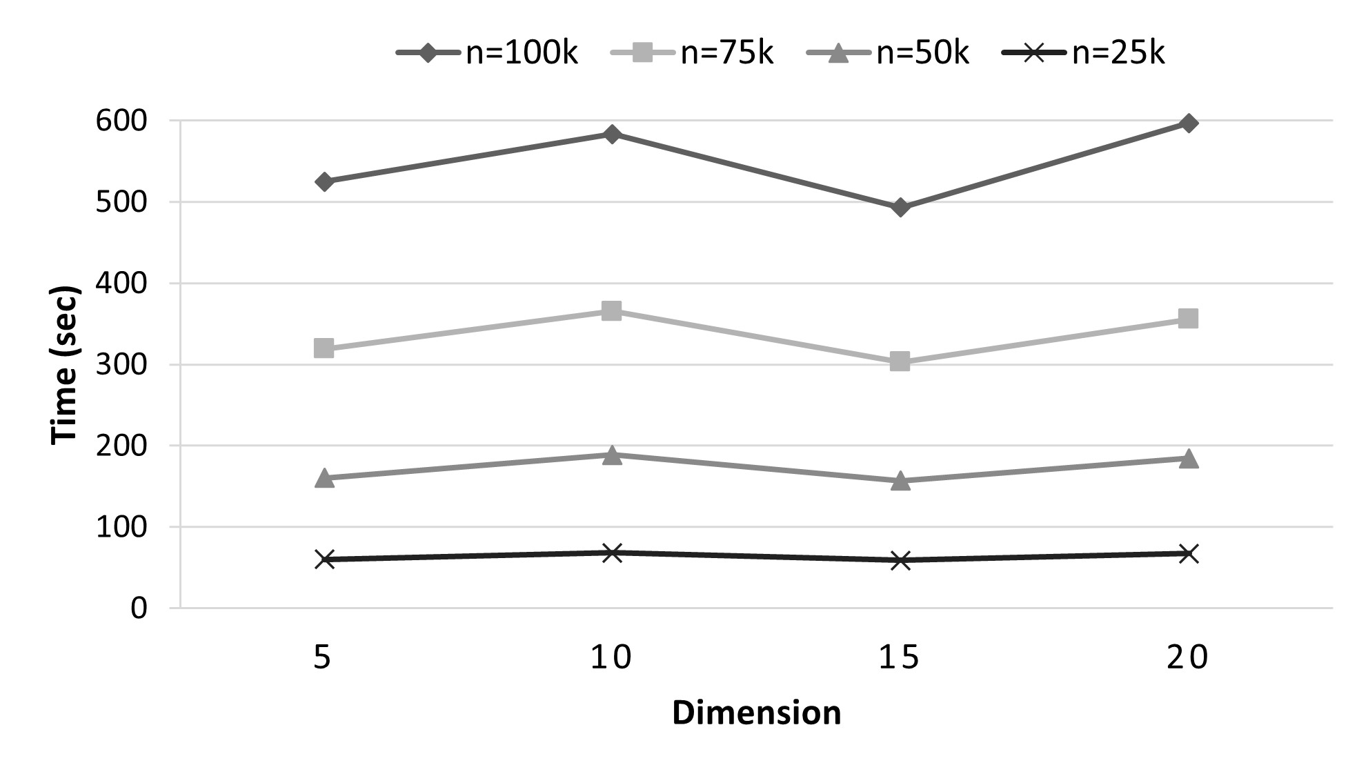
(c) BuildHull, $d=10\%$

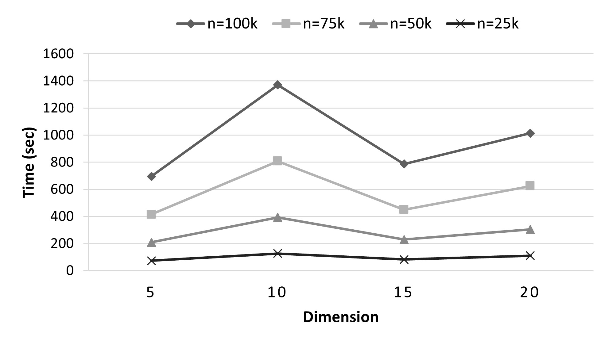
(d) EHD, $d=10\%$

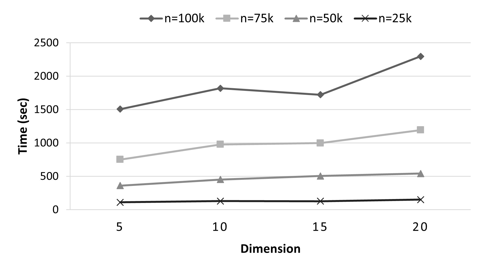
(e) BuildHull, $d=25\%$

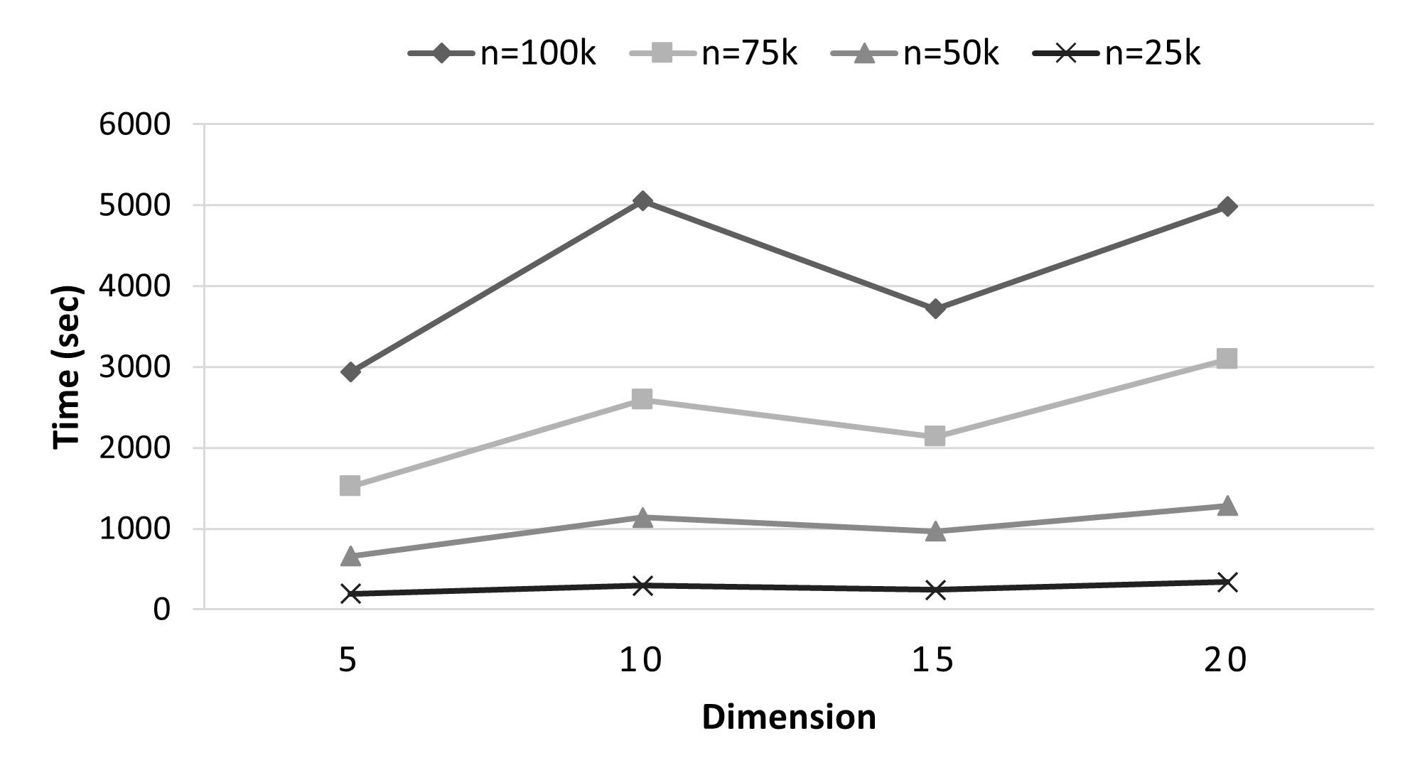
(f) EHD, $d=25\%$

Figure 4: Impact of dimension on running time for data sets in the MassiveScaleDEAdata suite.

Dimension: $m$. The six panels in Figure 4 report on the relation between dimension $m$ and running time for the three densities $d=1\%,d=10\%,d=25\%$ in the MassiveScaleDEAdata suite for both procedures. Each panel superimposes the measurements for the four cardinalities. An unexpected reduction in running time from $m=10$ to $m=15$ for the four cardinalities is clearly visible in the panels (4c) & (4d) and (4e) & (4f) of Figure 4. This effect becomes more obvious as cardinality increases and more evident for EHD. A similar effect was observed in [9] on the same MassiveScaleDEAdata suite. Results from [9] include instances of non-monotonicity, or a milder non-uniform rate of increase, in running time as dimension increases. This occurs for data sets in the suite with $m=10$, e.g. **by25000at25 and **by100000at10 (see appendix in [9]). The fact that the reduction in running time occurs for similar values of $m$ & $d$ in both procedures in the current implementation is evidence that the phenomenon is connected to an intrinsic characteristic of the data sets involved. In particular, for these datasets, the number and size of LPs solved in Step 4 of EHD are greater for $m=10$ than the corresponding ones with $m=15$. For instance, from Table 9, we see that, for data set 10by100000at10, Step 4 of EHD solves 17,125 LPs each with 17,136 variables for an execution time of 1370.6 secs., whereas for the higher dimensional data set, 15by100000at10, 10,097 LPs are solved each with 10,113 variables for an execution time of 787.18 secs. For BuildHull, for these same two datasets, the average LP size is higher (1387.13) for $m=10$ than the one where $m=15$ (804.52), resulting in execution times of 583.48 secs. and 492.87 secs., respectively (see Table 13).

The non-intuitive effect where the increased dimension causes a reduction in execution time in some data sets appears in both the current implementation of BuildHull and the one in 2011 [9]. This suggests that the cause is related to characteristics of the data and how they affect the geometry of the partial hulls generated in the procedures. However, this also suggests that preprocessors are also playing a role. In the case of EHD, the productivity of preprocessors is low for the eight datasets with $m=10$ dimensions, i.e., 10by$-n-$at10 and 10by$-n-$at25; for $n=25K,50K,75K,100K$, see Tables 6-9. Recall that we defined productivity for EHD as the number of interior data points from ${\cal A}$ contained in the partial hull $\mathop{\tt vrs}\limits({\cal A}^{S})$ and identified in Steps 2 & 3. Productivity is a direct measurement of the effectiveness in Procedure EHD of the two preprocessors: dimension sorting and the pre-scoring heuristic. Also, productivity determines the number and size of LPs solved in Step 4 of EHD: the higher the productivity of $\mathop{\tt vrs}\limits({\cal A}^{S})$, the closer the size of the LPs will be to the lower bound of $|{\cal F}|$. For instance, the productivity of 10by100000at10 dataset is almost 100% while for 15by100000at10 is about 92%. The low productivity of the preprocessors for the aforementioned eight data sets explains the peculiar performance portrayed in panels (4(d)) and (4(f)) of Figure 4, as more LPs with larger size will be solved by EHD in these cases.

Notice how BuildHull also feels the impact, though much more attenuated, of less effective preprocessing of these data sets as depicted in panels (4(c)) and (4(e)) of Figure 4. These out-of-the-ordinary data sets prove to be useful, as they provide information about how the preprocessors impact the performance of the procedures.

It is clear from the above analysis that preprocessors have a substantial impact on EHD and, when applied in an equitable manner to BuildHull, also renders the latter faster. Ordering the rest of the points in ascending pre-score value facilitates to slow up the rate of growth of the LPs size in BuildHull. The employed preprocessors work best under low density and high dimensionality. Also, Step 4 in Procedure EHD requires considerable computational effort especially in instances where the cardinality of the frame is much larger than the paramenter $p$. This is verified by the experimentaion on MassiveScaleDEAdata suite when the cardinality of the data set is large and its density is high.

6 Conclusions

Direct sequential (non-parallel) implementations of Procedures EHD from [13] and BuildHull in [9] were compared to obtain comprehensive empirical insights about their performances. The comparisons are based on execution times but also using measurements about the number and size of the LPs solved to explain interesting performance characteristics. The implementations establish a common ground for comparisons by applying the same preprocessors or enhancements when they fit. The two procedures were tested on the publicly available and widely used MassiveScaleDEAdata suite of 48 structured, synthetic, data sets. The empirical results of these sequential implementations reveal that BuildHull is always faster than EHD, as speculated in [14]. The computational time advantage of BuildHull relative to EHD is small for data sets with low density and increases as cardinality and density increase reaching speed ups of almost three times faster than EHD  for the largest data sets. Along with execution times, the total number of LPs solved was tracked and their size is calculated. These metrics were used to explain interesting results such as how running time is reduced as dimension increases with both procedures.

A logical next step is a comparison of parallel implementations of BuildHull and EHD. Procedure EHD is directly parallelizable and this has been done in [13]. The parallelization of BuildHull, although less immediate, will have to focus on more granular aspects of the algorithm such as classifying test points as external or internal to a partial hull. The current work lays the foundation for a more theoretical study of the computational complexity of DEA procedures, something which is lacking in BuildHull and EHD and also in all the other important algorithmic contributions in DEA. Another direction for future research is the hybridization of BuildHull with EHD, by applying the former separately to Steps 2, 3 & 4 of the latter. In addition, the insights obtained here about the role of enhancements and preprocessors can be used to improve or develop variations, or new preprocessors outright.

Finally, contributions to computational DEA apply directly to the frame problem in computational geometry [11]. Computational geometry offers a multitude of opportunities for applications of results from computational DEA in the form of algorithmic adaptations and comparisons along with applications on specialized problems outside of DEA.

Appendix A Appendix

Data Set	LP Size Step 2	LP Size Step 3	LP Size Step 4	# of LPs Step 4	Total # of LPs	Total Time
05by25000at01	159	42	926	920	25915	40.70
05by25000at10	159	151	3304	3298	28293	73.03
05by25000at25	159	159	7247	7241	32236	192.43
10by25000at01	159	81	262	251	25241	41.36
10by25000at10	159	140	4602	4591	29581	126.34
10by25000at25	159	155	8119	8108	33098	296.17
15by25000at01	159	96	503	487	25472	43.06
15by25000at10	159	159	2608	2592	27577	81.95
15by25000at25	159	159	6382	6366	31351	244.25
20by25000at01	159	138	262	241	25221	47.55
20by25000at10	159	159	3045	3024	28004	110.64
20by25000at25	159	159	6683	6662	31642	337.29

Table 6: Results of EHD for cardinality $n=25$K in MassiveScaleDEAdata suite.

Data Set	LP Size Step 2	LP Size Step 3	LP Size Step 4	# of LPs Step 4	Total # of LPs	Total Time
05by50000at01	224	71	1596	1590	51585	83.14
05by50000at10	224	222	6531	6525	56520	208.53
05by50000at25	224	224	14643	14637	64632	660.96
10by50000at01	224	155	502	491	50481	89.68
10by50000at10	224	202	8887	8876	58866	393.12
10by50000at25	224	220	15869	15858	65848	1140.77
15by50000at01	224	167	619	603	50588	98.41
15by50000at10	224	224	5093	5077	55062	228.86
15by50000at25	224	224	12638	12622	62607	967.19
20by50000at01	224	210	506	485	50465	113.48
20by50000at10	224	224	5584	5563	55543	303.26
20by50000at25	224	224	13141	13120	63100	1283.35

Table 7: Results of EHD for cardinality $n=50$K in MassiveScaleDEAdata suite.

Data Set	LP Size Step 2	LP Size Step 3	LP Size Step 4	# of LPs Step 4	Total # of LPs	Total Time
05by75000at01	274	84	2561	2555	77550	133.20
05by75000at10	274	269	10078	10072	85067	414.42
05by75000at25	274	274	22175	22169	97164	1522.59
10by75000at01	274	197	754	743	75733	139.96
10by75000at10	274	247	13001	12990	87980	806.96
10by75000at25	274	272	23988	23977	98967	2592.52
15by75000at01	274	202	827	811	75796	153.39
15by75000at10	274	274	7600	7584	82569	449.36
15by75000at25	274	274	18891	18875	93860	2134.45
20by75000at01	274	263	752	731	75711	181.88
20by75000at10	274	274	8219	8198	83178	624.06
20by75000at25	274	274	19419	19398	94378	3092.35

Table 8: Results of EHD for cardinality $n=75$K in MassiveScaleDEAdata suite.

Data Set	LP Size Step 2	LP Size Step 3	LP Size Step 4	# of LPs Step 4	Total # of LPs	Total Time
05by100000at01	317	88	3477	3471	103466	191.19
05by100000at10	317	315	13636	13630	113625	694.81
05by100000at25	317	317	29519	29513	129508	2937.29
10by100000at01	317	225	1001	990	100980	194.96
10by100000at10	317	296	17136	17125	117115	1370.60
10by100000at25	317	314	32178	32167	132157	5051.58
15by100000at01	317	253	1108	1092	101077	221.51
15by100000at10	317	317	10113	10097	110082	787.18
15by100000at25	317	317	25148	25132	125117	3716.97
20by100000at01	317	308	1005	984	100964	264.65
20by100000at10	317	317	10762	10741	110721	1014.66
20by100000at25	317	317	25830	25809	125789	4983.47

Table 9: Results of EHD for cardinality $n=100$K in MassiveScaleDEAdata suite.

Data Set	Total # of LPs	Average LP Size	Total Time
05by25000at01	24995	45.74	39.74
05by25000at10	24995	424.12	60.27
05by25000at25	24995	1331.31	110.98
10by25000at01	24990	33.51	39.18
10by25000at10	24990	429.01	68.18
10by25000at25	24990	1209.34	129.13
15by25000at01	24985	66.22	39.71
15by25000at10	24985	221.18	59.08
15by25000at25	24985	908.63	127.19
20by25000at01	24980	48.91	39.78
20by25000at10	24980	236.70	67.21
20by25000at25	24980	905.09	151.02

Table 10: Results of BuildHull for cardinality $n=25$K in MassiveScaleDEAdata suite.

Data Set	Total # of LPs	Average LP Size	Total Time
05by50000at01	49995	74.31	82.65
05by50000at10	49995	818.03	160.48
05by50000at25	49995	2638.61	359.40
10by50000at01	49990	45.96	81.79
10by50000at10	49990	734.84	188.57
10by50000at25	49990	2380.06	452.18
15by50000at01	49985	74.92	88.96
15by50000at10	49985	413.03	156.90
15by50000at25	49985	1793.22	503.64
20by50000at01	49980	52.65	89.02
20by50000at10	49980	412.23	184.64
20by50000at25	49980	1753.61	541.08

Table 11: Results of BuildHull for cardinality $n=50$K in MassiveScaleDEAdata suite.

Data Set	Total # of LPs	Average LP Size	Total Time
05by75000at01	74995	114.66	131.94
05by75000at10	74995	1241.59	318.91
05by75000at25	74995	3924.94	750.39
10by75000at01	74990	62.53	130.42
10by75000at10	74990	1073.09	365.38
10by75000at25	74990	3617.11	977.13
15by75000at01	74985	82.95	140.36
15by75000at10	74985	621.01	303.11
15by75000at25	74985	2710.10	997.74
20by75000at01	74980	60.54	138.79
20by75000at10	74980	629.17	355.47
20by75000at25	74980	2598.93	1192.76

Table 12: Results of BuildHull for cardinality $n=75$K in MassiveScaleDEAdata suite.

Data Set	Total # of LPs	Average LP Size	Total Time
05by100000at01	99995	149.74	189.87
05by100000at10	99995	1666.37	524.86
05by100000at25	99995	5228.89	1506.57
10by100000at01	99990	80.25	190.45
10by100000at10	99990	1387.13	583.48
10by100000at25	99990	4676.17	1817.77
15by100000at01	99985	89.91	198.66
15by100000at10	99985	804.52	492.87
15by100000at25	99985	3542.93	1721.24
20by100000at01	99980	64.10	196.85
20by100000at10	99980	821.44	596.91
20by100000at25	99980	3561.68	2295.94

Table 13: Results of BuildHull for cardinality $n=100$K in MassiveScaleDEAdata suite.

References

- [1] I. Ali. Streamlined computation for data envelopment analysis. European Journal of Operational Research, 64:61–7, 1993.
- [2] R.D. Banker, A. Charnes, and W.W. Cooper. Some models for estimating technological and scale inefficiencies in Data Envelopment Analysis. Management Science, 30:1078–1092, 1984.
- [3] R.S. Barr and M.L. Durchholz. Parallel and hierarchical decomposition approaches for solving large scale Data Envelopment Analysis models. Annals of Operations Research, 73:339–372, 1997.
- [4] A. Bessent and W. Bessent. Determining the comparative efficiency of schools through Data Envelopment Analysis. Education Administration Quarterly, 16:57–75, 1980.
- [5] A. Charnes, W.W. Cooper, and E. Rhodes. Measuring the efficiency of decision making units. European Journal of Operational Research, 2:429–444, 1978.
- [6] W.-C. Chen and W.-J. Cho. A procedure for large-scale DEA computations. Computers & Operations Research, 36:1813 – 1824, 2009.
- [7] W.-C. Chen and S.-Y. Lai. Determining radial efficiency with a large data set by solving small-size linear programs. Annals of Operations Research, 250:147–166, 2017.
- [8] J.H. Dulá. A computational study of dea with massive data sets. Computers & Operations Research, 35:1191 – 1203, 2008.
- [9] J.H. Dulá. An algorithm for Data Envelopment Analysis. INFORMS Journal on Computing, 23:284–296, 2011.
- [10] J.H. Dulá and F.J. López. Preprocessing dea. Computers & Operations Research, 36:1204–1220, 2009.
- [11] J.H. Dulá and F.J. López. Competing output-sensitive frame algorithms. Computational Geometry: Theory and Applications, 45:186–197, 2012.
- [12] T. Jie. Parallel processing of the build hull algorithm to address the large-scale dea problem. Annals of Operations Research, 295(1):453–481, 2020.
- [13] D. Khezrimotlagh, J. Zhu, W. Cook, and M. Toloo. Data envelopment analysis and big data. European Journal of Operational Research, 274:1047–1054, 2019.
- [14] Dariush Khezrimotlagh. Parallel processing and large-scale datasets in data envelopment analysis. In Data-Enabled Analytics: DEA for Big Data, pages 159–174. Springer, 2021.
- [15] P.J. Korhonen and P.-A. Siitari. Using lexicographic parametric programming for identifying efficient units in dea. Computers & Operations Research, 34(7):2177–2190, 2007.
- [16] P.J. Korhonen and P.-A. Siitari. A dimensional decomposition approach to identifying efficient units in large-scale dea models. Computers & Operations Research, 36(1):234–244, 2009.
- [17] T. Sueyoshi. A special algorithm for an additive model in data envelopment analysis. Journal of the Operational Research Society, 41(3):249–257, 1990.
- [18] T. Sueyoshi and Y.L. Chang. Efficient algorithm for additive and multiplicative models in Data Envelopment Analysis. Operations Research Letters, 8:205–213, 1989.