Score matching for bridges without time-reversals
Abstract
We propose a new algorithm for learning a bridged diffusion process using score-matching methods. Our method relies on reversing the dynamics of the forward process and using this to learn a score function, which, via Doob’s -transform, gives us a bridged diffusion process; that is, a process conditioned on an endpoint. In contrast to prior methods, ours learns the score term , for given directly, completely avoiding the need for first learning a time reversal. We compare the performance of our algorithm with existing methods and see that it outperforms using the (learned) time-reversals to learn the score term. The code can be found at https://github.com/libbylbaker/forward_bridge.
1 Introduction
Given a diffusion process, we consider the problem of conditioning its endpoint to take a specific value or distribution. In general it can be shown by Doob’s -transform that a diffusion process conditioned on a point at time can also be written as a stochastic differential equation Equation 2, which has an extra drift term containing , where is the transition density of the stochastic differential equation. The problem is, this term is general intractable. Finding alternative methods to sample from the bridge process has received considerable attention in the past [Delyon and Hu, 2006, Papaspiliopoulos and Roberts, 2012, Bladt and Sørensen, 2014, Schauer et al., 2017, Heng et al., 2022]. Diffusion processes have a multitude of applications across numerous areas, where observations need to be included, leading to bridge processes (see Papaspiliopoulos and Roberts [2012] for some examples). Recently, bridges have also been used in generative modelling via time reversals, as well as for diffusion bridges. These usually are bridges between two distributions and involve time-reversals of a linear SDE. Singhal et al. [2024] also consider using non-linear SDEs for this purpose and so look at the problem of finding time-reversed bridges of a given SDE. Within shape analysis bridges are applied, for example, to medical imaging, in order to model how the shapes of organs change in the face of disease [Arnaudon et al., 2017], or in evolutionary biology to model how shapes of organisms change over time [Baker et al., 2024].
Contributions
We propose a new algorithm to learn bridge diffusion processes by learning the score term occurring in the conditioned process. We learn this term by combining the score matching methods proposed in Heng et al. [2022], with adjoint diffusions [Milstein et al., 2004]. Importantly, these adjoint diffusions are not time-reversed, rather a reversal of dynamics, meaning they can be simulated directly. This differs from Heng et al. [2022], where in order to learn the score term, they first learn the time-reversed diffusion and then train a second time using the learnt time-reversed diffusions, which introduces a higher error. We compare our method with other existing methods.
2 Background
We are interested in conditioning an SDE to take a certain value at its end time. The conditioned process can again be written as a stochastic differential equation via Doob’s -transform which we describe in Section 2.1. However, this SDE has an intractable term, the score term . In Section 2.2 we discuss the reversal (but not the time-reversal) of the SDE which, up to a correction term , has the transition density when started in at time . In the proposed method, we will use the adjoint processes to directly learn the term , used for forward bridges. Score learning provides a method for learning a similar term and is discussed in Section 2.3.
2.1 Doob’s -transform
Consider a stochastic differential equation defined as
| (1) |
where and is a -dimensional Wiener process. We assume that satisfies a global Lipschitz condition so that Equation 1 has a Markov solution (see Schilling and Partzsch [2014, Theorem 21.23] for details). Then has a transition density , satisfying
It is well known (see e.g. Särkkä and Solin [2019, Chapter 7.5]) that conditioned such that for a fixed , satisfies another stochastic differential equation
| (2) |
with and where is the gradient with respect to the argument . However, the transition density, or rather the score is typically intractable.
2.2 Adjoint processes with reversed dynamics
Here we define the adjoint process of the unconditioned process which receives its name from its relation to the adjoint operator of the infinitesimal generator of seen as Markov process. Intuitively, the adjoint process has the reversed dynamics of the unconditioned process, for example, the adjoint of a Brownian motion with drift , i.e. , is a Brownian motion with drift . In this sense, it is a reversal, but not a time-reversal as in Haussmann and Pardoux [1986]. The theory presented in this section is based on Milstein et al. [2004], Bayer and Schoenmakers [2013] and is also developed in [Van der Meulen and Schauer, 2020, Section 11]. The significance of the adjoint process is that for fixed , we can use it to access and therefore the score . To compare, let be fixed and be a real-valued functional. Then
| (3) |
Here, is a weight process relating to accounting for the fact that adjoint dynamics in general are not Markovian necessitating a Feynman-Kac representation. The right hand side relation of Equation 3 will be integral in our proposed method.
For fixed the adjoint process is defined as follows:
| (4a) | ||||
| (4b) | ||||
The functions are defined in terms of derivatives and second derivatives of from the SDE of with :
| (5a) | |||
| (5b) | |||
| (5c) | |||
From now on, we denote and , but the following also holds for .
Crucially, these quantities can be computed explicitly, either by hand or using automatic differentiation, and therefore we can sample from the adjoint process using, for example, the Euler-Maruyama scheme. Moreover, following [Bayer and Schoenmakers, 2013, Theorem 3.3], we can introduce more time points. For a time grid , and setting it holds
| (6) |
In particular, we can now represent the score as the gradient of the log density , where is the marginal distribution of weighted by , by
| (7) |
2.3 Score matching bridge sampling
In score matching bridge sampling as we consider it, the task is to learn a neural approximation to the score . In our case, samples from weighted with can be used in training, as they represent the unnormalised density . This precisely mimics the use of samples of the noising process in generative diffusion models with in the role of the noising process.
To wit, vanilla score matching as introduced in Hyvärinen [2005] takes the form
| (8) |
Note in particular that knowledge of the transition density is not required. However, in general, computing the divergence term is expensive. To avoid computing the divergence term when learning we instead use a similar loss objective to that proposed in Vincent [2011]
| (9) |
In and of itself, this optimisation problem is still intractable, however, for processes where for some , Ho et al. [2020] show that Equation 9 can be formulated as minimising an alternative loss function
| (10) |
For processes where the transition densities are not known, Heng et al. [2022] instead suggest using the loss objective
| (11) |
Then for small time steps, the transition density can be estimated, for example, using the Euler-Maruyama scheme.
3 Related work
In this section, we survey the existing methods for computing bridge processes. We concentrate specifically on methods that can be applied to any diffusion process to find the forward bridge. For this reason, we deem usual score matching methods as out of scope, since the main motivation of these methods is to find a time-reversal of a specific diffusion, usually an Ornstein-Uhlenbeck.
3.1 Score matching methods
Most related to our work is the method of Heng et al. [2022]. We use a similar loss function, however we take the expectation over (directly simulated) adjoint processes, enabling us to directly learn a forward in time bridge process. One key difference to the time-reversed bridge process is that the forward processes are dependent on the end point but independent of the start point, whereas the time-reversals are dependent on the start point and independent of the end point. This is because the proposed method learns the term with fixed, whereas the method in Heng et al. [2022] learns with fixed. Iterating over the method twice enables one to learn but we show that for learning a forward in time bridge, our proposed method is advantageous in that we only need train once, thereby reducing the approximation error.
Recently, Singhal et al. [2024] consider using non-linear SDEs instead of linear ones within generative modelling, meaning the transition densities for the SDE are also unknown. However, instead of using Euler-Maruyama approximations for the transition kernels as in Heng et al. [2022], they consider other higher-order approximations. Unlike ours, their work only considers time-reversals in the context of generative modelling and not forward bridges.
3.2 MCMC methods
One method of sampling from the bridge processes is to sample from a second approximate bridge, where the ratio between the true bridge and the approximate bridge is known. For an unconditional process as in Equation 1, the approximate bridges have form
| (12) |
where different authors have considered different options for the function . In Pedersen [1995] , that is, the samples are taken from the original unconditioned process. Delyon and Hu [2006] instead take the Brownian bridge drift term. More recently, Schauer et al. [2017] set to be the term arising from conditioning an auxiliary process with a known transition density. With all approximations, one can derive a ratio between the path probability of the true bridge and the bridge approximation and can therefore use Markov Chain Monte Carlo methods to sample from the true distribution.
4 Method
This section presents our neural-network based algorithm to find the score function that will be used to simulate the bridge process. In Section 4.1 we derive the main loss function for learning the score function and show it minimises the Kullback-Leibler divergence between the conditioned path and the path measure induced by the learnt conditioned process. In Section 4.2 we provide details on how we minimise the loss function. In Section 4.3 we show that we can also train for different values of , and we can also condition on following a distribution, instead of being a fixed point. Proofs can be found in Section A.1.
4.1 A loss function
In order to sample the bridged stochastic differential equation, we learn the score term for fixed . Note that although similar, this is different from the term that is learnt for time-reversed processes, as in score-matching for diffusion samplers. Indeed, score-matching methods rely on the SDE having as a transition density, and therefore by sampling from the process , we are sampling from the distribution of the process at time , directly leading to the transition density. This is not true for . Our proposal is instead to sample from the adjoint stochastic process, where we can recover the transitions .
Given a function , we define the SDE with path distribution as
| (13) |
In what follows, let be a function, such that as , for the dirac delta function. For fixed with (as defined in Equations 4a and 4b) and we introduce the functional
| (14) |
By minimising this, we are minimising the Kullback-Leibler divergence between the path probability of with initial value in Equation 2, and the path probability of paths as in Equation 13, with the same initial value :
Theorem 4.1.
Let be a diffusion process as defined in Equation 1 and suppose further that are and that admits transition densities. Let be the conditioned diffusion satisfying Equation 2. Let be the path probability of and the path probability of in Equation 13 for a function . Then
where the infimum is taken over functions .
Proof.
In order to prove this, we combine two tricks. The first is to use the adjoint stochastic differential equation, studied in Bayer and Schoenmakers [2013], to write the expectations as integrals over the transition densities . The second, as proposed in Heng et al. [2022], uses the Chapman-Kolmogorov equation to split the integration into smaller, approximable parts. A full proof is given in Section A.1.1. ∎
We have shown that finding that minimises the loss function in Equation 14, also minimises Kullback-Leibler divergence between the conditioned path probability space (which we would like to access) and the path space . The difference is that it is possible to approximate . For example, we can take small, and for small we can approximate .
4.2 Optimising the loss function
To solve the optimisation problem, we let be parameterised by a neural network. We simulate batches of trajectories of the adjoint process using the Euler-Maruyama algorithm. We then approximate the loss function as
| (15) |
where and is a batch of simulations of the SDE started at the value on which we are conditioning. We take to be an Euler-Maruyama step
| (16) |
approximating the score term as proposed in Heng et al. [2022]. In practice, we take , which is equivalent to allowing the forward conditioned process to start from anywhere. Note that the learnt quantity is not dependent on . The exact algorithm as described above is shown in Algorithm 1.
4.3 Training on multiple end points
We can extend to training on multiple end points in two ways. The first is where the end point is not fixed, rather sampled from some distribution . The second, is where we learn fixed for multiple values at once; that is for fixed and variable , we learn . Both of these are straightforward extensions to our method.
Distributions of endpoints
To condition on a distribution instead of a fixed endpoint , we instead integrate over the loss function for different values of . In practice, all that changes is instead of simulating trajectories starting from the same value , we now also sample the start value . Letting , the loss in Equation 15 function becomes
| (17) |
Multiple fixed endpoints
For varied , we integrate the loss function in Equation 14 over and take the loss over functions . Then for the set of ’s that we are interested in, we take a batch of uniformly distributed . In practice, the loss function that we optimise changes from Equation 15 to
| (18) |
where we have used , to mean the adjoint process started from at time .
5 Experiments
In general, we compare only to methods that consider the problem where we are given a path distribution that we condition on given boundary conditions. This is different to the setup of generative modelling or denoising diffusion bridge models, where the boundary points or boundary distributions are given and a bridge is found between them, since in the generative modelling setup, any path distribution can be used for bridging. In this case, a natural choice is then a linear path, where transition densities are known explicitly.
5.1 Ornstein–Uhlenbeck
As a first set of experiments, we consider an Ornstein-Uhlenbeck process. For this process, the score is known and therefore we can compare exactly between the learnt and true score.
To evaluate our method, we compare to Heng et al. [2022], since they also learn the score term . We also compare to their learning of the term , which is used for the time-reversed bridges and must be learnt as a first step in computing the forward bridges.
In the experiments, we take the Ornstein-Uhlenbeck process defined as
| (19) |
Then the adjoint and correction processes are given by
| (20a) | ||||
| (20b) | ||||
and the score function for is given by
| (21) |
where the functions are the mean and variance defined as
| (22) |
In our first experiment we train on fixed end points of that fall between and , as discussed in Section 4.3. The starting values are sampled uniformly from and we train on iterations each with sample paths. We plot the absolute error of the score in Figure 1. We see the absolute error is reasonably low with slightly higher errors towards and where the score has relatively higher values.
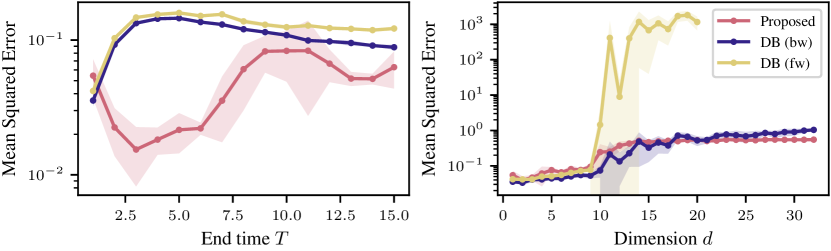
To compare to the method of Heng et al. [2022], we use the code from the authors111Via https://github.com/jeremyhengjm/DiffusionBridge.. In Figure 2, we plot the squared error averaged over time points from to for various dimensions with , and various starting values , with . We compare this to the forward and time-reversed (or backwards) diffusion bridges from Heng et al. [2022]. The time-reversed, DB (bw), learns a different term to ours, , and the forward, DB (fw) uses the time-reversed to learn the same term as our proposed method. For all methods we train on 100 iterations of 1000 samples. We train each one with five different random seeds and plot the average mean square error and the standard deviation between the different trainings.
We see that the Diffusion Bridge (forward) method has a similar error to the proposed method, whereas the reverse method has a much higher error and seems to break down for larger dimensions.

5.2 Brownian motion on distributed endpoints
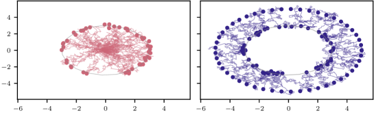
To demonstrate the method in conditioning on a distribution, we next condition a Brownian motion on hitting a circle. That is, we take the SDE , and we sample the end points uniformly from a circle of radius . In Figure 3 (left), we plot trajectories each starting from the origin, and conditioned to hit the circle at time . In Figure 3 (right) we plot trajectories, this time starting from evenly sampled initial values on a circle of radius . Note that both figures use the same trained score function. We only need to train once, since the training is independent of the initial value , and only depends on the final value or distribution that we are conditioning on.
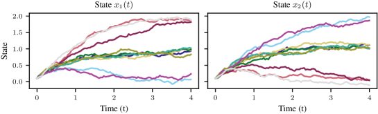
5.3 Cell model
We next consider the cell differentiation and development model from Wang et al. [2011]. This model is also considered in Heng et al. [2022]. The stochastic differential equation is given by
| (23) | |||
| (24) |
and describes the process of cell differentiation into three specific cell types. In Figure 4 we plot some trajectories for the unconditioned process for illustration purposes.
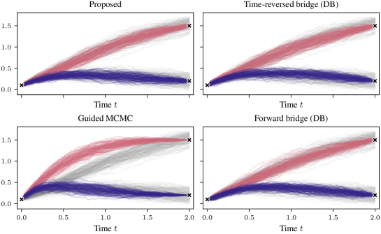
In our experiment we compare to the time-reversed bridge and the forward bridge of Heng et al. [2022] (again using the code from the authors 222https://github.com/jeremyhengjm/DiffusionBridge) and the guided bridge method from Schauer et al. [2017]. The true bridge is unknown, so instead we compare against trajectories from the unconditioned process that end near the boundary values. In Figure 5, we plot in grey trajectories from the unconditioned process satisfying at time . We then plot trajectories starting at , conditioned on at time , via the proposed method, the forward bridge (DB) of Heng et al. [2022] and with MCMC using guided proposals as suggested in Schauer et al. [2017].
For the time-reversed bridge, the trajectories are simulated starting at the end point , and run backwards in time, being conditioned to hit the point . We then use trajectories from the time-reversed SDE to train the forward bridge as stated in Heng et al. [2022, Section 2.3]. For the proposed method, the time-reversed bridge (DB) and the forward bridge (DB), we train on trajectories in total with batch sizes of . We use the same network structure for both the proposed method and the time-reversal with the same number of layers, however the proposed method is written in Jax [Bradbury et al., 2018], whereas the other uses Pytorch [Paszke et al., 2019].
For the guided method we use the code from the authors 333Codebase at https://github.com/mschauer/Bridge.jl from file project/partialbridge_fitzhugh.jl. We first simulate trajectories, without saving, and from then save every trajectory, with .
We see in Figure 5 that the proposed method, the time-reversed bridge and the forward bridge produce similar trajectories that seem to follow the correct data distribution. However, note that the proposed method needed only be trained once using trajectories from the adjoint process, whereas the forward bridge was trained on the time-reversed trajectories thereby needing two training.
6 Advantages, disadvantages and concluding remarks
We have shown that we can use adjoint processes to learn the score term for given . This is applied to simulate forward trajectories of bridged diffusion processes. When compared to the method in Heng et al. [2022] for simulating forward in time bridges, we have demonstrated in our experiments that using the adjoints can lead to an estimation with lower error and negates the need for a second training when the forward in time bridges. Learning the score also seems to perform well compared to using MCMC methods to sample trajectories. However, we note that MCMC methods will likely perform better when conditioning on extremely unlikely events, that will not be seen in the generated data.
7 Acknowledgements
The work presented in this article was done at the Center for Computational Evolutionary Morphometry and is partially supported by the Novo Nordisk Foundation grant NNF18OC0052000, by the Chalmers AI Research Centre (CHAIR) (“Stochastic Continuous-Depth Neural Network”) as well as a research grant (VIL40582) from VILLUM FONDEN and UCPH Data+ Strategy 2023 funds for interdisciplinary research.
References
- Delyon and Hu [2006] Bernard Delyon and Ying Hu. Simulation of conditioned diffusion and application to parameter estimation. Stochastic Processes and their Applications, 116(11):1660–1675, November 2006. ISSN 03044149.
- Papaspiliopoulos and Roberts [2012] Omiros Papaspiliopoulos and Gareth Roberts. Importance sampling techniques for estimation of diffusion models. Statistical methods for stochastic differential equations, 124:311–340, 2012.
- Bladt and Sørensen [2014] Mogens Bladt and Michael Sørensen. Simple simulation of diffusion bridges with application to likelihood inference for diffusions. Bernoulli, pages 645–675, 2014.
- Schauer et al. [2017] Moritz Schauer, Frank Van Der Meulen, and Harry Van Zanten. Guided proposals for simulating multi-dimensional diffusion bridges. Bernoulli, 23(4A), November 2017. ISSN 1350-7265. doi: 10.3150/16-BEJ833.
- Heng et al. [2022] Jeremy Heng, Valentin De Bortoli, Arnaud Doucet, and James Thornton. Simulating diffusion bridges with score matching, October 2022. arXiv:2111.07243.
- Singhal et al. [2024] Raghav Singhal, Mark Goldstein, and Rajesh Ranganath. What’s the score? Automated denoising score matching for nonlinear diffusions. In Forty-first International Conference on Machine Learning, 2024.
- Arnaudon et al. [2017] Alexis Arnaudon, Darryl D Holm, Akshay Pai, and Stefan Sommer. A stochastic large deformation model for computational anatomy. In Information Processing in Medical Imaging: 25th International Conference, IPMI 2017, Boone, NC, USA, June 25-30, 2017, Proceedings 25, pages 571–582. Springer, 2017.
- Baker et al. [2024] Elizabeth Louise Baker, Gefan Yang, Michael L. Severinsen, Christy Anna Hipsley, and Stefan Sommer. Conditioning non-linear and infinite-dimensional diffusion processes, February 2024. arXiv:2402.01434.
- Milstein et al. [2004] Grigori N. Milstein, John G.M. Schoenmakers, and Vladimir Spokoiny. Transition density estimation for stochastic differential equations via forward-reverse representations. Bernoulli, 10(2), April 2004. ISSN 1350-7265. doi: 10.3150/bj/1082380220.
- Schilling and Partzsch [2014] René L. Schilling and Lothar Partzsch. Brownian motion: an introduction to stochastic processes. De Gruyter textbook. de Gruyter, Berlin ; Boston, second edition edition, 2014. ISBN 978-3-11-030729-0.
- Särkkä and Solin [2019] Simo Särkkä and Arno Solin. Applied Stochastic Differential Equations. Cambridge University Press, 1 edition, April 2019. ISBN 978-1-108-18673-5 978-1-316-51008-7 978-1-316-64946-6. doi: 10.1017/9781108186735.
- Haussmann and Pardoux [1986] Ulrich G Haussmann and Etienne Pardoux. Time reversal of diffusions. The Annals of Probability, pages 1188–1205, 1986.
- Bayer and Schoenmakers [2013] Christian Bayer and John Schoenmakers. Simulation of forward-reverse stochastic representation for conditional diffusions. The Annals of Applied Probability, 24, June 2013. doi: 10.1214/13-AAP969.
- Van der Meulen and Schauer [2020] Frank Van der Meulen and Moritz Schauer. Automatic backward filtering forward guiding for Markov processes and graphical models, 2020. 2010.03509v2.
- Hyvärinen [2005] Aapo Hyvärinen. Estimation of non-normalized statistical models by score matching. Journal of Machine Learning Research, 6(24):695–709, 2005.
- Vincent [2011] Pascal Vincent. A connection between score matching and denoising autoencoders. Neural computation, 23(7):1661–1674, 2011.
- Ho et al. [2020] Jonathan Ho, Ajay Jain, and Pieter Abbeel. Denoising diffusion probabilistic models. Advances in neural information processing systems, 33:6840–6851, 2020.
- Pedersen [1995] Asger Roer Pedersen. Consistency and asymptotic normality of an approximate maximum likelihood estimator for discretely observed diffusion processes. Bernoulli, pages 257–279, 1995.
- Wang et al. [2011] Jin Wang, Kun Zhang, Li Xu, and Erkang Wang. Quantifying the Waddington landscape and biological paths for development and differentiation. Proceedings of the National Academy of Sciences, 108(20):8257–8262, 2011.
- Bradbury et al. [2018] James Bradbury, Roy Frostig, Peter Hawkins, Matthew James Johnson, Chris Leary, Dougal Maclaurin, George Necula, Adam Paszke, Jake VanderPlas, Skye Wanderman-Milne, and Qiao Zhang. JAX: composable transformations of Python+NumPy programs, 2018. URL http://github.com/google/jax.
- Paszke et al. [2019] Adam Paszke, Sam Gross, Francisco Massa, Adam Lerer, James Bradbury, Gregory Chanan, Trevor Killeen, Zeming Lin, Natalia Gimelshein, Luca Antiga, et al. Pytorch: An imperative style, high-performance deep learning library. Advances in neural information processing systems, 32, 2019.
Appendix A Appendix
A.1 Proofs
A.1.1 Proof of Theorem 4.1
Theorem.
Let be the path probability of the conditioned diffusion in Equation 2, and the path probability of in Equation 13 for a function . Then
where the infimum is taken over functions .
Proof.
The Kullback-Leibler divergence is defined by
| (25) |
By Girsanov’s theorem, [Schilling and Partzsch, 2014, Theorem 19.9]
| (26) |
Since the expectation of a martingale is equal to , we see that
| (27a) | ||||
| (27b) | ||||
| (27c) | ||||
By [Bayer and Schoenmakers, 2013, Theorem 3.7], this is equal to
| (28) |
We next focus on the contents of the expectation. Writing out in full as , using in place of and expanding the square, we see
| (29a) | ||||
| (29b) | ||||
| (29c) | ||||
| (29d) | ||||
We focus on the third term, Equation 29d. Multiplying this out further and using [Bayer and Schoenmakers, 2013, Theorem 3.6], we see that
| (30a) | ||||
| (30b) | ||||
| (30c) | ||||
Using Chapman-Kolmogorov it holds that for any ,
| (31) |
and so, using the properties of the differential of the logarithm it holds
| (32) |
Putting this back into Equation 30c and using Bayer and Schoenmakers [2013, Theorem 3.6] we get,
| (33a) | ||||
| (33b) | ||||
From this we see that Equation 29d becomes
| (34) |
∎