Persistence-based Modes Inference

Abstract

We consider the estimation of multiple modes of a (multivariate) density. We start by proposing an estimator of the $H_{0}$ persistence diagram. We then derive from it a procedure to estimate the number of modes, their locations and the associated local maxima. For large classes of piecewise-continuous functions, we show that these estimators achieve nearly minimax rates. These classes involve geometric control over the discontinuities set and differ from commonly considered function classes in mode(s) inference. Although the global regularity assumptions are stronger, we do not suppose regularity (or even continuity) in any neighborhood of the modes.

Introduction

Modes are simple measures to describe central tendencies of a density and one of the most used tool to process data. Modes inference finds applications in wide varieties of statistical task, as highlighted in the recent survey by Chacón (2020). Among them, modal approach in clustering has gathered significant attention (Fukunaga and Hostetler, 1975; Cheng, 1995; Comaniciu and Meer, 2002; Li et al., 2007; Chazal et al., 2011; Chacón, 2012; Jiang and Kpotufe, 2017).

The problem of mode(s) inference dates back to Parzen (1962) and has received considerable attention since. The question of consistency and convergence rates of estimators has occupied a central place. The bulk of work on this question is large but has mainly been concentrated on single mode estimation. For this problem, the popular approach is to consider an estimator of the form $\hat{x}=\arg\max_{x\in[0,1]^{d}}\hat{f}(x)$ with $\hat{f}$ an estimator of the density. Usually $\hat{f}$ is a kernel estimator of the density, following Parzen’s original work. This work already provides convergence rates but for univariate density and under strong regularity assumptions (global regularity). Subsequent efforts have been made to weaken those assumptions and extend this work to multivariate densities (Chernoff, 1964; Samanta, 1973; Konakov, 1974; Eddy, 1980; Romano, 1988; Tsybakov, 1990; Donoho and Liu, 1991; Vieu, 1996; Mokkadem and Pelletier, 2003). Notably Donoho and Liu (1991) consider a general multivariate setting and weaken the assumptions into a local assumption around the mode. They suppose that the density essentially behaves around the mode as a power function, and show that Parzen’s method then achieves minimax rates. In these works a key question is how to choose the bandwidth for kernel estimation, this choice often involves the regularity of the density, and thus supposes some knowledge about it. Interestingly, Klemelä (2005) proposes an adaptive estimator using Lepski’s method Lepski (1992) to overcome this issue.
An alternative, closer to our work, is proposed in Arias-Castro et al. (2022). They use an estimator of the density based on histograms. Under the same framework as Donoho and Liu (1991), they show that their estimator also achieves minimax rates. This approach seems rather isolated, but has great adaptivity and computational properties.

Another line of work, is to consider $\hat{x}=\arg\max_{i=1,...,n}\hat{f}(X_{i})$ where $X_{1},...,X_{n}$ are the observations sampled from the density, which reduces considerably computational costs. This was initially proposed in Devroye (1979) with $\hat{f}$ a kernel estimator. It was proved in Abraham et al. (2003, 2004) that this estimator essentially shares the same asymptotic behavior than Parzen’s estimator, convergence rates are not affected by the maximization over finite samples. In the same direction, Dasgupta and Kpotufe (2014) propose a procedure based on KNN-estimation of the density and show, under similar assumptions as Donoho and Liu (1991), that their estimator achieves minimax rates once again.

For multiples modes inference, the literature is more scarce. Mean-shift and related procedures (Fukunaga and Hostetler, 1975; Cheng, 1995; Comaniciu and Meer, 2002; Carreira-Perpinan and Williams, 2003; Carreira-Perpinan, 2007; Li et al., 2007) are widely used to infer multiple modes. Although these approaches exhibit great practical performance, we lack of theoretical understanding about their convergence properties. In this direction, some insights are given in Arias-Castro et al. (2016) proving near-consistency of the mean shift procedures.
Among the previous cited works for single mode estimation, Dasgupta and Kpotufe (2014) also propose a method based on KNN to estimate multiple modes. Their procedure is proved for this more general problem to be minimax under relatively weak conditions. Furthermore, it can even be adapted to capture modal sets (i.e. handle cases where modes are not limited to single points but can be sets of points), as shown in Jiang and Kpotufe (2017). Once again, under pretty weak conditions, the procedure is shown to be minimax. To our knowledge, no other procedures have been demonstrated to possess such broad convergence properties as of now.

Here we present an alternative relying on tools from Topological Data Analysis (TDA). TDA is a field that is interested in providing descriptors of the data, using tools from (algebraic) topology. One of these descriptors, persistent homology, permits to encode, in so-called "persistence diagrams", the evolution of the topology (in the homology sense) of the super-level sets of a density. Those diagrams represent in a compact way birth and death times of topological features. Under proper conditions, looking at $H_{0}$-persistence diagram (representing the evolution of connected components) permits to identify local maxima (birth times in super-level sets persistence diagram). This is illustrated in Figure 1.
The link between estimation of persistence diagram and modes detection has already been highlighted several times, see for examples Bauer et al. (2014) and Genovese et al. (2015) that propose methods to infer the number of modes from persistence diagrams. In a slightly different context, we must also mention Chazal et al. (2011). The authors proposed an algorithm, ToMATo, combining ideas from mean-shift with persistent homology to perform modal-clustering. The two main questions in those works, that we will address here, are how to estimate persistence diagrams and how to decide if a point in these estimated diagrams is significant or not, i.e. at which distance from the diagonal points are not due to noise with high probability. Reformulated in terms of modes, it is equivalent to decide if a mode is significant or not based on its magnitude. Outside the sphere of TDA, this question has also received significant attention, with a rich modal-testing literature (Silverman, 1981; Hartigan and Hartigan, 1985; Minnotte, 1997; Cheng and Hall, 1998; Hall and York, 2001; Fisher and Marron, 2001; Duong et al., 2008; Burman and Polonik, 2009; Ameijeiras-Alonso et al., 2019). Note that persistence diagram alone does not permit to localize modes, only to estimates their numbers and associated local maxima. Additional information needs to be extracted in order to infer their positions.

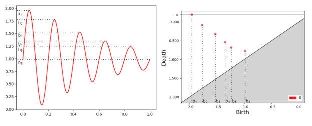
Figure 1: 1D illustration of the link between local maxima and $H_{0}$ persistence diagram. The birth times $b_{1}$, …, $b_{6}$ corresponds to the local maxima of the function.

The estimation of persistence diagram of a density is an interesting question by itself. A common approach (see e.g. Bubenik et al., 2009) in persistence diagram estimation is to use sup-norm (or other popular functional norm) stability theorem (Chazal et al., 2009) to lift convergence results for density (or signal) estimation in sup norm. This approach is limited as it supposes to be able to consistently estimate the density (or the signal) in sup-norm, which will typically fail under the local assumptions designed for modes estimation cited earlier. Bobrowski et al. (2017) proposed to break free from this approach, allowing to consider estimation of persistence diagram for a wide class of functions ($q-$tame functions). Unfortunately, this work does not quantify convergence rates. Under the same motivation, for the Gaussian white noise model and the non-parametric regression, in Henneuse (2024) we studied classes of piecewise Hölder functions tolerating irregularities that are difficult to handle for signal estimation. But on which it is still possible to infer persistence diagrams with convergence rates following the minimax one classically known on Hölder spaces. The proposed procedure in this work is based on histogram estimation of the (sub or super) level sets. We believe that these level sets estimators contains significantly more information than the one contained in persistence diagrams. In particular, we illustrate it in this work, showing that they contain the missing information to move from persistence diagram estimation to modes inference.

We here precise and discuss the settings considered in this paper. Let $f:[0,1]^{d}\rightarrow\mathbb{R}$ a probability density, we suppose that we observe $X=\{X_{1},...,X_{n}\}$ points sampled from $\mathbb{P}_{f}$.

Regularity assumptions on the densities are inspired by the one consider in Henneuse (2024) (adapted for super level filtration). A notable difference is that we relax the positive reach assumption made there into a positive $\mu-$reach assumption. This allows considerably wilder discontinuities sets, tolerating multiple points (i.e. self intersections of the discontinuities set) and corners. For a set $A\subset[0,1]^{d}$, $\overline{A}$ we denote its adherence and $\partial A$ its boundary. We consider the following assumptions over $f$ :

• A1. f is a piecewise $(L,\alpha)-$Hölder-continuous probability density, i.e. there exist $M_{1},...,M_{l}$ open sets of $[0,1]^{d}$ such that,

  $$\bigcup\limits_{i=1}^{l}\overline{M_{i}}=[0,1]^{d}$$

  and $f|_{M_{i}}$ is in $H(L,\alpha)$, $\forall i\in\{1,...,l\}$, with,

  $$H(L,\alpha)=\left\{f:[0,1]^{d}\rightarrow\mathbb{R}\text{ s.t. }|f(x)-f(y)|\leq L\|x-y\|_{2}^{\alpha},\forall x,y\in[0,1]^{d}\right\}.$$

  Assumption A1 control, on each $M_{i}$, how $f$ is “spiky”. The smaller the value of $\alpha$, the less mass there is around modes, making it more challenging to infer local maxima accurately.

• A2. $f$ verifies, $\forall x_{0}\in[0,1]^{d}$,

  $$\underset{x\in\bigcup\limits_{i=1}^{l}M_{i}\rightarrow x_{0}}{\limsup}f(x)=f(x_{0}).$$

  In this context, two signals, differing only on a null set, are statistically undistinguishable. Persistent homology is sensitive to point-wise irregularity, two signals differing only on a null set can have persistence diagrams that are arbitrarily far. Assumption A2 prevents such scenario.

• A3. Let $\mu\in]0,1]$ and $R_{\mu}>0$, for all $I\subset\{1,...,l\}$

  $$\operatorname{reach}_{\mu}\left(\bigcup\limits_{i=1}^{l}\partial M_{i}\right)\geq R_{\mu}.$$

  Here $\operatorname{reach}_{\mu}$ denotes the $\mu-$reach (defined by (1) in Section 1). $\mu-$reach is a generalization of the reach (Federer, 1959), introduced by Chazal et al. (2006). This can be though as geometric characterization of the regularity of the discontinuities set. The combination of Assumptions A3 and A1 ensures that at all point $x\in[0,1]^{d}$ there is a small half cone of apex $x$ and angles $2\cos^{-1}(\mu)$ on which $f$ is $(L,\alpha)-$Hölder. Following the remark made on A1, it gives control over the mass of the density around modes. We invite the reader to see Section 1, where we recall the definition of the $\mu-$reach and make additional remarks about Assumption A3.

The class of function verifying A1, A2 and A3 is denoted $S_{d}(L,\alpha,\mu,R_{\mu})$. As proved in Appendix D, densities in $S_{d}(L,\alpha,\mu,R_{\mu})$ have well-defined persistence diagram. We prove in this work that these assumptions are sufficient to infer the $H_{0}-$persistence diagram coming from the super level sets of $f$ consistently. For modes estimation, we require an additional assumption :

• A4. Let $h_{0}>0$, $0<C<L$ and $0<\alpha\leq 1$, for any $x$ local maxima of $f$ and $y\in B_{2}(x,h_{0})$,

  $$C\|x-y\|^{\alpha}_{2}\leq\|f(x)-f(y)\|_{2}.$$

  This assumption is common in the context of modes inference (Donoho and Liu, 1991; Dasgupta and Kpotufe, 2014; Jiang and Kpotufe, 2017; Arias-Castro et al., 2022). It has several implications. First, it ensures that local maxima are strict (modal sets are here singletons). Secondly, it ensures that the modes are well separated (at distance at least $h_{0}$) and that $f$ is not too flat around modes. The larger the value of $\alpha$, the more $f$ flattens around modes, making it more challenging to locate modes accurately.
  Moreover, denotes $l=Ch_{0}^{\alpha}$ and $\operatorname{dgm}(f)$ the $H_{0}-$persistence diagram of $f$, we have,

  $$\inf\limits_{(b,d)\in\operatorname{dgm}\left(f\right)}d-b\geq l.$$

  Thus A4 ensures that $\operatorname{dgm}(f)$ contains no point at distant less than $l$ from the diagonal, i.e. the magnitude of the modes is lower bounded by $l$. It consequently avoids having arbitrarily small oscillations and undetectable modes.

The class of function verifying A1, A2, A3 and A4 is denoted $S_{d}(L,\alpha,\mu,R_{\mu},C,h_{0})$.

Contribution

First, we propose a procedure based on histogram to estimate $H_{0}$-persistence diagram. We show that the proposed estimators achieves minimax rates over $S_{d}(L,\alpha,\mu,R_{\mu})$. The obtained convergence rates coincide with the known minimax ones over Hölder spaces. Secondly, taking advantage of this new results on persistence diagram estimation, we derive estimation procedures to infer the number of the modes, the localization of the modes and the values of $f$ at the modes. We show that these estimators are (up to a logarithmic factor) minimax over $S_{d}(L,\alpha,\mu,R_{\mu},C,h_{0})$. These results provide a formal framework and a rigorous study of convergence properties for inference of multiple modes based on persistence. It departs from existing statistical study, considering new sets of assumptions. Typically, in comparison to the conditions imposed in Dasgupta and Kpotufe (2014), our conditions are stronger globally (the densities being piecewise Hölder) but weaker locally (tolerating non differentiability or even discontinuities around modes). To illustrate this point, we provide some numerical illustrations in dimension 1 and 2.

The paper is organized as follows. Section 1 provides background on the geometric and topological concepts employed in this work. Section 2 is dedicated to $H_{0}-$persistence diagram estimation. Section 3 is dedicated to multiple modes estimation. And finally, Section 4 provides numerical illustrations. Proofs of technical lemmas and auxiliary results can be found in Appendix.

1 Background

This section provides the necessary background to follow this paper.

1.1 Distance function, generalized gradient and $\mu$-reach

We here present some concepts from geometric measure theory, used in this paper to control the geometry of the discontinuities set. Let $K\subset[0,1]^{d}$ a compact set, the distance function $d_{K}$ is given by,

$$d_{K}:x\mapsto\min\limits_{y\in K}||x-y||_{2}.$$

Generally the distance function is not differentiable everywhere, but we can define a generalized gradient function that matches with the gradient at points where the distance function is differentiable. Consider the set of closest point to $x$ in $K$,

$$\Gamma_{K}(x)=\{y\in K\mid||x-y||_{2}=d_{K}(x)\}$$

and for $x\in[0,1]^{d}\setminus K$, let $\Theta_{K}(x)$ the center of the unique smallest ball enclosing $\Gamma_{K}(x)$, the generalized gradient function $\nabla_{K}(x)$ is then defined as,

$$\nabla_{K}(x)=\frac{x-\Theta_{K}(x)}{d_{k}(x)}.$$

Figure 2: 2D example with 2 closest points

We can now introduce the notion of $\mu-$reach (Chazal et al., 2006), involved in assumptions A3. Let $K\subset[0,1]^{d}$ a compact set, its $\mu$-reach $\operatorname{reach}_{\mu}(K)$ is defined by,

$$\operatorname{reach}_{\mu}(K)=\inf\left\{r\mid\inf_{d_{K}^{-1}(r)}\left\|\nabla_{K}\right\|_{2}<\mu\right\}.$$ (1)

For $\mu=1$, this simply corresponds to the reach (Federer, 1959). The $\mu-$reach is positive for a large class of sets. For example, all piecewise linear compact sets have positive $\mu-$reach (for some $\mu$). In our context, considering the $\mu-$reach instead of the reach in assumption A3 allow considering a significantly wider class of irregular densities, tolerating corners and multiple points.

(a) Positive ($1-$)reach

(b) Positive $\mu-$reach ($\mu$ small)

Figure 3: (a) display a partition $M_{1}$,…, $M_{6}$ such that $\operatorname{reach}_{1}\left(\partial M_{1}\cup...\cup\partial M_{6}\right)>0$. (b) display a partition $M_{1}$,…, $M_{6}$ such that $\operatorname{reach}_{1}\left(\partial M_{1}\cup...\cup\partial M_{6}\right)=0$ (in red are highlighted problematic points) but for sufficiently small $\mu>0$, $\operatorname{reach}_{\mu}\left(\partial M_{1}\cup...\cup\partial M_{6}\right)>0$.

Another way to understand the $\mu-$reach is to see it as the distance from the $\mu-$medial axis. The $\mu-$medial axis of a set $K\subset[0,1]^{d}$ is defined by,

$$\operatorname{Med}_{\mu}(K)=\left\{x\in[0,1]^{d}\quad|\quad\|\nabla_{K}(x)\|_{2}<\mu\right\}.$$

The $\mu-$reach of $K$ then being equal to $d_{2}(K,\overline{\operatorname{Med}_{\mu}(K)})$.

Figure 4: Illustration of $\mu-$medial axis for a set $K$. In black is represented the $1-$medial axis, in red the $0-$medial axis and in blue the $\mu-$medial axis for a small $0<\mu<1/2$.

1.2 Filtration, persistence module and $H_{0}$-persistence diagram

We here present briefly some notions related to persistence homology. Persistent homology permits to encode the evolution of topological features (in the homology sense) along a family of nested spaces, called filtration. Moving along indices, topological features (connected components, cycles, cavities, …) can appear or die (existing connected components merge, cycle or cavities are filled, …). In this paper, we focus on $H_{0}-$persistent homology, that describe the evolution of connectivity. For a broader overview and visual illustrations of persistent homology, we recommend Chazal and Michel (2021). For detailed and rigorous constructions, see Chazal et al. (2016). Additionally, since the construction discussed here involves (singular) homology, the reader can refer to Hatcher (2000).

The typical filtration that we will consider in this paper is, for a function $f:\mathbb{R}^{d}\rightarrow\mathbb{R}$, the family of superlevel sets $\left(\mathcal{F}_{\lambda}\right)_{\lambda\in\mathbb{R}}=\left(f^{-1}([\lambda,+\infty[)\right)_{\lambda\in\mathbb{R}}$. The associated family of homology group of degree $0$, $\mathbb{V}_{f,0}=\left(H_{0}\left(\mathcal{F}_{\lambda}\right)\right)_{\lambda\in\mathbb{R}}$, equipped with $v_{\lambda}^{\lambda^{{}^{\prime}}}$ the linear application induced by the inclusion $\mathcal{F}_{\lambda}\subset\mathcal{F}_{\lambda^{\prime}}$, for all $\lambda>\lambda^{{}^{\prime}}$ forms a persistence module. To be more precise, in this paper, $H_{0}(.)$ is the singular homology functor in degree $0$ with coefficient in a field (typically $\mathbb{Z}/2\mathbb{Z}$). Hence, $H_{0}\left(\mathcal{F}_{\lambda}\right)$ is a vector space.

if $\forall\lambda>\lambda^{\prime}\in\mathbb{R}$, $\operatorname{rank}(v_{\lambda}^{\lambda^{\prime}})$ is finite, the module is said to be $q-$tame. It is then possible to show that the algebraic structure of the persistence module encodes exactly the evolution of the topological features along the filtration. For details, we encourage the reader to look at Chazal et al. (2016). Furthermore, the algebraic structure of a such persistence module can be summarized by a collection $\{(b_{i},d_{i}),i\in I\}\subset\overline{\mathbb{R}}^{2}$, which defined the persistence diagram. Following previous remarks, for $H_{0}-$persistent homology, $b_{i}$ corresponds to the birth time of a connected component, $d_{i}$ corresponds to its death time and $d_{i}-b_{i}$ to its lifetime.

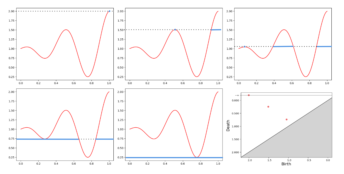
Figure 5: Super level sets filtration of $f(x)=x\cos(4\pi x)$ over $[0,1]$ and the associated $H_{0}$ persistence-diagram.

To compare persistence diagrams, a popular distance, especially in statistical context, is the bottleneck distance, defined for two persistence diagrams $D_{1}$ and $D_{2}$ by,

$$d_{b}\left(D_{1},D_{2}\right)=\underset{\gamma\in\Gamma}{\inf}\underset{p\in D_{1}}{\sup}||p-\gamma(p)||_{\infty}$$

with $\Gamma$ the set of all bijection between $D_{1}$ and $D_{2}$ (both enriched with the diagonal).

We now present the algebraic stability theorem for the bottleneck distance. This theorem was the key for proving upper bounds in Henneuse (2024), it is also the case in this work to establish our main results. This theorem relies on interleaving between modules, a notion we extensively exploit. Let $f:[0,1]^{d}\rightarrow\mathbb{R}$ and $g:[0,1]^{d}\rightarrow\mathbb{R}$, the associated $H_{0}-$persistent modules for the superlevel sets filtrations, denoted respectively $\mathbb{V}$ and $\mathbb{W}$, are said to be $\varepsilon$-interleaved if there exists two families of applications $\phi=\left(\phi_{\lambda}\right)_{\lambda\mathbb{R}}$ and $\psi=\left(\psi_{\lambda}\right)_{\lambda\mathbb{R}}$ where $\phi_{\lambda}:\mathbb{V}_{\lambda}\rightarrow\mathbb{W}_{\lambda-\varepsilon}$, $\psi_{\lambda}:\mathbb{V}_{\lambda}\rightarrow\mathbb{W}_{\lambda-\varepsilon}$, and for all $\lambda>\lambda^{{}^{\prime}}$ the following diagrams commutes,

(2)

Theorem (Chazal et al. 2009, "algebraic stability").

Let $\mathbb{V}$ and $\mathbb{W}$ two $q-$tame persistence modules. If $\mathbb{V}$ and $\mathbb{W}$ are $\varepsilon-$interleaved then,

$$d_{b}\left(\operatorname{dgm}(\mathbb{V}),\operatorname{dgm}(\mathbb{W})\right)\leq\varepsilon.$$

A direct corollary of this result, proved earlier in special cases (Barannikov, 1994; Cohen-Steiner et al., 2005), is the sup-norm stability of persistence diagrams. We insist on the fact that this is a strictly weaker result than algebraic stability.

Theorem ("sup norm stability").

Let $f$ and $g$ two real-valued function and $s\in\mathbb{N}$. If their persistent modules for the $s-th$ order homology, denoted $\mathbb{V}$ and $\mathbb{W}$, are $q-$tame, then,

$$d_{b}\left(\operatorname{dgm}\left(\mathbb{V}\right),\operatorname{dgm}\left(\mathbb{W}\right)\right)\leq||f-g||_{\infty}.$$

As highlighted in the introduction, the sup-norm stability is often used to upper bounds the errors in bottleneck distance of "plug-in" estimators of persistence diagrams. It enables the direct translation of convergence rates in sup-norm to convergence rates in bottleneck distance, which for regular classes of signals provides minimax upper bounds. But, for wider classes, this approach falls short.

(a) graphs of $f_{0}$ and $f_{1}$

(b) persistence diagrams of $f_{0}$ and $f_{1}$

Figure 6: 1D Illustration of stability theorems.

2 $H_{0}-$persistence diagram estimation

This section describes our procedure for persistence diagram estimation and provides associated convergence results.

2.1 Procedure description

We propose a procedure to estimate $H_{0}-$persistence diagram over $S_{d}(L,\alpha,\mu,R_{\mu},C,h_{0})$. Contrary to the setting of Henneuse (2024), where the positive reach assumptions allows considering plug-in estimation directly through histogram, under the weaker assumptions made here, this approach falls short as illustrated in figure 7. To recover properly the connectivity of the sublevel sets filtration, we need an additional thickening.

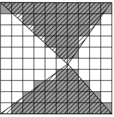
Figure 7: $\lambda-$superlevel cubical approximation for $f$ the function defined as $0$ outside the hatched area and $K$ inside (for arbitrarily large $K$). The histogram approximation fails to identify the connectivity of the two triangle for at least all $3K/4<\lambda<K$.

Let denote,

$$A^{b}=\left\{x\in\mathbb{R}^{d}\text{ s.t. }d_{\infty}\left(x,A\right)\leq b\right\}$$

with

$$d_{\infty}\left(x,A\right)=\inf\limits_{y\in A}||x-y||_{\infty}.$$

Let $h>0$ such that $1/h$ is an integer, consider $G(h)$ the regular orthogonal grid over $[0,1]^{d}$ of step $h$ and $C_{h}$ the collection of all the hypercubes of side $h$ composing $G(h)$. We define, $\forall\lambda\in\mathbb{R}$, the $\lambda-$sublevel estimator,

$$\widehat{\mathcal{F}}_{\lambda}=\left(\bigcup\limits_{H\in C_{h,\lambda}}H\right)^{\lceil\sqrt{d}/\mu\rceil h}\text{ with }C_{h,\lambda}=\left\{H\in C_{h}\text{ such that }\frac{|X\cap H|}{nh^{d}}\geq\lambda\right\}$$

with $\lceil.\rceil$ the ceiling function. Let $\lambda>\lambda^{{}^{\prime}}$, we denote,

$$\hat{v}_{\lambda}^{\lambda^{{}^{\prime}}}:H_{0}\left(\widehat{\mathcal{F}}_{\lambda}\right)\rightarrow H_{0}\left(\widehat{\mathcal{F}}_{\lambda^{{}^{\prime}}}\right)$$

the map induced by the inclusion $\widehat{\mathcal{F}}_{\lambda}\subset\widehat{\mathcal{F}}_{\lambda^{{}^{\prime}}}$. We now introduce $\widehat{\mathbb{V}}_{f,0}$ the persistence module associated to $(H_{0}(\widehat{\mathcal{F}}_{\lambda}))_{\lambda\in\mathbb{R}}$ equipped with the collection of maps $(\widehat{v}_{\lambda,h}^{\lambda^{{}^{\prime}}})_{\lambda>\lambda^{{}^{\prime}}}$ and $\widehat{\operatorname{dgm}(f)}$ the associated $H_{0}-$persistence diagram. These diagrams are well-defined, as we prove in Appendix D that $\widehat{\mathbb{V}}_{f,0}$ is $q-$tame.

Calibration. A natural question is how to choose the parameter $h$. Following the proof of Lemma 2, we choose $h$ verifying,

$$h>\sqrt{\frac{\log\left(1/h^{d}\right)}{nh^{d}}}$$ (3)

In particular, we can choose,

$$h\simeq\left(\frac{\log(n)}{n}\right)^{\frac{1}{d+2\alpha}}.$$

Computation. By construction, for all $\lambda\in\mathbb{R}$, $\widehat{\mathcal{F}}_{\lambda}$ is simply a union of cubes from the regular grid $G(h)$, thus can be thought as a (geometric realization of) a cubical complex or even a simplicial complex. Hence, it allows practical computation of its persistence diagram.

2.2 Convergence Rates

In this section, we state our main results concerning persistence diagram estimation, Theorem 1 and Theorem 2, establishing that the procedure proposed in the previous section achieves minimax rates over $S_{d}(L,\alpha,\mu,R_{\mu})$.

Theorem 1.

Let $h\simeq\left(\frac{\log(n)}{n}\right)^{\frac{1}{d+2\alpha}}$. There exists $\tilde{C}_{0}$ and $\tilde{C}_{1}$ such that, for all $A\geq 0$,

$$\mathbb{P}\left(\sup\limits_{f\in S(L,R,\alpha)}d_{\infty}\left(\widehat{\operatorname{dgm}(f)},\operatorname{dgm}(f)\right)\geq A\left(\frac{\log(n)}{n}\right)^{\frac{\alpha}{d+2\alpha}}\right)\leq\tilde{C}_{0}\exp\left(-\tilde{C}_{1}A^{2}\right).$$

From this, we can derive from this result a bound in expectation.

Corollary 1.

Let $h\simeq\left(\frac{\log(n)}{n}\right)^{\frac{1}{d+2\alpha}}$ and $p\geq 1$,

$$\underset{f\in S(L,R,\alpha)}{\sup}\quad\mathbb{E}\left(d_{\infty}\left(\widehat{\operatorname{dgm}(f)},\operatorname{dgm}(f)\right)^{p}\right)\lesssim\left(\frac{\log(n)}{n}\right)^{\frac{p\alpha}{d+2\alpha}}$$

Proof.

The sub-Gaussian concentration provided by Proposition 1, gives that, for all $A\geq 0$,

$$\mathbb{P}\left(\frac{d_{b}\left(\widehat{\operatorname{dgm}(f)},\operatorname{dgm}(f)\right)}{h^{\alpha}}\geq A\right)\leq\tilde{C}_{0}\exp\left(-\tilde{C}_{1}A^{2}\right).$$

Now, we have,

$$\quad\mathbb{E}\left(\frac{d_{b}\left(\widehat{\operatorname{dgm}(f)},\operatorname{dgm}(f)\right)^{p}}{h^{p\alpha}}\right) =\int_{0}^{+\infty}\mathbb{P}\left(\frac{d_{b}\left(\widehat{\operatorname{dgm}(f)},\operatorname{dgm}(f)\right)^{p}}{h^{p\alpha}}\geq A\right)dA$$

$$\leq\int_{0}^{+\infty}\tilde{C}_{0}\exp\left(-\tilde{C}_{1}A^{\nicefrac{{2}}{{p}}}\right)dA<+\infty.$$

∎

Theorem 2.

Let $p\geq 1$

$$\underset{\widehat{\operatorname{dgm}(f)}}{\inf}\quad\underset{f\in S_{d}(L,\alpha,\mu,R_{\mu})}{\sup}\quad\mathbb{E}\left(d_{\infty}\left(\widehat{\operatorname{dgm}(f)},\operatorname{dgm}(f)\right)^{p}\right)\gtrsim\left(\frac{\log(n)}{n}\right)^{\frac{p\alpha}{d+2\alpha}}$$

Where the infimum is taken over all the estimator of $\operatorname{dgm}(f)$.

2.3 Proof of Theorem 1

This section is devoted to the proofs of Theorem 1 and Corollary 1 stated in Section 2.2. The idea is to construct an interleaving between $\mathbb{V}_{f,0}$ and $\widehat{\mathbb{V}}_{f,0}$, to then apply the algebraic stability theorem Chazal et al. (2009). This requires to construct two morphism $\overline{\psi}:\mathbb{V}_{f,0}\rightarrow\widehat{\mathbb{V}}_{f,0}$ and $\overline{\phi}:\widehat{\mathbb{V}}_{f,0}\rightarrow\mathbb{V}_{f,0}$ satisfying (2). The following sections give the necessary ingredients.

2.3.1 Ingredient 1 : inclusions between level sets

If there existed an $\varepsilon>0$ such that for all $\lambda\in\mathbb{R}$, $\mathcal{F}_{\lambda}\subset\widehat{\mathcal{F}}_{\lambda-\varepsilon}\subset\mathcal{F}_{\lambda-2\varepsilon}$, an $\varepsilon-$interleaving would be directly given taking the morphisms induced by inclusions. Here we do not have such nice inclusions, but we show, in Proposition 1, a slightly weaker double inclusion.

First remark that the $f\in S_{d}\left(L,\alpha,\mu,R_{\mu}\right)$ are uniformly bounded, as stated in the following lemma, which proof can be found in Appendix C.

Lemma 1.

Let $f\in S_{d}\left(L,\alpha,\mu,R_{\mu}\right)$, there exists a constant $M_{d,L,R_{\mu}}$ depending on $d$, $L$ and $R_{\mu}$, such that $\|f\|_{\infty}\leq M_{d,L,R_{\mu}}$.

And denotes, $N_{h}$ the variable defined by,

$$N_{h}=\frac{\max\limits_{H\in C_{h}}\left|\frac{|X\cap H|}{nh^{d}}-\mathbb{E}\left[\frac{|X\cap H|}{nh^{d}}\right]\right|}{\sqrt{3M_{d,L,R_{\mu}}\frac{\log\left(1/h^{d}\right)}{nh^{d}}}}$$

Proposition 1.

Let $f\in S_{d}\left(L,\alpha,\mu,R_{\mu}\right)$ and $h\simeq\left(\nicefrac{{\log(n)}}{{n}}\right)^{\frac{1}{d+2\alpha}}$. For $n$ sufficiently large such that $h<R_{\mu}/\sqrt{d}$, for all $\lambda\in\mathbb{R}$, we have,

$$\mathcal{F}_{\lambda+\left(2\sqrt{3M_{d,L,R_{\mu}}}N_{h}+L\left(\lceil\sqrt{d}/\mu\rceil+\sqrt{d}\right)^{\alpha}\right)h^{\alpha}}\subset\widehat{\mathcal{F}}_{\lambda}\subset\mathcal{F}_{\lambda-2\sqrt{3M_{d,L,R_{\mu}}}N_{h}h^{\alpha}}^{(\sqrt{d}+\lceil\sqrt{d}/\mu\rceil)h}.$$

This proposition then follows from Lemma 3.1 from Chazal et al. (2007) and the following lemma, which proof can be found in Appendix B.

Lemma 2.

Let $f\in S_{d}(L,\alpha,\mu,R_{\mu})$ and $h>0$ verifying (3). Let

$$H\subset\mathcal{F}_{\lambda-2\sqrt{3M_{d,L,R_{\mu}}}N_{h}h^{\alpha}}^{c}\cap C_{h}$$

and

$$H^{{}^{\prime}}\subset\mathcal{F}_{\lambda+2\sqrt{3M_{d,L,R_{\mu}}}N_{h}h^{\alpha}}\cap C_{h}.$$

We then have that,

$$\frac{|X\cap H|}{nh^{d}}<\lambda\text{ and }\frac{|X\cap H^{{}^{\prime}}|}{nh^{d}}>\lambda.$$

For a set $K\subset[0,1]^{d}$ and $r\geq 0$ we denote $B_{2}(K,r)=\{x\in[0,1]^{d}\text{ s.t. }d_{K}(x)<r\}$ and $\overline{B}_{2}(K,r)=\{x\in[0,1]^{d}\text{ s.t. }d_{K}(x)\leq r\}$.

Lemma 3.

(Chazal et al., 2007, Lemma 3.1.) Let $K\subset[0,1]^{d}$ a compact set and let $\mu>0,r>0$ be such that $r<\operatorname{reach}_{\mu}(K)$. For any $x\in\overline{B}_{2}(K,r)\backslash K$, we have,

$$d_{2}\left(x,\partial\overline{B}_{2}(K,r)\right)\leq\frac{r-d_{K}(x)}{\mu}\leq\frac{r}{\mu}.$$

Proof of Proposition 1.

We begin by proving the lower inclusion, let,

$$x\in\mathcal{F}_{\lambda+\left(2\sqrt{3M_{d,L,R_{\mu}}}N_{h}+L\left(\lceil\sqrt{d}/\mu\rceil+\sqrt{d}\right)^{\alpha}\right)h^{\alpha}}.$$

Without loss of generality, let suppose $x\in\overline{M}_{i}$. If,

$$B_{2}\left(x,\sqrt{d}h\right)\subset\left(\bigcup\limits_{i=1}^{l}\partial M_{i}\right)^{c}$$

then, $H_{x,h}$, the hypercube of $C_{h,\lambda}$ containing $x$ is included in $\overline{M}_{i}$. Assumption A1 and A2 then gives $H_{x,h}\subset\mathcal{F}_{\lambda+2\sqrt{3M_{d,L,R_{\mu}}}N_{h}h^{\alpha}}$. Hence, it follows from Lemma 2 that $H_{x,h}\in C_{h,\lambda}$ and consequently $x\in\widehat{\mathcal{F}}_{\lambda}$. Else, under Assumption A3, by Lemma 3, there exists,

$$y\in\left(\left(\bigcup\limits_{i=1}^{l}\partial M_{i}\right)^{\sqrt{d}h}\right)^{c}\cap M_{i}\text{ such that }||x-y||_{2}\leq\sqrt{d}h/\mu.$$

Let $H_{y,h}$ the closed hypercube of $C_{h}$ containing $y$. Hence, $H_{y,h}\subset\overline{M_{i}}.$ and $d_{2}\left(x,H_{y,h}\right)\leq\sqrt{d}h(1+1/\mu)$. Then, Assumption A1 and A2 ensures that,

$$H_{y,h}\subset\mathcal{F}_{\lambda+2\sqrt{3M_{d,L,R_{\mu}}}N_{h}h^{\alpha}}.$$

Then, Lemma 2 gives $H_{y,h}\in C_{h,\lambda}$ and thus, as $x\in H_{y,h}^{\sqrt{d}h/\mu}$, $x\in\widehat{\mathcal{F}}_{\lambda}$, which proves the lower inclusion.

For the upper inclusion, let $x\in\left(\mathcal{F}_{\lambda-2\sqrt{3M_{d,L,R_{\mu}}}N_{h}h^{\alpha}}^{\sqrt{d}h}\right)^{c}$, and $H_{x,h}$ the hypercube of $C_{h}$ containing $x$. We then have, $H_{x,h}\subset\mathcal{F}_{\lambda-2\sqrt{3M_{d,L,R_{\mu}}}N_{h}h^{\alpha}}^{c}$. Hence, Lemma 2 gives that,

$$H_{x,h}\subset\left(\bigcup\limits_{H\in C_{h,\lambda}}H\right)^{c}$$

and thus,

$$\bigcup\limits_{H\in C_{h,\lambda}}H\subset\mathcal{F}_{\lambda-2\sqrt{3M_{d,L,R_{\mu}}}N_{h}h^{\alpha}}^{\sqrt{d}h}.$$

Consequently,

$$\left(\bigcup\limits_{H\in C_{h,\lambda}}H\right)^{\lceil\sqrt{d}/\mu\rceil h}=\widehat{\mathcal{F}}_{\lambda}\subset\mathcal{F}_{\lambda-2\sqrt{3M_{d,L,R_{\mu}}}N_{h}h^{\alpha}}^{(\sqrt{d}+\lceil\sqrt{d}/\mu\rceil)h}$$

and the proof is complete. ∎

2.3.2 Ingredient 2 : geometry of thicken level sets

The lower inclusion of Proposition 1 gives directly a morphism $\overline{\psi}:\mathbb{V}_{f,0}\rightarrow\widehat{\mathbb{V}}_{f,0}$. But the upper inclusion is not sufficient to provides similarly $\overline{\phi}:\widehat{\mathbb{V}}_{f,0}\rightarrow\mathbb{V}_{f,0}$. To overcome this issue, in Proposition 2, we exploit assumption A3 to construct morphisms from $(H_{0}(\mathcal{F}_{\lambda}^{r}))_{\lambda\in\mathbb{R}}$ into $V_{f,0}$, for all $r<R_{\mu}/\sqrt{d}$. For $r=(\sqrt{d}+\lceil\sqrt{d}/\mu\rceil)h$, composing this morphism with the one induced by the upper inclusion of Proposition 1 will give us our morphism $\overline{\phi}$.

Proposition 2.

Let $f\in S_{d}(L,\alpha,\mu,R_{\mu})$. $\forall s\in\mathbb{N}$, $\forall h<R_{\mu}/\sqrt{d}$, there exist a morphism $\phi$ such that, $\forall\lambda\in\mathbb{R}$,

(4)

is a commutative diagram (unspecified map come from set inclusions).

To prove this proposition, we use the following lemma. This result involves the notion of deformation retract that we recall here.

Definition 1.

A subspace $A$ of $X$ is called a deformation retract of $X$ if there is a continuous $F:X\times[0,1]\rightarrow X$ such that for all $x\in X$ and $a\in A$,

• $F(x,0)=x$

• $F(x,1)\in A$

• $F(a,1)=a$.

The function $x\mapsto F(x,1)$ is called a (deformation) retraction from $X$ to $A$.

Lemma 4.

(Kim et al., 2020, Theorem 12) Let $K\subset[0,1]^{d}$, for all $0\leq r<\operatorname{reach}_{\mu}(K)$, $B_{2}(K,r)$ retracts by deformation onto $K$ and the associated retraction $R:B_{2}(K,r)\rightarrow K$ verifies for all $x\in B_{2}(K,r)$, $R(x)\in B_{2}(x,2r/\mu^{2})$.

The first part of the claim is Theorem 12 from Kim et al. (2020) and the second part follows easily from their construction. Elements of proof can be found in Appendix A.

Proof of Proposition 2.

Any connected components $B$ of $\mathcal{F}_{\lambda}^{h}$ contains at least a connected component $A$ of $\mathcal{F}_{\lambda}$. Suppose that $B$ contains $A$ and $A^{{}^{\prime}}$ two disjoint connected components of $\mathcal{F}_{\lambda}$, then there exists $x\in A$ and $y\in A^{{}^{\prime}}$ such that $||x-y||_{\infty}\leq 2h$. Suppose that $x\in M_{i}$ and $y\in M_{j}$, $i,j\in\{1,...,l\}$.

If the segment $[x,y]$ is included in $\bar{M}_{i}\cup\bar{M}_{j}$, then by Assumptions A1 and A2, directly we have $[x,y]\subset\mathcal{F}_{\lambda-L(2\sqrt{d}h)^{\alpha}}$ and thus $A$ and $A^{{}^{\prime}}$ are connected in $\mathcal{F}_{\lambda-L(2\sqrt{d}h)^{\alpha}}$.

Otherwise, there exists $\bar{x}\in\partial M_{i}$ and $\bar{y}\in\partial M_{j}$ such that $[\bar{x},\bar{y}]\subset(M_{i}\cup M_{j})^{c}$ and $[x,y]\setminus[\bar{x},\bar{y}]\subset M_{i}\cup M_{j}$. It follows from Assumptions A1 that $[x,y]\setminus[\bar{x},\bar{y}]\subset\mathcal{F}_{\lambda-L(2\sqrt{d}h)^{\alpha}}$.
Now, let,

$$R:B_{2}(\partial M_{i}\cup\partial M_{j},\sqrt{d}h)\rightarrow\partial M_{i}\cup\partial M_{j}$$

the deformation retraction of $B_{2}(\partial M_{i}\cup\partial M_{j},\sqrt{d}h)$ onto $\partial M_{i}\cup\partial M_{j}$ given by Lemma 4 under Assumption A3. As $R(\bar{x})=\bar{x}$, $R(\bar{y})=\bar{y}$ and $R$ continuous, $R([\bar{x},\bar{y}])$ is a continuous path between $\bar{x}$ and $\bar{y}$.
Furthermore, also by Lemma 4, we have,

$$R([\bar{x},\bar{y}])\subset\left(\partial M_{i}\cup\partial M_{j}\right)\cap B_{2}([\bar{x},\bar{y}],2\sqrt{d}h/\mu^{2}).$$

Let $z\in R([\bar{x},\bar{y}])\cap M_{i}$ then, $z\in B_{2}(x,(2+2/\mu^{2})\sqrt{d}h)$ and thus by Assumptions A1 and A2, $z\in\mathcal{F}_{\lambda-L((2+2/\mu^{2})\sqrt{d}h)^{\alpha}}$.
Similarly, if $z\in R([\bar{x},\bar{y}])\cap M_{j}$ then, $z\in B_{2}(y,(2+2/\mu^{2})\sqrt{d}h)$ and $z\in\mathcal{F}_{\lambda-L((2+2/\mu^{2})\sqrt{d}h)^{\alpha}}$. Hence,

$$R([\bar{x},\bar{y}])\subset\mathcal{F}_{\lambda-L((2+2/\mu^{2})\sqrt{d}h)^{\alpha}}.$$

Thus, $[x,\bar{x}]\cup R([\bar{x},\bar{y}])\cup[\bar{y},\bar{x}]$ is a continuous path between $x$ and $y$, included in $\mathcal{F}_{\lambda-L((2+2/\mu^{2})\sqrt{d}h)^{\alpha}}$. And consequently, in this case also $A$ and $A^{{}^{\prime}}$ are connected in $\mathcal{F}_{\lambda-L((2+2/\mu^{2})\sqrt{d}h)^{\alpha}}$.

We can then properly define,

$$\left\{\begin{array}[]{ll}\phi_{\lambda}:H_{0}(\mathcal{F}_{\lambda}^{h})&\rightarrow H_{0}(\mathcal{F}_{\lambda-L((2+2/\mu^{2})\sqrt{d})^{\alpha}h^{\alpha}})\\ \quad\quad[x]&\longmapsto[y]\end{array}\right.$$

with $y$ belonging to $A$ any connected components of $\mathcal{F}_{\lambda}$ included in $B$, the connected component of $\mathcal{F}_{\lambda}^{h}$ containing $x$. By the foregoing, $[x]$ is independent of the choice of such $A$ (and such $y$ in $A$) and Diagram 4 commutes. ∎

2.3.3 Ingredient 3 : concentration of $N_{h}$

The two previous ingredients will permit to establish an interleaving between $\widehat{\mathbb{V}}_{f,0}$ and $\mathbb{V}_{f,0}$. This interleaving will depend on the variable $N_{h}$. Consequently, to derive convergence rates from this interleaving, we need concentration inequalities over $N_{h}$.

Proposition 3.

For all $h>0$,

$$\mathbb{P}\left(\bigcup\limits_{H\in C_{h}}\left|\frac{|X\cap H|}{nh^{d}}-\mathbb{E}\left[\frac{|X\cap H|}{nh^{d}}\right]\right|\geq t\right)\leq\frac{2}{h^{d}}\exp\left(-\frac{t^{2}nh^{d}}{3M_{d,L,R_{\mu}}}\right).$$

Proof of Proposition 3.

Let $h>0$ and $H\in C_{h}$. We can write,

$$|X\cap H|=\sum\limits_{i=1}^{n}Y_{i}^{H}$$

with, for all $i\in\{1,...,n\}$,

$$Y_{i}^{H}=\mathbb{1}_{X_{i}\in H}$$

As $X_{1},...,X_{n}$ are i.i.d., $Y_{1}^{H},...,Y_{n}^{H}$ are i.i.d. Bernoulli variable, and $|X\cap H|$ is then a Binomial variable of parameters $\left(n,P(X_{1}\in H)\right)$. It follows from the Chernoff bounds for binomial distribution that,

$$\mathbb{P}\left(\left|\frac{|X\cap H|}{nh^{d}}-\mathbb{E}\left[\frac{|X\cap H|}{nh^{d}}\right]\right|\geq t\right)\leq 2\exp\left(-\frac{t^{2}nh^{2d}}{3P(X_{1}\in H)}\right).$$

Lemma 1 then gives that $P(X_{1}\in H)\leq h^{d}M_{d,L,R_{\mu}}$, hence,

$$\mathbb{P}\left(\left|\frac{|X\cap H|}{nh^{d}}-\mathbb{E}\left[\frac{|X\cap H|}{nh^{d}}\right]\right|\geq t\right)\leq 2\exp\left(-\frac{t^{2}nh^{d}}{3M_{d,L,R_{\mu}}}\right).$$

By union bounds, it follows,

$$\mathbb{P}\left(\bigcup\limits_{H\in C_{h}}\left\{\left|\frac{|X\cap H|}{nh^{d}}-\mathbb{E}\left[\frac{|X\cap H|}{nh^{d}}\right]\right|\geq t\right\}\right)\leq 2\left|C_{h}\right|\exp\left(-\frac{t^{2}nh^{d}}{3M_{d,L,R_{\mu}}}\right)\leq\frac{2}{h^{d}}\exp\left(-\frac{t^{2}nh^{d}}{3M_{d,L,R_{\mu}}}\right).$$

∎

Proposition 3 implies that $N_{h}$ is sub Gaussian. More precisely, there exists two constant depending only on $d,L,R_{\mu}$, such that, for all $h$,

$$\mathbb{P}\left(N_{h}>t\right)\leq C_{0}\exp\left(-C_{1}t^{2}\right).$$

2.3.4 Main proof

Equipped with Proposition 1, 2 and 3 we can now proceed to the proof of Theorem 1.

Proof of Theorem 1.

It suffices to show the result for (arbitrarily) large $n$ (up to rescaling $\tilde{C_{0}}$), thus suppose that $n$ is sufficiently large for the application of Propositions 1 and 2 used in this proof. We denote $k_{1}=\sqrt{d}+\lceil\sqrt{d}/\mu\rceil$ and $k_{2}=\sqrt{d}\left(2+2/\mu^{2}\right)(\sqrt{d}+\lceil\sqrt{d}/\mu\rceil)$.

First, we construct $\overline{\phi}$. Let $\lambda\in\mathbb{R}$, Lemma 2 imply that any connected component $A$ of $\widehat{\mathcal{F}}_{\lambda}$ intersects a connected component $B$ of $\mathcal{F}_{\lambda-2\sqrt{3M_{d,L,R_{\mu}}}N_{h}h^{\alpha}}$. Now suppose that $A$ intersects 2 such components $B_{1}$ and $B_{2}$, then, by Proposition 1, $B_{1}$ and $B_{2}$ are connected in $\mathcal{F}_{\lambda-2\sqrt{3M_{d,L,R_{\mu}}}N_{h}h^{\alpha}}^{k_{1}h}$. Thus, as a consequence of Proposition 2, $B_{1}$ and $B_{2}$ are connected in $\mathcal{F}_{\lambda-\left(2\sqrt{3M_{d,L,R_{\mu}}}N_{h}+Lk_{2}^{\alpha}\right)h^{\alpha}}$. We can then define properly the applications,

$$\left\{\begin{array}[]{ll}\overline{\phi}_{\lambda}:H_{0}\left(\widehat{\mathcal{F}}_{\lambda}\right)&\longrightarrow H_{0}\left(\mathcal{F}_{\lambda-\left(2\sqrt{3M_{d,L,R_{\mu}}}N_{h}+Lk_{2}^{\alpha}\right)h^{\alpha}}\right)\\ \quad\quad[x]&\longmapsto[y]\end{array}\right.$$

with $y$ belonging to $B$ a connected component of $\mathcal{F}_{\lambda-2\sqrt{3M_{d,L,R_{\mu}}}N_{h}h^{\alpha}}$ intersecting $A$, the connected components containing $x$. The previous remark ensures that $[y]$ is independent of the choice of $B$.

Now, for the construction of $\overline{\psi}$, by Proposition 1, we have,

$$\mathcal{F}_{\lambda}\subset\widehat{\mathcal{F}}_{\lambda-\left(2\sqrt{3M_{d,L,R_{\mu}}}N_{h}+Lk_{1}^{\alpha}\right)h^{\alpha}}$$

and we simply take $\overline{\phi}$ the morphism induced by this inclusion, i.e,

$$\left\{\begin{array}[]{ll}\overline{\psi}_{\lambda}:H_{0}\left(\mathcal{F}_{\lambda}\right)&\longrightarrow H_{0}\left(\widehat{\mathcal{F}}_{\lambda-\left(2\sqrt{3M_{d,L,R_{\mu}}}N_{h}+Lk_{1}^{\alpha}\right)h^{\alpha}}\right)\\ \quad\quad[x]&\longmapsto[x]\end{array}\right.$$

Denote $\tilde{K}_{1}=2\sqrt{3M_{d,L,R_{\mu}}}N_{h}+Lk_{1}^{\alpha}$ and $\tilde{K}_{2}=2\sqrt{3M_{d,L,R_{\mu}}}N_{h}+Lk_{2}^{\alpha}$. The foregoing ensures the commutativity of following diagrams (unspecified maps are the one induced by set inclusion),

Hence $\widehat{\mathbb{V}}_{f,0}$ and $\mathbb{V}_{f,0}$ are $(\tilde{K}_{1}+\tilde{K}_{2})h^{\alpha}$-interleaved, and thus we get from the algebraic stability theorem (Chazal et al., 2009) that,

$$d_{b}\left(\operatorname{dgm}\left(\widehat{\mathbb{V}}_{f,0}\right),\operatorname{dgm}\left(\mathbb{V}_{f,0}\right)\right)\leq(K_{1}+K_{2})h^{\alpha}$$

and as it holds for all $f\in S_{d}(L,\alpha,\mu,R_{\mu})$,

$$\sup\limits_{f\in S_{d}(L,\alpha,\mu,R_{\mu})}d_{b}\left(\widehat{\operatorname{dgm}(f)},\operatorname{dgm}(f)\right)\leq(K_{1}+K_{2})h^{\alpha}.$$

We then conclude, using the concentration of $N_{h}$ given in Proposition 3.

$$\mathbb{P}\left(\sup\limits_{f\in S_{d}(L,\alpha,\mu,R_{\mu})}d_{b}\left(\widehat{\operatorname{dgm}(f)},\operatorname{dgm}(f)\right)\geq th\right)$$

$$\leq\mathbb{P}\left(K_{1}+K_{2}\geq t\right)$$

$$=\mathbb{P}\left(N_{h}\geq\frac{t-L\left(k_{1}^{\alpha}+k_{2}^{\alpha}\right)}{4\sqrt{3M_{d,L,R_{\mu}}}}\right)$$

$$\leq C_{0}\exp\left(-C_{1}\left(\frac{t-L\left(k_{1}^{\alpha}+k_{2}^{\alpha}\right)}{4\sqrt{3M_{d,L,R_{\mu}}}}\right)^{2}\right)$$

$$\leq C_{0}\exp\left(-\frac{C_{1}}{48M_{d,L,R_{\mu}}}t^{2}\right)\exp\left(C_{1}\frac{L\left(k_{1}^{\alpha}+k_{2}^{\alpha}\right)}{2\sqrt{3M_{d,L,R_{\mu}}}}t\right)\exp\left(-C_{1}\left(\frac{L\left(k_{1}^{\alpha}+k_{2}^{\alpha}\right)}{4\sqrt{3M_{d,L,R_{\mu}}}}\right)^{2}\right)$$

and the result follows. ∎

2.4 Proof of Theorem 2

The proof follows as the proof of Theorem 2 from Henneuse (2024). It uses standard methods to provide minimax lower bounds, as presented in section 2 of Tsybakov (2008). The idea is, for all,

$$r_{n}=o\left(\left(\frac{\log(n)}{n}\right)^{\frac{\alpha}{d+2\alpha}}\right)$$

to exhibit a finite collection of function in $S_{d}(L,\alpha,\mu,R_{\mu})$ such that their persistence diagrams are two by two at distance $2r_{n}$ but indistinguishable, with high certainty.

Proof of Theorem 2.

For $m$ integer in $\left[0,\lfloor 1/h\rfloor\right]$, we define,

$$f_{h,m}(x_{1},...,x_{d})=\frac{L}{2}x_{1}^{\alpha}+L\left(h^{\alpha}-\|(x_{1},...,x_{d})-m/\lfloor 1/h\rfloor(1,...,1)\|^{\alpha}_{\infty}\right)_{+}$$

and

$$\tilde{f}_{m,h}=\frac{1+f_{h,m}}{\|1+f_{h,m}\|_{1}}$$

The $f_{h,m}$ are $(L,\alpha)-$Hölder. As for all $m$, $f_{h,m}$ are positive functions,

$$\|1+f_{h,m}\|_{1}\geq 1$$

consequently, $\tilde{f}_{h,m}$ is $(L,\alpha)-$Hölder. As by construction $\tilde{f}_{h,m}$ are probability densities, they belong to $S_{d}(L,\alpha,\mu,R_{\mu})$ for all $\mu\in]0,1]$ and $R_{\mu}>0$.

We have, for sufficiently small $h$ and all $\frac{1}{4}\lfloor 1/h\rfloor<m<\frac{3}{4}\lfloor 1/h\rfloor$,

$$\operatorname{dgm}(f_{h,m})=\left\{(L/2,+\infty),\left(\frac{L}{2}\left(\frac{m}{\lfloor 1/h\rfloor}\right)^{\alpha}-\frac{L}{2}h^{\alpha},\frac{L}{2}\left(\frac{m}{\lfloor 1/h\rfloor}\right)^{\alpha}-Lh^{\alpha}\right)\right\}$$

and consequently,

$$\operatorname{dgm}(\tilde{f}_{h,m})=\left\{\left(\frac{L}{2\|1+f_{h,m}\|_{1}},-\infty\right),\left(\frac{1+\frac{L}{2}\left(\frac{m}{\lfloor 1/h\rfloor}\right)^{\alpha}-\frac{L}{2}h^{\alpha}}{\|1+f_{h,m}\|_{1}},\frac{1+\frac{L}{2}\left(\frac{m}{\lfloor 1/h\rfloor}\right)^{\alpha}-Lh^{\alpha}}{\|1+f_{h,m}\|_{1}}\right)\right\}$$

As for all $\frac{1}{4}\lfloor 1/h\rfloor<m,m^{{}^{\prime}}<\frac{3}{4}\lfloor 1/h\rfloor$, $\|1+f_{h,m}\|_{1}=\|1+f_{h,m^{{}^{\prime}}}\|_{1}$, we then have, for all $\frac{1}{4}\lfloor 1/h\rfloor<m\neq m^{{}^{\prime}}<\frac{3}{4}\lfloor 1/h\rfloor$,

$$d_{\infty}\left(\operatorname{dgm}(f_{h,m}),\operatorname{dgm}(f_{h,m^{{}^{\prime}}})\right)\geq\frac{Lh^{\alpha}}{2\|1+f_{h,m}\|_{1}}\geq\frac{Lh^{\alpha}}{2(1+L)}$$ (5)

We set $r_{n}=\frac{Lh^{\alpha}}{4(1+L)}$, then, by (5), for all $\frac{1}{4}\lfloor 1/h\rfloor<m\neq m^{{}^{\prime}}<\frac{3}{4}\lfloor 1/h\rfloor$,

$$d_{\infty}\left(\operatorname{dgm}(f_{h,m}),\operatorname{dgm}(f_{h,m^{{}^{\prime}}})\right)\geq 2r_{n}$$

For a fixed signal $f$, denote $\mathbb{P}^{n}_{f}$ the joint probability distribution of $X_{1},...,X_{n}$. From section 2 of Tsybakov (2008), it now suffices to show that if $r_{n}=o\left(\left(\frac{\log(n)}{n}\right)^{\frac{p\alpha}{d+2\alpha}}\right)$, then,

$$\frac{2}{\left\lfloor\frac{1}{h}\right\rfloor}\sum\limits_{\frac{1}{4}\lfloor 1/h\rfloor<m^{{}^{\prime}}\neq m<\frac{3}{4}\lfloor 1/h\rfloor}\chi^{2}\left(\mathbb{P}^{n}_{\tilde{f}_{h,m^{{}^{\prime}}}}\mathbb{P}^{n}_{\tilde{f}_{h,m}}\right)$$ (6)

$$= \frac{2}{\left\lfloor\frac{1}{h}\right\rfloor-2}\sum\limits_{\frac{1}{4}\lfloor 1/h\rfloor<m^{{}^{\prime}}\neq m<\frac{3}{4}\lfloor 1/h\rfloor}\mathbb{E}_{\mathbb{P}^{n}_{\tilde{f}_{h,m}}}\left[\left(\frac{d\mathbb{P}^{n}_{\tilde{f}_{h,m^{{}^{\prime}}}}}{d\mathbb{P}^{n}_{\tilde{f}_{h,m}}}\right)^{2}\right]-1$$ (7)

converges to zero when $n$ converges to zero. Note that,

$$\mathbb{E}_{\mathbb{P}^{n}_{\tilde{f}_{h,m}}}\left(\left(\frac{d\mathbb{P}^{n}_{\tilde{f}_{h,m^{{}^{\prime}}}}}{d\mathbb{P}^{n}_{\tilde{f}_{h,m}}}\right)^{2}\right) =\mathbb{E}_{\mathbb{P}^{n}_{\tilde{f}_{h,m}}}\left(\frac{\prod\limits_{i=1}^{d}\tilde{f}^{2}_{h,m^{{}^{\prime}}}(X_{i})}{\prod\limits_{i=1}^{d}\tilde{f}^{2}_{h,m}(X_{i})}\right)$$

$$=\prod\limits_{i=1}^{d}\mathbb{E}_{\mathbb{P}^{n}_{\tilde{f}_{h,m}}}\left(\frac{\tilde{f}^{2}_{h,m^{{}^{\prime}}}(X_{i})}{f^{2}_{d,h,m^{1},L,\alpha}(X_{i})}\right)$$

$$=\left(\mathbb{E}_{\mathbb{P}^{n}_{\tilde{f}_{h,m}}}\left(\frac{\tilde{f}^{2}_{h,m^{{}^{\prime}}}(X_{1})}{\tilde{f}^{2}_{h,m}(X_{1})}\right)\right)^{n}$$

we denote $H_{m}$ the hypercube defined by $\|(x_{1},...,x_{d})-m/\lfloor 1/h\rfloor(1,...,1)\|\leq h$. Remarking that,

$$\tilde{f}_{h,m^{{}^{\prime}}}=\tilde{f}_{h,m} +\frac{L}{\|1+f_{h,m}\|_{1}}\left(h^{\alpha}-\|(x_{1},...,x_{d})-m/\lfloor 1/h\rfloor(1,...,1)\|^{\alpha}_{\infty}\right)_{+}$$

$$-\frac{L}{\|1+f_{h,m}\|_{1}}\left(h^{\alpha}-\|(x_{1},...,x_{d})-m^{{}^{\prime}}/\lfloor 1/h\rfloor(1,...,1)\|^{\alpha}_{\infty}\right)_{+}$$

and

$$\tilde{f}_{h,m}(x)\geq\frac{1}{1+L}$$

We then have,

$$\mathbb{E}_{\mathbb{P}^{n}_{\tilde{f}_{h,m}}}\left(\frac{\tilde{f}^{2}_{h,m^{{}^{\prime}}}(X_{1})}{\tilde{f}^{2}_{h,m}(X_{1})}\right)$$

$$=1+2\frac{L}{\|1+f_{h,m}\|_{1}}\int_{H_{m}}h^{\alpha}-\|(x_{1},...,x_{d})-m/\lfloor 1/h\rfloor(1,...,1)\|^{\alpha}_{\infty}dt_{1}...dt_{d}$$

$$\quad-2\frac{L}{\|1+f_{h,m}\|_{1}}\int_{H_{m^{{}^{\prime}}}}h^{\alpha}-\|(x_{1},...,x_{d})m^{{}^{\prime}}/\lfloor 1/h\rfloor(1,...,1)\|^{\alpha}_{\infty}dt_{1}...dt_{d}$$

$$\quad+\frac{L^{2}}{\|1+f_{h,m}\|^{2}_{1}}\int_{H_{m}}\frac{\left(h^{\alpha}-\|(x_{1},...,x_{d})-m/\lfloor 1/h\rfloor(1,...,1)\|^{\alpha}_{\infty}\right)^{2}}{\tilde{f}_{h,m}}dt_{1}...dt_{d}$$

$$\quad+\frac{L^{2}}{\|1+f_{h,m}\|^{2}_{1}}\int_{H_{m^{{}^{\prime}}}}\frac{\left(h^{\alpha}-\|(x_{1},...,x_{d})-m^{{}^{\prime}}/\lfloor 1/h\rfloor(1,...,1)\|^{\alpha}_{\infty}\right)^{2}}{\tilde{f}_{h,m}}dt_{1}...dt_{d}$$

$$=1+2\frac{L^{2}}{\|1+f_{h,m}\|^{2}_{1}}\int_{H_{m}}\frac{\left(h^{\alpha}-\|(x_{1},...,x_{d})-m/\lfloor 1/h\rfloor(1,...,1)\|^{\alpha}_{\infty}\right)^{2}}{\tilde{f}_{h,m}}dt_{1}...dt_{d}$$

$$\leq 1+2L^{2}(1+L)\int_{H_{m}}\left(h^{\alpha}-\|(x_{1},...,x_{d})-m/\lfloor 1/h\rfloor(1,...,1)\|^{\alpha}_{\infty}\right)^{2}dt_{1}...dt_{d}$$

$$\leq 1+2L^{2}(1+L)\left(\int_{H_{m}}h^{2\alpha}dt_{1}...dt_{d}+\int_{H_{m}}\|(x_{1},...,x_{d})-m/\lfloor 1/h\rfloor(1,...,1)\|^{2\alpha}_{\infty}dt_{1}...dt_{d}\right)$$

$$\leq 1+4L^{2}(1+L)h^{2\alpha+d}=1+O(h^{2\alpha+d})$$

Hence, if $\left(\frac{\log(n)}{n}\right)^{\frac{1}{d+2\alpha}}\ll h$, we have that (6) converges to zero. Consequently, if $r_{n}=o\left(\left(\frac{\log(n)}{n}\right)^{\frac{\alpha}{d+2\alpha}}\right)$, then $\left(\frac{\log(n)}{n}\right)^{\frac{1}{d+2\alpha}}\ll h$ and we get the conclusion. ∎

3 Multiple modes estimation

In this section, we aim to derive, from the previous procedure, estimators for the number of modes of $f$, their locations, and the value of $f$ at the modes, i.e; infer the number of local maxima, their values and their locations. These local maxima simply correspond to the birth times in the $H_{0}-$persistence diagram of $f$. We show that removing points “too close” from the diagonal in $\widehat{\operatorname{dgm}(f)}$ gives a procedure that permits to recover consistently the number of modes and the associated values of $f$ for these modes. Then, using this "regularized" persistence diagram, the estimation of the modes can then be derived from the filtration $\hat{\mathcal{F}}$.

3.1 Case where $l$ is known

We first consider the easier setting where we suppose knowing $l$ (or a lower bound on $l$), defined in Assumption A4. Even if this knowledge is unlikely in practice, it offers a first basic framework to work with. In this setting, an estimator of the number of modes is given by,

$$\hat{k}=\left|\left\{(b,d)\in\widehat{\operatorname{dgm}\left(f\right)},d-b>l/2\right\}\right|$$

and an estimator of the complete list of local maxima of $f$ by,

$$\hat{M}=\left\{\hat{M}_{1},\hat{M}_{2},...,\hat{M}_{\hat{k}}\right\}=\left\{b|(b,d)\in\widehat{\operatorname{dgm}\left(f\right)},d-b>l/2\right\}.$$

Now, for the modes, let denote $\{M_{1},...,M_{k}\}$ the local maximum of $f$. Thanks to Condition A4, maximum are strict, thus, the modes is a finite collection of singletons. For all birth time $M_{i}$, $i\in\{1,...,k\}$, and corresponding to a point $(M_{i},d_{i})$ in $\operatorname{dgm}\left(f\right)$ we denote $C_{i}=\{x_{i}\}$ the associated connected component of $\mathcal{F}_{M_{i}}$ which corresponds to the mode associated to $M_{i}$ ($x_{i}$ being a mode of $f$). Similarly, for all birth time $\hat{M_{i}}$, $i\in\{1,...,\hat{k}\}$, and corresponding point $(\hat{M}_{i},\hat{d}_{i})$ in the estimated persistence diagram, we denote the $\hat{C}_{i}$ associated connected component of $\widehat{\mathcal{F}}_{\hat{M_{i}}}$ and,

$$\hat{C}=\left\{\hat{C}_{1},...,\hat{C}_{\hat{k}}\right\}.$$

We can then estimate the modes by taking, for all $i\in\{1,...,\hat{k}\}$, any $\hat{x}_{i}$ in $\hat{C}_{i}$ and define the collection of estimated modes by,

$$\hat{x}=\left\{\hat{x}_{1},...,\hat{x}_{\hat{k}}\right\}.$$

The convergence rates achieved by this estimator are given by the following theorem and corollary.

Theorem 3.

Let $f\in S_{d}(L,\alpha,\mu,R_{\mu},C,h_{0})$ and $h\simeq\left(\frac{\log(n)}{n}\right)^{\frac{1}{d+2\alpha}}$. There exists $\check{C}_{0}$, $\check{C}_{1}$, $\check{c}_{0}$, $\check{c}_{1}$ depending only on $L$ ,$\alpha$, $\mu$, $R_{\mu}$, $C$ and $h_{0}$ such that, for all $A\geq 0$ with probability at least $1-\check{C}_{0}\exp(-\check{C}_{1}A^{2})-\check{c}_{0}\exp(-\check{c}_{1}h^{-2\alpha})$,

$$k=\hat{k}$$

and for all $i\in\{1,...,k\}$, there exists $(\hat{x}_{i},\hat{M}_{i})\in\hat{x}\times\hat{M}$ such that,

$$\|\hat{x}_{i}-x_{i}\|_{\infty}\leq Ah$$

and

$$|\hat{M}_{i}-M_{i}|\leq Ah^{\alpha}.$$

In order to derive an expectation bound from Theorem 2 we introduce the following distance, for two countable collection of vectors (with potential repetition) $L_{1}$ and $L_{2}$, with $|L_{1}|\geq|L_{2}|$ (potentially infinite),

$$d_{M}(L_{1},L_{2})=d_{M}(L_{2},L_{1})=\inf\limits_{\gamma\in\Gamma(L_{1},L_{2})}\sup_{v\in L_{1}}\|v-\gamma(v)\|_{\infty}$$

with $\Gamma(L_{1},L_{2})$ the set of bijection between $L_{1}\bigcup\limits_{n\in\mathbb{N}}\{0\}$ and $L_{2}\bigcup\limits_{n\in\mathbb{N}}\{0\}$.

Corollary 2.

Let $h\simeq\left(\frac{\log(n)}{n}\right)^{\frac{1}{d+2\alpha}}$, we have,

$$\sup\limits_{f\in S_{d}(L,\alpha,\mu,R_{\mu},C,h_{0})}\mathbb{E}\left[d_{M}\left(\left\{\hat{x}_{1},\hat{x}_{2},...,\hat{x}_{\hat{k}}\right\},\left\{x_{1},x_{2},...,x_{k}\right\}\right)\right]\lesssim\left(\frac{\log(n)}{n}\right)^{\frac{1}{d+2\alpha}}$$

and, with $i_{j}$ denoting the index such that $x_{i}$ is match to $\hat{x}_{j_{i}}$ by $d_{M}$,

$$\sup\limits_{f\in S_{d}(L,\alpha,\mu,R_{\mu},C,h_{0})}\sup_{i\in\{1,...,k\}}\mathbb{E}\left[|\hat{M}_{j_{i}}-M_{i}|\right]\lesssim\left(\frac{\log(n)}{n}\right)^{\frac{\alpha}{d+2\alpha}}.$$

Another possibility would have been to consider $d_{H}$ the Hausdorff distance between sets of modes, defined by,

$$d_{H}\left(L_{1},L_{2}\right)=\max\left\{\sup_{y\in L_{2}}\inf_{x\in L_{1}}||x-y||_{\infty},\quad\sup_{x\in L_{1}}\inf_{y\in L_{2}}||x-y||_{\infty}\right\}$$

but the results we state are stronger as, $d_{H}\left(L_{1},L_{2}\right)\leq d_{M}\left(L_{1},L_{2}\right)$. The matching distance $d_{M}$ is more sensitive to the cardinality of the sets $L_{1}$ and $L_{2}$ than the Hausdorff distance.

3.2 Proofs of Theorem 3 and Corollary 2

This section is devoted to the proof of Theorem 3 and Corollary 2.

Proof of Theorem 3.

Let $f\in S_{d}(L,\alpha,\mu,R_{\mu},C,h_{0})$. Recall that, for all $i\in\{1,...,k\}$, $M_{i}$ corresponds to a birth time in the super level $H_{0}-$persistence diagram $\operatorname{dgm}\left(f\right)$, i.e. there exists $d_{i}$ such that $(M_{i},d_{i})\in\operatorname{dgm}\left(f\right)$. Furthermore, by assumption we have that $d_{i}-M_{i}\geq l$. Conversely, the birth time associated to any point of $\operatorname{dgm}\left(f\right)$ at distance at least $l$ from the diagonal corresponds to a $M_{i}$, $i\in\{1,...,k\}$. Similarly, for all $i\in\{1,...,\hat{k}\}$, $\hat{M}_{i}$ corresponds to a birth time in the super level persistence diagram $\widehat{\operatorname{dgm}\left(f\right)}$, i.e. there exists $\hat{d}_{i}$ such that $(\hat{M}_{i},\hat{d}_{i})\in\widehat{\operatorname{dgm}\left(f\right)}$. Furthermore, by construction we have that $\hat{d}_{i}-\hat{M}_{i}\geq l/2$. Conversely, the birth time associated to any point of $\widehat{\operatorname{dgm}\left(f\right)}$ at distance at least $l/2$ from the diagonal corresponds to a $\hat{M}_{i}$, $i\in\{1,...,\hat{k}\}$.

From the proof of Theorem 1, we have that,

$$d_{\infty}\left(\widehat{\operatorname{dgm}(f)},\operatorname{dgm}(f)\right)\leq\left(K_{1}+K_{2}\right)\left(\frac{\log(n)}{n}\right)^{\frac{\alpha}{d+2\alpha}}.$$ (9)

Consider the event $E_{1}$,

$$\left(K_{1}+K_{2}\right)\left(\frac{\log(n)}{n}\right)^{\frac{\alpha}{d+2\alpha}}<l/8$$

Under this event, by (9), $\hat{k}=k$. And, one can check that, by applying Proposition 3, there exists $A_{1}$ and $B_{1}$ such that $E_{1}$ occurs with probability at least $1-A_{1}\exp(-B_{1}h^{-2\alpha})$.

Let $i\in\{1,...,k\}$ and $C_{i}$ the connected component of $\mathcal{F}_{M_{i}}$ associated to $[M_{i},d_{i}]\in\operatorname{dgm}\left(f\right)$ and $\overline{C}_{i}$ the connected component of $\mathcal{F}_{M_{i}-(K_{1}+2\sqrt{3M_{d,L,R_{\mu}}}N_{h})h^{\alpha}}^{(\sqrt{d}+\lceil\sqrt{d}/\mu\rceil)h}$ containing $C_{i}$. By Proposition 1, for $n$ sufficiently large, there exist $\tilde{C}_{i}$ a connected component of $\widehat{\mathcal{F}}_{M_{i}-K_{1}h^{\alpha}}$, such that

$$C_{i}\subset\tilde{C}_{i}\subset\overline{C}_{i}.$$

Let $[\tilde{b}_{i},\tilde{d}_{i}]$ the point in $\widehat{\operatorname{dgm}\left(f\right)}$ associated to $\tilde{C}_{i}$. The interleaving proposed in the proof of Theorem 1 ensures that, Under $E_{1}$,

$$M_{i}-(K_{1}+K_{2})h^{\alpha}\leq\tilde{b}_{i}\leq M_{i}+(K_{1}+K_{2})h^{\alpha}$$

and

$$d_{i}-(K_{1}+K_{2})h^{\alpha}\leq\tilde{d}_{i}\leq d_{i}+(K_{1}+K_{2})h^{\alpha}.$$

Under, $E_{1}$ we have $\tilde{d}_{i}-\tilde{b}_{i}>l/2$. Thus, there exists $\hat{C}_{i}\in\hat{C}$ such that, $\hat{C}_{i}\subset\tilde{C}_{i}$ and $(\tilde{b}_{i},\tilde{d}_{i})=(\hat{M}_{i},\hat{d}_{i})$. Furthermore, Proposition 2 implies that, under $E_{1}$, $\overline{C}_{1},...,\overline{C}_{k}$ are disjoint, thus $\tilde{C}_{1},...,\tilde{C}_{k}$ are disjoint. Hence, there exists at least $\hat{C}_{1}$,…, $\hat{C}_{k}$ in $\hat{C}$, all disjoint two by two, such that $\hat{C}_{1}\subset\tilde{C}_{1}$, …,$\hat{C}_{k}\subset\tilde{C}_{k}$, which implies $\hat{k}\geq k$.

Now, if we suppose $\hat{k}>k$ then $\widehat{\operatorname{dgm}(f)}$ would contain at least $k+1$ points with lifetime exceeding $l/2$ and as we are under, $E_{1}$ it would contradict (9). Thus $\hat{k}=k$ and,

$$\hat{C}=\left\{\hat{C}_{1},...,\hat{C}_{k}\right\}.$$

Now, consider the event $E_{2}$,

$$\left(\frac{(K_{1}+2\sqrt{3M_{d,L,R_{\mu}}}N_{h})^{1/\alpha}}{C}+(\sqrt{d}+\lceil\sqrt{d}/\mu\rceil)\right)h<h_{0}.$$

Again, one can check that, by Proposition 3, there exists $A_{2}$ and $B_{2}$ such that $E_{2}$ occurs with probability at least $1-A_{2}\exp(-B_{2}h^{-2\alpha})$.

As $f$ verifies Condition A4, under $E_{2}$, for all $i\in\{1,...,k\}$

$$\operatorname{diam}(\overline{C}_{i})\leq\left(\frac{(K_{1}+2\sqrt{3M_{d,L,R_{\mu}}}N_{h})^{1/\alpha}}{C}+(\sqrt{d}+\lceil\sqrt{d}/\mu\rceil)\right)h.$$

Hence, as $C_{i}\subset\overline{C}_{i}$ and $\hat{C}_{i}\subset\overline{C}_{i}$,

$$d_{H}(C_{i},\hat{C}_{i})\leq\operatorname{diam}(\overline{C}_{i})\leq\left(\frac{(K_{1}+2\sqrt{3M_{d,L,R_{\mu}}}N_{h})^{1/\alpha}}{C}+(\sqrt{d}+\lceil\sqrt{d}/\mu\rceil)\right)h$$

and thus,

$$\|x_{i}-\hat{x}_{i}\|_{\infty}\leq\left(\frac{(K_{1}+2\sqrt{3M_{d,L,R_{\mu}}}N_{h})^{1/\alpha}}{C}+(\sqrt{d}+\lceil\sqrt{d}/\mu\rceil)\right)h.$$

Consider the event $E_{3}$,

$$\left(\frac{(K_{1}+2\sqrt{3M_{d,L,R_{\mu}}}N_{h})^{1/\alpha}}{C}+(\sqrt{d}+\lceil\sqrt{d}/\mu\rceil)\right)\leq A$$

and $E_{4}$,

$$K_{1}+K_{2}\leq A$$

Using Proposition 3, one can check that there exist $A_{3}$, $B_{3}$, such that $E_{3}$ occurs with probability $1-A_{3}\exp(-B_{3}A^{2})$ and $A_{4}$, $B_{4}$, such that $E_{4}$ occurs with probability $1-A_{4}\exp(-B_{4}A^{2})$. Hence, with probability at least,

$$1-\mathbb{P}\left(E_{1}\right)-\mathbb{P}\left(E_{2}\right)-\mathbb{P}\left(E_{3}\right)-\mathbb{P}\left(E_{4}\right)$$

$$\geq 1-A_{1}\exp(-B_{1}h^{-2\alpha})-A_{2}\exp(-B_{2}h^{-2\alpha})-A_{3}\exp(-B_{3}A^{2})-A_{4}\exp(-B_{4}A^{2})$$

$\hat{k}=k$ and for all $i\in\{1,...,k\}$ there exists $(\hat{x}_{i},\hat{M}_{i})\in\hat{x}\times\hat{M}$ such that,

$$\|x_{i}-\hat{x}_{i}\|_{\infty}\leq Ah$$

and

$$\left|\hat{M}_{i}-M_{i}\right|\leq Ah^{\alpha}.$$

∎

Proof of Corollary 2.

For the modes estimation, it suffices to remark that, as shown in the proof of Theorem 1, under $E_{1}\cap E_{2}$,

$$\|x_{i}-\hat{x}_{i}\|_{\infty}\leq\left(\frac{(K_{1}+2\sqrt{3M_{d,L,R_{\mu}}}N_{h})^{1/\alpha}}{C}+(\sqrt{d}+\lceil\sqrt{d}/\mu\rceil)\right)h.$$

Hence,

$$\mathbb{E}\left[\frac{d_{M}\left(\left\{\hat{x}_{1},\hat{x}_{2},...,\hat{x}_{\hat{k}}\right\},\left\{x_{1},x_{2},...,x_{k}\right\}\right)}{h}\right]$$ (10)

$$=\mathbb{E}\left[\frac{d_{M}\left(\left\{\hat{x}_{1},\hat{x}_{2},...,\hat{x}_{\hat{k}}\right\},\left\{x_{1},x_{2},...,x_{k}\right\}\right)\mathbb{1}_{E_{1}\cap E_{2}}}{h}\right]$$

$$\quad+\mathbb{E}\left[\frac{d_{M}\left(\left\{\hat{x}_{1},\hat{x}_{2},...,\hat{x}_{\hat{k}}\right\},\left\{x_{1},x_{2},...,x_{k}\right\}\right)\mathbb{1}_{(E_{1}\cap E_{2})^{c}}}{h}\right]$$

$$\leq\int_{0}^{+\infty}\mathbb{P}\left(d_{M}\left(\left\{\hat{x}_{1},\hat{x}_{2},...,\hat{x}_{\hat{k}}\right\},\left\{x_{1},x_{2},...,x_{k}\right\}\right)\mathbb{1}_{E_{1}\cap E_{2}}\geq Ah\right)dA$$

$$\quad+\frac{\sqrt{d}}{h}\mathbb{P}\left((E_{1}\cap E_{2})^{c}\right)$$

$$\leq\int_{0}^{+\infty}\mathbb{P}\left(\frac{(K_{1}+2\sqrt{3M_{d,L,R_{\mu}}}N_{h})^{1/\alpha}}{C}+(\sqrt{d}+\lceil\sqrt{d}/\mu\rceil)\geq A\right)dA$$ (11)

$$\quad+\frac{\sqrt{d}}{h}\left(\mathbb{P}\left(E_{1}^{c}\right)+\mathbb{P}\left(E_{2}^{c}\right)\right)$$ (12)

As Proposition 3 ensures that $N_{h}$ is sub-Gaussian, (11) is finite. And the bound on the probability of $E_{1}$ and $E_{2}$ stated in the proof of Theorem 3, ensures that (12) is bounded by constant (independent of $n$), which gives the first assertion.

For the second assertion, from the proof of Theorem 3 we know that on $E_{1}\cap E_{2}$, for all $i,j\in\{1,...,k\}$, $i\neq j$, $B(x_{i},h_{0})$ contains $\hat{x}_{i}$ (as constructed in the proof of Theorem 3) and $B(x_{i},h_{0})\cap B(x_{j},h_{0})=\emptyset$. Hence, $\hat{x}_{j_{i}}=\hat{x}_{i}$ and,

$$\left|\hat{M}_{j_{i}}-M_{i}\right|=\left|\hat{M}_{i}-M_{i}\right|\leq(K_{1}+K_{2})h^{\alpha}.$$

Thus,

$$\mathbb{E}\left[\max\limits_{i\in\{1,...,k\}}\frac{\left|\hat{M}_{i_{j}}-M_{i}\right|}{h^{\alpha}}\right] =\mathbb{E}\left[\max\limits_{i\in\{1,...,k\}}\frac{\left|\hat{M}_{i_{j}}-M_{i}\right|}{h^{\alpha}}\mathbb{1}_{E_{1}\cap E_{2}}\right]+\mathbb{E}\left[\max\limits_{i\in\{1,...,k\}}\frac{\left|\hat{M}_{i_{j}}-M_{i}\right|}{h^{\alpha}}\mathbb{1}_{\left(E_{1}\cap E_{2}\right)^{c}}\right]$$

$$\leq\mathbb{E}\left[\max\limits_{i\in\{1,...,k\}}\frac{\left|\hat{M}_{i}-M_{i}\right|}{h^{\alpha}}\mathbb{1}_{E_{1}\cap E_{2}}\right]+\frac{M_{d,L,R_{\mu}}}{h^{\alpha}}\mathbb{P}\left((E_{1}\cap E_{2})^{c}\right)$$

$$\leq\int_{0}^{+\infty}\mathbb{P}\left(K_{1}+K_{2}\geq A\right)dA+\frac{M_{d,L,R_{\mu}}}{h^{\alpha}}\left(\mathbb{P}\left(E_{1}^{c}\right)+\mathbb{P}\left(E_{2}^{c}\right)\right)$$

and we conclude as for modes. ∎

3.3 Case where $l$ is unknown

Let’s now consider the more realistic case where $l$ is unknown. The idea is selecting $l$ through penalization. The procedure remains the same, except for the construction of $\hat{k}$. Let,

$$R(l)=d_{\infty}\left(\widehat{\operatorname{dgm}(f)},\overline{\operatorname{dgm}(f)}^{l}\right)+\frac{h^{\alpha}}{l}$$

with

$$\overline{\operatorname{dgm}(f)}^{l}=\left\{(b,d)\in\widehat{\operatorname{dgm}(f)}\text{ s.t }d-b>l\right\}.$$

We consider,

$$\hat{l}=\operatorname{argmin}R(l)$$

the existence of this minimum is proven in Section 3.4 (Lemma 5) and $\hat{k}$ is then defined as,

$$\hat{k}=\left|\left\{(b,d)\in\widehat{\operatorname{dgm}\left(f\right)},d-b>\hat{l}\right\}\right|.$$

With this choice for $\hat{l}$ we describe the obtained convergence rates achieved in the following theorem and corollary.

Theorem 4.

Let $f\in S_{d}(L,\alpha,\mu,R_{\mu},C,h_{0})$ and $h\simeq\left(\frac{\log(n)}{n}\right)^{\frac{1}{d+2\alpha}}$. There exists $\check{C}_{0}$, $\check{C}_{1}$, $\check{c}_{0}$, $\check{c}_{1}$ depending only on $L$ ,$\alpha$, $\mu$, $R_{\mu}$, $C$ and $h_{0}$ such that, for all $A\geq 0$ with probability at least $1-\check{C}_{0}\exp(-\check{C}_{1}A^{2})-\check{c}_{0}\exp(-\check{c}_{1}h^{-2\alpha})$,

$$k=\hat{k}$$

and, for all $i\in\{1,...,k\}$, there exists $(\hat{x}_{i},\hat{M}_{i})$ such that,

$$\|\hat{x}_{i}-x_{i}\|_{\infty}\leq Ah$$

and

$$|\hat{M}_{i}-M_{i}|\leq Ah^{\alpha}.$$

Corollary 3.

Let $h\simeq\left(\frac{\log(n)}{n}\right)^{\frac{1}{d+2\alpha}}$, we have,

$$\sup\limits_{f\in S_{d}(L,\alpha,\mu,R_{\mu},C,h_{0})}\mathbb{E}\left[d_{M}\left(\left\{\hat{x}_{1},\hat{x}_{2},...,\hat{x}_{\hat{k}}\right\},\left\{x_{1},x_{2},...,x_{k}\right\}\right)\right]\lesssim\left(\frac{\log(n)}{n}\right)^{\frac{1}{d+2\alpha}}$$

and,

$$\sup\limits_{f\in S_{d}(L,\alpha,\mu,R_{\mu},C,h_{0})}\sup_{i\in\{1,...,k\}}\mathbb{E}\left[|\hat{M}_{j_{i}}-M_{i}|\right]\lesssim\left(\frac{\log(n)}{n}\right)^{\frac{\alpha}{d+2\alpha}}.$$

Corollary 3 follow from Theorem 4, in the same way we proved Corollary 2 from Theorem 3.

3.4 Proof of Theorem 4

We here prove Theorem 4. The key idea to prove this result is contained in the following lemma. Let $l^{*}$, the distance between $\operatorname{dgm(f)}$ and the diagonal and $\tilde{l}$ the distance between the set,

$$\left\{(b,d)\in\widehat{\operatorname{dgm}(f)}\text{ s.t. }d-b>(K_{1}+K_{2})h^{\alpha}\right\}$$

and the diagonal. Note that $l^{*}$ and $\tilde{l}$ are possibly infinite.

Lemma 5.

Let $h\simeq\left(\frac{\log(n)}{n}\right)^{\frac{1}{d+2\alpha}}$ and consider the event $E_{5}$,

$$2(K_{1}+K_{2})h^{\alpha}\leq\frac{l^{*}}{8}.$$

Then, on $E_{5}$, For $n$ sufficiently large, $R$ admits a minimum over $]0,1]$ attained only at $l=\min\left(\tilde{l},1\right)$.

Proof.

Under $E_{5}$, by Theorem 1,

$$\frac{15}{16}l^{*}\leq l^{*}-(K_{1}+K_{2})h^{\alpha}\leq\tilde{l}\leq l^{*}+(K_{1}+K_{2})h^{\alpha}\leq\frac{17}{16}l^{*}.$$ (13)

Let’s first tackle the case where $\tilde{l}<1$, we have,

$$R\left(\tilde{l}\right)\leq(K_{1}+K_{2})h^{\alpha}+\frac{h^{\alpha}}{\tilde{l}}\leq\left(16l^{*}+\frac{16}{15l^{*}}\right)h^{\alpha}\underset{n\rightarrow+\infty}{\longrightarrow}0$$

• If $0<l\leq(K_{1}+K_{2})h^{\alpha}$, under $E_{5}$ and for $n$ sufficiently large,

  $$R\left(l\right)\geq\frac{h^{\alpha}}{(K_{1}+K_{2})h^{\alpha}}=\frac{1}{(K_{1}+K_{2})}\geq\frac{16}{l^{*}}>R\left(\tilde{l}\right).$$

• If $(K_{1}+K_{2})h^{\alpha}<l<\tilde{l}$, then by definition of $\tilde{l}$,

  $$d_{\infty}\left(\widehat{\operatorname{dgm}(f)},\overline{\operatorname{dgm}(f)}^{l}\right)=d_{\infty}\left(\widehat{\operatorname{dgm}(f)},\overline{\operatorname{dgm}(f)}^{\tilde{l}}\right)$$

  and $h^{\alpha}/l>h^{\alpha}/\bar{l}$. Thus, $R(l)>R\left(\tilde{l}\right)$.

• If $l>\tilde{l}$, under $E_{5}$ and for $n$ sufficiently large

  $$R(l)\geq\tilde{l}\geq\frac{15}{16}l^{*}>R(\tilde{l}).$$

Hence, in these cases, if $l\neq\bar{l}$, $R(l)>R(\bar{l})$. Now for the case where $\tilde{l}\geq 1$,

$$R\left(1\right)\leq(K_{1}+K_{2})h^{\alpha}+h^{\alpha}\leq\left(16l^{*}+1\right)h^{\alpha}\underset{n\rightarrow+\infty}{\longrightarrow}0$$

• If $0<l\leq(K_{1}+K_{2})h^{\alpha}$, under $E_{5}$ and for $n$ sufficiently large,

  $$R\left(l\right)\geq\frac{h^{\alpha}}{(K_{1}+K_{2})h^{\alpha}}=\frac{1}{(K_{1}+K_{2})}\geq\frac{16}{l^{*}}>R\left(1\right).$$

• If $1\geq l>(K_{1}+K_{2})h^{\alpha}$,

  $$d_{\infty}\left(\widehat{\operatorname{dgm}(f)},\overline{\operatorname{dgm}(f)}^{l}\right)=d_{\infty}\left(\widehat{\operatorname{dgm}(f)},\overline{\operatorname{dgm}(f)}^{1}\right)$$

  and $h^{\alpha}/l>h^{\alpha}$. Thus, $R(l)>R\left(1\right)$.

Hence, in this case, if $l\neq 1$, $R(l)>R(1)$. Combining both cases, the result is proved. ∎

Proof of Theorem 4.

Lemma 5, imply that, for sufficiently large $n$, under $E_{5}$,

$$\hat{l}=\tilde{l}$$

Thus, by definition of $\tilde{l}$,

$$d_{\infty}\left(\operatorname{dgm}(f),\overline{\operatorname{dgm}(f)}^{\hat{l}}\right) \leq d_{\infty}\left(\widehat{\operatorname{dgm}(f)},\operatorname{dgm}(f)\right)+d_{\infty}\left(\widehat{\operatorname{dgm}(f)},\overline{\operatorname{dgm}(f)}^{\tilde{l}}\right)$$

$$\leq 2(K_{1}+K_{2})h^{\alpha}$$

Hence, as $2(K_{1}+K_{2})<\frac{l^{*}}{8}\leq\frac{\tilde{l}}{2}<l^{*}$ (by (13)), we have,

$$k=\hat{k}.$$

One can check that there exist $A_{5}$, $B_{5}$, such that $E_{5}$ occurs with probability $1-A_{5}\exp(-B_{5}h^{-2\alpha})$. Then, the rest of the proof then follow as in the proof of Theorem 3. ∎

3.5 Lower bounds

Here, we state that up to a log factor the upper bounds attained by our estimation procedure are optimal in the minimax sense.

Theorem 5.

There are two constant $A$ and $B$ and two densities in $S_{d}(L,\alpha,\mu,R_{\mu},C,h_{0})$ with modes separated by $n^{\frac{-1}{d+2\alpha}}/A$ and local maxima separated by $n^{\frac{-\alpha}{d+2\alpha}}/B$ that cannot be distinguished with more than probability $1/5$ for a sample size of $n$.

The following bound in expectation can then be derived.

Corollary 4.

$$\inf\limits_{\hat{x}}\sup\limits_{f\in S_{d}(L,\alpha,\mu,R_{\mu},C,h_{0})}\mathbb{E}\left(d_{M}\left(\left\{\hat{x}_{1},\hat{x}_{2},...,\hat{x}_{\hat{k}}\right\},\left\{C_{1},C_{2},...,C_{k}\right\}\right)\right)\gtrsim n^{\frac{-1}{d+2\alpha}}$$

and

$$\inf\limits_{\hat{M}}\sup\limits_{f\in S_{d}(L,\alpha,\mu,R_{\mu},C,h_{0})}\mathbb{E}\left(d_{M}\left(\left\{\hat{M}_{1},\hat{M}_{2},...,\hat{M}_{\hat{k}}\right\},\left\{M_{1},M_{2},...,M_{k}\right\}\right)\right)\gtrsim n^{\frac{-\alpha}{d+2\alpha}}$$

Proof of Theorem 5.

We consider the sub problem of modes estimation for unimodal densities, adapting the proof of Theorem 2 of Arias-Castro et al. (2022). The idea here follow Le Cam two point reasoning. for simplicity, we fix $C=1$ (other cases can be treated similarly), let $L>1$,

$$f_{0}(x_{1},...,x_{d})=\left(1-\|x-(1/2,...,1/2)\|^{\alpha}_{\infty}\right)$$

$$\tilde{f}_{0}=1-\|f_{0}\|_{1}+f_{0}$$

and denoted $\Delta_{d}$ the set of vertices of the cube $[0,1]^{d}$,

$$\tilde{f}_{1}=\tilde{f}_{0}+L\left(h^{\alpha}-\left\|x-\left(\frac{1}{2}+h\right)(1,...,1)\right\|^{\alpha}_{\infty}\right)_{+}-\sum\limits_{y\in\Delta_{d}}L\left(h^{\alpha}-\|x-y\|^{\alpha}_{\infty}\right)_{+}$$

As $\|f_{0}\|_{1}<1$, $\tilde{f}_{0}$ is a density. As $\|\tilde{f}_{1}\|_{1}=\|\tilde{f}_{1}\|_{0}$ and for sufficiently small $h$ $\tilde{f}_{1}$ is positive, thus $\tilde{f}_{1}$ is also a probability distribution. As $\tilde{f}_{0}$ and $\tilde{f}_{1}$ are continuous, they verify A2 and A3 for all $1\geq\mu>0$ and $R_{\mu}$. $\tilde{f}_{0}$ and $\tilde{f}_{1}$ are also $(L,\alpha)-$Hölder thus verify A1 And by construction verify A4 for $C=1$ and all $h_{0}\leq 1$.

For sufficiently small $h$, they admit a unique local maximum, attained at $x_{0}=(1/2,...,1/2)$ for $\tilde{f}_{0}$ and at $x_{1}=\left(\frac{1}{2}+h\right)(1,...,1)$ for $\tilde{f}_{1}$. Consequently, their barcodes admit only one infinite bar and $\tilde{f}_{0}$ and $\tilde{f}_{1}$ belongs to $S_{d}(L,\alpha,\mu,R_{\mu},C,h_{0})$ for all $0<\mu\leq 1$, $R_{\mu}>0$ $C=1$, $L>C$ and $0<h_{0}\leq 1$. Additionally,

$$d_{M}\left(\{x_{0}\},\{x_{1}\}\right)=\|x_{0}-x_{1}\|_{\infty}=h$$

Let $r_{n}=h/2$, we then have,

$$d_{M}\left(\{x_{0}\},\{x_{1}\}\right)\geq 2r_{n}$$

From Tsybakov (2008), it now suffices to prove that if $r_{n}=o\left(n^{-\frac{1}{2\alpha+d}}\right)$ then $n\chi^{2}\left(\tilde{f}_{0},\tilde{f}_{1}\right)$ converges to zero when $n$ tends to infinity. Let then look at the chi-squared divergence between $\tilde{f}_{0}$ and $\tilde{f}_{1}$,

$$\chi^{2}\left(\tilde{f}_{1},\tilde{f}_{0}\right)$$

$$=\int_{[0,1]^{d}}\frac{\tilde{f}^{2}_{1}}{\tilde{f}_{0}}-1$$

$$=\int_{[0,1]^{d}}\frac{\left(\tilde{f}_{0}+L\left(h^{\alpha}-\left\|x-\left(\frac{1}{2}+h\right)(1,...,1)\right\|^{\alpha}_{\infty}\right)_{+}-\sum\limits_{y\in\Delta_{d}}L\left(h^{\alpha}-\|x-y\|^{\alpha}_{\infty}\right)_{+}\right)^{2}}{\tilde{f}_{0}}-1$$

$$\leq L\left(\int_{\left\|x-\left(\frac{1}{2}+h\right)(1,...,1)\right\|_{\infty}\leq h}h^{\alpha}-\left\|t-\left(\frac{1}{2}+h\right)(1,...,1)\right\|_{\infty}^{\alpha}dt-2^{d}\int_{\|x\|_{\infty}\leq h}h^{\alpha}-\|t\|^{\alpha}_{\infty}dt\right)$$

$$\quad+\frac{L^{2}}{1-\|f_{0}\|_{1}}\int_{\left\|x-\left(\frac{1}{2}+h\right)(1,...,1)\right\|_{\infty}\leq h}\left(h^{\alpha}-\left\|t-\left(\frac{1}{2}+h\right)(1,...,1)\right\|_{\infty}^{\alpha}\right)^{2}dt$$

$$\quad+\frac{2^{d}L^{2}}{1-\|f_{0}\|_{1}}\int_{\|x\|_{\infty}\leq h}\left(h^{\alpha}-\|t\|^{\alpha}_{\infty}\right)^{2}dt$$

$$=\frac{L^{2}}{1-\|f_{0}\|_{1}}\int_{\left\|x-\left(\frac{1}{2}+h\right)(1,...,1)\right\|_{\infty}\leq h}\left(h^{\alpha}-\left\|t-\left(\frac{1}{2}+h\right)(1,...,1)\right\|_{\infty}^{\alpha}\right)^{2}dt$$

$$\quad+\frac{2^{d}L^{2}}{1-\|f_{0}\|_{1}}\int_{\|x\|_{\infty}\leq h}\left(h^{\alpha}-\|t\|^{\alpha}_{\infty}\right)^{2}dt$$

$$\leq\frac{L^{2}}{1-\|f_{0}\|_{1}}\left(\int_{\left\|x-\left(\frac{1}{2}+h\right)(1,...,1)\right\|_{\infty}\leq h}h^{2\alpha}dt+\int_{\left\|x-\left(\frac{1}{2}+h\right)(1,...,1)\right\|_{\infty}\leq h}\left\|t-\left(\frac{1}{2}+h\right)(1,...,1)\right\|_{\infty}^{2\alpha}dt\right)$$

$$\quad+\frac{2^{d}L^{2}}{1-\|f_{0}\|_{1}}\left(\int_{\|x\|_{\infty}\leq h}h^{2\alpha}dt+\int_{\|x\|_{\infty}\leq h}\|t\|_{\infty}^{2\alpha}dt\right)$$

$$\leq\frac{2^{d+1}L^{2}}{1-\|f_{0}\|_{1}}h^{2\alpha+d}$$

$$=O\left(h^{2\alpha+d}\right)$$

Now, if $r_{n}=o\left(n^{-\frac{1}{2\alpha+d}}\right)$ then $h=o\left(n^{-\frac{1}{2\alpha+d}}\right)$ and thus $n\chi^{2}\left(\tilde{f}_{0},\tilde{f}_{1}\right)$ converges to zero when $n$ goes to infinity, which gives the first assertion. For the second one, remark that, $M_{0}$ the (only) local maximum of $\tilde{f}_{0}$ (and of $\tilde{f}_{0}$) is $2-||f_{0}||_{1}$ and $M_{1}$ the (only) local maximum of $\tilde{f}_{1}$ (and of $\tilde{f}_{1}$) is $2-||f_{0}||_{1}+Lh^{\alpha}$. Thus,

$$|M_{0}-M_{1}|=Lh^{\alpha}$$

Taking $r_{n}=Lh^{\alpha}/2$, we then have,

$$|M_{0}-M_{1}|>2r_{n}.$$

As we proved that $\chi^{2}\left(\tilde{f}_{0},\tilde{f}_{1}\right)=O\left(h^{2\alpha+d}\right)$, if $r_{n}=o\left(n^{-\frac{\alpha}{2\alpha+d}}\right)$ then $h=o\left(n^{-\frac{1}{2\alpha+d}}\right)$ and $n\chi^{2}\left(\tilde{f}_{0},\tilde{f}_{1}\right)$ converges to zero when $n$ goes to infinity, which complete the proof. ∎

4 Numerical illustrations

This section provides some numerical 1D and 2D illustrations for both persistence diagram and modes inference. These examples all belong to some $S_{d}(L,\alpha,\mu,R_{\mu},C,h_{0})$, but do not verify usual local regularity assumptions around modes. In dimension 1, all piecewise density have discontinuity sets with positive reach. Thus, in this case, the estimators are simply derived from a simple histogram estimators of the density. In dimension 2, this is no longer the case, the estimators are then derived from thicken histograms. The choice of the parameters $h$ is made as suggested by the theory, i.e $h\simeq(\log(n)/n)^{1/(d+2\alpha)}$.

Example 1. We start by giving a simple 1D illustration. $f(x)=\cos(2\pi x)+2\mathbb{1}_{x\geq 1/2}$ normalized to be a density through numerical scheme. We sample $n=1000$ points in $[0,1]$ according to $f$. We estimate the persistence diagram and the modes of $f$ with the following choice of parameters : $\mu=1$ and $h=(\log(n)/n)^{1/2}/4$ (as $f$ belongs to $S(1,1/2,1,1/2,1,1/4)$). This example is of particular interest as $f$ is not continuous in all neighborhood of the modes.

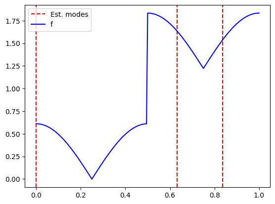
(a) Graph of $f$ and estimated modes

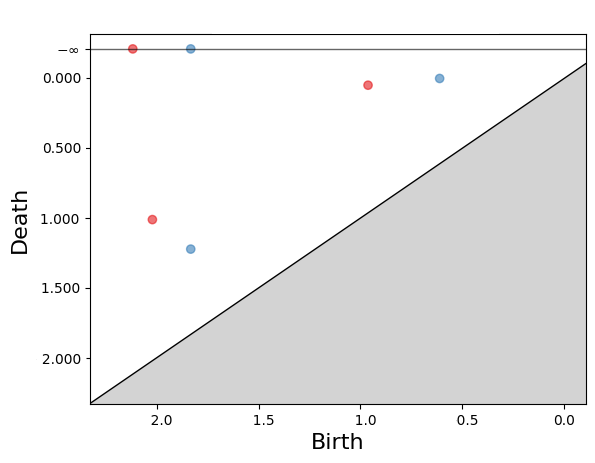
(b) True and estimated persistence diagram

Figure 8: 1D numerical illustration, example 1.

Example 2.1. Here, we consider the 2D density given by the normalization of $f$ define by,

$$f(x,y)= 2\left(\frac{1}{20}-\left\|(x,y)-(1/4,1/4)\right\|_{2}^{2}\right)_{+}+4\left(\frac{1}{20}-\left\|(x,y)-(3/4,3/4)\right\|_{2}^{2}\right)_{+}$$

$$+\left(\frac{1}{16}-\left\|(x,y)-(3/4,1/4)\right\|_{2}^{2}\right)_{+}+\left(\frac{1}{16}-\left\|(x,y)-(1/4,3/4)\right\|_{2}^{2}\right)_{+}$$

if $1/4\leq y\leq 3/4$ and $1/4-(y-1/4)(y_{3}/4)\leq x\leq 3/4+(y-1/4)(y-3/4)$ and else $f(x,y)=0$.

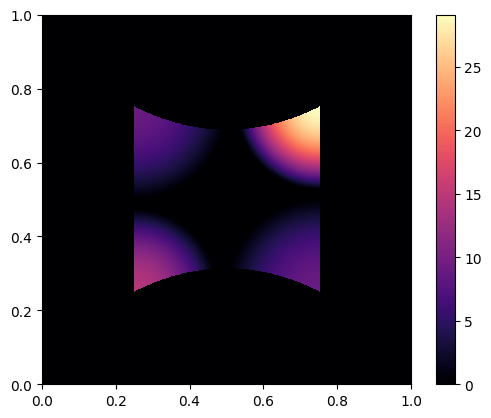
Figure 9: Graph of $f$

Again, this function is interesting as it is not continuous in any neighborhood of the modes, but only in a small half cone containing the modes. Additionally, one can check that this function in $S_{d}(L,1/2,\mu,R_{\mu},C,h_{0},l)$ for $\mu\leq 1/2$ and some $L>0$, $R_{\mu}>0$, $C>0$, $h_{0}>0$. We sample $n=10000$ points according to $f$, and choose the parameters $\mu=1/2$ and $h=(\log(n)/n)^{1/3}/6$.

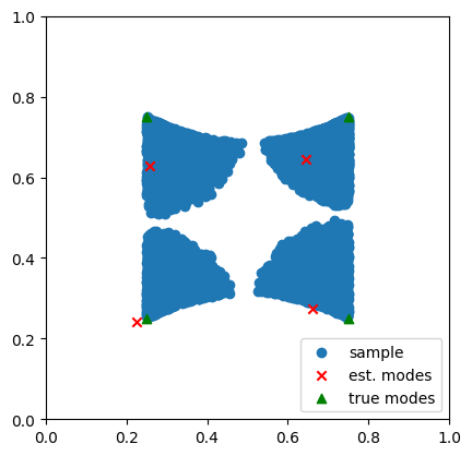
(a) Sampled points, true and estimated modes

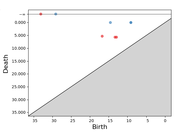
(b) True and estimated persistence diagrams

Figure 10: 2D numerical illustration, example 2.1.

Example 2.2. We propose another 2D example by considering the normalization of $f$ defined by,

$$f(x,y)=\frac{1}{2}\left(1/8-\left\|(x,y)-(1/4,1/2)\right\|_{2}\right)_{+}$$

if $|x-1/4|+|y-1/4|\leq 1/4$ or $|x-1/4|+|y-3/4|\leq 1/4$,

$$f(x,y)=\left(1/8-\left\|(x,y)-(3/4,1/2)\right\|_{2}\right)_{+}$$

if $|x-3/4|+|y-3/4|\leq 1/4$ or $|x-3/4|+|y-1/4|\leq 1/4$, and $f(x,y)=0$ else.

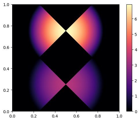
Figure 11: Graph of $f$

In all neighborhood of the modes $f$ is discontinuous. But again, one can check that this function belongs to $S_{d}(L,1/2,\mu,R_{\mu},C,h_{0})$ for $\mu<\sqrt{2}/2$ and some $L>0$, $R_{\mu}>0$, $C>0$, $h_{0}>0$. This example is interesting as, for each mode, capturing the connectivity of the two "half cones" intersecting at the mode can be difficult, as illustrated in Figure 7. We sample $n=30000$ points according to $f$, and choose the parameters $\mu=1/2$ and $h=(\log(n)/n)^{1/3}/4$.

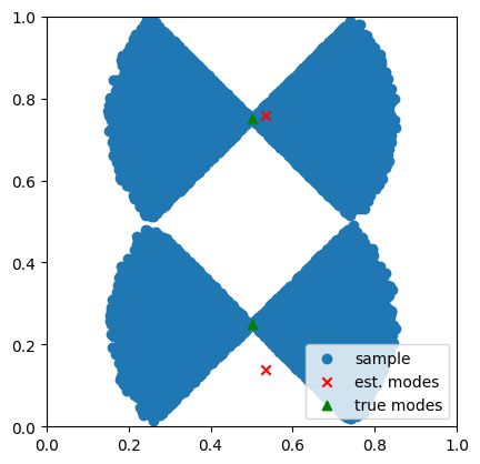
(a) Sampled points, true and estimated modes

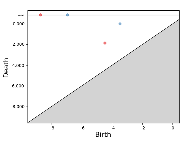
(b) True and estimated persistence diagrams

Figure 12: 2D numerical illustration, example 2.2.

5 Discussion

Exploiting the link between modes and persistence, we propose an estimator that permits to infer consistently the number of modes, their location and associated local maxima. We lead a rigorous study of the convergence properties of this estimator, showing that it achieves minimax rates over large classes of densities. In contrast to existing work, our approach involves distinct density assumptions. While we impose a stronger global regularity assumption, we concurrently relax requirements around modes. Notably, we do not presume continuity in the neighborhood of modes, but only in small half cones containing modes. This provides new insights and perspectives on multiple modes inference.

Along the way, we also extend the approach and results of Henneuse (2024) for $H_{0}$-persistence diagram estimation, for the density model. We believe that these results are interesting by themselves as they extend the current scope on persistent homology inference for density that mainly remained limited to regular density. These results show some strong robustness to discontinuity of $H_{0}-$persistence diagram estimation. We currently work on generalization for higher order homology.

Another point of interest is the adaptivity of such methods. Here, the proposed estimators depend on the regularity parameters $\alpha$ and the curvature measure of the discontinuity set $\mu$. While the dependence in $\alpha$ can be handled via standard methods, such as Lepski’s method (as done in Henneuse (2024)), overcoming the dependence in $\mu$ is less straightforward. Exploring methodologies to develop adaptive procedures to $\mu$ requires further dedicated research.

Appendix A Proof of Lemma 4

This section is dedicated to the proof of Lemma 4.

Proof of Lemma 4.

The first part of the claim is Theorem 12 of Kim et al. (2020). A standard technics to construct deformation retract in differential topology is to exploit the flow coming from a smooth underlying vector field. In Kim et al. (2020), their idea is to use the vector field defined on $B_{2}(K,r)\setminus K$, by $W(x)=-\nabla_{K}(x)$. But this vector field is not continuous. To overcome this issue, they construct a locally finite covering $(U_{x_{i}})_{i\in\mathbb{N}}$ of $B_{2}(K,r)\setminus K$ and an associated partition of the unity $(\rho_{i})_{{i\in\mathbb{N}}}$, such that $\overline{W}(x)=\sum_{i\in\mathbb{N}}\rho_{i}(x)w(x_{i})$ share the same dynamic as $W$. More precisely, they show that $\overline{W}$ induced a smooth flow $C$ that can be extended on $B_{2}(K,r)\times[0,+\infty[$ such that for all $x\in B_{2}(K,r)$, for all $t\geq 2r/\mu^{2}$, $C(x,t)=C(x,2r/\mu^{2})\in K$. We make an additional remark, denotes $d_{C}$ the arc length distance along $C$, as $||W||\leq 1$, we have,

$$d_{C}(x,C(x,2r/\mu^{2})) =\int_{0}^{2r/\mu^{2}}\left|\frac{\partial}{\partial t}C(x,t)\right|dt$$

$$\leq\int_{0}^{2r/\mu^{2}}||W(C(x,t)||_{2}dt$$

$$\leq 2r/\mu^{2}$$ (14)

Thus for all $t\in[°,+\infty[$, $||x-C(x,t)||_{2}\leq 2r/\mu^{2}$. Now taking, $F(x,s)=C(x,2rs/\mu^{2})$, provide a deformation retract of $B_{2}(K,r)$ onto $K$ and the associated retraction $R:x\mapsto F(x,1)$ verifies, $R(x)\in B_{2}(x,2r/\mu^{2})$ by (14). ∎

Appendix B Proof of Lemma 2

This Appendix is dedicated to the proof of Lemma 2.

Proof of Lemma 2.

Let $f\in S_{d}(L,\alpha,\mu,R_{\mu})$. Let $H\subset\mathcal{F}_{\lambda-2\sqrt{3M_{d,L,R_{\mu}}}N_{h}h^{\alpha}}^{c}\cap C_{h}$ and $H^{{}^{\prime}}\subset\mathcal{F}_{\lambda+2\sqrt{3M_{d,L,R_{\mu}}}N_{h}+h^{\alpha}}\cap C_{h}$. Remark that $f|_{H^{{}^{\prime}}}<\lambda-2\sqrt{3M_{d,L,R_{\mu}}}N_{h}h^{\alpha}$ and $f|_{H}\geq\lambda+2\sqrt{3M_{d,L,R_{\mu}}}N_{h}h^{\alpha}$. Thus,

$$\mathbb{P}(X_{1}\in H|N_{h})<(\lambda-2\sqrt{3M_{d,L,R_{\mu}}}N_{h}h^{\alpha})h^{d}$$

and

$$\mathbb{P}(X_{1}\in H^{{}^{\prime}}|N_{h})\geq(\lambda+2\sqrt{3M_{d,L,R_{\mu}}}N_{h}h^{\alpha})h^{d}.$$

As, supposing $N_{h}$ known, $|X\cap H|$ is $(n,\mathbb{P}(X_{1}\in H|N_{h})-$binomial and $|X\cap H^{{}^{\prime}}|$ is $(n,\mathbb{P}(X_{1}\in H^{{}^{\prime}}|N_{h})-$binomial we have that,

$$\mathbb{E}\left[\frac{|X\cap H|}{nh^{d}}|N_{h}\right]=\frac{\mathbb{P}(X_{1}\in H|N_{h})}{h^{d}}<\lambda-2\sqrt{3M_{d,L,R_{\mu}}}N_{h}h^{\alpha}$$

and

$$\mathbb{E}\left[\frac{|X\cap H^{{}^{\prime}}|}{nh^{d}}|N_{h}\right]=\frac{\mathbb{P}(X_{1}\in H^{{}^{\prime}}|N_{h})}{h^{d}}\geq\lambda+2\sqrt{3M_{d,L,R_{\mu}}}N_{h}h^{\alpha}.$$

Then, by the choice made for $h$,

$$\frac{|X\cap H|}{nh^{d}} =\mathbb{E}\left[\frac{|X\cap H|}{nh^{d}}|N_{h}\right]+\frac{|X\cap H|}{nh^{d}}-\mathbb{E}\left[\frac{|X\cap H|}{nh^{d}}|N_{h}\right]$$

$$=\mathbb{E}\left[\frac{|X\cap H|}{nh^{d}}|N_{h}\right]+\frac{|X\cap H|}{nh^{d}}-\mathbb{E}\left[\frac{|X\cap H|}{nh^{d}}\right]-\mathbb{E}\left[\frac{|X\cap H|}{nh^{d}}-\mathbb{E}\left[\frac{|X\cap H|}{nh^{d}}\right]|N_{h}\right]$$

$$\leq\mathbb{E}\left[\frac{|X\cap H|}{nh^{d}}|N_{h}\right]+2\sqrt{3M_{d,L,R_{\mu}}}N_{h}\sqrt{\frac{\log\left(1/h^{d}\right)}{nh^{d}}}<\lambda$$

and similarly,

$$\frac{|X\cap H^{{}^{\prime}}|}{nh^{d}}\geq\mathbb{E}\left[\frac{|X\cap H^{{}^{\prime}}|}{nh^{d}}|N_{h}\right]-2\sqrt{3M_{d,L,R_{\mu}}}N_{h}\sqrt{\frac{\log\left(1/h^{d}\right)}{nh^{d}}}>\lambda$$

and the proof is complete. ∎

Appendix C Proof of Lemma 1

This Appendix is dedicated to the proof of Lemma 1.

Proof of Lemma 1.

Let $i\in\{1,...,l\}$. First suppose that $d=1$, in this case, $\partial M_{i}$ is the union of two singletons $\{x_{1}\}\cup\{x_{2}\}$. The medial axis is equal here to the set of critical points, which is simply given by $\{(x_{1}+x_{2})/2\}$. Thus, by Assumption A3, we have $|x_{1}-x_{2}|>2R_{\mu}$. Let $x\in M_{i}$, by Assumption A1,

$$2R_{\mu}(f(x)-L)\leq\int_{x_{1}}^{x_{2}}f(u)du.$$

Hence, as $f$ is a density,

$$\int_{x_{1}}^{x_{2}}f(u)du\leq 1$$

and

$$f(x)\leq\frac{1}{2R_{\mu}}+L:=M_{1,L,R_{\mu}}.$$

Now, for $d>1$, if the $\mu-$medial axis of $\partial M_{i}$ intersected with $M_{i}$ is empty, then $M_{i}^{c}$ has infinite $\mu-$reach. By Theorem 12 of Kim et al. (2020), this implies that for any $r>0$, $\left(M_{i}^{c}\right)^{r}$ is homotopy equivalent to $M_{i}^{c}$. For $r>\sqrt{d}$, $\left(M_{i}^{c}\right)^{r}=[0,1]^{d}$, and thus has trivial $s-$homotopy groups for $s>0$ but $M_{i}^{c}$ contains a non-trivial $d-1$ cycles represented by $\partial M_{i}$, which gives a contradiction. Consequently, $M_{i}$ contains a point $x_{1}$ belonging to the $\mu-$medial axis of $\partial M_{i}$. By Assumption A3, $B_{2}(x_{1},R_{\mu}/2)$ is contained into $M_{i}$. Thus, Assumption A1 ensures that,

$$V_{d}(R_{\mu}/2))(f(x_{1})-L(2R_{\mu})^{\alpha})\leq\int_{B_{2}(x_{1},R_{\mu}/2)}f(u)du$$

with $V_{d}(R_{\mu}/2))$ the volume of the $d-$dimensional Euclidean ball of radius $R_{\mu}/2$. As $f$ is a density,

$$\int_{B_{2}(x_{1},R_{\mu}/2)}f(u)du\leq 1$$

and hence,

$$f(x_{1})\leq\frac{1}{V_{d}(R_{\mu}/2))}+LR_{\mu}^{\alpha}.$$

Now, let $x\in M_{i}$, we have $||x-x_{1}||\leq\sqrt{d}$, using Assumption A1 again, it follows that,

$$f(x)\leq f(x_{1})+Ld^{\alpha/2}\leq\frac{1}{V_{d}(R_{\mu}))}+L(R_{\mu}^{\alpha}+d^{\alpha/2}):=M_{d,L,R_{\mu}}.$$

To conclude, it suffices to remark that Assumption A2 ensures that,

$$\sup\limits_{x\in\bigcup\limits_{i=1}^{l}M_{i}}f(x)=\sup\limits_{x\in[0,1]^{d}}f(x)$$

and thus for all $x\in[0,1]^{d}$,

$$f(x)\leq M_{d,L,R_{\mu}}.$$

∎

Appendix D Proof for the $q-$tameness

We here prove the claim that the persistence modules we introduced estimator are $q-$tame and consequently their persistence diagram are well-defined.

Proposition 4.

Let $f\in S_{d}(L,\alpha,\mu,R_{\mu})$ then $f$ is $q$-tame.

Proof.

Let $s\in\mathbb{N}$ and $\mathbb{V}_{0,f}$ the persistence module (for the $0-$th homology) associated to the sublevel filtration, $\mathcal{F}$ and for fixed levels $\lambda>\lambda^{{}^{\prime}}$ let denote $v_{\lambda}^{\lambda^{{}^{\prime}}}$ the associated map. Let $\lambda\in\mathbb{R}$ and $h<\frac{R_{\mu}}{2}$. By Proposition 2,

$$v_{\lambda}^{\lambda-L\left(\sqrt{d}(2+2/\mu^{2})\right)^{\alpha}h^{\alpha}}=\phi_{\lambda}\circ\tilde{i}_{\lambda}\text{, with }\tilde{i}_{\lambda}:H_{0}\left(\mathcal{F}_{\lambda}\right)\rightarrow H_{0}\left(\mathcal{F}_{\lambda}^{h}\right)\text{ induced by inclusion.}$$

By assumption A1 and A2, $\mathcal{F}_{\lambda}$ is compact. As $[0,1]^{d}$ is triangulable, $\mathcal{F}_{\lambda}$ is covered by finitely many cells of the triangulation, and so there is a finite simplicial complex $K$ such that $\overline{\mathcal{F}_{\lambda}}\subset K\subset\mathcal{F}_{\lambda}^{h}$. Consequently, $\tilde{i}_{\lambda}$ factors through the finite dimensional space $H_{0}(K)$ and is then of finite rank by Theorem 1.1 of Crawley-Boevey (2012).

Thus, $v_{\lambda}^{\lambda-L\left(\sqrt{d}(2+2/\mu^{2})\right)^{\alpha}h^{\alpha}}$ is of finite rank for all $0<h<\frac{R_{\mu}}{2}$. As for any $\lambda>\lambda^{{}^{\prime}}>\lambda^{{}^{\prime\prime}}$, $v_{\lambda}^{\lambda^{{}^{\prime\prime}}}=v_{\lambda^{{}^{\prime}}}^{\lambda^{{}^{\prime\prime}}}\circ v_{\lambda}^{\lambda^{{}^{\prime}}}$ we then have that $v_{\lambda}^{\lambda^{{}^{\prime}}}$ is of finite rank for all $\lambda>\lambda^{{}^{\prime}}$. Hence, $f$ is $q$-tame. ∎

Lemma 6.

Let $f:[0,1]^{d}\rightarrow\mathbb{R}$ then, for all $s\in\mathbb{N}$ $\widehat{\mathbb{V}}_{0,f}$ is $q$-tame.

Proof.

Let $h>0$ and $\lambda\in\mathbb{R}$. By construction $\widehat{\mathcal{F}}_{\lambda}$ is a union of cubes of the regular grid $G(h)$, thus $H_{0}(\widehat{\mathcal{F}}_{\lambda})$ is finite dimensional. Thus $\widehat{\mathbb{V}}_{0,f}$ is $q$-tame by Theorem 1.1 of Crawley-Boevey (2012). ∎

References

- Abraham et al. (2003) Christophe Abraham, Gérard Biau, and Benoît Cadre. Simple estimation of the mode of a multivariate density. Canadian Journal of Statistics, 31(1):23–34, 2003. doi: 10.2307/3315901.
- Abraham et al. (2004) Christophe Abraham, Gérard Biau, and Benoît Cadre. On the asymptotic properties of a simple estimate of the mode. ESAIM: PS, 8:1–11, 2004. doi: 10.1051/ps:2003015.
- Ameijeiras-Alonso et al. (2019) Jose Ameijeiras-Alonso, Rosa M. Crujeiras, and Alberto Rodríguez-Casal. Mode testing, critical bandwidth and excess mass. TEST, 28:900–919, 2019. doi: 10.1007/s11749-018-0611-5.
- Arias-Castro et al. (2016) Ery Arias-Castro, David Mason, and Bruno Pelletier. On the estimation of the gradient lines of a density and the consistency of the mean-shift algorithm. Journal of Machine Learning Research, 17(43):1–28, 2016.
- Arias-Castro et al. (2022) Ery Arias-Castro, Wanli Qiao, and Lin Zheng. Estimation of the global mode of a density: Minimaxity, adaptation, and computational complexity. Electronic Journal of Statistics, 16(1):2774 – 2795, 2022. doi: 10.1214/21-EJS1972.
- Barannikov (1994) Serguei Barannikov. The framed morse complex and its invariants. Adv. Soviet Math., 21:93–115, 1994.
- Bauer et al. (2014) Ulrich Bauer, Axel Munk, Hannes Sieling, and Max Wardetzky. Persistent homology meets statistical inference - a case study: Detecting modes of one-dimensional signals. 2014.
- Bobrowski et al. (2017) Omer Bobrowski, Sayan Mukherjee, and Jonathan E. Taylor. Topological consistency via kernel estimation. Bernoulli, 23(1):288 – 328, 2017. doi: 10.3150/15-BEJ744.
- Bubenik et al. (2009) Peter Bubenik, Gunnar Carlsson, Peter Kim, and Zhiming Luo. Statistical topology via morse theory persistence and nonparametric estimation. Contemporary Mathematics, 516:75–92, 2009. doi: 10.1090/conm/516/10167.
- Burman and Polonik (2009) Prabir Burman and Wolfgang Polonik. Multivariate mode hunting: Data analytic tools with measures of significance. Journal of Multivariate Analysis, 100(6):1198–1218, 2009. doi: 10.1016/j.jmva.2008.10.015.
- Carreira-Perpinan (2007) Miguel Carreira-Perpinan. Gaussian mean-shift is an em algorithm. IEEE Transactions on Pattern Analysis and Machine Intelligence, 29(5):767–776, 2007. doi: 10.1109/TPAMI.2007.1057.
- Carreira-Perpinan and Williams (2003) Miguel Carreira-Perpinan and Christopher Williams. On the number of modes of a gaussian mixture. In Scale Space Methods in Computer Vision, pages 625–640. Springer Berlin Heidelberg, 2003. doi: 10.1007/3-540-44935-3_44.
- Chacón (2012) José Chacón. Clusters and water flows: a novel approach to modal clustering through morse theory. 2012.
- Chacón (2020) José Chacón. The modal age of statistics. International Statistical Review, 88, 2020. doi: 10.1111/insr.12340.
- Chazal et al. (2009) Frédéric Chazal, David Cohen-Steiner, Marc Glisse, Leonidas J. Guibas, and Steve Y. Oudot. Proximity of persistence modules and their diagrams. In Proceedings of the Twenty-Fifth Annual Symposium on Computational Geometry, SCG ’09, page 237–246, 2009. doi: 10.1145/1542362.1542407.
- Chazal et al. (2016) Frédéric Chazal, Steve Oudot, Marc Glisse, and Vin de Silva. The Structure and Stability of Persistence Modules. SpringerBriefs in Mathematics. Springer Verlag, 2016. doi: 10.1007/978-3-319-42545-0.
- Chazal and Michel (2021) Frédéric Chazal and Bertrand Michel. An introduction to topological data analysis: fundamental and practical aspects for data scientists, 2021.
- Chazal et al. (2006) Frédéric Chazal, David Cohen-Steiner, and André Lieutier. A sampling theory for compact sets in euclidean space. Discrete & Computational Geometry, 41:461–479, 2006. doi: 10.1007/s00454-009-9144-8.
- Chazal et al. (2007) Frédéric Chazal, David Cohen-Steiner, André Lieutier, and Boris Thibert. Shape smoothing using double offset. Proceedings - SPM 2007: ACM Symposium on Solid and Physical Modeling, 2007. doi: 10.1145/1236246.1236273.
- Chazal et al. (2011) Frédéric Chazal, Leonidas Guibas, Steve Oudot, and Primoz Skraba. Persistence-based clustering in riemannian manifolds. Journal of the ACM, 60, 2011. doi: 10.1145/2535927.
- Cheng and Hall (1998) Ming-Yen Cheng and Peter Hall. Calibrating the excess mass and dip tests of modality. Journal of the Royal Statistical Society. Series B (Statistical Methodology), 60(3):579–589, 1998.
- Cheng (1995) Yizong Cheng. Mean shift, mode seeking, and clustering. IEEE Transactions on Pattern Analysis and Machine Intelligence, 17(8):790–799, 1995. doi: 10.1109/34.400568.
- Chernoff (1964) Herbert Chernoff. Estimation of the mode. Annals of the Institute of Statistical Mathematics, 16, 1964.
- Cohen-Steiner et al. (2005) David Cohen-Steiner, Herbert Edelsbrunner, and John Harer. Stability of persistence diagrams. Discrete and Computational Geometry - DCG, 37:263–271, 2005. doi: 10.1007/s00454-006-1276-5.
- Comaniciu and Meer (2002) Dorin Comaniciu and Peter Meer. Mean shift: a robust approach toward feature space analysis. IEEE Transactions on Pattern Analysis and Machine Intelligence, 24(5):603–619, 2002. doi: 10.1109/34.1000236.
- Crawley-Boevey (2012) William Crawley-Boevey. Decomposition of pointwise finite-dimensional persistence modules, 2012.
- Dasgupta and Kpotufe (2014) Sanjoy Dasgupta and Samory Kpotufe. Optimal rates for k-nn density and mode estimation. In Advances in Neural Information Processing Systems, volume 27. Curran Associates, Inc., 2014.
- Devroye (1979) Luc Devroye. Recursive estimation of the mode of a multivariate density. Canadian Journal of Statistics, 7(2):159–167, 1979. doi: 10.2307/3315115.
- Donoho and Liu (1991) David Donoho and Richard Liu. Geometrizing Rates of Convergence, III. The Annals of Statistics, 19(2):668 – 701, 1991. doi: 10.1214/aos/1176348115.
- Duong et al. (2008) Tarn Duong, Arianna Cowling, Inge Koch, and Matt Wand. Feature significance for multivariate kernel density estimation. Computational Statistics & Data Analysis, 52:4225–4242, 2008. doi: 10.1016/j.csda.2008.02.035.
- Eddy (1980) William Eddy. Optimum Kernel Estimators of the Mode. The Annals of Statistics, 8(4):870 – 882, 1980. doi: 10.1214/aos/1176345080.
- Federer (1959) Herbert Federer. Curvature measures. Trans. Amer. Math. Soc, 1959.
- Fisher and Marron (2001) Nick Fisher and Steve Marron. Mode testing via the excess mass estimate. Biometrika, 88(2):499–517, 2001.
- Fukunaga and Hostetler (1975) Keinosuke Fukunaga and Larry Hostetler. The estimation of the gradient of a density function, with applications in pattern recognition. IEEE Transactions on Information Theory, 21(1):32–40, 1975. doi: 10.1109/TIT.1975.1055330.
- Genovese et al. (2015) Christopher Genovese, Marco Perone-Pacifico, Isabella Verdinelli, and Larry Wasserman. Non-Parametric Inference for Density Modes. Journal of the Royal Statistical Society Series B: Statistical Methodology, 78(1):99–126, 2015.
- Hall and York (2001) Peter Hall and Matthew York. On the calibration of silverman’s test for multimodality. Statistica Sinica, 11(2):515–536, 2001.
- Hartigan and Hartigan (1985) John Hartigan and P. M. Hartigan. The Dip Test of Unimodality. The Annals of Statistics, 13(1):70 – 84, 1985. doi: 10.1214/aos/1176346577.
- Hatcher (2000) Allen Hatcher. Algebraic topology. Cambridge Univ. Press, Cambridge, 2000.
- Henneuse (2024) Hugo Henneuse. Persistence diagram estimation of multivariate piecewise hölder-continuous signals. 2024.
- Jiang and Kpotufe (2017) Heinrich Jiang and Samory Kpotufe. Modal-set estimation with an application to clustering. In Proceedings of the 20th International Conference on Artificial Intelligence and Statistics, volume 54 of Proceedings of Machine Learning Research, pages 1197–1206. PMLR, 2017.
- Kim et al. (2020) Jisu Kim, Jaehyeok Shin, Frédéric Chazal, Alessandro Rinaldo, and Larry Wasserman. Homotopy reconstruction via the cech complex and the vietoris-rips complex, 2020.
- Klemelä (2005) Jussi Klemelä. Adaptive estimation of the mode of a multivariate density. Journal of Nonparametric Statistics, 17(1):83–105, 2005. doi: 10.1080/10485250410001723151.
- Konakov (1974) Valentin Konakov. On the asymptotic normality of the mode of multidimensional distributions. Theory of Probability & Its Applications, 18(4):794–799, 1974. doi: 10.1137/1118104.
- Lepski (1992) Oleg Lepski. Asymptotically minimax adaptive estimation. i: Upper bounds. optimally adaptive estimates. Theory of Probability & Its Applications, 36(4):682–697, 1992. doi: 10.1137/113608.
- Li et al. (2007) Jia Li, Surajit Ray, and Bruce Lindsay. A nonparametric statistical approach to clustering via mode identification. Journal of Machine Learning Research, 8:1687–1723, 2007.
- Minnotte (1997) Michael Minnotte. Nonparametric testing of the existence of modes. The Annals of Statistics, 25(4):1646 – 1660, 1997. doi: 10.1214/aos/1031594735.
- Mokkadem and Pelletier (2003) Abdelkader Mokkadem and Mariane Pelletier. The law of the iterated logarithm for the multivariate kernel mode estimator. Esaim: Probability and Statistics, 7:1–21, 2003.
- Parzen (1962) Emanuel Parzen. On Estimation of a Probability Density Function and Mode. The Annals of Mathematical Statistics, 33(3):1065 – 1076, 1962.
- Romano (1988) Joseph Romano. On Weak Convergence and Optimality of Kernel Density Estimates of the Mode. The Annals of Statistics, 16(2):629 – 647, 1988. doi: 10.1214/aos/1176350824.
- Samanta (1973) Mrityunjay Samanta. Nonparametric estimation of the mode of a multivariate density. South African Statistical Journal, 7:109–117, 1973.
- Silverman (1981) Bernard Silverman. Using kernel density estimates to investigate multimodality. Journal of the Royal Statistical Society: Series B (Methodological), 43(1):97–99, 1981.
- Tsybakov (1990) Alexandre Tsybakov. Recursive estimation of the mode of a multivariate distribution. Problemy Peredachi Informatsii, 26:38–45, 1990.
- Tsybakov (2008) Alexandre Tsybakov. Introduction to Nonparametric Estimation. Springer Publishing Company, Incorporated, 2008.
- Vieu (1996) Phillipe Vieu. A note on density mode estimation. Statist. Probab. Lett., 26:297–307, 1996. doi: 10.1016/0167-7152(95)00024-0.