Primordial black holes in SB SUSY Gauss-Bonnet inflation

Abstract

Here, we explore the formation of primordial black holes (PBHs) within a scalar field inflationary model coupled to the Gauss-Bonnet (GB) term, incorporating low-scale spontaneously broken supersymmetric (SB SUSY) potential. The coupling function amplifies the curvature perturbations, consequently leading to the formation of PBHs and the production of detectable secondary gravitational waves (GWs). Through the adjustment of model parameters, the inflaton can be decelerated during the ultra-slow-roll (USR) phase, thereby augmenting curvature perturbations. Swampland criteria are also investigated. Our computations forecast the formation of PBHs with masses on the order of ${\cal O}(10)M_{\odot}$, aligning with observational data from LIGO-Virgo and PBHs with masses ${\cal O}(10^{-6})M_{\odot}$, offering potential explanation for ultrashort-timescale microlensing events recorded in OGLE data. Additionally, our proposed mechanism can generate PBHs with masses around ${\cal O}(10^{-13})M_{\odot}$, constituting roughly 99$\%$ of the dark matter. The density parameter of produced GWs ($\Omega_{\rm GW_{0}}$) intersects with the sensitivity curves of GW detectors. Two cases of our model fall within the nano-Hz regime. One of these satisfies the $\Omega_{\rm{GW}}(f)\sim f^{5-\gamma}$ fit, with the derived $\gamma=3.51$ matching the NANOGrav 15-year data.

I Introduction

The initial concept of generating PBHs from curvature perturbations was introduced by Zel’dovich and Novikov zeldovich:1967 . Subsequent investigations have revealed that low-mass PBHs underwent complete evaporation in the early universe as a result of quantum effects, whereas more massive PBHs may remain until the present epoch Hawking:1974 ; Hawking:1976 ; Hawking:1971 ; Page:1976 ; carr:1975 ; carr:1974 . PBHs are strong candidate for either all or a fraction of the dark matter content Nojiri:2017 ; Olmo:2011 ; Capozziello:2011 ; Nojiri:2011 ; Cruz-Dombriz:2012 ; Chapline:1975 ; Ivanov:1994 ; Polnarev:1985 ; Teimoori-b:2021 ; Solbi-b:2021 ; Rezazadeh:2021 ; Solbi-a:2021 ; YCai:2021 ; YCai:2023 ; AChakraborty:2022 ; GDomenech:2023 ; TPapanikolaou:2022 ; TPapanikolaou:2023a ; TPapanikolaou:2023b ; SChoudhury:2014 . The detection of GWs from a binary black hole merger by the LIGO-Virgo collaboration has drawn PBHs into focus Abbott:2016 ; Abbott:2016-a ; Abbott:2016-b ; Abbott:2017-a ; Abbott:2017-b ; Abbott:2017-c ; Abbott:2017 ; Abbott:2019 . PBHs with mass scale of ${\cal O}(10)M_{\odot}$ could be the source of GWs observed by LIGO-Virgo. Also, PBHs with masses around ${\cal O}(10^{-5})M_{\odot}$ could offer an explanation for the ultrashort-timescale microlensing events observed in OGLE data OGLE . Furthermore, PBHs within the mass range ${\cal O}(10^{-16}-10^{-11})M_{\odot}$, could comprise the entirety of the dark matter content Gould:1992 ; Alcock:2001 ; Teimoori:2021 ; Heydari:2021 ; Heydari:2024 ; Heydari:2022 ; Heydari:2023a ; Heydari:2023b ; Solbi:2024 ; Dalcanton:1994 ; Laha:2020 ; Ali-Haimoud:2017 ; Sato-Polito:2019 ; Wang:2018 ; Jacobs:2015 .

Generation of PBHs in the radiation-dominated (RD) era requires a considerable amplitude of primordial curvature perturbations during the inflationary epoch. As the perturbed superhorizon scales, characterized by large amplitudes, become subhorizon during the RD era, gravitational collapse of the resulting overdense regions leads to form PBHs.

The formation of PBHs requires the scalar power spectrum to increase to the order of $\mathcal{O}(10^{-2})$ at small scales. However, cosmic microwave background (CMB) measurements have disclosed that the amplitude of the scalar power spectrum at the pivot scale $k_{*}=0.05~{}\mathrm{Mpc}^{-1}$ should be $2.1\times 10^{-9}$ akrami:2020 . Consequently, the scalar power spectrum would need to be enhanced by seven orders of magnitude at small scales to be suitable to form PBHs Mishra:2020 ; Fu:2019 ; Kawai:2021 ; Dalianis:2019 ; mahbub:2020 ; Kawaguchia:2023 ; Villanueva-Domingo:2021 ; Ashrafzadeh:2024 ; Gao:2021 ; Lin:2020 ; Kamenshchik:2019 ; Zhang:2022 ; SChoudhury:2023 .

The re-entry of the amplified scales to the horizon during the RD era may give rise to the generation of secondary GWs concurrently with the formation of PBHs. Consequently, identification of the secondary GWs signals presents a novel method for indirectly detecting PBHs Bhattacharya:2023 ; GDomenech:2021a ; GDomenech:2021b ; GDomenech:2024 ; SMittal:2022 ; MRGangopadhyay:2023b ; GBhattacharya:2023 . In other words, the collapse of amplified curvature perturbations upon horizon re-entry generates significant metric perturbations. At the second order, scalar and tensor perturbations can interact, unlike the linear level. As a result, second-order scalar metric perturbations can produce GWs background BartoloPRL:2019 ; BartoloPRD:2019 ; CaiPRL:2019 ; Fumagalli:2021 ; CaiJCAP:2019 ; Wang:2019 ; CaiPRD:2019 . Since the NANOGrav signal remains unconfirmed, it is difficult to propose plausible mechanisms for its origin. In this regard, the NANOGrav pulsar timing array team has recently unveiled background GWs within 15 years of data Agazie1:2023 ; Agazie2:2023 ; Agazie3:2023 ; Agazie4:2023 .

One widely utilized strategy for amplifying the scalar power spectrum involves initiating a brief USR phase. Within this phase, the inflaton undergoes effective deceleration, consequently resulting in a substantial increase in curvature perturbations Ragavendra:2023 . The creation of the USR region is imperative for PBHs production during inflation and can be achieved through various means. Under slow-roll conditions, the scalar power spectrum does not increase enough to PBHs formation. Conversely, during the USR phase, decrease in the inflaton velocity provides sufficient time for amplification of primordial curvature perturbations, which can subsequently result in PBH formation after re-entering the horizon. This process is attainable both within the standard model of inflation and the frameworks of modified gravity. In the standard single-field inflationary model, when the potential has an inflection point, there is a notable reduction in the velocity of the inflaton in the vicinity of this point. Consequently, during the USR phase, the scalar power spectrum can be augmented to generate suitable overdense regions conducive to PBH formation Mishra:2020 ; Dalianis:2019 ; mahbub:2020 . Furthermore, within the framework of modified gravity, the conditions for entering the USR phase can be established through the selection of an appropriate coupling function and fine-tuning of model parameters Fu:2019 ; Kawai:2021 ; Kawaguchia:2023 ; Villanueva-Domingo:2021 ; Gao:2021 ; Lin:2020 ; Kamenshchik:2019 ; Zhang:2022 ; SChoudhury:2023 . For instance, in the non-minimal and non-canonical models, the production of PBHs has been explained by employing suitable coupling functions Fu:2019 ; Gao:2021 ; Lin:2020 ; Kamenshchik:2019 .

In recent years, numerous studies have focused on higher dimensional gravity to understand the low-energy limit of string theory. The examination of GB theory could offer a comprehensive framework for addressing conceptual issues related to gravity. The GB gravity, originally proposed by Lanczos Lanczos:1938 and subsequently proclaimed by David Lovelock Lovelock:1971 , represents a significant higher-dimensional generalization of Einstein gravity Lanczos:1938 ; Lovelock:1971 ; RashidiNozari:2020 ; AziziNozari:2022 ; ShahraeiniNozari:2022 . In the GB theory, the order of the field equations does not exceed the second order, and the theory is free of ghost. Recently, numerous attempts have been made to derive black hole solutions. However, the first exact black hole solution in GB gravity was calculated by Boulware and Deser Boulware:1985 ; Myers:1988 . Subsequently, other researchers have explored exact black hole solutions with their thermodynamic properties Cho:2002 ; Sahabandu:2006 . Additionally, various black hole solutions with matter sources, extending the Boulware-Deser solution, have been discovered in HabibMazharimousavi:2009 ; Ghosh:2014 . In recent years, researchers have investigated the potential formation of PBHs within single field inflationary model coupled with the GB term. Through these works, they have been able to correct potentials such as the Higgs, natural and fractional power-law potential. The coupling function of modified gravity models with the GB term can enhance curvature perturbations at small scales, resulting in a notable abundance of PBHs and detectable secondary GWs Kawaguchia:2023 ; Kawai:2021 ; Ashrafzadeh:2024 ; Zhang:2022 .

In the next, the inflationary models are evaluated with swampland criteria. These criteria, derived from string theory, include the distance conjecture and the de Sitter conjecture. The validity of the de Sitter conjecture is not consistent with the slow-roll conditions in the standard inflation. Nevertheless, in modified inflationary models, both criteria can be satisfied Kehagias:2018 ; Garg:2019 ; Das:2019 ; Ooguri:2019 .

In this research, we aim to study the low-scale SB SUSY potential, which does not agree with the Planck observations in the standard model. Within the framework of modified gravity model with the GB term, we will examine the compatibility of the model with the latest observational constraints in addition to the swampland criteria thereto analyzing the PBHs production. Furthermore, we will investigate the GWs generated within the sensitivity range of the detectors. The structure of this paper is outlined as follows. Sect. II presents a summary of GB gravity. In Section III, we introduce the utilized technique to increase the amplitude of the curvature power spectrum at small scales. In Section IV, the fractional abundances and various masses of PBHs will be computed. In Section V, the energy spectra of GWs will be calculated. At the end, the summarized results are presented in Section VI.

II Summary of Gauss-Bonnet Inflationary Model

We regard the Einstein-Gauss-Bonnet action in the following Jiang:2013 ; Koh:2014 ; Guo:2010 ; Odintsov:2020 ; Gao:2020 ; AziziNozari:2022 ; ShahraeiniNozari:2022 ; RashidiNozari:2020 ; HAKhan:2022 ; MRGangopadhyay:2023a ; SDOdintsov:2020 ; SDOdintsov:2023 ; SNojiri:2023a ; EOPozdeeva:2020

$${\cal S}=\int{\rm d}^{4}x\sqrt{-g}\left[\frac{M_{\rm Pl}^{2}}{2}R-\frac{1}{2}g^{\mu\nu}\nabla_{\mu}\phi\nabla_{\nu}\phi-V(\phi)-\frac{\xi(\phi)}{2}R_{\rm GB}^{2}\right],$$ (1)

where $R$ is the Ricci scalar, $M_{\rm Pl}=(8\pi G)^{-1/2}$ is the reduced Planck mass, $R^{2}_{\rm GB}\equiv R_{\mu\nu\rho\sigma}R^{\mu\nu\rho\sigma}-4R_{\mu\nu}R^{\mu\nu}+R^{2}$ is the invariant scalar GB term and $\xi(\phi)$ is the coupling function between the scalar field $\phi$ and GB term. In this context, we examine a homogeneous and isotropic universe defined by a spatially flat Friedmann-Lemaître-Robertson-Walker (FLRW) metric.

The Friedmann equations and the equation of motion can be obtained by performing variations of the action (1) with respect to the metric $g^{\mu\nu}$ and the scalar field $\phi$, respectively, as follows Jiang:2013 ; Koh:2014 ; Guo:2010 ; Odintsov:2020 ; Gao:2020 ; HAKhan:2022 ; MRGangopadhyay:2023a ; SDOdintsov:2020 ; SDOdintsov:2023 ; SNojiri:2023a ; EOPozdeeva:2020

$$3{M_{\rm Pl}^{2}}H^{2}=\frac{1}{2}\dot{\phi}^{2}+V(\phi)+12\dot{\xi}H^{3},$$ (2)

$$-2{M_{\rm Pl}^{2}}\dot{H}=\dot{\phi}^{2}-4\ddot{\xi}H^{2}-4\dot{\xi}H\big{(}2\dot{H}-H^{2}\big{)},$$ (3)

$$\ddot{\phi}+3H\dot{\phi}+V_{,\phi}=-12\xi_{,\phi}H^{2}\big{(}\dot{H}+H^{2}\big{)},$$ (4)

where, $H\equiv\dot{a}/a$ is the Hubble parameter, $a$ is the scale factor, dot denotes the time derivative and the subscript $({,\phi})$ demonstrates derivative with respect to $\phi$.

In the GB gravity, the slow-roll parameters are determined as follows Jiang:2013 ; Koh:2014 ; Guo:2010 ; Odintsov:2020 ; Gao:2020

$$\epsilon_{1}\equiv\frac{-\dot{H}}{H^{2}},~{}~{}~{}\epsilon_{2}\equiv\frac{\ddot{\phi}}{H\dot{\phi}},~{}~{}~{}\delta_{1}\equiv 4\dot{\xi}H,~{}~{}~{}\delta_{2}\equiv\frac{\dot{\delta_{1}}}{H\delta_{1}}.$$ (5)

In order to attain a precise estimation of the curvature power spectrum, it is imperative to numerically solve the following Mukhanov-Sasaki (MS) equation

$$u_{k}^{\prime\prime}+\left(k^{2}-\frac{Z_{s}^{\prime\prime}}{Z_{s}}\right)u_{k}=0,$$ (6)

in which the prime means derivative versus the conformal time $\tau_{s}=\int\left({c_{s}}/{a}\right){\rm d}t$ and

$$u_{k}=Z_{s}\zeta_{k},\qquad Z_{s}=a\sqrt{2Q_{s}c_{s}},$$ (7)

with

$$Q_{s}=\frac{(8\dot{\phi}^{2}-48M_{\rm Pl}^{2}H^{2}+384H^{3}\xi_{,\phi}\dot{\phi})}{(M_{\rm Pl}^{2}H-6H^{2}\xi_{,\phi}\dot{\phi})^{2}}Q_{t}^{2}+12Q_{t},$$

$$c_{s}^{2}=\frac{1}{Q_{s}}\left[\frac{16}{a}\frac{{\rm d}}{{\rm d}t}\left(\frac{a~{}Q_{t}^{2}}{(M_{\rm Pl}^{2}H-6H^{2}\xi_{,\phi}\dot{\phi})}\right)-4c_{t}^{2}Q_{t}\right],$$ (8)

$$Q_{t}=\frac{1}{4}\left(M_{\rm Pl}^{2}-4H\xi_{,\phi}\dot{\phi}\right),\qquad$$

$$c_{t}^{2}=\frac{1}{4Q_{t}}\left(M_{\rm Pl}^{2}-4\xi_{,\phi\phi}\dot{\phi}^{2}-4\xi_{,\phi}\ddot{\phi}\right).$$ (9)

The requisite conditions to preclude the manifestation of ghost and Laplacian instabilities linked with scalar and tensor perturbations are outlined as follows

$$Q_{s}>0,\qquad c_{s}^{2}>0,\qquad Q_{t}>0,\qquad c_{t}^{2}>0.$$ (10)

Consequently, numerical solution of the MS equation (6) results in determination of the scalar power spectrum for each mode $u_{k}$ as follows

$${\cal P}_{s}(k)\equiv\frac{k^{3}}{2\pi^{2}}\left|\zeta_{k}(\tau_{s},{k})\right|^{2}.$$ (11)

In the regime of slow-roll conditions ($|\epsilon_{i}|\ll 1$ and $|\delta_{i}|\ll 1$), the background Eqs. (2)-(4) are simplified to

$$H^{2}\simeq\frac{V(\phi)}{3M_{\rm Pl}^{2}},$$ (12)

$$-2{M_{\rm Pl}^{2}}\dot{H}\simeq\dot{\phi}^{2}+4\dot{\xi}H^{3},$$ (13)

$$3H\dot{\phi}+V_{,\phi}\simeq-12\xi_{,\phi}H^{4}.$$ (14)

Also in the slow-roll approximation, the scalar power spectrum ${\cal P}_{s}(k)$ at the sound horizon crossing moment is given by Kawaguchia:2023 ; Felice:2011

$${\cal P}_{s}(k)\simeq\frac{H^{2}}{8\pi^{2}Q_{s}c_{s}^{3}}\biggr{|}_{c_{s}k=aH}.$$ (15)

The amplitude of scalar perturbations ${\cal P}_{s}(k)$ at the CMB scale $k_{*}=0.05~{}\rm Mpc^{-1}$ is ${\cal P}_{s}(k_{*})=2.1\times{10}^{-9}$, based on Planck 2018 data akrami:2020 . The scalar spectral index $n_{s}$ in the GB model in terms of the slow-roll parameters, Eq. (5), is derived as Jiang:2013

$$n_{s}-1\equiv\frac{{\rm d}\ln{\cal P}_{s}}{{\rm d}\ln k}\biggr{|}_{c_{s}k=aH}\simeq-2\epsilon_{1}-\frac{2\epsilon_{1}\epsilon_{2}-\delta_{1}\delta_{2}}{2\epsilon_{1}-\delta_{1}}.$$ (16)

After performing algebraic calculations and using the slow-roll approximation of the background Eqs. (12)-(14), the slow-roll parameters (5), can be expressed in terms of the potential and non-minimal coupling GB function as Jiang:2013 ; Koh:2014

$$\epsilon_{1} \simeq \epsilon_{V}+\frac{2}{3M_{\rm Pl}^{2}}V_{,\phi}\xi_{,\phi},\quad\qquad\qquad\qquad\qquad$$

$$\epsilon_{2} \simeq 4\epsilon_{V}-2\eta_{V}-\frac{4}{3M_{\rm Pl}^{2}}\frac{V}{V_{,\phi}}\left(\xi_{,\phi}V_{,\phi\phi}+V_{,\phi}\xi_{,\phi\phi}\right),\qquad\quad$$

$$\delta_{1} \simeq -\frac{4}{9M_{\rm Pl}^{4}}\xi_{,\phi}\left(3M_{\rm Pl}^{2}V_{,\phi}+\frac{4}{M_{\rm Pl}^{2}}V^{2}\xi_{,\phi}\right),\quad$$

$$\delta_{2} \simeq -\eta_{V}-\frac{8}{3M_{\rm Pl}^{2}}V\xi_{,\phi\phi}-V_{,\phi}\left(\frac{8}{3M_{\rm Pl}^{2}}\xi_{,\phi}+\frac{M_{\rm Pl}^{2}\xi_{,\phi\phi}}{V\xi_{,\phi}}\right).$$ (17)

In which $\epsilon_{V}\equiv\left({M_{\rm Pl}^{2}}/{2}\right)\left({V_{,\phi}}/{V}\right)^{2}$ and $\eta_{V}\equiv M_{\rm Pl}^{2}\left(V_{,\phi\phi}/V\right)$ are the potential slow-roll parameters in the standard inflation. Replacing the relations (17) into Eq. (16), one can get the scalar spectral index $n_{s}$ as

$$n_{s}-1\simeq-6\epsilon_{V}+2\eta_{V}+\frac{4}{3M_{\rm Pl}^{2}}V\xi_{,\phi}\left(\frac{V_{,\phi}}{V}+\frac{2\xi_{,\phi\phi}}{\xi_{,\phi}}\right).$$ (18)

Note that Eq. (18) for $\xi=0$ comes back to its equivalent result in the standard model. The value of the scalar spectral index, based on Planck 2018 TT, TE, EE + lowE + lensing + BK18 + BAO akrami:2020 , is $n_{s}=0.9649\pm 0.0042$ $(68\,\%\,\rm CL)$.
Identically, the tensor power spectrum is calculated using the subsequent MS equation Kawaguchia:2023 ; Felice:2011 ; Kawai:2021

$$u_{k}^{\prime\prime}+\left(k^{2}-\frac{Z_{t}^{\prime\prime}}{Z_{t}}\right)u_{k}=0,$$ (19)

where prime means derivative versus the conformal time $\tau_{t}=\int\left({c_{t}}/{a}\right){\rm d}t$. Also

$$u_{k}=Z_{t}\zeta_{t},\qquad Z_{t}=a\sqrt{2Q_{t}c_{t}}.$$ (20)

Solving the MS equation (19) yields the tensor power spectrum for each mode $u_{k}$ in the following manner

$${\cal P}_{t}(k)\equiv 4\frac{k^{3}}{2\pi^{2}}\left|\zeta_{t}(\tau_{t},{k})\right|^{2}.$$ (21)

Also in the slow-roll approximation, the tensor power spectrum ${\cal P}_{t}(k)$ at the horizon crossing is given by Kawaguchia:2023 ; Ps&PtHorndeski ; Odintsov:2020nsr ; Felice:2011 ; Jiang:2013 ; Koh:2014

$${\cal P}_{t}(k)\simeq\frac{H^{2}}{2\pi^{2}Q_{t}c_{t}^{3}}\biggr{|}_{c_{t}k=aH}.$$ (22)

The tensor to scalar ratio $r$ in the GB model in terms of the slow-roll parameters (5) is derived as

$$r\equiv\frac{{\cal P}_{t}}{{\cal P}_{s}}\simeq 8\left(2\epsilon_{1}-\delta_{1}\right).$$ (23)

By using the slow-roll parameters (17), the tensor to scalar ratio $r$ reads

$$r\simeq 16\epsilon_{V}+\frac{64}{3M_{\rm Pl}^{2}}\xi_{,\phi}V\left(\frac{V_{,\phi}}{V}+\frac{2}{3M_{\rm Pl}^{4}}\xi_{,\phi}V\right).$$ (24)

The upper limit on the tensor-to-scalar ratio, based on Planck 2018 TT, TE, EE + lowE + lensing + BK18 + BAO akrami:2020 ; Ade:2021 ; Campeti:2022 is $r<0.036~{}$$(95\%\rm CL)$. It is notable that Eq. (24) for $\xi=0$ returns the result of standard inflation.

III Amplification of the curvature power spectrum

PBHs can be generated through various methods, one of which is utilizing the USR phase. During this phase, the amplitude of the scalar power spectrum at small scales increases, leading to the formation of PBHs. In the GB modified gravity model, this can be achieved by selecting the appropriate coupling function and adjusting the model parameters. In the following, by employing the coupling function as illustrated below, the amplitude of the scalar power spectrum can be increased by about 7 orders of magnitude at small scales to form PBHs. The adjustment of model parameters serves two primary purposes: firstly, ensuring the model consistency with Planck observational measurements at the CMB scale and secondly, seven-order of magnitude increase in the scalar power spectrum at small scales. To achieve both objectives, we employ the coupling function as follows Kawai:2021 ; Kawaguchia:2023 ; Zhang:2022

$$\xi(\phi)=M\exp\left(-\beta~{}\phi\right)\left(1+\xi_{0}\tanh\left[\xi_{1}(\phi-\phi_{c})\right]\right),$$ (25)

where $M$ and $\beta[M_{\rm Pl}^{-1}]$ are used to adjust the model with observations at pivot scales. Also, $\phi_{c}[M_{\rm Pl}]$, $\xi_{1}[M_{\rm Pl}^{-1}]$ and $\xi_{0}$ are respectively used to characterize the position, width and height of the formed peak in the scalar power spectrum. Note that $M$ and $\xi_{0}$ are dimensionless. To justify the behavior of universe, it is preferred to use potentials rooted in particle physics. The spontaneously broken supersymmetric (SB SUSY) potential is one of the inflationary potentials that originates from particle physics Dvali:1994 ; Copeland:1994 ; Linde:1994 . The SB SUSY potential is ruled out of the observational scope of Planck 2018 in the standard inflationary model akrami:2020 . This characteristic prompted us to reassess it within the context of the GB framework in order to achieve a viable inflationary model. The inflationary low-scale SB SUSY potential can be consider as follows  Dvali:1994 ; Copeland:1994 ; Linde:1994

$$V(\phi)=V_{0}\left[1+\alpha\ln\left(\frac{\phi}{M_{\rm Pl}}\right)\right],$$ (26)

where, $V_{0}[M_{\rm Pl}^{4}]$ can be determined through the constraint of the scalar power spectrum ${\cal P}_{s}(k_{*})=2.1\times{10}^{-9}$ at the pivot scale $k_{*}=0.05~{}\rm Mpc^{-1}$. Also, the parameter $\alpha$ is dimensionless and take places in the range of $-2.5\leq\log\alpha\leq 1$. It is noteworthy to mention that if the inflaton trajectory passes near a fixed point, it will enter an USR regime. The presence of the GB coupling term, might lead to a non-trivial fixed point. Around this fixed point, the parameters $\dot{H}$, $\dot{\phi}$, and $\ddot{\phi}$ all become zero. By considering these conditions and using Eq. (4), the model parameters can be restricted by applying the following condition at $\phi=\phi_{c}$ Kawai:2021 ; Kawaguchia:2023 ; Zhang:2022

$$\Bigg{[}V_{,\phi}+\frac{4\xi_{,\phi}{V(\phi)}^{2}}{3M_{\rm Pl}^{4}}\Bigg{]}\Biggr{|}_{\phi=\phi_{c}}=0,$$ (27)

which results in the following equation for the low-scale SB SUSY potential (26)

$$\xi_{0}=\frac{\beta}{\xi_{1}}-\frac{3M_{\rm Pl}^{4}\alpha\exp\left(\beta\phi_{c}\right)}{4MV_{0}\xi_{1}\phi_{c}\left[1+\alpha\ln\left(\frac{\phi_{c}}{M_{\rm Pl}}\right)\right]^{2}}.$$ (28)

By employing Eq. (28), the parameters are defined and fine-tuned to achieve the objectives of this study. During the USR phase, the slow-roll approximation becomes invalid. Consequently, it is necessary to numerically solve Eqs. (3) and (4) to estimate the evolution of $H$ and $\phi$ with respect to the $e$-fold number $N$, using $dN=Hdt$. The initial conditions for solving the background equations are established by utilizing the slow-roll approximation Eqs. (12) and (14). We adopt the assumption that the inflationary phase persists for a span of 60 $e$-folds, starting from the CMB horizon crossing at $N_{*}=0$ to the end of inflation at $N_{\rm end}$. The end of inflation for each case is determined by the $\epsilon_{1}=1$, as illustrated in Fig. 1(c). In the vicinity of the fixed point, when the inflaton enters the USR phase $\epsilon_{2}>1$ and slow-roll approximation becomes invalid, as illustrated in Fig. 1(d). Therefore, Eq. (11) cannot be employed to compute the power spectrum of curvature fluctuations during this era. Subsequently, we determine the exact value of the scalar power spectrum by solving the MS equation (6) and investigate the possibility of PBH formation with the low scale SB SUSY potential. Utilizing Eq. (28), we can estimate the value of $\xi_{0}$ for arbitrary values of $\beta$, $\xi_{1}$, $\alpha$, $M$, $V_{0}$ and $\phi_{c}$. However, slight fine-tuning of the estimated $\xi_{0}$ value is necessary to attain a sufficient abundance of PBHs. Employing the solutions of MS equation (6), Fig. 3 depicts the scalar power spectrum as a function of $k$ for all cases. The adjusted values of four parameter sets are listed in Table 1. The final column of this table displays the value of $\xi_{0}$ estimated using Eq. (27).

For each parameter set, we calculate the values of the scalar spectral index $n_{s}$ and the tensor-to-scalar ratio $r$ at the CMB scale using Eqs. (18) and (24), respectively. Our calculations yield $n_{s}=0.970$, that align with the $68\,\%\,\rm CL$ of the Planck 2018 TT, TE, EE + lowE + lensing + BK18 + BAO akrami:2020 ; Campeti:2022 and $r=0.005$ align with the BICEP/Keck 2018 data $95\,\%\,\rm CL$ akrami:2020 ; Ade:2021 .

Furthermore, Figs. 1(a) and 1(b) illustrate the evolutions of the scalar field $\phi$ and the Hubble parameter $H$, respectively. Observed plateaus in these figures correspond to the USR phase, characterized by a decrease in the inflation velocity and a notable amplification of primordial curvature perturbations. As previously discussed, this phenomenon results in the violation of the slow-roll condition, as evident from Fig. 1(d). Indeed, while the value of $\epsilon_{1}$ remains below unity (see Fig. 1(c)), $\epsilon_{2}$ increases and surpasses one, signifying the violation of the slow-roll condition. Additionally, we depict the evolution of $c_{s}^{2}$ and $c_{t}^{2}$ in Figs. 1(e) and 1(f), respectively. These plots confirm that our model adheres to the stability conditions outlined in Eq. (10). Finally, upon solving the MS Eq. (6), we estimate the value of the scalar power spectrum at the peak position ${\cal P}_{s}^{\text{peak}}$ and present it in Table 2.

Table 1: The parameter sets of the model. For all sets we take $M=3.91\times 10^{7}$, $\beta=0.09~{}M_{\rm Pl}^{-1}$, $V_{0}=2.30\times 10^{-9}$ $~{}M_{\rm Pl}^{4}$, $\alpha=0.09$, $\phi_{*}=2.45~{}M_{\rm Pl}$, $n_{s}=0.970$ and $r=0.005$. The values of $\phi_{*}$, $n_{s}$ and $r$ are obtained at the CMB horizon exit $N_{*}=0$.

Sets	$\phi_{c}$$\left[M_{\rm Pl}\right]$	$\xi_{1}$$\left[M_{\rm Pl}^{-1}\right]$	$\xi_{0}$	$\xi_{0}\left(\rm From~{}Eq.~{}(\ref{EqCSUSY})\right)$
$\rm{Case~{}}A$	$1.55$	$60.5$	$-7.0717\times 10^{-3}$	$-7.0229\times 10^{-3}$
$\rm{Case~{}}B$	$1.89$	$78.2$	$-4.2445\times 10^{-3}$	$-4.2161\times 10^{-3}$
$\rm{Case~{}}C$	$2.13$	$91.5$	$-3.1236\times 10^{-3}$	$-3.1027\times 10^{-3}$
$\rm{Case~{}}D$	$2.08$	$85.0$	$-3.4565\times 10^{-3}$	$-3.4434\times 10^{-3}$

Table 2: The values of $k_{\text{peak}}$, ${\cal P}_{s}^{\text{peak}}$, $M_{\text{PBH}}^{\text{peak}}$ and $f_{\text{PBH}}^{\text{peak}}$ for the cases listed in Table 1.

Sets	$k_{\text{peak}}/\text{\rm Mpc}^{-1}$	${\cal P}_{s}^{\text{peak}}$	$M_{\text{PBH}}^{\text{peak}}/M_{\odot}$	$f_{\text{PBH}}^{\text{peak}}$
$\rm{Case~{}}A$	$3.8982\times 10^{12}$	$0.0312$	$1.95\times 10^{-13}$	$0.9980$
$\rm{Case~{}}B$	$7.2027\times 10^{8}$	$0.0412$	$6.65\times 10^{-6}$	$0.0546$
$\rm{Case~{}}C$	$4.8902\times 10^{5}$	$0.0494$	$14.38$	$0.0023$
$\rm{Case~{}}D$	$2.1858\times 10^{6}$	$0.0107$	$0.583$	$\sim 0$

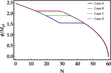
(a)

(b)

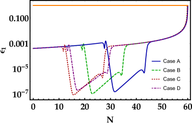
(c)

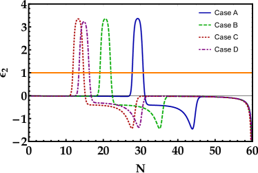
(d)

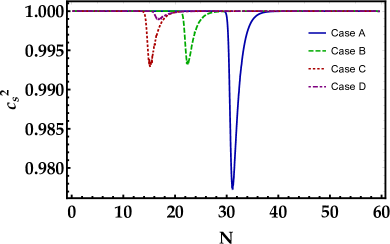
(e)

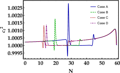
(f)

Figure 1: Evolutions of (a) the scalar filed $\phi$, (b) the Hubble parameter, (c) the first slow-roll parameter $\epsilon_{1}$, (d) the second slow-roll parameter $\epsilon_{2}$, (e) $c_{s}^{2}$, (f) $c_{t}^{2}$ versus the $e$-fold number $N$ for parameter sets in Table 1. The blue, green, red and purple lines are corresponding to $\rm{Case~{}}A$, $\rm{Case~{}}B$, $\rm{Case~{}}C$ and $\rm{Case~{}}D$, respectively.

III.1 Swampland’s criteria

Initially, we will introduce the swampland criteria and highlight the importance of incorporating these criteria in the analysis of inflationary models. The swampland criteria emerge from string theory and encompass two principal theoretical conjectures, known as distance and de Sitter conjectures as follows

$$\frac{|\Delta\phi|}{M_{\rm Pl}}\lesssim c_{1},\qquad\qquad M_{\rm Pl}\left|\frac{V_{,\phi}}{V}\right|\gtrsim c_{2},$$ (29)

where $c_{1}$ and $c_{2}$ are constant parameters. We investigate the validity of these conjectures for our model. Recent findings suggest that the parameter $c_{1}\sim{\cal O}(1)$, and that $c_{2}$ can be positive and less than unity, with values around $c_{2}\sim{\cal O}(0.1-1)$. Figure 2 demonstrates the fulfillment of the de Sitter conjecture, where $M_{\rm Pl}|V_{,\phi}/V|$ is of the order of ${\cal O}(0.1)$. The discrepancy between de Sitter conjecture of the swampland criteria and the standard inflationary model is evident. The slow-roll condition in the standard inflationary model, denoted by $\epsilon_{V}\ll 1$, starkly contradicts the de-Sitter conjecture. In the standard inflationary model, the ratio of tensor to scalar perturbations is estimated as $r=16\epsilon_{V}$. Consequently, considering the definition of $\epsilon_{V}$ and the de-Sitter conjecture results in $r\gtrsim 8c_{2}^{2}$. Hence, taking the parameter $c_{2}\sim{\cal O}(0.1)$ yields $r\sim 0.08$, which is inconsistent with Planck measurements at the CMB scale. Our estimations indicate that in the present model, $\Delta\phi/M_{\rm Pl}\sim{\cal O}(1)$, confirming the distance conjecture of the swampland criteria akrami:2020 ; Agazie1:2023 ; Agazie2:2023 ; Agazie3:2023 ; Agazie4:2023 . Therefore, it is clear from Fig. 2 that the model exhibits acceptable agreement with the swampland criteria.

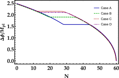
(a)

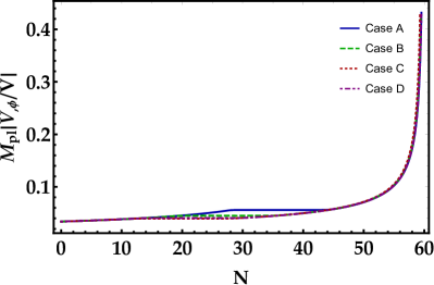
(b)

Figure 2: Validity of the swampland criteria for our model. (a) $\Delta\phi=\phi(N)-\phi(N_{\rm end})$, and (b) $M_{\rm Pl}|V_{,\phi}/V|$ versus the $e$-fold number $N$. The blue, green, red and purple lines are corresponding to $\rm{Case~{}}A$, $\rm{Case~{}}B$, $\rm{Case~{}}C$ and $\rm{Case~{}}D$, respectively.

III.2 Results for ${\cal P}_{s}$ and ${\cal P}_{t}$

As mentioned, after solving the MS Eq. (6), the value of the scalar power spectrum is determined. Furthermore, in Fig. 3, we depict the evolution of ${\cal P}_{s}$ for all parameter sets listed in Table 1. The curves in Fig. 3 are generated based on the mathematical calculations mentioned earlier and utilizing Eq. (11). The results demonstrate that the scalar power spectrum aligns with CMB measurements at the pivot scale. Additionally, ${\cal P}_{s}$ exhibits a significant enhancement by approximately seven orders of magnitude at small scales for PBHs formation.

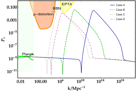
Figure 3: The scalar power spectra ${\cal P}_{s}$ in terms of wavenumber $k$ for the parameter sets listed in Table 1. The blue, green, red and purple lines are corresponding to $\rm{Case~{}}A$, $\rm{Case~{}}B$, $\rm{Case~{}}C$ and $\rm{Case~{}}D$, respectively. The CMB observations exclude the light-green shaded region akrami:2020 . The orange region shows the $\mu$-distortion of CMB Fixsen:1996 . The cyan area represents the effect on the ratio between neutron and proton during the big bang nucleosynthesis (BBN) Inomata:2016 . The EPTA observations constrain the yellow area Inomata:2019-a .

Similarly, by solving Eq. (19) the precise value of the tensor power spectrum ${\cal P}_{t}$ is obtained for the parameter sets listed in Table 1. The results for all parameter sets are depicted in Fig. 4. It should be noted that the value of the tensor to scalar ratio $r$, which is obtained from the exact solutions of Eqs. (11) and (21), on the CMB scale is consistent with the value obtained from the slow-roll approximation Eq. (24). It should be noted that the flat regions observed in ${\cal P}_{t}$ plots are due to the constancy of the Hubble parameter during the USR phase (see Fig. 1(b)). Furthermore, the minor fluctuations observed in ${\cal P}_{t}$ stem from the oscillatory behavior of $c_{t}$ (see Fig. 1(f)).

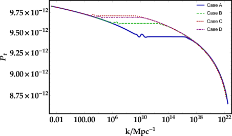
Figure 4: The tensor power spectra ${\cal P}_{t}$ in terms of wavenumber $k$ for the parameter sets listed in Table 1. The blue, green, red and purple lines are corresponding to $\rm{Case~{}}A$, $\rm{Case~{}}B$, $\rm{Case~{}}C$ and $\rm{Case~{}}D$, respectively.

IV The Abundance of PBHs

The objective of this section is to estimate the abundance of PBHs. It is established that overdense regions can form during the RD era as a result of the reentry of enhanced curvature perturbations into the horizon. Subsequently, these overdense regions may undergo gravitational collapse, leading to the formation of PBHs. The mass of PBHs is contingent upon the horizon mass and determined by

$$M(k)\simeq M_{\odot}\left(\frac{\gamma}{0.2}\right)\left(\frac{10.75}{g_{*}}\right)^{1/6}\left(\frac{k}{1.9\times 10^{6}\rm Mpc^{-1}}\right)^{-2},$$ (30)

where, $\gamma=(\frac{1}{\sqrt{3}})^{3}$ carr:1975 denotes the collapse efficiency, $g_{*}=106.75$ signifies the effective number of relativistic species at thermalization during the RD era. The formation rate for PBHs with mass $M(k)$ is determined utilizing the Press-Schechter theory, under the assumption of Gaussian statistics for the distribution of curvature perturbations as follows Tada:2019 ; young:2014

$$\beta(M)=\int^{\infty}_{\delta_{c}}\frac{{\rm d}\delta}{\sqrt{2\pi\sigma^{2}(M)}}\exp\left(\frac{-\delta^{2}}{2\sigma^{2}(M)}\right).$$ (31)

Here, $\delta_{c}$ denotes the threshold value of density perturbations required for PBHs production. In this analysis, we adopt $\delta_{c}=0.4$ based on previous studies Musco:2013 ; Harada:2013 . Additionally, the coarse-grained density contrast $\sigma^{2}(M)$, with the smoothing scale $k$, is defined as follows

$$\sigma_{k}^{2}=\left(\frac{2}{3}\right)^{4}\int^{\infty}_{0}\frac{{\rm d}q}{q}W^{2}(q/k)(q/k)^{4}{\cal P}_{s}(q),$$ (32)

where ${\cal P}_{s}$ indicates the curvature power spectrum, and $W$ is the Gaussian window function, which is given by $W(x)=\exp{\left(-x^{2}/2\right)}$. The ratio of the density parameters of PBHs $(\Omega_{\rm{PBH}})$ to that of dark matter $(\Omega_{\rm{DM}})$ in the universe at the present time, is given by the following PBHs abundance factor

$$f_{\rm{PBH}}(M)\simeq\frac{\Omega_{\rm{PBH}}}{\Omega_{\rm{DM}}}=\frac{\beta(M)}{1.84\times 10^{-8}}\left(\frac{\gamma}{0.2}\right)^{3/2}\left(\frac{g_{*}}{10.75}\right)^{-1/4}\left(\frac{0.12}{\Omega_{\rm{DM}}h^{2}}\right)\left(\frac{M}{M_{\odot}}\right)^{-1/2},$$ (33)

where $M$ is given by Eq. (30). The current density parameter of dark matter is determined as $\Omega_{\rm DM_{0}}h^{2}=0.12$ based on Planck 2018 data akrami:2020 . Utilizing ${\cal P}_{s}$ from solving the MS Eq. (6) and using Eqs. (30)-(33), we can calculate the abundance of PBHs for four cases listed in Tables 1. The numerical results are reported in Table 2 as well as Fig. 5.

As illustrated in Fig. 5, Case A corresponding to PBHs within the mass range of $10^{-13}M_{\odot}$, constitutes approximately $99\%$ of the total dark matter content of the universe. In Case B, the abundance of PBHs is $f_{\text{PBH}}^{\text{peak}}=0.0546$ within the mass range of $10^{-6}M_{\odot}$. Additionally, the abundances of this case fall within the permissible region of the observed microlensing events in the OGLE data. Moreover, PBHs in Case C are generated with mass about $14.38M_{\odot}$, features $f_{\text{PBH}}^{\text{peak}}=0.0023$. As depicted in Fig. 5, this category of PBHs is constrained by the upper limit of LIGO-Virgo observations. Finally, for Case D, the fractional abundance of PBHs is determined to be approximately $f_{\text{PBH}}^{\text{peak}}\simeq 0$, indicating that its contribution to dark matter is negligible. However, the spectrum of the produced GWs from this case is consistent with the NANOGrav 15 years data.

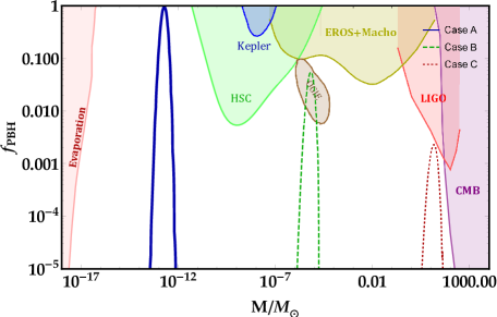
Figure 5: The abundances of PBHs with respect to their masses $M$ for the parameter sets listed in Table 1. The blue, green and red lines in the figure are corresponding to $\rm{Case~{}}A$, $\rm{Case~{}}B$ and $\rm{Case~{}}C$, respectively. The shaded regions represent recent observational constraints on the fractional abundance of PBHs. The purple area depicts the restriction on CMB from the signature of spherical accretion of PBHs inside halos CMB . The upper bound on the abundance of PBHs is shown by the border of the red shaded region and is derived from the LIGO-VIRGO event consolidation rate Abbott:2019 ; Chen:2022 ; Boehm:2021 ; Kavanagh:2018 . The brown shaded region represents the authorized region for PBHs abundance due to ultrashort-timescale microlensing events in the OGLE data OGLE . The green shaded area corresponds to constraints on microlensing events from collaborations between MACHO Alcock:2001 , EROS EORS , Kepler Kepler ), Icarus Icarus , and Subaru-HSC subaro . The pink shaded region delineates constraints related to PBHs evaporation such as extragalactic $\gamma$-ray background EGG , galactic center $511$ $keV$ $\gamma$-ray line (INTEGRAL) (Laha:2019, ), and effects on CMB spectrum Clark .

V Investigation of Secondary GWs

Gravitational waves are produced when enhanced primordial curvature perturbations re-enter the horizon during the RD era. These GWs can be detected by detectors with varying sensitivity ranges Inomata:2019-a ; Matarrese:1998 ; Mollerach:2004 ; Saito:2009 ; Garcia:2017 ; Cai:2019-a ; Cai:2019-b ; Cai:2019-c ; Bartolo:2019-a ; Bartolo:2019-b ; Wang:2019 ; Fumagalli:2020b ; Domenech:2020a ; Domenech:2020b ; Hajkarim:2019 ; Kohri:2018 ; Xu:2020 ; Fu:2020 . In this discussion, we examine the generation of secondary GWs within the GB framework, incorporating low-scale SB SUSY potential. Upon the end of the inflationary phase, the inflaton field decays and converts into light particles, which heat the universe and initiate the RD epoch. Consequently, the inflaton field has a negligible impact on cosmic evolution during the RD epoch. Therefore, the standard Einstein formulation can be employed to investigate the production of secondary GWs during this era. Therefore, during the RD era, the energy density parameter of GWs can be calculated as follows Ananda:2007 ; Baumann:2007 ; Kohri:2018 ; Lu:2019

$$\Omega_{\rm GW}(k,\eta)=\frac{1}{6}\left(\frac{k}{aH}\right)^{2}\int_{0}^{\infty}dv\int_{|1-v|}^{|1+v|}du\left(\frac{4v^{2}-\left(1-u^{2}+v^{2}\right)^{2}}{4uv}\right)^{2}\overline{I_{RD}^{2}(u,v,x)}\mathcal{P}_{s}(ku)\mathcal{P}_{s}(kv),$$ (34)

where $\eta$ represents the conformal time, and the time-averaged value of the source terms is expressed as follows

$$\overline{I_{\rm RD}^{2}(u,v,x\to\infty)}= \frac{1}{2x^{2}}\Bigg{[}\left(\frac{3\pi\left(u^{2}+v^{2}-3\right)^{2}\Theta\left(u+v-\sqrt{3}\right)}{4u^{3}v^{3}}+\frac{T_{c}(u,v,1)}{9}\right)^{2} +\left(\frac{\tilde{T}_{s}(u,v,1)}{9}\right)^{2}\Bigg{]}.$$ (35)

Here, $\Theta$ denotes the Heaviside theta function which is defined as $\Theta(x\geq 0)=1$ and $\Theta(x<0)=0$. Additionally, the functions utilized within Eq. (35) are defined as follows

$$T_{c}= -\frac{27}{8u^{3}v^{3}x^{4}}\Bigg{\{}-48uvx^{2}\cos\left(\frac{ux}{\sqrt{3}}\right)\cos\left(\frac{vx}{\sqrt{3}}\right)\left(3\sin(x)+x\cos(x)\right)+$$

$$48\sqrt{3}x^{2}\cos(x)\left(v\sin\left(\frac{ux}{\sqrt{3}}\right)\cos\left(\frac{vx}{\sqrt{3}}\right)+u\cos\left(\frac{ux}{\sqrt{3}}\right)\sin\left(\frac{vx}{\sqrt{3}}\right)\right)+$$

$$8\sqrt{3}x\sin(x)\Bigg{[}v\left(18-x^{2}\left(u^{2}-v^{2}+3\right)\right)\sin\left(\frac{ux}{\sqrt{3}}\right)\cos\left(\frac{vx}{\sqrt{3}}\right)+$$

$$u\left(18-x^{2}\left(-u^{2}+v^{2}+3\right)\right)\cos\left(\frac{ux}{\sqrt{3}}\right)\sin\left(\frac{vx}{\sqrt{3}}\right)\Bigg{]}+$$

$$24x\cos(x)\left(x^{2}\left(-u^{2}-v^{2}+3\right)-6\right)\sin\left(\frac{ux}{\sqrt{3}}\right)\sin\left(\frac{vx}{\sqrt{3}}\right)+$$

$$24\sin(x)\left(x^{2}\left(u^{2}+v^{2}+3\right)-18\right)\sin\left(\frac{ux}{\sqrt{3}}\right)\sin\left(\frac{vx}{\sqrt{3}}\right)\Bigg{\}}$$

$$-\frac{\left(27\left(u^{2}+v^{2}-3\right)^{2}\right)}{4u^{3}v^{3}}\Bigg{\{}\text{Si}\left[\left(\frac{u-v}{\sqrt{3}}+1\right)x\right]-\text{Si}\left[\left(\frac{u+v}{\sqrt{3}}+1\right)x\right]$$

$$+\text{Si}\left[\left(1-\frac{u-v}{\sqrt{3}}\right)x\right]-\text{Si}\left[\left(1-\frac{u+v}{\sqrt{3}}\right)x\right]\Bigg{\}},$$ (36)

$$T_{s}= \frac{27}{8u^{3}v^{3}x^{4}}\Bigg{\{}48uvx^{2}\cos\left(\frac{ux}{\sqrt{3}}\right)\cos\left(\frac{vx}{\sqrt{3}}\right)\left(x\sin(x)-3\cos(x)\right)-$$

$$48\sqrt{3}x^{2}\sin(x)\left(v\sin\left(\frac{ux}{\sqrt{3}}\right)\cos\left(\frac{vx}{\sqrt{3}}\right)+u\cos\left(\frac{ux}{\sqrt{3}}\right)\sin\left(\frac{vx}{\sqrt{3}}\right)\right)+$$

$$8\sqrt{3}x\cos(x)\Bigg{[}v\left(18-x^{2}\left(u^{2}-v^{2}+3\right)\right)\sin\left(\frac{ux}{\sqrt{3}}\right)\cos\left(\frac{vx}{\sqrt{3}}\right)+$$

$$u\left(18-x^{2}\left(-u^{2}+v^{2}+3\right)\right)\cos\left(\frac{ux}{\sqrt{3}}\right)\sin\left(\frac{vx}{\sqrt{3}}\right)\Bigg{]}+$$

$$24x\sin(x)\left(6-x^{2}\left(-u^{2}-v^{2}+3\right)\right)\sin\left(\frac{ux}{\sqrt{3}}\right)\sin\left(\frac{vx}{\sqrt{3}}\right)+$$

$$24\cos(x)\left(x^{2}\left(u^{2}+v^{2}+3\right)-18\right)\sin\left(\frac{ux}{\sqrt{3}}\right)\sin\left(\frac{vx}{\sqrt{3}}\right)\Bigg{\}}-\frac{27\left(u^{2}+v^{2}-3\right)}{u^{2}v^{2}}+$$

$$\frac{\left(27\left(u^{2}+v^{2}-3\right)^{2}\right)}{4u^{3}v^{3}}\Bigg{\{}-\text{Ci}\left[\left|1-\frac{u+v}{\sqrt{3}}\right|x\right]+\ln\left|\frac{3-(u+v)^{2}}{3-(u-v)^{2}}\right|+$$

$$\text{Ci}\left[\left(\frac{u-v}{\sqrt{3}}+1\right)x\right]-\text{Ci}\left[\left(\frac{u+v}{\sqrt{3}}+1\right)x\right]+\text{Ci}\left[\left(1-\frac{u-v}{\sqrt{3}}\right)x\right]\Bigg{\}}.$$ (37)

Moreover, the sine-integral $\text{Si}(x)$ and cosine-integral $\text{Ci}(x)$ functions are defined as

$$\text{Si}(x)\equiv\int_{0}^{x}\frac{\sin(y)}{y}dy,\qquad\text{Ci}(x)\equiv-\int_{x}^{\infty}\frac{\cos(y)}{y}dy.$$ (38)

The function $\tilde{T}_{s}(u,v,1)$ from Eq. (35), is expressed as

$$\tilde{T}_{s}(u,v,1)=T_{s}(u,v,1)+\frac{27\left(u^{2}+v^{2}-3\right)}{u^{2}v^{2}}-\frac{27\left(u^{2}+v^{2}-3\right)^{2}}{4u^{3}v^{3}}\ln\left|\frac{3-(u+v)^{2}}{3-(u-v)^{2}}\right|.$$ (39)

The current energy spectrum of the GWs is defined as follows Inomata:2019-a

$$\Omega_{\rm GW_{0}}h^{2}=0.83\left(\frac{g_{*}}{10.75}\right)^{-1/3}\Omega_{\rm r_{0}}h^{2}\Omega_{\rm{GW}}(\eta_{c},k)\,,$$ (40)

wherein, $\Omega_{\rm{r_{0}}}h^{2}\simeq 4.2\times 10^{-5}$ represents the radiation density parameter at the current epoch, and $g_{*}\simeq 106.75$ denotes the effective degrees of freedom in the energy density at $\eta_{c}$. Also, the frequency in terms of the wavenumber reads

$$f=1.546\times 10^{-15}\left(\frac{k}{{\rm Mpc}^{-1}}\right){\rm Hz}.$$ (41)

Finally, we can evaluate the current energy density parameter of generated GWs from PBHs formation in our model by utilizing the power spectrum derived from the MS Eq. (6) and using Eqs. (34)-(41). Our results, accompanied by the sensitivity curves of various GWs observatories, are illustrated in Fig. 6. For Cases A, B, C, and D, the spectra of $\Omega_{\rm GW_{0}}$ are located at different frequencies. About Case A, associated with asteroid-mass PBHs, the peak of $\Omega_{\rm GW_{0}}$ spectrum is observed in the mHz frequency ranges, detectable by observatories such as LISA ligo-a ; ligo-b ; lisa ; lisa-a , BBO Yagi:2011BBODECIGO ; Yagi:2017BBODECIGO ; Harry:2006BBO ; Crowder:2005BBO ; Corbin:2006BBO , and DECIGO Yagi:2017BBODECIGO ; Seto:2001DECIGO ; Kawamura:2006DECIGO ; Kawamura:2011DECIGO . For Cases B and C, corresponding to earth-mass and stellar-mass PBHs, the peaks of $\Omega_{\rm GW_{0}}$ are, respectively, centered around $f_{c}\sim 10^{-6}\text{Hz}$ and $f_{c}\sim 10^{-10}\text{Hz}$, falling within the sensitivity range of the SKA observatory ska ; skaCarilli:2004 ; skaWeltman:2020 . Note that the spectrum of $\Omega_{\rm GW_{0}}$ for Case D intersect the sensitive regions of the PPTA and NANOGrav detectors (See Fig. 6).

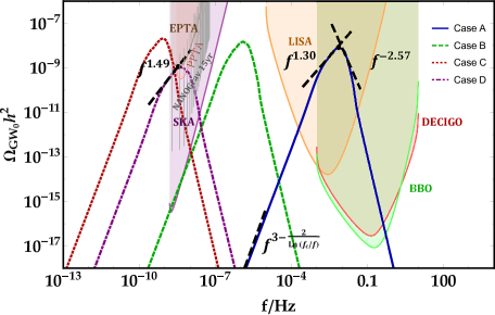
Figure 6: The spectra of the present energy density parameter of the secondary gravitational waves $\Omega_{\rm GW_{0}}$ with regard to frequency pertinent to the low-scale SB SUSY potential in the GB framework for parameter sets of Table 1. The blue, green, red and purple lines are corresponding to $\rm{Case~{}}A$, $\rm{Case~{}}B$, $\rm{Case~{}}C$ and $\rm{Case~{}}D$, respectively. The accuracy of our predictions can be verified by observatories such as the European PTA (EPTA) EPTA-a ; EPTA-b ; EPTA-c ; EPTA-d , the Square Kilometer Array (SKA) ska ; skaCarilli:2004 ; skaWeltman:2020 , Laser Interferometer Space Antenna (LISA) ligo-a ; ligo-b ; lisa ; lisa-a , BBO observatories Yagi:2011BBODECIGO ; Yagi:2017BBODECIGO ; Harry:2006BBO ; Crowder:2005BBO ; Corbin:2006BBO , DECIGO Yagi:2011BBODECIGO ; Yagi:2017BBODECIGO ; Seto:2001DECIGO ; Kawamura:2006DECIGO ; Kawamura:2011DECIGO , and the NANOGrav 15 years data Agazie1:2023 ; Agazie2:2023 ; Agazie3:2023 ; Agazie4:2023 .

The predicted $\Omega_{\rm GW_{0}}$ spectra for all cases in our model intersect the sensitivity curves of various gravitational wave observatories. Consequently, the validity of this model can be assessed using data from these observatories, both in the present and the future. Lastly, we scrutinize the behavior of the $\Omega_{\rm GW_{0}}$ spectra across different frequency ranges. It has been verified that in proximity to the peak position, the current density parameter spectrum of secondary GWs demonstrates a power-law behavior concerning frequency, i.e., $\Omega_{\rm GW_{0}}(f)\sim f^{n}$ Fu:2019vqc ; Fu:2020lob ; Bagui:2021dqi ; Xu ; Kuroyanagi . The precise values of the critical frequencies and peak heights for all cases are reported in Table 3. Furthermore, our results in the infrared regime $f\ll f_{c}$ obey the analytical relation $\Omega_{\rm GW_{0}}\sim f^{3-2/\ln\left(f_{c}/f\right)}$ derived by Yuan:2020 ; Sasaki:2020 , as depicted in Fig. 6.

Table 3: The frequencies and heights of the peaks of the $\Omega_{\rm GW_{0}}$ spectra beside power index $n$ in frequency ranges $f\ll f_{c}$, $f<f_{c}$ and $f>f_{c}$ for all Cases.

#	$f_{c}$	$\Omega_{\rm GW_{0}}\left(f_{c}\right)$	$n_{f\ll f_{c}}$	$n_{f<f_{c}}$	$n_{f>f_{c}}$
$\rm{Case~{}}A$	$7.353\times 10^{-3}$	$8.441\times 10^{-9}$	$3.0$	$1.30$	$-2.57$
$\rm{Case~{}}B$	$1.231\times 10^{-6}$	$1.507\times 10^{-8}$	$2.92$	$1.33$	$-1.87$
$\rm{Case~{}}C$	$8.354\times 10^{-10}$	$2.064\times 10^{-8}$	$2.82$	$1.09$	$-1.70$
$\rm{Case~{}}D$	$3.379\times 10^{-9}$	$1.157\times 10^{-9}$	$2.84$	$1.49$	$-1.27$

In our model, the detection of induced GW signals presents a unique opportunity to discern the presence of PBHs. Recently, the NANOGrav pulsar timing array team unveiled low-frequency stochastic gravitational wave background through 15 years of data collection Agazie1:2023 ; Agazie2:2023 ; Agazie3:2023 ; Agazie4:2023 . As mentioned, the spectra of $\Omega_{\rm GW_{0}}$ for Case D intersect the sensitivity ranges of the PPTA and NANOGrav detectors (refer to Fig. 6). The PTA GWs signal around the nano-Hz regime can be parameterized as $\Omega_{\rm{GW}}(f)\sim f^{5-\gamma}$, where $\gamma$ is the spectral index. The NANOGrav collaboration reports the best-fit value for the spectral index as $\gamma=3.2\pm 0.6$ BabichevFitNANOGrav:2023 ; VagnozziFitNANOGrav:2023 ; AntoniadisFitNANOGrav:2023a ; AntoniadisFitNANOGrav:2023b ; AntoniadisFitNANOGrav:2023c . For Case D, our numerical result for $\gamma=5-n=3.51$, is consistent with the observed findings.

VI Results and discussion

This study explored PBHs formation within an inflationary framework involving a coupling between the scalar field and the GB term. Moreover, we examined the low-scale SB SUSY potential within this context. In the presence of the GB coupling term, the inflaton traverses near a non-trivial fixed point and undergoes an USR epoch. Consequently, the primordial curvature perturbations can experience enhancement during this era. The low-scale SB SUSY potential in the standard framework of inflation is ruled out by the Planck 2018 observations akrami:2020 . This characteristic led us to reconsider it within the GB framework to attain a viable inflationary model. By employing the GB coupling term and adjusting the model parameters ($M$, $\beta$, $\xi_{0}$, $\xi_{1}$, $\phi_{c}$, $V_{0}$, $\alpha$), we effectively aligned the SB SUSY potential with the findings of CMB measurements. In addition, during the USR phase, the amplitude of perturbations can increase, leading to the production of PBHs. Utilizing the precise solution of the background equations, we illustrated the evolution of the inflaton field $\phi$, the Hubble parameter $H$, the slow-roll parameters $(\epsilon_{1}$ and $\epsilon_{2}$), $c_{s}^{2}$, and $c_{t}^{2}$ in Fig. 1 as functions of the number of $e$-folds. It is evident from this figure that during the USR phase, the slow-roll conditions are upheld by the first parameter ($\epsilon_{1}\ll 1$) and violated by the second parameter ($\left|\epsilon_{2}\right|\geq 1$). In this regard, we derived the numerical solution of the MS Eq. (6) to compute the precise values of the scalar power spectra ${\cal P}_{s}$ for all cases listed in Table 1. Furthermore, Figure 3 illustrates that the obtained power spectra are consistent with Planck 2018 data on large scales and exhibit peaks of adequate amplitude to facilitate the generation of PBHs on small scales. Our calculations yield $n_{s}=0.970$, that aligns with $68\,\%\,\rm CL$ of the Planck 2018 TT, TE, EE + lowE + lensing + BK18 + BAO akrami:2020 ; Campeti:2022 , and $r=0.005$, which aligns with the BICEP/Keck 2018 data ($r<0.036$ at $95\,\%\,\rm CL$) akrami:2020 ; Ade:2021 . Hence, through the utilization of the GB framework the SB SUSY potential is revitalized. Moreover, this choice enables us to generate PBHs with suitable abundance and GWs within the sensitivity range of observatories. Also, our analysis confirms that our model satisfies the swampland criteria. In Fig. 5, Case A corresponding to PBHs with masses around $10^{-13}M_{\odot}$, constituting nearly all of the dark matter. In Case B, PBH abundance peaks at $f_{\text{PBH}}^{\text{peak}}=0.0546$ for masses around $10^{-6}M_{\odot}$, aligning with observed microlensing events in OGLE data. Case C features PBHs with a mass of approximately $14.38M_{\odot}$ and a peak abundance $f_{\text{PBH}}^{\text{peak}}=0.0023$, constrained by upper limits from LIGO-Virgo observations. In Case D, the fractional abundance of PBHs is approximately $f_{\text{PBH}}^{\text{peak}}\simeq 0$, indicating a negligible contribution of dark matter. However, the produced spectrum of GWs from this case aligns with NANOGrav 15 years data. Lastly, we examined the production of induced GWs subsequent to the formation of PBHs for all cases of our model. In Case A, linked to asteroid-mass PBHs, the peak of $\Omega_{\rm GW_{0}}$ spectrum occurs in the mHz frequency range, detectable by LISA, BBO, and DECIGO. For Cases B and C, linked to Earth-mass and stellar-mass PBHs respectively, the spectral peaks are near $f_{c}\sim 10^{-6}$ Hz and $f_{c}\sim 10^{-10}$ Hz, within the sensitivity range of the SKA observatory. Additionally, the spectrum of $\Omega_{\rm GW_{0}}$ for Case D intersects the sensitivity ranges of the PPTA and NANOGrav detectors (refer to Fig. 6). Therefore, evaluating the credibility of our model can be accomplished by analyzing GWs using the data extracted from these detectors. In the final phase, we calculated the power-law behaviour of $\Omega_{\rm GW_{0}}$ spectra ($\Omega_{\rm GW_{0}}(f)\sim f^{n}$) for all Cases across different frequency ranges. Table 3 presents the peak frequencies of $\Omega_{\rm GW_{0}}$ spectra and the estimated values for the power indices, $n$, for all cases in three frequency regions $f\ll f_{c}$, $f<f_{c}$, and $f>f_{c}$. It can be deduced that the resulting values for $n$ in the infrared region $f\ll f_{c}$ could align with the logarithmic equation $n=3-2/\ln(f_{c}/f)$. In Case D, our numerical estimation for $\gamma=5-n=3.51$ aligns with the observed results from NANOGrav 15-year data.

References

- (1) Ya. B. Zel’dovich, and I. D. Novikov, Sov. Astron. 10, 602 (1967).
- (2) S. Hawking, Mon. Not. R. Astron. Soc. 152, 75 (1971).
- (3) S. Hawking, Nature 248, 30 (1974).
- (4) S. Hawking, Commun. Math. Phys. 46, 206 (1976).
- (5) B. J. Carr, Astrophys. J. 201, 1 (1975).
- (6) B. J. Carr, and S.W. Hawking, Mon. Not. R. Astron. Soc. 168, 399 (1974).
- (7) D. N. Page, and S. Hawking, Astrophys. J. 206, 1 (1976).
- (8) G. J. Olmo, Int. J. Mod. Phys. D 20 (2011).
- (9) A. de la Cruz-Dombriz, and D. Saez-Gomez, Entropy 14, 1717 (2012).
- (10) G. F. Chapline, Nature 253, 251 (1975).
- (11) A. G. Polnarev, and M. Y. Khlopov, Sov. Phys. Usp. 28, 213 (1985).
- (12) P. Ivanov, P. Nasselsky, and I. D. Novikov, Phys. Rev. D 50, 7173 (1994).
- (13) S. Capozziello, and M. De Laurentis, Phys. Rep. 509 (2011).
- (14) S. Nojiri, and S. D. Odintsov, Phys. Rep. 505 (2011).
- (15) S. Nojiri, S. D. Odintsov, and V. K. Oikonomou, Phys. Rept. 692 (2017).
- (16) S. Choudhury, and A. Mazumdar, Phys. Lett. B 733, 270 (2014).
- (17) M. Solbi, and K. Karami, Eur. Phys. J. C 81, 884 (2021).
- (18) M. Solbi, and K. Karami, J. Cosmol. Astropart. Phys. 08, 056 (2021).
- (19) Z. Teimoori, K. Rezazadeh, M. A. Rasheed, and K. Karami, J. Cosmol. Astropart. Phys. 10, 018 (2021).
- (20) K. Rezazadeh, Z. Teimoori, and K. Karami, Eur. Phys. J. C 82, 758 (2022).
- (21) Y. Cai, and Y. S. Piao, Phys. Rev. D 103, 083521 (2021).
- (22) A. Chakraborty, P. K. Chanda, K. L. Pandey, and S. Das, Astrophys. J. 932, 119 (2022).
- (23) T. Papanikolaou, C. Tzerefos, S. Basilakos, and E. N. Saridakis, J. Cosmol. Astropart. Phys. 2022, 13 (2022).
- (24) T. Papanikolaou, C. Tzerefos, S. Basilakos, and E. N. Saridakis, Eur. Phys. J. C 83, 31 (2023).
- (25) T. Papanikolaou, A. Lymperis, S. Lolab, and E. N. Saridakis, J. Cosmol. Astropart. Phys. 03, 003 (2023).
- (26) G. Domènech, G. Vargas, and T. Vargas, J. Cosmol. Astropart. Phys. 03, 002 (2024).
- (27) Y. Cai, M. Zhu, and Y. S. Piao, arXiv:2305.10933.
- (28) B. P. Abbott et al., (LIGO Scientific and Virgo Collaborations) Phys. Rev. D 93, 122004 (2016).
- (29) B. P. Abbott et al., (LIGO Scientific Collaboration and Virgo Collaboration), Phys. Rev. Lett. 116, 061102 (2016).
- (30) B. P. Abbott et al., (LIGO Scientific Collaboration and Virgo Collaboration), Phys. Rev. Lett. 116, 241103 (2016).
- (31) B. P. Abbott et al., Astrophys. J. Lett. 848, L12 (2017).
- (32) B. P. Abbott et al., (LIGO Scientific Collaboration and Virgo Collaboration), Phys. Rev. Lett. 116, 221101 (2017).
- (33) B. P. Abbott et al., (LIGO Scientific Collaboration and Virgo Collaboration), Astrophys. J. 851, L35 (2017).
- (34) B. P. Abbott et al., (LIGO Scientific Collaboration and Virgo Collaboration), Phys. Rev. Lett. 119, 141101 (2017).
- (35) B. P. Abbott, et al., (LIGO Scientific Collaboration and Virgo Collaboration), Phys. Rev. Lett. 123, 161102 (2019).
- (36) H. Niikura et al., Phys. Rev. D 99, 083503 (2019).
- (37) C. Alcock et al., Astrophys. J. Lett. 550, L169 (2001).
- (38) A. Gould, Astrophys. J. 386, L5 (1992).
- (39) S. Heydari, and K. Karami, Eur. Phys. J. C 82, 83 (2022).
- (40) S. Heydari, and K. Karami, Eur. Phys. J. C 84, 127 (2024).
- (41) S. Heydari, and K. Karami, J. Cosmol. Astropart. Phys. 02, 047 (2024).
- (42) J. J. Dalcanton et al., Astrophys. J. 424, 550 (1994).
- (43) G. Sato-Polito, E. D. Kovetz, and M. Kamionkowski, Phys. Rev. D 100, 063521 (2019).
- (44) D. M. Jacobs et al., Mon. Not. Roy. Astron. Soc. 450, 3418 (2015).
- (45) Y. Ali-Haimoud, and M. Kamionkowski, Phys. Rev. D 95, 043534 (2017).
- (46) S. Wang, Y. F. Wang, Q. G. Huang, and T. G. F. Li, Phys. Rev. Lett. 120, 191102 (2018).
- (47) R. Laha, J. B. Munoz, and T. R. Slatyer, Phys. Rev. D 101, 123514 (2020).
- (48) Z. Teimoori, K. Rezazadeh, and K. Karami, Astrophys. J. 915, 118 (2021).
- (49) S. Heydari, and K. Karami, arXiv:2405.08563.
- (50) S. Heydari, and K. Karami, J. Cosmol. Astropart. Phys. 03, 033 (2022).
- (51) M. Solbi, and K. Karami, arXiv:2403.00021.
- (52) Y. Akrami et al., (Planck Collaboration), Astron. Astrophys. 641, A10 (2020).
- (53) I. Dalianis, A. Kehagias, and G. Tringas, J. Cosmol. Astropart. Phys. 01, 037 (2019).
- (54) R. Mahbub, Phys. Rev. D 101, 023533 (2020).
- (55) A. Y. Kamenshchik, A. Tronconi, T. Vardanyan, and G. Venturi, Phys. Lett. B 791, 201 (2019).
- (56) S. Kawai, and J. Kim, Phys. Rev. D 104, 083545 (2021).
- (57) F. Zhang, Phys. Rev. D 105, 063539 (2022).
- (58) R. Kawaguchi, and Sh. Tsujikawa, Phys. Rev. D 107, 063508 (2023).
- (59) A. Ashrafzadeh, and K. Karami, Astrophys. J. 965, 11 (2024).
- (60) C. Fu, P. Wu, and H. Yu, Phys. Rev. D 100, 063532 (2019).
- (61) S. S. Mishra, and V. Sahni, J. Cosmol. Astropart. Phys. 04, 007 (2020).
- (62) P. Villanueva-Domingo, O. Mena, and S. Palomares-Ruiz, Front. Astron. Space. Sci. 8, 103389 (2021).
- (63) Q. Gao, Y. Gong, and Zh. Yi, Nucl. Phys. B 969, 115480 (2021).
- (64) J. Lin et al., Phys. Rev. D 101, 103515 (2020).
- (65) S. Choudhury, S. Panda, and M. Sami, Phys. Lett. B 845, 138123 (2023).
- (66) S. Bhattacharya et al., Galaxies 11, 35 (2023).
- (67) S. Mittal, A. Ray, G. Kulkarni and B. Dasgupta, J. Cosmol. Astropart. Phys. 2022, 30 (2022).
- (68) G. Domènech, Universe. 7, 398 (2021).
- (69) G. Domènech, Ch. Lin, and M. Sasaki, J. Cosmol. Astropart. Phys. 04, 062 (2021).
- (70) G. Domènech, and M. Sasaki, Class. Quantum Grav. 41, 143001 (2024).
- (71) M. R. Gangopadhyay et al., arXiv:2309.03101.
- (72) G. Bhattacharya et al., arXiv:2309.00973.
- (73) N. Bartolo et al., Phys. Rev. Lett. 122, 211301 (2019).
- (74) N. Bartolo et al., Phys. Rev. D 99, 103521 (2019).
- (75) R. G. Cai, S. Pi, and M. Sasaki, Phys. Rev. Lett. 122, 201101 (2019).
- (76) J. Fumagalli, S. Renaux-Petel, and L. T. Witkowski, J. Cosmol. Astropart. Phys. 08, 030 (2021).
- (77) R. G. Cai, S. Pi, S. J. Wang, and X. Y. Yang, J. Cosmol. Astropart. Phys. 05, 013 (2019).
- (78) Y. F. Cai et al., Phys. Rev. D 100, 043518 (2019).
- (79) S. Wang, T. Terada, and K. Kohri, Phys. Rev. D 99, 103531 (2019).
- (80) G. Agazie et al., (NANOGrav Collaboration), Astrophys. J. Lett. 951, L11 (2023).
- (81) G. Agazie et al., (NANOGrav Collaboration), Astrophys. J. Lett. 951, L9 (2023).
- (82) G. Agazie et al., (NANOGrav Collaboration), Astrophys. J. Lett. 951, L10 (2023).
- (83) G. Agazie et al., (NANOGrav Collaboration), Astrophys. J. Lett. 951, L8 (2023).
- (84) H. V. Ragavendra et al., Galaxies 11, 34 (2023).
- (85) C. Lanczos, Ann. Math. 39, 842 (1938).
- (86) D. Lovelock, and J. Math. Phys. 12, 498 (1971).
- (87) N. Rashidi, and K. Nozari, Astrophys. J. 890, 58 (2020).
- (88) S. Azizi, S. Eslamzadeh, J. T. Firouzjaee, and K. Nozari, Nucl. Phys. B 985, 115993 (2022).
- (89) S. S. Shahraeini, K. Nozari, and S. Saghafi, J. Hologr. Appl. Phys. 2, 55 (2022).
- (90) R. C. Myers, and J. Z. Simon, Phys. Rev. D 38, 2434 (1988).
- (91) D. G. Boulware, and S. Deser, Phys. Rev. Lett. 55, 2656 (1985).
- (92) C. Sahabandu, P. Suranyi, C. Vaz, and L. C. R. Wijewardhana, Phys. Rev. D 73, 044009 (2006).
- (93) Y. M. Cho, and I. P. Neupane, Phys. Rev. D 66, 024044 (2002).
- (94) S. G. Ghosh, S. D. Maharaj, Phys. Rev. D 89, 084027 (2014).
- (95) S. H. Mazharimousavi, and M. Halilsoy, Phys. Lett. B 681, 190 (2009).
- (96) S. Das, Phys. Rev. D 99, 083510 (2019).
- (97) S. K. Garg, and C. Krishnan, J. High Energy Phys. 11, 075 (2019).
- (98) H. Ooguri, E. Palti, G. Shiu, and C. Vafa, Phys. Lett. B 788, 180 (2019).
- (99) A. Kehagias, and A. Riotto, Fortschr. Phys. 66, 1800052 (2018).
- (100) E. O. Pozdeeva, M. R. Gangopadhyay, M. Sami et al., Phys. Rev. D 102, 043525 (2020).
- (101) H. A. Khan, Phys. Rev. D 105, 063526 (2022).
- (102) M. R. Gangopadhyay, and H. A. Khan, Phys. Dark Universe 40, 101177 (2023).
- (103) S. D. Odintsov, V. K. Oikonomou, and F. P. Fronimos, Ann. Phys. 420, 168250 (2020).
- (104) S. D. Odintsov, V. K. Oikonomou, and F. P. Fronimos, Phys. Rev. D 107, 084007 (2023).
- (105) S. Nojiri, S. D. Odintsov, and D. S. Gòmez, Phys. Dark Universe 41, 101238 (2023).
- (106) P. X. Jiang, J. W. Hu, and Z. K. Guo, Phys. Rev. D 88, 123508 (2013).
- (107) S. Koh, Phys. Rev. D 90, 063527 (2014).
- (108) Z. K. Guo, Phys. Rev. D 81, 123520 (2010).
- (109) S. D. Odintsov, V. K. Oikonomou, and F. P. Fronimos, Nucl. Phys. B 958, 115135 (2020).
- (110) T. J. Gao, Eur. Phys. J. C 80, 1013 (2020).
- (111) A. De. Felice, and S. Tsujikawa, J. Cosmol. Astropart. Phys. 04, 029 (2011).
- (112) S. D. Odintsov, and V. K. Oikonomou, Phys. Lett. B 805, 135437 (2020).
- (113) G. W. Horndeski, Int. J. Theor. Phys. 10, 363 (1974).
- (114) P. Campeti, and E. Komatsu, Astrophys. J. 941, 110 (2022).
- (115) P. A. R. Ade et al., (BICEP/Keck Collaboration), Phys. Rev. Lett. 127, 151301 (2021).
- (116) G. R. Dvali, Q, Shafi, and R. K. Schaefer, Phys. Rev. Lett., 73, 1886 (1994).
- (117) E. J. Copeland, A. R. Liddle, D. H. Lyth, E. D. Stewart, and D. Wands, Phys. Rev. D, 49, 6410 (1994).
- (118) A. D. Linde, Phys. Rev. D, 49, 748 (1994).
- (119) D. J. Fixsen et al., Astrophys. J. 473, 576 (1996).
- (120) K. Inomata, M. Kawasaki, and Y. Tada, Phys. Rev. D 94, 043527 (2016).
- (121) K. Inomata, and T. Nakama, Phys. Rev. D 99, 043511 (2019).
- (122) Y. Tada, and S. Yokoyama, Phys. Rev. D 100, 023537 (2019).
- (123) S. Young, C. T. Byrnes, and M. Sasaki, J. Cosmol. Astropart. Phys. 07, 045 (2014).
- (124) T. Harada, C. M. Yoo, and K. Kohri, Phys. Rev. D 88, 084051 (2013).
- (125) I. Musco, and J. C. Miller, Class. Quant. Grav. 30, 145009 (2013).
- (126) P. D. Serpico, V. Poulin, D. Inman, and K. Kohri, Phys. Rev. Res. 2, 023204 (2020).
- (127) B. J. Kavanagh, D. Gaggero, and G. Bertone, Phys. Rev. D 98, 023536 (2018).
- (128) Z. C. Chen, Y. M. Wu, and Q. G. Huang, Astrophys. J. 936, 20 (2022).
- (129) C. Boehm et al., J. Cosmol. Astropart. Phys. 03, 078 (2021).
- (130) P. Tisserand et al., Astron. Astrophys. 469, 387 (2007).
- (131) K. Griest, A. M. Cieplak, and M. J. Lehner, Astrophys. J. 786, 158 (2014).
- (132) M. Oguri et al., Phys. Rev. D 97, 023518 (2018).
- (133) D. Croon, D. McKeen, N. Raj, and Z. Wang, Phys. Rev. D 102, 083021 (2020).
- (134) B. J. Carr et al., Phys. Rev. D 81, 104019 (2010).
- (135) R. Laha, Phys. Rev. Lett. 123, 251101 (2019).
- (136) S. Clark et al., Phys. Rev. D 95, 083006 (2017).
- (137) S. Matarrese, S. Mollerach, and M. Bruni, Phys. Rev. D 58, 043504 (1998).
- (138) S. Mollerach, D. Harari, and S. Matarrese, Phys. Rev. D 69, 063002 (2004).
- (139) R. Saito, and J. Yokoyama, Phys. Rev. Lett. 102, 161101 (2009.)
- (140) J. Garcia-Bellido, M. Peloso, and C. Unal, J. Cosmol. Astropart. Phys. 09, 013 (2017).
- (141) K. Kohri, and T. Terada, Phys. Rev. D 97, 123532 (2018).
- (142) R. G. Cai, S. Pi, and M. Sasaki, Phys. Rev. Lett. 122, 201101 (2019).
- (143) R. G. Cai, S. Pi, S. J. Wang, and X. Y. Yang, J. Cosmol. Astropart. Phys. 05, 013 (2019).
- (144) Y. F. Cai et al., Phys. Rev. D 100, 043518 (2019).
- (145) N. Bartolo et al., Phys. Rev. Lett. 122, 211301 (2019).
- (146) N. Bartolo et al., Phys. Rev. D 99, 103521 (2019).
- (147) J. Fumagalli, S. Renaux-Petel, and L. T. Witkowski, J. Cosmol. Astropart. Phys. 08, 030 (2021).
- (148) F. Hajkarim, and J. Schaffner-Bielich, Phys. Rev. D 101, 043522 (2020).
- (149) W. T. Xu, J. Liu, T. J. Gao, and Z. K. Guo, Phys. Rev. D 101, 023505 (2020).
- (150) C. Fu, P. Wu, and H. Yu, Phys. Rev. D 101, 023529 (2020).
- (151) G. Domènech, and M. Sasaki, Int. J. Mod. Phys. D 29, 2050028 (2020).
- (152) G. Domènech, and M. Sasaki, Phys. Rev. D 103, 063531 (2021).
- (153) Y. Lu, Y. Gong, Z. Yi, and F. Zhang, J. Cosmol. Astropart. Phys. 12, 031 (2019).
- (154) K. N. Ananda, C. Clarkson, and D. Wands, Phys. Rev. D 75, 123518 (2007).
- (155) D. Baumann et al., Phys. Rev. D 76, 084019 (2007).
- (156) G. M. Harry (LIGO Scientific Collaboration), Class. Quant. Grav. 27, 084006 (2010).
- (157) J. Aasi et al., (LIGO Scientific Collaboration), Class. Quant. Grav. 32, 074001 (2015).
- (158) K. Danzmann, Class. Quant. Grav. 14, 1399 (1997).
- (159) P. Amaro-Seoane et al., (LISA Collaboration), arXiv:1702.00786.
- (160) G. M. Harry et al., Class. Quant. Grav. 23, 4887 (2006).
- (161) J. Crowder, and N. J. Cornish, Phys. Rev. D 72, 083005 (2005).
- (162) V. Corbin, and N. J. Cornish, Class. Quant. Grav. 23, 2435 (2006).
- (163) K. Yagi, and N. Seto, Phys. Rev. D 83, 044011 (2011).
- (164) K. Yagi, and N. Seto, Phys. Rev. D 95, 109901 (2017).
- (165) S. Kawamura et al., Class. Quant. Grav. 23, S125 (2006).
- (166) S. Kawamura et al., Class. Quant. Grav. 28, 094011 (2011).
- (167) N. Seto, S. Kawamura, and T. Nakamura, Phys. Rev. Lett. 87, 221103 (2001).
- (168) C. J. Moore, R. H. Cole, and C. P. L. Berry, Class. Quant. Grav. 32, 015014 (2015).
- (169) C. L. Carilli, and S. Rawlings, New Astron. Rev. 48, 979 (2004).
- (170) A. Weltman et al., Publ. Astron. Soc. Aust. 37, e002 (2020).
- (171) R. D. Ferdman et al., Class. Quant. Grav. 27, 084014 (2010).
- (172) G. Hobbs et al., Class. Quant. Grav. 27, 084013 (2010).
- (173) M. A. McLaughlin, Class. Quant. Grav. 30, 224008 (2013).
- (174) G. Hobbs, Class. Quant. Grav. 30, 224007 (2013).
- (175) C. Fu, P. Wu, and H. Yu, Phys. Rev. D 101, 023529 (2020).
- (176) C. Fu, P. Wu, and H. Yu, Phys. Rev. D 102, 043527 (2020).
- (177) S. Kuroyanagi, T. Chiba, and T. Takahashi, J. Cosmol. Astropart. Phys. 11, 038 (2018).
- (178) W. T. Xu, J. Liu, T. J. Gao, and Z. K. Guo, Phys. Rev. D 101, 023505 (2020).
- (179) E. Bagui, and S. Clesse, Phys. Dark Universe 38, 101115 (2022).
- (180) R. G. Cai, S. Pi, and M. Sasaki, Phys. Rev. D 102, 083528 (2020).
- (181) C. Yuan, Z. C. Chen, and Q. G. Huang, Phys. Rev. D 101, 043019 (2020).
- (182) S. Vagnozzi, J. High Energy Astrophys. 39, 81 (2023).
- (183) E. Babichev, D. Gorbunov, S. Ramazanov, R. Samanta, and A. Vikman, Phys. Rev. D 108, 123529 (2023).
- (184) J. Antoniadis, P. Arumugam, S. Arumugam, et al., Astron. Astrophys. 678, A48 (2023).
- (185) J. Antoniadis, P. Arumugam, S. Arumugam, et al., Astron. Astrophys. 678, A50 (2023).
- (186) J. Antoniadis, P. Arumugam, S. Arumugam, et al., Astron. Astrophys. 685, A94 (2024).