The classification of links up to clasp-pass moves
Abstract.
We give a complete classification of links up to clasp-pass moves, which coincides with Habiro’s -equivalence. We also classify links up to band-pass and band- moves, which are versions of the usual pass- and -move, respectively, where each pair of parallel strands belong to the same component. This recovers and generalizes widely a number of partial results in the study of these local moves. The proofs make use of clasper theory.
1. Introduction
The classifications of knots and links up to ambient isotopy, by means of computable and effective invariants, remains to date an outstanding open question in low dimensional topology. A natural approach to this challenging problem is to seek intermediate classification results, involving coarser topological equivalence relations than isotopy. This was for example the idea underlying the early works of Milnor [18, 19], who launched in the mid-fifties the study of links up to link-homotopy. Here, link-homotopy is the equivalence relation generated by isotopies and the self-crossing change, which is the local move shown on the left-hand side of Figure 1, where both represented strands belong to the same link component. The classification of links up to link-homotopy was only obtained in 1990 by Habegger and Lin [9], using a variant of the so-called Milnor invariants developed in [18, 19].
Since the work of Milnor, a number of interesting intermediate classification problems arose in the study of knots and links, based on other local moves. The delta move, defined independently by Matveev and Murakami-Nakanishi in the late eighties, is the local move represented in the center of Figure 1. It was shown to provide a combinatorial interpretation of the link-homology relation for links, and to be classified by the linking numbers [17, 26].

Habiro subsequently introduced the local move shown on the right-hand side of Figure 1, called clasp-pass move [10]. A clasp-pass move is realized by two delta moves. More generally Habiro showed that the three local moves of Figure 1 arise naturally as the first three of an infinite family of local moves, called -moves , which give finer and finer equivalence relations as increases, and which are deeply related to the theory of finite type invariants [11].
In [11], Habiro showed that two knots are equivalent up to clasp-pass moves if and only if their Casson knot invariants coincide; here, the Casson knot invariant is the second coefficient of the Alexander-Conway polynomial. For links, however, the only known clasp-pass classification results are for links with up to components and for algebraically split links, i.e. links with vanishing linking numbers, due to Taniyama and the second author in 2002 [33]. The first main result of this paper, is the clasp-pass classification of link with any number of components (Theorem 1, stated below).
The clasp-pass move is also intimately related to the well-known pass-moves and -moves. The pass-move was defined in 1974 by Kauffman, as the local move represented on the left-hand side of Figure 2 [13].111In [13], Kauffman uses the terminology ‘band-pass operation’ for this local move. Kauffman showed that two knots are equivalent up to pass-moves if and only if their Arf invariants coincide [14].

The -move is the local move illustrated on the right-hand side of Figure 2. It was introduced in 1985 by Murakami, who showed that all knots are equivalent to the trivial knot up to -moves [25]. Murakami and Nakanishi gave the classifications of links up to pass-moves, and also up to -moves [26].
It is easily seen that a clasp-pass move is only a special case of a pass-move. In fact, this is more precisely a special case of a band-pass move. Here a band-pass move is a pass-move where each pair of parallel strands in Figure 2 are required to belong to the same link component. Likewise, we define the notion of band- move. Using an observation of Murakami and Nakanishi [26, Fig. A.7], we have that a band-pass move is achieved by band- moves, so that these three local moves, clasp-pass, band-pass and band- moves, yield another coherent sequence of equivalence relations on knots and links.
Very little is known about the band-pass and band- equivalence, although it has been previously studied in the literature.
Martin gave the classification of algebraically split links up to band-pass moves [16].
In 1993, Saito defined an unoriented version of these local moves, which turns out to be equivalent to the band- move (see Remark A.2), and gave a classification of 2-component links with even linking numbers [28].
Moreover, Shibuya and the second author gave in [31] classifications results for links up to self-pass and self- moves,222The self-pass move was first introduced by Cervantes and Fenn in [2], where it is called elementary pass, and the self- move is due to Shibuya [29]. where as above the prefix ‘self’ stands for versions of these local moves where all strands belong to the same link component; these result refine the classification of links up to link-homotopy. Shibuya showed that two concordant links are equivalent up to self-pass moves [30]; in particular, concordance implies band-pass equivalence.
Our second main result, Theorem 2 below, is the classification of links up to band-pass and band- moves.
In order to state our classification theorems, we need some definitions and notation.
Let be the unit disk, and let be a fixed oriented diameter. Let be fixed points, arranged in this order along the orientation of . An -component bottom tangle is a tangle in the cylinder consisting of arcs such that each component runs from to (). The term ‘bottom tangle’ is due to Habiro [12], although this notion previously appeared in several places in the literature, see for example [15]; there is a natural correspondence between bottom tangles and string links, see for example [12, § 13], and we shall make use of this correspondence implicitly.
Given an -component bottom tangle , we define two closure-type operations, as follows. On the one hand, let denote the closure of , which is the -component link obtained by identifying the starting and ending point of each component as shown on the left-hand side of Figure 3. On the other hand, for any two indices such that , let denote the plat closure of the th and th components of , as illustrated in Figure 3; note that is a knot, with orientation induced by that of the th component of .

Using these closure operations, we define and where as above is the Casson knot invariant. In what follows, we shall simply denote these invariants by and .
Our other main ingredients are Milnor invariants of . These are integers indexed by sequences of (possibly repeated) elements of . In particular, Milnor invariant is nothing but the linking number of the th and th component (). See Section 3.1.2 for a review of the definition.
The classification of links up to clasp-pass moves reads as follows.
Theorem 1.
Let and be -component links, and let and be bottom tangles whose closures and are equivalent to and respectively. The links and are clasp-pass equivalent if and only if and share all invariants and and the following system of linear equations has a solution over :
In the special case where and are algebraically split links, Theorem 1 implies that and are clasp-pass equivalent if and only if and share all invariants , and (), which recovers [33, Thm. 1.4].
Theorem 2.
Let and be -component links, and let and be bottom tangles whose closures and are equivalent to and respectively.
-
(1)
The links and are band-pass equivalent if and only if and share all invariants and and the following system has a solution over .
-
(2)
The links and are band- equivalent if and only if they share all invariants () and the following system has a solution over .
As a direct corollary of Theorem 2, we recover the band-pass classification of algebraically split links given in [16, Thm. 4.1]: the classification is given by the invariants , and
().
We also recover the band- classification of -component -algebraically split links, i.e. links with
pairwise even linking numbers, due to Saito [28]. In fact, we have the following generalization of [28, Thm. 3.2] to any number of components.
For all , set
Corollary 1.1.
Let and be -component -algebraically split links, and let and be bottom tangles whose closures and are equivalent to and respectively. Then and are band- equivalent if and only if and share all invariants , and .
Our strategy for the proofs of the classification Theorems 1 and 2 is roughly inspired from Habegger and Lin’s approach to the link-homotopy classification of links. First, we give classification results for bottom tangles (or equivalently, string links) up to clasp-pass, band-pass moves and band- moves (Section 4), by providing a complete set of invariants for each equivalence relation. Second, we give in Section 5 a ‘Markov type’ theorem (Theorem 5.7) for each of these relations. Finally, we combine these results, by analyzing the behavior of the classifying invariants of bottom tangles, under the ‘Markov type’ moves (Proposition 6.1).
Remark 1.2.
The following diagram summarizes the various known implications among all equivalence relations on knot and links, discussed in this introduction.
There, means that if two links are equivalent up to , then they also are equivalent up to . The known classifications results are also shown as exponents of the corresponding equivalence relations.
Convention 1.3.
Given two subsets of , we denote by the Kronecker symbol, defined by if and otherwise. If and for some indices , we simply denote .
Acknowledgments.
The authors thank Emmanuel Graff and Kodai Wada for useful comments on a draft version of this paper.
2. Clasper calculus up to clasp-pass moves
2.1. Claspers and -moves
Let be a bottom tangle in . We first recall from [11] the main definition of this section; we stress that Habiro gave a more general definition of claspers in [11], but we only need the following restricted notion in this paper.
Definition 2.1.
A tree clasper for is a disk embedded in and satisfying the following three conditions:
-
(i)
decomposes into disks and bands, called edges, each of which connects two distinct disks;
-
(ii)
the disks have either 1 or 3 incident edges, and are called leaves or nodes respectively;
-
(iii)
intersects transversely, and the intersection is contained in the union of the interior of the leaves.
A leaf of is simple if it intersects at a single point, and the tree clasper is simple if all of its leaves are. The degree of is defined as the number of leaves minus 1. A degree tree clasper is called a -tree.
In this paper, we follow the drawing convention for claspers in [11, Figure 7], except for the following: a (resp. ) on some edge denotes a positive (resp. negative) half-twist.333This graphical notation replaces the circled (resp. ) used in [11].
Given a disjoint union of tree claspers for , there is a procedure to construct a framed link in the complement of . Since the result of surgery along is diffeomorphic to , we have a new tangle such that , relative to the boundary.
Definition 2.2.
We say that is obtained from by surgery along . In particular, surgery along a simple -tree defines a local move on tangles as illustrated in Figure 4, which is called -move.

The -equivalence, denoted by , is the equivalence relation on tangles generated by surgeries along -trees and isotopies.
Habiro showed that the -equivalence relation becomes finer as increases [11].
Example 2.3.
A -move corresponds to a crossing change. Hence any bottom tangle is obtained from the trivial one by surgery along a union of -trees. Moreover, the band-pass and band- moves of the introduction can be reformulated in the following way:
Figure 5 gives several examples of surgeries along simple -trees.

As the right-hand side of the figure shows, a -move corresponds to a band sum with a copy of the Borromean rings, hence is equivalent to the -move defined by Matveev [17] and Murakami and Nakanishi [26] independently.
A -move is equivalent to the clasp-pass move defined in the introduction: a detailed proof of this equivalence can be found in Figure 3.2 of [34]. We shall make implicitly use of this latter equivalence throughout the paper.
We shall also need the following notion from [23].
Definition 2.4.
The -concordance () is the equivalence relation on tangles, denoted by , generated by -equivalence and concordance.
2.2. Calculus of claspers up to -equivalence
Habiro gives in [11, Prop. 2.7] a list of twelve moves on claspers which yield equivalent claspers, that is, claspers with homeomorphic surgery effect. In what follows, we will freely use these Habiro moves by referring to their numbering in [11, Fig. 8 and 9], and we will simply denote two equivalent claspers by ‘=’.
Habiro further develops this calculus of claspers in [11, §4], through a collection of results analyzing elementary operations on claspers up to -equivalence. In the next result, we summarize Habiro’s results, and several easy consequences, for the case of interest in this paper, namely up to -equivalence.
Lemma 2.5 (Calculus of claspers up to -equivalence).
Let be a disjoint union of tree claspers for a bottom tangle .
-
(1)
If is obtained from by passing an edge of some tree clasper across an edge of another tree clasper in , then .
-
(2)
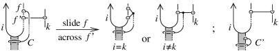
Suppose that is obtained from by passing an edge of some -tree in across a strand of .
![[Uncaptioned image]](/html/2407.15437/assets/x7.png)
-
•
if , then , where is a -tree as shown on the left-hand side of the above figure;444In this figure, parallel bold strands represent any number of parallel strands of the tangle ; we make use of the same convention in all figures of Lemma 2.5.
-
•
if , then (see right-hand side).
-
•
-
(3)
Suppose that is obtained from by passing a leaf of some -tree across a leaf of another -tree (), as illustrated below.
![[Uncaptioned image]](/html/2407.15437/assets/x8.png)
-
•
if left-hand side, then , where is a -tree as shown in the figure;
-
•
if right-hand side, then .
-
•
-
(4)
Let and be two disks obtained by splitting a leaf of some -trees in or , and let and be obtained from by replacing leaf with and , respectively, see figure below. Suppose that is obtained from by replacing with .
![[Uncaptioned image]](/html/2407.15437/assets/x9.png)
-
•
if left-hand side, then ;
-
•
if right-hand side, then .
-
•
-
(5)
Suppose that is obtained from by deleting a pair of -trees or that only differ by a positive half-twist as shown below.
![[Uncaptioned image]](/html/2407.15437/assets/x10.png)
-
•
if left-hand side, then ;
-
•
if right-hand side, then .
-
•
-
(6)
Suppose that and only differ in a neighborhood of a node, in any of the ways represented below. Then .
![[Uncaptioned image]](/html/2407.15437/assets/x11.png)
Sketch of proof.
The proofs are omitted, as they use the same techniques as in [11, §4]; see also [7, 6] and [27, App. E], where similar statements appear. Precise references are as follows. (1) is given in [11, Prop. 4.6]; (2) is proved in [11, Prop. 4.5]; the case of (3) follows from Habiro’s moves 7 and 8, and the case is implicit in [11, pp. 26]; (4) follows from the proof [11, Prop. 4.4]; (5) is a consequence of Habiro’s move 4, see [27, Lem. E.7]; The first two equivalences of (6) follow from the case of (5), and the last equivalence follows from the former two as shown in [27, Lem. E.9]. ∎
We conclude by noting that clasper calculus up to concordance is in practice more flexible. this is in particular illustrated by the following result, see [24, Lem. 4.2].
Lemma 2.6.
Let be a single -tree for the tangle , which contains two simple leaves intersecting the same component as illustrated below. Let be obtained by exchanging the relative positions of these two leaves, as shown in the figure. Then .
2.3. Doubled and parallel -trees
We now introduce two specific types of claspers, that will play central roles in the rest of this paper.
Definition 2.7.
A tree clasper for the tangle is a doubled tree clasper if all its leaves are simple except for one, called doubled leaf, that intersects at exactly two points of the same component. A doubled tree clasper is of parallel type if its doubled leaf intersects at two points with same sign; otherwise, we say that it is of antiparallel type.
Definition 2.8.
A pair of parallel tree claspers for the tangle is a union of two parallel copies of some tree clasper.555We note that there is no ambiguity here in the notion of parallel copies, since for a tree clasper the underlying surface is a disk.
The next two technical results focus on doubled -trees. There are two cases, depending on the type of the doubled tree.
Lemma 2.9.
Let be a doubled -tree of parallel type for a tangle . Then is -concordant to , where is a pair of parallel -trees as shown below.
Proof.
Without loss of generality, we can assume that we are in the situation depicted on the left-hand side of Figure 6.
Applying Lemma 2.5 (4) to split the doubled leaf, we may replace with two simple -trees as shown in the center of the figure, up to -equivalence. Next, we can slide the simple leaf denoted by in the figure, following the orientation of until we obtain the desired pair of parallel -trees. This sliding can be achieved freely up to -concordance, thanks to Lemma 2.5 (1)-(3) and Lemma 2.6. This latter lemma is necessary in the case where another leaf of the -tree containing , is met along the arc along which we are sliding . ∎
Lemma 2.10.
Let be a doubled -tree of antiparallel type for a tangle . The two intersection points of with the doubled leaf then cobound an arc in . Denote also by and the other two leaves of - see the left-hand side of Figure 7. We have the following:
-
(i)
If , then is -equivalent to .
-
(ii)
If and , then is -equivalent to .
-
(iii)
Otherwise, i.e. if only one of and intersects , then is -concordant to .
In particular, we always have that is -concordant to .
Proof.
Figure 7 summarizes the proof of the three cases.
Case (i) is illustrated in the top line. There, the first equivalence is given by Lemma 2.5 (4), while the second equivalence follows from Lemma 2.5 (1)-(3). The result then follows from Lemma 2.5 (5).
The second line gives the proof of case (ii). By Lemma 2.5 (1)-(3) and (6), we obtain the first equivalence.666As the caption of Figure 7 indicates, we actually obtain either the depicted clasper, or the one obtained by inserting a positive half-twist on the -marked edge: the rest of the figure only gives the proof in the untwisted case, the other case being strictly similar. A similar convention is used in the proof of case (iii). The rest of the argument is then exactly the same as in case (i).
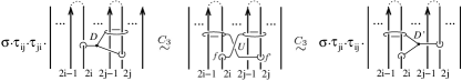
Finally, we prove case (iii), following the third line in Figure 7. We first apply Lemma 2.5 (1)-(3), then (4) and (1)-(3) as in case (ii), to get the first three equivalences. Applying Lemma 2.5 (6) then gives the fourth equivalence. The final step is then given by combining Lemmas 5.1 (1) and 5.2 of [23]. ∎
Corollary 2.11.
As a byproduct of the proof of case (iii), we note the following equivalence.
2.4. The clasper index
We conclude this section with an extra notion associated with claspers, that will be used throughout the rest of this paper.
Let be an -component bottom tangle. Let be a simple -tree for . If intersects the th and th components of as illustrated on the left-hand side of Figure 8 (, possibly ), we say that has index .

Likewise, let be a simple -tree for . If intersects the th, th and th components of as illustrated in the center of Figure 8 (), we say that has index . Note that the index of a -tree is defined only up to cyclic permutations.
This notion extends to doubled -trees, as follows. If the doubled leaf of some doubled tree intersects twice the th component of , then we write instead of when writing the index of . For example, the doubled -tree represented on the the right-hand side of Figure 8 has index .
3. Invariants
This section reviews the definition and relevant properties of the invariants involved in our classification results.
3.1. Invariants for bottom tangles
3.1.1. The Casson knot invariant
The Alexander-Conway polynomial of oriented links is a polynomial in the variable defined by the fact that , where denotes the unknot, and the skein relation
where , and are three links that are identical except in a -ball where they look as depicted.
The Alexander-Conway polynomial of a knot has the form
In particular, the coefficient of in is a knot invariant, called the Casson knot invariant.
Now, we can use the closure-type operations of Figure 3 to define several invariants of bottom tangles, as follows.
Definition 3.1.
Let be an component bottom tangle, and let such that .
-
•
denotes the Casson knot invariant of the closure .
-
•
denotes the Casson knot invariant of the plat closure .
As in the introduction, we simply denote these invariants by and . Note that the latter invariant was first introduced in [21], where it appears under the notation .
3.1.2. Milnor invariants
We now briefly review Milnor invariants of bottom tangles, following [15].777Note that Levine use in [15] the terminology ‘string links’ for what we call here bottom tangles. We also refer the reader to [9] for the equivalent case of string links, and to [18, 19] for the link case originally treated by Milnor.
Let be an -component bottom tangle in . Fix a basepoint in , and denote by the fundamental group of the complement of in . Denote by the canonical meridian elements of represented by the arcs sitting in as shown on the left-hand side of Figure 9.
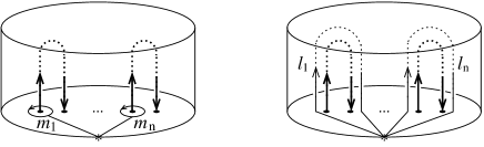
Denote also by the longitude elements, which are represented by parallel copies of each component of as shown on the right-hand side of Figure 9; here we consider preferred longitudes, which are determined by the fact that each is trivial in the abelianization .
As usual in knot theory, a presentation for can be extracted from a diagram of , where each arc of the diagram yields a Wirtinger generator, and each crossing yields a conjugation relation. But the situation turns out to be much simpler when quotienting by the lower central series subgroups.
The lower central series of a group is the descending series of subgroups, defined inductively by and . Let denote the free group on generators . By a theorem of Stallings [32, Thm. 5.1], the map defined by sending to the meridian element for each , induces isomorphisms
for all .
For a fixed level , denote by the image of the th preferred longitude through this isomorphism. The Magnus expansion of is the formal power series in non-commuting variables , obtained by substituting for , and for .
Definition 3.2.
For any sequence of indices in (), the Milnor invariant is the coefficient of in . The length of this Milnor invariant is the length of the sequence .
Length Milnor invariants are set to be zero by convention. Length Milnor invariants () coincide with the linking number of components and , and is therefore sometimes referred to as the triple linking number.
Remark 3.3.
Let be a bottom tangle with vanishing linking numbers. Then it is well known that for length sequences involving only or distinct indices. Indeed if one such invariants were nontrivial, then as first non-vanishing Milnor invariant of it would be equal to the invariant of the closure ; but the latter is necessarily trivial [19, § 4], leading to a contradiction.
3.2. Properties
In this subsection, we gather the main properties of the invariants defined above, that will be used in the proofs of our main results. Let us begin by recalling, in the next two lemmas, some known topological invariance properties.
Recall that link-homotopy is an equivalence relation an tangles, generated by isotopies and self-crossing changes, that is, crossing changes involving two strands of a same component [19]. The following combines results of Stallings [32], Casson [1], and Habegger-Lin [9].
Lemma 3.4.
For any sequence of indices in , Milnor invariant is a concordance invariant. Moreover, if each index in appears at most once in , then is a link-homotopy invariant.
Lemma 3.5.
For any , , , , and are all invariants of -equivalence.
Proof.
It is shown in [11, Thm. 7.2] that all Milnor invariants of length are invariants of -equivalence. The fact that the Casson knot invariant is a -equivalence invariant, is also shown in [11]; this is a consequence of a more general result stating that finite type invariants of degree are -equivalence invariants [11, § 6]. It readily follows that the invariants and also are -equivalence invariants. Finally, the result for is given in [23, Rem. 5.4]. ∎
Using Lemma 3.5, we next show the following variation formulas.
Lemma 3.6.
Let be an -component bottom tangle. Let be indices such that . Let , resp. be a simple -tree of index for , such that there exists a -ball in intersecting , resp. , as shown on the left-hand side, resp. right-hand side, of the figure below.
We have the following variation formulas, for :
-
(i)
, for all ;
-
(ii)
If , , for all such that ;
-
(iii)
, for all such that ;
-
(iv)
, for all such that .
Proof.
We first observe that it suffices to prove these formulas for the case ; the case follows, using Lemma 2.5 (5) and the -invariance Lemma 3.5.
Let us first prove (i). It is clear that if , since becomes trivial when removing the th component of , by Habiro’s move 1. Note that can be regarded as obtained from the trivial bottom tangle by surgery along a union of simple -trees. Hence by Lemma 2.5, the th component of is -equivalent to the connected sum , where is shown on the left-hand side of Figure 5.
Since the Casson knot invariant of the trefoil knot is one, and using the fact that is additive under connected sum and is a -equivalence invariant (Lemma 3.5), the result follows. Formula (ii) follows from the very same arguments, since the image of under the plat-cloture , is a copy of .
We now turn to (iii).
As above, by Habiro’s move 1, the case is clear, so we only consider the case .
For convenience, we give here the proof for the equivalent situation where is an -component string link, which we may regard as obtained from the trivial string link by surgery along a union of tree claspers.
Now, using Lemma 2.5 (1)-(3), we may ’isolate’ up to -equivalence, in the sense that we have . Hence using the -equivalence invariance Lemma 3.5, it suffices to show that .
Observe that is link-homotopic to .888This follows from the main result of [5], but follows also easily from Figure 5. Hence by Lemma 3.4 and Remark 3.3 we have that for any length sequence .
Using the additivity property of Milnor invariants [22, Lem. 3.3], this implies that for any length sequence . The result then directly follows from [23, Lem. 5.3 (3)].
Formula (iv) for Milnor’s triple linking number relies on a similar (though somewhat simpler) argument, using the fact that surgery along is a band sum with a copy of the Borromean rings (Figure 5) whose triple linking number equals .
∎
Remark 3.7.
Building on the proof of (iii), we can further deduce that, if is an index -tree for the trivial string link , then , where denotes the Sato-Levine invariant. Indeed, the th and th components of form a copy of the Whitehead link (Figure 5), which has Sato-Levine invariant .
The following follows directly from Lemma 3.6.
Lemma 3.8.
Let be a pair of parallel -trees for an -component bottom tangle . Then for any , we have , and .
In [20, §3], Miyazawa, Wada and the third author studied the effect of a -move on Milnor invariants. Here, a -move is a local move on tangles that inserts or deletes half-twists on two parallel strands; in particular, a -move is equivalent to a crossing change. The following invariance result shall be useful in Section 4. It is proved using the same techniques as in [20, §3], and is in some sense a weak version of [20, Prop. 3.4].
Lemma 3.9.
Let and be two bottom tangles that differ by a single -move. Then for any sequence of length at most .
Sketch of proof.
The proof follows the very same lines as the proof of [20, Prop. 3.4]. As outlined there, the th longitude of , for any , is essentially obtained from that of by inserting the th power of some elements in the free group on the Wirtinger generators of the fundamental group . The result then follows from the fact that for any word in the free group , we have
(This is an elementary property of the Magnus expansion, which is to be compared with [20, Claim 3.6].) ∎
4. Classifications results for bottom tangles
The purpose of this section is to give classification results for bottom tangles, or equivalently for string links, up to the three equivalence relations involved in our main result. This will in turn be used in the next two sections to tackle the link case.
4.1. Bottom tangles up to clasp-pass moves
As mentioned in Example 2.3, the equivalence relation on tangles generated by clasp-pass moves, is known to be equivalent to the -equivalence defined by Habiro in [11]. The classification of bottom tangles up to -equivalence was given by the first author in [21, Thm. 4.7]:
Theorem 4.1.
Two -component bottom tangles are clasp-pass equivalent if and only if they share all invariants , , and , for any .
4.2. Bottom tangles up to band-pass moves
The equivalence relation generated by band-pass moves, turns out to also be intimately related to Habiro’s notion of -equivalence. More precisely, we have the following, which will be used implicitly throughout the rest of this paper.
Lemma 4.2.
Two tangles are band-pass equivalent if and only if they are -concordant.
Proof.
As mentioned in the introduction, Shibuya showed in [30] that
two concordant tangles are related by self-pass moves.
Hence two -concordant tangles are related by a sequence of self-pass moves and clasp-pass moves. Since these two local moves are realized by a band-pass move, we have the ‘if’ part of the statement.
The ‘only if’ part is shown using clasper calculus. As noted in Example 2.3, two tangles that differ by a band-pass move, are related by surgery along a -tree as shown on the left-hand side of Figure 10.
The first equivalence in the figure follows from Lemma 2.5 (4). Note that the two leaves denoted by and in the figure cobound a sub-arc of the tangle: we can thus slide, say, along this sub-arc until it is adjacent to , and so that the two -trees are parallel as shown on the right-hand side of Figure 10.
There are several obstructions to this sliding: we may have to slide the leaf across some other clasper leaf, and to pass its adjacent edge across some strand of the tangle or some clasper edge. But by Lemma 2.5 (1)-(3), such operation introduce new claspers which are all either of degree or are doubled -trees of antiparallel type. According to Lemma 2.10, all such extra claspers can be removed up to -concordance. Note that we may also have to pass across the other leaf of the doubled -tree containing ; but this is achieved by a mere isotopy, as illustrated in Figure 11.999The figure only shows the proof in the untwisted case; the proof in the case of a positive or negative half-twist is strictly similar.

We deduce the following classification result, which follows from the above lemma, combined with the classification of bottom tangles up to -concordance given by the authors in [23, Thm. 5.8].
Theorem 4.3.
Two -component bottom tangles are band-pass equivalent if and only if they share all invariants , , and , for any .
4.3. Bottom tangles up to band- moves
Recall from the introduction that for any pair of distinct indices , we set . Our third classification result for bottom tangles reads as follows.
Theorem 4.4.
Two -component bottom tangles are band- equivalent if and only if they share all invariants , and , for any .
The rest of this section is devoted to the proof of Theorem 4.4.
4.3.1. Proof of the ‘only if’ part of Theorem 4.4
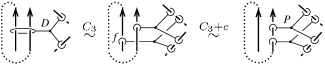
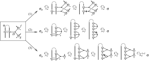
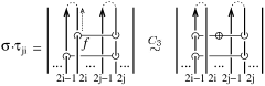
The fact that the mod 4 linking number is invariant under a band- moves is clear from the definition, hence we only need to prove the invariance of and . It is enough to consider the case where is obtained from by a single band- move, which is applied on the th and th components of , possibly with .
Suppose first that . Without loss of generality we can assume that is obtained from by surgery along the -tree illustrated on the left-hand side of Figure 12. We prove below the following :
| (1) |
where is a union of four parallel -trees of index and is a single -tree of index as shown on the right-hand side of Figure 12, and is a union of pairs of parallel -trees.
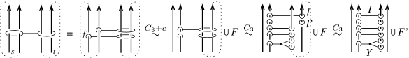
The proof of Equation (1) is illustrated in Figure 12. The first equivalence in the figure follows from Lemma 2.5 (4). The second equivalence is given by Lemma 2.5 (1)-(3) by sliding the leaf labeled along component , following the orientation; this sliding creates extra terms, namely a union of doubled -trees of parallel type, which we may replace with pairs of parallel -trees up to -concordance using Lemma 2.9. The next equivalence in the figure is given by Lemma 2.5 (4), followed by Lemma 2.5 (1)-(3). Finally, we can slide the two leaves labeled by and in the figure along component , following the orientation, until we obtain the union shown on the right-hand side; again, by Lemma 2.5 (1)-(3) this sliding may introduce further pairs of parallel -trees, and Equation (1) follows. We deduce the ‘only if’ part of Theorem 4.4 in the case , as follows (here we pick any ):
- •
- •
- •
The case is for a large part similar. Indeed, we still have the equivalence (1), by a similar argument as the one of Figure 12. The only difference is that the four depicted strands all belong to the same tangle component, and may be met in various orders when running along this component (in other words, we now ignore the dotted parts in the figure). The deformation of Figure 12 can nonetheless be adapted to each of these cases, using Lemmas 2.5 (1)-(3) and 2.9.101010We may also have to use the equivalence illustrated in Figure 11 during the deformation. Hence it suffices to discuss how surgery along , in the case , affects the invariants , and ():
-
•
Surgery along is achieved by self-crossing changes, hence leaves the linking numbers unchanged. On the other hand, this surgery being an -move, we still have by Lemma 3.9 that and are preserved.
-
•
Since is a -tree of index , it follows from [5, Thm. 2.1] that it preserves all Milnor invariant indexed by a sequence such that each index appears at most twice, hence in particular preserves , and .
-
•
As in the case above, Lemma 3.8 ensures that surgery along preserves the invariants and .
This concludes the proof of the ‘only if’ part of Theorem 4.4.
4.3.2. Proof of the ‘if’ part of Theorem 4.4.
Let and be two -component bottom tangles having same invariants , and , for any .
Since a band- move involving components and changes the linking number by , and preserves all other linking numbers, we can construct a bottom tangle which is band- equivalent to , and such that for all indices . Moreover, recall that the (band-) move is an unknotting operation for knots [25, Lem. 3.1]. Hence we may safely assume that for each , the th component of the bottom tangle is isotopic to the th component of . In particular, we thus have that for each . Using the ‘only if’ part of Theorem 4.4, proved in Section 4.3.1, we also have that and for any .
The proof of the following lemma is postponed to the end of this section.
Lemma 4.5.
Let be an -component bottom tangle; let and . There exists a bottom tangle such that
-
•
is band- equivalent to ;
-
•
;
-
•
and share all invariants , , and , for any and .
Using Lemma 4.5, we can construct a bottom tangle , which is band- equivalent to , hence to , and such that and share all invariants , , and , for any .
Theorem 4.3 then implies that and are band-pass equivalent. Since a band-pass move is a composition of band- moves, we have that and are band- equivalent. Hence it only remains to prove the above lemma to complete the proof of Theorem 4.4.
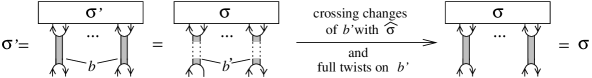
Proof of Lemma 4.5.
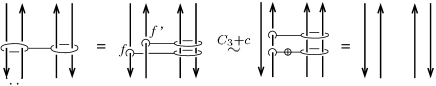
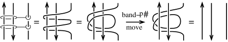
Consider a pair of parallel -trees for the bottom tangle , with index as on the left-hand side of Figure 13. the figure illustrates the fact that and are band- equivalent, as follows. The first equivalence is showed by an isotopy and Lemma 2.5 (4), and the second equivalence is given by Habiro’s move 9. Now, surgery along the -tree shown in the figure, is equivalent to a move, which is a local move defined in Appendix A, which differ from the band-pass and band- moves by the relative orientation of two parallel strands. It is shown in Appendix A, that a move yields band- equivalent tangles. The last equivalence in Figure 13 is then given by clasper surgery and isotopy.
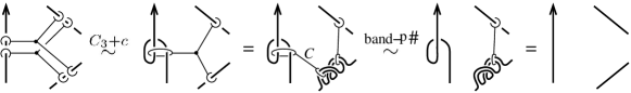
Since the -concordance is generated by band- moves, as follows from Lemma 4.2 and [26, Fig. A.7], we indeed have that and are band- equivalent.
Let us now consider how surgery along affects the invariants of the statement. On the one hand, by Lemma 3.6 (iv) we have that , depending on the orientation of the strands, while all other length Milnor invariants are preserved. On the other hand, and clearly have same linking numbers , since these are -equivalence invariants. The fact that they also share the invariants and , is a direct application of Lemma 3.8. ∎
5. From bottom tangles to links
The purpose of this section is to prove a ‘Markov-type result’, namely Theorem 5.7, which gives necessary and sufficient conditions for two bottom tangles to have clasp-pass, band-pass or band- equivalent closures. We begin by setting up some notation.
For any two indices such that , we define the -component string links , , and as obtained from the trivial string link by surgery along the doubled tree claspers represented in Figure 14. We also define (resp. , and ) as obtained by surgery along the clasper of Figure 14 with a positive half twist inserted on the -marked edge.
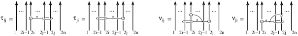
In what follows, we shall also sometimes use the same notation for the clasper given in Figure 14.
Given an -component bottom tangle and a -component string link , let denote the bottom tangle obtained by stacking over as illustrated in Figure 15, equipped with the orientation induced by .

Remark 5.1.
This stacking operation corresponds to Habegger-Lin’s left action of -component string links on -component string links [9], and the ‘Markov-type result’ stated in Theorem 5.7 below for clasp-pass, band-pass and band- equivalence, is in this sense related to [9, Thm. 2.9 and 2.13] for link-homotopy. Specifically, surgery along the -tree corresponds to partial conjugation in [9, Def. 2.12]. A full clasper interpretation of Habegger-Lin’s work, in the context of link-homotopy, is carried out by Graff in [8].
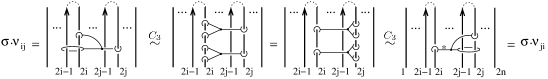
Lemma 5.2.
For any and for any -component bottom tangle , we have .
Proof.
The proof is illustrated in Figure 16. Starting with , applying Corollary 2.11 yields two copies of a simple -tree with index . We then use the symmetry of the Whitehead (string) link (Figure 5), resulting in two copies of a simple -tree with index . Use again Corollary 2.11 then yields .
∎
Lemma 5.3.
Let and be two -component string links in , and let be an -component bottom tangle . Then the bottom tangles and are -equivalent.
Proof.
It suffices to prove the result for , by a case by case verification.
In some cases, the result already holds at the string link level. In the case where (), we have that and are -equivalent by Lemma 2.5 (1)-(3). We also have that in the case and if are pairwise distinct (note that we might need Lemma 2.5 (1)).
We now focus on the case where and for some . Consider the union of doubled -trees for the trivial -component string link represented in the center of Figure 17. On the one hand, sliding upwards the leaf labeled in the figure shows that by Lemma 2.5 (3), where is the doubled -tree shown on the left-hand side of Figure 17. On the other hand, by sliding upwards leaf we likewise obtain that , where is the doubled -tree on the right-hand side. This, together with Lemma 2.10 (i), proves that and are -equivalent for all .
All remaining cases involve and such that exactly of the indices are pairwise distinct. The figure below illustrates the argument for two such cases: applying Lemma 2.5 (1)-(3), we can commute the two -trees at the cost of an additional doubled -tree, and the result follows from Lemma 2.10 (i). All other such cases are treated in a similar way, and are left to the reader.
∎
Definition 5.4.
Let be an -component bottom tangle. Let and be matrices with integer entries, such that the diagonal entries of are 0 and is upper triangular (that is, ). We define the -component bottom tangles and by
where for , and for , denotes the stacking product of copies of .
Remark 5.5.
The bottom tangles and are in general not well-defined from the above formula, since we have not specified any order on the entries of integer matrices. However, in view of Lemma 5.3, their -equivalences classes are well-defined. Since we shall only consider these tangles up to -equivalence in what follows, we may safely use Definition 5.4.
Let us denote by the set of matrices with integer entries whose diagonal entries are all . We denote by
the set of strictly upper triangular integer matrices, and we further set
The proof of the following result is postponed to the end of this section.
Proposition 5.6.
Let and be -component bottom tangles, whose closure and are equivalent. We have the following:
-
(1)
There exists and such that is clasp-pass equivalent to .
-
(2)
There exists a matrix such that is band-pass equivalent to .
-
(3)
There exists a matrix such that is band- equivalent to .
Assuming Proposition 5.6 for now, we obtain the following ‘Markov-type result’ for the three equivalence relations studied in this paper.
Theorem 5.7.
Let and be two -component links, and let and be bottom tangles whose closures and are equivalent to and , respectively. We have the following:
-
(1)
and are clasp-pass equivalent if and only if there exists matrices and such that is clasp-pass equivalent to .
-
(2)
and are band-pass equivalent if and only if there exists a matrix such that is band-pass equivalent to .
-
(3)
and are band- equivalent if and only if there exists a matrix such that is band- equivalent to .
Proof.
We only prove here the first statement: the proof of the other two statements are strictly similar and make use of Proposition 5.6 in the exact same way.
The ‘if’ part of the statement is clear. Indeed, for any and , we have that because
all claspers in Figure 14 become trivial under the closure operation by Habiro’s move 1.
For the ‘only if’ part of the statement, thanks to Lemma 5.3
it is enough to show the case where is obtained from by a single clasp-pass move. Then there exists a bottom tangle which is clasp-pass equivalent to and such that (this is because we can always find ‘closing arcs’ for that are disjoint from a -ball supporting the clasp-pass move.)
By Proposition 5.6 (1), we have that there exists matrices and such that , hence , is clasp-pass equivalent to .
∎
It only remains to prove Proposition 5.6.
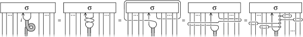
Proof of Proposition 5.6 (1).
We regard the bottom tangle as a band sum of and the trivial bottom tangle, along a union of ‘trivially embedded’ bands as illustrated on the left-hand side of Figure 18.
Performing an isotopy turning into , and further isotopies of the attaching regions of the bands, we obtain a decomposition of as a band sum of and the trivial bottom tangle. This band sum is along the image of under these isotopies; these bands are thus knotted and linked together and with . Therefore can obtained from this band sum by crossing changes between the bands and strands of , and adding full-twists to , see Figure 18. Note that a crossing change between bands of can be realized by the former deformations. By Lemma 5.3, it is enough to consider each of these deformations of the bands independently.
We note that adding a full twist to the th band, is achieved by surgery along a union of doubled -trees , see Figure 19.111111The figure only illustrates the case of a negative full twist, but the positive case is similar.
Now, a crossing change between the th component of and the th component of (possibly ), is achieved by surgery along a doubled -tree whose doubled leaf intersects transversely (see the left-hand sides of Figures 20 and 21).
We may regard as obtained from the trivial link by surgery along a union of simple -trees (Example 2.3).
Let us distinguish two cases.
The case where is summarized in Figure 20.
We aim at dragging the simple leaf of towards the band , so as to obtain a copy of or (see the right-hand side of the figure).
This is achieved by passing successively the leaf through some leaves of , and passing the edge of across some tangle strand: by Lemma 2.5 (1)-(3), each such operation can be achieved, up to -equivalence, at the cost of an additional doubled -trees, and we only have to show that up to -equivalence, all such extra terms are either copies of or can be deleted. As Figure 20 illustrates,121212The figure shows the case of a leaf exchange, but the operation passing the edge of across a tangle strand is treated similarly. there are two subcases:
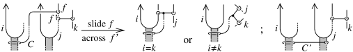
The case where is illustrated in Figure 21. Dragging the simple leaf of yields the doubled -tree shown on the right-hand side, and is equivalent to a union of (see the left-hand side of Figure 11 and Figure 19). As in the previous case, we analyse the additional doubled -trees that may appear in this dragging process:
-
•
if , then the extra term given by a leaf exchange is a doubled -tree with index as shown in the figure, and by Lemma 2.10 (ii) it can be deleted up to -equivalence;
-
•
if , the leaf exchange introduces a copy of up to -equivalence, and we conclude as in the preceding case.
Hence we have shown that can be deformed into at the cost of stacking copies of () and (), and the proof is complete. ∎
Proof of Proposition 5.6 (2).
6. Proof of Theorems A and B
In this section we prove our main results. The clasp-pass classification of links, Theorem 1, follows directly from the combination of Theorem 4.1, Theorem 5.7 (1) and Proposition 6.1 below. The classification of links up to band-pass and band- moves, Theorem 2, is obtained in the same way from Theorems 4.3, 4.4 and Proposition 6.1 (1),(3).
Proposition 6.1.
Let be an -component bottom tangle. Let and . For any , we have the following:
-
(1)
and .
-
(2)
and .
-
(3)
and
Proof.
Part (1) of the statement is clear. On one hand, all four claspers depicted in Figure 14 become trivial when taking the closure of the th component of and deleting all other components, so that the resulting knot is isotopic to the closure of the th component of , hence has same invariant . On the other hand, it is readily checked that surgery along all four claspers depicted in Figure 14 preserves the linking numbers.
Part (2) addresses the variation of and under stacking over the string link , that is, under surgery along the doubled -trees (). Since is link-homotopic to , we immediately have that by Lemma 3.4. Moreover, using Corollary 2.11, the fact that follows directly from Lemma 3.6 (ii).
It thus remains to prove part (3), which investigates the effect of surgery along the -trees and (). Recall from [26, 17] that the -equivalence of (string) links, which is known to coincide with the -equivalence (Example 2.3), is classified by the linking numbers. Hence by Lemma 2.5 we have
where
-
•
is an -component bottom tangle obtained from the trivial one by surgery along -trees;
-
•
, where is the -component string link represented on the left-hand side of Figure 23, and where the product is taken using the lexicographic order.
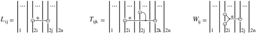
Figure 24 illustrates the effect of stacking over .
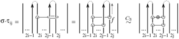
The first equivalence is given by Lemma 2.5 (4). The idea is then to slide the leaf marked against the orientation of , until we obtain two parallel -trees that differ by a twist as shown in the figure: Lemma 2.5 (5) then ensures that these two -trees cancel. Sliding in this way, involves passing it across all leaves in intersecting the th component; using Lemma 2.5 (1)-(3) repeatedly, this yields the equivalence
where , resp. , is the -component string link represented on the middle, resp. right-hand side, of Figure 23. The following formulas then directly follow from Lemma 3.6.
| (2) |
Figure 25 likewise illustrates the effect of stacking over .
Appendix A Links and bottom tangles up to moves
A.1. The - and -moves
A natural variant of the pass- and -moves, is the -move illustrated in the center of Figure 26.
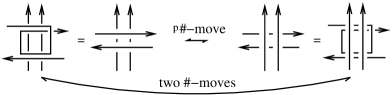
The figure shows how, using the same argument as Murakami and Nakanishi in [26, Fig. A.7], a -move can be realized by two applications of the -move. The same trick shows that a pass-move is achieved by two -moves. In fact, we have the following simple fact.
Proposition A.1.
The equivalence relation generated by the -move, coincides with the pass-equivalence.
Proof.
This readily follows from the above observation and the figure below, which illustrates the fact that a -moves can be realized by two pass-moves.
∎
A move is naturally defined as a -move such that each pair of parallel strands are from the same components.
The observation in Figure 26 shows that the move defines an intermediate equivalence relation between the band-pass and the band- equivalence. However, the proof of Proposition A.1 no longer applies to the case of a move. As a matter of fact, the classification results stated below show that the equivalence is different from the band-pass equivalence or the band- equivalence.
Remark A.2.
A.2. Classification results
This section briefly outlines how the techniques and results of this paper can be simply adapted to the equivalence.
The key observation is that surgery along a pair of parallel -trees yields equivalent tangles. This is apparent from Figure 13, which summarizes the proof of Lemma 4.5. In particular, this means that the technical Lemma 4.5 still holds, when replacing the band- equivalence with the equivalence.
Since the move is achieved by two band- moves (Figure 26), it preserves . It also preserves since is a band- equivalence invariant (Theorem 4.4), and is a -equivalence invariant. Using the above-mentioned refined version of Lemma 4.5 for equivalence, the proof of the ‘if’ part of Theorem 4.4 can be adapted. Hence we have the following.
Theorem A.3.
Two -component bottom tangles are -equivalent if and only if they share all invariants , , and , for any .
Since is equivalent to the trivial string link (see Figure 22), Proposition 5.6 (3) and Theorem 5.7 (3) still hold for the equivalence. Hence the proof of Theorem 2 (2) can be straightforwardly adapted to establish the following classification theorem.
Theorem A.4.
Let and be -component links, and let and be bottom tangles whose closures and are equivalent to and respectively. The links and are -equivalent if and only if and share all invariants and and the following system has a solution over .
The classification of bottom tangles up to -equivalence can be likewise obtained in a straightforward way.
References
- [1] A. J. Casson, Link cobordism and Milnor’s invariant, Bull. London Math. Soc. 7 (1975), 39–40.
- [2] L. Cervantes and R. A. Fenn, Boundary links are homotopy trivial, Quart. J. Math. Oxford Ser. (2), 39 (1988), 151–158.
- [3] J. Conant, R. Schneiderman and P. Teichner, Whitney tower concordance of classical links, Geom. Topol., 16 (2012), 1419–1479.
- [4] J. Conant, R. Schneiderman and P. Teichner, Clasper concordance, Whitney towers and repeating Milnor invariants, preprint (2020), arXiv:2005.05381.
- [5] T. Fleming and A. Yasuhara, Milnor’s invariants and self -equivalence, Proc. Amer. Math. Soc. 137 (2009) 761–770.
- [6] S. Garoufalidis, M. Goussarov and M. Polyak, Calculus of clovers and finite type invariants of 3-manifolds, Geom. Topol. 5 (2001) 75–108 (electronic).
- [7] M. Goussarov, Variations of knotted graphs. The geometric technique of -equivalence, Algebra i Analiz 12 (2000) 79–125.
- [8] E. Graff, On braids and links up to link homotopy, to appear in J. Math. Soc. Japan.
- [9] N. Habegger and X.S. Lin, The classification of links up to link-homotopy, J. Amer. Math. Soc. 3 (1990), 389–419.
- [10] K. Habiro, Clasp-pass moves on knots, unpublished (1993).
- [11] K. Habiro, Claspers and finite type invariants of links, Geom. Topol. 4 (2000), 1–83.
- [12] K. Habiro, Bottom tangles and universal invariants, Algebr. Geom. Topol., 6 (2006), 1113–1214.
- [13] L.H. Kauffman, Link manifolds, Michigan Math. J., 21 (1974), 33–44.
- [14] L.H. Kauffman, Formal Knot Thoery, Math. Notes No. 30, Princeton Univ. Press, 1983.
- [15] J. P. Levine, The -invariants of based links, Differential topology (Siegen, 1987), 87–103, Lecture Notes in Math. 1350, Springer, Berlin, (1988).
- [16] T.E. Martin, Classification of links up to 0-solvability, Topology Appl., 317 (2022), Paper No. 108158.
- [17] S.V. Matveev, Generalized surgeries of three-dimensional manifolds and representations of homology spheres, Mat. Zametki, 42 (1987), 268–278, 345 (in Russian): English transl. in: Math. Notes 42, 651–656 (1987)
- [18] J. Milnor, Link groups, Ann. of Math. (2) 59 (1954), 177—195.
- [19] J. Milnor, Isotopy of links, Algebraic geometry and topology, A symposium in honor of S. Lefschetz, Princeton University Press, Princeton, N. J., (1957), 280–306.
- [20] H.A. Miyazawa, K. Wada and A. Yasuhara, Classification of string links up to -moves and link-homotopy, Ann. Inst. Fourier (Grenoble), 71 (2021), 889–911.
- [21] J.B. Meilhan, On Vassiliev invariants of order two for string links, J. Knot Theory Ramifications, 14 (2005) 665–687.
- [22] J.B. Meilhan and A. Yasuhara, On -moves for links, Pacific J. Math. 238 (2008) 119–143.
- [23] J.B. Meilhan and A. Yasuhara, Characterization of finite type string link invariants of degree , Math. Proc. Cambridge Philos. Soc. 148 (2010) 439–472.
- [24] J.B. Meilhan and A. Yasuhara, Abelian quotients of the string link monoid, Alg. Geom. Topol. 14 (2014) 1461–1488.
- [25] H. Murakami, Some metrics on classical knots, Math. Ann., 270 (1985) 35–45.
- [26] H. Murakami and Y. Nakanishi, On a certain move generating link-homology, Math. Ann. 284 (1989) 75–89.
- [27] T. Ohtsuki, Quantum invariants, Series on Knots and Everything 29, World Scientific Ed., River Edge, NJ, 2002.
- [28] M. Saito, On the unoriented Sato-Levine invariant, J. Knot Theory Ramifications, 2, (1993) 335–358.
- [29] T. Shibuya, Self -unknotting operation of links, Mem. Osaka Inst. Tech. Ser. A, 34 (1989), 9–17.
- [30] T. Shibuya, Self--equivalences of homology boundary links, Kobe J. Math., 9, (1992) 159–162.
- [31] T. Shibuya and A. Yasuhara, Classification of links up to self pass-move, J. Math. Soc. Japan, 55, (2003) 939–946.
- [32] J. Stallings, Homology and central series of groups, J. Algebra (1965), 170–181.
- [33] K. Taniyama and A. Yasuhara, Clasp-pass moves on knots, links and spatial graphs, Topology Appl. 122, (2002) 501–529.
- [34] T. Tsukamoto, Clasp-pass move and Vassiliev invariants of type three for knots, Proc. Amer. Math. Soc., 128 (2000), 1859–1867.