Spatial-Division Augmented Occupancy Field for Bone Shape Reconstruction from Bi-Planar X-Rays – Supplementary Material

Figure 5: More quantitative comparison results evaluated at $128^{3}$ output resolution.

1 Implementation Details

Voxel-based Methods. We implement the 5 voxel-based representation using the code implementation in  [shakya2024benchmarking]. They have already configured proper parameters for each method via hyperparameter search, including the structure (channel, depth) settings, learning rate, batch size, and optimizer.

Implicit-representation-based Methods. We implement SdAOF using PyTorch with a single NVIDIA RTX 3090 GPU. Here we introduce key implementation details. Please refer to supplementary material for more configurations. We use UNet as the feature extractor with output feature channel $C=128$. The output features of each double convolution layer, excluding the input convolution, contribute to distillation, resulting in $L=9$ layers utilized for this purpose. The subspace division number is set to $K=4$. During each forward pass, $N=10000$ points are sampled. Half of these points are uniformly distributed across the space, while the remainder is sampled from a region within 2mm of the surfaces. Given that each occupancy field can represent only one watertight bone surface, we set the output channel to 2 for deriving the left and right pelvic surfaces. The loss balance term $\alpha$ in Eqn. (LABEL:overall_loss) is empirically set to 0.2. Both PIFu and SdAOF use the same set of hyperparameters. Specifically, we use the Adam optimizer with an initial learning rate of 5e-3. The learning rate is linearly warmed up from 5e-5 to 5e-3 during the first 25 epochs, then decays by multiplying a factor of 0.8 after at $\{50,100\}$ epoch. Both PiFU, teacher OF Network, and SdAOF are trained for 110 epochs. The MLP for occupancy value prediction consists of 6 layers with skip connection (channels: $512\rightarrow 1024\rightarrow 512\rightarrow 256\rightarrow 128\rightarrow 2$).

2 Evaluation Metrics

The Chamfer Distance (CD) and Earth Mover’s Distance (EMD) measures dissimilarity between two point sets. In mesh reconstruction context, $N$ points are uniformly sampled from the predicted mesh surface and ground-truth mesh surface for calculation, denoted by $S_{\text{pred}},S_{\text{GT}}\subseteq\mathbb{R}^{3}$. In practice, we set $N=4096$.

Chamfer Distance. CD measures both the reconstruction accuracy and completeness by calculating the average distance from each point in one set to its nearest neighbor in another set and vice versa. It is defined as

$$\text{ CD }(S_{\text{pred }},S_{\text{GT}})=\frac{1}{2}(\frac{1}{\left|S_{\text{pred }}\right|}\sum_{p\in S_{\text{pred}}}\min_{q\in S_{\text{GT}}}\|p-q\|_{2}+\frac{1}{\left|S_{\text{GT }}\right|}\sum_{q\in S_{\text{GT}}}\min_{p\in S_{\text{pred}}}\|p-q\|_{2}).$$ (7)

Earth Mover’s Distance. Earth Mover’s Distance (EMD) measures a better perceptual similarity assessment compared to other distance measures. Given two sets, one can be seen as a mass of earth properly spread in space, the other as a collection of holes in that same space. EMD calculates the minimum work required to fill the holes with earth. The work unit corresponds to a unit of Euclidean distance. Its calculation is formulated by

$$\text{EMD}(S_{\text{pred}},S_{\text{GT}})=\frac{1}{\left|S_{\text{pred}}\right|}\min_{\phi:S_{\text{pred}}\rightarrow S_{\text{GT}}}\sum_{p\in S_{\text{pred}}}\|p-\phi(p)\|_{2},$$ (8)

where $\phi:S_{\text{pred}}\rightarrow S_{\text{GT}}$ is a bijection.

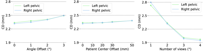
Figure 6: Additional experiment results evaluate at $336^{3}$ output resolution.

3 Additional experiments

Robustness to different imaging parameters. In real-world scenarios, the imaging direction may deviate from the perfect alignment with AP and lateral views, and the patient’s center may vary. These deviations cause the magnification effect within X-ray images to differ from the training distributions, which assume ideal bi-planar view directions and iso-center patients. The results presented in Fig. 6 demonstrate that SdAOF exhibits robustness to minor variations in both view angles and patient center locations.

Extension to multi-view input. The proposed SdAOF can naturally extend to multiple view directions. The right part of Fig. 6 illustrates the CD of SdAOF when using 1 to 4 input views (with the AP view as the single input view). These results highlight that SdAOF consistently enhances the reconstruction quality with an increasing number of input views. This flexibility provides a trade-off between radiation dose and improved accuracy in various application scenarios.